Large Intelligent Surfaces with Low-End Receivers: From Scaling to Antenna and Panel Selection

Abstract

We analyze the performance of large intelligent surface (LIS) with hardware distortion at its RX-chains. In particular, we consider the memory-less polynomial model for non-ideal hardware and derive analytical expressions for the signal to noise plus distortion ratio after applying maximum ratio combining (MRC) at the LIS. We also study the effect of back-off and automatic gain control on the RX-chains. The derived expressions enable us to evaluate the scalability of LIS when hardware impairments are present. We also study the cost of assuming ideal hardware by analyzing the minimum scaling required to achieve the same performance with a non-ideal hardware. Then, we exploit the analytical expressions to propose optimized antenna selection schemes for LIS and we show that such schemes can improve the performance significantly. In particular, the antenna selection schemes allow the LIS to have lower number of non-ideal RX-chains for signal reception while maintaining a good performance. We also consider a more practical case where the LIS is deployed as a grid of multi-antenna panels, and we propose panel selection schemes to optimize the complexity-performance trade-offs and improve the system overall efficiency.

I Introduction

Large Intelligent Surfaces (LISs) have emerged as one of the next major steps in the future development of multiple-input multiple-output (MIMO) communication systems [1, 2, 3]. While LISs are sometimes considered to be a scaled up version of the widely known massive MIMO systems, they have some unique properties which distinguishes them from the massive MIMO systems. For instance, their physical size can be compared to the user-equipment (UE) distance to the LIS, which introduces near-field effects in the wireless channel. As a result, the common assumptions about the massive MIMO channels are no longer valid and new effects emerge. This requires different channel models, and more investigation into the already known facts about the transmit and receive schemes in massive MIMO systems [4]. More importantly, the deployment of LISs is envisioned to be much more challenging because of the enormous leap in the number of transceiver chains, and the associated processing complexities. One important challenge is the cost efficiency of the whole system, where hundreds to thousands of transceiver chains are to be deployed, which may force systems designers to consider the use of inexpensive hardware components in each of these transceiver chains [5]. Therefore, it is of high importance to study and mitigate the effects of hardware distortion in transceiver chains when scaling up LIS to allow the use of cost-efficient transceiver chains.

The vision for future antenna arrays in the next generation of wireless communication systems highly depends on deploying arbitrarily large arrays due to the compelling gains in terms of multiplexing and beamforming performance through increasing spatial resolution [6]. With traditional design approaches, implementing such a huge array may not be economically favored for operators and vendors, since each antenna is typically equipped with an analog and a digital front-end (AFE and DFE) [7]. The requirements for each transceiver chain may lead to unreasonable implementation costs [8]. On the other hand, the power consumption of each transceiver can also become a bottleneck, especially if there are tight requirements on the non-linearity of amplifiers and the out-of-band emissions. AFEs are considered to be one of the main sources of hardware distortion in receivers [9, 10, 11]. Not only the non-linearity effect of AFEs are important to consider, but also the limitations in the total power consumption of the receiver chain is of great importance. Linearity requirements in the RX-chains can result in a huge leap in power consumption of the whole system [12], which is not favorable neither in terms of cost nor energy efficiency.

To deal with these challenges, we need to make the receiver design as efficient as possible, from a system perspective. In general, the path to follow is to optimize the signal processing schemes and system designs while maintaining the hardware quality at a minimum level. In other words, we want to get the most gain from each transceiver chain while limiting the implementation costs, e.g., by using inexpensive hardware components. In [13] and [14], we have proposed approaches to address such challenges in massive MIMO systems, mainly by optimizing the per-antenna digital pre-distortion (DPD) resources. Another approach is to perform antenna selection methods and only use a portion of the array for transmission and reception. By doing so, we only use antennas which have a significant contribution to the performance and thereby increase energy efficiency.

In this paper, we focus on optimizing the performance of LIS with non-ideal RX-chains. We first analyze the signal to distortion-plus-noise ratio (SNDR) with the purpose of studying the scaling behavior and asymptotic limits of LIS with hardware distortion. Then, we propose receive antenna selection schemes for a LIS with non-ideal AFEs. Optimization problems are defined and solved to illustrate the importance of performing antenna selection when scaling up LIS. We show that selecting antennas with the strongest channels is not always the optimal solution. We then focus on more practical cases where the LIS is implemented as a grid of panels, and transform the antenna selection problem into a panel selection problem. Low-complexity closed-form sub-optimal solutions are proposed for the panel selection. We also show that, by adopting such antenna selection and panel selection schemes, we can improve the system performance significantly for a fixed receive-chain hardware quality.

I-A Contributions

The contributions of this paper are listed as follows.

• We provide a framework to study the hardware distortion effect on LIS performance while considering high-complexity non-linear polynomial model at RX-chains.

• We derive close-form expressions for the SNDR of the LIS under polynomial hardware distortion model to enable scaling and asymptotic analysis.

• We introduce antenna selection problems in LIS with hardware distortion and illustrate the achievable gains of adopting optimal antenna selection. We also consider the the more practical case with a panel-based LIS and propose closed-form solutions for panel selection with hardware distortion effects.

I-B Paper Outline

The rest of this paper is organized as follows. In Section II, the system model is introduced, which includes the LIS deployment configurations, channel model, and hardware distortion model. In Section III, we characterize the SNDR and propose closed-form expressions to evaluate the LIS performance, which is exploited for asymptotic and scaling analysis. Sections IV and V introduce the antenna and panel selection problems, respectively, and some proposed solutions are presented for the corresponding LIS scenarios. In Section VI, numerical results are used to further illustrate the results from previous sections. Finally, Section VII concludes the paper results.

I-C Notation

Matrices, vectors, and scalars are denoted by boldface uppercase, boldface lowercase, and italic letters, respectively. For a vector $\bm{a}$, conjugate transpose, transpose, Euclidean norm, and the $i$’th element of $\bm{a}$ are represented by $\bm{a}^{H}$, $\bm{a}^{T}$, $\|\tilde{\bm{a}}\|$, and $a_{i}$, respectively. For a scalar $a$, the complex conjugate is denoted by $\bar{a}$. We indicate zero-mean circularly-symmetric complex Gaussian random vectors with covariance matrix $\bm{C}$ as $\bm{a}\sim\mathcal{CN}(\bm{0},\bm{C})$ and the expectation of a random variable by $\mathbb{E}\{\cdot\}$. We denote a diagonal matrix with elements ${a_{1},...,a_{N}}$ on the main diagonal by $\textnormal{diag}\left({a_{1},...,a_{N}}\right)$ and the $N\times N$ identity matrix by $\bm{I}_{N}$.

II System Model

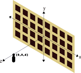
Figure 1: Array and UE configuration with coordinate system.

We consider an uplink scenario where a LIS consisting of $N\gg 1$ antenna elements serves a single-antenna user equipment (UE), which transmits the complex base-band symbol $s\in\mathbb{C}$ with $\mathbb{E}\{|s|^{2}\}=P$, over a narrow-band channel $\bm{h}\in\mathbb{C}^{N\times 1}$. Each receive antenna is equipped with a non-ideal RX-chain, introducing distortion into the received signal. The received signal after going through the RX-chains is expressed as

$$\bm{r}=f\left(\bm{h}s\right)+\bm{n},$$ (1)

where $f(\cdot):\mathcal{C}^{N\times 1}\rightarrow\mathcal{C}^{N\times 1}$ models the overall non-ideal effects at the receiver AFEs and DFEs of the LIS, and $\bm{n}\sim\mathcal{CN}(\bm{0},\sigma^{2}\bm{I}_{N})$ is the additive noise.

The LIS is assumed to be spanned on the $x$-$y$ plane with its center located at the origin. Fig. 1 illustrates the configuration of the LIS and the UE. In [1], the following channel model is adopted, which we use in the analytical part of this paper. For analytical tractability, we assume a narrow-band LOS scenario where the channel $h(x,y)=|h(x,y)|~{}\text{exp}\left(-j\phi(x,y)\right)$ between the UE in Fig. 1 and a point on the LIS with coordinates $(x,y,0)$ has the squared amplitude given by

$$|h(x,y)|^{2}=\frac{1}{4\pi(d^{2}+x^{2}+y^{2})}\frac{d}{\sqrt{d^{2}+x^{2}+y^{2}}},$$ (2)

and the phase based on propagation delay as

$$\phi(x,y)=2\pi\frac{\sqrt{d^{2}+x^{2}+y^{2}}}{\lambda},$$ (3)

where $\lambda$ is the wavelength. For the $n$’th antenna element, located at $(x_{n},y_{n},0)$ with effective area $A$ small enough such that $|h(x,y)|^{2}$ is almost fixed inside its effective area, the channel gain is $|h_{n}|^{2}=A|h(x_{n},y_{n})|^{2}$.

While this form of deployment is a common vision for the LIS implementation in the future of wireless networks [15], it is not favorable with current technology from a practical point of view [16]. A potentially more favorable option, without losing practicality and cost efficiency is to implement the LIS as grid of panels, each equipped with some equally distanced antenna elements [7]. Fig. 2 illustrates an example of panel configuration of a LIS on the $x$-$y$ plane.

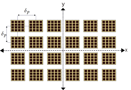
Figure 2: Panels configuration with coordinate system, with a fixed distance $\delta_{p}$ between adjacent panels.

II-A Hardware distortion model

There are several models to opt for the distortion function $f(\cdot)$ in (1) and the model selection is always a trade-off between accuracy and analytical tractability. One of the common models in the literature is the memory-less polynomial, which has an high accuracy in most cases, at the cost of high complexity in the analytical results. We mainly focus on this model throughout this paper to guarantee the accuracy of the analysis. In this model, the input-output relation of an RX-chain for a complex input $x\in\mathbb{C}$ is given by

$$y=f(x)=\sum_{k=0}^{L-1}a_{2k+1}~{}x|x|^{2k},$$ (4)

where $a_{2k+1}\in\mathbb{C}$ are the model parameters, typically estimated based on input-output measurements on the RX-chains. This model only considers odd orders since they are the main source of in-band distortion. For an ideal RX-chain, we have $L=1$ and $a_{1}=1$.

Let us first analyze the distortion behaviour for a single RX-chain. To isolate the distortion from the desired signal, we can rewrite (4) by using the linear minimum mean squared error (LMMSE) of $y$ given $x$ as

$$y=\frac{C_{yx}}{C_{xx}}x+\eta,$$ (5)

where $C_{yx}$ is the covariance between $y$ and $x$, $C_{xx}$ is the auto-correlation of $x$, and $\eta$ is the estimation error. Equation (5) also corresponds to the Bussgang decomposition, which is a popular tool in hardware distortion analysis [17]. By defining $g={C_{yx}}/{C_{xx}}$ as the Bussgang gain and noting that $\eta$ is uncorrelated with $x$, the auto-correlation of $\eta$ is given by

$$C_{\eta\eta}=C_{yy}-|g|^{2}C_{xx},$$ (6)

which can be calculated using the following lemma.

Lemma II.1

Given the memory-less polynomial model in (4), together with its Bussgang equivalent form, and assuming a Gaussian input distribution, i.e. $x\sim\mathcal{CN}(0,P)$, we can calculate the Bussgang gain as

$$g=\frac{\mathbb{E}\left[y\bar{x}\right]}{\mathbb{E}\left[|x|^{2}\right]}=\sum_{k=0}^{L-1}a_{2k+1}(k+1)!P^{k},$$ (7)

and the distortion power as

$$C_{\eta\eta}=\mathbb{E}\left[|\eta|^{2}\right]=\sum_{k=1}^{2L-1}\left(k!P^{k}\sum_{i=1}^{k}a_{2i-1}\bar{a}_{2k-2i+1}\right)-|g|^{2}P,$$ (8)

where $P=\mathbb{E}\left[|x|^{2}\right]$.

Proof:

See Appendix A. ∎

In many cases, the 3rd order non-linearity term, $a_{3}$, is the dominant source of RF-hardware distortions [18, 19]. For the special case of 3rd order non-linearity, i.e. $L=2$, Lemma (II.1) gives

$$g=a_{1}+2a_{3}P,$$ (9)

and

$$C_{\eta\eta}=2|a_{3}|^{2}P^{3},$$ (10)

which we will use in Section V for panel selection.

II-B Automatic gain control (AGC) and back-off

As mentioned earlier, the model coefficients are estimated based on input-output measurements of the RX-chain. The results are usually reported for a normalized input with unit maximum amplitude [20]. Given the estimated parameters $\hat{a}_{2k+1}$, for the normalized input, if the actual input to the receiver has an amplitude range of $0<|{x}|<V_{max}$, we can use the following conversion to adapt the normalization

$$a_{2k+1}=\frac{\hat{a}_{2k+1}}{(V_{\text{max}}^{2})^{k}}.$$ (11)

The value of $V_{\text{max}}$ can be controlled in the receiver by applying back-off to its input, either by using alternators or by performing gain control schemes in the RX-chain amplifiers. The back-off is applied to prevent clipping, which may cause severe hardware distortion at the receivers. In our system, we define $V_{\text{max}}^{2}=b_{\text{off}}P_{\text{max}}$, where $b_{\text{off}}$ is the fixed back-off factor and $P_{\text{max}}$ depends on the gain control scheme at the receiver. In a typical LIS scenario, the received power at each antenna element can have a high dynamic range, which makes the interplay between the back-off, gain control, and hardware distortion of great importance.

The back-off value, $b_{\text{off}}$, is a design parameter which can be selected based on the dynamic range of the received power across the LIS. The gain control term, $P_{\text{max}}$, on the other hand can be set either to a fixed value for all the antenna elements, or depending on the received power on each antenna, which may be achieved by introducing per-antenna automatic gain control (AGC) in the amplifiers. The latter case may be of less interest from a practical point of view in LIS scenarios since there are hundreds to thousands of RX-chains across the LIS, with a high variation of the received power. Therefore, having a perfect gain control unit on each antenna element can contribute to the already high complexity of the whole system, apart from increasing implementation costs. On the other hand, applying a fixed gain control is simpler and less expensive to implement, but has the disadvantage of excessive gain reduction on some antennas, which can reduce the energy efficiency of the amplifiers. In this paper we study both cases and compare their performance.

If all RX-chains are capable of performing individual AGC, the per-antenna coefficients $a_{k,n}$ become

$$a_{2k+1,n}=\frac{\hat{a}_{2k+1}}{(b_{\text{off}}P\left|{h}_{n}\right|^{2})^{k}},$$ (12)

and, in this case, calculating the Bussgang parameters in Lemma II.1 results in a fixed Bussgang gain

$$\tilde{g}=\sum_{k=0}^{L-1}\frac{\hat{a}_{2k+1}}{b_{\text{off}}^{k}}(k+1)!$$ (13)

for all antenna elements. The distortion power, on the other hand, is a linearly increasing function of the input power to the corresponding antenna, i.e. $C_{n}=\kappa\left|{h}_{n}\right|^{2}P$, where

$$\kappa=\sum_{k=1}^{2L-1}\left(\frac{k!}{b_{\text{off}}^{k-1}}~{}\sum_{i=1}^{k}\hat{a}_{2i-1}\bar{\hat{a}}_{2k-2i+1}\right)-\left|\tilde{g}\right|^{2}.$$ (14)

We may thus note that by assuming per-antenna perfect AGC, the Bussgang gain and the distortion growth rate are independent of the input power or the antenna index across the LIS.

As we will see in the next section, the assumption of per-antenna AGC can reduce the complexity of the analysis. Interestingly, the linear growth rate in (14) can be seen as a bridge from the memory-less polynomial model in (4) to the conventional additive linear distortion model, which is widely used in literature [21]. One should note that the additive linear distortion model is a rough and simple approach of modeling the hardware distortion, where the single parameter $\kappa$ denotes the severeness of the hardware distortion and can be interpreted as a measure of RX-chain hardware quality. In general, perfect per-antenna AGC assumption and the additive linear model are not accurate. Such assumptions imply that, no matter what the input power is, the Bussgang gain, $\tilde{g}$, and the distortion growth rate, $\kappa$, are constants. Nevertheless, we consider both the case where per-antenna AGC is employed, as well as the case with fixed gain control, for completeness and to gain better understanding of the impact of such assumptions.

III SNDR Characterization

By using the same technique as in (5) which is based on LMMSE or Bussgang decomposition, the received signal in (1) may be expressed as

$$\bm{r}=\bm{G}\bm{h}s+\bm{\eta}+\bm{n},$$ (15)

where $\bm{G}=\text{diag}\left(g_{1},\dots,g_{N}\right)$, $\bm{C_{\eta\eta}}=\text{diag}\left(C_{1},\dots,C_{N}\right)$, with $g_{n}$ and $C_{n}$ corresponding to the Busssgang gain and distortion power for the $n$’th antenna as given in (7) and (8), respectively. For analytical tractability and based on the results from [22], we have assumed that the distortion correlation among the antennas are negligible, i.e. $\bm{C_{\eta\eta}}$ is diagonal.

The LIS applies a combing vector $\bm{v}$ to the received signal $\bm{r}$ to equalize the transmitted signal. Maximum Ratio Combining (MRC) is an attractive option in LIS scenarios because of its simplicity and reasonable performance, since it still allows us to exploit the available spatial degrees of freedom[1]. In our scenario, the MRC vector may be expressed as $\bm{v}^{T}=\tilde{\bm{h}}^{H}/\|\tilde{\bm{h}}\|$ where $\tilde{\bm{h}}=\bm{G}\bm{h}$, can be interpreted as the effective channel, which includes the physical channel and the multiplicative hardware distortion effect. In fact, the LIS would only be able to estimate the effective channel $\tilde{\bm{h}}$ from the uplink UE pilots since the signals received during channel estimation are also affected by the hardware distortion. We assume that the LIS has a perfect estimate of $\tilde{\bm{h}}$ so that we can isolate the effect of hardware distortion from that of channel estimation imperfections. Note that the estimation error would only correspond to an uncorrelated additive term, which would effectively not affect our analysis on hardware distortion.

By applying the combining vector $\bm{v}^{T}=\tilde{\bm{h}}^{H}/\|\tilde{\bm{h}}\|$ to $\bm{r}$, we reach

$$\bm{v}^{T}\bm{r}=\left(\tilde{\bm{h}}^{H}\tilde{\bm{h}}s+\tilde{\bm{h}}^{H}\bm{\eta}+\tilde{\bm{h}}^{H}\bm{n}\right)/\|\tilde{\bm{h}}\|,$$ (16)

and the corresponding SNDR can be calculated as

$$\gamma=\frac{P\sum_{n=1}^{N}\left|\tilde{h}_{n}\right|^{2}}{\frac{\sum_{n=1}^{N}C_{n}\left|\tilde{h}_{n}\right|^{2}}{\sum_{n=1}^{N}\left|\tilde{h}_{n}\right|^{2}}+\sigma^{2}},$$ (17)

where $\left|\tilde{h}_{n}\right|^{2}$ and $C_{n}$ may be calculated using Lemma II.1. Noting that the input power to the $n$’th RX-chain is $P|h_{n}|^{2}$, we can show that

$$\left|\tilde{h}_{n}\right|^{2}=\left|{h}_{n}\right|^{2}\left|\sum_{k=0}^{L-1}a_{2k+1,n}(k+1)!~{}P^{k}|h_{n}|^{2k}\right|^{2},$$ (18)

and

$$C_{n}=\sum_{k=1}^{2L-1}\left(k!~{}P^{k}|h_{n}|^{2k}\sum_{i=1}^{k}a_{2i-1,n}\bar{a}_{2k-2i+1,n}\right)-\left|\tilde{h}_{n}\right|^{2}P,$$ (19)

where the variables $a_{k,n}$ indicate the coefficients for the $n$’th antenna RX-chain non-linear function in (4).

For the case with per-antenna AGC, the SNDR in (17) is reduced to

$$\gamma=\frac{P|\tilde{g}|^{2}\sum_{n=1}^{N}\left|{h}_{n}\right|^{2}}{\kappa P\frac{\sum_{n=1}^{N}\left|{h}_{n}\right|^{4}}{\sum_{n=1}^{N}\left|{h}_{n}\right|^{2}}+\sigma^{2}}.$$ (20)

We are now interested in finding closed-form approximations for the SNDR to facilitate the LIS scaling analysis. We assume the LIS and UE configuration as depicted in Fig. 1. This specific LIS-UE configuration is selected to reduce the complexity of the analytical derivations; however, this loss of generality has reduced impact when considering general scenarios with a large enough LIS [2].

If we assume that the LIS consists of $N$ square antenna elements with effective area $A$, placed edge to edge such that the distance between adjacent antennas is $\sqrt{A}$, we can approximate the summations in (20) by using the Riemann Integral approximation [23]. Let us assume that the we are only considering the $N$ antennas inside a region $\mathcal{S}$ with a distance smaller than $R$ from the center of the LIS, i.e., the antennas with $x_{n}^{2}+y_{n}^{2}<R$. We have

$$\sum_{n=1}^{N}|h_{n}|^{2} \approx\iint\limits_{\mathcal{S}}|h(x,y)|^{2}dxdy$$

$$=\int_{\phi=0}^{2\pi}\int_{r=0}^{R}|h(r)|^{2}rdrd\phi,$$ (21)

where $|h(r)|^{2}$ corresponds to the polar representation of the channel gain, with variable changes $x=r\cos{\phi}$, $y=r\sin{\phi}$. Similarly, we can approximate the other summation appearing in (20) by

$$\sum_{n=1}^{N}|h_{n}|^{4}\approx A\int_{\phi=0}^{2\pi}\int_{r=0}^{R}|h(r)|^{4}rdrd\phi.$$ (22)

The following lemma gives close-form approximations for these summations, which can be leveraged to further develop the SNDR expression in (20).

Lemma III.1

Assume we have a LIS with $N\gg 1$ antenna elements with $x_{n}^{2}+y_{n}^{2}<R$, each with effective area $A$. We can then approximate the summations in (20) by

$$\sum_{n=1}^{N}|h_{n}|^{2}\approx\frac{1}{2}\left(1-\frac{d}{\sqrt{d^{2}+R^{2}}}\right),$$ (23)

$$\sum_{n=1}^{N}|h_{n}|^{4}\approx\frac{A}{32\pi}\left(\frac{1}{d^{2}}-\frac{d^{2}}{(d^{2}+R^{2})^{2}}\right),$$ (24)

and calculate their ratio as

$$\frac{\sum_{n=1}^{N}\left|{h}_{n}\right|^{4}}{\sum_{n=1}^{N}\left|{h}_{n}\right|^{2}}\approx\frac{A}{16\pi}\left(1+\frac{d}{\sqrt{d^{2}+R^{2}}}\right)\left(\frac{1}{d^{2}}+\frac{1}{d^{2}+R^{2}}\right).$$ (25)

Proof:

See Appendix A. ∎

$$\gamma_{\text{AGC}}\approx\frac{\frac{P}{2}\left|\sum_{k=0}^{L-1}\hat{a}_{2k+1}(k+1)!\right|^{2}\left(1-\frac{d}{\sqrt{d^{2}+R^{2}}}\right)}{\frac{PA}{16\pi}\left[\sum_{k=1}^{2L-1}\left(k!~{}\sum_{i=1}^{k}\hat{a}_{2i-1}\bar{\hat{a}}_{2k-2i+1}\right)-\left|\sum_{k=0}^{L-1}\hat{a}_{2k+1}(k+1)!\right|^{2}\right]\left(1+\frac{d}{\sqrt{d^{2}+R^{2}}}\right)\left(\frac{1}{d^{2}}+\frac{1}{d^{2}+R^{2}}\right)+\sigma^{2}}.$$ (26)

By adopting Lemma III.1 and the Bussgang parameters in (13) and (14), we reach the SNDR approximate expression in (26) at the top of this page. This SNDR approximation also applies to the additive distortion model, widely used in the literature [21].

We can also exploit the derived expressions from Lemma III.1 to perform an asymptotic analysis when the LIS size grows without bounds, leading to

$$\lim_{R\rightarrow\infty}\sum_{n=1}^{N}|h_{n}|^{2}=\frac{1}{2},$$ (27)

$$\lim_{R\rightarrow\infty}\frac{\sum_{n=1}^{N}|h_{n}|^{4}}{\sum_{n=1}^{N}|h_{n}|^{2}}=\frac{A}{16\pi d^{2}},$$ (28)

and

$$\lim_{R\rightarrow\infty}\gamma_{\text{AGC}}=\frac{\frac{1}{2}|\tilde{g}|^{2}P}{\frac{\kappa PA}{16\pi d^{2}}+\sigma^{2}}.$$ (29)

The asymptotic channel gain in (27) implies that, for an infinitely large LIS deployed as a plane in front on the UE, the channel gain approaches $0.5$, i.e. half of the transmitted power is received by the LIS if there are no losses, in accordance with the law of conservation of energy since half of the space will be covered by an infinitely large LIS. The other two asymptotic results show that, even for an infinitely large LIS, the hardware distortion does not vanish completely. However, we shall see that the hardware distortion may be negligible in some cases, depending on hardware quality.

III-A The cost of ideal-hardware assumption

In many analytical results and preliminary studies on LIS [1, 2, 24], ideal hardware components are assumed. When the LIS is implemented, hardware distortion and other non-ideal effects are unavoidable. However, the performance gap can generally be covered by scaling the LIS, which increases the array gain, allowing higher spatial multiplexing, and causes the uncorrelated hardware distortion to average out. To have a better understanding of the effects of hardware distortion when scaling the LIS, we can study the required number of receive antennas to achieve a minimum performance requirement. In particular, we consider a fixed number of receive antennas with ideal RX-chains and find the minimum number of antennas with non-ideal RX-chains to achieve the same performance. Such analysis may be useful to better understand how much one should scale the system when adopting real-world non-ideal hardware.

For analytical tractability, we mainly focus on the case with perfect per-antenna AGC in this part. Let us first define the ideal-hardware case as the reference point for the analysis. If all the RX-chains are equipped with ideal hardware, i.e. $\kappa=0$, and the radius of the reception area is $R=R_{0}$, the SNDR becomes

$$\gamma_{0}\approx{\frac{P}{2\sigma^{2}}\left(1-\frac{d}{\sqrt{d^{2}+R_{0}^{2}}}\right)}.$$ (30)

We are interested in finding the minimum number of RX-chains, equivalent to the minimum reception radius $R$, with non-ideal hardware components, i.e. when $\kappa>0$, to achieve the same level of SNDR as given in (30). From (26), we would like to find the minimum $R$ fulfilling the following inequality

$$\frac{\frac{P|\tilde{g}|^{2}}{2}\left(1-\frac{d}{\sqrt{d^{2}+R^{2}}}\right)}{\frac{\kappa PA}{16\pi}\left(1+\frac{d}{\sqrt{d^{2}+R^{2}}}\right)\left(\frac{1}{d^{2}}+\frac{1}{d^{2}+R^{2}}\right)+\sigma^{2}}\geq\gamma_{0}.$$ (31)

Finding the minimum $R$ is in general highly non-trivial. However, low complexity algorithms can effectively approximate the solution to this inequality. An algorithm to solve this problem numerically is introduced in Appendix B.

Another approach is to define an approximate expression for (31) and find bounds on $R$. Let us define the distortion power, which is the denominator in (31) excluding the noise power, as

$$\beta=\frac{\kappa PA}{16\pi}\left(1+\frac{d}{\sqrt{d^{2}+R^{2}}}\right)\left(\frac{1}{d^{2}}+\frac{1}{d^{2}+R^{2}}\right).$$ (32)

The distortion power $\beta$ is a decreasing function of $R$, i.e. it reduces if we have more antennas for reception. The minimum and maximum of the distortion power can be found for $R\to\infty$ and $R=0$, respectively, as

$$\beta_{\text{min}}=\frac{\kappa PA}{16\pi d^{2}},$$ (33)

$$\beta_{\text{max}}=\frac{\kappa PA}{4\pi d^{2}}.$$

To find an upper bound on the minimum $R$ for the inequality (31) to hold, we can consider the worst case scenario, i.e., $\beta=\beta_{\text{max}}$, and rewrite the inequality as

$${\left(1-\frac{d}{\sqrt{d^{2}+R^{2}}}\right)} \geq\frac{\beta_{\text{max}}+\sigma^{2}}{|\tilde{g}|^{2}\sigma^{2}}\left(1-\frac{d}{\sqrt{d^{2}+R_{0}^{2}}}\right)$$

$$=\delta_{\text{max}}\left(1-\Upsilon\right),$$ (34)

where

$$\delta_{\text{max}}=\frac{\beta_{\text{max}}+\sigma^{2}}{|\tilde{g}|^{2}\sigma^{2}}$$ (35)

and

$$\Upsilon=\frac{d}{\sqrt{d^{2}+R_{0}^{2}}}.$$ (36)

The variable $\delta_{\text{max}}$ is a factor containing all the imperfections, i.e., noise, gain compression, and distortion. The upper bound for the minimum $R$ can be calculated as

$$R_{\mathrm{ub}}^{2}=d^{2}\left(\frac{1}{(1+\delta_{\text{max}}\Upsilon-\delta_{\text{max}})^{2}}-1\right),$$ (37)

which means any $R\geq R_{\mathrm{ub}}$ guarantees that (31) holds. Similarly, a lower bound on the minimum $R$ can be found by substituting $\beta_{\text{max}}$ for $\beta_{\text{min}}$ in (III-A), where we can now define $\delta_{\text{min}}=\frac{\beta_{\text{min}}+\sigma^{2}}{|\tilde{g}|^{2}\sigma^{2}}$ to find

$$R_{\mathrm{lb}}^{2}=d^{2}\left(\frac{1}{(1+\delta_{\text{min}}\Upsilon-\delta_{\text{min}})^{2}}-1\right).$$ (38)

An important detail to keep in mind in this analysis is the feasibility of fulfilling (31). As an example, imagine that the reference ideal point is selected too optimistic, i.e., $R\gg 0$; then, inequality (31) can not hold even if $R\rightarrow\infty$. To formulate feasibility condition, we evaluate (31) for $R\to\infty$, which results in the distortion power to be $\beta=\beta_{\text{min}}$. Therefore, the feasibility of finding an $R$ to satisfy (31) is equivalent to the feasibility of finding an $R$ that satisfies

$${\left(1-\frac{d}{\sqrt{d^{2}+R^{2}}}\right)} \geq\delta_{\text{min}}\left(1-\Upsilon\right),$$ (39)

which is only possible if $\delta_{\text{min}}\left(1-\Upsilon\right)\leq 1$, resulting the following condition on $R_{0}$,

$$R_{0}^{2}\leq d^{2}\left(\frac{\delta_{\text{min}}^{2}}{(\delta_{\text{min}}-1)^{2}}-1\right).$$ (40)

The previous expression thus gives the maximum $R_{0}$ for which we can still guarantee the existence of an $R$ fulfilling (31).

IV LIS Antenna Selection

The contribution of each antenna to the signal and distortion power depends on the received power to that individual antenna. Antennas receiving more power may contribute more to the useful signal power at the cost of introducing more distortion. In Section III, we have seen how the receiver array size, given by the LIS radius, affects the performance of the whole system. We assumed that the area for signal reception was selected as a disk around the center of the array, assuming that UE was also aligned with the central perpendicular line. The question that arises here would be: Can we improve the signal reception performance, i.e. SNDR, by selecting the antennas from another region? In other words, can we get an improvement from considering a reception area with a different shape than a disk with a center aligned with the UE position? This question can be formulated as an antenna selection problem, where we consider a LIS with $N\gg 1$ elements, and a resource constraint which forces the LIS to only use $N_{\text{max}}$ of the antenna elements for signal reception.

If the LIS is restricted to perform MRC on the received signals from the selected antennas, the optimization problem for antenna selection can be formulated as

$$\max_{z_{1},\dots,z_{N}}~{} \frac{P\sum_{n=1}^{N}z_{n}\left|\tilde{h}_{n}\right|^{2}}{\frac{\sum_{n=1}^{N}z_{n}C_{n}\left|\tilde{h}_{n}\right|^{2}}{\sum_{n=1}^{N}\left|\tilde{h}_{n}\right|^{2}}+\sigma^{2}},$$ (41)

$$\mathrm{s.t.}~{}~{}z_{n}\in\{0,1\}~{}~{}~{}~{}\forall n\in\{1,\dots,N\}$$

$$~{}~{}~{}~{}~{}\sum_{n=1}^{N}z_{n}\leq N_{\text{max}},$$

where $z_{n}$ is the binary antenna selection parameter. In general, this problem cannot be solved in closed-form. However, the LIS can perform a simple low-complexity heuristic search to find the optimal solution.

For the case with perfect AGC, we can simplify the optimization problem (41) by exploiting the SNDR approximations from Section III. Let us consider the setup from Section II to simplify this problem. Since the transmitter is located at $(0,0,d)$, the antennas with the same distance from the center of the array have equal received power. Therefore, if an antenna is in the set of the selected antennas, all the antennas with the same distance from the center can also be in that set unless the maximum number of selected received antennas is reached. This implies that the optimal solution for the selected antennas is in general an annulus, i.e., the region between two concentric circles.

Let us define the set of selected antennas as $\mathcal{F}=\{i\in\mathbb{N}~{}|~{}r<x_{i}^{2}+y_{i}^{2}<R\}$. Therefore, we have $z_{i}=1$ if $i\in\mathcal{F}$. By leveraging Lemma III.1, the following approximation then holds for the numerator in (41),

$$P\sum_{n=1}^{N}z_{n}\left|\tilde{h}_{n}\right|^{2} =P\left|\tilde{g}\right|^{2}\sum_{n\in\mathcal{F}}|h_{n}|^{2}$$ (42)

$$\approx\frac{Pd\left|\tilde{g}\right|^{2}}{2}\left(\frac{1}{\sqrt{d^{2}+r^{2}}}-\frac{1}{\sqrt{d^{2}+R^{2}}}\right),$$

and for the denominator, we can show that

$$\frac{\sum_{n=1}^{N}z_{n}C_{n}\left|\tilde{h}_{n}\right|^{2}}{\sum_{n=1}^{N}\left|\tilde{h}_{n}\right|^{2}}=\frac{P\kappa\sum_{n\in\mathcal{F}}\left|{h}_{n}\right|^{4}}{\sum_{n\in\mathcal{F}}|h_{n}|^{2}}$$ (43)

$$\approx\frac{P\kappa dA}{16\pi}\left(\frac{1}{\sqrt{d^{2}+r^{2}}}+\frac{1}{\sqrt{d^{2}+R^{2}}}\right)\left(\frac{1}{d^{2}+r^{2}}+\frac{1}{d^{2}+R^{2}}\right),$$

where $\tilde{g}$ and $\kappa$ are given in (13) and (14). By exploiting the above approximations, the optimization problem (41) converts to

$$\max_{r,R}~{} \frac{\frac{Pd\left|\tilde{g}\right|^{2}}{2}\left(\frac{1}{\sqrt{d^{2}+r^{2}}}-\frac{1}{\sqrt{d^{2}+R^{2}}}\right)}{\frac{P\kappa dA}{16\pi}\left(\frac{1}{\sqrt{d^{2}+r^{2}}}+\frac{1}{\sqrt{d^{2}+R^{2}}}\right)\left(\frac{1}{d^{2}+r^{2}}+\frac{1}{d^{2}+R^{2}}\right)+\sigma^{2}},$$ (44)

$$\mathrm{s.t.}~{}~{}r,R\geq 0$$

$$~{}~{}~{}~{}~{}\pi(R^{2}-r^{2})\leq N_{max}A$$

which has the benefit of being a continuous function of only two variables, and it has a reduced complexity over (41) when solved by numerical methods. An algorithm to solve this problem numerically is introduced in Appendix B.

V LIS Panel Selection

The analysis so far was based on the assumption that LISs are going to be implemented as very large surfaces with $N\gg 1$ antennas equally spaced on a plane, e.g., a wall or a ceiling of a building. As mentioned earlier, this is a common vision for LIS implementations in future wireless networks. However, it may be impractical when considering current base station technologies, e.g., massive MIMO. A more favorable option, without losing practicality and cost-efficiency, is to implement LIS as a grid of $N_{\mathrm{p}}$ distributed panels, each equipped with $M$ uniformly spaced antennas. Therefore, we extend our previous results to a panel-based LIS scenario.

Let us assume that $M\ll N_{\mathrm{p}}$ and the UEs are in the far-field for each panel such that the channel gain has a fixed $|h_{n}|^{2}$ for all the antenna elements on each panel and the only significant change across the panel is carried in the phase. Therefore, the SNDR after applying MRC is given by

$$\gamma=\frac{PM\sum_{n=1}^{N_{\mathrm{p}}}|\tilde{h}_{n}|^{2}}{\frac{\sum_{n=1}^{N_{\mathrm{p}}}C_{n}|\tilde{h}_{n}|^{2}}{\sum_{n=1}^{N_{\mathrm{p}}}|\tilde{h}_{n}|^{2}}+\sigma^{2}},$$ (45)

where $|\tilde{h}_{n}|$ and $C_{n}$ correspond to the channel gain and the distortion power for all the antennas from the $n$’th panel. By comparing (45) and (17), we can see that they look the same except for the panel array-gain factor $M$. However, we should note that $|\tilde{h}_{n}|$ has a slightly different meaning now since it corresponds to the common channel gain of the whole panel instead of the channel gain for each antenna. Nevertheless, we expect a similar behaviour in performance when scaling this type of LIS.

Taking into account (45), we can transform the antenna selection problem in (41) into a panel selection problem

$$\max_{z_{n}}~{} \frac{PM\sum_{n=1}^{N_{p}}z_{n}\left|\tilde{h}_{n}\right|^{2}}{\frac{\sum_{n=1}^{N_{p}}z_{n}C_{n}\left|\tilde{h}_{n}\right|^{2}}{\sum_{n=1}^{N_{p}}\left|\tilde{h}_{n}\right|^{2}}+\sigma^{2}},$$ (46)

$$\mathrm{s.t.}~{}~{}z_{n}\in\{0,1\}~{}~{}~{}~{}~{}n\in\{1,...,N\}$$

$$~{}~{}~{}~{}~{}\sum_{n=1}^{N_{p}}z_{n}\leq N_{\text{max}}$$

where the binary variable $z_{n}$ determines if the $n$’th panel is active or not, and $N_{\text{max}}\leq N_{\mathrm{p}}$ is the maximum number of panels that can be selected for signal decoding. This panel selection problem can also be interpreted as the original antenna selection problem after grouping the antenna elements on the LIS into a grid of rectangular panels.

While performing a heuristic search to solve (46) has reasonable complexity, it may still be beneficial, from a practical point of view, to consider closed-form sub-optimal solutions for specific cases. Such closed-form solutions can also provide some intuition about how to optimize the design of LIS architectures, e.g., for defining suitable panel placement strategies. For analytical tractability, we will focus on the 3rd order non-linear model, i.e., where the hardware model is given by (4), with $L=2$, which retains much of the practicality since the 3rd order non-linearity is known to be the dominant source of in-band hardware distortion [18, 19]. Nevertheless, in case higher orders of non-linearity are of interest, one can fit the higher order model to a 3rd order model and adopt our proposed solution with the cost of a marginal deviation from the optimum.

Let us start with the case where only one panel is selected, i.e., $N_{\text{max}}=1$. In this case, the panel selection problem boils down to optimizing the input power for a SISO scenario. The reason is that we can find the optimum input power for the SISO scenario and select the panel with the closest input power to that optimum value. In the general case, where $N_{\max}\geq 1$, the LIS can simply select the $N_{\text{max}}$ panels with the input power closest to the optimum value. Therefore, finding the optimum input power for the SISO case is of great importance. For a SISO scenario where a symbol $s\sim\mathcal{CN}(0,P)$ is transmitted over the channel ${h}\in\mathbb{C}$, the input to the RX-chain will be $x\sim\mathcal{CN}(0,\rho)$, where $\rho=P|h|^{2}$. If the receiver RX-chain has a 3rd order non-linearity as described above, from (9) and (10), the SNDR may be expressed as

$$\gamma_{\text{SISO}}=\frac{|a_{1}+2a_{3}\rho|^{2}\rho}{2|a_{3}|^{2}\rho^{3}+\sigma^{2}}.$$ (47)

As previously motivated, we are interested in solving the optimization problem

$$\max_{\rho}~{} \frac{|a_{1}+2a_{3}\rho|^{2}\rho}{2|a_{3}|^{2}\rho^{3}+\sigma^{2}},$$ (48)

$$\mathrm{s.t.}~{}~{}0<\rho<\rho_{\max}$$

where $\rho_{\max}$ is the maximum expected received power, which is imposed by the specific scenario. Note that the optimization variable $\rho$ can be altered either by adjusting $P$, e.g., via power control, or $|h|^{2}$, e.g., via UE movements or panel selection. Since we are interested in this problem only for the purpose of panel selection, the transmit power is assumed to be fixed, while $|h|^{2}$ can be controlled by selecting different panels across the LIS.

The optimization problem (48) is concave and finding its optimal solution in the current format, involves solving a 5th order equation after taking the first derivative. However, we can try to find a suitable approximation for the numerator and simplify the objective function. For example, we can approximate the term $|a_{1}+2a_{3}\rho|^{2}$ in the numerator as a linear function of $\rho$, $\alpha+\beta\rho$, for $0<\rho<\rho_{\max}$. According to (11), we have $a_{1}=\hat{a}_{1}$ and $a_{3}=\hat{a}_{3}/\rho_{\max}$, which gives approximation parameters $\alpha=|\hat{a}_{1}|^{2}$ and

$$\beta=\frac{|\hat{a}_{1}+2\hat{a}_{3}|^{2}-|\hat{a}_{1}|^{2}}{\rho_{\max}}.$$ (49)

Applying the above approximation and taking the first derivative of the approximate SNDR, we end up with the 4th order equation

$$2\beta|{a}_{3}|^{2}\rho^{4}+4\alpha|{a}_{3}|^{2}\rho^{3}-2\beta\sigma^{2}\rho-\alpha\sigma^{2}=0.$$ (50)

Considering amplifier characterizations from [20], we note that the factor $2\beta|\hat{a}_{3}|^{2}$ is much smaller than other factors in the equation. Therefore, we approximate (50) by

$$\rho^{3}-\frac{\beta\sigma^{2}}{2\alpha|{a}_{3}|^{2}}\rho-\frac{\sigma^{2}}{4|{a}_{3}|^{2}}=0,$$ (51)

which is a depressed cubic equation $\rho^{3}+c_{1}\rho+c_{0}=0$ with

$$c_{0}=-\frac{\sigma^{2}}{4|{a}_{3}|^{2}}$$ (52)

and

$$c_{1}=-\frac{\beta\sigma^{2}}{2\alpha|{a}_{3}|^{2}}.$$ (53)

According to Cardano’s formula [25], and since $\Delta=c_{0}^{2}/4+c_{1}^{3}/27$ is positive, this equation has only one real solution given by

$$\rho_{\text{opt}}=\sqrt[3]{-\frac{c_{0}}{2}+\sqrt{\Delta}}+\sqrt[3]{-\frac{c_{0}}{2}-\sqrt{\Delta}}.$$ (54)

The numerical results in Section VI indicate a high accuracy in the approximation. Hence, (54) provides a suitable closed-form approximate solution to the panel selection problem.

VI Numerical Results

In this Section, we provide numerical examples to gain more insights about the aforementioned methods and derivations. As performance metric, we consider a lower bound on the spectral efficiency given by $R_{\text{a}}=\text{log}_{2}(1+\gamma)$, which corresponds to an achievable rate. This achievable rate comes from assuming a Gaussian additive distortion term in the Bussgang decomposition, corresponding to the worst case scenario [26]. The UE is assumed to be at distance $d=25\lambda$ from the center of LIS transmitting with transmit power $P$ such that SNR$=10dB$ at the center of LIS. For the hardware distortion model, we use the measurements from one of the 3GPP reports [20], which also estimates the parameters for the memory-less polynomial model (4) based on real-world RF hardware at different frequencies and bandwidths. To have a better understanding of the difference in hardware distortion effects for different RF components, we have employed (13) and (14) to calculate $\tilde{g}$ and $\kappa$ based on a range of measurements in [20], which have been performed at the frequencies $2.1$ GHz and $28$ GHz, for GaA, CMOS, and GaN amplifiers. Table I summarizes the results. Note that, for ideal hardware, we would have $|\tilde{g}|^{2}=1$ and $\kappa=0$.

Type	Freq.	BW	BO	$\kappa$	$|\tilde{g}|^{2}$
GaA	$2.1$ GHz	$40$ MHz	$10$ dB	$0.208$	$0.937$
CMOS	$28$ GHz	$400$ MHz	$10$ dB	$0.252$	$0.894$
GaN	$2.1$ GHz	$40$ MHz	$8$ dB	$0.035$	$0.811$
GaN	$28$ GHz	$400$ MHz	$8$ dB	$0.132$	$0.884$

TABLE I: Examples of Hardware Distortion Parameters in (13) and (14) for different amplifier types at specific frequencies, bandwidth(BW), and back-off (BO).

VI-A Scaling Analysis Example

We begin with studying the scaling performance of LISs for different levels of hardware distortion. Let us consider the model based on a Gallium Nitride (GaN) amplifier designed for operation at 2.1 GHz as a case study, where the model parameters have been estimated from input-output measurements at a sample rate of 200 MHz and a signal bandwidth of 40 MHz. We would have similar results and conclusions if we select another data set from [20] and table I. The report provides the coefficients for normalized inputs, i.e., $\hat{a}_{2k+1}$ in (11) and (12), for 3rd, 5th, 7th, and 9th order non-linearity. We consider a discrete LIS with antenna elements separated by $\lambda/2$ on a rectangular grid.

In Fig. 3, we illustrate the achievable rate $R_{\text{a}}$ for different levels of back-off in (11). By comparing our results to the performance of an ideal system, we can see that the hardware distortion can degrade the system performance significantly even if we use $7$ dB of back-off, which is a typical value for low-power receivers. One should also note that for a sufficiently large back-off, e.g. $8$ dB or higher, the performance approaches the ideal case at the cost of low energy efficiency in the RF amplifiers, which is not favorable, especially in LIS scenarios. Since the case with $8$ dB has a similar performance to the ideal case, we only focus on the lower back-off values from now on.

In Fig. 4 we consider the case with perfect per-antenna AGC, where we plot the achievable rate for different levels of back-off. So as to evaluate the approximation error for the proposed close-form expressions, we consider both the closed-form expression and the exact numerical values. Firstly, we can see that the close-form approximations overlap closely with the numerical values, which means the approximations are valid and can be used for analytical results with very low approximation error. Secondly, we can see that similar to Fig. 3 which was without per-antenna perfect AGC, the hardware distortion degrades the system performance significantly, which implies that hardware distortion may potentially limit the performance in LIS scenarios no matter if we have perfect AGC or not.

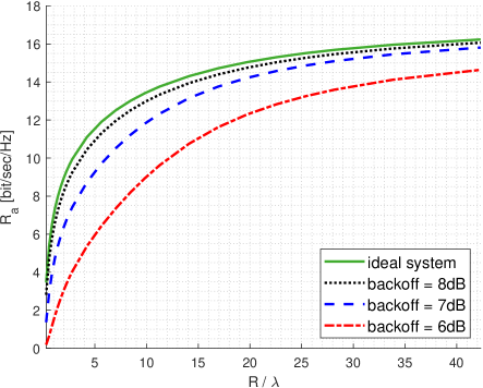
Figure 3: Achievable rate vs normalized LIS radius.

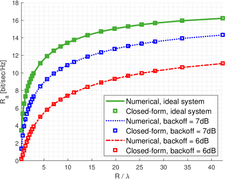
Figure 4: Numerical and Closed-form of achievable rate with perfect AGC vs normalized LIS radius.

VI-B Antenna and Panel selection

In Fig. 5, the performance of using the proposed optimal antenna selection in comparison to using the dominant antennas for signal reception is illustrated. We have used the 9th order distortion model for a GaN amplifier at $2.1$ GHz, as described in the previous section, with a $7$ dB of back-off. The UE transmit power is again selected such that the SNR at the center of LIS reaches $10$ dB, which corresponds to the respective value of $P_{\text{max}}$ in (11). We also assume that $N_{\text{max}}=\lceil 0.1N\rceil$ is selected as the antenna selection constraint. As we can see in Fig. 5, adopting the optimal antenna selection can improve the system performance significantly for medium to large LIS radius.

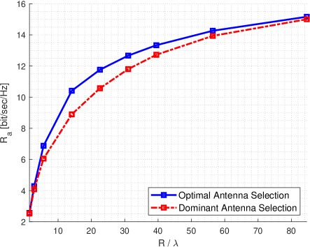
Figure 5: SE lower bound vs LIS radius with fixed back-off for optimal antenna selection solved from (41) and dominant antenna selection where the antennas with highest received power are selected.

In Fig. 6 we have illustrated the performance of panel-based LIS when adopting the proposed optimal panel selection versus the baseline approach corresponding to performing dominant panel selection, for different number of panels. The panel selection constraint in (46) is set to $N_{\text{max}}=\lceil 0.1N\rceil$. We also assume that each panel consists of $M=16$ antennas with $\lambda/2$ spacing, and the distance between the centers of adjacent panels is set to $\delta_{p}=5\lambda$. The same distortion model as in Fig. 5 is used for each antenna element of the LIS panels. We can see that there is a significant gain from applying the proposed optimal panel selection. In comparison to the results from Fig. 5 for antenna selection, the achievable performance gains are much higher, which implies that in the practical case of panel-based LIS deployment, it is even more important to consider the panel selection schemes in the presence of hardware distortion.

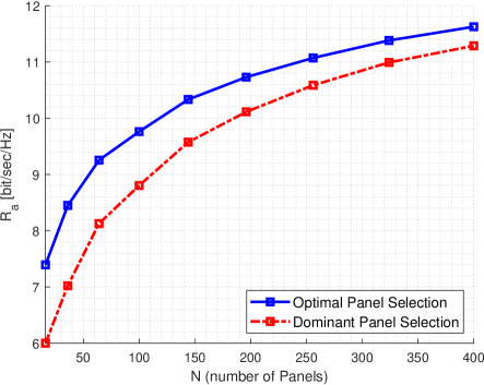
Figure 6: SE lower bound vs LIS radius with fixed back-off for optimal panel selection solved from (46) and dominant panel selection.

In Fig. 7, we have evaluated the performance of the approximate closed-form solution to the panel selection problem in comparison to the numerical optimal solution and the dominant panel selection. We have used the 3rd order non-linearity model for the hardware distortion as motivated in section V. The panel selection constraint and panel placement is the same as in Fig. 6. As we see, the optimal panel selection and closed-form panel selection outperform the dominant panel selection significantly, and the close-form panel selection performance is very close to the numerical optimal method, which implies that the proposed close-form solution is accurate enough to use in LIS panel selection problems with hardware distortion. In Fig. 8, we compare the performance gain of adopting such schemes for 3 different distance of the UE. We can see that the gain is higher if the UE is more into the near-field of the LIS, and it is still significant if the UE is placed at further distances.

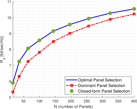
Figure 7: SE lower bound vs LIS radius with fixed back-off for optimal panel selection solved from (46) and dominant panel selection.

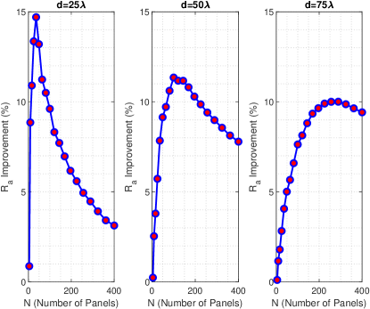
Figure 8: Percentage SE lower bound Improvement for different UE distances with fixed back-off for optimal panel selection and dominant panel selection.

To have a better understanding of the importance of panel selection in LIS applications, we study a practical panel-based LIS deployment scenario where a LIS consisting of $4\times 4$ panels covers the ceiling of a $6m\times 6m$ room. We consider two different room heights, $2.2m$ and $3m$, which are the typical numbers for ceiling heights in offices and residential buildings. The carrier frequency is set to $2.1$ GHz to match the hardware distortion measurements for the GaN amplifier from [20]. The distance between panels is $5\lambda$, the antenna spacing is $\lambda/2$, and the panel selection constraint is set to $N_{\text{max}}=\lceil 0.1N\rceil$. With these setup parameters, there are in total $N=64$ panels covering the ceiling and the selection schemes allocate $N_{\text{max}}=7$ panels to serve the UE, which is randomly located at the bottom of the room. In Fig. 9, we compare the CDF of the achievable rate for the case where the proposed optimal panel selection is adopted in comparison to the case where the dominant panels are assigned to the UE. We can see that for this scenario with typical setup parameters of a LIS indoor application, the gain from adopting the proposed panel selection is significant, and the LIS can provide a higher data rate with high probability just by adopting our proposed panel selection. We can also see that the data rate becomes worse in buildings with higher ceiling if the dominant panel selection is used, while the proposed panel selection can make the data rate more stable and higher, no matter if the ceiling is high or low.

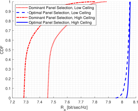
Figure 9: CDF of SE lower bound with fixed back-off for optimal panel selection and dominant panel selection for randomly located UE in a $6m\times 6m$ room.

VII Conclusion

In this paper, we have studied the impact of hardware distortion when considering LIS implementations with non-ideal RX-chains. We have derived analytical expressions for the SNDR considering the memory-less polynomial model for non-ideal hardware at the RX-chains. Such expressions enabled us to evaluate the performance of the LIS with hardware distortion when scaling up the system. We observe that the hardware quality can effectively limit the system performance even for extremely large LISs. We have also proposed antenna selection schemes for LIS and we have shown that adopting such schemes can improve the performance significantly. We also consider a more practical case where the LIS is deployed as a grid of multi-antenna panels, and define panel selection problems to improve the system performance. For the special case of 3rd-order nonlinear model, we have introduced a close-form panels selection solution, which can be exploited to efficiently switch panels with near-optimum performance.

Appendix A Proof of Lemmas

A-1 Proof of Lemma II.1

Considering the memory-less polynomial model (4) with $x\sim\mathcal{CN}(0,P)$, we first calculate $\mathbb{E}\left[y\bar{x}\right]$ as

$$\mathbb{E}\left[y\bar{x}\right]=\mathbb{E}\left[\sum_{k=0}^{L-1}a_{2k+1}x|x|^{2k}\bar{x}\right]=\sum_{k=0}^{L-1}a_{2k+1}\mathbb{E}\left[|x|^{2(k+1)}\right],$$ (55)

where the term $|x|^{2}$ is a Rayleigh variable, with $\mathbb{E}|x|^{2}=P$. The $(k+1)$’th moment of this Rayleigh variable is given by

$$\mathbb{E}\left[|x|^{2(k+1)}\right]=P^{k+1}\Gamma\left[1+(k+1)\right]=P^{k+1}(k+1)!,$$ (56)

which is replaced in (55) to find $g$ as

$$g=\frac{\mathbb{E}\left[y\bar{x}\right]}{\mathbb{E}\left[|x|^{2}\right]}=\sum_{k=0}^{L-1}a_{2k+1}(k+1)!~{}P^{k}.$$ (57)

In order to find $C_{\eta\eta}$, we need to calculate $C_{yy}$, which is given by

$$\mathbb{E}\left[y\bar{y}\right]=\mathbb{E}\left[\sum_{m=0}^{L-1}a_{2m+1}x|x|^{2m}\sum_{n=0}^{L-1}\bar{a}_{2n+1}\bar{x}|x|^{2n}\right],$$ (58)

which can be simplified by a change of variable and considering the moments of a Rayleigh variable to get

$$\mathbb{E}\left[y\bar{y}\right]=\sum_{k=1}^{2L-1}\left(k!~{}P^{k}\sum_{i=1}^{k}a_{2i-1}\bar{a}_{2k-2i+1}\right).$$ (59)

A-2 Proof of Lemma III.1

From (III) and (22), we need to calculate the following integrals,

$$\frac{d}{2}\int_{r=0}^{R}\frac{1}{(d^{2}+r^{2})^{\frac{3}{2}}}rdr,$$ (60)

$$\frac{d^{2}}{8\pi}\int_{r=0}^{R}\frac{1}{(d^{2}+r^{2})^{3}}rdr,$$ (61)

where we have simplified the phase part with a $2\pi$ factor before the integrals. By a change in variable as, $x=r^{2}$ and $rdr=\frac{1}{2}dx$, while using the following indefinite integral formulas,

$$\int\frac{1}{(d^{2}+x)^{\frac{3}{2}}}dx=\frac{-2}{\sqrt{d^{2}+x}},$$ (62)

$$\int\frac{1}{(d^{2}+x)^{3}}dx=\frac{-\frac{1}{2}}{(d^{2}+x)^{2}},$$ (63)

we can find the results in (23) and (24), and a simple factorization gives $\eqref{Riemannform3}$.

Appendix B Algorithms

Algorithm 1 provides a simple low-complexity numerical method to solve (31), where the accuracy of the solution depends on the number of iterations, $T$.

Algorithm 1 Numerical Method to solve (31)

  

  Define:  $R_{\mathrm{ub}}=$ (37),  $R_{\mathrm{lb}}=$ (38),  $\Delta=R_{\mathrm{ub}}-R_{\mathrm{lb}}$,  $R_{\text{opt}}=R_{\mathrm{lb}}$, $R_{\text{new}}=R_{\mathrm{lb}}$,  $T\in\mathcal{N}$ where $T>>1$.

  for $t=1$ to $T$:

        Calculate $\gamma$ from (31) for $R=R_{\text{new}}$

       if $\gamma\geq\gamma_{0}$:

           $R_{\text{opt}}=R_{\text{new}}$

           break

       else:

           $R_{\text{new}}=R_{\text{lb}}+\frac{t}{T}\Delta$

       endif

  endfor

Algorithm 2 can be used to find a sub-optimal solution to the optimization problem (44). By selecting a sufficiently large value for $T$, the sub-optimal solution from this algorithm can approach the optimal solution.

Algorithm 2 Sub-Optimal Solution to Problem (44)

  

  Define: $\tilde{R}=NA/\pi$, $r_{0}=0$, $R_{0}=\sqrt{N_{\text{max}}A/\pi}$, $\gamma_{0}=$ (26) with $R=R_{0}$, $r_{\text{opt}}=0$, $R_{\text{opt}}=R_{0}$, $\gamma_{\text{opt}}=\gamma_{0}$, $T\in\mathcal{N}$ where $T>>1$.

  for $t=1$ to $T$:

       $r_{\text{new}}=\frac{t}{T}\sqrt{\tilde{R}^{2}-N_{\text{max}}A/pi}$,

       $R_{\text{new}}=\sqrt{N_{\text{max}}A/\pi+r_{\text{opt}}^{2}}$,

       $\gamma_{\text{new}}=$ (44) with $r=r_{\text{new}}$ and $R=R_{\text{new}}$,

       if $\gamma<\gamma_{\text{opt}}$:

           break

       else:

           $r_{\text{opt}}=r_{\text{new}}$,

           $R_{\text{opt}}=R_{\text{new}}$,

           $\gamma_{\text{opt}}=\gamma_{\text{new}}$,

       endif

  endfor

References

- [1] S. Hu, F. Rusek, and O. Edfors, “Beyond massive MIMO: The potential of data transmission with large intelligent surfaces,” IEEE Transactions on Signal Processing, vol. 66, no. 10, pp. 2746–2758, 2018.
- [2] ——, “Beyond massive MIMO: The potential of positioning with large intelligent surfaces,” IEEE Transactions on Signal Processing, vol. 66, no. 7, pp. 1761–1774, 2018.
- [3] C. Huang, S. Hu, G. C. Alexandropoulos, A. Zappone, C. Yuen, R. Zhang, M. D. Renzo, and M. Debbah, “Holographic MIMO surfaces for 6G wireless networks: Opportunities, challenges, and trends,” IEEE Wireless Communications, vol. 27, no. 5, pp. 118–125, 2020.
- [4] E. Björnson and L. Sanguinetti, “Power scaling laws and near-field behaviors of massive MIMO and intelligent reflecting surfaces,” IEEE Open Journal of the Communications Society, vol. 1, pp. 1306–1324, 2020.
- [5] J. V. Alegría and F. Rusek, “Achievable rate with correlated hardware impairments in large intelligent surfaces,” in 2019 IEEE 8th International Workshop on Computational Advances in Multi-Sensor Adaptive Processing (CAMSAP), 2019, pp. 559–563.
- [6] E. G. Larsson, O. Edfors, F. Tufvesson, and T. L. Marzetta, “Massive MIMO for next generation wireless systems,” IEEE Communications Magazine, vol. 52, no. 2, pp. 186–195, 2014.
- [7] A. Pereira, F. Rusek, M. Gomes, and R. Dinis, “Deployment strategies for large intelligent surfaces,” IEEE Access, vol. 10, pp. 61 753–61 768, 2022.
- [8] F. Rusek, D. Persson, B. K. Lau, E. G. Larsson, T. L. Marzetta, O. Edfors, and F. Tufvesson, “Scaling up MIMO: Opportunities and challenges with very large arrays,” IEEE Signal Processing Magazine, vol. 30, no. 1, pp. 40–60, 2013.
- [9] C. Mollén, U. Gustavsson, T. Eriksson, and E. G. Larsson, “Impact of spatial filtering on distortion from low-noise amplifiers in massive MIMO base stations,” IEEE Transactions on Communications, vol. 66, no. 12, pp. 6050–6067, 2018.
- [10] H. Zhao, J. C. G. Diaz, and S. Hoyos, “Multi-channel receiver nonlinearity cancellation using channel speculation passing algorithm,” IEEE Transactions on Circuits and Systems II: Express Briefs, vol. 69, no. 2, pp. 599–603, 2022.
- [11] J. Marttila, M. Allén, M. Kosunen, K. Stadius, J. Ryynänen, and M. Valkama, “Reference receiver enhanced digital linearization of wideband direct-conversion receivers,” IEEE Transactions on Microwave Theory and Techniques, vol. 65, no. 2, pp. 607–620, 2017.
- [12] M. Sarajlić, A. Sheikhi, L. Liu, H. Sjöland, and O. Edfors, “Power scaling laws for radio receiver front ends,” IEEE Transactions on Circuits and Systems I: Regular Papers, vol. 68, no. 5, pp. 2183–2195, 2021.
- [13] A. Sheikhi, F. Rusek, and O. Edfors, “Massive MIMO with per-antenna digital predistortion size optimization: Does it help?” in ICC 2021 - IEEE International Conference on Communications, 2021, pp. 1–6.
- [14] A. Sheikhi and O. Edfors, “Machine learning based digital pre-distortion in massive MIMO systems: Complexity-performance trade-offs,” in 2023 IEEE Wireless Communications and Networking Conference (WCNC), 2023, pp. 1–6.
- [15] H. Tataria, F. Tufvesson, and O. Edfors, “Real-time implementation aspects of large intelligent surfaces,” in ICASSP 2020 - 2020 IEEE International Conference on Acoustics, Speech and Signal Processing (ICASSP), 2020, pp. 9170–9174.
- [16] J. Rodríguez Sánchez, F. Rusek, O. Edfors, and L. Liu, “Distributed and scalable uplink processing for LIS: Algorithm, architecture, and design trade-offs,” IEEE Transactions on Signal Processing, vol. 70, pp. 2639–2653, 2022.
- [17] O. T. Demir and E. Bjornson, “The bussgang decomposition of nonlinear systems: Basic theory and MIMO extensions [lecture notes],” IEEE Signal Processing Magazine, vol. 38, no. 1, pp. 131–136, 2021.
- [18] ——, “Channel estimation in massive MIMO under hardware non-linearities: Bayesian methods versus deep learning,” IEEE Open Journal of the Communications Society, vol. 1, pp. 109–124, 2020.
- [19] T. Schenk, RF imperfections in high-rate wireless systems: impact and digital compensation. Springer Science & Business Media, 2008.
- [20] “Further elaboration on PA models for NR,” document 3GPP TSG-RAN WG4, R4-165901, Ericsson, Stockholm, Sweden, Aug. 2016.
- [21] E. Bjornson, J. Hoydis, M. Kountouris, and M. Debbah, “Massive MIMO systems with non-ideal hardware: Energy efficiency, estimation, and capacity limits,” IEEE Transactions on Information Theory, vol. 60, no. 11, pp. 7112–7139, 2014.
- [22] E. Björnson, L. Sanguinetti, and J. Hoydis, “Hardware distortion correlation has negligible impact on UL massive MIMO spectral efficiency,” IEEE Transactions on Communications, vol. 67, no. 2, pp. 1085–1098, 2019.
- [23] M. Taylor, Measure Theory and Integration, ser. Graduate studies in mathematics. American Mathematical Society, 2006.
- [24] D. Dardari, “Communicating with large intelligent surfaces: Fundamental limits and models,” IEEE Journal on Selected Areas in Communications, vol. 38, no. 11, pp. 2526–2537, 2020.
- [25] G. Cardano, T. R. Witmer, and O. Ore, The rules of algebra: Ars Magna. Courier Corporation, 2007, vol. 685.
- [26] B. Hassibi and B. Hochwald, “How much training is needed in multiple-antenna wireless links?” IEEE Transactions on Information Theory, vol. 49, no. 4, pp. 951–963, 2003.