Robust multimode interference and conversion in topological unidirectional surface magnetoplasmons: supplemental document

Supplementary Material 1: Derivation of the analytic dispersion

Here, we solve the dispersion relation of the SMP in a metal-YIG-dielectric-YIG-metal structure under two opposite static magnetic fields, as shown in Fig. (1a) of the main text. This waveguide only supports the TE mode ($E_{x}$ = $E_{y}$ = $H_{z}$ = 0), which satisfies the Maxwell’s equations: $\nabla\times\bm{E}=i\omega\mu_{0}\bm{\mu}^{\pm}_{m}\bm{H}$ and $\nabla\times\bm{H}=-i\omega\varepsilon\varepsilon_{0}\bm{E}$. By substituting $\bm{\mu}^{\pm}_{m}$ (Eq. 1 in the main text), we can write all the scalar equations as

$$\dfrac{\partial E_{z}}{\partial y}=i\omega\mu_{0}(\mu_{1}H_{x}+i\mu_{2}H_{y})$$ (1)

$$- \dfrac{\partial E_{z}}{\partial x}=i\omega\mu_{0}(\mu_{1}H_{y}-i\mu_{2}H_{x})$$ (2)

$$\dfrac{\partial H_{y}}{\partial x}-\dfrac{\partial H_{x}}{\partial y}=-i\omega\varepsilon_{0}\varepsilon E_{z}$$ (3)

in the upper YIG layer, while the equations for the lower YIG layer can be obtained by replacing $\mu_{1}^{\prime}$ and $\mu_{2}^{\prime}$ with $\mu_{1}$ and $\mu_{2}$ in the Eq. (S1) and (S2). In the dielectric layer, $\mu_{1}=1$ and $\mu_{2}=0$. Considering plane waves, the electric field component $E_{z}$ is expressed as

$$\bm{E_{z1}} =(A_{1}e^{-{\alpha_{1}}y}+A_{2}e^{{\alpha_{1}}y})e^{i(kx-\omega t)},\quad y\in\scriptstyle{\left[\frac{h}{2},\frac{h}{2}+d\right)}$$

$$\bm{E_{z2}} =(B_{1}e^{-\alpha_{r}y}+B_{2}e^{\alpha_{r}y})e^{i(kx-\omega t)},\quad y\in\scriptstyle{\left[-\frac{h}{2},\frac{h}{2}\right)}$$ (4)

$$\bm{E_{z3}} =(C_{1}e^{-\alpha_{2}y}+C_{2}e^{\alpha_{2}y})e^{i(kx-\omega t)},\quad y\in\scriptstyle{\left[-\frac{h}{2}-d,-\frac{h}{2}\right)}$$

for the upper YIG layer, middle dielectric layer and lower YIG layer, respectively, where $A_{1}$, $A_{2}$, $B_{1}$, $B_{2}$, $C_{1}$ and $C_{2}$ are the amplitude of the field. Note that the attenuation coefficients (${\alpha_{1}}$, ${\alpha_{r}}$, ${\alpha_{2}}$) and the other parameters (such as: $k$, $\mu_{v}$, $\mu_{v}^{\prime}$) are presented in the main text.

By combining Eq. (S1) and (S2), the nonzero components ($H_{x}$, $H_{y}$) of the magnetic field can be directly derived from $E_{z}$, thus $H_{x}$ for three layers can be obtained by substituting $E_{z1}$, $E_{z2}$ and $E_{z3}$ as

$$\bm{H_{x1}}=\dfrac{i}{\mu_{v}\mu_{0}\omega}\left[(k\dfrac{\mu_{2}}{\mu_{1}}+\alpha_{1})A_{1}e^{-\alpha_{1}y}+(k\dfrac{\mu_{2}}{\mu_{1}}-\alpha_{1})A_{2}e^{\alpha_{1}y}\right]e^{i(kx-\omega t)}$$

$$\bm{H_{x2}}=\dfrac{i\alpha_{r}}{\mu_{0}\omega}(B_{1}e^{-\alpha_{r}y}-B_{2}e^{\alpha_{r}y})e^{i(kx-\omega t)}$$ (5)

$$\bm{H_{x3}}=\dfrac{i}{\mu_{v}^{\prime}\mu_{0}\omega}\left[(-k\dfrac{\mu^{\prime}_{2}}{\mu^{\prime}_{1}}+\alpha_{2})C_{1}e^{-\alpha_{2}y}-(k\dfrac{\mu_{2}^{\prime}}{\mu_{1}^{\prime}}+\alpha_{2})C_{2}e^{\alpha_{2}y}\right]e^{i(kx-\omega t)}$$

According to the boundary conditions of electric and magnetic fields, $E_{z}$ and $H_{x}$ are continuous at the YIG-dielectric interfaces $y=\pm\frac{h}{2}$, while the electric field $E_{z}$ is zero at the YIG-metal interfaces $y=0$, where the metal is assumed to be a perfect electric conductor (PEC). Therefore, we obtain six boundary equations as follows

$$\begin{cases}\text{\char 172}\quad E_{z1}\mid_{y=\frac{h}{2}+d}=0\quad(\text{PEC boundary})\\[6.0pt] \text{\char 173}\quad E_{z1}\mid_{y=\frac{h}{2}}=E_{z2}\mid_{y=\frac{h}{2}}\\[6.0pt] \text{\char 174}\quad H_{x1}\mid_{y=\frac{h}{2}}=H_{x2}\mid_{y=\frac{h}{2}}\\[6.0pt] \text{\char 175}\quad E_{z2}\mid_{y=-\frac{h}{2}}=E_{z3}\mid_{y=-\frac{h}{2}}\\[6.0pt] \text{\char 176}\quad H_{x2}\mid_{y=-\frac{h}{2}}=H_{x3}\mid_{y=-\frac{h}{2}}\\[6.0pt] \text{\char 177}\quad E_{z3}\mid_{y=-\frac{h}{2}-d}=0\quad(\text{PEC boundary})\end{cases}$$ (6)

By substituting $E_{z}$ and $H_{x}$ from Eqs. (S4) and (S5) into Eqs. (S6), we obtain

$$\begin{cases}\text{\char 172}\quad A_{1}e^{-\alpha_{1}(\frac{h}{2}+d)}+A_{2}e^{\alpha_{1}(\frac{h}{2}+d)}=0\\[6.0pt] \text{\char 173}\quad A_{1}e^{-\alpha_{1}\frac{h}{2}}+A_{2}e^{\alpha_{1}\frac{h}{2}}=B_{1}e^{-\alpha_{1}\frac{h}{2}}+B_{2}e^{\alpha_{1}\frac{h}{2}}\\[6.0pt] \text{\char 174}\quad\dfrac{1}{\mu_{v}}\left[(k\dfrac{\mu_{2}}{\mu_{1}}+\alpha_{1})A_{1}e^{-\alpha_{1}\frac{h}{2}}+(k\dfrac{\mu_{2}}{\mu_{1}}-\alpha_{1})A_{2}e^{\alpha_{1}\frac{h}{2}}\right]=\alpha_{r}(B_{1}e^{-\alpha_{r}\frac{h}{2}}-B_{2}e^{\alpha_{r}\frac{h}{2}})\\[6.0pt] \text{\char 175}\quad B_{1}e^{\alpha_{r}\frac{h}{2}}+B_{2}e^{-\alpha_{r}\frac{h}{2}}=C_{1}e^{\alpha_{2}\frac{h}{2}}+C_{2}e^{-\alpha_{2}\frac{h}{2}}\\[6.0pt] \text{\char 176}\quad\dfrac{1}{\mu_{v}^{\prime}}\left[(-k\dfrac{\mu^{\prime}_{2}}{\mu^{\prime}_{1}}+\alpha_{2})C_{1}e^{\alpha_{2}\frac{h}{2}}-(k\dfrac{\mu_{2}^{\prime}}{\mu_{1}^{\prime}}+\alpha_{2})C_{2}e^{-\alpha_{2}\frac{h}{2}}\right]=\alpha_{r}(B_{1}e^{\alpha_{r}\frac{h}{2}}-B_{2}e^{-\alpha_{r}\frac{h}{2}})\\[6.0pt] \text{\char 177}\quad C_{2}+C_{1}e^{2\alpha_{2}(\frac{h}{2}+d)}=0\end{cases}$$ (7)

Finally, by eliminate the coefficients $A_{1},A_{2},B_{1},B_{2},C_{1},C_{2}$ from the six boundary equations in Eqs. (S7), we can solve for the dispersion relation of the SMP

$$e^{2\alpha_{r}h}=\dfrac{\left[1-\dfrac{1}{\alpha_{r}\mu_{v}}(k\dfrac{\mu_{2}}{\mu_{1}}+\dfrac{\alpha_{1}}{\tanh(\alpha_{1}d)})\right]\left[1-\dfrac{1}{\alpha_{r}\mu_{v}^{\prime}}(k\dfrac{\mu_{2}^{\prime}}{\mu_{1}^{\prime}}+\dfrac{\alpha_{2}}{\tanh(\alpha_{2}d)})\right]}{\left[1+\dfrac{1}{\alpha_{r}\mu_{v}}(k\dfrac{\mu_{2}}{\mu_{1}}+\dfrac{\alpha_{1}}{\tanh(\alpha_{1}d)})\right]\left[1+\dfrac{1}{\alpha_{r}\mu_{v}^{\prime}}(k\dfrac{\mu_{2}^{\prime}}{\mu_{1}^{\prime}}+\dfrac{\alpha_{2}}{\tanh(\alpha_{2}d)})\right]}.$$ (8)

Simplifying the dispersion equation, Eq. (S8) becomes

$$e^{2\alpha_{r}h}=\frac{\left(1-\dfrac{M}{\alpha_{r}\mu_{v}}\right)\left(1-\dfrac{N}{\alpha_{r}\mu_{v}^{\prime}}\right)}{\left(1+\dfrac{M}{\alpha_{r}\mu_{v}}\right)\left(1+\dfrac{N}{\alpha_{r}\mu_{v}^{\prime}}\right)}$$ (9)

with $\bm{M}=k\dfrac{\mu_{2}}{\mu_{1}}+\dfrac{\alpha_{1}}{\tanh{\alpha_{1}d}}$ and $\bm{N}=k\dfrac{\mu_{2}^{\prime}}{\mu_{1}^{\prime}}+\dfrac{\alpha_{2}}{\tanh{\alpha_{2}d}}$, which corresponding Eq. 2 in the main text.

When considering a symmetry structure where $H_{1}=H_{2}$, we have $\alpha_{1}=\alpha_{2}$, $\mu_{2}=\mu_{2}^{\prime}$, $\mu_{1}=\mu_{1}^{\prime}$, and $\mu_{v}=\mu_{v}^{\prime}$. Thus, $M=N$ in Eq. (S9), and we obtain

$$e^{2\alpha_{r}h}=\left(\frac{1-\dfrac{M}{\alpha_{r}\mu_{v}}}{1+\dfrac{M}{\alpha_{r}\mu_{v}}}\right)^{2}$$ (10)

Obviously, there are two solutions in Eq. (S10). Combining these solutions with the formula of $tanh(x)=\dfrac{e^{x}-e^{-x}}{e^{x}+e^{-x}}$, we have

$$e^{\alpha_{r}h}=\frac{1+\tanh\left(\frac{\alpha_{r}h}{2}\right)}{1-\tanh\left(\frac{\alpha_{r}h}{2}\right)}=\pm\frac{1-\dfrac{M}{\alpha_{r}\mu_{v}}}{1+\dfrac{M}{\alpha_{r}\mu_{v}}}$$ (11)

From Eq.(S10), the dispersion relation of SMP can be simplified

$$k\dfrac{\mu_{2}}{\mu_{1}}+\dfrac{\alpha_{1}}{\tanh{\alpha_{1}d}}+\alpha_{r}\mu_{\rm{v}}{\rm{tanh}}\left(\dfrac{\alpha_{r}h}{2}\right)=0\quad(ES)$$ (12a)

$$k\dfrac{\mu_{2}}{\mu_{1}}+\dfrac{\alpha_{1}}{\tanh{\alpha_{1}d}}+\alpha_{r}\mu_{\rm{v}}{\rm{coth}}\left(\dfrac{\alpha_{r}h}{2}\right)=0\quad(OS)$$ (12b)

for the even-symmetric (ES) and odd-symmetric (OS) modes, respectively, which correspond Eq. 3 in the main text.

Supplementary Material 2: the waveguide properties for different parameters

In the main text, we use fixed values for parameters (such as loss and magnetic field) as examples to investigate the performance of the waveguide. Here, we analyze the impact of varying these parameter values on the waveguide characteristics.

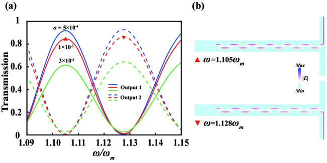
Figure 1: The effect of YIG loss $\alpha$ on the USMMI-based splitter. (a) Transmission coefficients of the symmetric splitter as a function of $\omega$ for different values of $\alpha$. (b) Simulated $E$-field amplitude for $\alpha=1\times 10^{-3}$ at $\omega=1.105\omega_{m}$ and $\omega=1.128\omega_{m}$. The other parameters are the same as in Fig. 2 of the main text.

We first investigate the impact of YIG loss on the USMMI-based splitter. Given that the YIG material used in different experiments exhibits varying loss coefficients [1, 2], we analyze the transmission coefficients of the symmetric splitter ($H_{1}=H_{2}=893$ G) under different YIG loss coefficients, as shown in Fig. 1(a). As the loss varies from $\alpha=3\times 10^{-5}$ to $\alpha=3\times 10^{-3}$, the splitting ratio of each output can be tuned by adjusting the frequencies, while the total transmission decreases with $\alpha$. Fig. 1(b) shows the simulated E-field amplitudes for $\alpha=1\times 10^{-3}$. Similar to the results for $\alpha=3\times 10^{-5}$ shown in Fig. 2(d) of the main text, the unidirectional SMP propagates upward and downward at $\omega=1.105\omega_{m}$ and $1.128\omega_{m}$, as expected. Therefore, we conclude that the frequency splitter based on USMMI can be achieved for different YIG loss values. It should be noted that for a larger loss of $\alpha=3\times 10^{-3}$, non-zero power is clearly observed at $\omega=1.105\omega_{m}$, while the power in the downward port is nearly zero for $\alpha=1\times 10^{-3}$, as indicated by the dashed line in Fig. 1(a). To further investigate this phenomenon, we independently excite the odd and even modes and calculate their transmission efficiencies ($\eta_{odd}$ and $\eta_{even}$) over a distance of $\lambda_{m}$. Here, we take $\omega=1.1\omega_{m}$ as an example. We find that $\eta_{odd}=99.6\%$ and $\eta_{even}=99.9\%$ for $\alpha=3\times 10^{-5}$, $\eta_{odd}=92.9\%$ and $\eta_{even}=98.1\%$ for $\alpha=5\times 10^{-4}$, $\eta_{odd}=86.3\%$ and $\eta_{even}=96.2\%$ for $\alpha=1\times 10^{-3}$, and $\eta_{odd}=64.2\%$ and $\eta_{even}=89.0\%$ for $\alpha=3\times 10^{-3}$. The results indicate that non-zero power arises from the significant difference in transmission losses between the odd and even modes at higher YIG loss values, while the difference in transmission losses remains smallish for reasonable YIG losses, enabling near 0 to 1 splitting performance.

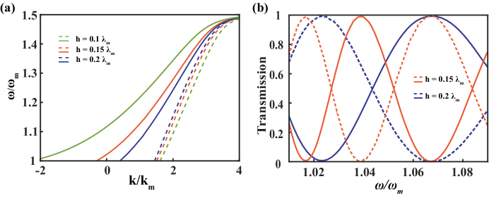
Figure 2: The impact of the dielectric width $h$. (a) The dispersions of odd (solid lines) and even (dashed lines) SMP modes vary with different $h$ in the whole USMMI band. (b) Transmission coefficients of the symmetric splitter as a function of $\omega$ for two different values of $h$: $0.15\lambda_{m}$ and $0.2\lambda_{m}$, where the solid and dashed lines represent the transmission in the upper and lower ports of the splitter.

The impact of the dielectric width $h$ on the properties of the waveguide is further explored. Figure 2(a) shows the calculated dispersion curves for the SMP at various $h$ values using MATLAB software. It can be observed that as $h$ increases from $h=0.1\lambda_{m}$ to $h=0.2\lambda_{m}$, the odd and even modes supported by the SMP waveguide gradually converge; however, the unidirectional propagation bands remain consistent within the range of [$\omega_{m}$, $1.5\omega_{m}$]. By maintaining all other parameters consistent with those in Fig. 2(d) of the main text, we calculated the transmission coefficients for different $h$ values. As shown in Fig. 2(b), the beam-splitting performance remains nearly between 0 and 1 despite changes in $h$, when the frequency changes from $1.01\omega_{m}$ to $1.09\omega_{m}$. Due to variations in $h$, the beat length $L_{\pi}$ at the same frequency changes, resulting in different splitting ratios at the same frequency. The results demonstrate that a frequency-tunable splitter can be achieved for different dielectric thicknesses.

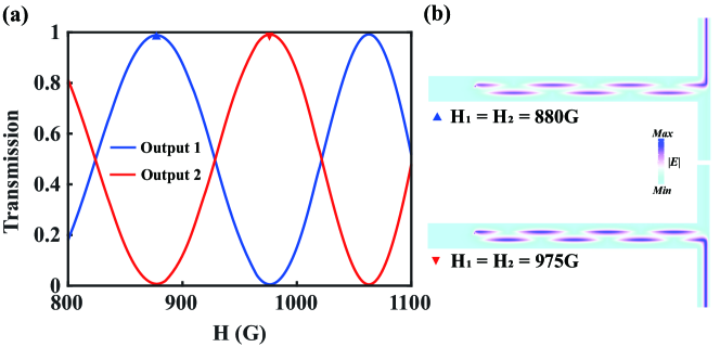
Figure 3: Magnetically controllable splitter. (a) Transmission coefficient as a function of the magnetic field for $H_{1}=H_{2}$. (b) Simulated $E$-field amplitude for $H_{1}=H_{2}=880\,\text{G}$ and $H_{1}=H_{2}=975\,\text{G}$, clearly demonstrating that the energy is almost entirely directed to the upper port (output 1) and the lower port (output 2), respectively. The working frequency is $\omega=1.1\omega_{m}$.

It should be noted that, for our proposed waveguide, a magnetically tunable power splitter based on USMMI can be realized at a fixed frequency. To verify this, we calculate the transmission coefficients of the symmetric splitter ($H_{1}=H_{2}$) as a function of the external magnetic field $H$, as shown in Fig. 3(a). Here, we choose a fixed frequency of $\omega=1.1\omega_{m}$ as an example. It is clearly shown that the beam splitting ratio can be achieved from 0 to 1 by changing the $H$ value from $880$ G to $975$ G. Figure 3(b) shows the simulated $E$-field amplitude for $H_{1}=H_{2}=880\,\text{G}$ and $H_{1}=H_{2}=975\,\text{G}$, clearly demonstrating that the energy is almost entirely directed to the upper port (output 1) and the lower port (output 2), respectively. Therefore, a magnetically controllable power splitter is realized using USMMI.

Finally, we compared our magnetized waveguide with a non-magnetized waveguide, as shown in Fig. S4. To investigate their robustness against defect, we introduced a square metallic obstacle with a length of 2 mm on the right side of the waveguide. Figures 4(a) and 4(b) show the simulated $E$-field results with and without the external magnetic field, respectively. In the full-wave simulations, a point source with $\omega=1.1\omega_{m}$ is used to excite the mode, marked by a red star. As seen in Fig. 4(a), the excited mode in our magnetized waveguide can only propagate forward, not backward, demonstrating its characteristic of unidirectional propagation without backscattering, even when the obstacle is introduced. In contrast, the mode in the non-magnetized waveguide can propagate both forward and backward, and strong backscattering occurs due to the obstacle, as shown in Fig. 4(b). To clearly illustrate this, Figures 4(c) and 4(d) show the $E$-field distributions along the upper YIG-air interface, with and without obstacles, respectively. As seen from the solid and dashed lines in Fig. 4(c), the field amplitudes on the left side of the obstacle completely overlap with and without the obstacle, and it recovers after passing through the obstacle, demonstrating the strong robustness of our magnetized waveguide. However, the non-magnetized waveguide exhibits a symmetric field distribution without the obstacle due to its reciprocal propagation (see the blue solid line in Fig. 4(d)), and significant changes occur in the distribution due to the strong backscattering from the obstacle (see the red dashed line in Fig. 4(d)). These results further validate the advantage of our structure in achieving robust topological unidirectional propagation without backscattering.

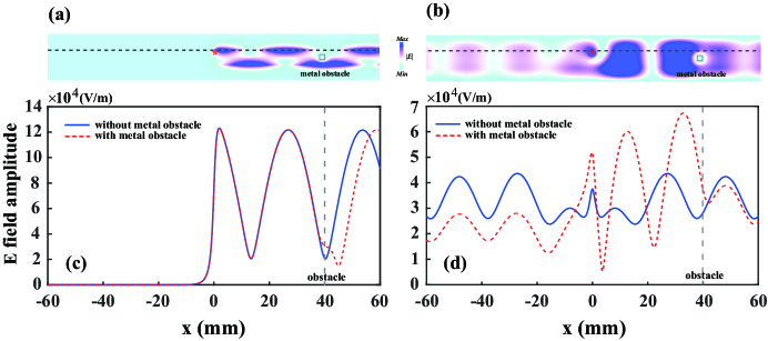
Figure 4: Comparison of the waveguide with (a, c) and without (b, d) external magnetic field. E-field distribution diagrams. (a) A unidirectional mode without backscattering. (b) A regular mode with strong backscattering. (c, d) The field distribution with (the red dashed lines) and without (the blue solid lines) a 2 mm square metallic obstacle along the YIG-air interface, indicated by the black dashed lines in (a) and (b). The red star shows the position of the point source. $H_{1}=H_{2}=893$ G, and $\omega=1.1\omega_{m}$.

References

• [1] W.Β Tang, M.Β Wang, S.Β Ma, etΒ al., β€œMagnetically controllable multimode interference in topological photonic crystals,” \JournalTitleLight: Science & Applications 13, 112 (2024).
• [2] W.Β Tong, J.Β Wang, J.Β Wang, etΒ al., β€œMagnetically tunable unidirectional waveguide based on magnetic photonic crystals,” \JournalTitleApplied Physics Letters 109, 053502 (2016).