Over-the-Air DPD and Reciprocity Calibration in Massive MIMO and Beyond

Abstract

In this paper we study an over-the-air (OTA) approach for digital pre-distortion (DPD) and reciprocity calibration in massive multiple-input-multiple-output systems. In particular, we consider a memory-less non-linearity model for the base station (BS) transmitters and propose a methodology to linearize the transmitters and perform the calibration by using mutual coupling OTA measurements between BS antennas. We show that by only using the OTA-based data, we can linearize the transmitters and design the calibration to compensate for both the non-linearity and non-reciprocity of BS transceivers effectively. This allows to alleviate the requirement to have dedicated hardware modules for transceiver characterization. Moreover, exploiting the results of the DPD linearization step, our calibration method may be formulated in terms of closed-form transformations, achieving a significant complexity reduction over state-of-the-art methods, which usually rely on costly iterative computations. Simulation results showcase the potential of our approach in terms of the calibration matrix estimation error and downlink data-rates when applying zero-forcing precoding after using our OTA-based DPD and calibration method.

I Introduction

Massive multiple-input multiple-output (MIMO) has been one of the main technologies in the development of the fifth-generation (5G) of wireless networks, by enabling significant improvement in network capacity and reliability [1, 2]. In the early stages of massive MIMO development, several proposals motivated the adoption of frequency-division duplexing (FDD) in massive MIMO deployments. While some advantages may arise from considering FDD [3], the over-head in downlink channel estimation is an important drawback which limits the system scalability. Therefore, time-division duplexing (TDD) is selected as the more viable approach for the deployment of massive MIMO in 5G and beyond, since it enables downlink channel estimation based on uplink channel state information (CSI) and channel reciprocity [4].

In ideal TDD systems, perfect channel reciprocity allows the base station (BS) to use the uplink (UL) CSI also for downlink (DL) precoding. However, in practical deployments, the difference in transmit (TX) and receive (RX) hardware may compromise this assumption [5]. To tackle this issue, reciprocity calibration methods are employed to compensate the difference in TX and RX hardware in DL precoding. There are several approaches for reciprocity calibration in massive MIMO systems. OTA-based reciprocity calibration methods relying on mutual-coupling measurements are specially promising since they do not require dedicated hardware for reciprocity calibration [6, 7]. Another challenge in implementing massive MIMO systems is the non-linear response of the transceivers. There are several methods to compensate the non-linearity effects, with per-antenna digital pre-distortion (DPD) being the most favorable option because of its effectiveness [8]. To perform the DPD, many approaches rely on input-output measurements of the amplifiers and analogue front-ends to design an inverse function for cancelling the non-linearity effects [8, 9, 10]. over-the-air (OTA)-based DPD approaches such as the methods based on wireless links with near-field or far-field probes have emerged as an efficient alternative to linearize the amplifiers by exploiting the OTA data [11].

In this paper, we propose a method exploiting OTA measurements of inter-antenna mutual couplings at the BS to perform both the DPD and reciprocity calibration. The reciprocity methods in the literature mostly rely on linear transceivers, i.e., modelled by a complex number [6, 5]. This assumption is not accurate in practical cases, especially when scaling up massive MIMO systems, which necessitates deploying less expensive non-linear components and low-end DPD modules. Therefore, we assume that the TX-chains in the BS are non-linear and we propose a method to linearize them based on mutual coupling measurements. Our approach relies on the same hardware available for OTA-based reciprocity calibration, which eliminates the need for excessive hardware resources to perform per-antenna DPD. We show that, once the transmitters are linearized through the OTA-based method, reciprocity calibration becomes even simpler than previous approaches, allowing for a significant complexity reduction over the methods in [6, 5]. Numerical results show that, although we consider non-linear TX-chains, the calibration matrix estimation error is fairly close to the Cramer-Rao Lower Bound (CRLB) for the method from [6]. We also evaluate the system performance in downlink data transmission using zero-forzing (ZF) precoding and show that the proposed calibration method can approach the optimal calibration performance for moderate values of signal to noise ratio (SNR).

II System Model

We consider a TDD massive MIMO scenario where an $M$-antenna BS serves $K\ll M$ user equipments through a narrow-band channel. We assume that the UE transceivers operate in the linear regime during UL and DL. The BS receivers are also assumed to operate in the linear regime for the UL, but the BS transmitters exhibit non-linear response for the DL.

II-A Uplink

The $M\times 1$ vector of received symbols at the BS during an UL transmission may be expressed as

$$\boldsymbol{y}_{\mathrm{B}}=\boldsymbol{H}_{\mathrm{UL}}\boldsymbol{s}_{\mathrm{U}}+\boldsymbol{n}_{\mathrm{B}},$$ (1)

where $\boldsymbol{s}_{\mathrm{U}}$ is the $K\times 1$ vector of input symbols to each UE TX-chain and $\boldsymbol{n}_{\mathrm{B}}\sim\mathcal{CN}(\boldsymbol{0},N_{0,\mathrm{B}}\boldsymbol{I}_{M})$ models the additive white Gaussian noise (AWGN) at the BS. The $M\times K$ channel matrix, is given by

$$\boldsymbol{H}_{\mathrm{UL}}=\boldsymbol{R}_{\mathrm{B}}\boldsymbol{H}\boldsymbol{T}_{\mathrm{U}},$$ (2)

where $\boldsymbol{R}_{\mathrm{B}}=\mathrm{diag}(r^{\mathrm{B}}_{1},\dots,r^{\mathrm{B}}_{M})$ and $\boldsymbol{T}_{\mathrm{U}}=\mathrm{diag}(t_{1}^{\mathrm{U}},\dots,t^{\mathrm{U}}_{K})$ are associated with the linear response of the BS receivers and the UE transmitters, respectively, and $\boldsymbol{H}$ corresponds to the $M\times K$ reciprocal propagation channel matrix [6].

The UL channel, which includes the effects of the UE transmitters and the BS receivers, is assumed to be perfectly estimated at the BS based on UL pilots transmitted by the UEs. Hence, perfect knowledge of $\boldsymbol{H}_{\mathrm{UL}}$ is available at the BS, allowing for effective implementation of linear processing techniques, e.g., ZF, linear minimum mean squared error (LMMSE), and maximum ratio combining (MRC), to estimate $\boldsymbol{s}_{\mathrm{U}}$. However, the diagonal entries of $\boldsymbol{T}_{\mathrm{U}}$ and $\boldsymbol{R}_{\mathrm{B}}$, which may take arbitrary complex numbers, are unknown since they can be affected by parameters such as temperature, hardware imperfections, etc.

II-B Downlink

During the DL transmission phase, the $K\times 1$ vector of symbols received at the UEs may be expressed as

$$\boldsymbol{y}_{\mathrm{U}}=\boldsymbol{R}_{\mathrm{U}}\boldsymbol{H}^{\mathrm{T}}\boldsymbol{f}(\boldsymbol{x}_{\mathrm{B}})+\boldsymbol{n}_{\mathrm{U}},$$ (3)

where $\boldsymbol{x}_{\mathrm{B}}$ is the $M\times 1$ vector of input symbols to each BS TX-chain, $\boldsymbol{n}_{\mathrm{U}}\sim\mathcal{CN}(\boldsymbol{0},\mathrm{diag}(N_{0,\mathrm{U}_{1}},\dots,N_{0,\mathrm{U}_{K}}))$ models the AWGN at the UEs, $\boldsymbol{R}_{\mathrm{U}}=\mathrm{diag}((r^{\mathrm{U}}_{1},\dots,r^{\mathrm{U}}_{K})$ is associated with the linear response of the UE receivers, while $\boldsymbol{f}:\mathbb{C}^{M\times 1}\rightarrow\mathbb{C}^{M\times 1}$ is a vector-valued function modeling the non-linear response of the BS TX-chains. We assume that the transmitted symbols are generated such that

$$\boldsymbol{x}_{\mathrm{B}}=\boldsymbol{g}(\boldsymbol{W}\boldsymbol{s}_{\mathrm{B}}),$$ (4)

where $\boldsymbol{s}_{\mathrm{B}}$ is the $K\times 1$ vector of symbols intended for the UEs, $\boldsymbol{W}$ is the $M\times K$ linear precoding matrix applied at the BS baseband unit (BBU), while $\boldsymbol{g}:\mathbb{C}^{M\times 1}\rightarrow\mathbb{C}^{M\times 1}$ is the non-linear vector-valued function associated to the DPD applied at each TX-chain.

Let us assume that the cross-talk between TX-chains is negligible so that $\boldsymbol{f}(\cdot)$, and correspondingly $\boldsymbol{g}(\cdot)$, are component-wise functions. Considering a third-order memory-less polynomial model [12], we express

$$f_{m}(\boldsymbol{x})=t^{\mathrm{B}}_{m}x_{m}+\beta_{m}x_{m}|x_{m}|^{2},\;\;\;\;\forall m\in\{1,\dots,M\},$$ (5)

where $t^{\mathrm{B}}_{m}$ and $\beta_{m}$ are two complex scalars characterizing the non-linear response of the $m$’th TX-chain at the BS. The BS TX-chain and UEs RX-chain responses are unknown in general, which means that the non-linear parameters $t^{\mathrm{B}}_{m}$ and $\beta_{m}$, as well as the diagonal entries of $\boldsymbol{R}_{\mathrm{U}}$, are unknown at the BS. Note that, unlike traditional work on reciprocity calibration [6], where $\boldsymbol{f}(\cdot)$ is associated to a linear transformation $\boldsymbol{T}_{B}=\mathrm{diag}(t^{\mathrm{B}}_{1},\dots,t^{\mathrm{B}}_{M})$, we cannot hereby define an aggregated DL channel matrix due to the non-linear nature of the TX-chains.

II-C Background: OTA Reciprocity Calibration

As mentioned earlier, previous work has addressed the problem of reciprocity calibration in massive MIMO assuming BS TX-chains that operate in the linear regime [6, 5]. Under such assumptions, we may define the DL channel matrix as

$$\boldsymbol{H}_{\mathrm{DL}}=\boldsymbol{R}_{\mathrm{U}}\boldsymbol{H}^{\mathrm{T}}\boldsymbol{T}_{\mathrm{B}},$$ (6)

which may be also derived from the presented system model, assuming $\beta_{m}=0$ in (5). The main goal of reciprocity calibration methods as the ones in [6] is to estimate the reciprocity matrix, defined as

$$\boldsymbol{C}=\boldsymbol{T}_{\mathrm{B}}\boldsymbol{R}_{\mathrm{B}}^{-1}.$$ (7)

The reason is that, if we have knowledge of $\boldsymbol{C}$, we can transform the known UL channel matrix into

$$\widetilde{\boldsymbol{H}}_{\mathrm{DL}} =(\boldsymbol{C}\boldsymbol{H}_{\mathrm{UL}})^{\mathrm{T}}$$ (8)

$$=\boldsymbol{T}_{\mathrm{U}}\boldsymbol{H}^{\mathrm{T}}\boldsymbol{T}_{\mathrm{B}}.$$

Note that $\widetilde{\boldsymbol{H}}_{\mathrm{DL}}$ corresponds to $\boldsymbol{H}_{\mathrm{DL}}$ up to an unknown $K\times K$ diagonal matrix, namely $\boldsymbol{D}=\boldsymbol{T}_{\mathrm{U}}\boldsymbol{R}_{\mathrm{U}}^{-1}$, multiplied from the left. Hence, $\widetilde{\boldsymbol{H}}_{\mathrm{DL}}$ can be effectively used for linear precoding, with the only caveat that the symbols received by the UEs would end up multiplied by an unknown scalar, which has negligible impact on system performance [13]. We may thus ignore the non-reciprocity associated to the UEs hardware, modeled by $\boldsymbol{R}_{\mathrm{U}}$ and $\boldsymbol{T}_{\mathrm{U}}$, and focus on characterizing the non-reciprocity associated to the BS.

An important advantage of the OTA-based calibration methods which are based on mutual coupling measurements is that they avoid the need for dedicated hardware to characterize the linear response of each transceiver chain, and can improve the cost-efficiency of massive MIMO systems [6, 5]. Similarly, we can argue that having dedicated hardware to perform DPD may compromise the cost-efficiency of MIMO systems with increasing number of antennas, e.g., massive MIMO and beyond. Thus, we next propose a method to jointly characterize the non-linear response of the BS TX-chains, as well as the resulting reciprocity matrix, so as to be able to suitably design $\boldsymbol{g}(\cdot)$ and $\boldsymbol{W}$ (given $\boldsymbol{H}_{\mathrm{UL}}$) for effectively serving the UEs in the DL.

III OTA DPD and reciprocity calibration

Our proposed OTA-based solution may be divided into three stages:

• First, the non-linear response of the BS TX-chains, associated to $\boldsymbol{f}(\cdot)$, is estimated based on OTA mutual coupling measurements.

• Second, the DPD, associated to $\boldsymbol{g}(\cdot)$, is designed based on the estimated non-linear response.

• Third, reciprocity calibration is performed based on the DPD-linearized BS TX-chains, after which effective DL precoding, associated to $\boldsymbol{W}$, would become available at the BS.

III-A OTA non-linearity characterization

In this stage each BS antenna transmits $N_{\mathrm{dpd}}\geq 2$ inter-antenna pilot signals to estimate the non-linearity parameters. The signal received at the $j$’th antenna when the $\ell$’th pilot, $\ell\in\{1,\dots,N_{\text{dpd}}\}$, is transmitted by the $i$’th antenna may be expressed as

$$y_{ij,\ell}=h_{ij}r_{j}\left(t_{i}x_{i,\ell}+\beta_{i}x_{i,\ell}|x_{i,\ell}|^{2}\right)+n_{ij,\ell},$$ (9)

where $h_{ij}$ is the mutual coupling gain between antennas $i$ and $j$, which is assumed fixed and known at the BS, $x_{i,\ell}$ is the $\ell$’th pilot symbol transmitted by the $i$’th antenna, and $n_{ij,\ell}\sim\mathcal{CN}(0,N_{0})$ models the measurement noise. Note that we have removed the superscript B from the parameters $r_{j}$ and $t_{i}$ for notation convenience since, as previously reasoned, we may focus on the non-reciprocity associated to the BS.

For each pair of non-linearity parameters associated to one TX-chain, there are $M-1$ relevant DPD measurements per pilot transmission, i.e., all of those originated in the same antenna, but received at different antennas. Thus, each of these measurements would share the same $t_{i}$ and $\beta_{i}$ in (9), but they would be related to a different complex gain $r_{j}$, associated to the linear response of RX-chain from the respective receiving antenna. Since the complex gains $r_{j}$ are unknown, it is not possible to directly estimate the non-linearity parameters $t_{i}$ and $\beta_{i}$ from this dataset. We may, however, combine the $M-1$ measurements by averaging them after compensating for the known mutual coupling gains, so as to reduce the uncertainty, as well as the resulting noise. The combined measurements are then given by

$$\tilde{y}_{i,\ell} =\frac{1}{M-1}\sum_{j\neq i}\frac{y_{ij,\ell}}{h_{ij}}$$ (10)

$$={q_{i}}(t_{i}x_{i,\ell}+\beta_{i}x_{i,\ell}|x_{i,\ell}|^{2})+\tilde{n}_{i,\ell},$$

where the uncertainty is now captured in the unknown parameter $q_{i}$, given by

$$q_{i}=\frac{1}{M-1}\sum_{j\neq i}r_{j}.$$ (11)

Note that one could also explore alternative optimized combinations to the simple average in (10). For example, a weighted summation could be optimized assuming a specific model for $h_{ij}$ or a concrete probability distribution for $r_{j}$, which are out of scope for this paper and can be considered in future work.

The $N_{\text{dpd}}\times 1$ data vector $\tilde{\boldsymbol{y}}_{i}=[\tilde{y}_{i,1},\dots,\tilde{y}_{i,N_{\text{dpd}}}]^{\mathrm{T}}$ may then be used to estimate the non-linearity parameters of each antenna up to the unknown factor $q_{i}$. Since our initial aim is to compensate the non-linear response of the TX-chains, this is still possible if we know the non-linear response up to an unknown linear factor, which would only have a linear effect after the non-linearity compensation. In this case, the DPD would be designed as if the non-linearity parameters are $\theta_{1i}=q_{i}t_{i}$ and $\theta_{2i}=q_{i}\beta_{i}$. We may thus rewrite the combined data vector as

$$\bm{\tilde{y}}_{i}=\bm{\Phi}_{i}\bm{\theta}_{i}+\tilde{\bm{n}}_{i},$$ (12)

where $\bm{\theta}_{i}=[\theta_{1i},\theta_{2i}]^{\mathrm{T}}$ is the $2\times 1$ vector of parameters to be estimated, $\bm{\Phi}_{i}$ is the $N_{\text{dpd}}\times 2$ known pilot matrix whose columns are given by $\bm{\Phi}_{i,1}=[x_{i,1},\dots,x_{i,N_{\text{dpd}}}]^{\mathrm{T}}$ and $\bm{\Phi}_{i,2}=[x_{i,1}|x_{i,1}|^{2},\dots,x_{i,N_{\text{dpd}}}|x_{i,N_{\text{dpd}}}|^{2}]^{\mathrm{T}}$, and $\tilde{\bm{n}}_{i}\sim\mathcal{CN}(\boldsymbol{0},\varsigma_{i}\boldsymbol{I}_{N_{\text{dpd}}})$ is the resulting noise vector where

$$\varsigma_{i}=\frac{N_{0}}{(M-1)^{2}}\sum_{j\neq i}\frac{1}{|{h_{ij}}|^{2}}.$$ (13)

Since the noise vector is white i.i.d Gaussian, the least-squares (LS) estimator is also the minimum-variance unbiased (MVU) estimator [14], and can be used to estimate the scaled non-linearity parameters as

$$\hat{\boldsymbol{\theta}}_{i}=(\bm{\Phi}_{i}^{H}\bm{\Phi}_{i})^{-1}\bm{\Phi}_{i}^{H}\bm{\tilde{y}}_{i}.$$ (14)

III-B DPD linearization

In this stage the non-linearity parameters estimated in the previous stage are used to linearize the output via DPD, i.e., by adjusting $\boldsymbol{g}(\cdot)$ in (4). Let us assume that $\bm{\theta}_{i}$ has been perfectly estimated from (12). The true non-linearity to compensate is a 3rd-order nonlinear function given in (5). However, the estimated non-linearity parameters in (14) characterize a different component-wise function given by

$$\tilde{f}_{m}(\boldsymbol{x}) =\theta_{1m}x_{m}+\theta_{2m}x_{m}|x_{m}|^{2}$$ (15)

$$=q_{m}f_{m}(\boldsymbol{x}).$$

We may thus express

$$\boldsymbol{f}(\boldsymbol{x})=\boldsymbol{Q}^{-1}\tilde{\boldsymbol{f}}(\boldsymbol{x}),$$ (16)

where $\boldsymbol{Q}=\mathrm{diag}(q_{1},\dots,q_{M})$.

Since the function $\tilde{\boldsymbol{f}}(\cdot)$ is fully characterized, we can find its inverse by using methods such as the postdistortion approach [15]. We may then select

$$\boldsymbol{g}(\cdot)=\tilde{\boldsymbol{f}}^{-1}(\cdot),$$ (17)

which is applied to the the transmitted symbols as described in (4). The resulting symbols transmitted through the reciprocal channel, which are given by $\boldsymbol{f}(\boldsymbol{x}_{\mathrm{B}})$ in (3), may then be expressed as

$$\boldsymbol{f}(\boldsymbol{x}_{\mathrm{B}}) =\boldsymbol{Q}^{-1}\tilde{\boldsymbol{f}}(\boldsymbol{g}(\boldsymbol{W}\boldsymbol{s}_{\mathrm{B}}))$$ (18)

$$=\boldsymbol{Q}^{-1}\boldsymbol{W}\boldsymbol{s}_{\mathrm{B}}.$$

Hence, applying the proposed OTA-DPD, results in an equivalent linear transmitter gain given by $\tilde{\boldsymbol{T}}_{\mathrm{B}}=\boldsymbol{Q}^{-1}$. Now that the transmitter is linear with an unknown complex gain, we can define a DL channel matrix equivalent to (6), but substituting $\boldsymbol{T}_{\mathrm{B}}$ for $\tilde{\boldsymbol{T}}_{\mathrm{B}}$, so that reciprocity calibration methods as those presented in [6, 5] are directly applicable. However, the structure of our problem, specifically of $\tilde{\boldsymbol{T}}_{\mathrm{B}}$, gives some advantage towards performing the reciprocity calibration without the need for complex estimation methods, which will be exploited in the last stage of our solution.

III-C Reciprocity calibration

The last stage consists of performing OTA reciprocity calibration considering the TX-chains previously linearized through the DPD linearization stage. To this end, each BS antenna transmits inter-antenna pilots to other antennas. The received symbols at the $j$’th antenna from the $i$’th antenna may be expressed as

$${y}_{ij}=h_{ij}r_{j}\tilde{t}_{i}{x}_{ij}+n_{ij},$$ (19)

where the variables have direct correspondence with those defined in (9), by substituting $t_{i}$ for $\tilde{t}_{i}$ and having $\beta_{i}=0$. The measurements defined in (19) can be directly employed to estimate the product of unknown parameters $r_{j}\tilde{t}_{i}$. In fact, we may now use the trivial LS estimator, given by

$$\widehat{r_{j}\tilde{t}_{i}}=\frac{1}{h_{ij}{x}_{ij}}{y}_{ij}.$$ (20)

However, in order to perform reciprocity calibration, we are actually interested in the reciprocity parameters, $c_{i}={\tilde{t}_{i}}/{r_{i}}$, which defines the adjusted reciprocity matrix entries from (7). We may thus exploit the definition of $\tilde{t}_{i}$ from the previous DPD linearization stage, which gives

$$r_{j}\tilde{t}_{i}=\frac{r_{j}}{\sum_{k\neq i}r_{k}}.$$ (21)

The reciprocity parameters may be then expressed as

$$c_{i}=\frac{\tilde{t}_{i}}{r_{i}}=\frac{1}{r_{i}\sum_{k\neq i}r_{k}}.$$ (22)

In [6], it was noted that multiplying all the reciprocity parameters by a common scalar does not compromise the effectiveness of the reciprocity calibration. Thus, we may select one of the calibration parameters, e.g., $c_{1}$, and normalize all the rest to that value. The resulting scaled calibration parameters may then be expressed as

$$\tilde{c}_{i} =\frac{c_{i}}{c_{1}}$$ (23)

$$=\frac{r_{1}\sum_{k\neq 1}r_{k}}{r_{i}\sum_{k\neq i}r_{k}}$$

$$=\frac{r_{1}\tilde{t}_{i}}{r_{i}\tilde{t}_{1}},$$

which corresponds to the ratio of two of the products from (21). Since each of these products can be estimated by (20), we can find estimates for the scaled calibration parameters by

$$\widehat{\tilde{c}_{i}}=\frac{\widehat{r_{1}\tilde{t}_{i}}}{\widehat{r_{i}\tilde{t}_{1}}}.$$ (24)

Therefore, we have shown that we can estimate all the entries of the calibration matrix up to a constant, i.e., we can estimate $\tilde{\boldsymbol{C}}=\frac{1}{c_{1}}\boldsymbol{C}$, by means of simple linear estimators. This allows us to achieve reciprocity calibration without the need of high complexity iterative algorithms, such as the expectation-maximization (EM) algorithm used in [6].

IV Numerical results

In this section, we perform simulations to validate the feasibility and assess the performance of the proposed OTA-based DPD and calibration method. We assume that the number of BS antennas and the number of single-antenna UEs are $M=100$ and $K=10$, respectively. For the BS TX-chains non-linearity parameters in (5), we fit a 3rd order polynomial to the measurement data from [16] for a Gallium Nitride (GaN) amplifier operating at 2.1 GHz at a sample rate of 200 MHz and a signal bandwidth of 40 MHz. For the RX-chains complex gains, we use the values selected in [6] given by $r_{m}^{B}=0.9+0.2\frac{M-m}{M}\exp(j2\pi m/M)$. To perform the DPD, we generate a look-up table based on the OTA data to implement the inverse function of the non-linear response. For the mutual coupling channel gains in (9), we have used the linear LS fit based on the measurements in [6]. We perform the simulations for different levels of a reference OTA link SNR, corresponding to receive SNR for the link between antennas with the least mutual coupling gain.

Fig. 1 illustrates the mean square error (MSE) of the proposed OTA-based DPD calibration matrix estimation for different levels of OTA link reference SNR. The MSE is calculated for the estimator in (23) and averaged over the array. The calibration matrix is estimated after performing the OTA non-linearity characterization, which is performed for $N_{\text{dpd}}=500$ and $N_{\text{dpd}}=2000$ OTA transmissions, followed by the DPD linearization, and we have assumed $N_{\text{cal}}=500$ in the reciprocity calibration stage. For comparison, we have also included the CRLB derived in [6], which assumes linear TX-chains. We can see that the calibration matrix estimation MSE for the proposed method is fairly close to the CRLB for [6], even though we are considering non-linear TX-chains. It should be noted that, in order to approach the CRLB (at high SNR), [6] requires an iterative algorithm of considerable complexity. In contrast, our proposed reciprocity calibration method only requires a single iteration, since the calibration coefficients are directly computed from explicit expressions in (20) and (24). We can also see that the MSE with the proposed method can approach the perfect OTA-DPD case which corresponds to infinite $N_{\text{dpd}}$ in (14).

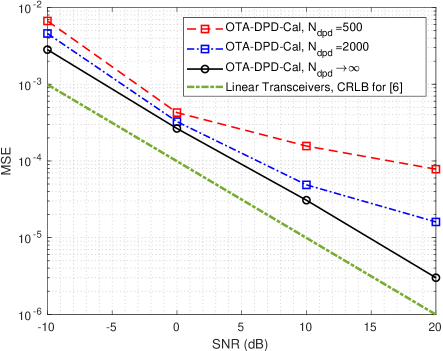
Figure 1: Average MSE of calibration matrix estimation using the proposed OTA-based DPD and Calibration.

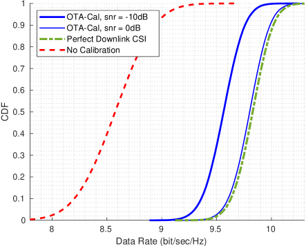
Figure 2: CDF of UEs DL Data Rate

Fig. 2 illustrates the CDF of DL data rate with our proposed method. We have generated $10^{4}$ DL channel realizations with i.i.d. Rayleigh fading channel and the DL signal power for each UE is selected to achieve an average SNR of $10$ dB at their receivers. We have selected $N_{\text{cal}}=500$ for the OTA reciprocity calibration. For comparison, we have included two extreme cases with perfect DPD as benchmarks, one with a perfect DL CSI available, and one with no calibration. To have a fair comparison with the benchmarks in terms of DPD performance, and since the results in Fig. 1 show very close MSE performance between limited-size and infinite-size OTA-DPD cases, we consider the infinite-size OTA-DPD scenario for the OTA plots. We can see that for moderate values of the reference SNR, our proposed method can significantly improve the DL data rate, and it can approach the ideal case with perfect DL CSI without requiring high-complexity iterative algorithms and dedicated hardware for performing DPD and reciprocity calibration.

V Conclusion

In this paper, we have proposed an OTA-based method for DPD and reciprocity calibration in massive MIMO systems and beyond. In particular, we considered a memory-less non-linearity model for the BS transmitters and proposed to linearize the transmitters and perform the calibration by using OTA measurements of the mutual coupling among the BS antennas. We showed that by only using the OTA data, we can effectively linearize the transmitters and perform reciprocity calibration with reduced complexity over state-of-the-art. Simulation results showed promising results in the performance of the proposed methodology, both in terms of the calibration matrix estimation error and DL data-rates when applying zero-forcing precoding after using our OTA-based DPD and calibration method.

References

- [1] E. Björnson, L. Sanguinetti, H. Wymeersch, J. Hoydis, and T. L. Marzetta, “Massive MIMO is a reality—what is next?: Five promising research directions for antenna arrays,” Digital Signal Processing, vol. 94, pp. 3–20, 2019, special Issue on Source Localization in Massive MIMO. [Online]. Available: https://www.sciencedirect.com/science/article/pii/S1051200419300776
- [2] E. G. Larsson, O. Edfors, F. Tufvesson, and T. L. Marzetta, “Massive MIMO for next generation wireless systems,” IEEE Communications Magazine, vol. 52, no. 2, pp. 186–195, 2014.
- [3] Z. Jiang, A. F. Molisch, G. Caire, and Z. Niu, “Achievable rates of FDD massive MIMO systems with spatial channel correlation,” IEEE Transactions on Wireless Communications, vol. 14, no. 5, pp. 2868–2882, 2015.
- [4] J. Flordelis, F. Rusek, F. Tufvesson, E. G. Larsson, and O. Edfors, “Massive MIMO performance—TDD versus FDD: What do measurements say?” IEEE Transactions on Wireless Communications, vol. 17, no. 4, pp. 2247–2261, 2018.
- [5] H. Wei, D. Wang, H. Zhu, J. Wang, S. Sun, and X. You, “Mutual coupling calibration for multiuser massive MIMO systems,” IEEE Transactions on Wireless Communications, vol. 15, no. 1, pp. 606–619, 2015.
- [6] J. Vieira, F. Rusek, O. Edfors, S. Malkowsky, L. Liu, and F. Tufvesson, “Reciprocity calibration for massive MIMO: Proposal, modeling, and validation,” IEEE Transactions on Wireless Communications, vol. 16, no. 5, pp. 3042–3056, 2017.
- [7] M. Jokinen, O. Kursu, N. Tervo, A. Pärssinen, and M. E. Leinonen, “Over-the-air phase calibration methods for 5G mmW antenna array transceivers,” IEEE Access, vol. 12, pp. 28 057–28 070, 2024.
- [8] D. Morgan, Z. Ma, J. Kim, M. Zierdt, and J. Pastalan, “A generalized memory polynomial model for digital predistortion of RF power amplifiers,” IEEE Transactions on Signal Processing, vol. 54, no. 10, pp. 3852–3860, 2006.
- [9] A. Sheikhi and O. Edfors, “Machine learning based digital pre-distortion in massive MIMO systems: Complexity-performance trade-offs,” in 2023 IEEE Wireless Communications and Networking Conference (WCNC), 2023, pp. 1–6.
- [10] A. Katz, J. Wood, and D. Chokola, “The evolution of PA linearization: From classic feedforward and feedback through analog and digital predistortion,” IEEE Microwave Magazine, vol. 17, no. 2, pp. 32–40, 2016.
- [11] F. Rottenberg, T. Feys, and N. Tervo, “Optimal training design for over-the-air polynomial power amplifier model estimation,” 2024. [Online]. Available: https://arxiv.org/abs/2404.12830
- [12] E. Björnson, L. Sanguinetti, and J. Hoydis, “Hardware distortion correlation has negligible impact on UL massive mimo spectral efficiency,” IEEE Transactions on Communications, vol. 67, no. 2, pp. 1085–1098, 2019.
- [13] F. Huang, J. Geng, Y. Wang, and D. Yang, “Performance analysis of antenna calibration in coordinated multi-point transmission system,” in 2010 IEEE 71st Vehicular Technology Conference, 2010, pp. 1–5.
- [14] S. M. Kay, Fundamentals of statistical signal processing: estimation theory. USA: Prentice-Hall, Inc., 1993.
- [15] C. Eun and E. Powers, “A new volterra predistorter based on the indirect learning architecture,” IEEE Transactions on Signal Processing, vol. 45, no. 1, pp. 223–227, 1997.
- [16] “Further elaboration on PA models for NR,” document 3GPP TSG-RAN WG4, R4-165901, Ericsson, Stockholm, Sweden, Aug. 2016.