Testing for changes in the error distribution in functional linear models
Abstract
We consider linear models with scalar responses and covariates from a separable Hilbert space. The aim is to detect change points in the error distribution, based on sequential residual empirical distribution functions. Expansions for those estimated functions are more challenging in models with infinite-dimensional covariates than in regression models with scalar or vector-valued covariates due to a slower rate of convergence of the parameter estimators. Yet the suggested change point test is asymptotically distribution-free and consistent for one-change point alternatives. In the latter case we also show consistency of a change point estimator.
MSC 2020 Classification: Primary 62R10 Secondary 62G10, 62G30
Keywords and Phrases: change-points, functional data analysis, regularized function estimators, regression, residual processes
1 Introduction
We consider a functional linear model with scalar response and covariates from a separable Hilbert space, e.g. . Structural changes in the distribution can appear, even when the parameters and do not change. For this reason we focus on detecting changes in the error distribution. If the errors were observable one could use the classical test (and change point estimators) based on the difference of the sequential empirical distribution functions of the first and the last error terms from a sample of observations, see Csörgö et al., (1997), Picard, (1985), Carlstein, (1988), Dümbgen, (1991), Hariz et al., (2005) and Hariz et al., (2007). In a regression model those tests have to be based on estimated residuals . Similar tests have been considered by Bai, (1994) in the context of ARMA-models, by Koul, (1996) in the context of nonlinear time series, by Ling, (1998) for nonstationary autoregressive models, and by Neumeyer and Van Keilegom, (2009) and Selk and Neumeyer, (2013) for nonparametric independent and time series regression models. Typically the asymptotic distribution is derived using asymptotic expansions of residual-based empirical distribution functions. For models with functional covariates those expansions can be problematic because inner products appear and those can have a slow rate of convergence (see Cardot et al., (2007), Shang and Cheng, (2015), and Yeon et al., (2023)). However, we show that under very simple non-restrictive assumptions those terms cancel for the suggested change point test statistic and thus the asymptotic distribution is the same as based on true (unobserved) errors.
Change point testing and estimation for functional data, and for the parameter in functional linear models have been considered in the literature, but not for the error distribution. Tests for changes in the functional mean and in the parameter function of autoregressive models are considered in chapters 6 and 14 in Horváth and Kokoszka, (2012). In Berkes et al., (2009) a CUSUM testing procedure to detect a change in the mean of functional observations is proposed. They apply projections on principal components of the data to estimate the mean. Aue et al., (2009) extend this result and introduce an estimator for the change point in this model and derive its limit distribution. Aston and Kirch, (2012) consider the same type of model with epidemic changes and dependent data. In Aue et al., (2018) structural breaks in the mean of functional observations are detected and dated without the application of dimension reduction techniques (as functional principal component analysis). Aue et al., (2014) propose a monitoring procedure to detect structural changes in functional linear models with functional response, allowing for dependence in the data, including functional autoregressive processes. They test for a change in the regression operator, which is the analogue to our , based on functional principal component analysis. A linear regression model with scalar response is considered in Horváth et al., (2023) who propose a tests for the detection of multiple change points in the regression parameter. The regressors in their model can be functional and can include lagged values of the response.
The paper is organized as follows. In Section 2 we define the test statistic and present model assumptions to obtain the asymptotically distribution-free hypothesis test. In Section 3 we discuss the assumptions on the parameter estimators and some examples. In Section 4 consistency of the test as well as of a change point estimator is considered in the context of one change point. Finite sample properties are shown in Section 5. Section 6 concludes the paper, in particular with an outlook on goodness-of-fit testing. The proofs are given in the appendix.
2 Model, test statistic and main result under the null
Let be a separable Hilbert space with inner product , corresponding norm and Borel-sigma field. Let , , be an independent sample of ()-valued random variables defined on the same probability space with probability measure . The data are modeled as functional linear model
with scalar response and -valued covariate , and with parameters , . The covariates are assumed to be iid with , and the errors are independent, centered, and independent of the covariates. Our aim is to test for change-points in the error distribution. In this section we consider the test statistic under the null hypothesis, where the errors are identically distributed.
Let and denote estimators for the parameters and . We build residuals , . The test statistic
based on the process
compares for each the empirical distribution functions
of the first and last residuals, respectively. Note that one can write
For the asymptotic distribution of the test statistic under the null hypothesis we assume the following conditions. Let denotes the distribution of .
-
(a.1)
,
-
(a.2)
Let be independent and identically distributed with cdf that is Hölder-continuous of order with Hölder-constant .
-
(a.3)
as for a class such that the function class
is -Donsker.
Remark 2.1
The assumptions are very mild and in particular less restrictive than typical assumptions for asymptotic distribution of residual-based empirical processes, even for finite-dimensional covariates. In assumption (a.1) only consistency is needed, no rates of convergence. Typically in the literature about residual-based procedures a bounded error density is assumed, see e.g. Akritas and Van Keilegom, (2001). Then (a.2) is fulfilled for , but (a.2) is less restrictive in the cases . Suitable conditions for the general assumption (a.3) are discussed in Section 3. One possibility for is to assume smoothness of which is a typical assumption. If in assumption (a.2), and is in a Sobolev-space with third derivatives, (a.2) holds for the estimator from Yuan and Cai, (2010). This estimator can also be applied for smaller in (a.2) if higher smoothness of is assumed.
Define the process as , but based on the true errors instead of residuals, i.e.
with
| (2.1) |
Further let be a completely tucked Brownian sheet, i.e. a centered Gaussian process on with covariance structure
Theorem 2.2
Under the assumptions (a.1)–(a.3),
| (2.2) |
and thus the process converges weakly to .
The proof of (2.2) in the theorem is given in the appendix. The weak convergence of is a classical result, see Bickel and Wichura, (1971) and Shorack and Wellner, (1986). With the continuous mapping theorem one obtains the asymptotic distribution of the test statistic under the null hypothesis of no change-point, which is the distribution of because is continuous. The test statistic is asymptotically distribution-free with the same limit distribution as for corresponding changepoint tests based on iid observations (not residuals). Let and be the -quantile of . Then the test that rejects the null hypothesis if has asymptotic level . Consistency is considered in Section 4.
Remark 2.3
The choice of as a Kolmogorov-Smirnov type test statistic is not mandatory. In principle, any continuous functional of the process can be considered. The most common ones, besides , are of Cramér-von-Mises type, e. g. or . The asymptotic distribution of these test statistics under the null hypothesis also follows from Theorem 2.2 and with
and thus these test statistics are asymptotically distribution-free as well. However, and contain the unknown quantity and must therefore be modified in order to be applied. This can be done by replacing the integral with the sample mean: and .
3 Discussion of assumptions and examples
To show validity of the Donsker-class assumption (a.3) there are sufficient conditions on covering numbers or bracketing numbers. We discuss some specific conditions on the class , examples for Hilbert spaces , and estimators for the parameter function that fulfill the conditions.
3.1 VC-class condition
Assumption (a.3) can be derived from a VC-function class condition formulated as follows. Assume that as for a class such that the class of maps
| (3.1) |
is a VC-subgraph class. By definition then
is a VC-class of sets. The class from (a.3) is the class of the corresponding indicator functions and (a.3) is fulfilled by Theorems 8.19 and 9.2 in Kosorok, (2008).
Example 3.1
We consider the Hilbert space with inner product and norm . For the parameter function we assume sparsity as in Lee and Park, (2012). Let be a basis of and assume for some finite, but unknown index set . Lee and Park, (2012) consider the estimator with
where is a chosen dimension-cut-off, are suitable weights based on initial estimators, and , . Further, . Under suitable assumptions, in particular , and is larger than the largest index in , Lee and Park, (2012) show in their Theorem 2 that for . Thus we can set
and obtain for . Further, the class of maps in (3.1), i.e.
is a finite dimensional vector space and thus a VC-class, see Lemma 2.6.15 in van der Vaart and Wellner, (1996). Then as discussed above validity of (a.3) follows. Furthermore, from Theorem 2 in Lee and Park, (2012) it also follows that our assumption (a.1) is fulfilled, and thus under assumption (a.2) the assertion of Theorem 2.2 holds.
3.2 Bracketing number condition
In this subsection we assume that is a separable Hilbert space of real-valued functions (or vectors with real components) and the inner product is increasing in the sense that from (pointwise for functions; componentwise for vectors) it follows that for all with . Then assumption (a.3) can be replaced by the condition in the next lemma.
Lemma 3.2
Assume (a.1), (a.2) and as for a function class such that the bracketing number fulfills for some . Here is the Hölder-order from assumption (a.2). Then assumption (a.3) holds.
The proof is given in the appendix.
Example 3.3
We consider the Hilbert space with inner product and norm . We assume for some and the Sobolev-space
where , and denotes the -th derivative of , . We consider the regularized estimators in Yuan and Cai, (2010), i.e.
for a suitable positive sequence converging to zero. Convergence rates of and its derivatives can be found in Corollaries 10 and 11 in Yuan and Cai, (2010). Under suitable assumptions one obtains for , and thus for the function class
By Corollary 4.3.38 in Giné and Nickl, (2021) and Lemma 9.21 in Kosorok, (2008) the class fulfills the bracketing number condition in Lemma 3.2 for . Thus the assumptions (a.1)–(a.3) are fulfilled if is Hölder-continuous of order . Less restrictive assumptions on , i.e. , require for this concept higher smoothness of .
4 Fixed one-change point alternative: consistency of the test and change point estimator
In this section we consider fixed alternatives with one change point at index with . We write the functional linear model as in Section 2 under the following assumption.
-
(a.2)’
Assume are iid with cdf , and are iid with cdf . Let and be Hölder-continuous of order with Hölder-constant , respectively.
Let further denote the distribution of (before the change) and denote the distribution of (after the change). For the empirical distribution functions and as in Section 2 we obtain the following asymptotic result.
Lemma 4.1
Under assumptions (a.1) and (a.2)’ and if (a.3) is valid for and , it holds that
The proof is given in the appendix. Now note that
and by Lemma 4.1 the right hand side converges in probability to the positive constant
From this it follows that tests that reject the null hypothesis of no change-point if for some (see Section 2) are consistent.
The estimator for the change point is based on the process and is defined as
Lemma 4.2
Under assumptions (a.1), (a.2)’ and if (a.3) holds for and , the change point estimator is consistent, i. e.
The proof is given in the appendix.
5 Finite sample properties
We consider the Hilbert space . For the functional observations , , are generated according to
where and for , . stands for the (continuous) uniform distribution. The functional linear model is built as
where the coefficient function is the density of the Gamma distribution. Furthermore, we assume that each is observed on a dense, equidistant grid of 300 evaluation points.
The parameter estimators are the regularized estimators described in Example 3.3 with and a data-driven tuning parameter chosen by generalized cross-validation as described in Yuan and Cai, (2010).
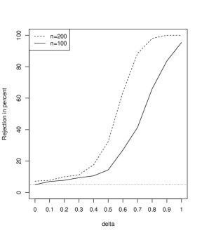
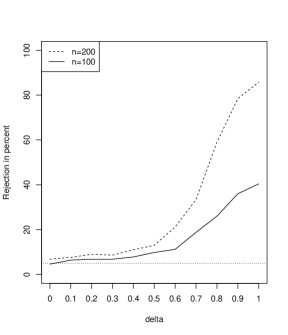
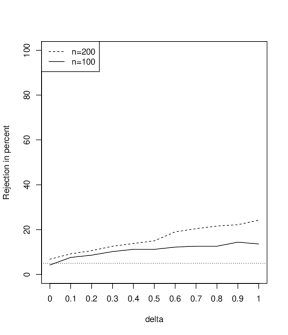
We model three similar types of change points, such that
where , , have in common that the mean remains zero and the variance remains one. In particular
-
•
is the distribution function of a random variable that is distributed with probability and distributed with probability .
-
•
is the distribution function of a random variable that is distributed with probability and distributed with probability .
-
•
is the “skew-normal”-distribution
A random variable is distributed if and has the density , where is the density and is the distribution function of the standard normal distribution (see Azzalini and Capitanio, (1999)). The expected value of such a random variable is calculated as and the variance as . This results in the parameters for the distribution after the change point, such that the the expected value of the errors remains 0 and the variance remains 1.
So represents the null hypothesis of no change point, and the difference between the distribution before and after the change point grows with in all three cases.
In Figure 1 the rejection probabilities for 500 repetitions, level 5% (critical value tabled in Picard, (1985)) and sample sizes are shown. In all three cases it can be seen that the level is approximated well and the power increases for increasing parameter as well as for increasing sample size . In the case of a change in skewness, the increase with is not as pronounced as in the other two cases. This is because the distributions for different values of become more similar as increases. The same types of changes (from to and to ) were also simulated in Selk and Neumeyer, (2013) for a real-valued nonparametric autoregression model with lag 1. The results are comparable with an even higher power in the paper at hand.
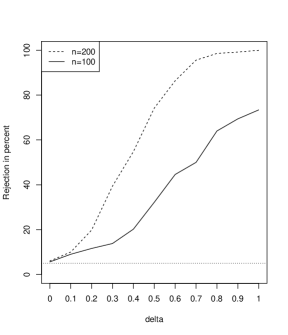
In addition, we model a more distinct change, that is
As expected for a change in the variance the power grows faster with increasing than in the other three cases, especially for small . The results are shown in Figure 2. This kind of change point was also simulated in Neumeyer and Van Keilegom, (2009) for a nonparametric regression model with one-dimensional regressor. The results are similar.
Next to the Kolmogorov-Smirnov type test with test statistic , we also applied Cramér-von-Mises type tests with test statistics and . The results are very similar and are not presented here for the sake of brevity.
6 Concluding remarks
To detect structural changes in functional linear models, we considered the classical test by Bickel and Wichura, (1971) for a change in the distribution, but based on estimated errors. We gave simple assumptions under which the asymptotic distribution of the test statistic under the null is the same as for iid data. The test as well as the corresponding change point estimators are consistent in one-change point models. The same test can be considered in more complex regression models with functional covariates, e.g. a quadratic model as in Boente and Parada, (2023) or nonparametric models, see Ferraty and Vieu, (2006). We only consider independent data, but testing for change points in the innovation distribution in times series models that include functional covariates is a very interesting topic. However, the proofs for asymptotic distributions will be more complicated. In future work we are planning to consider a time series model where and are real-valued and contains a functional part, but can also contain past values . We presume that the proofs as in Selk and Neumeyer, (2013) (for nonparametric autoregression time series with independent errors) and of section 4.2 in Neumeyer and Omelka, (2024) (for linear models with finite-dimensional covariates and beta-mixing errors) can be combined with the proofs in the paper at hand to consider change-point tests for the innovation distribution under the assumption that , , is a strictly stationary beta-mixing time series.
In the proof of Theorem 2.2 we derive an expansion for the sequential residual-based empirical distribution function,
uniformly in , where is defined in (2.1), and the term
appears from estimating the parameters (see (A.1) in the appendix). Here denotes the expectation with respect to , which has the same distribution as , but is independent of , . For change-point testing the remainder term cancels when considering the test statistic . For other testing procedures, e. g. goodness-of-fit tests for the error distribution, this typically nonnegligible term is of relevance, see Koul, (2002) and Neumeyer et al., (2006) for linear models and Akritas and Van Keilegom, (2001) for nonparametric regression. Under more restrictive assumptions one can further expand the remainder term as follows. Assume that is twice differentiable with density and bounded and further , and . Then by Taylor’s expansion one obtains
In models with intercept , where the estimator for is chosen as the remainder term is
(Here, and analogous for and .) By Cauchy-Schwarz-inequality and the central limit theorem for one obtains that the dominating part of the remainder term is . This is the same as in homoscedastic finite-dimensional linear models with intercept and nonparametric regression models. Note that and are identifiable if the kernel of the covariance operator of the covariate is . But often functional linear models without intercept are considered in the literature. So in our model assume . Then the remainder term is
and for fixed typically has a slower rate than , see Cardot et al., (2007), Shang and Cheng, (2015), Yeon et al., (2023). If one assumes , then this problematic term cancels (similar as e.g. for centered ARMA-processes, see Bai, (1994)), but otherwise will dominate the asymptotic distribution of the process . For our change-point test this dominating term vanishes. The same holds when estimating the conditional copula of the response in multidimensional functional linear models, given the covariate, see Theorem 5 in Neumeyer and Omelka, (2024). But e.g. for goodness-of-fit testing the remainder term would be of relevance. We consider goodness-of-fit tests for the error distribution in the different cases explained above in future work. With the derived expansion for residual empirical distribution functions one can also develop other tests for the error distribution as e.g. for symmetry, or equality of error distributions in different models, see e.g. Pierce and Kopecky, (1979), Neumeyer et al., (2005), Pardo Fernandez, (2007), among many others, in the cases of regression models with finite-dimensional covariates.
Appendix A Proofs
For ease of notation let be some generic random variable with the same distribution as under the null, but independent from the sample , . Let denote the distribution of . Further let denote the expectation with respect to , which in the context below is the conditional expectation given , .
The proofs of Theorem 2.2 and Lemma 3.2 are similar as a part of the proof of Theorem 5 in Neumeyer and Omelka, (2024), but under less restrictive assumptions.
A.1 Proof of Theorem 2.2
From the Donsker-property in assumption (a.3) and Corollary 9.31 in Kosorok, (2008) it follows that
is also -Donsker. From Theorem 2.12.1 in van der Vaart and Wellner, (1996) it follows that also the centered sequential process
indexed in , , , , converges weakly to a centered Gaussian process. Thus the process is asymptotically stochastic equicontinuous with respect to the semi-metric
see van der Vaart and Wellner, (1996), problem 2, p. 93, and section 2.12. In particular we need
by Cauchy-Schwarz and Jensen’s inequality. Now setting and we obtain convergence to zero in probability by assumption (a.1). Thus from asymptotic stochastic equicontinuity of the process , and we obtain that
which means that
uniformly in , where was defined in (2.1) and is based on the true errors. In particular for we have
uniformly in . From those expansions we obtain
| (A.2) | |||||
uniformly in .
A.2 Proof of Lemma 3.2
Let and let
be brackets for of -length (see assumption (a.3)). Now for the indicator function is contained in the bracket
for each . Further the above bracket has -length
by assumption (a.2), Cauchy-Schwarz and Jensen’s inequality. Similar to the proof of Lemma 1 in Akritas and Van Keilegom, (2001) one obtains an upper bound for the -bracketing number of the class . Thus is -Donsker by the bracketing integral condition in Theorem 19.5 of van der Vaart, (1998).
A.3 Proof of Lemma 4.1
To show the assertion for we use the arguments as in the proof of Theorem 2.2 for the process , but based on the iid sample before the change. Then as in the proof of Theorem 2.2 asymptotic stochastic equicontinuity of the process holds and thus
Here, and depend on the whole sample and assumption (a.1) is used. Thus as in equation (A.1) we obtain
uniformly in . By the classical Glivenko-Cantelli result converges uniformly almost surely to . By assumptions (a.1), (a.2)’ and the remainder term is and the assertion for follows.
The assertion for can be shown analogously.
A.4 Proof of Lemma 4.2
First note that
Further it holds
since we have
| (A.3) | ||||
| (A.4) | ||||
Here we have used Lemma 4.1 for the term (A.4). Further is defined as based on the iid-sample , but where the residuals are built with , based on the whole sample. With the same argument as in the proof of Theorem 2.2 it holds that
Analogously one can show that .
Thus, it holds uniformly in
The assertion then follows by Theorem 2.12 in Kosorok, (2008) as is well-separated maximum of .
References
- Akritas and Van Keilegom, (2001) Akritas, M. G. and Van Keilegom, I. (2001). Non-parametric estimation of the residual distribution. Scandinavian Journal of Statistics, 28(3):549–567.
- Aston and Kirch, (2012) Aston, J. A. D. and Kirch, C. (2012). Detecting and estimating changes in dependent functional data. Journal of Multivariate Analysis, 109:204–220.
- Aue et al., (2009) Aue, A., Gabrys, R., Horváth, L., and Kokoszka, P. (2009). Estimation of a change-point in the mean function of functional data. Journal of Multivariate Analysis, 100(10):2254–2269.
- Aue et al., (2014) Aue, A., Hörmann, S., Horváth, L., and Hušková, M. (2014). Dependent functional linear models with applications to monitoring structural change. Statistica Sinica, 24:1043–1073.
- Aue et al., (2018) Aue, A., Rice, G., and Sönmez, O. (2018). Detecting and dating structural breaks in functional data without dimension reduction. Journal of the Royal Statistical Society Series B: Statistical Methodology, 80(3):509–529.
- Azzalini and Capitanio, (1999) Azzalini, A. and Capitanio, A. (1999). Statistical applications of the multivariate skew-normal distribution. Journal of the Royal Statistical Society Series B: Statistical Methodology, 61:579–602.
- Bai, (1994) Bai, J. (1994). Weak convergence of the sequential empirical processes of residuals in ARMA models. The Annals of Statistics, 22:2051–2061.
- Berkes et al., (2009) Berkes, I., Gabrys, R., Horváth, L., and Kokoszka, P. (2009). Detecting changes in the mean of functional observations. Journal of the Royal Statistical Society Series B: Statistical Methodology, 71(5):927–946.
- Bickel and Wichura, (1971) Bickel, P. J. and Wichura, M. J. (1971). Convergence criteria for multiparameter stochastic processes and some applications. The Annals of Mathematical Statistics, 42:1656–1670.
- Boente and Parada, (2023) Boente, G. and Parada, D. (2023). Robust estimation for functional quadratic regression models. Computational Statistics & Data Analysis, 187.
- Cardot et al., (2007) Cardot, H., Mas, A., and Sarda, P. (2007). CLT in functional linear regression models. Probability Theory and Related Fields, 138:325–361.
- Carlstein, (1988) Carlstein, E. (1988). Nonparametric change-point estimation. The Annals of Statistics, 16(1):188–197.
- Csörgö et al., (1997) Csörgö, M., Horváth, L., and Szyszkowicz, B. (1997). Integral tests for suprema of kiefer processes with application. Statistics & Decisions, 15:365–377.
- Dümbgen, (1991) Dümbgen, L. (1991). The asymptotic behavior of some nonparametric change-point estimators. The Annals of Statistics, 19(3):1471–1495.
- Ferraty and Vieu, (2006) Ferraty, F. and Vieu, P. (2006). Nonparametric Functional Data Analysis. Springer Series in Statistics. Springer, New York.
- Giné and Nickl, (2021) Giné, E. and Nickl, R. (2021). Mathematical Foundations of Infinite-Dimensional Statistical Models. Cambridge Series in Statistical and Probabilistic Mathematics. Cambridge University Press.
- Hariz et al., (2005) Hariz, S. B., Wylie, J. J., and Zhang, Q. (2005). Nonparametric change-point estimation for dependent sequences. Comptes Rendus Mathematique, 341(10):627–630.
- Hariz et al., (2007) Hariz, S. B., Wylie, J. J., and Zhang, Q. (2007). Optimal rate of convergence for nonparametric change-point estimators for nonstationary sequences. The Annals of Statistics, 35(4):1802–1826.
- Horváth and Kokoszka, (2012) Horváth, L. and Kokoszka, P. (2012). Inference for Functional Data with Applications. Springer Series in Statistics. Springer New York.
- Horváth et al., (2023) Horváth, L., Kokoszka, P., and Lu, S. (2023). Testing for parameter changes in high dimensional regression with autoregressive dependence. ArXiv.
- Kosorok, (2008) Kosorok, M. R. (2008). Introduction to empirical processes and semiparametric inference. Springer New York.
- Koul, (1996) Koul, H. L. (1996). Asymptotics of some estimators and sequential residual empiricals in nonlinear time series. The Annals of Statistics, 24:380–404.
- Koul, (2002) Koul, H. L. (2002). Weighted Empirical Processes in Dynamic Nonlinear Models. Lecture Notes in Statistics. Springer New York.
- Lee and Park, (2012) Lee, E. R. and Park, B. U. (2012). Sparse estimation in functional linear regression. Journal of Multivariate Analysis, 105(1):1–17.
- Ling, (1998) Ling, S. (1998). Weak convergence of the sequential empirical processes of residuals in nonstationary autoregressive models. The Annals of Statistics, 26:741–754.
- Neumeyer et al., (2005) Neumeyer, N., Dette, H., and Nagel, E.-R. (2005). A note on testing symmetry of the error distribution in linear regression models. Journal of Nonparametric Statistics, 17(6):697–715.
- Neumeyer et al., (2006) Neumeyer, N., Dette, H., and Nagel, E.-R. (2006). Bootstrap tests for the error distribution in linear and nonparametric regression models. Australian & New Zealand Journal of Statistics, 48(2):129–156.
- Neumeyer and Omelka, (2024) Neumeyer, N. and Omelka, M. (2024). Generalized Hadamard differentiability of the copula mapping and its applications. Bernoulli, to appear.
- Neumeyer and Van Keilegom, (2009) Neumeyer, N. and Van Keilegom, I. (2009). Change-point tests for the error distribution in non-parametric regression. Scandinavian Journal of Statistics, 36(3):518–541.
- Pardo Fernandez, (2007) Pardo Fernandez, J. C. (2007). Comparison of error distributions in nonparametric regression. Statistics & Probability Letters, 77:350–356.
- Picard, (1985) Picard, D. (1985). Testing and estimating change-points in time series. Advanced Applied Probability, 17:841–867.
- Pierce and Kopecky, (1979) Pierce, D. A. and Kopecky, K. J. (1979). Testing goodness of fit for the distribution of errors in regression models. Biometrika, 66(1):1–5.
- Selk and Neumeyer, (2013) Selk, L. and Neumeyer, N. (2013). Testing for a change of the innovation distribution in nonparametric autoregression: The sequential empirical process approach. Scandinavian Journal of Statistics, 40(4):770–788.
- Shang and Cheng, (2015) Shang, Z. and Cheng, G. (2015). Nonparametric inference in generalized functional linear models. The Annals of Statistics, 43(4):1742–1773.
- Shorack and Wellner, (1986) Shorack, G. R. and Wellner, J. A. (1986). Empirical processes with applications to statistics. John Wiley & Sons.
- van der Vaart, (1998) van der Vaart, A. (1998). Asymptotic Statistic. Cambridge Series in Statistical and Probabilistic Mathematics. Cambridge University Press.
- van der Vaart and Wellner, (1996) van der Vaart, A. and Wellner, J. A. (1996). Weak convergence and empirical processes. Springer New York.
- Yeon et al., (2023) Yeon, H., Dai, X., and Nordman, D. J. (2023). Bootstrap inference in functional linear regression models with scalar response. Bernoulli, 29(4):2599–2626.
- Yuan and Cai, (2010) Yuan, M. and Cai, T. (2010). A reproducing kernel Hilbert space approach to functional linear regression. The Annals of Statistics, 38(6):3412–3444.