Improve the Fitting Accuracy of Deep Learning for the Nonlinear Schrödinger Equation Using Linear Feature Decoupling Method

Abstract

We utilize the Feature Decoupling Distributed (FDD) method to enhance the capability of deep learning to fit the Nonlinear Schrödinger Equation (NLSE), significantly reducing the NLSE loss compared to non decoupling model.

I Introduction

The Nonlinear Schrödinger Equation (NLSE) describes propagation of optical pulses through optical fiber channel, which is the cornerstone for studying nonlinear optics and optical fiber communication[1][2]. The NLSE is non-analytical when both linearity and nonlinearity are considered. Traditional method to solve NLSE is based on Split-Step Fourier method (SSFM)[3], which is a numerical method and needs large iteration, leading to high computational complexity and making it challenging to meet practical engineering application[9].

Recently, deep learning (DL) has emerged as a accurate and efficient approach for solving NLSE and modeling optical fiber channel, owing to its their strong nonlinear fitting capabilities and efficiency in parallel computation. Neural networks, such as BiLSTM, CGAN and Transformer have succeed in modeling optical fiber channel in signal- and multi-channel WDM systems[6][7][10]. Physics informed neural networks has achieved modeling of fiber channels or optical pulses under specific boundary conditions[4][5].

However, most existing DL-based schemes utilize pure-data driven or incorporate physical prior knowledge in the loss function. NNs need to learn all linear and nonlinear coupled characteristic from whole NLSE, which face accuracy degrade in more complex scenarios. Meanwhile, NNs may have learned only the features of the training data, not the mappings that satisfy the NLSE equation.

In this paper, we utilize a feature decoupling distributed (FDD) method to fit NLSE in optical fiber communication.This method decouple the linear features by combining prior physical models. By embedding parameters and differentiating signal waves, the NLSE loss is assessed during training, allowing for further performance analysis. The FDD method demonstrates a threefold reduction in the predicted waveform Normalized Mean Square Error (NMSE) during training scenarios compared to the non-decoupled method. Furthermore, in non-training scenarios, the waveform NMSE is reduced by more than tenfold. For transmission distances ranging from 10-100 km, the NMSE accuracy of the FDD model remains below , with a two-order magnitude reduction in NLSE loss. These results demonstrates that the FDD model achieves superior accuracy over the non-decoupling model and adapts effectively across a broader range of boundary conditions.

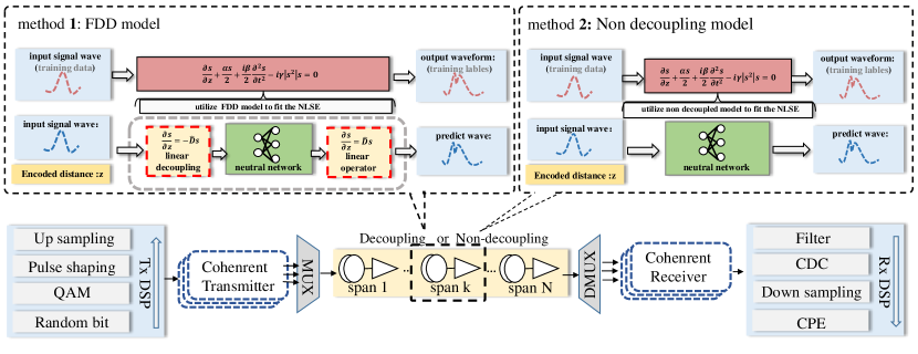
Figure 1: Two methods for fitting the NLSE.

II Principle

II-A The Nonlinear Schrödinger Equation (NLSE)

The Nonlinear Schrödinger Equation (NLSE) is a type of Partial Differential Equations (PDEs), it describes the dispersion, nonlinear effects, and gain-loss experienced by the optical pulse as it travels through the fiber. Considering the Polarization Mode Dispersion (PMD) effect, its general form is:

$$\begin{split}\frac{\partial s}{\partial z}+\frac{\alpha s}{2}+\frac{i\beta}{2}\frac{\partial^{2}s}{\partial t^{2}}-\frac{8}{9}i\gamma|s|^{2}s=0,\end{split}$$ (1)

where $s$$=$ $s(z,t)$ represents the optical field envelope, $z$ is the propagation distance, $t$ is time, $\beta_{2}$ is the dispersion coefficient, $\alpha$ is the attenuation coefficient, and $\gamma$ is the nonlinear coefficient. Traditional methods for solving the NLSE use numerical simulations. The most commonly used method for solving equation (1) is the Split-Step Fourier Method (SSFM) [1]. NLSE can be written in the form of linear and nonlinear operators for signal operations, as shown in equatuin(2),

$$\begin{split}\frac{\partial S(z,t)}{\partial z}=\left(\hat{D}+\hat{N}[S(z,t)]\right)S(z,t),\end{split}$$ (2)

where $\hat{D}$ is the linear component, which denotes the effects of attenuation and CD, and $\hat{N}$ is the nonlinear component, $S$ denotes the optical field complex envelope, $z$ represents the distance, and $t$ is the time, so the SSFM treats the fiber channel propagation system as an alternating iteration of nonlinear and linear steps.

II-B Principle of utilizing FDD model to fit NLSE

In the method of utilizing purely data-driven neural networks to simulate the NLSE, the neural network directly learns both the linear and nonlinear aspects of the entire NLSE system, as shown in Figure 1. From (2), it can be seen that the NLSE equation includes both linear and nonlinear operators. Therefore, to mitigate the linear effects after the entire transmission and introduce physical formula modeling, we adopt Feature Decoupling Distribution (FDD) modeling in the neural network part. This approach reduces the difficulty of fitting the neural network, however, the neural network itself no longer conforms to the NLSE. To allow the neural network to fully fit the NLSE, a linear system modeled using physical formulas is cascaded after the neural network. The linear syetem corresponds to the inverse process of dispersion compensation and distance attenuation compensation before the neural network, which can be regarded as a linear operator, as shown in Equation (3),

$$\frac{\partial s}{\partial z}+\frac{\alpha s}{2}+\frac{i\beta}{2}\frac{\partial^{2}s}{\partial t^{2}}=0,$$ (3)

where $s$$=$ $s(z,t)$ represents the optical field envelope, $z$ is the propagation distance, $t$ is time, $\beta_{2}$ is the dispersion coefficient, $\alpha$ is the attenuation coefficient.The frequency domain analytical solution is given in Equation (4),

$$S(z+L_{\text{span}},\omega)=S(z,\omega)\exp\left(-\frac{i\beta_{2}}{2}\omega^{2}L_{\text{span}}\right),$$ (4)

where $S(z,w)$ is the Fourier transform of $s(z,t)$ , and $L_{\text{span}}$ is the transmission distance for one span.The equivalent system formed by cascading the neural network and the linear system can fit the complete NLSE system.To derive the output waveform with respect to the distance parameter $z$ and enhance the model’s generalization over distances, we have implemented an encoded input method for $z$ at the input end[8]. The chosen neural network is Bidirectional Long Short-Term Memory (BiLSTM), known for its capability to capture and learn the dependencies in the input signals[7].

To obtain NLSE loss for non decoupling and FDD systems, we need to calculate the derivatives of the output signal with respect to the distance $z$ and time $t$ for the neural network. We introduce a parameter $z$ that controls the distance encoded by the neural network at the input end[8]. We utilize the feature of neural networks that can back propagate and take derivatives, we obtain the derivative of the output predicted waveform with respect to $z$. Due to the fact that our neural network is used for time-domain waveform simulation modeling without inputting the time parameter t at the input, the derivative of time $t$ is obtained by directly taking the second-order derivative of the output waveform in time-domain. The output time-domain waveform is transformed to the frequency domain using the Fourier transform, and multiplied by $iw$ squared in the frequency domain to obtain the second-order derivative of the system with respect to time, as shown in Equation (5).

$$\mathcal{F}\left\{\frac{\partial^{2}s}{\partial t^{2}}\right\}=(i\omega)^{2}\mathcal{F}\{s(z,t)\},$$ (5)

where $\mathcal{F}$ represents Fourier transform and $i$ represents imaginary unit. Since the simulation system we are using is a dual polarization system, we need to consider the Polarization Mode Dispersion (PMD) effect, by deriving the NLSE, we can obtain the fiber channel formula that takes into account the PMD effect, namely the Manakov PMD equation, we substitute the time and distance derivatives of the signal and the obtained signal into equation (6) which shown as:

$$\ NLSEloss=\frac{\partial s}{\partial z}+\frac{\alpha s}{2}+\frac{i\beta}{2}\frac{\partial^{2}s}{\partial t^{2}}-\frac{8}{9}i\gamma|s|^{2}s,$$ (6)

to obtain the NLSE loss of the system, where $s$ represents a signal containing two orthogonal polarization modes.

III Simulation and results discussion

III-A Simulation and training setup

To collect training data and analyze the performance of channel modeling, we simulated a dual-polarization coherent WDM optical transmission system, as shown in Figure 1. The symbol rate is 30 Gbaud per channel, and the channel spacing is 50 GHz. The modulation format is dual-polarization 16 QAM, with 5 channels, and each channel has a transmit power of 5 dBm. The transmitter uses a root-raised cosine (RRC) filter with a roll-off factor of 0.1 for pulse shaping. To simulate the time-domain waveform, the channel employs 4x oversampling and uses the SSFM algorithm for simulation, as shown in Figure 1 .To enable the neural network to learn the characteristics of signal waveforms that change with different times and distances, optical signal data was collected at transmission distances of 10 km, 20 km, 30 km, 50 km, and 70 km. After passing through the backward dispersion system, the complex signals of the two polarization channels are arranged into a one-dimensional vector. The transmission distance parameter $z$ is also encoded by a linear layer and input into a neural network.

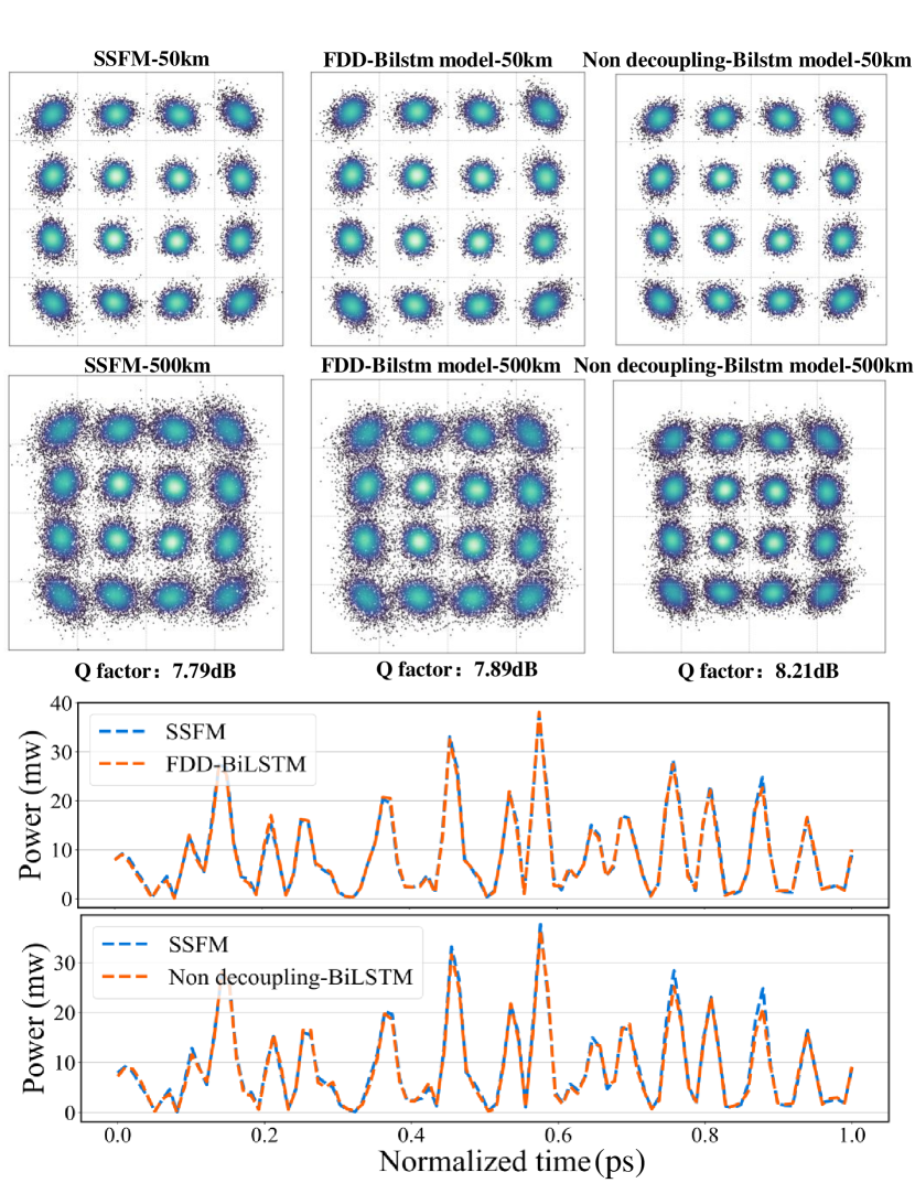
Figure 2: The model accuracy of FDD model and non decoupling model.

III-B Accuracy of non decoupling model and FDD model

We compared the waveforms, constellations, Q-factors, and NMSE accuracy of the FDD model and the non decoupling model at different transmission distances to verify that the FDD model has higher waveform prediction accuracy. After DSP processing of the output waveform, as shown in Figure 2, the data points in the FDD model constellations have a rotation degree that is basically consistent with SSFM. Clearly, compared to the non decoupling model, the constellations of the FDD model exhibits consistent rotation with the constellations obtained from numerical methods, indicating that linear decoupling helps the neural network better learn the nonlinear parts of the NLSE equation. Additionally, the time-domain waveform diagram also shows that the waveforms closely match the theoretical values, which demonstrates that FDD model has higher waveform prediction accuracy.

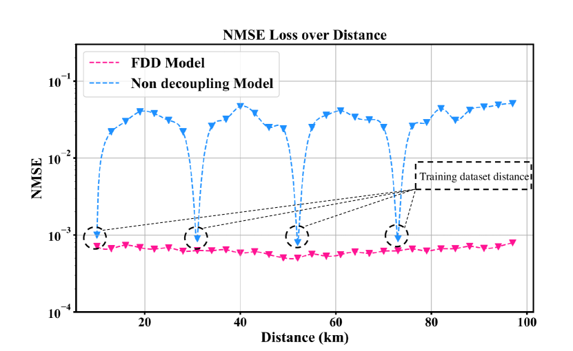
Figure 3: NMSE of non decoupling systems and FDD model.

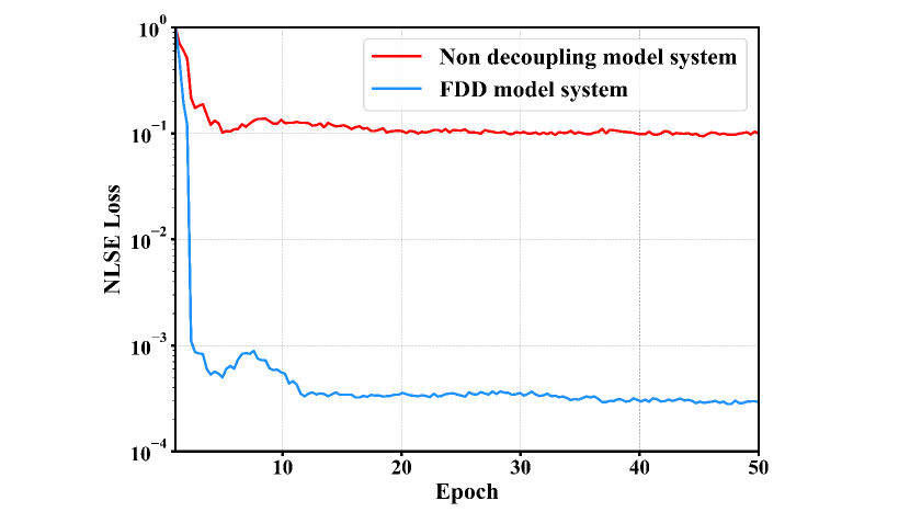
Figure 4: NLSE loss training curve of non decoupling model and FDD model.

To verify that the FDD model has better generalization to distance and obtains a mapping that adapts in a wider range of boundary conditions compared to the non decoupling model, we plotted the NMSE accuracy comparison of the predicted output waveforms of the two models with different distance parameters as input. It can be seen that the waveform error accuracy of the FDD model is 1-2 orders of magnitude lower than that of the non decoupling model. From the figure, it can be seen that although both models adopted the training model with distance parameter $z$ as input, the non decoupled model only has high accuracy in the distance of the training dataset, at untrained distance points, the accuracy of waveform NMSE still significantly decreases, indicating that it only learned some local optima. In contrast, the FDD model maintained high prediction accuracy for the optical signal waveform transmission over distances of 10-100 km, this indicates that the FDD model has higher accuracy in distance generalization and can obtain a mapping that adapts in a wider range of boundary conditions.

III-C NLSE loss of FDD model system and non decoupling model system

To further demonstrate that the FDD model fits the NLSE equation better, we also presented the changes in NLSE loss during the training process for both the non decoupling model and the FDD model. The NLSE loss is calculated by equation (6) and the average NLSE loss of 1000 signals is taken. The NLSE loss of the non decoupling model is around the order of $10^{-2}$, showing some decline only at the beginning of the training. This indicates that the non decoupling model clearly failing to learn the equation varying with parameters $z$ and $t$, but merely fitting to specific data features. In contrast, as the number of epochs increases, the overall NLSE loss continues to gradually decrease to a lower level, with the signal amplitude around the order of and the average single-symbol NLSE loss around the order of $10^{-4}$, as shown in Figure 4. In FDD model, the linear effects of the FDD model system are modeled by equations which incorporates prior physical knowledge of the linear part into the system, thus, at the beginning of the training, the linear part of the NLSE equation is already correct, allowing the neural network to focus on optimizing the nonlinear part. The lower NLSE loss explains why the FDD model has stronger distance generalization capabilities and can obtain a mapping that adapts in a wider range of boundary conditions.

IV Conclusion

To simplify the difficulty of fitting the NLSE equation and improve the accuracy of neural networks in fitting the NLSE equation, we applied the Feature Decoupling Distribution (FDD) method in neural networks for NLSE modeling, we analyzed and calculated the NLSE loss of both the FDD model and the non decoupling model and compared their distance generalization accuracy. Since the FDD model incorporates prior physical knowledge of the linear part of the NLSE into the system, the FDD model can better fit and approximate the original NLSE. We found that the FDD model’s accuracy and distance generalization are higher than that of the non decoupling model. Additionally, the NLSE loss of the FDD model is significantly lower than that of the non decoupling system which indicates that FDD model can obtain a mapping that adapts in a wider range of boundary conditions. We believe that this method of utilizing linear feature decoupling can also be applied to neural networks that fit physical processes controlled by other Partial Differential Equations(PDEs), enabling these networks to better fit the PDEs.

References

- [1] Agrawal G P. Nonlinear fiber optics[M]//Nonlinear Science at the Dawn of the 21st Century. Berlin, Heidelberg: Springer Berlin Heidelberg, 2000: 195-211.
- [2] Salmela L, Tsipinakis N, Foi A, et al. Predicting ultrafast nonlinear dynamics in fibre optics with a recurrent neural network[J]. Nature machine intelligence, 2021, 3(4): 344-354.
- [3] N. A. Kudryashov, ”A generalized model for description of propagation pulses in optical fiber,” Optik. 189, 42-52 (2019), Doi: 10.1016/j.ijleo.2019.05.069.
- [4] Raissi M, Perdikaris P, Karniadakis G E. Physics-informed neural networks: A deep learning framework for solving forward and inverse problems involving nonlinear partial differential equations[J]. Journal of Computational physics, 2019, 378: 686-707.
- [5] Song Y, Wang D, Fan Q, et al. Physics-informed neural operator for fast and scalable optical fiber channel modelling in multi-span transmission[C]//2022 European Conference on Optical Communication (ECOC). IEEE, 2022: 1-4.
- [6] Jiang X, Wang D, Fan Q, et al. Solving the nonlinear Schrödinger equation in optical fibers using physics-informed neural network[C]//Optical fiber communication conference. Optica Publishing Group, 2021: M3H. 8.
- [7] Yang H, Niu Z, Zhao H, et al. Fast and accurate waveform modeling of long-haul multi-channel optical fiber transmission using a hybrid model-data driven scheme[J]. Journal of Lightwave Technology, 2022, 40(14): 4571-4580.
- [8] Zeng C, Niu Z, Yang H, et al. Enhancing Generalization in Neural Channel Model for Optical Fiber WDM Transmission through Learned Encoding of System Parameters[C]//2024 Optical Fiber Communications Conference and Exhibition (OFC). IEEE, 2024: 1-3.
- [9] Serena P, Lasagni C, Musetti S, et al. On numerical simulations of ultra-wideband long-haul optical communication systems[J]. Journal of Lightwave Technology, 2019, 38(5): 1019-1031.
- [10] Shi M, Yang H, Niu Z, et al. Accurate and Efficient Optical Fiber WDM Transmission Modeling Using the Encoder-Only Transformer with Feature Decoupling Distributed Method[C]//2023 Asia Communications and Photonics Conference/2023 International Photonics and Optoelectronics Meetings (ACP/POEM). IEEE, 2023: 1-5.