Butterfly factorization with error guarantees

Abstract

In this paper, we investigate the butterfly factorization problem, i.e., the problem of approximating a matrix by a product of sparse and structured factors. We propose a new formal mathematical description of such factors, that encompasses many different variations of butterfly factorization with different choices of the prescribed sparsity patterns. Among these supports, we identify those that ensure that the factorization problem admits an optimum, thanks to a new property called “chainability”. For those supports we propose a new butterfly algorithm that yields an approximate solution to the butterfly factorization problem and that is supported by stronger theoretical guarantees than existing factorization methods. Specifically, we show that the ratio of the approximation error by the minimum value is bounded by a constant, independent of the target matrix.

1 Introduction

Algorithms for the rapid evaluation of linear operators are important tools in many domains like scientific computing, signal processing, and machine learning. In such applications, where a very large number of parameters is involved, the direct computation of the matrix-vector multiplication hardly scales due to its quadratic complexity in the matrix size. Many existing works therefore rely on analytical or algebraic assumptions on the considered matrix to approximate the evaluation of matrix-vector multiplication with a subquadratic complexity. Examples of such structures include low-rank matrices, hierarchical matrices [15], fast multipole methods [11], etc.

Among these different structures, previous work has identified another class of matrices that can be compressed for accelerating matrix multiplication. It is the class of so-called butterfly matrices [31, 33, 2], and includes many matrices appearing in scientific computing problems, like kernel matrices associated with special function transforms [33, 42] or Fourier integral operators [2, 7, 24]. Such matrices satisfy a certain low-rank property, named the complementary low-rank property [23]: it has been shown that if specific submatrices of a target matrix $\mathbf{A}$ of size $n\times n$ are numerically low-rank, then $\mathbf{A}$ can be compressed by successive hierarchical low-rank approximations of these submatrices, and that as a result it can be approximated by a sparse factorization

$$\hat{\mathbf{A}}={\mathbf{X}}_{1}\ldots{\mathbf{X}}_{L}$$

with $L=\mathcal{O}(\log n)$ factors $\mathbf{X}_{\ell}$ having at most $\mathcal{O}(n)$ nonzero entries for each $\ell\in\llbracket L\rrbracket:=\{1,\ldots,L\}$. This sparse factorization, called in general butterfly factorization, would then yield a fast algorithm for the approximate evaluation of the matrix-vector multiplication by $\mathbf{A}$, in $\mathcal{O}(n\log n)$ complexity.

An alternative definition of the butterfly factorization refers to a sparse matrix factorization with specific constraints on the sparse factors. According to [5, 6, 20, 44, 4, 27], a matrix $\mathbf{A}$ admits a certain butterfly factorization if, up to some row and column permutations, it can be factorized into a certain number of factors ${\mathbf{X}}_{1},\ldots,{\mathbf{X}}_{L}$ for a prescribed number $L\geq 2$, such that each factor ${\mathbf{X}}_{\ell}$ for $\ell\in\llbracket L\rrbracket$ satisfies a so-called fixed-support constraint, i.e., the support of ${\mathbf{X}}_{\ell}$, denoted $\mathtt{supp}({\mathbf{X}}_{\ell})$, is included in the support of a prescribed binary matrix ${\mathbf{S}}_{\ell}$. The different existing butterfly factorizations only vary by their number of factors $L$, and their choice of binary matrices ${\mathbf{S}}_{1},\ldots,{\mathbf{S}}_{L}$. Let us give some examples of such factorizations.

1. Square dyadic butterfly factorization [5, 6, 20, 44]. It is defined for matrices of size $n\times n$ where $n$ is a power of two. The number of factors is $L:=\log_{2}n$. For $\ell\in\llbracket L\rrbracket$, the factor ${\mathbf{X}}_{\ell}$ is of size $n\times n$, and satisfies the support constraint $\mathtt{supp}({\mathbf{X}}_{\ell})\subseteq\mathtt{supp}({\mathbf{S}}_{\ell})$, where

   $$\forall\ell\in\llbracket L\rrbracket,\quad{\mathbf{S}}_{\ell}:=\mathbf{I}_{2^{\ell-1}}\otimes\mathbf{1}_{2\times 2}\otimes\mathbf{I}_{n/2^{\ell}}.$$

   Here, $\mathbf{I}_{n}$ denotes the identity matrix of size $n$, $\mathbf{1}_{p\times q}$ denotes the matrix of size $p\times q$ full of ones, and $\otimes$ denotes the Kronecker product. This butterfly factorization appears in many structured linear maps commonly used in machine learning and signal processing, like the Hadamard matrix, or the discrete Fourier transform (DFT) matrix (up to the bit-reversal permutation of column indices). Other structured matrices like circulant matrix, Toeplitz matrix or Fastfood transform [41] can be written as a product of matrices admitting such a butterfly factorization, up to matrix transposition [6]. This factorization is also used to design structured random orthogonal matrices [36], and for quadrature rules on the hypersphere [32].

2. Monarch factorization [4]. A Monarch factorization parameterized by two integers $p$, $q$ decomposes a matrix $\mathbf{A}$ of size $m\times n$ into $L:=2$ factors ${\mathbf{X}}_{1}$, ${\mathbf{X}}_{2}$ such that $\mathtt{supp}({\mathbf{X}}_{\ell})\subseteq\mathtt{supp}({\mathbf{S}}_{\ell})$ for $\ell=1,2$ where

   $${\mathbf{S}}_{1}:=\mathbf{1}_{p\times q}\otimes\mathbf{I}_{\frac{m}{p}},\quad{\mathbf{S}}_{2}:=\mathbf{I}_{q}\otimes\mathbf{1}_{\frac{m}{p}\times\frac{n}{q}}.$$

   Here, we assume that $p$, $q$ divides $m$, $n$ respectively. The DFT matrix of size $n\times n$ admits such a factorization for $p=q$, up to a column permutation. Indeed, according to the Cooley-Tukey algorithm, computing the discrete Fourier transform of size $n$ is equivalent to performing $p$ discrete Fourier transforms of size $n/p$ first, and then $n/p$ discrete Fourier transforms of size $p$, see, e.g., equations (14) and (21) in [9].

3. Deformable butterfly factorization [27]. Previous conventional butterfly factorizations can be generalized as follows. Given an integer $L\geq 2$, a matrix $\mathbf{A}$ admits a deformable butterfly factorization parameterized by a list of tuples $(p_{\ell},q_{\ell},r_{\ell},s_{\ell},t_{\ell})_{\ell=1}^{L}$ if $\mathbf{A}={\mathbf{X}}_{1}\ldots{\mathbf{X}}_{L}$ where each factor ${\mathbf{X}}_{\ell}$ for $\ell\in\llbracket L\rrbracket$ is of size $p_{\ell}\times q_{\ell}$ and has a support included in $\mathtt{supp}(\mathbf{S}_{\ell})$, defined as:

   $$\forall\ell\in\llbracket L\rrbracket,\quad\mathbf{S}_{\ell}:=\mathbf{I}_{\frac{p_{\ell}}{r_{\ell}t_{\ell}}}\otimes\mathbf{1}_{r_{\ell}\times s_{\ell}}\otimes\mathbf{I}_{t_{\ell}}.$$

   Here, it is assumed that $\frac{p_{\ell}}{r_{\ell}t_{\ell}}=\frac{q_{\ell}}{s_{\ell}t_{\ell}}$ is an integer, for each $\ell\in\llbracket L\rrbracket$.

In all these examples the fixed-support constraint on each factor $\mathbf{X}$ takes the form $\mathtt{supp}(\mathbf{X})\subseteq\mathtt{supp}(\mathbf{I}_{a}\otimes\mathbf{1}_{b\times c}\otimes\mathbf{I}_{d})$ for some integer parameters $(a,b,c,d)$. Figure 1 illustrates the sparsity pattern $\mathbf{S}_{\boldsymbol{\pi}}\coloneqq\mathbf{I}_{a}\otimes\mathbf{1}_{b\times c}\otimes\mathbf{I}_{d}$ of a factor associated with the tuple ${\boldsymbol{\pi}}=(a,b,c,d)$, that we call a pattern. One of the main benefits of choosing such fixed-support constraints instead of an arbitrary sparse support is its block structure that enables efficient implementation on specific hardware like Intelligence Processing Unit (IPU) [39] or GPU [5, 4, 13], with practical speed-up for matrix multiplication.

Such butterfly factorizations have been used in some machine learning applications. In line with recent works [5, 6, 4, 27], the parameterization (2) can be used to construct a generic representation for structured matrices that is not only expressive, but also differentiable and thus compatible with machine learning pipelines involving gradient-based optimization of parameters given training samples. The expected benefits then range from a more compressed storage and better generalization properties (thanks to the reduced number of parameters) to possibly faster implementations. For instance:

• The square dyadic butterfly factorization was used to replace hand-crafted structures in speech processing models or channel shuffling in certain convolutional neural networks, or to learn a latent permutation [6].

• The Monarch parameterization [4] of certain weight matrices in transformers for vision or language tasks led to speed-ups of training and inference time.

• Certain choices of deformable butterfly parameterizations [27] of kernel weights in convolutional layers, for vision tasks, led to similar performance as the original convolutional neural network with fewer parameters.

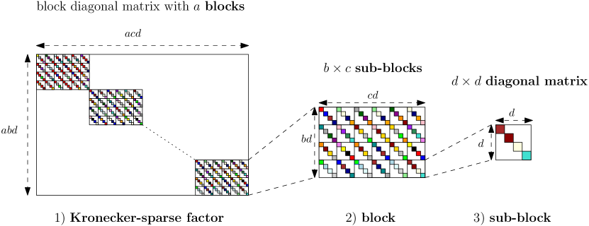
Figure 1: Illustration of the support of a factor with pattern ${\boldsymbol{\pi}}=(a,b,c,d)$. The colored squares indicate the indices belonging to the support. The sub-figures (1), (2), (3) illustrate respectively the concepts of factor, block and sub-block.

1.1 Problem formulation and contributions

This paper focuses on the problem of approximating a target matrix $\mathbf{A}$ by a product of structured sparse factors associated with a given architecture ${\boldsymbol{\beta}}=({\boldsymbol{\pi}}_{\ell})_{\ell=1}^{L}$:

(1) $$E^{\boldsymbol{\beta}}(\mathbf{A}):=\inf_{({\mathbf{X}}_{\ell})_{\ell=1}^{L}}\|\mathbf{A}-{\mathbf{X}}_{1}\ldots{\mathbf{X}}_{L}\|_{F}^{2}=\inf_{\mathbf{B}}\|\mathbf{A}-\mathbf{B}\|_{F}^{2},$$

where $\mathbf{B}$ is a butterfly matrix (cf. (2) below and Definition 4.5), each ${\mathbf{X}}_{\ell}$ is a factor with sparsity pattern prescribed by ${\boldsymbol{\pi}}_{\ell}$, and $\|\cdot\|_{F}$ is the Frobenius norm. We will call these factors “Kronecker-sparse factor”, due to the Kronecker-structure of their sparsity pattern. Several methods have been proposed to address this butterfly factorization problem, but we argue that they either lack guarantees of success, or only have partial guarantees. We fix this issue here by introducing a new butterfly algorithm endowed with theoretical guarantees.

Table 1: Existing architectures ${\boldsymbol{\beta}}$ in the literature. ${(\star)}$ Note that [27] did not explicitly state constraints on $(a_{\ell},b_{\ell},c_{\ell},d_{\ell})_{\ell=1}^{L}$ for deformable butterfly factorization, because they use an alternative description of the sparsity patterns of the factors. See Example 4.12 for more details.

Architectures	$L$	Size	Values of ${\boldsymbol{\beta}}=({\boldsymbol{\pi}}_{\ell})_{\ell=1}^{L}$	Chainable?
Low-rank matrix	2	$m\times n$	$(1,m,r,1)$, $(1,r,n,1)$	Yes
Monarch [4]	2	$m\times n$	$(1,p,q,m/p)$, $(q,m/p,n/q,1)$	Yes
Square dyadic butterfly [5]	any	$2^{L}\times 2^{L}$	$(2^{\ell-1},2,2,2^{L-\ell})_{\ell=1}^{L}$	Yes
($\star$) Deformable butterfly [27]	any	$m\times n$	$(a_{\ell},b_{\ell},c_{\ell},d_{\ell})_{\ell=1}^{L}$	Yes
Kaleidoscope [6]	even	$2^{L/2}\times 2^{L/2}$	${\boldsymbol{\pi}}_{\ell}=\begin{cases}(2^{\ell-1},2,2,2^{L/2-\ell})&\text{if }\ell\leq L/2\\ (2^{L-\ell},2,2,2^{\ell-L/2-1})&\text{if }\ell>L/2\\ \end{cases}$	No

More precisely, the main contributions of this paper are:

1. To introduce, via the definition of a Kronecker-sparse factor, a formal mathematical description of the “deformable butterfly factors” of [27]. While we owe [27] the original idea of extending previous butterfly factorizations, the mathematical formulation of the prescribed supports as Kronecker products is a novelty that allows a theoretical study of the corresponding butterfly factorization, as done in this paper. Moreover, our parameterization uses 4 parameters and removes the redundancy in the original 5-parameter description of deformable butterfly factors of [27]. Table 1 summarizes the main characteristics of existing butterfly architectures covered by our framework.

2. To define the chainability of an architecture ${\boldsymbol{\beta}}$ (Definition 4.11), which is basically a “stability” property that ensures that a product of Kronecker-sparse factors is still a Kronecker-sparse factor. We prove that Problem (1) admits an optimum when ${\boldsymbol{\beta}}$ is chainable (Theorem 7.11).

3. To characterize analytically the set of butterfly matrices with architecture ${\boldsymbol{\beta}}$,

   (2) $$\mathcal{B}^{{\boldsymbol{\beta}}}:=\left\{{\mathbf{X}}_{1}\ldots{\mathbf{X}}_{L}\,|\,\mathtt{supp}({\mathbf{X}}_{\ell})\subseteq\mathtt{supp}(\mathbf{S}_{{\boldsymbol{\pi}}_{\ell}})\,\ \forall\ell\in\llbracket L\rrbracket\right\},$$

   for a chainable ${\boldsymbol{\beta}}$, in terms of low-rank properties of certain submatrices of $\mathbf{A}$ (Corollary 7.9) that are equivalent to a generalization of the complementary low-rank property (Definitions F.2 and F.4).

4. To define the redundancy of a chainable architecture (Definition 4.17). Intuitively, a chainable architecture ${\boldsymbol{\beta}}$ is redundant if one can replace it with a “compressed” (non-redundant) one ${\boldsymbol{\beta}}^{\prime}$ such that $\mathcal{B}^{{\boldsymbol{\beta}}}=\mathcal{B}^{{\boldsymbol{\beta}}^{\prime}}$ (Proposition 4.24). Thus, from the perspective of accelerating linear operators, redundant architectures have no practical interest.

5. To propose a new butterfly algorithm (Algorithm 4) able to provide an approximate solution to Problem (1) for non-redundant chainable architectures. Compared to previous similar algorithms, this algorithm introduces a new orthogonalization step that is key to obtain approximation guarantees. The algorithm can be easily extended to redundant chainable architectures, with the same theoretical guarantee (see Remark 6.4).

6. To prove that, for a chainable ${\boldsymbol{\beta}}$, Algorithm 4 outputs butterfly factors $({\hat{\mathbf{X}}}_{\ell})_{\ell=1}^{L}$ such that

   (3) $$\|\mathbf{A}-{\hat{\mathbf{X}}}_{1}\ldots{\hat{\mathbf{X}}}_{L}\|_{F}\leq C_{\boldsymbol{\beta}}\cdot\inf_{{(\mathbf{X}_{\ell})_{\ell=1}^{L}}}\|\mathbf{A}-\mathbf{X}_{1}\ldots\mathbf{X}_{L}\|_{F},$$

   where $C_{\boldsymbol{\beta}}\geq 1$ depends only on ${\boldsymbol{\beta}}$ (Theorem 7.4), see Table 2 for examples. To the best of our knowledge, this is the first time such a bound is established for a butterfly approximation algorithm.

1.2 Outline

Section 2 discusses related work. Section 3 introduces some preliminaries on two-factor matrix factorization with fixed-support constraints. This is also where we setup our general notations. Section 4 formalizes the definition of deformable butterfly factorization associated with ${\boldsymbol{\beta}}$, and introduces the chainability and non-redundancy conditions for an architecture ${\boldsymbol{\beta}}$, that will be at the core of the proof of error guarantees on our proposed butterfly algorithm. Section 5 extends an existing hierarchical algorithm, currently expressed only for dyadic butterfly factorization, to any chainable ${\boldsymbol{\beta}}$. For non-redundant chainable ${\boldsymbol{\beta}}$, Section 6 introduces novel orthonormalization operations in the proposed butterfly algorithm. This allows us to establish in Section 7 our main results on the control of the approximation error and the low-rank characterization of butterfly matrices associated with chainable ${\boldsymbol{\beta}}$. Section 8 proposes some numerical experiments about the proposed butterfly algorithm. The most technical proofs are deferred to the appendices.

Table 2: The approximation ratio $C_{\boldsymbol{\beta}}$ (see Equation 3) of Algorithm 4 with a selection of chainable architectures ${\boldsymbol{\beta}}$ from Table 1.

Parameterization	Size	$L=|{\boldsymbol{\beta}}|$	$C_{\boldsymbol{\beta}}$ in (22) - Theorem 7.4	$C_{\boldsymbol{\beta}}$ in (23) - Theorem 7.4
Low rank matrix	$m\times n$	2	$1$	$1$
Monarch [4]	$m\times n$	2	$1$	$1$
Square dyadic butterfly [5]	$n\times n$	$\log n$	$\log n-1$	$\sqrt{\log n-1}$

2 Related work

Several methods have been proposed to address the butterfly factorization problem (1), but we argue that they either lack guarantees of success, or only have partial guarantees.

First-order methods. Optimization methods based on gradient descent [5] or alternating least squares [27] are not suitable for Problem (1) and lack guarantees of success, because of the non-convexity of the objective function. In fact, the problem of approximating a given matrix by the product of factors with fixed-support constraints, as it is the case for (1), is generally NP-hard and might even lead to numerical instability even for $L=2$ factors, as shown in [18]. In contrast, we show that the minimum of (1) always exists for chainable ${\boldsymbol{\beta}}$.

Hierarchical approach for butterfly factorization. For the specific choice of ${\boldsymbol{\beta}}$ corresponding to a square dyadic butterfly factorization, i.e., with the architecture ${\boldsymbol{\beta}}=(2^{\ell-1},2,2,2^{L-\ell})_{\ell=1}^{L}$, there exists an efficient hierarchical algorithm for Problem (1), endowed with exact recovery guarantees [20, 44]. The hierarchical approach performs successive two-factor matrix factorizations, until the desired number of factors $L$ is obtained. In the case of square dyadic butterfly factorization, it is shown that each two-factor matrix factorization in the hierarchical procedure can be solved optimally by computing the best rank-one approximation of some specific submatrices [18], which leads to an overall $\mathcal{O}(n^{2})$ complexity for approximating a matrix of size $n\times n$ with the hierarchical procedure. In fact, the hierarchical algorithm in [20, 44] can be seen as a variation of previous butterfly algorithms [23], with the novelty that it works for any hierarchical order under which successive two-layers matrix factorizations are performed, whereas existing butterfly algorithms [31, 33, 2] were only focusing on some specific hierarchical orders [29]. However, the question of controlling the approximation error of the algorithm was left as an open question in [44]. Moreover, it was not known in the literature if the hierarchical algorithm [44, 20] could be extended to architectures ${\boldsymbol{\beta}}$ beyond the square dyadic one. Both questions are answered positively here.

Butterfly algorithms and the complementary low-rank property. Butterfly algorithms [30, 31, 33, 2, 23, 24, 29] look for an approximation of a target matrix $\mathbf{A}$ by a sparse factorization $\hat{\mathbf{A}}={\mathbf{X}}_{1}\ldots{\mathbf{X}}_{L}$, assuming that $\mathbf{A}$ satisfies the so-called complementary low-rank property, formally introduced in [23]. This low-rank property assumes that the rank of certain submatrices of $\mathbf{A}$ restricted to some specific blocks is numerically low and that these blocks satisfy some conditions described by a hierarchical partitioning of the row and column indices, using the notion of cluster tree [15]. Then, the butterfly algorithm leverages this low-rank property to approximate the target matrix by a data-sparse representation, by performing successive low-rank approximation of specific submatrices. The literature in numerical analysis describes many linear operators associated with matrices satisfying the complementary low-rank property, such as kernel matrices encountered in electromagnetic or acoustic scattering problems [30, 31, 14], special function transforms [34], spherical harmonic transforms [40] or Fourier integral operators [2, 42, 24, 22, 25].

The formal definition of the complementary low-rank property currently given in the literature only considers cluster trees that are dyadic [23] or quadtrees [25]. In this work, we give a more general definition of the complementary low-rank property that considers arbitrary cluster trees. To the best of our knowledge, this allows us to give the first formal characterization of the set of matrices admitting a (deformable) butterfly factorization associated with an architecture ${\boldsymbol{\beta}}$, as defined in (2), using this extended definition of the complementary low-rank property. In particular, this shows that the definition in (2) is more general than the previous definitions of the complementary low-rank property that were restricted to dyadic trees or quadtrees [23, 25].

Existing error bounds for butterfly algorithms. Several existing butterfly algorithms [33, 2, 23, 24] are guaranteed to provide an approximation error $\|\mathbf{A}-\hat{\mathbf{A}}\|_{F}$ equal to zero, when $\mathbf{A}$ satisfies exactly the complementary low-rank property, i.e., the best low-rank approximation errors of the submatrices described by the property are exactly zero [33, 23]. However, when these submatrices are only approximately low-rank (with a positive best low-rank approximation error), existing butterfly factorization algorithms are not guaranteed to provide an approximation $\hat{\mathbf{A}}$ with the best approximation error. To the best of our knowledge, the only existing error bound in the literature is based on a butterfly algorithm that performs successive low-rank approximation of blocks $\mathbf{M}$ [29]. However, this bound does not compare the approximation error $\|\mathbf{A}-\hat{\mathbf{A}}\|_{F}$ to the best approximation error, that is, the minimal error $\|\mathbf{A}-\mathbf{A}^{*}\|_{F}$ with $\mathbf{A}^{*}$ satisfying exactly the complementary low-rank property. Moreover, in contrast to our algorithm, the algorithm proposed in [29] is not designed for butterfly factorization problems with a fixed architecture. In [29] the architecture is the result of the stopping criterion that imposes a given accuracy on the low-rank approximations of the blocks. We discuss this further in Section 7.6. In this paper, we thus propose the first error bound for butterfly factorization that compares the approximation error to the minimal approximation error, cf. (3).

3 Preliminaries

Following the hierarchical approach [21, 20, 43], our analysis of the butterfly factorization problem (1) with multiple factors in general ($L\geq 2$) relies on the analysis of the simplest setting with only $L=2$ factors. This setting is studied in [18] and after setting up our general notations we recall some important results that will be used in the rest of the paper.

3.1 Notations

The set $\llbracket a,b\rrbracket$ is the set of integers $\{a,a+1,\ldots,b\}$ for $a\leq b$, and $\llbracket a\rrbracket:=\llbracket 1,a\rrbracket$. The notation $a\mid b$ means that $a$ divides $b$. $A\times B$ is the Cartesian product of two sets $A$ and $B$. $|A|$ is the cardinal of a set $A$. By abuse of notation, for any matrix $\mathbf{X}$ and any binary matrix $\mathbf{S}$, the support constraint $\mathtt{supp}(\mathbf{X})\subseteq\mathtt{supp}(\mathbf{S})$ is simply written as $\mathtt{supp}(\mathbf{X})\subseteq\mathbf{S}$. $\mathbf{X}[i,:]$ and $\mathbf{X}[:,j]$ are the $i$-th row and the $j$-th column of $\mathbf{X}$, respectively. $\mathbf{X}[i,j]$ is the entry of $\mathbf{X}$ at the $i$-th row and $j$-th column. $\mathbf{X}[I,:]$ and $\mathbf{X}[:,J]$ are the submatrices of $\mathbf{X}$ restricted to a subset of row indices $I$ and a subset of column indices $J$, respectively. $\mathbf{X}[I,J]$ is the submatrix of $\mathbf{X}$ restricted to both $I$ and $J$. ${\mathbf{X}}^{\top}$ is the transposed matrix of $\mathbf{X}$. $\mathbf{0}_{m\times n}$ (resp. $\mathbf{1}_{m\times n}$) is the $m\times n$ matrix full of zeros (resp. of ones). The indicator (column) vector of a subset $R\subseteq\llbracket m\rrbracket$ is denoted $\mathbf{1}_{R}$. The rank of a matrix $\mathbf{M}$ is denoted $\mathtt{rank}(\mathbf{M})$. Finally, for any matrix $\mathbf{X}$, we denote $\varepsilon_{r}^{2}(\mathbf{X}):=\min_{\mathbf{Y}:\ \mathtt{rank}(\mathbf{Y})\leq r}\|\mathbf{X}-\mathbf{Y}\|_{F}^{2}$, and $\mathtt{rankproj}_{r}(\mathbf{X})$ is defined as the collection of all $\mathbf{Y}$ of rank at most $r$ achieving the minimum. All these matrices have the same Frobenius norm, denoted by $\|\mathtt{rankproj}_{r}(\mathbf{X})\|_{F}$.

3.2 Two-factor, fixed-support matrix factorization

Given two binary matrices $\mathbf{L},\mathbf{R}$, the problem of fixed-support matrix factorization (FSMF) with two factors is formulated as:

(4) $$\underset{(\mathbf{X},\mathbf{Y})}{\inf}\quad\|{\mathbf{A}}-\mathbf{X}\mathbf{Y}\|_{F}^{2},\;\text{with }\mathtt{supp}(\mathbf{X})\subseteq\mathbf{L},\mathtt{supp}(\mathbf{Y})\subseteq\mathbf{R}.$$

While Problem (4) is NP-hard in general [18, Theorem 2.4], it becomes tractable under certain conditions on $(\mathbf{L},\mathbf{R})$. To describe one of these conditions, we recall the following definitions.

Definition 3.1 (Rank-one contribution supports [18, 44]).

The rank-one contribution supports of two binary matrices $\mathbf{L}\in\{0,1\}^{m\times r},\mathbf{R}\in\{0,1\}^{r\times n}$ is the tuple $\varphi(\mathbf{L},\mathbf{R})$ of $r$ binary matrices defined by:

$$\varphi(\mathbf{L},\mathbf{R}):=(\mathbf{U}_{i})_{i=1}^{r},\quad\text{ where }\quad\mathbf{U}_{i}:=\mathbf{L}[{:,{i}}]\mathbf{R}[{{i},:}]\in\{0,1\}^{m\times n}.$$

Figure 2 illustrates the notion of rank-one contribution supports in Definition 3.1.

Remark 3.2.

The binary matrix $\mathbf{L}[{:,{i}}]\mathbf{R}[{{i},:}]$ for $i\in\llbracket r\rrbracket$ encodes the support constraint of $\mathbf{X}[{:,{i}}]\mathbf{Y}[{{i},:}]$ for each $(\mathbf{X},\mathbf{Y})$ such that $\mathtt{supp}(\mathbf{X})\subseteq\mathbf{L}$, $\mathtt{supp}(\mathbf{Y})\subseteq\mathbf{R}$.

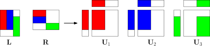
Figure 2: An example of support constraints $(\mathbf{L},\mathbf{R})$ and the supports of the corresponding rank-one contributions. Colored parts indicate indices inside the support constraints $\mathbf{L},\mathbf{R}$ and $\mathbf{U}_{i}$ for $i\in\llbracket 3\rrbracket$. $\{1,2\}$ and $\{3\}$ are the two equivalence classes (Definition 3.3).

The rank-one supports $(\mathbf{U}_{i})_{i=1}^{r}$ defines an equivalence relation and its induced equivalence classes on the set of indices $\llbracket r\rrbracket$, as illustrated in Figure 2.

Definition 3.3 (Equivalence classes of rank-one supports, representative rank-one supports [18]).

Given $\mathbf{L}\in\{0,1\}^{m\times r},\mathbf{R}\in\{0,1\}^{r\times n}$, denoting $(\mathbf{U}_{i})_{i=1}^{r}{=}\varphi(\mathbf{L},\mathbf{R})$, define an equivalence relation on the index set $\llbracket r\rrbracket$ of the rows of $\mathbf{L}$ / columns of $\mathbf{R}$ as:

$$i\sim j\iff\mathbf{U}_{i}=\mathbf{U}_{j}.$$

This yields a partition of the index set $\llbracket r\rrbracket$ into equivalence classes, denoted $\mathcal{P}(\mathbf{L},\mathbf{R})$. For each $P\in\mathcal{P}(\mathbf{L},\mathbf{R})$, denote $\mathbf{U}_{P}$ a representative rank-one support, $R_{P}\subseteq\llbracket m\rrbracket$ and $C_{P}\subseteq\llbracket n\rrbracket$ the supports of rows and columns in $\mathbf{U}_{P}$, respectively, i.e., $\mathtt{supp}(\mathbf{U}_{P})=R_{P}\times C_{P}$, and denote $|P|$ the cardinal of the equivalence class $P$.

We now recall a sufficient condition on the binary support matrices $(\mathbf{L},\mathbf{R})$ for which corresponding instances of Problem (4) can be solved in polynomial time via Algorithm 1.

Theorem 3.4 (Tractable support constraints of Problem (4) [18, Theorem 3.3]).

If all components $\mathbf{U}_{i}$ of $\varphi(\mathbf{L},\mathbf{R})$ are pairwise disjoint or identical, then Algorithm 1 yields an optimal solution of Problem (4), and the infimum of Problem (4) is :

(5) $$\inf_{\mathtt{supp}(\mathbf{X})\subseteq\mathbf{L},\mathtt{supp}(\mathbf{Y})\subseteq\mathbf{R}}\|\mathbf{A}-\mathbf{X}\mathbf{Y}\|_{F}^{2}=\sum_{P\in\mathcal{P}(\mathbf{L},\mathbf{R})}\min_{\mathbf{B},\mathtt{rank}(\mathbf{B})\leq|P|}\|\mathbf{A}[R_{P},C_{P}]-\mathbf{B}\|_{F}^{2}+c,$$

where $c:=\displaystyle\sum_{(i,j)\notin\mathtt{supp}(\mathbf{L}\mathbf{R})}\mathbf{A}[i,j]^{2}$ is a constant depending only on $(\mathbf{A},\mathbf{L},\mathbf{R})$.

Equation (5) was not proved in [18], so we provide a complete proof of Theorem 3.4 in Appendix A. The main idea is the following.

Proof 3.5 (Sketch of proof).

For $(\mathbf{X},\mathbf{Y})$ such that $\mathtt{supp}(\mathbf{X})\subseteq\mathbf{L}$ and $\mathtt{supp}(\mathbf{Y})\subseteq\mathbf{R}$:

(6) $$\|\mathbf{A}-\mathbf{X}\mathbf{Y}\|_{F}^{2}=\sum_{P\in\mathcal{P}(\mathbf{L},\mathbf{R})}\|\mathbf{A}[R_{P},C_{P}]-\mathbf{X}[R_{P},P]\mathbf{Y}[P,C_{P}]\|_{F}^{2}+c,$$

because the fact that the components $\mathbf{U}_{i}$ of $\varphi(\mathbf{L},\mathbf{R})$ are pairwise disjoint or identical implies that the blocks of indices $R_{P}\times C_{P}$ are pairwise disjoint. Thus, minimizing the left-hand-side is equivalent to minimizing each summand in the right-hand side, which is equivalent to finding the best rank-$|P|$ approximation of the matrix $\mathbf{A}[R_{P},C_{P}]$ for each $P\in\mathcal{P}(\mathbf{L},\mathbf{R})$.

Remark 3.6.

Best low-rank approximation in line 3 of Algorithm 1 can be computed via truncated singular value decomposition (SVD). Note that the definition of $\hat{\mathbf{H}},\hat{\mathbf{K}}$ in this line is not unique, because, for instance, the product $\hat{\mathbf{H}}\hat{\mathbf{K}}$ is invariant to some rescaling of columns and rows.

Algorithm 1 Two-factor fixed-support matrix factorization

0:  $\mathbf{A}\in\mathbb{C}^{m\times n}$, $\mathbf{L}\in\{0,1\}^{m\times r}$, $\mathbf{R}\in\{0,1\}^{r\times n}$

0:  $(\mathbf{X},\mathbf{Y})$ such that $\mathtt{supp}(\mathbf{X})\subseteq\mathbf{L}$, $\mathtt{supp}(\mathbf{Y})\subseteq\mathbf{R}$

1:  $(\mathbf{X},\mathbf{Y})\leftarrow(\mathbf{0}_{m\times r},\mathbf{0}_{r\times n})$

2:  for $P\in\mathcal{P}(\mathbf{L},\mathbf{R})$ (cf. Definition 3.3) do

3:     $(\mathbf{X}[R_{P},P],\mathbf{Y}[P,C_{P}])\leftarrow$ $(\hat{\mathbf{H}},\hat{\mathbf{K}})\in\underset{\begin{subarray}{c}\mathbf{H}\in\mathbb{C}^{|R_{P}|\times|P|}\\ \mathbf{K}\in\mathbb{C}^{|P|\times|C_{P}|}\end{subarray}}{\arg\min}\|\mathbf{A}[R_{P},C_{P}]-\mathbf{H}\mathbf{K}\|_{F}$

4:  end for

5:  return  $(\mathbf{X},\mathbf{Y})$

4 Deformable butterfly factorization

This section presents a mathematical formulation of the deformable butterfly factorization [27] associated with a sequence of patterns ${\boldsymbol{\beta}}:=({\boldsymbol{\pi}}_{\ell})_{\ell=1}^{L}$ called an architecture. We then introduce the notions of chainability and non-redundancy of an architecture, that are crucial conditions for constructing a butterfly algorithm for Problem (1) with error guarantees.

4.1 A mathematical formulation for Kronecker-sparse factors

Many butterfly factorizations [5, 6, 20, 44, 4, 27] take the form $\mathbf{A}={\mathbf{X}}_{1}\ldots{\mathbf{X}}_{L}$ with $\mathtt{supp}({\mathbf{X}}_{\ell})\subseteq\mathbf{I}_{a_{\ell}}\otimes\mathbf{1}_{b_{\ell}\times c_{\ell}}\otimes\mathbf{I}_{d_{\ell}}$ for $\ell\in\llbracket L\rrbracket$, for some parameters $(a_{\ell},b_{\ell},c_{\ell},d_{\ell})_{\ell=1}^{L}$, cf. Section 1. We therefore introduce the following definition.

Definition 4.1 (Kronecker-sparse factors and their sparsity patterns).

For $a,b,c,d\in\mathbb{N}$, a Kronecker-sparse factor of pattern $\boldsymbol{\pi}:={(a,b,c,d)}$ (or $\boldsymbol{\pi}$-factor) is a matrix in $\mathbb{R}^{m\times n}$ or $\mathbb{C}^{m\times n}$, where $m:=abd$, $n:=acd$, such that its support is included in $\mathbf{S}_{{\boldsymbol{\pi}}}:=\mathbf{I}_{a}\otimes\mathbf{1}_{b\times c}\otimes\mathbf{I}_{d}\in\{0,1\}^{m\times n}$. The tuple $\boldsymbol{\pi}$ will be called an elementary Kronecker-sparse pattern, or simply a pattern. The set of all $\boldsymbol{\pi}$-factors is denoted by $\Sigma^{{\boldsymbol{\pi}}}$.

Figure 1 illustrates the support of a ${\boldsymbol{\pi}}$-factor, for a given pattern ${\boldsymbol{\pi}}=(a,b,c,d)$. A ${\boldsymbol{\pi}}$-factor matrix is block diagonal with $a$ blocks in total. By definition, each block in the diagonal has support included in $\mathbf{1}_{b\times c}\otimes\mathbf{I}_{d}$. Thus, each block is a block matrix of size $b\times c$, where each sub-block is a diagonal matrix of size $d\times d$.

Example 4.2.

The following matrices are ${\boldsymbol{\pi}}$-factors for certain choices of ${\boldsymbol{\pi}}$.

1. Dense matrix: Any matrix of size $m\times n$ is a $(1,m,n,1)$-factor.

2. Diagonal matrix: Any diagonal matrix of size $m\times m$ is either a $(m,1,1,1)$-factor or $(1,1,1,m)$-factor.

1. Factors in a square dyadic butterfly factorization [5, 6, 20, 44]: the pattern of the $\ell$-th factor is ${\boldsymbol{\pi}}_{\ell}=(2^{\ell-1},2,2,2^{L-\ell})$ for $\ell\in\llbracket L\rrbracket$.

2. Factors in a Monarch factorization [4]: the patterns of the two factors are ${\boldsymbol{\pi}}_{1}=(1,p,q,m/p)$, ${\boldsymbol{\pi}}_{2}=(q,m/p,n/q,1)$ for $p,q$ such that $p\mid m$ and $r\mid n$.

Lemma 4.3 (Sparsity level of a $\boldsymbol{\pi}$-factor).

For ${\boldsymbol{\pi}}=(a,b,c,d)$, the number of nonzero entries of a $\boldsymbol{\pi}$-factor of size $m\times n$ is at most $\|{\boldsymbol{\pi}}\|_{0}:=abcd=mc=nb$.

Proof 4.4.

The cardinal of $\mathtt{supp}(\mathbf{I}_{a}\otimes\mathbf{1}_{b\times c}\otimes\mathbf{I}_{d})$ is $abcd=mc=nb=\frac{mn}{ad}$.

A ${\boldsymbol{\pi}}$-factor is sparse if it has few nonzero entries compared to its size, i.e., if $\|\boldsymbol{\pi}\|_{0}\ll mn$, or equivalently if $ad\gg\mathcal{O}(1)$. Given a number of factors $L\geq 1$, a sequence of patterns ${\boldsymbol{\beta}}:=({\boldsymbol{\pi}}_{\ell})_{\ell=1}^{L}$ parameterizes the set

(7) $$\Sigma^{{\boldsymbol{\beta}}}:=\Sigma^{{\boldsymbol{\pi}}_{1}}\times\ldots\times\Sigma^{{\boldsymbol{\pi}}_{L}}$$

of $L$-tuples of ${\boldsymbol{\pi}}_{\ell}$-factors, $\ell=1,\ldots,L$. Since we are interested in matrix products ${\mathbf{X}}_{1}\ldots{\mathbf{X}}_{L}$ for $({\mathbf{X}}_{\ell})_{\ell=1}^{L}\in\Sigma^{{\boldsymbol{\beta}}}$, we will only consider sequences of patterns ${\boldsymbol{\beta}}$ such that the size of ${\mathbf{X}}_{\ell}\in\Sigma^{{\boldsymbol{\pi}}_{\ell}}$ and ${\mathbf{X}}_{\ell+1}\in\Sigma^{{\boldsymbol{\pi}}_{\ell+1}}$ are compatible for computing the matrix product ${\mathbf{X}}_{\ell}{\mathbf{X}}_{\ell+1}$, for each $\ell\in\llbracket L-1\rrbracket$. In other words, we require that the sequence of patterns ${\boldsymbol{\beta}}$ satisfies:

(8) $$\forall\ell\in\llbracket L-1\rrbracket,\quad\underbrace{a_{\ell}c_{\ell}d_{\ell}}_{n_{\ell}}=\underbrace{a_{\ell+1}b_{\ell+1}d_{\ell+1}}_{m_{\ell+1}}.$$

Therefore, under assumption (8), a sequence ${\boldsymbol{\beta}}$ can describe a factorization of the type $\mathbf{A}={\mathbf{X}}_{1}\ldots{\mathbf{X}}_{L}$ such that $({\mathbf{X}}_{\ell})_{\ell=1}^{L}\in\Sigma^{{\boldsymbol{\beta}}}$. We introduce the following terminology for such a sequence.

Definition 4.5 (Butterfly architecture and butterfly matrices).

A sequence of patterns ${\boldsymbol{\beta}}:=(\boldsymbol{\pi}_{\ell})_{\ell=1}^{L}$ is called a (deformable) butterfly architecture, or simply an architecture, when it satisfies (8). By analogy with deep networks, the number of factors is called the depth of the chain and denoted by $|{\boldsymbol{\beta}}|:=L$ and, using the notation $\|{\boldsymbol{\pi}}\|_{0}$ from Lemma 4.3, the number of parameters is denoted by

$$\|{\boldsymbol{\beta}}\|_{0}:=\sum_{\ell=1}^{L}\|{\boldsymbol{\pi}}_{\ell}\|_{0}.$$

For any architecture ${\boldsymbol{\beta}}$, $\mathcal{B}^{{\boldsymbol{\beta}}}$ is the set of (deformable) butterfly matrices associated with ${\boldsymbol{\beta}}$, as defined in (2). We also say that any $\mathbf{A}\in\mathcal{B}^{{\boldsymbol{\beta}}}$ admits an exact (deformable) butterfly factorization associated with the architecture ${\boldsymbol{\beta}}$. Table 1 describes existing architectures fitting our framework.

The rest of this section introduces two important properties of an architecture ${\boldsymbol{\beta}}$:

• Chainability will be shown (Theorem 7.11) to ensure the existence of an optimum in (1), so that we can replace “$\inf$” by “$\min$” in (1). We also show that, for any chainable architecture, one can exploit a hierarchical algorithm (Algorithm 3) that extends an algorithm from [20, 43] to compute an approximate solution to Problem (1).

• Non-redundancy is an additional property satisfied by some chainable architectures ${\boldsymbol{\beta}}$, that allows us to insert orthonormalization steps in the hierarchical algorithm, in order to control the approximation error for Problem (1) in the sense of (3). Non-redundancy plays the role of an intermediate tool to design and analyze our algorithms. However, it should not be treated as an additional hypothesis, because we do propose a factorization method (cf. Remark 6.4), endowed with error guarantees, for any chainable architecture, whether redundant or not.

Both conditions are first defined for the most basic architectures ${\boldsymbol{\beta}}$ of depth $|{\boldsymbol{\beta}}|=2$, before being generalized to architectures ${\boldsymbol{\beta}}$ of arbitrary depth $L\geq 2$.

4.2 Chainability

We start by defining this condition in the case of architectures of depth $L=2$. This definition is primarily introduced to ensure a key “stability” property given next in Proposition 4.8, which will have many nice consequences.

Definition 4.6 (Chainable pair of patterns, operator $*$ on patterns).

Two patterns ${\boldsymbol{\pi}}_{1}:=(a_{1},b_{1},c_{1},d_{1})$ and ${\boldsymbol{\pi}}_{2}:=(a_{2},b_{2},c_{2},d_{2})$ are chainable if:

1. $\frac{a_{1}c_{1}}{a_{2}}=\frac{b_{2}d_{2}}{d_{1}}$ and this quantity, denoted $r({\boldsymbol{\pi}}_{1},{\boldsymbol{\pi}}_{2})$, is an integer;

2. $a_{1}\mid a_{2}$ and $d_{2}\mid d_{1}$.

We also say that the pair $({\boldsymbol{\pi}}_{1},{\boldsymbol{\pi}}_{2})$ is chainable. Observe that we always have $r({\boldsymbol{\pi}}_{1},{\boldsymbol{\pi}}_{2})=c_{1}(a_{1}/a_{2})=b_{2}(d_{2}/d_{1})\leq\min(b_{2},c_{1})$, and $a_{1}c_{1}d_{1}=a_{2}b_{2}d_{2}$. We define the operator $*$ on the set of chainable pairs of patterns as follows: if $({\boldsymbol{\pi}}_{1},{\boldsymbol{\pi}}_{2})$ is chainable, then

(9) $${\boldsymbol{\pi}}_{1}*{\boldsymbol{\pi}}_{2}:=\left(a_{1},\frac{b_{1}d_{1}}{d_{2}},\frac{a_{2}c_{2}}{a_{1}},d_{2}\right)\in\mathbb{N}^{4}.$$

Note that even though the definition of $r({\boldsymbol{\pi}}_{1},{\boldsymbol{\pi}}_{2})$ involves the quotient $a_{1}/a_{2}$ (and $d_{2}/d_{1}$), assumption 2 in Definition 4.6 is indeed that $a_{1}$ divides $a_{2}$ (and $d_{2}$ divides $d_{1}$).

Remark 4.7.

The order $({\boldsymbol{\pi}}_{1},{\boldsymbol{\pi}}_{2})$ in the definition matters, i.e., this property is not symmetric: the chainability of $({\boldsymbol{\pi}}_{1},{\boldsymbol{\pi}}_{2})$ does not imply that of $({\boldsymbol{\pi}}_{2},{\boldsymbol{\pi}}_{1})$. Moreover, by the first condition of Definition 4.6, a chainable pair is indeed an architecture in the sense of Definition 4.5.

Definition 4.6 comes with the following two key results.

Proposition 4.8.

If $({\boldsymbol{\pi}}_{1},{\boldsymbol{\pi}}_{2})$ is chainable, then:

(10) $$\mathbf{S}_{{\boldsymbol{\pi}}_{1}}\mathbf{S}_{{\boldsymbol{\pi}}_{2}}=r({\boldsymbol{\pi}}_{1},{\boldsymbol{\pi}}_{2})\mathbf{S}_{{\boldsymbol{\pi}}_{1}*{\boldsymbol{\pi}}_{2}}.$$

The proof is deferred to Section B.1. The equality (10) was proved in [44, Lemma 3.4] for the choice ${\boldsymbol{\pi}}_{1}=(2^{\ell-1},2,2,2^{L-\ell})$ and ${\boldsymbol{\pi}}_{2}=(2^{\ell},2,2,2^{L-\ell-1})$, for any integer $L\geq 2$ and $\ell\in\llbracket L-1\rrbracket$. Proposition 4.8 extends (10) to all chainable pairs $({\boldsymbol{\pi}}_{1},{\boldsymbol{\pi}}_{2})$.

Chainability and Definition 4.1 imply that $\forall({\mathbf{X}}_{1},{\mathbf{X}}_{2})\in\Sigma^{{\boldsymbol{\pi}}_{1}}\times\Sigma^{{\boldsymbol{\pi}}_{2}},\,{\mathbf{X}}_{1}{\mathbf{X}}_{2}\in\Sigma^{({\boldsymbol{\pi}}_{1}*{\boldsymbol{\pi}}_{2})}$, i.e., a product of Kronecker-sparse factors with chainable patterns $({\boldsymbol{\pi}}_{1},{\boldsymbol{\pi}}_{2})$ is still a Kronecker-sparse factor, with pattern ${\boldsymbol{\pi}}_{1}*{\boldsymbol{\pi}}_{2}$. Moreover, the matrix supports corresponding to a pair of chainable patterns also satisfy useful many interesting properties related to Definition 3.3 and Theorem 3.4, as shown in the following result proved in Section B.2:

Lemma 4.9.

If ${\boldsymbol{\beta}}:=({\boldsymbol{\pi}}_{1},{\boldsymbol{\pi}}_{2})$ is chainable then (with the notations of Definition 3.3) for each $P\in\mathcal{P}(\mathbf{S}_{{\boldsymbol{\pi}}_{1}},\mathbf{S}_{{\boldsymbol{\pi}}_{2}})$ we have

1. $R_{P}=\mathtt{supp}(\mathbf{S}_{{\boldsymbol{\pi}}_{1}}[{:,{i}}])$ and $C_{P}=\mathtt{supp}(\mathbf{S}_{{\boldsymbol{\pi}}_{2}}[{{i},:}])$ for every $i\in P$.

2. The sets $R_{P}\times C_{P}$, $P\in\mathcal{P}(\mathbf{S}_{{\boldsymbol{\pi}}_{1}},\mathbf{S}_{{\boldsymbol{\pi}}_{2}})$ are pairwise disjoint.

3. $|P|=r({\boldsymbol{\pi}}_{1},{\boldsymbol{\pi}}_{2})$, $|R_{P}|=b_{1}$ and $|C_{P}|=c_{2}$ (with ${\boldsymbol{\pi}}_{i}=(a_{i},b_{i},c_{i},d_{i})$).

4. $\mathtt{supp}(\mathbf{S}_{{\boldsymbol{\pi}}_{1}*{\boldsymbol{\pi}}_{2}})=\mathtt{supp}(\mathbf{S}_{{\boldsymbol{\pi}}_{1}}\mathbf{S}_{{\boldsymbol{\pi}}_{2}})=\cup_{P\in\mathcal{P}}R_{P}\times C_{P}$.

Lemma 4.10 (Associativity of $*$).

If $({\boldsymbol{\pi}}_{1},{\boldsymbol{\pi}}_{2})$ and $({\boldsymbol{\pi}}_{2},{\boldsymbol{\pi}}_{3})$ are chainable, then

1. $({\boldsymbol{\pi}}_{1},{\boldsymbol{\pi}}_{2}*{\boldsymbol{\pi}}_{3})$ and $({\boldsymbol{\pi}}_{1}*{\boldsymbol{\pi}}_{2},{\boldsymbol{\pi}}_{3})$ are chainable;

2. $r({\boldsymbol{\pi}}_{1},{\boldsymbol{\pi}}_{2}*{\boldsymbol{\pi}}_{3})=r({\boldsymbol{\pi}}_{1},{\boldsymbol{\pi}}_{2})$ and $r({\boldsymbol{\pi}}_{1}*{\boldsymbol{\pi}}_{2},{\boldsymbol{\pi}}_{3})=r({\boldsymbol{\pi}}_{2},{\boldsymbol{\pi}}_{3})$;

3. ${\boldsymbol{\pi}}_{1}*({\boldsymbol{\pi}}_{2}*{\boldsymbol{\pi}}_{3})=({\boldsymbol{\pi}}_{1}*{\boldsymbol{\pi}}_{2})*{\boldsymbol{\pi}}_{3}$.

The proof of Lemma 4.10 is deferred to Section B.3. We can now extend the definition of chainability to a general architecture ${\boldsymbol{\beta}}$ of arbitrary depth $L\geq 1$.

Definition 4.11 (Chainable architecture).

An architecture ${\boldsymbol{\beta}}:=({\boldsymbol{\pi}}_{\ell})_{\ell=1}^{L}$, $L\geq 2$, is chainable if ${\boldsymbol{\pi}}_{\ell}$ and ${\boldsymbol{\pi}}_{\ell+1}$ are chainable for each $\ell\in\llbracket L-1\rrbracket$ in the sense of Definition 4.6. We then denote $\mathbf{r}({\boldsymbol{\beta}})=(r({\boldsymbol{\pi}}_{\ell},{\boldsymbol{\pi}}_{\ell+1}))_{\ell=1}^{L-1}\in\mathbb{N}^{L-1}$. By convention any architecture of depth $L=1$ is also chainable.

Example 4.12.

One can check that the square dyadic butterfly architecture (resp. the Monarch architecture), cf. Example 4.2, are chainable, with $\mathbf{r}({\boldsymbol{\beta}})=(1,\ldots,1)$ (resp. $\mathbf{r}({\boldsymbol{\beta}})=(1)$). They are particular cases of the $5$-parameter deformable butterfly architecture of [27], which is chainable with $\mathbf{r}({\boldsymbol{\beta}})=(1,\ldots,1)$. In contrast, the Kaleidoscope architecture of depth $2L$ with $L\geq 2$ of Table 1 is not chainable, because for $\ell={L+1}$ we have ${\boldsymbol{\pi}}_{\ell}={(2^{L-1},2,2,1)}$, ${\boldsymbol{\pi}}_{\ell+1}={(2^{L-2},2,2,2)}$, and this pair is not chainable since $2^{L-1}$ does not divide $2^{L-2}$.

We state in the following some useful properties of chainable architectures.

Lemma 4.13.

If ${\boldsymbol{\beta}}=({\boldsymbol{\pi}}_{\ell})_{\ell=1}^{L}$ with $L\geq 2$ is chainable then $\mathcal{B}^{{\boldsymbol{\beta}}}\subseteq\Sigma^{({\boldsymbol{\pi}}_{1}*\ldots*{\boldsymbol{\pi}}_{L})}$, with

(11) $${\boldsymbol{\pi}}_{1}*\ldots*{\boldsymbol{\pi}}_{L}=\left(a_{1},\frac{b_{1}d_{1}}{d_{L}},\frac{a_{L}c_{L}}{a_{1}},d_{L}\right).$$

Proof 4.14 (Partial proof).

Proposition 4.8 yields $\mathcal{B}^{{\boldsymbol{\beta}}}\subseteq\Sigma^{({\boldsymbol{\pi}}_{1}*\ldots*{\boldsymbol{\pi}}_{L})}$ when $L=2$. This extends to any $L\geq 2$ by an induction. We prove (11) in Section B.4.

Remark 4.15.

As a consequence of this lemma, if the first pattern ${\boldsymbol{\pi}}_{1}$ of a chainable architecture ${\boldsymbol{\beta}}$ satisfies $a_{1}>1$ then all matrices in $\mathcal{B}^{{\boldsymbol{\beta}}}$ have a support included in $\mathbf{S}_{{\boldsymbol{\pi}}_{1}*\ldots*{\boldsymbol{\pi}}_{L}}$, which has zeroes outside its main block diagonal structure (see Figure 1). A similar remark holds when $d_{L}>1$, and in both cases we conclude that $\mathcal{B}^{{\boldsymbol{\beta}}}$ does not contain any dense matrix where all entries are nonzero. In contrast, when $a_{1}=d_{L}=1$, it is known for specific architectures that some dense matrices do belong to $\mathcal{B}^{{\boldsymbol{\beta}}}$. This is notably the case when ${\boldsymbol{\beta}}$ is the square dyadic butterfly architecture or the Monarch architecture (see Example 4.2): then we have ${\boldsymbol{\pi}}_{1}*\ldots*{\boldsymbol{\pi}}_{L}=(a_{1},m,n,d_{L})=(1,m,n,1)$ for some integers $m,n$, and indeed the Hadamard (or the DFT matrix, up to bit-reversal permutation of its columns, cf. [5]) is a dense matrix belonging to $\mathcal{B}^{{\boldsymbol{\beta}}}$.

Next we state an essential property of chainable architectures. It builds on and extends Lemma 4.10, and corresponds to a form of stability under pattern multiplication that will serve as a cornerstone to support the introduction of hierarchical algorithms.

Lemma 4.16.

If ${\boldsymbol{\beta}}=({\boldsymbol{\pi}}_{\ell})_{\ell=1}^{L}$ is chainable then for each $1\leq q\leq s<t\leq L$, the patterns $({\boldsymbol{\pi}}_{q}*\ldots*{\boldsymbol{\pi}}_{s})$ and $({\boldsymbol{\pi}}_{s+1}*\ldots*{\boldsymbol{\pi}}_{t})$ are well-defined and chainable with $r({\boldsymbol{\pi}}_{q}*\ldots*{\boldsymbol{\pi}}_{s},{\boldsymbol{\pi}}_{s+1}*\ldots*{\boldsymbol{\pi}}_{t})=r({\boldsymbol{\pi}}_{s},{\boldsymbol{\pi}}_{s+1})$.

The proof is deferred to Section B.5.

4.3 Non-redundancy

A first version of our proposed hierarchical factorization algorithm (expressed recursively in Algorithm 3) will be applicable to any chainable architecture ${\boldsymbol{\beta}}$. However, establishing approximation guarantees as in Equation 3 will require a variant of this algorithm (Algorithm 4) involving certain orthonormalization steps, which are only well-defined if the architecture ${\boldsymbol{\beta}}$ satisfies an additional non-redundancy condition. Fortunately, any redundant architecture ${\boldsymbol{\beta}}$ can be transformed (Proposition 4.24) into an expressively equivalent architecture ${\boldsymbol{\beta}}^{\prime}$ (i.e., $\mathcal{B}^{{\boldsymbol{\beta}}^{\prime}}=\mathcal{B}^{{\boldsymbol{\beta}}}$) with reduced number of parameters ($\|{\boldsymbol{\beta}}^{\prime}\|_{0}\leq\|{\boldsymbol{\beta}}^{\prime}\|_{0}$) thanks to Algorithm 2 below. This will be instrumental in introducing the proving approximation guarantees of the final butterfly algorithm Algorithm 4 applicable to any (redundant or not) chainable architecture.

To define redundancy of an architecture we begin by considering elementary pairs.

Definition 4.17 (Redundant architecture).

A chainable pair of patterns ${\boldsymbol{\pi}}_{1}=(a_{1},b_{1},c_{1},d_{1})$ and ${\boldsymbol{\pi}}_{2}=(a_{2},b_{2},c_{2},d_{2})$ is redundant if $r({\boldsymbol{\pi}}_{1},{\boldsymbol{\pi}}_{2})\geq\min(b_{1},c_{2})$ (i.e., if $a_{1}c_{1}\geq a_{2}c_{2}$ or $b_{2}d_{2}\geq b_{1}d_{1}$). A chainable architecture ${\boldsymbol{\beta}}=({\boldsymbol{\pi}}_{\ell})_{\ell=1}^{L}$, $L=|{\boldsymbol{\beta}}|\geq 1$, is redundant if there exists $\ell\in\llbracket L-1\rrbracket$ such that $({\boldsymbol{\pi}}_{\ell},{\boldsymbol{\pi}}_{\ell+1})$ is redundant. Observe that by definition, any chainable architecture with $|{\boldsymbol{\beta}}|=1$ is non-redundant.

Remark 4.18.

By Definition 4.6 we always have $r({\boldsymbol{\pi}}_{1},{\boldsymbol{\pi}}_{2})\leq\min(b_{2},c_{1})$ for a chainable pair $({\boldsymbol{\pi}}_{1},{\boldsymbol{\pi}}_{2})$, hence a redundant one satisfies $\min(b_{1},c_{2})\leq r({\boldsymbol{\pi}}_{1},{\boldsymbol{\pi}}_{2})\leq\min(b_{2},c_{1})$. A non-redundant one satisfies $r({\boldsymbol{\pi}}_{1},{\boldsymbol{\pi}}_{2})\leq\min(b_{1}-1,c_{2}-1,b_{2},c_{1})$.

Lemma 4.19.

If ${\boldsymbol{\beta}}=({\boldsymbol{\pi}}_{\ell})_{\ell=1}^{L}$ is chainable and non-redundant then, for any $1\leq r\leq s<t\leq L$, the pair $({\boldsymbol{\pi}}_{q}*\ldots*{\boldsymbol{\pi}}_{s},{\boldsymbol{\pi}}_{s+1}*\ldots*{\boldsymbol{\pi}}_{t})$ is chainable and non-redundant.

The proof is deferred to Section B.6.

Example 4.20.

The architecture ${\boldsymbol{\beta}}:=({\boldsymbol{\pi}}_{1},{\boldsymbol{\pi}}_{2}):=\left((1,m,r,1),(1,r,n,1)\right)$ is chainable, with $r({\boldsymbol{\pi}}_{1},{\boldsymbol{\pi}}_{2})=r$. The set $\mathcal{B}^{{\boldsymbol{\beta}}}$ is the set of $m\times n$ matrices of rank at most $r$. $({\boldsymbol{\pi}}_{1},{\boldsymbol{\pi}}_{2})$ is redundant if $r\geq\min(m,n)$. We observe that on this example redundancy corresponds to the case where $\mathcal{B}^{{\boldsymbol{\beta}}}$ is the set of all $m\times n$ matrices.

A (chainable and) redundant architecture is as expressive as a smaller chainable architecture with less parameters. This is first proved for pairs, i.e., ${\boldsymbol{\beta}}:=({\boldsymbol{\pi}}_{1},{\boldsymbol{\pi}}_{2})$.

In order to do this we need the following result, characterizing precisely the set of matrices $\mathcal{B}^{{\boldsymbol{\beta}}}=\{\mathbf{X}_{1}\mathbf{X}_{2}\,|\,\mathbf{X}_{i}\in\Sigma^{{\boldsymbol{\pi}}_{i}},i\in\llbracket 2\rrbracket\}$ as the set of matrices having a support included in $\mathbf{S}_{{\boldsymbol{\pi}}_{1}*{\boldsymbol{\pi}}_{2}}$ and with selected low-rank blocks. It is proved in Section B.7.

Lemma 4.21.

Let ${\boldsymbol{\beta}}:=({\boldsymbol{\pi}}_{1},{\boldsymbol{\pi}}_{2})$ be chainable, and (with the notations of Definition 3.3) consider the following set of matrices of size equal to those in $\mathcal{B}^{{\boldsymbol{\beta}}}$:

(12) $$\mathcal{A}^{{\boldsymbol{\beta}}}:=\{\mathbf{A}:\mathtt{rank}\big{(}\mathbf{A}[R_{P},C_{P}]\big{)}\leq r({\boldsymbol{\pi}}_{1},{\boldsymbol{\pi}}_{2}),\ \forall P\in\mathcal{P}(\mathbf{S}_{{\boldsymbol{\pi}}_{1}},\mathbf{S}_{{\boldsymbol{\pi}}_{2}})\}.$$

We have

(13) $$\mathcal{B}^{{\boldsymbol{\beta}}}=\Sigma^{{\boldsymbol{\pi}}_{1}*{\boldsymbol{\pi}}_{2}}\cap\mathcal{A}^{{\boldsymbol{\beta}}}.$$

Lemma 4.22.

Consider a chainable pair ${\boldsymbol{\beta}}=({\boldsymbol{\pi}}_{1},{\boldsymbol{\pi}}_{2})$. If ${\boldsymbol{\beta}}$ is redundant, then the single-factor architecture ${\boldsymbol{\beta}}^{\prime}=({\boldsymbol{\pi}}_{1}*{\boldsymbol{\pi}}_{2})$ satisfies :

1. $\mathcal{B}^{{\boldsymbol{\beta}}}=\Sigma^{{\boldsymbol{\pi}}_{1}*{\boldsymbol{\pi}}_{2}}=\mathcal{B}^{{\boldsymbol{\beta}}^{\prime}}$.

2. $\|{\boldsymbol{\beta}}^{\prime}\|_{0}=\|{\boldsymbol{\pi}}_{1}*{\boldsymbol{\pi}}_{2}\|_{0}<\|{\boldsymbol{\pi}}_{1}\|_{0}+\|{\boldsymbol{\pi}}_{2}\|_{0}=\|{\boldsymbol{\beta}}\|_{0}$.

Proof 4.23.

By Lemma 4.21 we have $\mathcal{B}^{{\boldsymbol{\beta}}}=\Sigma^{{\boldsymbol{\pi}}_{1}*{\boldsymbol{\pi}}_{2}}\cap\mathcal{A}^{{\boldsymbol{\beta}}}$ and by Lemma 4.9 we have $|R_{P}|=b_{1},|C_{P}|=c_{2}$ for each $P\in\mathcal{P}(\mathbf{S}_{{\boldsymbol{\pi}}_{1}},\mathbf{S}_{{\boldsymbol{\pi}}_{2}})$. The first claim follows from the fact that $\mathcal{A}^{{\boldsymbol{\beta}}}$ is the set of all matrices of appropriate size: indeed for any such matrix $\mathbf{A}$, the block $\mathbf{A}[R_{P},C_{P}]$ is of size $b_{1}\times c_{2}$ hence its rank is at most $\min(b_{1},c_{2})$ which is smaller than or equal to $r({\boldsymbol{\pi}}_{1},{\boldsymbol{\pi}}_{2})$ since ${\boldsymbol{\beta}}$ is redundant. By definition of $\mathcal{A}^{{\boldsymbol{\beta}}}$ this shows that $\mathbf{A}\in\mathcal{A}^{{\boldsymbol{\beta}}}$. For the second claim, by Definition 4.5 of $\|{\boldsymbol{\beta}}\|_{0}$ and $\|{\boldsymbol{\beta}}^{\prime}\|_{0}$, we only need to prove the strict inequality. Since $({\boldsymbol{\pi}}_{1},{\boldsymbol{\pi}}_{2})$ is (chainable and) redundant, we have either $a_{1}c_{1}\geq a_{2}c_{2}$ or $b_{2}d_{2}\geq b_{1}d_{1}$, hence by Lemma 4.3 and Equation 9 we obtain $\|{\boldsymbol{\pi}}_{1}*{\boldsymbol{\pi}}_{2}\|_{0}=a_{2}c_{2}b_{1}d_{1}<a_{1}c_{1}b_{1}d_{1}+a_{2}c_{2}b_{2}d_{2}=\|{\boldsymbol{\pi}}_{1}\|_{0}+\|{\boldsymbol{\pi}}_{2}\|_{0}.$

Lemma 4.22 serves as a basis to define Algorithm 2, which replaces any chainable (and possibly redundant) architecture by a “smaller” non-redundant one.

Algorithm 2 Architecture redundancy removal algorithm

0:  A chainable ${\boldsymbol{\beta}}=({\boldsymbol{\pi}}_{\ell})_{\ell=1}^{L}$

0:  A chainable and non-redundant ${\boldsymbol{\beta}}^{\prime}=({\boldsymbol{\pi}}_{\ell}^{\prime})_{\ell=1}^{L^{\prime}}$ ($1\leq L^{\prime}\leq L$)

1:  ${\boldsymbol{\beta}}^{\prime}\leftarrow{\boldsymbol{\beta}}$.

2:  while  ${\boldsymbol{\beta}}^{\prime}$ is redundant (cf. Definition 4.17) do

3:     $({\boldsymbol{\pi}}_{\ell}^{\prime})_{\ell=1}^{L^{\prime}}\leftarrow{\boldsymbol{\beta}}^{\prime}$

4:     $\ell\leftarrow$ an integer $\ell$ such that $({\boldsymbol{\pi}}_{\ell}^{\prime},{\boldsymbol{\pi}}_{\ell+1}^{\prime})$ is redundant (cf. Definition 4.17)

5:     ${\boldsymbol{\beta}}^{\prime}\leftarrow({\boldsymbol{\pi}}_{1}^{\prime},\ldots,{\boldsymbol{\pi}}_{\ell-1}^{\prime},{\boldsymbol{\pi}}_{\ell}^{\prime}*{\boldsymbol{\pi}}_{\ell+1}^{\prime},{\boldsymbol{\pi}}_{\ell+2}^{\prime},\ldots,{\boldsymbol{\pi}}_{L^{\prime}}^{\prime})$

6:  end while

7:  return  ${\boldsymbol{\beta}}^{\prime}$

Proposition 4.24.

For any chainable architecture ${\boldsymbol{\beta}}=({\boldsymbol{\pi}}_{\ell})_{\ell=1}^{L}$, Algorithm 2 stops in finitely many iterations and returns an architecture ${\boldsymbol{\beta}}^{\prime}$ such that:

1. ${\boldsymbol{\beta}}^{\prime}$ is chainable and non-redundant, and either a single factor architecture ${\boldsymbol{\beta}}^{\prime}=({\boldsymbol{\pi}}_{1}*\ldots*{\boldsymbol{\pi}}_{L})$, or a multi-factor one ${\boldsymbol{\beta}}^{\prime}=({\boldsymbol{\pi}}_{1}*\ldots*{\boldsymbol{\pi}}_{\ell_{1}},{\boldsymbol{\pi}}_{\ell_{1}+1}*\ldots*{\boldsymbol{\pi}}_{\ell_{2}},\ldots,{\boldsymbol{\pi}}_{\ell_{p}+1}*\ldots*{\boldsymbol{\pi}}_{L})$ for some indices $1\leq\ell_{1}<\ldots<\ell_{p}<L$ with $p\in\llbracket 1,L-1\rrbracket$;

2. $\mathcal{B}^{{\boldsymbol{\beta}}^{\prime}}=\mathcal{B}^{{\boldsymbol{\beta}}}$;

3. $\|{\boldsymbol{\beta}}^{\prime}\|_{0}\leq\|{\boldsymbol{\beta}}\|_{0}$.

Proof 4.25.

Algorithm 2 terminates since $|{\boldsymbol{\beta}}^{\prime}|$ decreases at each iteration. At each iteration, the updated ${\boldsymbol{\beta}}^{\prime}$ is obtained by replacing a chainable redundant pair $({\boldsymbol{\pi}}_{\ell}^{\prime},{\boldsymbol{\pi}}_{\ell+1}^{\prime})$ by a single pattern $({\boldsymbol{\pi}}_{\ell}^{\prime}*{\boldsymbol{\pi}}_{\ell+1}^{\prime})$. The architecture ${\boldsymbol{\beta}}^{\prime}$ remains chainable by Lemma 4.16 and by chainability of ${\boldsymbol{\beta}}$, hence the algorithm can continue with no error. Due to the condition of the “while” loop, the returned ${\boldsymbol{\beta}}^{\prime}$ is either non-redundant with $|{\boldsymbol{\beta}}^{\prime}|>1$, or $|{\boldsymbol{\beta}}^{\prime}|=1$ in which case it is in fact also non-redundant by Definition 4.17. This yields the first condition (a formal proof of the final form of ${\boldsymbol{\beta}}^{\prime}$ can be done by an easy but tedious induction left to the reader). Moreover, a straightforward consequence of Lemma 4.22 is that the update of ${\boldsymbol{\beta}}^{\prime}$ in line 5 does not change $\mathcal{B}^{{\boldsymbol{\beta}}^{\prime}}$, and it strictly decreases $\|{\boldsymbol{\beta}}^{\prime}\|_{0}$ if the condition of the “while” loop is met at least once (otherwise the algorithm outputs ${\boldsymbol{\beta}}^{\prime}={\boldsymbol{\beta}}$). This yields the two other properties.

In particular, Algorithm 2 applied to a redundant architecture ${\boldsymbol{\beta}}$ in Example 4.20 returns ${\boldsymbol{\beta}}^{\prime}=\left((1,m,r,1)*(1,r,n,1)\right)=\left((1,m,n,1)\right)$.

4.4 Constructing a chainable architecture for a target matrix size

It is natural to wonder what (non-redundant) chainable architectures ${\boldsymbol{\beta}}=({\boldsymbol{\pi}}_{\ell})_{\ell=1}^{L}$ allow to implement dense matrices of a prescribed size. This is the object of the next lemma, which is proved in Section B.8.

Lemma 4.26.

Consider integers $m,n,L\geq 2$. If ${\boldsymbol{\beta}}=({\boldsymbol{\pi}}_{\ell})_{\ell=1}^{L}$ is a chainable architecture such that $\mathcal{B}^{{\boldsymbol{\beta}}}$ is made of $m\times n$ matrices and contains at least one dense matrix, then there exists a factorization of $m$ (resp. of $n$) into $L$ integers $q_{\ell}$ (resp. $p_{\ell}$), $1\leq\ell\leq L$, and a sequence of $L-1$ integers $r_{\ell}$, $1\leq\ell\leq L-1$ such that: with the convention $r_{0}=r_{L}=1$, for each $1\leq\ell\leq L$ we have ${\boldsymbol{\pi}}_{\ell}=(a_{\ell},b_{\ell},c_{\ell},d_{\ell})$ with

(14) $$a_{\ell} =\prod_{j=1}^{\ell-1}p_{\ell},\quad\text{and}\ d_{\ell}=\prod_{j=\ell+1}^{L}q_{\ell},$$

(15) $$b_{\ell} =q_{\ell}r_{\ell-1},\quad\text{and}\ c_{\ell}=p_{\ell}r_{\ell}.$$

Vice-versa, any architecture defined as above with integers such that $n=\prod_{\ell=1}^{L}p_{\ell}$ and $m=\prod_{\ell=1}^{L}q_{\ell}$ is chainable, and the set $\mathcal{B}^{{\boldsymbol{\beta}}}\subseteq\mathbb{R}^{m\times n}$ contains at least one dense matrix.

The architecture ${\boldsymbol{\beta}}$ is non-redundant if, and only if, $r_{1}<q_{1}$, $r_{L-1}<p_{L}$, and

(16) $$\frac{1}{p_{\ell}}<\frac{r_{\ell}}{r_{\ell-1}}<q_{\ell},\ 2\leq\ell\leq L-1.$$

The proof of the following corollary is straightforward and left to the reader.

Corollary 4.27.

Consider integers $m,n\geq 2$ and their integer factorizations into $L\geq 2$ integers $p_{\ell},q_{\ell}$ as in Lemma 4.26.

• If $p_{\ell}\geq 2$ and $q_{\ell}\geq 2$ for every $1\leq\ell\leq L$, then there exists a choice of integers $r_{\ell}$, $1\leq\ell\leq L-1$ such that the construction of Lemma 4.26 is non-redundant.

• If either $q_{1}=1$, $p_{L}=1$, or $p_{\ell}q_{\ell}=1$ for some $2\leq\ell\leq L-1$, then no choice of $r_{\ell}$ allows us to obtain a non-redundant architecture.

As a consequence, given a matrix size $m\times n$, a chainable architecture compatible with this matrix size can be built via the following steps:

1. choosing integer sequences $\boldsymbol{p}:=(p_{\ell})_{\ell=1}^{L}$, $\boldsymbol{q}:=(q_{\ell})_{\ell=1}^{L}$ that factorize $n$ and $m$ (optionally: with the condition that $p_{\ell}\geq 2$ and $q_{\ell}\geq 2$ for every $\ell$);

2. choosing an integer sequence $\boldsymbol{r}:=(r_{\ell})_{\ell=1}^{L-1}$ (optionally: with the condition that $r_{1}<q_{1}$, $r_{L-1}<p_{L}$, and (16) holds with $r_{0}=r_{L}:=1$ by convention);

3. defining of ${\boldsymbol{\pi}}_{\ell}=(a_{\ell},b_{\ell},c_{\ell},d_{\ell})$ using (14)-(15).

Instead of imposing non-redundancy constraints, it is also possible to build a possibly redundant architecture and to exploit the redundancy removal algorithm (Algorithm 2).

Remark 4.28.

Mathematically oriented readers may notice that for prime $m$ and/or $n$ there are few compatible butterfly architectures. Extending the concepts of this paper to such dimensions would allow to cover known fast transforms for prime dimensions [38]. Nevertheless, typical matrix dimensions in practical applications are composite and lead to many more choices. For instance, the dimensions of weight matrices in the vision transformer architecture [8] are commonly 768, 1024, 1280, 3072, 4096, 5120, which enable many possible choices of chainable architectures for implementing dense matrices, beyond the Monarch architecture [4] that was used specifically to accelerate such neural networks. This will be illustrated in Section 8.3.

5 Hierarchical algorithm under the chainability condition

We show how the hierarchical algorithm in [20, 44], initially introduced for specific (square dyadic) architectures, can be directly extended to the case where ${\boldsymbol{\beta}}$ is any chainable architecture. The case where $L=|{\boldsymbol{\beta}}|=1$ is trivial since Problem (1) is then simply solved by setting $\mathbf{X}_{1}$ to be a copy of $\mathbf{A}$ where all entries outside of the prescribed support are set to zero. We thus focus on $L\geq 2$ and start with ${\boldsymbol{\beta}}$ of depth $L=2$ before considering arbitrary $L\geq 2$.

5.1 Case with $L=2$ factors

Problem (1) with an architecture ${\boldsymbol{\beta}}=({\boldsymbol{\pi}}_{1},{\boldsymbol{\pi}}_{2})$ is simply an instance of Problem (4) with $(\mathbf{L},\mathbf{R})=(\mathbf{S}_{{\boldsymbol{\pi}}_{1}},\mathbf{S}_{{\boldsymbol{\pi}}_{2}})$.

Lemma 5.1.

Consider the pair of supports $(\mathbf{L},\mathbf{R})=(\mathbf{S}_{{\boldsymbol{\pi}}_{1}},\mathbf{S}_{{\boldsymbol{\pi}}_{2}})$ associated to any (not necessarily chainable) architecture $({\boldsymbol{\pi}}_{1},{\boldsymbol{\pi}}_{2})$. The assumptions of Theorem 3.4 hold, hence for any architecture ${\boldsymbol{\beta}}$ of depth $|{\boldsymbol{\beta}}|=2$, the two-factor fixed-support matrix factorization algorithm (Algorithm 1) returns an optimal solution to the corresponding instance of Problem (1).

Proof 5.2.

As in the proof of Lemma 4.9, the column supports $\{{\mathbf{S}_{{\boldsymbol{\pi}}_{1}}}[:,j]\}_{j}$ (resp. the row supports $\{{\mathbf{S}_{{\boldsymbol{\pi}}_{2}}}[i,:]\}_{i}$) are pairwise disjoint or identical. Hence the components $\mathbf{U}_{i}$ of $\varphi(\mathbf{S}_{{\boldsymbol{\pi}}_{1}},\mathbf{S}_{{\boldsymbol{\pi}}_{2}})$ are pairwise disjoint or identical (if their column and row supports coincide).

5.2 Case with $L\geq 2$ factors

Consider now Problem (1) associated with a chainable architecture ${\boldsymbol{\beta}}$ of depth $L\coloneqq|{\boldsymbol{\beta}}|\geq 2$, and a given target matrix $\mathbf{A}$. A first proposition of hierarchical algorithm, introduced in Algorithm 3, is a direct adaptation to our framework of previous algorithms [20, 44]. It computes an approximate solution by performing successive two-factor matrix factorization in a certain hierarchical order that is described by a so-called factor-bracketing tree [44]. Further refinements of the algorithm will later be added to obtain approximation guarantees.

Definition 5.3 (Factor-bracketing tree [44]).

A factor-bracketing tree of $\llbracket L\rrbracket$ for a given integer $L$ is a binary tree such that:

• each node is an interval $\llbracket q,t\rrbracket:=\{q,q+1,\ldots,t\}$ for $1\leq q\leq t\leq L$;

• the root is $\llbracket L\rrbracket$;

• every non-leaf node $\llbracket q,t\rrbracket$ for $q<t$ has $\llbracket q,s\rrbracket$ as its left child and $\llbracket s+1,t\rrbracket$ as its right child, for a certain $s$ such that $q\leq s<t$;

• a leaf is a singleton $\llbracket q,q\rrbracket$ for some $q\in\llbracket 1,L\rrbracket$.

Such a tree has exactly $(L-1)$ non-leaf nodes and $L$ leaves.

Before exposing the limitations of Algorithm 3 and proposing fixes, let us briefly explain how it works with a focus on its main step in line 7. Consider any factor-bracketing tree $\mathcal{T}$. Algorithm 3 computes a matrix ${\mathbf{\mathbf{X}}}_{\llbracket q,t\rrbracket}\in\Sigma^{{\boldsymbol{\pi}}_{q}*\ldots*{\boldsymbol{\pi}}_{t}}$ for each node $\llbracket q,t\rrbracket$ in a recursive manner. ${\boldsymbol{\pi}}_{q}*\ldots*{\boldsymbol{\pi}}_{t}$ is well-defined for any $1\leq q\leq t\leq L$ because ${\boldsymbol{\beta}}$ is chainable. At the root node, we set ${\mathbf{\mathbf{X}}}_{\llbracket 1,L\rrbracket}:=\mathbf{A}$. At each non-leaf node $\llbracket q,t\rrbracket$ whose matrix $\mathbf{X}_{\llbracket q,t\rrbracket}$ is already computed during the hierarchical procedure, and with children $\llbracket q,s\rrbracket$ and $\llbracket s+1,t\rrbracket$, at line 7 we compute $(\mathbf{X}_{\llbracket q,s\rrbracket},\mathbf{X}_{\llbracket s+1,t\rrbracket})\in\Sigma^{{\boldsymbol{\pi}}_{q}*\ldots*{\boldsymbol{\pi}}_{s}}\times\Sigma^{{\boldsymbol{\pi}}_{s+1}*\ldots*{\boldsymbol{\pi}}_{t}}$ that is solution to the following instance of the Fixed Support Matrix Factorization Problem (4):

(17) Minimize $$\|\mathbf{X}_{\llbracket q,t\rrbracket}-\mathbf{X}_{\llbracket q,s\rrbracket}\mathbf{X}_{\llbracket s+1,t\rrbracket}\|_{F}$$

Subject to $$\mathtt{supp}(\mathbf{X}_{\llbracket q,s\rrbracket})\subseteq\mathbf{S}_{{\boldsymbol{\pi}}_{q}*\ldots*{\boldsymbol{\pi}}_{s}},$$

$$\mathtt{supp}(\mathbf{X}_{\llbracket s+1,t\rrbracket})\subseteq\mathbf{S}_{{\boldsymbol{\pi}}_{s+1}*\ldots*{\boldsymbol{\pi}}_{t}}.$$

Indeed, by Lemma 5.1, Problem (17) is solved by the two-factor fixed support matrix factorization algorithm (Algorithm 1), which yields line 7 in Algorithm 3. After computing $(\mathbf{X}_{\llbracket q,s\rrbracket},\mathbf{X}_{\llbracket s+1,t\rrbracket})$, we repeat recursively the procedure on these two matrices independently, as per lines 8 and 9, until we obtain the butterfly factors $({\mathbf{\mathbf{X}}}_{\llbracket\ell,\ell\rrbracket})_{\ell=1}^{L}\in\Sigma^{{\boldsymbol{\beta}}}$ that yield an approximation $\hat{\mathbf{A}}:={\mathbf{\mathbf{X}}}_{\llbracket 1,1\rrbracket}\ldots{\mathbf{\mathbf{X}}}_{\llbracket L,L\rrbracket}\in\mathcal{B}^{{\boldsymbol{\beta}}}$ of $\mathbf{A}$. In conclusion, Algorithm 3 is a greedy algorithm that seeks the optimal solution at each two-factor matrix factorization problem during the hierarchical procedure.

Algorithm 3 Hierarchical factorization algorithm – recursive version

0:  $\mathbf{A}\in\mathbb{C}^{m\times n}$, chainable ${\boldsymbol{\beta}}=({\boldsymbol{\pi}}_{\ell})_{\ell=1}^{L}$, factor-bracketing tree $\mathcal{T}$

0:  $\texttt{factors}\in\Sigma^{{\boldsymbol{\beta}}}$

1:  if $L=1$ then

2:     return  $(\mathbf{A}\odot\mathbf{S}_{{\boldsymbol{\pi}}_{1}})$$\triangleright${$\odot$ is the Hadamard product.}

3:  end if

4:  $\llbracket 1,s\rrbracket,\llbracket s+1,L\rrbracket\leftarrow$ two children of the root $\llbracket 1,L\rrbracket$ of $\mathcal{T}$

5:  $(\mathcal{T}_{\mathrm{left}},\mathcal{T}_{\mathrm{right}})\leftarrow$ the corresponding left and right subtrees of $\mathcal{T}$

6:  $({\boldsymbol{\pi}}_{\mathrm{left}},{\boldsymbol{\pi}}_{\mathrm{right}})\leftarrow({\boldsymbol{\pi}}_{1}*\ldots*{\boldsymbol{\pi}}_{s},{\boldsymbol{\pi}}_{s+1}*\ldots*{\boldsymbol{\pi}}_{L})$

7:   ($\mathbf{X}_{\llbracket 1,s\rrbracket},\mathbf{X}_{\llbracket s+1,L\rrbracket})\leftarrow$ Algorithm 1$(\mathbf{A},\mathbf{S}_{{\boldsymbol{\pi}}_{\mathrm{left}}},\mathbf{S}_{{\boldsymbol{\pi}}_{\mathrm{right}}})$

8:  $\texttt{left\_factors}\leftarrow$ Algorithm 3($\mathbf{X}_{\llbracket 1,s\rrbracket},({\boldsymbol{\pi}}_{1},\ldots,{\boldsymbol{\pi}}_{s}),\mathcal{T}_{\mathrm{left}}$)

9:  $\texttt{right\_factors}\leftarrow$ Algorithm 3($\mathbf{X}_{\llbracket s+1,L\rrbracket},({\boldsymbol{\pi}}_{s+1},\ldots,{\boldsymbol{\pi}}_{L}),\mathcal{T}_{\mathrm{right}}$)

10:  $\texttt{factors}\leftarrow\texttt{left\_factors}\cup\texttt{right\_factors}$

11:  return  factors

5.3 Algorithm 3 does not satisfy the theoretical guarantee (3)

However, the control of the approximation error in the form of (3) for Algorithm 3 in its current form is impossible, as illustrated in the following example.

Example 5.4.

Consider ${\boldsymbol{\beta}}=({\boldsymbol{\pi}}_{1},{\boldsymbol{\pi}}_{2},{\boldsymbol{\pi}}_{3})=\left((2^{\ell-1},2,2,2^{3-\ell})\right)_{\ell=1}^{3}$, which is the square dyadic architecture of depth $L=3$. Define $\mathbf{A}:=(\mathbf{D}\mathbf{S}_{{\boldsymbol{\pi}}_{1}})\mathbf{S}_{{\boldsymbol{\pi}}_{2}}\mathbf{S}_{{\boldsymbol{\pi}}_{3}}$ where $\mathbf{D}$ is the diagonal matrix with diagonal entries $(0,1,1,1,0,1,1,1)$. Hence, $\mathbf{A}\in\mathcal{B}^{{\boldsymbol{\beta}}}$, meaning that any algorithm with a theoretical guarantee (3) must output butterfly factors whose product is exactly $\mathbf{A}$. However, we claim that this is not the case of Algorithm 3 with the so-called left-to-right factor-bracketing tree of $\llbracket 1,3\rrbracket$ (defined as the tree where each left child is a singleton). To see why, let us apply this algorithm to $\mathbf{A}$.

1. In the first step, the hierarchical algorithm applies the two-factor fixed support matrix factorization algorithm (Algorithm 1) with input $(\mathbf{A},\mathbf{S}_{{\boldsymbol{\pi}}_{1}},\mathbf{S}_{{\boldsymbol{\pi}}_{2}*{\boldsymbol{\pi}}_{3}})$, and returns (${\mathbf{X}}_{\llbracket 1,1\rrbracket},{\mathbf{X}}_{\llbracket 2,3\rrbracket})\in\Sigma^{{\boldsymbol{\pi}}_{1}}\times\Sigma^{{\boldsymbol{\pi}}_{2}*{\boldsymbol{\pi}}_{3}}$.

2. At the second step (which is the last one), Algorithm 1 is applied to the input $(\mathbf{X}_{\llbracket 2,3\rrbracket},\mathbf{S}_{{\boldsymbol{\pi}}_{2}},\mathbf{S}_{{\boldsymbol{\pi}}_{3}})$, and returns $({\mathbf{X}}_{\llbracket 2,2\rrbracket},{\mathbf{X}}_{\llbracket 3,3\rrbracket})\in\Sigma^{{\boldsymbol{\pi}}_{2}}\times\Sigma^{{\boldsymbol{\pi}}_{3}}$.

By construction, the first and the fifth row of $\mathbf{A}$ are null, so the first step can return many possible optimal solutions $({\mathbf{X}}_{\llbracket 1,1\rrbracket},{\mathbf{X}}_{\llbracket 2,3\rrbracket})$ for the considered instance of Problem (4), such as ${\mathbf{X}}_{\llbracket 1,1\rrbracket}:=\mathbf{D}\mathbf{S}_{{\boldsymbol{\pi}}_{1}}$ and

$${\mathbf{X}}_{\llbracket 2,3\rrbracket}=\begin{pmatrix}\mathbf{B}&\mathbf{0}_{4\times 4}\\ \mathbf{0}_{4\times 4}&\mathbf{B}\end{pmatrix}\quad\text{with}\quad\mathbf{B}=\begin{pmatrix}\alpha&\beta&\gamma&\delta\\ 1&1&1&1\\ 1&1&1&1\\ 1&1&1&1\\ \end{pmatrix},$$

where the scalars $\alpha,\beta,\gamma,\delta$ can be arbitrary. Then, with the choice $(\alpha,\beta,\gamma,\delta)=(1,-1,1,-1)$, one can check that the second step of the procedure will always output ${\mathbf{X}}_{\llbracket 2,2\rrbracket}$ and ${\mathbf{X}}_{\llbracket 3,3\rrbracket}$ such that ${\mathbf{X}}_{\llbracket 2,2\rrbracket}{\mathbf{X}}_{\llbracket 3,3\rrbracket}\neq{\mathbf{X}}_{\llbracket 2,3\rrbracket}$ and ${\mathbf{X}}_{\llbracket 1,1\rrbracket}{\mathbf{X}}_{\llbracket 2,2\rrbracket}{\mathbf{X}}_{\llbracket 3,3\rrbracket}\neq\mathbf{A}$. In conclusion, this example shows that the output of Algorithm 3 cannot satisfy the theoretical guarantee (3).

The inability to establish an error bound as in (3) for Algorithm 3 is due to the ambiguity for the choice of optimal factors $({\mathbf{X}}_{\llbracket 1,s\rrbracket},{\mathbf{X}}_{\llbracket s+1,L\rrbracket})$ returned by the two-factor fixed support matrix factorization algorithm called at line 7 in Algorithm 3, cf. Remark 3.6. At each iteration, there are multiple optimal pairs of factors, and the choice at line 7 impacts subsequent factorizations in the recursive procedure. To guarantee an error bound of the type (3), Section 6 proposes a revision of Algorithm 3, where, among all the possible choices, the modified algorithm selects specific input matrices at lines 8 and 9.

6 Butterfly algorithm with error guarantees

We now propose a modification of the hierarchical algorithm (Algorithm 3) using orthonormalization operations that are novel in the context of butterfly factorization. It is based on an unrolled version of Algorithm 3 and will be endowed with error guarantees stated and proved in the next section.

6.1 Butterfly algorithm with orthonormalization

The factor-bracketing tree $\mathcal{T}$ in Algorithm 3 describes in which order the successive $L-1$ two-factor matrix factorization steps are performed, where $L:=|{\boldsymbol{\beta}}|$. An equivalent way to describe this hierarchical order is to store a permutation $\sigma:=(\sigma_{\ell})_{\ell=1}^{L-1}$ of $\llbracket L-1\rrbracket$, by saving each splitting index $s\in\llbracket L-1\rrbracket$ that corresponds to the maximum integer in the left child $\llbracket q,s\rrbracket$ of each non-leaf node $\llbracket q,t\rrbracket$ of $\mathcal{T}$ (cf. Definition 5.3). We can then propose a non-recursive version of Algorithm 3, described in Algorithm 4, where for any non-empty integer interval we use the shorthand

(18) $${\boldsymbol{\pi}}_{\llbracket p,q\rrbracket}:={\boldsymbol{\pi}}_{p}*\ldots*{\boldsymbol{\pi}}_{q}.$$

Skipping (for now) lines 11-16, these two algorithms are equivalent when $\mathcal{T}$ and $\sigma$ match, and thus the new version still suffers from the pitfall highlighted in Example 5.4 regarding error guarantees. This can however be overcome by introducing additional pseudo-orthonormalization operations (lines 11-16), involving orthogonalization of certain blocks of the matrix, as explicitly described in Algorithm 5 in Appendix C.

Algorithm 4 Butterfly factorization algorithm – unrolled version (with pseudo-orthonormalization).
NB: removing blue code yields a non-recursive equivalent to Algorithm 3, applicable even to redundant ${\boldsymbol{\beta}}$, but not endowed with the guarantees of Theorems 7.2 and 7.3.)

0:  $\mathbf{A}\in\mathbb{C}^{m\times n}$, non-redundant, chainable ${\boldsymbol{\beta}}=({\boldsymbol{\pi}}_{\ell})_{\ell=1}^{L}$, permutation $(\sigma_{\ell})_{\ell=1}^{L-1}$ of $\llbracket L-1\rrbracket$

0:  $\texttt{factor}\in\Sigma^{{\boldsymbol{\beta}}}$

1:  if L = 1 then

2:     return  $(\mathbf{A}\odot{\mathbf{S}_{{\boldsymbol{\pi}}_{1}}})$ $\triangleright${$\odot$ is the Hadamard product.}

3:  end if

4:  $\texttt{partition}\leftarrow({I}_{1})$ where we denote ${I}_{1}=\llbracket 1,L\rrbracket$

5:  $\texttt{factors}\leftarrow(\mathbf{A})$

6:  for $J=1,\ldots,L-1$ do

7:     $({I}_{j})_{j=1}^{J}\leftarrow\texttt{partition}$

8:     $({\mathbf{X}}_{{I}_{j}})_{j=1}^{J}\leftarrow\texttt{factors}$

9:     $s:=\sigma_{J}$

10:     $j\leftarrow$ the unique $j\in\llbracket J\rrbracket$ such that ${I}_{j}:=\llbracket q,t\rrbracket\ni s$

11:     for $k=1,\ldots,j-1$ do

12:        $({\mathbf{X}}_{{I}_{k}},{\mathbf{X}}_{{I}_{k+1}})\leftarrow$ Algorithm 5$({\boldsymbol{\pi}}_{{I}_{k}},{\boldsymbol{\pi}}_{{I}_{k+1}},{\mathbf{X}}_{{I}_{k}},{\mathbf{X}}_{{I}_{k+1}},\texttt{column})$

13:     end for

14:     for $k=J,\ldots,j+1$ do

15:        $({\mathbf{X}}_{{I}_{k-1}},{\mathbf{X}}_{{I}_{k}})\leftarrow$ Algorithm 5$({\boldsymbol{\pi}}_{{I}_{k-1}},{\boldsymbol{\pi}}_{{I}_{k}},{\mathbf{X}}_{{I}_{k-1}},{\mathbf{X}}_{{I}_{k}},\texttt{row})$

16:     end for

17:     $({\boldsymbol{\pi}}_{\mathrm{left}},{\boldsymbol{\pi}}_{\mathrm{right}})\leftarrow({\boldsymbol{\pi}}_{q}*\ldots*{\boldsymbol{\pi}}_{s},{\boldsymbol{\pi}}_{s+1}*\ldots*{\boldsymbol{\pi}}_{t})$

18:     $({\mathbf{X}}_{\llbracket q,s\rrbracket},{\mathbf{X}}_{\llbracket s+1,t\rrbracket})\leftarrow$ Algorithm 1$({{\mathbf{X}}_{{I}_{j}}},\mathbf{S}_{{\boldsymbol{\pi}}_{\mathrm{left}}},\mathbf{S}_{{\boldsymbol{\pi}}_{\mathrm{right}}})$

19:     $\texttt{partition}\leftarrow({I}_{1},\ldots,{I}_{j-1},\llbracket q,s\rrbracket,\llbracket s+1,t\rrbracket,{I}_{j+1},\ldots,{I}_{J})$

20:     $\texttt{factors}\leftarrow({\mathbf{X}}_{{I}_{1}},\ldots,{\mathbf{X}}_{{I}_{j-1}},{\mathbf{X}}_{\llbracket q,s\rrbracket},{\mathbf{X}}_{\llbracket s+1,t\rrbracket},{\mathbf{X}}_{{I}_{j+1}},\ldots,{\mathbf{X}}_{{I}_{J}})$

21:  end for

22:  return  factors

These pseudo-orthonormalization operations in this new butterfly algorithm (Algorithm 4) rescale the butterfly factors $({\mathbf{X}}_{{I}_{k}})_{k=1}^{J}$ without changing their product, in order to make a specific choice of ${\mathbf{X}}_{\llbracket q,t\rrbracket}$ given as input to Algorithm 1 at line 18 during subsequent steps of the algorithm, while constructing factors ${\mathbf{X}}_{{I}_{1}},\ldots,{\mathbf{X}}_{{I}_{j-1}},{{\mathbf{X}}_{{I}_{j+1}}}\ldots,{\mathbf{X}}_{{I}_{J}}$ that are pseudo-orthonormal in the following sense.

Definition 6.1 (Left and right $r$-unitary factors).

Consider a pattern ${\boldsymbol{\pi}}=(a,b,c,d)$ and $r\in\mathbb{N}$. A ${\boldsymbol{\pi}}$-factor $\mathbf{X}$ (cf Definition 4.1) is left-$r$-unitary (resp. right-$r$-unitary) if $r\mid c$ (resp. $r\mid b$) and for any ${\boldsymbol{\pi}}^{\prime}$-factor $\mathbf{Y}$ satisfying $r({\boldsymbol{\pi}},{\boldsymbol{\pi}}^{\prime})=r$ (resp. $r({\boldsymbol{\pi}}^{\prime},{\boldsymbol{\pi}})=r$), we have: $\|\mathbf{X}\mathbf{Y}\|_{F}=\|\mathbf{Y}\|_{F}$ (resp. $\|\mathbf{Y}\mathbf{X}\|_{F}=\|\mathbf{Y}\|_{F}$).

Remark 6.2.

The notions of left/right-$r$-unitary factor introduced in Definition 6.1 are relaxed versions of the usual column/row orthonormality. In particular, a left/right-$r$-unitary factor is only required to preserve the Frobenius norm of a set of chainable factors upon left/right matrix multiplication. Therefore, a ${\boldsymbol{\pi}}=(a,b,c,d)$-factor (cf. Definition 4.1) with orthonormal columns (resp. rows) is left-$r$-unitary (resp. right-$r$-unitary) for any $r\mid c$ (resp. $r\mid b$). The other implication is not true since $\frac{1}{\sqrt{2}}\mathbf{I}_{2}\otimes\mathbf{1}_{2\times 2}$ is a left-$1$-unitary $(2,2,2,1)$-factor but it is not a column orthonormal matrix. We name our operation pseudo-orthonormalization to avoid confusion with the usual orthonormalization operation.

More importantly, left/right-$r$-unitary notions also share certain properties with column/rows orthonormality such as the stability under matrix multiplication and norm preserving upon both left and right multiplication. These properties will be detailed in Appendix C.

Using Definition 6.1, we can describe the purpose of the pseudo-orthonormalization operation used in the new butterfly algorithm (Algorithm 4) as follows:

Lemma 6.3.

At the $J$-th iteration of Algorithm 4, denote $I_{i}=\llbracket q_{i},t_{i}\rrbracket$ for any $i\in\llbracket J\rrbracket$. After pseudo-orthonormalization operations (cf. line 11-16 - Algorithm 4), the ${\boldsymbol{\pi}}_{I_{i}}$-factor $\mathbf{X}_{{I}_{i}}$ for $i=1,\ldots,j-1$ is left-$r({\boldsymbol{\pi}}_{t_{i}},{\boldsymbol{\pi}}_{t_{i}+1})$-unitary, and the ${\boldsymbol{\pi}}_{I_{i}}$-factor $\mathbf{X}_{{I}_{i}}$ for $i=j+1,\ldots,J$ is right-$r({\boldsymbol{\pi}}_{q_{i}-1},{\boldsymbol{\pi}}_{q_{i}})$-unitary, where $j$ is the integer defined in line 10.

This result plays a key role in deriving a guarantee for Algorithm 4 in Section 7. It is proved in Section C.2.1.

Remark 6.4.

As detailed in Appendix C the orthonormalization operations are well-defined only under the non-redundancy assumption. When the architecture ${\boldsymbol{\beta}}$ is redundant, by the redundancy removal algorithm (Algorithm 2) we can reduce it to a non-redundant architecture ${\boldsymbol{\beta}}^{\prime}$ that is expressively equivalent to ${\boldsymbol{\beta}}$ (i.e, $\mathcal{B}^{{\boldsymbol{\beta}}^{\prime}}=\mathcal{B}^{{\boldsymbol{\beta}}}$) and apply the algorithm to it. This yields an approximation $\mathbf{A}\approx\prod_{\ell=1}^{L^{\prime}}\mathbf{X}_{\ell}^{\prime}$ with $L^{\prime}:=|{\boldsymbol{\beta}}^{\prime}|$ and $({\mathbf{X}}_{\ell^{\prime}})_{\ell^{\prime}=1}^{L^{\prime}}\in\Sigma^{{\boldsymbol{\beta}}^{\prime}}$. By Lemma 4.22 we can then construct $({\mathbf{\mathbf{X}}}_{\ell})_{\ell=1}^{L}\in\Sigma^{{\boldsymbol{\beta}}}$ that yields an approximation $\mathbf{A}\approx\prod_{\ell=1}^{L}\mathbf{X}_{\ell}$ with the same approximation error as $\prod_{\ell=1}^{L^{\prime}}\mathbf{X}^{\prime}_{\ell}$. Therefore, in the following we only consider non-redundant chainable architectures.

6.2 Complexity analysis

It is not hard to see that the proposed butterfly algorithm (Algorithm 4) has polynomial complexity with respect to the sizes of the butterfly factors and the target matrix, since they only perform a polynomial number of standard matrix operations such as matrix multiplication, QR and SVD decompositions.

Theorem 6.5 (Complexity analysis).

Consider a chainable architecture ${\boldsymbol{\beta}}=({\boldsymbol{\pi}}_{\ell})_{\ell=1}^{L}$ where ${\boldsymbol{\pi}}_{\ell}=(a_{\ell},b_{\ell},c_{\ell},d_{\ell})$, and a target matrix $\mathbf{A}$ of size ${m\times n}$. Define

$$M_{\boldsymbol{\beta}}:=\max_{\ell\in\llbracket L\rrbracket}a_{\ell}c_{\ell},\quad N_{\boldsymbol{\beta}}=\max_{\ell\in\llbracket L\rrbracket}b_{\ell}d_{\ell}.$$

When ${\boldsymbol{\beta}}$ is non-redundant we have $M_{\boldsymbol{\beta}}\leq m$ and $N_{\boldsymbol{\beta}}\leq n$. With the vector $\mathbf{r}({\boldsymbol{\beta}})$ of Definition 4.11, the complexity is bounded by:

• $\mathcal{O}(\|\mathbf{r}({\boldsymbol{\beta}})\|_{1}M_{\boldsymbol{\beta}}N_{\boldsymbol{\beta}})$ for Algorithm 3

• $\mathcal{O}\left((\|\mathbf{r}({\boldsymbol{\beta}})\|_{1}+|{\boldsymbol{\beta}}|^{2}\|\mathbf{r}({\boldsymbol{\beta}})\|_{\infty})mn\right)$ for Algorithm 4 (with a non-redundant ${\boldsymbol{\beta}}$).

The proof of Theorem 6.5 is in Appendix D. The complexity bounds in Theorem 6.5 are generic for any matrix size $m,n$, chainable ${\boldsymbol{\beta}}$ and factor-bracketing tree $\mathcal{T}$ (or equivalent permutation $\sigma$). They can be improved for specific ${\boldsymbol{\beta}}$. For example, in the case of the square dyadic butterfly, [20, 44] showed that the complexity of the hierarchical algorithm (Algorithm 3) is $\mathcal{O}(n^{2})$ where $n=2^{L}$ instead of $\mathcal{O}(\|\mathbf{r}({\boldsymbol{\beta}})\|_{1}n^{2})=\mathcal{O}(n^{2}\log n)$. This is optimal in the sense that it already matches the space complexity of the target matrix.

7 Guarantees on the approximation error

One of the main contributions of this paper is to show that the new butterfly algorithm (Algorithm 4) outputs an approximate solution to Problem (1) that satisfies an error bound of the type (3).

7.1 Main results

Our error bounds are based on the following relaxed problem.

Definition 7.1 (First-level factorization).

Given a chainable ${\boldsymbol{\beta}}:=({\boldsymbol{\pi}}_{\ell})_{\ell=1}^{L}$ with $L\geq 2$, we define for each splitting index $s\in\llbracket L-1\rrbracket$ the two-factor “split” architecture:

$${{\boldsymbol{\beta}}}_{s}:=({\boldsymbol{\pi}}_{1}*\ldots*{\boldsymbol{\pi}}_{s},{\boldsymbol{\pi}}_{s+1}*\ldots*{\boldsymbol{\pi}}_{L}).$$

When $L=2$ we have ${{\boldsymbol{\beta}}}_{1}={\boldsymbol{\beta}}$. For any target matrix $\mathbf{A}$ we consider the problem

(19) $$E^{{{\boldsymbol{\beta}}}_{s}}(\mathbf{A}):=\min_{(\mathbf{X},\mathbf{Y})\in\Sigma^{{{\boldsymbol{\beta}}}_{s}}}\|\mathbf{A}-\mathbf{X}\mathbf{Y}\|_{F}=\min_{\mathbf{B}\in\mathcal{B}^{{{\boldsymbol{\beta}}}_{s}}}\|\mathbf{A}-\mathbf{B}\|_{F}.$$

The following two theorems are the central theoretical results of this paper. The first one bounds the approximation error of Algorithm 4 in the general case where $\sigma$ can be any permutation. The second one is a tighter bound specific to the case where $\sigma$ is the identity permutation, corresponding to the so-called unbalanced tree of [44].

Theorem 7.2 (Approximation error, arbitrary permutation $\sigma$, Algorithm 4).

Let ${\boldsymbol{\beta}}$ be a non-redundant chainable architecture of depth $L\geq 2$. For any target matrix $\mathbf{A}$ and permutation $\sigma$ of $\llbracket L-1\rrbracket$ with $L=|{\boldsymbol{\beta}}|$, Algorithm 4 with inputs $(\mathbf{A},{\boldsymbol{\beta}},\sigma)$ returns butterfly factors $(\mathbf{X}_{\ell})_{\ell=1}^{L}\in\Sigma^{{\boldsymbol{\beta}}}$ such that

(20) $$\|\mathbf{A}-{\mathbf{X}}_{1}\ldots{\mathbf{X}}_{L}\|_{F}\leq\sum_{k=1}^{L-1}E^{{{\boldsymbol{\beta}}}_{\sigma_{k}}}(\mathbf{A}).$$

Theorem 7.3 (Approximation error, identity permutation $\sigma$, Algorithm 4).

Assume that $\sigma$ is either the identity permutation, $\sigma=(1,\ldots,L-1)$ or its “converse”, $\sigma=(L-1,\ldots,1)$. Under the assumptions and with the notations of Theorem 7.2, Algorithm 4 with inputs $(\mathbf{A},{\boldsymbol{\beta}},\sigma)$ returns butterfly factors $({\mathbf{X}}_{\ell})_{\ell=1}^{L}\in\Sigma^{{\boldsymbol{\beta}}}$ such that:

(21) $$\|\mathbf{A}-{\mathbf{X}}_{1}\ldots{\mathbf{X}}_{L}\|_{F}^{2}\leq\sum_{k=1}^{L-1}[E^{{{\boldsymbol{\beta}}}_{k}}(\mathbf{A})]^{2}.$$

For $L=2$ both results yield $\|\mathbf{A}-{\mathbf{X}}_{1}{\mathbf{X}}_{2}\|_{F}\leq E^{{\boldsymbol{\beta}}}(\mathbf{A})$, i.e. the algorithm is optimal.

Before proving these theorems in Section 7.5, we state and prove their main consequences: the quasi-optimality of Algorithm 4, a “complementary low-rank” characterization of butterfly matrices, and the existence of an optimum for Problem (1) when ${\boldsymbol{\beta}}$ is chainable.

7.2 Quasi-optimality of Algorithm 4

The theorems imply that butterfly factors obtained via Algorithm 4 satisfy an error bound of the form (3).

Theorem 7.4 (Quasi-optimality of Algorithm 4).

Let ${\boldsymbol{\beta}}$ be any chainable architecture of arbitrary depth $L\coloneqq|{\boldsymbol{\beta}}|\geq 1$. For any target matrix $\mathbf{A}$, the outputs $({\mathbf{X}}_{\ell})_{\ell=1}^{L}$ of Algorithm 4 with inputs $(\mathbf{A},{\boldsymbol{\beta}},\sigma)$ for arbitrary permutation $\sigma$ satisfy:

(22) $$\|\mathbf{A}-{\mathbf{X}}_{1}\ldots{\mathbf{X}}_{L}\|_{F}\leq({\max(L,\,2)}-1)E^{\boldsymbol{\beta}}(\mathbf{A}).$$

When $\sigma$ is the identity permutation, the outputs also satisfy the finer bound:

(23) $$\|\mathbf{A}-{\mathbf{X}}_{1}\ldots{\mathbf{X}}_{L}\|_{F}\leq\sqrt{{\max(L,\,2)}-1}\,E^{\boldsymbol{\beta}}(\mathbf{A}).$$

For $L\in\{1,2\}$ the output of Algorithm 4 is thus indeed optimal. Table 2 summarizes the consequences of Theorem 7.4 for some standard examples of chainable ${\boldsymbol{\beta}}$. The constant $C_{\boldsymbol{\beta}}$ scales linearly or sub-linearly with respect to ${L}=|{\boldsymbol{\beta}}|$, the number of factors. Since most part of the existing architectures have length $\mathcal{O}(\log n)$ with $n$ the size of the matrix, the growth of $C_{\boldsymbol{\beta}}$ is very slow in many practical cases.

A result reminiscent of Theorem 7.4 appears in the quite different context of tensor train decomposition [35, Corollary 2.4]. The proof of Theorem 7.4 has a similar structure and is based on the following lemma. First, we use the fact that the errors in (19) lower bound the error in (3), by Definition 7.1.

Lemma 7.5.

If the architecture ${\boldsymbol{\beta}}$ of depth $L:=|{\boldsymbol{\beta}}|$ is chainable then

(24) $$\forall s\in\llbracket L-1\rrbracket,\quad\mathcal{B}^{{\boldsymbol{\beta}}}\subseteq\mathcal{B}^{{{\boldsymbol{\beta}}}_{s}}.$$

Consequently, for any matrix $\mathbf{A}$ the quantity $E^{\boldsymbol{\beta}}(\mathbf{A})$ defined in (1) satisfies:

(25) $$E^{\boldsymbol{\beta}}(\mathbf{A})\geq\max_{1\leq s\leq L-1}E^{{{\boldsymbol{\beta}}}_{s}}(\mathbf{A}).$$

Proof 7.6.

If $\mathbf{B}\in\mathcal{B}^{{\boldsymbol{\beta}}}$, there exist $({\mathbf{X}}_{\ell})_{\ell=1}^{L}\in\Sigma^{{\boldsymbol{\beta}}}$ such that $\mathbf{B}={\mathbf{X}}_{1}\ldots{\mathbf{X}}_{L}$. By Lemma 4.13, $\mathbf{X}_{1}\ldots\mathbf{X}_{s}\in\Sigma^{({\boldsymbol{\pi}}_{1}*\ldots*{\boldsymbol{\pi}}_{s})}$ and $\mathbf{X}_{s+1}\ldots\mathbf{X}_{L}\in\Sigma^{({\boldsymbol{\pi}}_{s+1}*\ldots*{\boldsymbol{\pi}}_{L})}$.

Proof 7.7 (Proof of Theorem 7.4).

We start by proving (22). We consider two possibilities for the depth $L:=|{\boldsymbol{\beta}}|$ of the non-redundant, chainable architecture ${\boldsymbol{\beta}}$:

• If $L=1$: we have ${\boldsymbol{\beta}}=\{{\boldsymbol{\pi}}\}$ for some pattern ${\boldsymbol{\pi}}$. The projection of $\mathbf{A}$ onto $\Sigma^{{\boldsymbol{\pi}}}$ is simply $\mathbf{A}\odot\mathbf{S}_{{\boldsymbol{\pi}}}\in\Sigma^{{\boldsymbol{\pi}}}$, which is exactly the output computed by the algorithm. Hence the obtained factor $\mathbf{X}_{1}$ satisfies $\|\mathbf{A}-{\mathbf{X}}_{1}\|_{F}=E^{{\boldsymbol{\beta}}}(\mathbf{A})$.

• If $L\geq 2$: by Lemma 7.5 and Theorem 7.2 $\|\mathbf{A}-{\mathbf{X}}_{1}\ldots{\mathbf{X}}_{L}\|_{F}\leq(L-1)E^{{\boldsymbol{\beta}}}(\mathbf{A})$.

In both cases, we have $\|\mathbf{A}-{\mathbf{X}}_{1}\ldots{\mathbf{X}}_{L}\|_{F}\leq({\max(L,2)}-1)E^{{\boldsymbol{\beta}}}(\mathbf{A})$. The proof for (23) is similar, the only difference being that: $\|\mathbf{A}-{\mathbf{X}}_{1}\ldots{\mathbf{X}}_{L}\|_{F}^{2}\leq({\max(L,2)}-1)[E^{{\boldsymbol{\beta}}}(\mathbf{A})]^{2}$. The result is proved by taking the square root on both sides.

7.3 Complementary low-rank characterization of butterfly matrices

Another important consequence of Theorem 7.2 is a characterization of matrices admitting an exact butterfly factorization associated with a chainable ${\boldsymbol{\beta}}$. This allows (when ${\boldsymbol{\beta}}$ is chainable) to verify whether or not a given matrix $\mathbf{A}$ admits exactly a butterfly factorization associated with ${\boldsymbol{\beta}}$, by checking the rank of a polynomial number of specific submatrices of $\mathbf{A}$. This is feasible using SVDs, and contrasts with the synthesis definition of $\mathcal{B}^{{\boldsymbol{\beta}}}$ given by (2), which is a priori harder to verify since it requires checking the existence of an exact factorization of $\mathbf{A}$.

Definition 7.8 (Generalized complementary low-rank property).

Consider a chainable architecture ${\boldsymbol{\beta}}:=({\boldsymbol{\pi}}_{\ell})_{\ell=1}^{L}$. A matrix $\mathbf{A}$ satisfies the generalized complementary low-rank property associated with ${\boldsymbol{\beta}}$ if it satisfies:

1. $\mathtt{supp}(\mathbf{A})\subseteq\mathbf{S}_{{\boldsymbol{\pi}}_{1}*\ldots*{\boldsymbol{\pi}}_{L}}$;

2. $\mathtt{rank}(\mathbf{A}[R_{P},C_{P}])\leq r({\boldsymbol{\pi}}_{\ell},{\boldsymbol{\pi}}_{\ell+1})$ for each $P\in\mathcal{P}(\mathbf{S}_{{\boldsymbol{\pi}}_{1}*\ldots*{\boldsymbol{\pi}}_{\ell}},\mathbf{S}_{{\boldsymbol{\pi}}_{\ell+1}*\ldots*{\boldsymbol{\pi}}_{L}})$ and $\ell\in\llbracket L-1\rrbracket$ (with the notations of Definition 3.3, Definition 4.6).

We show in Corollary F.4 of Appendix F that this generalized definition indeed coincides with the notion of a complementary low-rank property (Definition F.2) from the literature [23], for every architecture ${\boldsymbol{\beta}}$ with patterns such that $a_{1}=d_{L}=1$, i.e., architectures such that $\mathcal{B}^{{\boldsymbol{\beta}}}$ contains some dense matrices, see Remark 4.15.

The following results show that a matrix admits an exact butterfly factorization associated with ${\boldsymbol{\beta}}$ if, and only if, it satisfies the associated generalized complementary low-rank property. Note that the complementary low-rank property induced by a chainable butterfly architecture requires the same low-rank constraint for all submatrices at the same level $\ell\in\llbracket L\rrbracket$, as opposed to the classical complementary low-rank property (Definition F.2) where these constraints can be different for the submatrices at a same level $\ell\in\llbracket L\rrbracket$.

Corollary 7.9 (Characterization of $\mathcal{B}^{{\boldsymbol{\beta}}}$ for chainable ${\boldsymbol{\beta}}$).

If ${\boldsymbol{\beta}}:=({\boldsymbol{\pi}}_{\ell})_{\ell=1}^{L}$ is chainable with $L\geq 2$ then, with the notations of Definition 7.1 and Lemma 4.21:

(26) $${\mathcal{B}^{{\boldsymbol{\beta}}}=\bigcap_{\ell=1}^{L-1}\mathcal{B}^{{{\boldsymbol{\beta}}}_{\ell}}=\Sigma^{({\boldsymbol{\pi}}_{1}*\ldots*{\boldsymbol{\pi}}_{L})}\cap\bigcap_{\ell=1}^{L-1}\mathcal{A}^{{{\boldsymbol{\beta}}}_{\ell}}.}$$

Proof 7.10.

The second equality in (26) is a reformulation based on Lemma 4.21, so it only remains to prove the first equality. The inclusion $\mathcal{B}^{{\boldsymbol{\beta}}}\subseteq\bigcap_{\ell=1}^{L-1}\mathcal{B}^{{{\boldsymbol{\beta}}}_{\ell}}$ is a consequence of Lemma 7.5. We now prove the other inclusion.

First, consider the case of a non-redundant ${\boldsymbol{\beta}}$. For $\mathbf{A}\in\bigcap_{\ell=1}^{L-1}\mathcal{B}^{{{\boldsymbol{\beta}}}_{\ell}}$, we have $E^{{{\boldsymbol{\beta}}}_{\ell}}(\mathbf{A})=0$ for each $\ell\in\llbracket L-1\rrbracket$. By Theorem 7.2, Algorithm 4 with inputs $(\mathbf{A},{\boldsymbol{\beta}},\sigma)$ and arbitrary permutation $\sigma$ returns $({\mathbf{X}}_{\ell})_{\ell=1}^{L}\in\Sigma^{{\boldsymbol{\beta}}}$ such that $\|\mathbf{A}-{\mathbf{X}}_{1}\ldots{\mathbf{X}}_{L}\|_{F}\leq\sum_{\ell=1}^{L-1}E^{{{\boldsymbol{\beta}}}_{\ell}}(\mathbf{A})=0$. Thus, $\|\mathbf{A}-{\mathbf{X}}_{1}\ldots{\mathbf{X}}_{L}\|_{F}=0$ and $\mathbf{A}={\mathbf{X}}_{1}\ldots{\mathbf{X}}_{L}\in\mathcal{B}^{{\boldsymbol{\beta}}}$. This proves $\bigcap_{\ell=1}^{L-1}\mathcal{B}^{{{\boldsymbol{\beta}}}_{\ell}}\subseteq\mathcal{B}^{{\boldsymbol{\beta}}}$.

For redundant ${\boldsymbol{\beta}}$, consider ${\boldsymbol{\beta}}^{\prime}=({\boldsymbol{\pi}}^{\prime}_{\ell})_{\ell=1}^{L^{\prime}}$ returned by the redundancy removal algorithm (Algorithm 2) with input ${\boldsymbol{\beta}}$. By Proposition 4.24: $\mathcal{B}^{{\boldsymbol{\beta}}^{\prime}}=\mathcal{B}^{{\boldsymbol{\beta}}}$. Moreover, by the same proposition, ${\boldsymbol{\beta}}^{\prime}$ is of the form $({\boldsymbol{\pi}}_{1}*\ldots*{\boldsymbol{\pi}}_{\ell_{1}},{\boldsymbol{\pi}}_{\ell_{1}+1}*\ldots*{\boldsymbol{\pi}}_{\ell_{2}},\ldots,{\boldsymbol{\pi}}_{\ell_{p}+1}*\ldots*{\boldsymbol{\pi}}_{L})$ for some indices $1\leq\ell_{1}<\ldots<\ell_{p}<L$ with $p\in\llbracket L-1\rrbracket$. Therefore, for any $s\in{\llbracket L^{\prime}-1\rrbracket}$, there exists $\ell(s)\in{\llbracket L-1\rrbracket}$ such that ${{\boldsymbol{\beta}}^{\prime}}_{{s}}={{\boldsymbol{\beta}}}_{\ell(s)}$, by associativity of the operator $*$ (Lemma 4.10). Thus,

$$\bigcap_{\ell=1}^{L-1}\mathcal{B}^{{{\boldsymbol{\beta}}}_{\ell}}\subseteq\bigcap_{s=1}^{L^{\prime}-1}\mathcal{B}^{{{\boldsymbol{\beta}}}_{\ell(s)}}=\bigcap_{s=1}^{L^{\prime}-1}\mathcal{B}^{{{\boldsymbol{\beta}}^{\prime}}_{s}}=\mathcal{B}^{{\boldsymbol{\beta}}^{\prime}}=\mathcal{B}^{{\boldsymbol{\beta}}},$$

where in the first equality we used the result proved above for non-redundant ${\boldsymbol{\beta}}^{\prime}$.

7.4 Existence of an optimum

Corollary 7.9 also allows us to prove the existence of optimal solutions for Problem (1) when ${\boldsymbol{\beta}}$ is chainable.

Theorem 7.11 (Existence of optimum in butterfly approximation).

If ${\boldsymbol{\beta}}$ is chainable, then for any target matrix $\mathbf{A}$, Problem (1) admits a minimizer.

Proof 7.12.

The set of matrices of rank smaller than a fixed constant is closed, and closed sets are stable under finite intersection, so by the characterization of $\mathcal{B}^{{\boldsymbol{\beta}}}$ from Corollary 7.9, the set $\mathcal{B}^{{\boldsymbol{\beta}}}$ is closed. Therefore, Problem (1) is equivalent to a projection problem on the non-empty (it contains the zero matrix) closed set $\mathcal{B}^{{\boldsymbol{\beta}}}$, hence it always admits a minimizer.

The rest of the section is dedicated to the proofs of Theorems 7.2 and 7.3. Readers more interested in numerical aspects of the proposed butterfly algorithms can directly jump to Section 8.

7.5 Proof of Theorems 7.2 and 7.3

Consider an iteration number $J\in\llbracket L-1\rrbracket$, and denote $(I_{k})_{k=1}^{J}$ the partition obtained after line 7 and $({\mathbf{X}}_{I_{k}})_{k=1}^{J}$ the list factors obtained after the pseudo-orthonormalization operations in lines 11-16, at the $J$-th iteration of Algorithm 4. With $s:=\sigma_{J}$ and $j$ defined in line 10 of Algorithm 4 and $\llbracket q,t\rrbracket:=I_{j}$, denote

(27) $$\mathbf{X}_{\mathrm{left}}^{(J)}:={\mathbf{X}}_{I_{1}}\ldots{\mathbf{X}}_{I_{j-1}},\qquad\mathbf{X}_{\mathrm{right}}^{(J)}:={\mathbf{X}}_{I_{j+1}}\ldots{\mathbf{X}}_{I_{J}},$$

with the convention that $\mathbf{X}_{\mathrm{left}}^{(J)}$ (resp. $\mathbf{X}_{\mathrm{right}}^{(J)}$) is the identity matrix of size $a_{1}b_{1}d_{1}$ if $j=1$ (resp. $a_{L}c_{L}d_{L}$ if $j=J$). We also denote $({\mathbf{X}}_{\llbracket q,s\rrbracket},{\mathbf{X}}_{\llbracket s+1,t\rrbracket})$ the matrices computed in line 18 of Algorithm 4, as well as

(28) $${\mathbf{B}}_{J}:=\mathbf{X}_{\mathrm{left}}^{(J)}{\mathbf{X}}_{\llbracket q,s\rrbracket}{\mathbf{X}}_{\llbracket s+1,t\rrbracket}\mathbf{X}_{\mathrm{right}}^{(J)}$$

and $R_{J}:=\|\mathbf{A}-{\mathbf{B}}_{J}\|_{F}$. Note that ${\mathbf{B}}_{J}$ is the product of butterfly factors in the list factors at the end of the iteration $J$ (line 20). In particular, ${\mathbf{B}}_{L-1}\in\mathcal{B}^{{\boldsymbol{\beta}}}$ is the product of the butterfly factors returned by the algorithm after $L-1$ iterations. By convention we also define ${\mathbf{B}}_{0}:=\mathbf{A}$ and $R_{0}:=0$.

Our goal is to control $R_{L-1}=\|\mathbf{A}-{\mathbf{B}}_{L-1}\|_{F}$. To this end, it is sufficient to track the evolution of the sequence $(\mathbf{B}_{0},\ldots,\mathbf{B}_{L-1})$. The following lemma enables a description for the relation between two consecutive matrices $\mathbf{B}_{J-1}$ and $\mathbf{B}_{J}$, $1\leq J\leq L-1$.

Lemma 7.13.

Consider a chainable architecture ${\boldsymbol{\beta}}:=({\boldsymbol{\pi}}_{\ell})_{\ell=1}^{L}$ and a partition of $\llbracket L\rrbracket$ into consecutive intervals $\{I_{1},\ldots,I_{J}\}$. For each $i\in\llbracket J\rrbracket$, let $I_{i}=\llbracket q_{i},t_{i}\rrbracket$, $\mathbf{X}_{I_{i}}$ be a $({\boldsymbol{\pi}}_{q_{i}}*\ldots*{\boldsymbol{\pi}}_{t_{i}})$-factor and $\mathbf{B}:=\mathbf{X}_{I_{1}}\ldots\mathbf{X}_{I_{J}}$. Given $j\in\llbracket J-1\rrbracket$, if each $\mathbf{X}_{I_{i}}$ for $i=1,\ldots,j-1$ is left-$r({\boldsymbol{\pi}}_{t_{i}},{\boldsymbol{\pi}}_{t_{i}+1})$-unitary, and if each $\mathbf{X}_{I_{i}}$ for $i=j+1,\ldots,J$ is right-$r({\boldsymbol{\pi}}_{q_{i}-1},{\boldsymbol{\pi}}_{q_{i}})$-unitary, then for any optimal factorization (solution of (17)) $({\mathbf{X}}_{\llbracket q,s\rrbracket},{\mathbf{X}}_{\llbracket s+1,t\rrbracket})$ of $\mathbf{X}_{I_{j}}$ with $q=q_{j},t=t_{j}$, the matrix

$$\mathbf{B}^{\prime}:=(\mathbf{X}_{I_{1}}\ldots\mathbf{X}_{I_{j-1}}){\mathbf{X}}_{\llbracket q,s\rrbracket}{\mathbf{X}}_{\llbracket s+1,t\rrbracket}(\mathbf{X}_{I_{j+1}}\ldots\mathbf{X}_{I_{J}})$$

satisfies

(29) $$\mathbf{B}^{\prime}\in\mathcal{B}^{{\boldsymbol{\beta}}_{s}}\quad\text{and}\quad\|\mathbf{B}^{\prime}-\mathbf{B}\|_{F}=E^{{{\boldsymbol{\beta}}_{s}}}(\mathbf{B}),$$

with ${\boldsymbol{\beta}}_{s}$ as in Definition 7.1.

This lemma (proved in Section E.1) has a direct corollary (obtained by combining it with Lemma 6.3, which ensures that each factor $\mathbf{X}_{I_{i}}$ is indeed $r$-unitary as needed).

Lemma 7.14.

With the setting of Theorem 7.2, for $J\in\llbracket L-1\rrbracket$, the matrix $\mathbf{B}_{J}$ defined in (28) is a projection of $\mathbf{B}_{J-1}$ onto $\mathcal{B}^{{\boldsymbol{\beta}}_{\sigma_{J}}}$ (cf. Definition 7.1), i.e.,

$$\mathbf{B}_{J}\in\mathcal{B}^{{\boldsymbol{\beta}}_{\sigma_{J}}}\quad\text{and}\quad\|\mathbf{B}_{J-1}-\mathbf{B}_{J}\|_{F}=E^{{\boldsymbol{\beta}}_{\sigma_{J}}}(\mathbf{B}_{J-1}).$$

These two lemmas show the role of the pseudo-orthonormalization, since without this operation and its consequence, i.e., Lemma 6.3, the conclusions of Lemma 7.14 would not hold. Thus, we can describe the sequence $\mathbf{B}_{j}$ for $j=1,\ldots,L-1$ as a sequence of subsequent projections:

$$\mathbf{B}_{0}=\mathbf{A}\overset{\text{Proj}_{\mathcal{B}^{{\boldsymbol{\beta}}_{\sigma_{1}}}}}{\longrightarrow}\mathbf{B}_{1}\overset{\text{Proj}_{\mathcal{B}^{{\boldsymbol{\beta}}_{\sigma_{2}}}}}{\longrightarrow}\ldots\overset{\text{Proj}_{\mathcal{B}^{{\boldsymbol{\beta}}_{\sigma_{L-1}}}}}{\longrightarrow}\mathbf{B}_{L-1}\in\mathcal{B}^{\boldsymbol{\beta}}.$$

where $\text{Proj}_{S}$ is the projection operator onto the set $S$. We note that since there might be more than one projector, $\text{Proj}_{S}$ is a set-valued mapping.

Moreover, the sequence of architectures $({\boldsymbol{\beta}}_{s})_{s=1}^{L-1}$ defined in Definition 7.1 possesses another nice property, described in the following lemma:

Lemma 7.15.

Consider a chainable architecture ${\boldsymbol{\beta}}=({\boldsymbol{\pi}}_{\ell})_{\ell=1}^{L}$, a matrix $\mathbf{M}$ of appropriate size, and integers $s,q\in\llbracket L-1\rrbracket$. If $\mathbf{N}$ is a projection of $\mathbf{M}$ onto $\mathcal{B}^{{\boldsymbol{\beta}}_{q}}$ then

(30) $$E^{{\boldsymbol{\beta}}_{s}}(\mathbf{M})\geq E^{{\boldsymbol{\beta}}_{s}}(\mathbf{N})$$

Lemma 7.13 and Lemma 7.15 are proved in Section E.1 and Section E.2 respectively. In the following, we admit these results and prove Theorems 7.2 and 7.3.

Proof 7.16 (Proof of Theorems 7.2 and 7.3).

First, we prove that:

(31) $$E^{{\boldsymbol{\beta}}_{s}}(\mathbf{A})\geq E^{{\boldsymbol{\beta}}_{s}}(\mathbf{B}_{J}),\quad\forall s,J\in\llbracket L-1\rrbracket.$$

Indeed, for any $J\in\llbracket L-1\rrbracket$, by Lemma 7.14, $\mathbf{B}_{J}$ is a projection of $\mathbf{B}_{J-1}$ onto $\mathcal{B}^{{{\boldsymbol{\beta}}}_{\sigma_{J}}}$. Hence, by Lemma 7.15:

$$E^{{\boldsymbol{\beta}}_{s}}(\mathbf{B}_{J-1})\geq E^{{\boldsymbol{\beta}}_{s}}(\mathbf{B}_{J}),\quad\forall s\in\llbracket L-1\rrbracket.$$

Since $\mathbf{A}=\mathbf{B}_{0}$, applying the above inequality recursively yields (31).

We now derive the error bound in Theorem 7.2, which is true for an arbitrary permutation $\sigma$, as follows.

$$\|\mathbf{A}-\mathbf{B}_{L-1}\| =\|(\mathbf{B}_{0}-\mathbf{B}_{1})+\ldots+(\mathbf{B}_{L-2}-\mathbf{B}_{L-1})\|_{F}\leq\sum_{J=1}^{L-1}\|\mathbf{B}_{J-1}-\mathbf{B}_{J}\|_{F}$$

and for each $J\in\llbracket L-1\rrbracket$ it holds:

$$\|\mathbf{B}_{J-1}-\mathbf{B}_{J}\|_{F}\overbrace{=}^{\textrm{\lx@cref{creftypecap~refnum}{lemma:relation-bl-bl+1}}}E^{{\boldsymbol{\beta}}_{\sigma_{J}}}(\mathbf{B}_{J-1})\overbrace{\leq}^{\textrm{\lx@cref{creftypecap~refnum}{eq:comparison-to-A}}}E^{{\boldsymbol{\beta}}_{\sigma_{J}}}(\mathbf{A})$$

and since $\sigma$ is a permutation of $\llbracket L-1\rrbracket$ it holds $\sum_{J=1}^{L-1}E^{{\boldsymbol{\beta}}_{\sigma_{J}}}(\mathbf{A})=\sum_{s=1}^{L-1}E^{{\boldsymbol{\beta}}_{s}}(\mathbf{A})$. The proof when $\sigma$ is the identity or its “converse” is similar: we only replace the first equation by:

$$\|\mathbf{A}-\mathbf{B}_{L-1}\|^{2}=\sum_{J=1}^{L-1}\|{\mathbf{B}}_{J-1}-{\mathbf{B}}_{J}\|_{F}^{2}$$

Indeed, as proved in Section E.3 using an orthogonality argument, we have

(32) $$\forall J{\in\llbracket L-1\rrbracket},\quad\forall p\in\llbracket J,L-1\rrbracket,\quad\langle{\mathbf{B}}_{J-1}-{\mathbf{B}}_{J},{{\mathbf{B}}_{p}}\rangle=0.$$

Hence:

$$\|\mathbf{A}-\mathbf{B}_{L-1}\|_{F}^{2} =\|({\mathbf{B}}_{0}-{\mathbf{B}}_{1})+\ldots+({\mathbf{B}}_{L-2}-{\mathbf{B}}_{L-1})\|_{F}^{2}$$

$$=\sum_{J=1}^{L-1}\|{\mathbf{B}}_{J-1}-{\mathbf{B}}_{J}\|_{F}^{2}+2\sum_{J=1}^{L-1}\sum_{p>J}\langle{\mathbf{B}}_{J-1}-{\mathbf{B}}_{J},{\mathbf{B}}_{p-1}-{\mathbf{B}}_{p}\rangle$$

$$\overset{\eqref{eq:orthogonalpair-new}}{=}\|{\mathbf{B}}_{0}-{\mathbf{B}}_{1}\|_{F}^{2}+\ldots+\|{\mathbf{B}}_{L-2}-{\mathbf{B}}_{L-1}\|_{F}^{2}.$$

7.6 Comparison with existing error bounds

The result in the literature that is most related to our proposed error bounds (Theorem 7.2 and Theorem 7.3) is the bound in [29], which takes the form

(33) $$\|\mathbf{A}-\hat{\mathbf{A}}\|_{F}\leq C_{n}\epsilon_{0}\|\mathbf{A}\|_{F},\quad\text{with }C_{n}=\mathcal{O}({\sqrt{\log n}}),$$

where $\mathbf{A}$ is an $n\times n$ matrix and $\epsilon_{0}$ is the maximum relative error $\|\mathbf{M}-\hat{\mathbf{M}}\|_{F}/\|\mathbf{M}\|_{F}$ across all blocks $\mathbf{M}$ on which the algorithm performs low-rank approximation, with $\hat{\mathbf{M}}$ a best low-rank approximation of $\mathbf{M}$.

It is noteworthy that these bounds are not immediately comparable because of the difference in problem formulations. First of all, the sparsity patterns of the factors in [29] cannot be expressed by four parameters of a pattern ${\boldsymbol{\pi}}$. Instead, using the Kronecker supports introduced in this work, the support constraints in [29] can be described using six parameters $(a,b,c,d,e,f)$ as $\mathbf{I}_{a}\otimes\mathbf{1}_{b\times c}\otimes\mathbf{I}_{d}\otimes\mathbf{1}_{e\times f}$, a structure also referred to as the “block butterfly” [3]. However, these supports can be transformed into supports of the form considered in Definition 4.1 by multiplying by appropriate permutation matrices $\mathbf{P},\mathbf{Q}$ to the left and right, respectively, such that $\mathbf{P}(\mathbf{I}_{a}\otimes\mathbf{1}_{b\times c}\otimes\mathbf{I}_{d}\otimes\mathbf{1}_{e\times f})\mathbf{Q}=\mathbf{I}_{a}\otimes\mathbf{1}_{be\times cf}\otimes\mathbf{I}_{d}$ [13, Appendix C.2]. Thus, the sparsity structures can be regarded as equivalent. But more importantly, in the formulation of the factorization problem, in [29] the architecture is not fixed a priori as it is in our case. Instead, given a fixed level of relative error $\epsilon$, [29] will find a posteriori a sparse architecture associated to some low-rank constraints that are adapted to the considered input matrix, so that the low-rank approximations in the butterfly algorithm satisfy the target error $\epsilon$ for the considered input matrix.

Even if the bounds are not directly comparable, we can say that our bound improves with respect to (33) because (i) it allows us to compare the approximation error $\|\mathbf{A}-\hat{\mathbf{A}}\|_{F}$ to the best approximation error, that is, the minimal error $\|\mathbf{A}-\mathbf{A}^{*}\|_{F}$ with $\mathbf{A}^{*}$ satisfying exactly the complementary low-rank property associated to the prescribed butterfly architecture; (ii) it holds for any factor-bracketing tree (Definition 5.3), while (33) is tight to a specific tree; (iii) the constant $C_{\boldsymbol{\beta}}$ is computable a priori, while the quantity $\epsilon_{0}$ in (33) can only be determined algorithmically after applying the butterfly algorithm on the target matrix $\mathbf{A}$, i.e., when $\hat{\mathbf{A}}$ is available and the error $\|\mathbf{A}-\hat{\mathbf{A}}\|_{F}$ can be directly computed. Moreover, the algorithm in [29] suffers from the same limitations of Algorithm 3 (cf. Example 5.4): $\epsilon_{0}$ can be strictly positive (and arbitrarily close to one) for some target matrices $\mathbf{A}$ even if they satisfy exactly the complementary low-rank property.

8 Numerical experiments

We now illustrate the empirical behaviour of the proposed hierarchical algorithm for Problem (1). All methods are implemented in Python 3.9.7 using the PyTorch 2.2.1 package. Our implementation codes are given in [19]. Experiments are conducted on an Apple M3, 2.8 GHz, in float-precision. The following experiments consider the decomposition of real-valued matrices, so we implement Algorithms 1, 3, and 4 with real numbers instead of complex ones.

8.1 Hierarchical algorithm vs. existing methods

We consider Problem (1) associated with the square dyadic butterfly architecture with $L=10$ factors. The target matrix $\mathbf{A}$ is the $1024\times 1024$ Hadamard matrix. The compared methods are:

• Our butterfly algorithm (Algorithm 4, with or without pseudo-orthonormalization operations): we use the permutation $\sigma$ of $\llbracket 10\rrbracket$ corresponding to a balanced factor-bracketing tree [44, 20] (see Figure 7 in Appendix G), i.e., $\sigma=(5,2,1,3,4,7,6,8,9)$. Since $\mathbf{A}$ admits an exact factorization, the results (except computation times) are not expected to depend on $\sigma$ as already documented [44, 20].

  In line 3 of the two-factor fixed support matrix factorization algorithm (Algorithm 1), the best low-rank approximation is computed via truncated SVD: following [20], we compute the full SVD $\mathbf{U}\mathbf{D}\mathbf{V}^{\top}$ of the submatrix $\mathbf{A}[R_{P},C_{P}]$ where the diagonal entries of $\mathbf{D}$ are the singular values in decreasing order, and we set the factors $\mathbf{H}=\mathbf{U}[{:,{1}}]\mathbf{D}^{1/2}$ and $\mathbf{K}={\mathbf{D}}^{1/2}\mathbf{V}[{:,{1}}]^{\top}$ since $r=1$.

• Gradient-based method [5]: Using the parameterization ${\mathbf{X}}_{1}\ldots{\mathbf{X}}_{L}$ for a butterfly matrix in $\mathcal{B}^{{\boldsymbol{\beta}}}$, this method uses (variants of) gradient descent to optimize all nonzero entries ${\mathbf{X}}_{\ell}[i,j]$ for $(i,j)\in\mathtt{supp}({\mathbf{S}}_{{\boldsymbol{\pi}}_{\ell}})$ and $\ell\in\llbracket L\rrbracket$ to minimize (1). We use the protocol of [5]: we perform $100$ iterations of ADAM [17], followed by $20$ iterations of L-BFGS [28]. Besides directly benchmarking the implementation from [5], we propose a new implementation of this gradient-based method which is faster than the one of [5]. Please consult our codes [19] for more details.

• Alternating least squares (ALS) [27]: At each iteration of this iterative algorithm, we optimize the nonzero entries of a given factor ${\mathbf{X}}_{\ell}$ for some $\ell\in\llbracket L\rrbracket$ while fixing the others, by solving a linear regression problem.

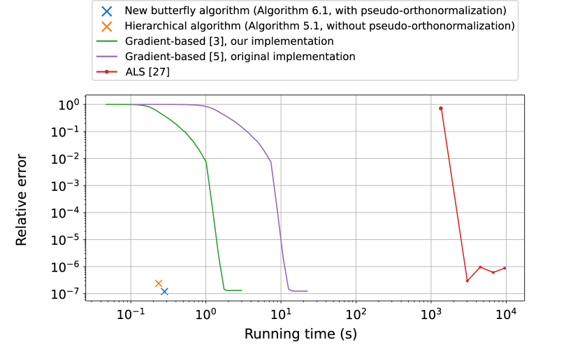
Figure 3: Relative approximation errors defined as $\|\mathbf{A}-\hat{\mathbf{A}}\|_{F}/\|\mathbf{A}\|_{F}$ vs. running time of the different algorithms. The target matrix $\mathbf{A}$ is the Hadamard matrix of size $1024\times 1024$, and $\hat{\mathbf{A}}$ is the computed approximation for Problem (1) associated with the square dyadic butterfly architecture.

Figure 3 shows that the different methods find an approximate solution nearly up to machine precision, but hierarchical algorithms are several orders of magnitude faster than the gradient-based method [5] and ALS [27]. Using Algorithm 4 without pseudo-orthonormalization operations is also faster than with these operations. We however show the positive practical impact of pseudo-orthonormalization on noisy problems in the following section.

8.2 To orthonormalize or not to orthonormalize?

We now study in practice the impact of the pseudo-orthonormalization operations in the new butterfly algorithm, in terms of running time and approximation error, at different scales of the matrix size $n$ with $n\in\{2^{i}\mid i=7,\ldots,13\}$. We consider Problem (1) associated with a chainable architecture ${\boldsymbol{\beta}}=({\boldsymbol{\pi}}_{1},\ldots,{\boldsymbol{\pi}}_{4})$ such that:

• Each factor is of size $(a_{\ell}b_{\ell}d_{\ell},a_{\ell}c_{\ell}d_{\ell})=(n,n)$

• $\mathcal{B}^{{\boldsymbol{\beta}}}$ contains some dense matrices: ${\boldsymbol{\pi}}_{1}*{\boldsymbol{\pi}}_{2}*{\boldsymbol{\pi}}_{3}*{\boldsymbol{\pi}}_{4}=(1,n,n,1)$;

• In the complementary low-rank characterization of $\mathcal{B}^{{\boldsymbol{\beta}}}$, the rank constraint on the submatrices is $r\geq 2$, i.e., $\mathbf{r}({\boldsymbol{\beta}})=(r,r,r)$. We do not choose $r=1$ because the pseudo-orthonormalization operations would then be equivalent to some simple rescaling.

Among all of such architectures (that can be characterized and found using Lemma 4.26), we choose the one with the smallest number of parameters, i.e., yielding the smallest $\|{\boldsymbol{\beta}}\|_{0}$. The considered target matrix is $\mathbf{A}=\tilde{\mathbf{A}}+\epsilon\frac{\|\tilde{\mathbf{A}}\|_{F}}{\|\mathbf{E}\|_{F}}\mathbf{E}$, where $\tilde{\mathbf{A}}:=\mathbf{X}_{1}\mathbf{X}_{2}\mathbf{X}_{3}\mathbf{X}_{4}$, the entries of $\mathbf{X}_{\ell}\in\Sigma^{{\boldsymbol{\pi}}_{\ell}}$ for $\ell\in\llbracket 4\rrbracket$ are i.i.d. sampled from the uniform distribution in the interval $[0,1]$, $\mathbf{E}$ is an i.i.d. centered Gaussian matrix with the standard deviation $1$, and $\epsilon=0.1$ is the noise level. The permutation $\sigma$ for the butterfly algorithm is $\sigma=(2,1,3)$, which corresponds to the balanced factor-bracketing tree of $\llbracket 4\rrbracket$.

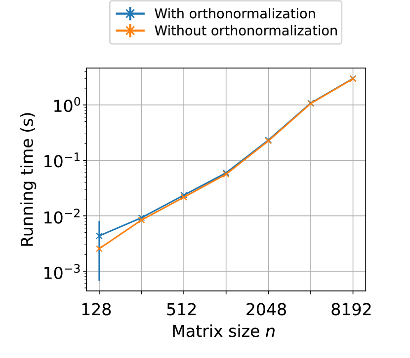
(a) Running time vs. size $n$

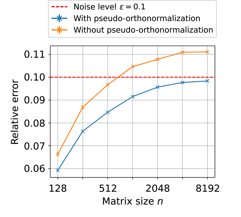
(b) Relative error $\frac{\|\mathbf{A}-\hat{\mathbf{A}}\|_{F}}{\|\mathbf{A}\|_{F}}$ vs. size $n$

Figure 4: Running time and the relative approximation errors vs. the matrix size $n$, for Algorithm 4 (with or without pseudo-orthonormalization), for the instance of Problem (1) described in Section 8.2 with $L=4$, $r=4$. We show mean and standard deviation on the error bars over $10$ repetitions of the experiment.

Figure 4(a) shows that the difference in running time between the new butterfly algorithm (Algorithm 4) with and without pseudo-orthonormalization is negligible, in the regime of large matrix size $n\geq 512$. This means that, asymptotically, the time of orthonormalization operations is not the bottleneck, which is coherent with our complexity analysis given in Theorem 6.5.

In terms of the approximation error, Figure 4(b) shows that the hierarchical algorithm (Algorithm 4) with pseudo-orthonormalization returns a smaller (i.e., better) approximation error. Moreover, the relative error with pseudo-orthonormalization error is always smaller than the relative noise level $\epsilon=0.1$ (cf. Figure 8 for other values of $\epsilon$), which is not the case for the hierarchical algorithm without pseudo-orthonormalization (Algorithm 3). In conclusion, besides yielding error guarantees of the form (3), the pseudo-orthonormalization operations in our experiments also lead to better approximation in practice.

8.3 Numerical assessment of the bounds

In this section, we numerically evaluate the bounds given by Theorem 7.2 and Theorem 7.3. The setting is identical to that of the previous section, except that:

1. We run the new butterfly algorithm (Algorithm 4) with multiple permutations associated to various factor-bracketing trees: identity permutation (left-to-right tree, cf. Example 5.4 or [44]), balance permutation (corresponding to the so-called “balanced tree” [44]) and a random one.

2. The number of factors is $L=5$. The size of the matrix is $4608$. The number $4608=3^{2}\times 2^{9}$ is a common matrix size appearing when one replaces convolutional layers by a product of butterfly factors [27] (the factor $3^{2}$ corresponds to a convolutional kernel of size $3\times 3$). This matrix size is non-dyadic, which partly illustrates the versatility of butterfly factors in replacing linear operators.

3. The experiments are repeated $10$ times. The plots in Fig. 5 show the average and standard deviation values of the relative error and of the bounds. The standard deviations are not visible due to their small size and the log scale of the plot.

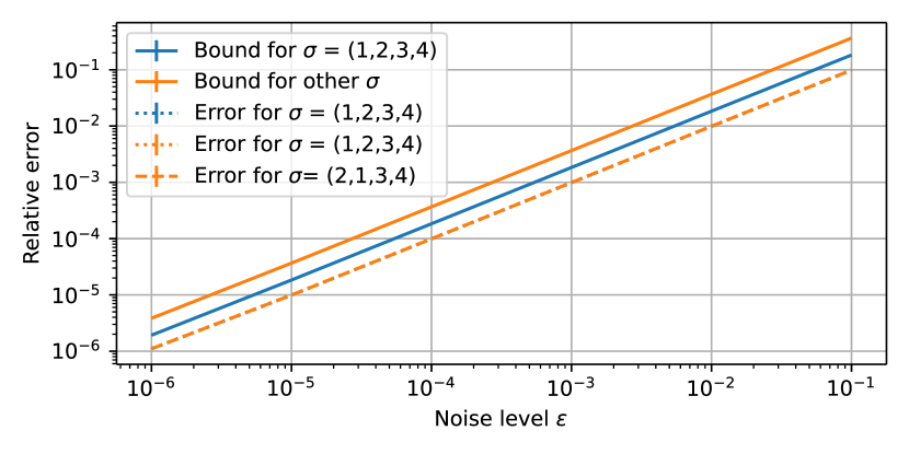
Figure 5: Bounds and numerical errors of Algorithm 4 with different permutations (associated to different factor bracketing trees): identity permutation $(1,2,3,4)$, “balanced” permutation $(2,1,3,4)$, randomized permutation ($(4,1,2,3)$ in this experiment). The bound for the identity permutation is given by Theorem 7.3 while the others are given by Theorem 7.2. Vertical bars show standard deviations over 10 experiments, but they are not visible on the graph because they are small. Note that all error curves (discontinuous lines) are overlapping, so we are seeing only one of them.

We report the relative errors and the bounds corresponding to each permutation in Fig. 5. It is well illustrated by Fig. 5 that our theoretical results in Theorem 7.2 and Theorem 7.3 are correct. The bound in Theorem 7.3 (Fig. 5-a) is visibly tighter than the one in Theorem 7.2 (Fig. 5-b,c) although there is no significant difference among the errors obtained by the three permutations corresponding to different factor bracketing trees (the errors for the three different permutations are almost identical, which makes only one error plot visible).

9 Conclusion

We proposed a general definition of (deformable) butterfly architectures, together with a new butterfly algorithm for the problem of (deformable) butterfly factorization (1), endowed with new guarantees on the approximation error of the type (3), under the condition that the associated architecture ${\boldsymbol{\beta}}$ satisfies a so-called chainability condition. The proposed algorithm involves some novel orthonormalization operations in the context of butterfly factorization. We discuss some perspectives of this work.

Tightness of the error bound. The constants $C_{\boldsymbol{\beta}}$ in Theorem 7.4 scale linearly or even sub-linearly with respect to the depth $L=|{\boldsymbol{\beta}}|$ of the architecture. Note that the quasi-linear constant $C_{n}$ in the existing bound (33) is not comparable with the constants $C_{\boldsymbol{\beta}}$ in Theorem 7.4, due to the presence of $\epsilon_{0}$ in the bound (33), whereas the constants $C_{\boldsymbol{\beta}}$ in Theorem 7.4 controls the ratio between the approximation error and the minimal error. A natural question is whether the constants $C_{\boldsymbol{\beta}}$ in Theorem 7.4 are tight for an error bound of the type (3). If not, can the bounds for the proposed be algorithm be sharpened by a refined theoretical analysis, or is there another algorithm that yields a smaller constant $C_{\boldsymbol{\beta}}$ in the error bound?

Randomized algorithms for low-rank approximation. Algorithms 3 and 4 need to access all the elements of the target matrix $\mathbf{A}\in\mathbb{C}^{m\times n}$. Thus, the complexity of all algorithms is at least $\mathcal{O}(mn)$. This complexity, however, fails to scale for large $m,n$ (e.g., up to $10^{6}$). Assuming that the target matrix admits a butterfly factorization associated with ${\boldsymbol{\beta}}$, i.e., $\mathbf{A}\in\mathcal{B}^{{\boldsymbol{\beta}}}$, is it possible to recover the butterfly factors of $\mathbf{A}$, with a faster algorithm, ideally of complexity $\mathcal{O}(\|{\boldsymbol{\beta}}\|_{0})$? Note that this question was already considered in [23, 22] where randomized algorithms for low-rank approximation [16, 26] are leveraged in the context of butterfly factorization. The question is therefore whether we can still prove some theoretical guarantees of the form (3) for butterfly algorithms with such algorithms.

Algorithms beyond the chainability assumption. Although chainability is a sufficient condition for which we can design an algorithm with guarantees on the approximation error, it is natural to ask whether it is also a necessary condition. There exist, in fact, non-chainable architectures for which we can still build an algorithm yielding an error bound (3). For instance, this is the case of arbitrary architectures of depth $L=2$ (see Lemma 5.1); or of architectures that satisfy a transposed version of Definition 4.11: such architectures can easily be checked to cover some non-chainable architectures, and Algorithm 4 can be easily adapted to have guarantees similar to Theorems 7.2 and 7.3. Therefore, chainability in the sense of Definition 4.11 is not necessary for theoretical guarantees of the form (3). Whether algorithms with performance guarantees can be derived beyond the three above-mentioned cases remains open.

Efficient implementation of butterfly matrix multiplication. While the complexity of matrix-vector multiplication by a $n\times m$ butterfly matrix associated with ${\boldsymbol{\beta}}$ is theoretically subquadratic if $\|{\boldsymbol{\beta}}\|_{0}=o(mn)$, a practical fast implementation of such a matrix multiplication is not straightforward [13], since dense matrix multiplication algorithms are competitive, e.g., on GPUs. Future work can focus on efficient implementations of butterfly matrix multiplication on different kinds of hardware, in order to harness all of the benefits of the butterfly structure for large-scale applications, like in machine learning for instance.

Butterfly factorization with unknown permutations. In general, it is necessary to take into account row and column permutations in the butterfly factorization problem for more flexibility of the butterfly model $\Sigma^{{\boldsymbol{\beta}}}$ for an architecture ${\boldsymbol{\beta}}$. For instance, as mentioned above, the DFT matrix admits a square dyadic butterfly factorization up to the bit-reversal permutation of column indices. Therefore, as in [43], the general approximation problem that takes into account row and column permutations is:

(34) $$\inf_{({\mathbf{X}}_{\ell})_{\ell=1}^{L}\in\Sigma^{{\boldsymbol{\beta}}},\mathbf{P},\mathbf{Q}}\|\mathbf{A}-\mathbf{Q}^{\top}{\mathbf{X}}_{1}\ldots{\mathbf{X}}_{L}\mathbf{P}\|_{F},$$

where $\mathbf{P}$, $\mathbf{Q}$ are unknown permutations part of the optimization problem. Without any further assumption on the target matrix $\mathbf{A}$, solving this approximation problem is conjectured to be difficult. Future work can further study this more general problem, based on the existing heuristic proposed in [43].

Appendix A Proof for results in Section 3

This section is devoted to the proof of Theorem 3.4. To that end we first introduce the following technical lemma.

Lemma A.1.

Consider support constraints $\mathbf{L}\in\{0,1\}^{m\times s}$, $\mathbf{R}\in\{0,1\}^{r\times n}$ satisfying the conditions of Theorem 3.4. With the notations $R_{P}\subseteq\llbracket m\rrbracket$, $C_{P}\subseteq\llbracket n\rrbracket$, $\mathcal{P}[\mathbf{L},\mathbf{R}]$ from Definition 3.3, for each $(\mathbf{X},\mathbf{Y})$ such that $\mathtt{supp}(\mathbf{X})\subseteq\mathbf{L},\mathtt{supp}(\mathbf{Y})\subseteq\mathbf{R}$, we have:

(35) $$\forall P\in\mathcal{P}(\mathbf{L},\mathbf{R}),\quad(\mathbf{X}\mathbf{Y})[R_{P},C_{P}]=\mathbf{X}[R_{P},P]\mathbf{Y}[P,C_{P}].$$

Proof A.2.

For any pair of matrices $(\mathbf{X},\mathbf{Y})\in\mathbb{C}^{m\times r}\times\mathbb{C}^{r\times n}$:

(36) $$\mathbf{X}\mathbf{Y}=\sum_{i=1}^{r}\mathbf{X}[{:,{i}}]\mathbf{Y}[{{i},:}]=\sum_{P\in\mathcal{P}(\mathbf{L},\mathbf{R})}\mathbf{X}[{:,{P}}]\mathbf{Y}[{{P},:}].$$

For $P,\tilde{P}\in\mathcal{P}(\mathbf{L},\mathbf{R})$ with $P\neq\tilde{P}$, the components $\mathbf{U}_{P}$ and $\mathbf{U}_{\tilde{P}}$ of Definition 3.3 are disjoint by assumption on $\mathbf{L},\mathbf{R}$. Since $\mathtt{supp}(\mathbf{X}[{:,{\tilde{P}}}]\mathbf{Y}[{{\tilde{P}},:}])\subseteq\mathbf{U}_{\tilde{P}}$, we have $(\mathbf{X}[{:,{\tilde{P}}}]\mathbf{Y}[{{\tilde{P}},:}])[R_{P},C_{P}]=\mathbf{0}$, and by (36) it follows that we have $(\mathbf{X}\mathbf{Y})[R_{P},C_{P}]=(\mathbf{X}[{:,{P}}]\mathbf{Y}[{{P},:}])[R_{P},C_{P}]=\mathbf{X}[R_{P},P]\mathbf{Y}[P,C_{P}].$

The following proof of Theorem 3.4 is mainly taken from [18], but we additionally compute the infimum value of Problem (4).

Proof A.3 (Proof for Theorem 3.4).

We use the shorthand $\mathcal{P}$ for $\mathcal{P}(\mathbf{L},\mathbf{R})$, and denote $\Sigma:=\{(\mathbf{X},\mathbf{Y})\,|\,\mathtt{supp}(\mathbf{X})\subseteq\mathbf{L},\,\mathtt{supp}(\mathbf{Y})\subseteq\mathbf{R}\}$. Recall that $({\mathbf{U}}_{i})_{i=1}^{r}:=\varphi(\mathbf{X},\mathbf{Y})$ with $\varphi$ from Definition 3.1. Let $(\mathbf{X},\mathbf{Y})\in\Sigma$. Then, $\mathtt{supp}(\mathbf{X}[{:,{P}}]\mathbf{Y}[{{P},:}])\subseteq\mathbf{U}_{P}$ for any $P\in\mathcal{P}$, hence $\mathtt{supp}(\mathbf{X}\mathbf{Y})\subseteq\bigcup_{P\in\mathcal{P}}\mathbf{U}_{P}$, and $(\mathbf{X}\mathbf{Y})\odot\overline{\mathbf{U}_{\mathcal{P}}}=\mathbf{0}$ where we denote $\overline{\mathbf{U}_{\mathcal{P}}}:=(\llbracket m\rrbracket\times\llbracket n\rrbracket)\setminus\left(\bigcup_{P\in\mathcal{P}}\mathbf{U}_{P}\right)$. Moreover, by assumption, $\mathbf{U}_{P}$ and $\mathbf{U}_{\tilde{P}}$ are disjoint for any $P,\tilde{P}\in\mathcal{P}$ such that $P\neq\tilde{P}$, so:

(37) $$\begin{split}\|\mathbf{A}-\mathbf{X}\mathbf{Y}\|_{F}^{2}&=\left(\sum_{P\in\mathcal{P}}\|(\mathbf{A}-\mathbf{X}\mathbf{Y})\odot\mathbf{U}_{P}\|_{F}^{2}\right)+\|(\mathbf{A}-\mathbf{X}\mathbf{Y})\odot\overline{\mathbf{U}_{\mathcal{P}}}\|_{F}^{2}\\ &=\left(\sum_{P\in\mathcal{P}}\|(\mathbf{A}-\mathbf{X}\mathbf{Y})[R_{P},C_{P}]\|_{F}^{2}\right)+\|\mathbf{A}\odot\overline{\mathbf{U}_{\mathcal{P}}}\|_{F}^{2}\\ &=\left(\sum_{P\in\mathcal{P}}\|{\mathbf{A}}[R_{P},C_{P}]-{(\mathbf{X}\mathbf{Y})}[R_{P},C_{P}]\|_{F}^{2}\right)+\|\mathbf{A}\odot\overline{\mathbf{U}_{\mathcal{P}}}\|_{F}^{2}\\ &\overset{\eqref{eq:submatrixequality}}{=}\left(\sum_{P\in\mathcal{P}}\|{\mathbf{A}}[R_{P},C_{P}]-{\mathbf{X}}[R_{P},P]{\mathbf{Y}}[P,C_{P}]\|_{F}^{2}\right)+\|\mathbf{A}\odot\overline{\mathbf{U}_{\mathcal{P}}}\|_{F}^{2}.\end{split}$$

Since $\mathcal{P}$ is a partition, this implies that each term in the sum $\sum_{P\in\mathcal{P}}\|{\mathbf{A}}[R_{P},C_{P}]-{\mathbf{X}}[R_{P},P]{\mathbf{Y}}[P,C_{P}]\|^{2}$ involves columns of $\mathbf{X}$ and rows of $\mathbf{Y}$ that are not involved in other terms of the sum. Moreover, we remark that for any $P\in\mathcal{P}$, the matrix ${\mathbf{X}}[R_{P},P]{\mathbf{Y}}[P,C_{P}]$ is of rank at most $|P|$. In other words, minimizing the right-hand-side of (37) with respect to $(\mathbf{X},\mathbf{Y})\in\Sigma$ is equivalent to minimize each term of the sum for $P\in\mathcal{P}$, which is the problem of finding the best rank-$|P|$ approximation of ${\mathbf{A}}[R_{P},C_{P}]$. This yields the claimed equation (5).

Appendix B Proof for results in Section 4 and Section 5.1

B.1 Proof of Proposition 4.8

Proof B.1.

Let $r=r({\boldsymbol{\pi}}_{1},{\boldsymbol{\pi}}_{2})$. By Definition 4.6, $a_{1}\mid a_{2}$ and $d_{2}\mid d_{1}$, so there are two integers $q,s$ such that $a_{2}=qa_{1}$ and $d_{1}=sd_{2}$. Since $a_{1}c_{1}/a_{2}=b_{2}d_{2}/d_{1}=r$ by Definition 4.6, this yields $c_{1}=a_{2}r/a_{1}=rq$, $b_{2}=d_{1}r/d_{2}=rs$. Thus,

$$\mathbf{S}_{{\boldsymbol{\pi}}_{1}}\mathbf{S}_{{\boldsymbol{\pi}}_{2}} =\left(\mathbf{I}_{a_{1}}\otimes\mathbf{1}_{b_{1}\times rq}\otimes\mathbf{I}_{d_{1}}\right)\left(\mathbf{I}_{a_{2}}\otimes\mathbf{1}_{rs\times c_{2}}\otimes\mathbf{I}_{d_{2}}\right)$$

$$=\left(\mathbf{I}_{a_{1}}\otimes\mathbf{1}_{b_{1}\times q}\otimes\mathbf{1}_{1\times r}\otimes\mathbf{I}_{d_{1}}\right)\left(\mathbf{I}_{a_{2}}\otimes\mathbf{1}_{r\times 1}\otimes\mathbf{1}_{s\times c_{2}}\otimes\mathbf{I}_{d_{2}}\right)$$

$$=\left[(\mathbf{I}_{a_{1}}\otimes\mathbf{1}_{b_{1}\times q})\otimes\mathbf{1}_{1\times r}\otimes\mathbf{I}_{d_{1}}\right]\left[\mathbf{I}_{a_{2}}\otimes\mathbf{1}_{r\times 1}\otimes(\mathbf{1}_{s\times c_{2}}\otimes\mathbf{I}_{d_{2}})\right]$$

$$\overset{(\star)}{=}\left(\mathbf{I}_{a_{1}}\otimes\mathbf{1}_{b_{1}\times q}\right)\otimes\left(\mathbf{1}_{1\times r}\mathbf{1}_{r\times 1}\right)\otimes\left(\mathbf{1}_{s\times c_{2}}\otimes\mathbf{I}_{d_{2}}\right)$$

$$=\left(\mathbf{I}_{a_{1}}\otimes\mathbf{1}_{b_{1}\times q}\right)\otimes\left(r\mathbf{1}_{1\times 1}\right)\otimes\left(\mathbf{1}_{s\times c_{2}}\otimes\mathbf{I}_{d_{2}}\right)$$

$$=r\left(\mathbf{I}_{a_{1}}\otimes\mathbf{1}_{b_{1}s\times qc_{2}}\otimes\mathbf{I}_{d_{2}}\right)$$

$$=r\mathbf{S}_{{\boldsymbol{\pi}}_{1}*{\boldsymbol{\pi}}_{2}}\quad\left(\text{because }\frac{b_{1}d_{1}}{d_{2}}=b_{1}s\text{ and }\frac{a_{2}c_{2}}{c_{1}}=qc_{2}\right).$$

We can use the equality $(\mathbf{A}\otimes\mathbf{C}\otimes\mathbf{E})(\mathbf{B}\otimes\mathbf{D}\otimes\mathbf{F})=(\mathbf{AB})\otimes(\mathbf{CD})\otimes(\mathbf{E}\mathbf{F})$ in $(\star)$ because, according to our conditions for chainability, the sizes of $\mathbf{A},\mathbf{B},\mathbf{C},\mathbf{D},\mathbf{E},\mathbf{F}$ in $(\star)$ make the matrix products $\mathbf{AB},\mathbf{C}\mathbf{D}$ and $\mathbf{EF}$ well-defined.

B.2 Proof of Lemma 4.9

We prove the claims in Lemma 4.9 one by one.

1. Follows by the definition of $R_{P}$ and $C_{P}$.

2. It can be easily verified that the column supports $\{{\mathbf{S}_{{\boldsymbol{\pi}}_{1}}}[:,j]\}_{j}$ (resp. the row supports $\{{\mathbf{S}_{{\boldsymbol{\pi}}_{2}}}[i,:]\}_{i}$) are pairwise disjoint or identical, due to the support structure of the form $\mathbf{I}_{a}\otimes\mathbf{1}_{b\times c}\otimes\mathbf{I}_{d}$ of a Kronecker-sparse factor. Indeed, the columns (resp. rows) of the Kronecker product $\mathbf{A}\otimes\mathbf{B}$ are equal to the Kronecker product of columns and rows of $\mathbf{A}$ and $\mathbf{B}$ and the matrices $\mathbf{A},\mathbf{B}$ appearing in our case are either identity matrices or all-one matrices. Thus, for each $P\in\mathcal{P}(\mathbf{S}_{{\boldsymbol{\pi}}_{1}},\mathbf{S}_{{\boldsymbol{\pi}}_{2}})$ the sets $R_{P}\times C_{P}={\mathbf{S}_{{\boldsymbol{\pi}}_{1}}}[:,i]\times{\mathbf{S}_{{\boldsymbol{\pi}}_{2}}}[i,:]$ are pairwise disjoint.

3. For any $P\in\mathcal{P}(\mathbf{S}_{{\boldsymbol{\pi}}_{1}},\mathbf{S}_{{\boldsymbol{\pi}}_{2}})$, by Definition 4.1 we have $|R_{P}|=b_{1},|C_{P}|=c_{2}$. Setting $r:=r({\boldsymbol{\pi}}_{1},{\boldsymbol{\pi}}_{2})$, we have

   $$\sum_{P\in\mathcal{P}(\mathbf{S}_{{\boldsymbol{\pi}}_{1}},\mathbf{S}_{{\boldsymbol{\pi}}_{2}})}|P|\,\mathbf{U}_{P}\stackrel{{\scriptstyle\textrm{Def. \ref{def:classequivalence}}}}{{=}}\sum_{\mathbf{U}_{i}\in\varphi(\mathbf{S}_{{\boldsymbol{\pi}}_{1}},\mathbf{S}_{{\boldsymbol{\pi}}_{2}})}\mathbf{U}_{i}=\mathbf{S}_{{\boldsymbol{\pi}}_{1}}\mathbf{S}_{{\boldsymbol{\pi}}_{2}}\stackrel{{\scriptstyle\textrm{Prop. \ref{prop:stability}}}}{{=}}r\mathbf{S}_{({\boldsymbol{\pi}}_{1}*{\boldsymbol{\pi}}_{2})},$$

   where the second equality simply comes from the rank-one decomposition of matrix multiplication. Since all $\mathbf{U}_{P}$’s have pairwise disjoint supports (from point 2), we get $|P|=r$ for each $P\in\mathcal{P}(\mathbf{S}_{{\boldsymbol{\pi}}_{1}},\mathbf{S}_{{\boldsymbol{\pi}}_{2}})$.

4. $\mathtt{supp}(\mathbf{S}_{{\boldsymbol{\pi}}_{1}*{\boldsymbol{\pi}}_{2}})=\mathtt{supp}(\mathbf{S}_{{\boldsymbol{\pi}}_{1}}\mathbf{S}_{{\boldsymbol{\pi}}_{2}})$ is a consequence of Proposition 4.8. The second equality, $\mathtt{supp}(\mathbf{S}_{{\boldsymbol{\pi}}_{1}}\mathbf{S}_{{\boldsymbol{\pi}}_{2}})=\cup_{P\in\mathcal{P}}R_{P}\times C_{P}$, is a consequence of the rank-one decomposition of the matrix multiplication, i.e., $\mathbf{X}\mathbf{Y}=\sum_{i}\mathbf{X}[{:,{i}}]\mathbf{Y}[{{i},:}]$, and of the fact that $\mathbf{S}_{{\boldsymbol{\pi}}_{1}},\mathbf{S}_{{\boldsymbol{\pi}}_{2}}$ have non-negative coefficients (thus, the support is equal to the union, and it is not just a subset).

B.3 Proof for Lemma 4.10

Denote ${\boldsymbol{\pi}}_{\ell}=(a_{\ell},b_{\ell},c_{\ell},d_{\ell})$ for $\ell\in\llbracket 3\rrbracket$. Let us show that ${\boldsymbol{\pi}}_{1}$ and ${\boldsymbol{\pi}}_{2}*{\boldsymbol{\pi}}_{3}$ are chainable and $r({\boldsymbol{\pi}}_{1},{\boldsymbol{\pi}}_{2}*{\boldsymbol{\pi}}_{3})=r({\boldsymbol{\pi}}_{1},{\boldsymbol{\pi}}_{2})$. Since $({\boldsymbol{\pi}}_{2},{\boldsymbol{\pi}}_{3})$ is chainable, by definition of $*$ (Definition 4.6), we have:

$$(\tilde{a},\tilde{b},\tilde{c},\tilde{d})={\tilde{{\boldsymbol{\pi}}}}:={\boldsymbol{\pi}}_{2}*{\boldsymbol{\pi}}_{3}=\left(a_{2},\frac{b_{2}d_{2}}{d_{3}},\frac{a_{3}c_{3}}{a_{2}},d_{3}\right).$$

We then verify that $({\boldsymbol{\pi}}_{1},{\tilde{{\boldsymbol{\pi}}}})$ satisfies the conditions of Definition 4.6:

1. By chainability of $({\boldsymbol{\pi}}_{1},{\boldsymbol{\pi}}_{2})$, we have $r({\boldsymbol{\pi}}_{1},{\boldsymbol{\pi}}_{2}):=a_{1}c_{1}/a_{2}=b_{2}d_{2}/d_{1}\in\mathbb{N}$. Therefore: $a_{1}c_{1}/\tilde{a}=a_{1}c_{1}/a_{2}=r({\boldsymbol{\pi}}_{1},{\boldsymbol{\pi}}_{2})=b_{2}d_{2}/d_{1}=\tilde{b}\tilde{d}/d_{1}\in\mathbb{N}$. This means that $r({\boldsymbol{\pi}}_{1},{\boldsymbol{\pi}}_{2}*{\boldsymbol{\pi}}_{3})=r({\boldsymbol{\pi}}_{1},{\boldsymbol{\pi}}_{2})$.

2. By chainability of $({\boldsymbol{\pi}}_{1},{\boldsymbol{\pi}}_{2})$, we have $a_{1}\mid a_{2}=\tilde{a}$.

3. By chainability of $({\boldsymbol{\pi}}_{2},{\boldsymbol{\pi}}_{3})$ (resp. of $({\boldsymbol{\pi}}_{1},{\boldsymbol{\pi}}_{2})$) we have $\tilde{d}=d_{3}\mid d_{2}\mid d_{1}$.

In conclusion, $({\boldsymbol{\pi}}_{1},{\boldsymbol{\pi}}_{2}*{\boldsymbol{\pi}}_{3})$ is chainable with $r({\boldsymbol{\pi}}_{1},{\boldsymbol{\pi}}_{2}*{\boldsymbol{\pi}}_{3})=r({\boldsymbol{\pi}}_{1},{\boldsymbol{\pi}}_{2})$. Computing ${\boldsymbol{\pi}}_{1}*({\boldsymbol{\pi}}_{2}*{\boldsymbol{\pi}}_{3})$ explicitly by (9) gives ${\boldsymbol{\pi}}_{1}*({\boldsymbol{\pi}}_{2}*{\boldsymbol{\pi}}_{3})=\left(a_{1},\frac{b_{1}d_{1}}{d_{3}},\frac{a_{3}c_{3}}{a_{1}},d_{3}\right)$. Similarly, we can show that $({\boldsymbol{\pi}}_{1}*{\boldsymbol{\pi}}_{2},{\boldsymbol{\pi}}_{3})$ is also chainable with $r({\boldsymbol{\pi}}_{1}*{\boldsymbol{\pi}}_{2},{\boldsymbol{\pi}}_{3})=r({\boldsymbol{\pi}}_{2},{\boldsymbol{\pi}}_{3})$, and we can indeed verify that $({\boldsymbol{\pi}}_{1}*{\boldsymbol{\pi}}_{2})*{\boldsymbol{\pi}}_{3}={\boldsymbol{\pi}}_{1}*({\boldsymbol{\pi}}_{2}*{\boldsymbol{\pi}}_{3})$ using (9).

B.4 Proof of Lemma 4.13 - explicit formula for $({\boldsymbol{\pi}}_{1}*\ldots*{\boldsymbol{\pi}}_{L})$ in (11)

We show that ${\boldsymbol{\pi}}_{1}*\ldots*{\boldsymbol{\pi}}_{L}=\left(a_{1},\frac{b_{1}d_{1}}{d_{L}},\frac{a_{L}c_{L}}{a_{1}},d_{L}\right)$, for each chainable architecture ${\boldsymbol{\beta}}=({\boldsymbol{\pi}}_{\ell})_{\ell=1}^{L}=(a_{\ell},b_{\ell},c_{\ell},d_{\ell})_{\ell=1}^{L}$ of depth $L\geq 2$. The proof is an induction on $L\geq 2$. If $L=2$, the result comes from (9). Let $L\geq 2$, and assume that the statement holds for any chainable architecture of depth $L$. Consider a chainable architecture ${\boldsymbol{\beta}}:=({\boldsymbol{\pi}}_{\ell})_{\ell=1}^{L+1}=(a_{\ell},b_{\ell},c_{\ell},d_{\ell})_{\ell=1}^{L+1}$ of depth $L+1$. By the induction hypothesis, we have ${\boldsymbol{\pi}}_{1}*\ldots*{\boldsymbol{\pi}}_{L}=\left(a_{1},\frac{b_{1}d_{1}}{d_{L}},\frac{a_{L}c_{L}}{a_{1}},d_{L}\right)$. Therefore,

$${\boldsymbol{\pi}}_{1}*\ldots*{\boldsymbol{\pi}}_{L}*{\boldsymbol{\pi}}_{L+1} =\left(a_{1},\frac{b_{1}d_{1}}{d_{L}},\frac{a_{L}c_{L}}{a_{1}},d_{L}\right)*(a_{L+1},b_{L+1},c_{L+1},d_{L+1})$$

$$=\left(a_{1},\frac{b_{1}d_{1}d_{L}}{d_{L}d_{L+1}},\frac{a_{L+1}c_{L+1}}{a_{1}},d_{L+1}\right)$$

$$=\left(a_{1},\frac{b_{1}d_{1}}{d_{L+1}},\frac{a_{L+1}c_{L+1}}{a_{1}},d_{L+1}\right).$$

B.5 Proof for Lemma 4.16

By (11), we have:

(38) $$(a,b,c,d) ={\boldsymbol{\pi}}:={\boldsymbol{\pi}}_{q}*\ldots*{\boldsymbol{\pi}}_{s}=\left(a_{q},\frac{b_{q}d_{q}}{d_{s}},\frac{a_{s}c_{s}}{a_{q}},d_{s}\right),$$

$$(a^{\prime},b^{\prime},c^{\prime},d^{\prime}) ={\boldsymbol{\pi}}^{\prime}:={\boldsymbol{\pi}}_{s+1}*\ldots*{\boldsymbol{\pi}}_{t}=\left(a_{s+1},\frac{b_{s+1}d_{s+1}}{d_{t}},\frac{a_{t}c_{t}}{a_{s+1}},d_{t}\right).$$

We show the chainability of $({\boldsymbol{\pi}},{\boldsymbol{\pi}}^{\prime})$ by verifying the conditions of Definition 4.6:

1. By chainability of $({\boldsymbol{\pi}}_{s},{\boldsymbol{\pi}}_{s+1})$, $r({\boldsymbol{\pi}}_{s},{\boldsymbol{\pi}}_{s+1})=a_{s}c_{s}/a_{s+1}=b_{s+1}d_{s+1}/d_{s}\in\mathbb{N}$. This means that $ac/a^{\prime}=a_{s}c_{s}/a_{s+1}=r({\boldsymbol{\pi}}_{s},{\boldsymbol{\pi}}_{s+1})=b_{s+1}d_{s+1}/d_{s}=b^{\prime}d^{\prime}/d$ and $r({\boldsymbol{\pi}},{\boldsymbol{\pi}}^{\prime})=r({\boldsymbol{\pi}}_{s},{\boldsymbol{\pi}}_{s+1})\in\mathbb{N}$.

2. By chainability of ${\boldsymbol{\beta}}$, $a_{\ell}\mid a_{\ell+1}$ for $\ell\in\llbracket L-1\rrbracket$, so $a=a_{q}\mid a_{s+1}=a^{\prime}$ since $q\leq s$.

3. Similarly $d_{\ell+1}\mid d_{\ell}$ for all $\ell\in\llbracket L-1\rrbracket$, so $d^{\prime}=d_{t}\mid d_{s}=d$

B.6 Proof for Lemma 4.19

The explicit formulas for $(a,b,c,d)={\boldsymbol{\pi}}:={\boldsymbol{\pi}}_{q}*\ldots*{\boldsymbol{\pi}}_{s}$ and $(a^{\prime},b^{\prime},c^{\prime},d^{\prime})={\boldsymbol{\pi}}^{\prime}:={\boldsymbol{\pi}}_{s+1}*\ldots*{\boldsymbol{\pi}}_{t}$ are given in (38). By Lemma 4.16, $({\boldsymbol{\pi}},{\boldsymbol{\pi}}^{\prime})$ is chainable, with $r({\boldsymbol{\pi}},{\boldsymbol{\pi}}^{\prime})=r({\boldsymbol{\pi}}_{s},{\boldsymbol{\pi}}_{s+1})$. To show the non-redundancy of $({\boldsymbol{\pi}},{\boldsymbol{\pi}}^{\prime})$, it remains to show $r({\boldsymbol{\pi}},{\boldsymbol{\pi}}^{\prime})<\min(b,c^{\prime})$. Let us show $r({\boldsymbol{\pi}},{\boldsymbol{\pi}}^{\prime})<b$. Because ${\boldsymbol{\beta}}$ is not redundant, by Definition 4.17, we have $r({\boldsymbol{\pi}}_{\ell},{\boldsymbol{\pi}}_{\ell+1})<b_{\ell}$ for any $\ell\in\llbracket L-1\rrbracket$. But $r({\boldsymbol{\pi}}_{\ell},{\boldsymbol{\pi}}_{\ell+1})=b_{\ell+1}d_{\ell+1}/d_{\ell}$ by Definition 4.6. Therefore, $b_{\ell+1}d_{\ell+1}<b_{\ell}d_{\ell}$ for any $\ell\in\llbracket L-1\rrbracket$. Thus, since $q\leq s$, we have $b_{s+1}d_{s+1}<b_{q}d_{q}$. A fortiori, $\frac{b_{s+1}d_{s+1}}{d_{s}}<\frac{b_{q}d_{q}}{d_{s}}$. But by (38), $\frac{b_{q}d_{q}}{d_{s}}=b$ and $\frac{b_{s+1}d_{s+1}}{d_{s}}=\frac{b^{\prime}d^{\prime}}{d}=r({\boldsymbol{\pi}},{\boldsymbol{\pi}}^{\prime})$. In conclusion, $r({\boldsymbol{\pi}},{\boldsymbol{\pi}}^{\prime})=\frac{b_{s+1}d_{s+1}}{d_{s}}<\frac{b_{q}d_{q}}{d_{s}}=b$. A similar argument yields $r({\boldsymbol{\pi}},{\boldsymbol{\pi}}^{\prime})<c^{\prime}$. This ends the proof.

B.7 Proof of Lemma 4.21

We first show that $(\mathbf{S}_{{\boldsymbol{\pi}}_{1}},\mathbf{S}_{{\boldsymbol{\pi}}_{2}})$ satisfies the condition of Theorem 3.4. As in the proof of point 2 of Lemma 4.9 the column supports $\{{\mathbf{S}_{{\boldsymbol{\pi}}_{1}}}[:,j]\}_{j}$ (resp. the row supports $\{{\mathbf{S}_{{\boldsymbol{\pi}}_{2}}}[i,:]\}_{i}$) are pairwise disjoint or identical, hence the components $\mathbf{U}_{i}$ of $\varphi(\mathbf{S}_{{\boldsymbol{\pi}}_{1}},\mathbf{S}_{{\boldsymbol{\pi}}_{2}})$ are pairwise disjoint or identical (if their column and row supports coincide).

Therefore, for any matrix $\mathbf{A}$, we have $\mathbf{A}\in\mathcal{B}^{{\boldsymbol{\beta}}}$ if, and only if:

$$\begin{split}&\min_{(\mathbf{X},\mathbf{Y})\in\Sigma^{{\boldsymbol{\beta}}}}\|\mathbf{A}-\mathbf{X}\mathbf{Y}\|_{F}^{2}=0\\ \overset{\eqref{eq:explicit-formula-fsmf}}{\iff}&\sum_{P\in\mathcal{P}(\mathbf{S}_{{\boldsymbol{\pi}}_{1}},\mathbf{S}_{{\boldsymbol{\pi}}_{2}})}\min_{\mathbf{B},\mathtt{rank}(\mathbf{B})\leq|P|}\|\mathbf{A}[R_{P},C_{P}]-\mathbf{B}\|_{F}^{2}+\sum_{(i,j)\notin\mathtt{supp}(\mathbf{S}_{{\boldsymbol{\pi}}_{1}}\mathbf{S}_{{\boldsymbol{\pi}}_{2}})}\mathbf{A}[i,j]^{2}=0\\ \overset{\eqref{eq:DB-support}}{\iff}&\sum_{P\in\mathcal{P}(\mathbf{S}_{{\boldsymbol{\pi}}_{1}},\mathbf{S}_{{\boldsymbol{\pi}}_{2}})}\min_{\mathbf{B},\mathtt{rank}(\mathbf{B})\leq|P|}\|\mathbf{A}[R_{P},C_{P}]-\mathbf{B}\|_{F}^{2}+\sum_{(i,j)\notin\mathtt{supp}(\mathbf{S}_{{\boldsymbol{\pi}}_{1}*{\boldsymbol{\pi}}_{2}})}\mathbf{A}[i,j]^{2}=0\\ \iff&\begin{cases}\mathtt{rank}(\mathbf{A}[R_{P},C_{P}])\leq|P|,\quad\forall P\in\mathcal{P}(\mathbf{S}_{{\boldsymbol{\pi}}_{1}},\mathbf{S}_{{\boldsymbol{\pi}}_{2}})\\ \mathbf{A}\in\Sigma^{{\boldsymbol{\pi}}_{1}*{\boldsymbol{\pi}}_{2}}\end{cases}.\end{split}$$

This proves (13).

B.8 Proof of Lemma 4.26

By Lemma 4.13 we have ${\boldsymbol{\pi}}:={\boldsymbol{\pi}}_{1}*\ldots*{\boldsymbol{\pi}}_{L}=(a_{1},b_{1}d_{1}/d_{L},a_{L}c_{L}/a_{1},d_{L})$ and $\mathcal{B}^{{\boldsymbol{\beta}}}\subseteq\Sigma^{{\boldsymbol{\pi}}}$. Since $\mathcal{B}^{{\boldsymbol{\beta}}}$ contains some dense matrices, by Definition 4.1 we must have $a_{1}=d_{L}=1$ hence ${\boldsymbol{\pi}}=(1,b_{1}d_{1},a_{L}c_{L},1)$, and the matrices in $\Sigma^{{\boldsymbol{\pi}}}$ are of size $b_{1}d_{1}\times a_{L}c_{L}$. As a result $b_{1}d_{1}=m$ and $a_{L}c_{L}=n$, so that $a_{L}\mid n$, $d_{1}\mid m$, and $b_{1}=m/d_{1}$ and $c_{L}=n/a_{L}$. Now, by chainability (see Definition 4.6) we also have $a_{1}\mid\ldots\mid a_{L}$ and $d_{L}\mid\ldots\mid d_{1}$ and, $a_{\ell}c_{\ell}/a_{\ell+1}=b_{\ell+1}d_{\ell+1}/d_{\ell}=r({\boldsymbol{\pi}}_{\ell},{\boldsymbol{\pi}}_{\ell+1}):=r_{\ell}$ for each $\ell\in\llbracket L-1\rrbracket$.

With the convention $a_{L+1}:=n$ and $d_{0}:=m$, the quantities $p_{\ell}:=a_{\ell+1}/a_{\ell}$ and $q_{\ell}:=d_{\ell-1}/d_{\ell}$, $1\leq\ell\leq L$ are thus integers, and we have $b_{1}=m/d_{1}=d_{0}/d_{1}=q_{1}$, $c_{L}=n/a_{L}=a_{L+1}/a_{L}=p_{L}$. We obtain $m=\prod_{1}^{L}p_{\ell}$, $n=\prod_{1}^{L}q_{\ell}$, and (14). For $1\leq\ell\leq L-1$ we have

(39) $$b_{\ell+1}=\frac{d_{\ell}}{d_{\ell+1}}r_{\ell}=q_{\ell+1}r_{\ell},\quad\text{and}\ c_{\ell}=\frac{a_{\ell+1}}{a_{\ell}}r_{\ell}=p_{\ell}r_{\ell}.$$

By convention $r_{0}=r_{L}=1$, hence we also have $b_{1}=q_{1}r_{1}$ and $c_{L}=p_{L}r_{L}$, so that (15) indeed holds. Vice versa it is not difficult to check that given any such integers $p_{\ell}$, $q_{\ell}$, $r_{\ell}$ the expressions (14)-(15) yield a chainable architecture enabling the construction of $\mathbf{1}_{m\times n}$, which is a dense matrix.

We now deal with non-redundancy. By Definition 4.17, each pair ${\boldsymbol{\pi}}_{\ell},{\boldsymbol{\pi}}_{\ell+1}$, $1\leq\ell\leq L-1$ is non-redundant if, and only if, $r_{\ell}:=r({\boldsymbol{\pi}}_{\ell},{\boldsymbol{\pi}}_{\ell+1})<\min(b_{\ell},c_{\ell+1})=\min(q_{\ell}r_{\ell-1},p_{\ell+1}r_{\ell+1})$. This reads

$$\frac{r_{\ell}}{r_{\ell-1}}<q_{\ell}\quad\text{and}\ \frac{r_{\ell+1}}{r_{\ell}}>\frac{1}{p_{\ell+1}},\ 1\leq\ell\leq L-1$$

or equivalently (recall that $r_{0}=r_{L}:=1$ by definition): $r_{1}<q_{1}$, $r_{L-1}<p_{L}$, and (16).

Appendix C Pseudo-orthonormalization operations of Section 6

The goal of this section is to describe the pseudo-orthonormalization operations mentioned in the new butterfly algorithm (Algorithm 4), which involve the procedure described in Algorithm 5.

Algorithm 5 Column/row-pseudo-orthonormalization

0:  Non-redundant $({\boldsymbol{\pi}}_{1},{\boldsymbol{\pi}}_{2})$, $\mathbf{X}\in\Sigma^{{\boldsymbol{\pi}}_{1}}$, $\mathbf{Y}\in\Sigma^{{\boldsymbol{\pi}}_{2}}$, $u\in\{\texttt{column},\texttt{row}\}$

0:  $(\tilde{\mathbf{X}},\tilde{\mathbf{Y}})\in\Sigma^{{\boldsymbol{\pi}}_{1}}\times\Sigma^{{\boldsymbol{\pi}}_{2}}$ such that $\tilde{\mathbf{X}}\tilde{\mathbf{Y}}=\mathbf{X}\mathbf{Y}$

1:  $(\tilde{\mathbf{X}},\tilde{\mathbf{Y}})\leftarrow(\mathbf{0},\mathbf{0})$

2:  for $P\in\mathcal{P}(\mathbf{S}_{{\boldsymbol{\pi}}_{1}},\mathbf{S}_{{\boldsymbol{\pi}}_{2}})$ (cf. Definition 3.3) do

3:     if $u$ is column then

4:        $(\mathbf{Q},\mathbf{R})\leftarrow$ QR-decomposition of $\mathbf{X}[R_{P},P]$

5:        $\tilde{\mathbf{X}}[R_{P},P]\leftarrow\mathbf{Q}$

6:        $\tilde{\mathbf{Y}}[P,C_{P}]\leftarrow\mathbf{R}\mathbf{Y}[P,C_{P}]$

7:     else if $u$ is row then

8:        $(\mathbf{Q},\mathbf{R})\leftarrow$ QR-decomposition of $\mathbf{Y}[P,C_{P}]^{\top}$

9:        $\tilde{\mathbf{X}}[R_{P},P]\leftarrow\mathbf{X}[R_{P},P]\mathbf{R}^{\top}$

10:        $\tilde{\mathbf{Y}}[P,C_{P}]\leftarrow\mathbf{Q}^{\top}$

11:     end if

12:  end for

13:  return  $(\tilde{\mathbf{X}},\tilde{\mathbf{Y}})$

First of all, let us highlight that the orthonormalization operations are well-defined only under the non-redundancy assumption. In Algorithm 5, the input pair of patterns $({\boldsymbol{\pi}}_{1},{\boldsymbol{\pi}}_{2})$ is assumed to be chainable and non-redundant, thus by Lemma 4.9 and Definition 4.17, we have $|R_{P}|\leq|P|$ and $|C_{P}|\leq|P|$, which makes the operations at lines 5 and 10 in Algorithm 5 well-defined. In Algorithm 4, the architecture ${\boldsymbol{\beta}}$ is assumed to be non-redundant. By Lemma 4.19, this means that the pair $({\boldsymbol{\pi}}_{{I}_{k}},{\boldsymbol{\pi}}_{{I}_{k+1}})$ at line 12 or the pair $({\boldsymbol{\pi}}_{{I}_{k-1}},{\boldsymbol{\pi}}_{{I}_{k}})$ at line 15 are chainable and non-redundant. This makes the call to Algorithm 5 at these lines well-defined.

In the following, we start by providing properties of left/right-$r$-unitary matrices (cf. Definition 6.1), while the second part of this section is devoted to the proof of Lemma 6.3.

C.1 Properties of left/right-$r$-unitary factors

We introduce properties related to left/right-$r$-unitary factor from Definition 6.1.

C.1.1 Norm preservation under left and right matrix multiplication

Lemma C.1.

Consider a chainable ${\boldsymbol{\beta}}:=({\boldsymbol{\pi}}_{1},{\boldsymbol{\pi}}_{2},{\boldsymbol{\pi}}_{3})$ and $\mathbf{A}_{i}\in\Sigma^{{\boldsymbol{\pi}}_{i}}$ for $i\in\llbracket 3\rrbracket$. If $\mathbf{A}_{1}$ is left-$r({\boldsymbol{\pi}}_{1},{\boldsymbol{\pi}}_{2})$-unitary and $\mathbf{A}_{3}$ is right-$r({\boldsymbol{\pi}}_{2},{\boldsymbol{\pi}}_{3})$-unitary then:

$$\|\mathbf{A}_{1}\mathbf{A}_{2}\mathbf{A}_{3}\|_{F}=\|\mathbf{A}_{2}\|_{F}.$$

Proof C.2.

By Lemma 4.10 we have $r({\boldsymbol{\pi}}_{1},{\boldsymbol{\pi}}_{2}*{\boldsymbol{\pi}}_{3})=r({\boldsymbol{\pi}}_{1},{\boldsymbol{\pi}}_{2})$, hence

$$\|\mathbf{A}_{1}\mathbf{A}_{2}\mathbf{A}_{3}\|_{F} =\|\mathbf{A}_{2}\mathbf{A}_{3}\|_{F}\quad(\text{since }\mathbf{A}_{2}\mathbf{A}_{3}\in\Sigma^{{\boldsymbol{\pi}}_{2}*{\boldsymbol{\pi}}_{3}},r({\boldsymbol{\pi}}_{1},{\boldsymbol{\pi}}_{2}*{\boldsymbol{\pi}}_{3})=r({\boldsymbol{\pi}}_{1},{\boldsymbol{\pi}}_{2}))$$

$$=\|\mathbf{A}_{2}\|_{F}\quad(\text{by~{}\lx@cref{creftypecap~refnum}{def:q-unitary}}).$$

C.1.2 Stability under matrix multiplication

Similarly to classical orthonormal matrices, left/right-$r$-unitary factors also enjoy a form of stability under matrix multiplication, in the following sense.

Lemma C.3.

Consider a chainable pair $({\boldsymbol{\pi}}_{1},{\boldsymbol{\pi}}_{2})$ and $\mathbf{A}_{i}\in\Sigma^{{\boldsymbol{\pi}}_{i}}$ for $i\in\llbracket 2\rrbracket$.

1. If $\mathbf{A}_{1}$ is left-$r({\boldsymbol{\pi}}_{1},{\boldsymbol{\pi}}_{2})$-unitary and $\mathbf{A}_{2}$ is left-$r$-unitary for some integer $r$, then the product $\mathbf{A}_{1}\mathbf{A}_{2}\in\Sigma^{{\boldsymbol{\pi}}_{1}*{\boldsymbol{\pi}}_{2}}$ is left-$r$-unitary.

2. If $\mathbf{A}_{1}$ is right-$r$-unitary for some integer $r$ and $\mathbf{A}_{2}$ is right-$r({\boldsymbol{\pi}}_{1},{\boldsymbol{\pi}}_{2})$-unitary, then the product $\mathbf{A}_{1}\mathbf{A}_{2}\in\Sigma^{{\boldsymbol{\pi}}_{1}*{\boldsymbol{\pi}}_{2}}$ is right-$r$-unitary.

Proof C.4.

We only prove the first claim. The second one can be dealt with similarly. Denote ${\boldsymbol{\pi}}_{i}=(a_{i},b_{i},c_{i},d_{i})$ for $i\in\llbracket 2\rrbracket$. By (9), we have:

$${\boldsymbol{\pi}}_{1}*{\boldsymbol{\pi}}_{2}=\left(a_{1},\frac{b_{1}d_{1}}{d_{2}},\frac{a_{2}c_{2}}{a_{1}},d_{2}\right).$$

One can verify that $r\mid c_{2}\mid a_{2}c_{2}/a_{1}$ (since $a_{1}\mid a_{2}$).

Given any pattern ${\boldsymbol{\pi}}_{3}$ satisfying $r({\boldsymbol{\pi}}_{1}*{\boldsymbol{\pi}}_{2},{\boldsymbol{\pi}}_{3})=r$ and any ${\boldsymbol{\pi}}_{3}$-factor $\mathbf{A}_{3}$, we have

$$\|\mathbf{A}_{1}\mathbf{A}_{2}\mathbf{A}_{3}\|_{F}=\|\mathbf{A}_{2}\mathbf{A}_{3}\|_{F}=\|\mathbf{A}_{3}\|_{F},$$

where the first equality comes from the fact that $\mathbf{A}_{2}\mathbf{A}_{3}\in\Sigma^{{\boldsymbol{\pi}}_{2}*{\boldsymbol{\pi}}_{3}}$, $\mathbf{A}_{1}$ is $r({\boldsymbol{\pi}}_{1},{\boldsymbol{\pi}}_{2})$-left-unitary and $r({\boldsymbol{\pi}}_{1},{\boldsymbol{\pi}}_{2}*{\boldsymbol{\pi}}_{3})=r({\boldsymbol{\pi}}_{1},{\boldsymbol{\pi}}_{2})$ from Lemma 4.10; while the second equality holds because $\mathbf{A}_{2}$ is left-$r$-unitary and $r({\boldsymbol{\pi}}_{1}*{\boldsymbol{\pi}}_{2},{\boldsymbol{\pi}}_{3})=r({\boldsymbol{\pi}}_{2},{\boldsymbol{\pi}}_{3})=r$ from Lemma 4.10. This concludes the proof.

C.2 Characterization of $r$-unitary factors and proof of Lemma 6.3

We explicitly characterize left/right-$r$-unitary factors. This characterization reveals why pseudo-orthonormalization generates left/right-$r$-unitary factors (i.e., why Lemma 6.3 holds). We first explain why $r\mid c$ is required in Definition 6.1.

Lemma C.5.

Consider ${\boldsymbol{\pi}}:=(a,b,c,d)$ a factor pattern and $q\in\mathbb{N}$.

• There exists ${\boldsymbol{\pi}}^{\prime}:=(a^{\prime},b^{\prime},c^{\prime},d^{\prime})$ such that $r({\boldsymbol{\pi}},{\boldsymbol{\pi}}^{\prime})=r$ if, and only if, $r\mid c$.

• There exists ${\boldsymbol{\pi}}^{\prime}:=(a^{\prime},b^{\prime},c^{\prime},d^{\prime})$ such that $r({\boldsymbol{\pi}}^{\prime},{\boldsymbol{\pi}})=r$ if, and only if, $r\mid b$.

Proof C.6.

We prove the first claim, the second one is proved similarly. If $({\boldsymbol{\pi}},{\boldsymbol{\pi}}^{\prime})$ is chainable, then (by Definition 4.6) $r({\boldsymbol{\pi}},{\boldsymbol{\pi}}^{\prime})=ac/a^{\prime}$ and $a\mid a^{\prime}$, thus $c=r(a^{\prime}/a)$ and $r\mid c$. Conversely if $r\mid c$ then ${\boldsymbol{\pi}}^{\prime}=(ac/r,r,c,d)$ satisfies the requirements.

Next, we consider the partition $\mathcal{P}=\mathcal{P}(\mathbf{S}_{{\boldsymbol{\pi}}},\mathbf{S}_{{\boldsymbol{\pi}}^{\prime}})$ of $\llbracket q\rrbracket$ (with $q=acd$) and the sets $R_{P},C_{P}$ (for $P\in\mathcal{P}$) from Definition 3.3, with chainable $({\boldsymbol{\pi}},{\boldsymbol{\pi}}^{\prime})$. By Lemma 4.9, the sets $R_{P}\times C_{P}$ are pairwise disjoint, and for any ${\boldsymbol{\pi}}$-pattern $\mathbf{X}$ and ${\boldsymbol{\pi}}^{\prime}$-pattern $\mathbf{Y}$ we have $\mathtt{supp}(\mathbf{X}\mathbf{Y})\subseteq\mathtt{supp}(\mathbf{S}_{{\boldsymbol{\pi}}}\mathbf{S}_{{\boldsymbol{\pi}}^{\prime}})=\mathtt{supp}(\mathbf{S}_{{\boldsymbol{\pi}}*{\boldsymbol{\pi}}^{\prime}})=\cup_{P\in\mathcal{P}}R_{P}\times C_{P},$ so that

(40) $$\|\mathbf{X}\mathbf{Y}\|_{F}^{2}=\sum_{P\in\mathcal{P}}\|(\mathbf{X}\mathbf{Y})[R_{P},C_{P}]\|_{F}^{2}\overset{\eqref{eq:submatrixequality}}{=}\sum_{P\in\mathcal{P}}\|\mathbf{X}[R_{P},P]\mathbf{Y}[P,C_{P}]\|_{F}^{2}.$$

This hints that the left-$r$-unitary of ${\boldsymbol{\pi}}$-factor $\mathbf{X}$ can be chararacterized via the blocks $\mathbf{X}[R_{P},P]$, $P\in\mathcal{P}$. To explicit this characterization we prove that if ${\boldsymbol{\pi}}^{\prime}$ satisfies $r({\boldsymbol{\pi}},{\boldsymbol{\pi}}^{\prime})=r$ then $\mathcal{P}=\mathcal{P}(\mathbf{S}_{{\boldsymbol{\pi}}},\mathbf{S}_{{\boldsymbol{\pi}}^{\prime}})$ does not depend on ${\boldsymbol{\pi}}^{\prime}$. Since it partitions the set $\llbracket q\rrbracket$, which indexes the columns of $\mathbf{X}$, we denote it $\mathcal{P}_{\mathtt{col}}({\boldsymbol{\pi}},r)$.

Lemma C.7.

Consider a pattern ${\boldsymbol{\pi}}:=(a,b,c,d)$, an integer $r\mid c$, and ${\boldsymbol{\pi}}^{\prime}$ such that $({\boldsymbol{\pi}},{\boldsymbol{\pi}}^{\prime})$ is chainable with $r({\boldsymbol{\pi}},{\boldsymbol{\pi}}^{\prime})=r$. The partition $\mathcal{P}:=\mathcal{P}(\mathbf{S}_{{\boldsymbol{\pi}}},\mathbf{S}_{{\boldsymbol{\pi}}^{\prime}})$ of Definition 3.3 does not depend on ${\boldsymbol{\pi}}^{\prime}$. We denote it $\mathcal{P}_{\mathtt{col}}({\boldsymbol{\pi}},r)$. We have $|\mathcal{P}|=acd/r=a^{\prime}d$.

We can similarly define $\mathcal{P}_{\mathtt{row}}({\boldsymbol{\pi}},r)$ when $r\mid b$, with an analog property $\mathcal{P}(\mathbf{S}_{{\boldsymbol{\pi}}^{\prime}},\mathbf{S}_{{\boldsymbol{\pi}}})=\mathcal{P}_{\mathtt{row}}({\boldsymbol{\pi}},r)$ whenever $({\boldsymbol{\pi}}^{\prime},{\boldsymbol{\pi}})$ is chainable with $r({\boldsymbol{\pi}}^{\prime},{\boldsymbol{\pi}})=r$. The proof of Lemma C.7 is slightly postponed to immediately state and prove our main characterization.

Theorem C.8.

Consider a pattern ${\boldsymbol{\pi}}:=(a,b,c,d)$ and a natural number $r$ such that $r\mid c$ (resp. $r\mid b$). Let $\mathbf{X}$ be a ${\boldsymbol{\pi}}$-factor. The following claims are equivalent:

1. $\mathbf{X}$ is left-$r$-unitary (resp. right-$r$-unitary).

2. For each $P\in\mathcal{P}_{\mathtt{col}}({\boldsymbol{\pi}},r)$ (resp. $P\in\mathcal{P}_{\mathtt{row}}({\boldsymbol{\pi}},r)$), $\mathbf{X}[R_{P},P]$ (resp. $\mathbf{X}[P,C_{P}]$) has orthogonal columns (resp. rows) ($R_{P},C_{P},P$ are defined as in Definition 3.3).

Proof C.9 (Proof of Theorem C.8).

We prove the claim for left-$r$-unitarity (right-$r$-unitarity is proved similarly). Let ${\boldsymbol{\pi}}^{\prime}$ be a pattern satisfying $r({\boldsymbol{\pi}},{\boldsymbol{\pi}}^{\prime})=r$. Denoting $\mathcal{P}:=\mathcal{P}(\mathbf{S}_{{\boldsymbol{\pi}}},\mathbf{S}_{{\boldsymbol{\pi}}^{\prime}})$, by Lemma C.7 we have $\mathcal{P}=\mathcal{P}_{\mathtt{col}}({\boldsymbol{\pi}},r)$. We exploit (40).

1. Assume that $\mathbf{X}$ is left-$r$-unitary, and fix an arbitrary $P\in\mathcal{P}$. For any ${\boldsymbol{\pi}}^{\prime}$-factor $\mathbf{Y}$ such that $\mathbf{Y}[R_{P^{\prime}},P^{\prime}]=\mathbf{0}$ for all $P^{\prime}\in\mathcal{P}$, $P^{\prime}\neq P$, by left-$r$-unitarity of $\mathbf{X}$ we have:

   $$\|\mathbf{X}[R_{P},P]\mathbf{Y}[P,C_{P}]\|_{F}^{2}\stackrel{{\scriptstyle\eqref{eq:decomposeorthonormal}}}{{=}}\|\mathbf{X}\mathbf{Y}\|_{F}^{2}=\|\mathbf{Y}\|_{F}^{2}=\|\mathbf{Y}[P,C_{P}]\|_{F}^{2}.$$

   Thus $\mathbf{X}[R_{P},P]$ preserves the Frobenius norm of $\mathbf{Y}[P,C_{P}]$ upon left multiplication. Since this holds for any choice of $\mathbf{Y}[P,C_{P}]$, the matrix $\mathbf{X}[R_{P},P]$ has orthogonal columns. This shows the first implication.

2. Assume that $\mathbf{X}[R_{P},P]$ has orthogonal columns for each $P\in\mathcal{P}$. For each ${\boldsymbol{\pi}}^{\prime}$-factor $\mathbf{Y}$ and $P\in\mathcal{P}$ we have $\|\mathbf{X}[R_{P},P]\mathbf{Y}[P,C_{P}]\|_{F}^{2}=\|\mathbf{Y}[P,C_{P}]\|_{F}^{2}$, thus,

   $$\|\mathbf{X}\mathbf{Y}\|_{F}^{2}\stackrel{{\scriptstyle\eqref{eq:decomposeorthonormal}}}{{=}}\sum_{P\in\mathcal{P}}\|\mathbf{X}[R_{P},P]\mathbf{Y}[P,C_{P}]\|_{F}^{2} =\sum_{P\in\mathcal{P}}\|\mathbf{Y}[P,C_{P}]\|_{F}^{2}$$

   $$=\sum_{P\in\mathcal{P}}\|\mathbf{Y}[P,:]\|_{F}^{2}=\|\mathbf{Y}\|_{F}^{2}.$$

   where the first equality of the second row results from the fact that the sub-matrix $\mathbf{Y}[{{P},:}]$ has the form $[\begin{smallmatrix}\mathbf{Y}[P,C_{P}]&\mathbf{0}\end{smallmatrix}]$ up to some column permutations. To see this fact, we remind readers that by definition of $\mathcal{P}=\mathcal{P}(\mathbf{S}_{\boldsymbol{\pi}},\mathbf{S}_{{\boldsymbol{\pi}}^{\prime}})$ (see Definition 3.3) all rows of $\mathbf{S}_{{\boldsymbol{\pi}}^{\prime}}[{{P},:}]$ are equal and their support is $C_{P}$, and since $\mathbf{Y}\in\Sigma^{{\boldsymbol{\pi}}^{\prime}}$ the corresponding rows have support included in $C_{P}$ .

To prove Lemma C.7 we will actually show that under its assumptions we have $\mathcal{P}(\mathbf{S}_{{\boldsymbol{\pi}}},\mathbf{S}_{{\boldsymbol{\pi}}^{\prime}})=\mathcal{P}_{\mathtt{col}}({\boldsymbol{\pi}},r)$ where $\mathcal{P}_{\mathtt{col}}({\boldsymbol{\pi}},r)$ is specified as follows:

Definition C.10.

Consider a pattern ${\boldsymbol{\pi}}:=(a,b,c,d)$ and a natural number $r\mid c$. For each pair of integers $(t,k)\in\llbracket ac/r\rrbracket\times\llbracket d\rrbracket$ denote

(41) $$P_{t,k}:=\{k+(t-1)dr+(j-1)d\}_{j\in\llbracket r\rrbracket}\subseteq\llbracket q\rrbracket\ \text{with}\ q:=acd,$$

and define $\mathcal{P}_{\mathtt{col}}({\boldsymbol{\pi}},r):=\{P_{t,k}\}_{t,k}$. An illustration for these sets is given on Fig. 6.

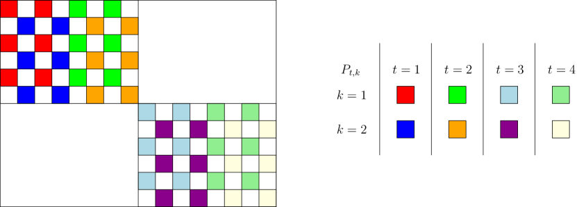
Figure 6: The partition $\mathcal{P}_{\mathtt{col}}({\boldsymbol{\pi}},r)$ with ${\boldsymbol{\pi}}=(2,3,4,2)$ and $r=2$. Each set $P_{t,k},(t,k)\in\llbracket 4\rrbracket\times\llbracket 2\rrbracket$ gathers the indices of the columns of $\mathbf{S}_{\boldsymbol{\pi}}$ of a given color. See also Figure 1. Same color indicates columns of the same sets $P_{t,k}$ (cf. Definition C.10).

Proof C.11 (Proof of Lemma C.7).

It is easy to check that $\mathcal{P}^{\prime}:=\mathcal{P}_{\mathtt{col}}({\boldsymbol{\pi}},r)$ partitions the index set $\llbracket q\rrbracket$, with $q=acd$, into $|\mathcal{P}^{\prime}|=acd/r$ components $P=P_{t,k}\in\mathcal{P}^{\prime}$ of equal cardinality $|P|=r$. Since, by Lemma 4.9, the partition $\mathcal{P}:=\mathcal{P}(\mathbf{S}_{{\boldsymbol{\pi}}},\mathbf{S}_{{\boldsymbol{\pi}}^{\prime}})$ of $\llbracket q\rrbracket$ has the same property, it is sufficient to prove that, for any $P\in\mathcal{P}$, there exists $(t,k)\in\llbracket ac/r\rrbracket\times\llbracket d\rrbracket$ such that $P=P_{t,k}$ (such a pair $(t,k)$ is necessarily unique since we consider partitions).

Given an arbitrary $P\in\mathcal{P}(\mathbf{S}_{{\boldsymbol{\pi}}},\mathbf{S}_{{{\boldsymbol{\pi}}}^{\prime}})$, we prove first that there exists a unique $t\in\llbracket ac/r\rrbracket$ such that $P\subseteq P_{t}:=\bigcup_{k\in\llbracket d\rrbracket}P_{t,k}$. Notice (see also Figure 6) that each $P_{t}$ is an interval of length $dr$ and since (by chainability of $({\boldsymbol{\pi}},{{\boldsymbol{\pi}}}^{\prime})$) we have $acd={a}^{\prime}{b}^{\prime}{d}^{\prime}$, $ac/r={a}^{\prime}$, and $dr={b}^{\prime}{d}^{\prime}$,

(42) $$P_{t}=\llbracket(t-1)dr+1,tdr\rrbracket=\llbracket(t-1)b^{\prime}d^{\prime}+1,tb^{\prime}d^{\prime}\rrbracket.$$

Further observe that $\{P_{t}\}_{t\in\llbracket ac/r\rrbracket}$ partitions $\llbracket q\rrbracket=\llbracket{a}^{\prime}{b}^{\prime}{d}^{\prime}\rrbracket$ into ${a}^{\prime}$ consecutive intervals of length ${b}^{\prime}{d}^{\prime}$. In other words, $P_{t}$ indexes the rows of the $t$-th block of $\mathbf{S}_{{\boldsymbol{\pi}}^{\prime}}$, cf. Figure 1. As a result, there exists at least one index $t$ such that $P_{t}\cap P\neq\emptyset$. We next prove the uniqueness of such a $t$, which implies $P\subseteq P_{t}$ as we consider a partition of $\llbracket q\rrbracket$. Consider two indices $t,t^{\prime}$ such that $P_{t}\cap P\neq\emptyset$ and $P_{t^{\prime}}\cap P\neq\emptyset$, and $i\in P_{t}\cap P$, $i^{\prime}\in P_{t^{\prime}}\cap P$. By Definition 3.3, since $i,i^{\prime}\in P$ and $P\in\mathcal{P}(\mathbf{S}_{{\boldsymbol{\pi}}},\mathbf{S}_{{{\boldsymbol{\pi}}}^{\prime}})$, we have $\mathbf{S}_{{{\boldsymbol{\pi}}}^{\prime}}[i,:]=\mathbf{S}_{{{\boldsymbol{\pi}}}^{\prime}}[i^{\prime},:]$. Since $\mathbf{S}_{{\boldsymbol{\pi}}^{\prime}}=\mathbf{I}_{a^{\prime}}\otimes\mathbf{1}_{b^{\prime}\times c^{\prime}}\otimes\mathbf{I}_{d^{\prime}}$ is block-diagonal with $a^{\prime}$ blocks of size $b^{\prime}d^{\prime}\times c^{\prime}d^{\prime}$, the row $\mathbf{S}_{{{\boldsymbol{\pi}}}^{\prime}}[i,:]$ is supported in a subset of the interval $\llbracket(\ell-1)c^{\prime}d^{\prime}+1,\ell c^{\prime}d^{\prime}\rrbracket$ with $\ell\in\llbracket a^{\prime}\rrbracket$ the unique integer such that $i\in\llbracket(\ell-1)b^{\prime}d^{\prime}+1,\ell b^{\prime}d^{\prime}\rrbracket=P_{\ell}$. Since $i\in P_{t}$ we have $\ell=t$. The same holds for $\mathbf{S}_{{{\boldsymbol{\pi}}}^{\prime}}[i^{\prime},:]$ with $\ell^{\prime}=t^{\prime}$. Since both rows are identical, we deduce that $\ell=\ell^{\prime}$, hence $t=t^{\prime}$.

Considering now the unique $t\in\llbracket ac/r\rrbracket$ such that $P\subseteq{P_{t}}$, since $\{P_{t,k}\}_{k\in\llbracket d\rrbracket}$ partitions $P_{t}$, there must exist $k\in\llbracket d\rrbracket$ such that $P_{t,k}\cap P\neq\emptyset$. Again, we now prove the uniqueness of such a $k$, which implies that $P\subseteq P_{t,k}$, and since $|P|=q=|P_{t,k}|$, we will obtain $P=P_{t,k}$ as claimed. Consider two indices $k,k^{\prime}\in\llbracket d\rrbracket$ such that $P_{t,k}\cap P\neq\emptyset$ and $P_{t,k^{\prime}}\cap P\neq\emptyset$, and $i\in P\cap P_{t,k}$ and $i^{\prime}\in P\cap P_{t,k^{\prime}}$. By construction (see Definition C.10), we have ${i\equiv k\mod d}$ and ${i\equiv k^{\prime}\mod d}$. To continue we observe that $\{P_{t,k}\}_{k\in\llbracket d\rrbracket}$ partitions the interval $P_{t}$ into $d$ (disjoint) subsets of integers of cardinality $r$ and the elements in such subsets are equally spaced by a distance $d$. Moreover, as above, since $i,i^{\prime}\in P$ and $P\in\mathcal{P}(\mathbf{S}_{\boldsymbol{\pi}},\mathbf{S}_{{\boldsymbol{\pi}}^{\prime}})$, we have $\mathbf{S}_{{\boldsymbol{\pi}}}[:,i]=\mathbf{S}_{{\boldsymbol{\pi}}}[:,i^{\prime}]$. By the structure $\mathbf{S}_{{\boldsymbol{\pi}}}=\mathbf{I}_{a}\otimes\mathbf{1}_{b\times c}\otimes\mathbf{I}_{d}$, for each $k$ the columns of $\mathbf{S}_{\boldsymbol{\pi}}$ such that $\mathtt{supp}(\mathbf{S}[{:,{i}}])\subseteq P_{t,k}$ share in fact the same support, which is disjoint from the other column supports (see illustration of Fig. 6).

Finally, by Definition 4.6 and chainability of $({\boldsymbol{\pi}},{\boldsymbol{\pi}}^{\prime})$, we have $r=r({\boldsymbol{\pi}},{\boldsymbol{\pi}}^{\prime})=ac/a^{\prime}$, so that $|\mathcal{P}|=|\mathcal{P}^{\prime}|=acd/r=a^{\prime}d$ as claimed.

We conclude the section with a lemma that relates $\mathcal{P}_{\mathtt{col}}(\cdot,r)$ for various patterns.

Lemma C.12.

Consider a chainable architecture ${\boldsymbol{\beta}}=({\boldsymbol{\pi}}_{\ell})_{\ell=1}^{L}$ and a natural number $r\mid c_{L}$ where ${\boldsymbol{\pi}}_{L}=(a_{L},b_{L},c_{L},d_{L})$. Then $r\mid c$ where ${\boldsymbol{\pi}}_{1}*\ldots*{\boldsymbol{\pi}}_{L}=(a,b,c,d)$, and $\mathcal{P}_{\mathtt{col}}({\boldsymbol{\pi}}_{1}*\ldots*{\boldsymbol{\pi}}_{L},r)=\mathcal{P}_{\mathtt{col}}({\boldsymbol{\pi}}_{L},r)$.

Proof C.13.

We prove the result for $L=2$. The general case follows by induction. Consider ${\boldsymbol{\pi}}_{i}=(a_{i},b_{i},c_{i},d_{i})$, with $i\in\llbracket 2\rrbracket$, and an integer $r\mid c_{2}$. By definition of the $*$ operator in Equation 9 we have

$$(a,b,c,d):={\boldsymbol{\pi}}_{1}*{\boldsymbol{\pi}}_{2}=\left(a_{1},\frac{b_{1}d_{1}}{d_{2}},\frac{a_{2}c_{2}}{a_{1}},d_{2}\right)$$

Since $({\boldsymbol{\pi}}_{1},{\boldsymbol{\pi}}_{2})$ are chainable, we have $a_{1}\mid a_{2}$. Since $r\mid c_{2}$, we have $r\mid(a_{2}/a_{1})c_{2}$, i.e., $r\mid c$ as claimed. A direct calculation then shows that $\mathcal{P}_{\mathtt{col}}({\boldsymbol{\pi}}_{2},r)=\mathcal{P}_{\mathtt{col}}({\boldsymbol{\pi}}_{1}*{\boldsymbol{\pi}}_{2},r)$, since for each $t\in\llbracket ac/r\rrbracket=\llbracket a_{2}c_{2}/r\rrbracket$, $k\in\llbracket d\rrbracket=\llbracket d_{2}\rrbracket$, (41) yields the very same set $P_{t,k}$ (as $dr=d_{2}r$ and $d=d_{2}$).

C.2.1 Proof of Lemma 6.3

This is a direct corollary of Lemma C.14 below.

With the notations of Lemma 6.3, the constant $r$ involved in Lemma C.14 applied to ${\boldsymbol{\pi}}={\boldsymbol{\pi}}_{I_{i}}$ and ${\boldsymbol{\pi}}^{\prime}={\boldsymbol{\pi}}_{I_{i+1}}$ for $i=1,\ldots,j-1$ is indeed equal to $r({\boldsymbol{\pi}}_{t_{i}},{\boldsymbol{\pi}}_{t_{i}+1})$:

1. The intervals $I_{i}:=\llbracket q_{i},t_{i}\rrbracket$ in partition are a sorted partition of $\llbracket 1,L\rrbracket$. Therefore, $t_{i}+1=q_{i+1}$ for each $i$.

2. By  Lemma 4.16, $r({\boldsymbol{\pi}}_{I_{i}},{\boldsymbol{\pi}}_{I_{i+1}})=r({\boldsymbol{\pi}}_{t_{i}},{\boldsymbol{\pi}}_{q_{i+1}})=r({\boldsymbol{\pi}}_{t_{i}},{\boldsymbol{\pi}}_{t_{i}+1})$.

Lemma C.14.

Consider a non-redundant chainable pair $({\boldsymbol{\pi}},{\boldsymbol{\pi}}^{\prime})$, and $(\mathbf{X},\mathbf{Y})\in\Sigma^{{\boldsymbol{\pi}}}\times\Sigma^{{\boldsymbol{\pi}}^{\prime}}$. Denote $r:=r({\boldsymbol{\pi}},{\boldsymbol{\pi}}^{\prime})$. Algorithm 5 with input $u\in\{\texttt{column},\texttt{row}\}$ returns $(\tilde{\mathbf{X}},\tilde{\mathbf{Y}})\in\Sigma^{{\boldsymbol{\pi}}}\times\Sigma^{{\boldsymbol{\pi}}^{\prime}}$ such that $\tilde{\mathbf{X}}\tilde{\mathbf{Y}}=\mathbf{X}\mathbf{Y}$ and:

• if $u=\texttt{column}$ then $\tilde{\mathbf{X}}$ is left-$r$-unitary;

• otherwise if $u=\texttt{row}$ then $\tilde{\mathbf{Y}}$ is right-$r$-unitary.

Proof C.15.

We only prove the first point, as the second point can be addressed similarly. Denoting $\mathcal{P}=\mathcal{P}(\mathbf{S}_{{\boldsymbol{\pi}}},\mathbf{S}_{{\boldsymbol{\pi}}^{\prime}})$, by Lemma 4.9, for any $(\tilde{\mathbf{X}},\tilde{\mathbf{Y}})\in\Sigma^{{\boldsymbol{\pi}}}\times\Sigma^{{\boldsymbol{\pi}}^{\prime}}$, $\mathtt{supp}(\mathbf{X}\mathbf{Y})$ and $\mathtt{supp}(\tilde{\mathbf{X}}\tilde{\mathbf{Y}})$ are both included in $\bigcup_{P\in\mathcal{P}}R_{P}\times C_{P}$ where $\{R_{P}\times C_{P}\}_{P\in\mathcal{P}}$ are pairwise disjoint. As a result, we have:

$$\begin{split}\mathbf{X}\mathbf{Y}=\tilde{\mathbf{X}}\tilde{\mathbf{Y}}&\iff\forall P\in\mathcal{P},\quad(\mathbf{X}\mathbf{Y})[R_{P},C_{P}]=(\tilde{\mathbf{X}}\tilde{\mathbf{Y}})[R_{P},C_{P}]\\ &\iff\forall P\in\mathcal{P},\quad(\mathbf{X}\mathbf{Y})[R_{P},C_{P}]=\tilde{\mathbf{X}}[R_{P},P]\tilde{\mathbf{Y}}[P,C_{P}],\end{split}$$

where the second equivalence comes by Lemma A.1 and by chainability of $({\boldsymbol{\pi}}_{1},{\boldsymbol{\pi}}_{2})$. Moreover, by Theorem C.8, $\tilde{\mathbf{X}}\in\Sigma^{{\boldsymbol{\pi}}}$ is left-$r$-unitary if, and only if, $\tilde{\mathbf{X}}[R_{P},P]$ has orthonormal columns for each $P\in\mathcal{P}_{\mathtt{col}}({\boldsymbol{\pi}},r)=\mathcal{P}(\mathbf{S}_{{\boldsymbol{\pi}}},\mathbf{S}_{{\boldsymbol{\pi}}^{\prime}})=\mathcal{P}$.

The output $(\tilde{\mathbf{X}},\tilde{\mathbf{Y}})$ of Algorithm 5 is built via the QR-decomposition of ${\mathbf{X}}[R_{P},P]=\mathbf{Q}\mathbf{R}$, and setting $\tilde{\mathbf{X}}[R_{P},P]=\mathbf{Q}$, $\tilde{\mathbf{Y}}[P,C_{P}]=\mathbf{R}\mathbf{Y}[P,C_{P}]$, which is possible because $({\boldsymbol{\pi}},{\boldsymbol{\pi}}^{\prime})$ is assumed to be non-redundant. Indeed, to enable $\mathbf{Q}\in\mathbb{R}^{|R_{P}|\times|P|}$ to have orthonormal columns, we must have $|R_{P}|\geq|P|$, or equivalently, $b\geq q$ (assuming that ${\boldsymbol{\pi}}=(a,b,c,d)$, see Lemma 4.9). This is the non-redundancy criterion (cf. Definition 4.17). Thus, $\tilde{\mathbf{X}}[R_{P},P]$ has orthonormal columns and $\tilde{\mathbf{X}}[R_{P},P]\tilde{\mathbf{Y}}[P,C_{P}]=\mathbf{Q}\mathbf{R}\mathbf{Y}[P,C_{P}]=\mathbf{X}[R_{P},P]\mathbf{Y}[P,C_{P}]=(\mathbf{X}\mathbf{Y})[R_{P},C_{P}]$.

C.2.2 Further useful technical properties of $r$-unitary factors

Lemma C.16.

Let $\mathbf{X}$ be a left-$r$-unitary ${\boldsymbol{\pi}}$-factor with ${\boldsymbol{\pi}}={(a,b,c,d)}$. For any $t\in\llbracket ac/r\rrbracket$, the submatrix $\mathbf{X}[:,P_{t}]$ with $P_{t}$ as in (42) has orthonormal columns.

Proof C.17.

From the proof of Lemma C.7 the sets $(P_{t,k})_{k\in\llbracket d\rrbracket}$ from Definition C.10 partition $P_{t}$ into $d$ subsets of integers of cardinality $r$ and the elements of each subsets are equally spaced by a distance $d$. We first show that the columns of $\mathbf{X}[{:,{P_{t}}}]$ coming from distinct blocks $P:=P_{t,k}$, $P^{\prime}:=P_{t,k^{\prime}}$ (where $1\leq k\neq k^{\prime}\leq d$) are mutually orthogonal, as they have disjoint supports. Due to the structure of $\mathbf{S}_{\boldsymbol{\pi}}=\mathbf{I}_{a}\otimes\mathbf{1}_{b\times c}\otimes\mathbf{I}_{d}$, if two columns share the same support, the difference of their indices is divisible by $d$. Otherwise, their supports are disjoint. Thus, $P$ and $P^{\prime}$ have disjoint column supports.

To conclude we show that each submatrix $\mathbf{X}[{:,{P_{t,k}}}]$ has orthonormal columns. Indeed, by Definition C.10, we have $P:=P_{t,k}\in\mathcal{P}_{\mathtt{col}}({\boldsymbol{\pi}},r)$, hence by Theorem C.8 the block $\mathbf{X}[R_{P},P]$ has orthonormal columns. Since $R_{P}$ is the support of the columns of $\mathbf{S}_{{\boldsymbol{\pi}}}[{:,{P}}]$, and as $\mathtt{supp}(\mathbf{X})\subseteq\mathtt{supp}(\mathbf{S}_{\boldsymbol{\pi}})$, the submatrix $\mathbf{X}[{:,{P}}]$ is zero outside of the block $\mathbf{X}[R_{P},P]$ hence it also has orthonormal columns.

Remark C.18.

Although the columns of $\mathbf{X}[{:,{P_{t}}}]$ are orthonormal and the sets $P_{t}$ are pairwise disjoint, it does not imply that $\mathbf{X}$ has orthonormal columns. For example, consider the sets $P_{1}$ (indices of columns in red and blue) and $P_{2}$ (columns in green and orange) illustrated in Fig. 6. Even though these two sets are disjoint the supports of their columns are not. Thus, the matrix can be left-$2$-unitary without having orthonormal columns. This example also explains our earlier Remark 6.2.

Corollary C.19.

Consider a chainable pair of patterns $({\boldsymbol{\pi}},{\boldsymbol{\pi}}^{\prime})$. If $\mathbf{X}\in\Sigma^{{\boldsymbol{\pi}}}$ is left-$r({\boldsymbol{\pi}},{\boldsymbol{\pi}}^{\prime})$-unitary, then for any column index $i$ of $\mathbf{S}_{{\boldsymbol{\pi}}^{\prime}}$ the submatrix $\mathbf{X}[{:,{T_{i}}}]$, where $T_{i}=\mathtt{supp}(\mathbf{S}_{{\boldsymbol{\pi}}^{\prime}}[{:,{i}}])$, has orthonormal columns.

Proof C.20.

Denote ${\boldsymbol{\pi}}=(a,b,c,d)$, ${\boldsymbol{\pi}}^{\prime}=(a^{\prime},b^{\prime},c^{\prime},d^{\prime})$, $r=r({\boldsymbol{\pi}},{\boldsymbol{\pi}}^{\prime})$. Since $\mathbf{S}_{{\boldsymbol{\pi}}^{\prime}}=\mathbf{I}_{a^{\prime}}\otimes\mathbf{1}_{b^{\prime}\times c^{\prime}}\otimes\mathbf{I}_{d^{\prime}}$ is block-diagonal with $a^{\prime}$ blocks of size $b^{\prime}d^{\prime}\times c^{\prime}d^{\prime}$, the set $T_{i}$ is a subset of the interval $P_{t}=\llbracket(t-1)b^{\prime}d^{\prime}+1,tb^{\prime}d^{\prime}\rrbracket$ with $t\in\llbracket a^{\prime}\rrbracket$ the unique integer such that $i\in\llbracket(t-1)c^{\prime}d^{\prime},tc^{\prime}d^{\prime}\rrbracket$. By chainability of $({\boldsymbol{\pi}},{\boldsymbol{\pi}}^{\prime})$ we have $b^{\prime}d^{\prime}=dr$. By Lemma C.16, $\mathbf{X}[:,P_{t}]$ has orthonormal columns, and therefore so does $\mathbf{X}[:,T_{i}]$.

The following corollary will be handy to prove (53), in the proof of Lemma E.1.

Corollary C.21.

Consider a chainable architecture of ${\boldsymbol{\beta}}=({\boldsymbol{\pi}}_{1},\ldots,{\boldsymbol{\pi}}_{L})$. Denote

$${\boldsymbol{\pi}}_{1}^{\prime}:={\boldsymbol{\pi}}_{1}*\ldots*{\boldsymbol{\pi}}_{q-1},\quad{\boldsymbol{\pi}}_{2}^{\prime}:={\boldsymbol{\pi}}_{q}*\ldots*{\boldsymbol{\pi}}_{t},\quad{\boldsymbol{\pi}}_{3}^{\prime}:={\boldsymbol{\pi}}_{t+1}*\ldots*{\boldsymbol{\pi}}_{L}.$$

If $\mathbf{X}\in\Sigma^{{\boldsymbol{\pi}}^{\prime}_{1}}$ and $\mathbf{Z}\in\Sigma^{{\boldsymbol{\pi}}^{\prime}_{3}}$ are respectively left-$r({\boldsymbol{\pi}}_{1}^{\prime},{\boldsymbol{\pi}}_{2}^{\prime})$-unitary and right-$r({\boldsymbol{\pi}}_{2}^{\prime},{\boldsymbol{\pi}}_{3}^{\prime})$-unitary, then $\mathbf{X}[{:,{R}}]$ (resp. $\mathbf{Z}[{{C},:}]$) has orthonormal columns (resp. rows) for any column (resp. row) support $R$ (resp. $C$) of $\mathbf{S}_{{\boldsymbol{\pi}}_{2}^{\prime}}$, i.e., whenever $R=\mathtt{supp}(\mathbf{S}_{{\boldsymbol{\pi}}_{2}^{\prime}}[{:,{i}}])$ (resp. $C=\mathtt{supp}(\mathbf{S}_{{\boldsymbol{\pi}}_{2}^{\prime}}[{{i},:}])$) for some row (resp. column) index $i$.

Proof C.22.

We consider the case of columns of $\mathbf{X}[{:,{R}}]$. The other case can be dealt with similarly. The proof follows from Corollary C.19 because:

1. By Lemma 4.16, $({\boldsymbol{\pi}}_{1}^{\prime},{\boldsymbol{\pi}}_{2}^{\prime})$ is chainable with $r({\boldsymbol{\pi}}_{1}^{\prime},{\boldsymbol{\pi}}_{2}^{\prime})=r({\boldsymbol{\pi}}_{q-1},{\boldsymbol{\pi}}_{q})$;

2. $\mathbf{X}$ is a left-$r({\boldsymbol{\pi}}_{1}^{\prime},{\boldsymbol{\pi}}_{2}^{\prime})$-unitary ${\boldsymbol{\pi}}^{\prime}_{1}$-factor;

3. $R=\mathtt{supp}(\mathbf{S}_{{\boldsymbol{\pi}}_{2}^{\prime}}[:,i])$ for some column index $i$.

Appendix D Complexity of hierarchical algorithms - proof of Theorem 6.5

We analyze the complexity of each of the components involved in the proposed hierarchical algorithms.

D.1 Complexity of Algorithm 1

This algorithm essentially performs several low-rank approximations that are typically computed using truncated SVD.

Lemma D.1.

Consider $(\mathbf{L},\mathbf{R})$ satisfying the condition of Theorem 3.4. For any matrix $\mathbf{A}$, the complexity of the two-factor fixed support matrix factorization algorithm (Algorithm 1) with input $\mathbf{A},\mathbf{L},\mathbf{R}$ is

$$\mathcal{O}\left(\sum_{P\in\mathcal{P}(\mathbf{L},\mathbf{R})}|P||R_{P}||C_{P}|\right).$$

Proof D.2.

The algorithm performs the best rank-$|P|$ approximation of a submatrix of size $|R_{P}|\times|C_{P}|$ for each $P\in\mathcal{P}(\mathbf{L},\mathbf{R})$ and the complexity of the truncated SVD at order $k$ for an $m\times n$ matrix is $\mathcal{O}(kmn)$ [16].

We apply this complexity analysis to the case where $(\mathbf{L},\mathbf{R})$ are butterfly supports corresponding to a chainable pair of patterns.

Lemma D.3.

Consider chainable patterns ${\boldsymbol{\pi}}=(a,b,c,d)$, ${\boldsymbol{\pi}}^{\prime}=(a^{\prime},b^{\prime},c^{\prime},d^{\prime})$. Denoting $r:=r({\boldsymbol{\pi}},{\boldsymbol{\pi}}^{\prime})$, the complexity $C({\boldsymbol{\pi}},{\boldsymbol{\pi}}^{\prime})$ of the two-factor fixed support matrix factorization algorithm (Algorithm 1) with input $\mathbf{A},\mathbf{S}_{{\boldsymbol{\pi}}},\mathbf{S}_{{\boldsymbol{\pi}}^{\prime}}$ is

(43) $$C({\boldsymbol{\pi}},{\boldsymbol{\pi}}^{\prime})=\mathcal{O}(ra^{\prime}bc^{\prime}d).$$

Proof D.4.

By Lemma 4.9, for each $P\in\mathcal{P}:=\mathcal{P}(\mathbf{S}_{\boldsymbol{\pi}},\mathbf{S}_{{\boldsymbol{\pi}}^{\prime}})$ we have $|P|=r$, $|R_{P}|=b$ and $|C_{P}|=c^{\prime}$. By Lemma C.7 we have $|\mathcal{P}|=a^{\prime}d$. By Lemma D.1 it follows that $C({\boldsymbol{\pi}},{\boldsymbol{\pi}}^{\prime})=\mathcal{O}(a^{\prime}drbc^{\prime})$.

Remark D.5.

In practice, best low-rank approximations in Algorithm 1 via truncated SVDs can be computed in parallel. For arbitrary $\mathbf{L},\mathbf{R}$ as in Lemma D.1 this can decrease the complexity down to $\mathcal{O}(\max_{P\in\mathcal{P}(\mathbf{L},\mathbf{R})}|P||R_{P}||C_{P}|)$ when parallelizing accross $|\mathcal{P}(\mathbf{L},\mathbf{R})|$ processes. For butterfly factors as in Lemma D.3, this decreases the complexity down to $\mathcal{O}(rbc^{\prime})$.

D.2 Complexity of Algorithm 3

This algorithm is based on Algorithm 1. We prove the first point of Theorem 6.5 in the following lemma.

Lemma D.6.

Consider a non-redundant chainable architecture ${\boldsymbol{\beta}}$ and a matrix $\mathbf{A}$ of size $m\times n$. With notations of Theorem 6.5, the complexity of the hierarchical algorithm (Algorithm 3) with inputs ${\boldsymbol{\beta}}$, $\mathbf{A}$ and any factor-bracketing tree $\mathcal{T}$ is at most:

• $\mathcal{O}(\|\mathbf{r}({\boldsymbol{\beta}})\|_{1}M_{\boldsymbol{\beta}}N_{\boldsymbol{\beta}})$ in the general case;

• $\mathcal{O}(\|\mathbf{r}({\boldsymbol{\beta}})\|_{1}mn)$ if ${\boldsymbol{\beta}}$ is non-redundant.

Proof D.7.

Since Algorithm 3 performs $(L-1)$ factorizations of the form of Problem (17) using the two-factor fixed-support matrix factorization algorithm (Algorithm 1), its complexity is equal to the sum of the complexity of each of these $(L-1)$ factorizations.

Fix $1\leq q\leq s<t\leq L$. By Lemma 4.16, $r_{s}:=r({\boldsymbol{\pi}}_{q}*\ldots*{\boldsymbol{\pi}}_{s},{\boldsymbol{\pi}}_{s+1}*\ldots*{\boldsymbol{\pi}}_{t})=r({\boldsymbol{\pi}}_{s},{\boldsymbol{\pi}}_{s+1})$. By (11) we have

$${\boldsymbol{\pi}}_{q}*\ldots*{\boldsymbol{\pi}}_{s}=\left(a_{q},\frac{b_{q}d_{q}}{d_{s}},\frac{a_{s}c_{s}}{a_{q}},d_{s}\right),\ {\boldsymbol{\pi}}_{s+1}*\ldots*{\boldsymbol{\pi}}_{t}=\left(a_{s+1},\frac{b_{s+1}d_{s+1}}{d_{t}},\frac{a_{t}c_{t}}{a_{s+1}},d_{t}\right),$$

hence, Lemma D.3 yields $C({\boldsymbol{\pi}}_{q}*\ldots*{\boldsymbol{\pi}}_{s},{\boldsymbol{\pi}}_{s+1}*\ldots*{\boldsymbol{\pi}}_{t})=\mathcal{O}(r_{s}a_{t}c_{t}b_{q}d_{q})$, which is upper bounded by $\mathcal{O}(r_{s}M_{\boldsymbol{\beta}}N_{\boldsymbol{\beta}})$, by definition of $M_{\boldsymbol{\beta}}:=\max_{\ell}a_{\ell}c_{\ell},N_{\boldsymbol{\beta}}:=\max_{\ell}b_{\ell}d_{\ell}$. Therefore, the overall complexity of Algorithm 3 is upper bounded by:

(44) $$\sum_{s=1}^{L-1}\mathcal{O}(r_{s}M_{\boldsymbol{\beta}}N_{\boldsymbol{\beta}})=\mathcal{O}(\|\mathbf{r}({\boldsymbol{\beta}})\|_{1}M_{\boldsymbol{\beta}}N_{\boldsymbol{\beta}}).$$

When ${\boldsymbol{\beta}}$ is non-redundant, by Definition 4.17 we have $a_{\ell}c_{\ell}<a_{\ell+1}c_{\ell+1}$ and $b_{\ell}d_{\ell}>b_{\ell+1}d_{\ell+1}$ for all $\ell\in\llbracket L-1\rrbracket$. Since $m=a_{1}b_{1}d_{1}$ and $n=a_{L}c_{L}d_{L}$ (cf. Lemma 4.13 and Definition 4.1) we obtain $M_{\boldsymbol{\beta}}=\max_{\ell}a_{\ell}c_{\ell}<a_{L}c_{L}=n/d_{L}\leq n$ and $N_{\boldsymbol{\beta}}=\max_{\ell}b_{\ell}d_{\ell}<b_{1}d_{1}=m/a_{1}\leq m$.

D.3 Complexity of Algorithm 5

We now analyze the complexity of the construction of orthonormal butterfly factors in Algorithm 5.

Lemma D.8.

The complexity of column/row-pseudo-orthonormalization (Algorithm 5) with input $({\boldsymbol{\pi}}_{1},{\boldsymbol{\pi}}_{2},\mathbf{X},\mathbf{Y},u)$ for any $u\in\{\texttt{column},\texttt{row}\}$ and any non-redundant chainable pair $({\boldsymbol{\pi}}_{1},{\boldsymbol{\pi}}_{2})$ is

$$\mathcal{O}(r({\boldsymbol{\pi}}_{1},{\boldsymbol{\pi}}_{2})(\|{\boldsymbol{\pi}}_{1}\|_{0}+\|{\boldsymbol{\pi}}_{2}\|_{0})),$$

with the notation $\|{\boldsymbol{\pi}}\|_{0}$ from Lemma 4.3.

Proof D.9.

We only consider the case $u=\texttt{column}$, since the other case can be dealt with similarly. Denote $r=r({\boldsymbol{\pi}}_{1},{\boldsymbol{\pi}}_{2})$ and ${\boldsymbol{\pi}}_{\ell}=(a_{\ell},b_{\ell},c_{\ell},d_{\ell})$ for $\ell\in\llbracket 2\rrbracket$. By Lemma 4.9 for each $P\in\mathcal{P}(\mathbf{S}_{\boldsymbol{\pi}},\mathbf{S}_{{\boldsymbol{\pi}}^{\prime}})$ we have $|P|=r$, $|R_{P}|=b_{1}$, $|C_{P}|=c_{2}$, and we have $r\leq\min(b_{1},c_{2})$ (cf. Definition 4.6). Thus, at each iteration of Algorithm 5:

• the complexity of line 4 is $\mathcal{O}(|R_{P}||P|^{2})=\mathcal{O}(b_{1}r^{2})$, since the complexity of QR-decomposition of an $m\times n$ matrix is $\mathcal{O}(\min(m,n)mn)$ [12, Section 5.2];

• the complexity of line 5 is $\mathcal{O}(|R_{P}||P|)=\mathcal{O}(b_{1}r)$;

• the complexity of line 6 is $\mathcal{O}(|P|^{2}|C_{P}|)=\mathcal{O}(c_{2}r^{2})$.

Overall, the complexity of an iteration is $\mathcal{O}(r^{2}(b_{1}+c_{2}))$. There are $a_{1}c_{1}d_{1}/r=a_{2}b_{2}d_{2}/r$ equivalence classes (by Lemma C.7 and chainability, that implies $a_{1}c_{1}d_{1}=a_{2}b_{2}d_{2}$, see Definition 4.6), and by Lemma 4.3 $a_{\ell}b_{\ell}c_{\ell}d_{\ell}=\|{\boldsymbol{\pi}}_{\ell}\|_{0}$, hence the overall complexity is

$$\begin{split}\mathcal{O}\left(\frac{a_{1}c_{1}d_{1}}{r}r^{2}b_{1}+\frac{a_{2}b_{2}d_{2}}{r}r^{2}c_{2}\right)&=\mathcal{O}(r(a_{1}b_{1}c_{1}d_{1}+a_{2}b_{2}c_{2}d_{2}))\\ &=\mathcal{O}(r({\boldsymbol{\pi}}_{1},{\boldsymbol{\pi}}_{2})(\|{\boldsymbol{\pi}}_{1}\|_{0}+\|{\boldsymbol{\pi}}_{2}\|_{0})).\end{split}$$

D.4 Complexity of Algorithm 4

We can now prove the second point of Theorem 6.5, where we assume that ${\boldsymbol{\beta}}$ is not redundant so that $M_{\boldsymbol{\beta}}\leq m$ and $N_{\boldsymbol{\beta}}\leq n$. By Lemma D.8 the complexity for each call to Algorithm 5 in lines 12 and 15 of the new butterfly algorithm (Algorithm 4) is given by $\mathcal{O}(r({\boldsymbol{\pi}}_{I_{k-1}},{\boldsymbol{\pi}}_{I_{k}})(\|{\boldsymbol{\pi}}_{I_{k-1}}\|_{0}+\|{\boldsymbol{\pi}}_{I_{k}}\|_{0}))$ where ${\boldsymbol{\pi}}_{I}={\boldsymbol{\pi}}_{q}*\ldots{\boldsymbol{\pi}}_{s}$ if $I:=\llbracket q,s\rrbracket$. By Lemma 4.16, $r({\boldsymbol{\pi}}_{I_{k-1}},{\boldsymbol{\pi}}_{I_{k}})=r({\boldsymbol{\pi}}_{s},{\boldsymbol{\pi}}_{s+1})$ for some $1\leq s\leq L-1$, thus is bounded by $\|r({\boldsymbol{\beta}})\|_{\infty}$ (cf. Definition 4.11). Moreover, ${\boldsymbol{\pi}}_{I_{k}}$ (resp. ${\boldsymbol{\pi}}_{I_{k-1}}$) has the form $(a_{q},\frac{b_{q}d_{q}}{d_{s}},\frac{a_{s}c_{s}}{a_{q}},d_{s})$ for some $1\leq q\leq s\leq L$ (cf. Lemma 4.13). Thus, $\|{\boldsymbol{\pi}}_{I_{k}}\|_{0}$ (resp. $\|{\boldsymbol{\pi}}_{I_{k-1}}\|_{0}$) is bounded (recall the notation $\|{\boldsymbol{\pi}}\|_{0}$ from Lemma 4.3) by $\max_{q,s}b_{q}d_{q}a_{s}c_{s}\leq M_{\boldsymbol{\beta}}N_{\boldsymbol{\beta}}\leq mn$. In conclusion, the complexity of each call to Algorithm 5 is at most $\mathcal{O}(mn\|\mathbf{r}({\boldsymbol{\beta}})\|_{\infty})$. At the $J$-th iteration for some $J\in\llbracket L-1\rrbracket$, there are at most $(J-1)$ calls to Algorithm 5, so the total complexity for the orthonormalization operations accross all the $|{\boldsymbol{\beta}}|-1$ iterations is at most $\mathcal{O}(|{\boldsymbol{\beta}}|^{2}mn\|\mathbf{r}({\boldsymbol{\beta}})\|_{\infty})$. Therefore, the complexity of Algorithm 4 is given by

$$\mathcal{O}\left((|{\boldsymbol{\beta}}|^{2}\|\mathbf{r}({\boldsymbol{\beta}})\|_{\infty}+\|\mathbf{r}({\boldsymbol{\beta}})\|_{1})mn\right).$$

Appendix E Proof of the results of Section 7

E.1 Proof of Lemma 7.13

First, we prove that $\mathbf{B}^{\prime}\in\mathcal{B}^{{\boldsymbol{\beta}}_{s}}$. By definition

$$\mathbf{B}^{\prime}=\underbrace{\left(\mathbf{X}_{P_{1}}\ldots\mathbf{X}_{P_{j-1}}\mathbf{X}_{\llbracket q,s\rrbracket}\right)}_{\mathbf{B}_{(\text{left})}^{\prime}}\underbrace{\left(\mathbf{X}_{\llbracket s+1,t\rrbracket}\mathbf{X}_{P_{j+1}}\ldots\mathbf{X}_{P_{J}}\right)}_{\mathbf{B}_{(\text{right})}^{\prime}}$$

and since by assumption $\mathbf{X}_{P_{i}}\in\Sigma^{{\boldsymbol{\pi}}_{q_{i}}*\ldots*{\boldsymbol{\pi}}_{t_{i}}}$ for every $i$, and ${\boldsymbol{\beta}}$ is chainable, a recursive application of Proposition 4.8 yields that $\mathbf{B}^{\prime}_{(\text{left})}\in\Sigma^{{\boldsymbol{\pi}}_{1}*\ldots*{\boldsymbol{\pi}}_{s}}$, $\mathbf{B}^{\prime}_{(\text{right})}\in\Sigma^{{\boldsymbol{\pi}}_{s+1}*\ldots*{\boldsymbol{\pi}}_{L}}$. Hence, $\mathbf{B}^{\prime}\in\mathcal{B}^{{\boldsymbol{\beta}}_{s}}$.

We now prove Equation 29. By Lemma 4.16 and chainability of ${\boldsymbol{\beta}}=({\boldsymbol{\pi}}_{\ell})_{\ell=1}^{L}$, the patterns ${\boldsymbol{\pi}}^{\prime}_{1}:={\boldsymbol{\pi}}_{1}*\ldots*{\boldsymbol{\pi}}_{q-1}$, ${\boldsymbol{\pi}}^{\prime}_{2}:={\boldsymbol{\pi}}_{q}*\ldots*{\boldsymbol{\pi}}_{t}$ and ${\boldsymbol{\pi}}^{\prime}_{3}:={\boldsymbol{\pi}}_{t+1}*\ldots*{\boldsymbol{\pi}}_{L}$ are well-defined, and the two-factor architectures ${\boldsymbol{\beta}}_{\mathtt{left}}:=({\boldsymbol{\pi}}^{\prime}_{1},{\boldsymbol{\pi}}^{\prime}_{2})$ and ${\boldsymbol{\beta}}_{\mathtt{right}}:=({\boldsymbol{\pi}}^{\prime}_{2},{\boldsymbol{\pi}}^{\prime}_{3})$ are both chainable with

$$r({\boldsymbol{\pi}}^{\prime}_{1},{\boldsymbol{\pi}}^{\prime}_{2})=r({\boldsymbol{\pi}}_{q-1},{\boldsymbol{\pi}}_{q})\ \text{and}\ r({\boldsymbol{\pi}}^{\prime}_{2},{\boldsymbol{\pi}}^{\prime}_{3})=r({\boldsymbol{\pi}}_{t},{\boldsymbol{\pi}}_{t+1}).$$

Moreover, by assumption, for each $i\in\llbracket j-1\rrbracket$ the factor $\mathbf{X}_{P_{i}}$ is left-$r({\boldsymbol{\pi}}_{t_{i}},{\boldsymbol{\pi}}_{t_{i}+1})$-unitary hence, using the notations $\mathbf{X}_{\mathrm{left}}^{(J)}$, $\mathbf{X}_{\mathrm{right}}^{(J)}$ of (27), multiple applications of Lemma C.3 yield that $\mathbf{X}_{\mathrm{left}}^{(J)}\in\Sigma^{{\boldsymbol{\pi}}^{\prime}_{1}}$ is left-$r({\boldsymbol{\pi}}_{r-1},{\boldsymbol{\pi}}_{r})$-unitary if $r\geq 2$ (if $r=1$ then by convention $\mathbf{X}_{\mathrm{left}}^{(J)}$ is the identity). Similarly, $\mathbf{X}_{\mathrm{right}}^{(J)}\in\Sigma^{{\boldsymbol{\pi}}^{\prime}_{3}}$ is right-$r({\boldsymbol{\pi}}_{t},{\boldsymbol{\pi}}_{t+1})$-unitary when $t\leq L-1$ (and the identity when $t=L$). Finally, by Proposition 4.8, both ${\mathbf{X}}_{\llbracket q,t\rrbracket}$ and ${\mathbf{X}}_{\llbracket q,s\rrbracket}{\mathbf{X}}_{\llbracket s+1,t\rrbracket}$ (and therefore their difference) belong to $\Sigma^{({\boldsymbol{\pi}}_{q}*\ldots*{\boldsymbol{\pi}}_{t})}=\Sigma^{{\boldsymbol{\pi}}^{\prime}_{2}}$, and denoting $\tilde{{\boldsymbol{\pi}}}_{1}:={\boldsymbol{\pi}}_{q}*\ldots*{\boldsymbol{\pi}}_{s-1}$ and $\tilde{{\boldsymbol{\pi}}}_{2}={\boldsymbol{\pi}}_{s+1}*\ldots*{\boldsymbol{\pi}}_{t}$, since ${\mathbf{X}}_{\llbracket q,s\rrbracket}$ and ${\mathbf{X}}_{\llbracket s+1,t\rrbracket}$ solve (17) we obtain

$$\|{\mathbf{B}}^{\prime}-{\mathbf{B}}\|_{F} =\|\mathbf{X}_{\mathrm{left}}^{(J)}({{\mathbf{X}}_{\llbracket q,t\rrbracket}}-{\mathbf{X}}_{\llbracket q,s\rrbracket}{\mathbf{X}}_{\llbracket s+1,t\rrbracket})\mathbf{X}_{\mathrm{right}}^{(J)}\|_{F}\hfill\quad\text{by definitions of }\mathbf{B},\mathbf{B}^{\prime}$$

$$=\|{{\mathbf{X}}_{\llbracket q,t\rrbracket}}-{\mathbf{X}}_{\llbracket q,s\rrbracket}{\mathbf{X}}_{\llbracket s+1,t\rrbracket}\|_{F}\hfill\quad\text{by \lx@cref{creftypecap~refnum}{lem:qunitarypreservesfrob}}$$

$$=\inf_{\mathbf{Y}_{i}\in\Sigma^{\tilde{{\boldsymbol{\pi}}}_{i}},i=1,2}\|{{\mathbf{X}}_{\llbracket q,t\rrbracket}}-\mathbf{Y}_{1}\mathbf{Y}_{2}\|_{F}\hfill\quad\text{by }\eqref{eq:fsmf-DB}$$

$$=E^{{{\boldsymbol{\beta}}}_{s}}(\mathbf{X}_{\mathrm{left}}^{(J)}\mathbf{X}_{\llbracket q,t\rrbracket}\mathbf{X}_{\mathrm{right}}^{(J)})\quad\text{by \lx@cref{creftypecap~refnum}{lem:originalkeylemma-new} below}$$

$$=E^{{{\boldsymbol{\beta}}}_{s}}({\mathbf{B}})\hfill\quad\text{by definition of }\mathbf{B}.$$

The penultimate line used the following result, which we prove next.

Lemma E.1.

Consider a non-redundant chainable architecture ${\boldsymbol{\beta}}:=({\boldsymbol{\pi}}_{\ell})_{\ell=1}^{L}$, integers $(q,s,t)$ such that $1\leq q\leq s<t\leq L$, and denote

$${\boldsymbol{\pi}}^{\prime}_{1}:={\boldsymbol{\pi}}_{1}*\ldots*{\boldsymbol{\pi}}_{q-1},\quad{\boldsymbol{\pi}}^{\prime}_{2}:={\boldsymbol{\pi}}_{q}*\ldots*{\boldsymbol{\pi}}_{t},\quad{\boldsymbol{\pi}}^{\prime}_{3}:={\boldsymbol{\pi}}_{t+1}*\ldots*{\boldsymbol{\pi}}_{L},$$

$$\tilde{{\boldsymbol{\pi}}}_{1}:={\boldsymbol{\pi}}_{q}*\ldots{\boldsymbol{\pi}}_{s},\quad\tilde{{\boldsymbol{\pi}}}_{2}:={\boldsymbol{\pi}}_{s+1}*\ldots*{\boldsymbol{\pi}}_{t}.$$

Assume that $\mathbf{X}\in\Sigma^{{\boldsymbol{\pi}}^{\prime}_{1}}$ is left-$r({\boldsymbol{\pi}}_{{q}-1},{\boldsymbol{\pi}}_{{q}})$-unitary (if ${q}>1$) or the identity matrix of size $a_{1}b_{1}d_{1}$ (if ${q}=1$), and that $\mathbf{Z}\in\Sigma^{{\boldsymbol{\pi}}^{\prime}_{3}}$ is right-$r({\boldsymbol{\pi}}_{t},{\boldsymbol{\pi}}_{t+1})$-unitary (if $t<L$) or the identity matrix of size $a_{L}c_{L}d_{L}$ (if $t=L$). Then for any $\mathbf{Y}\in\Sigma^{{\boldsymbol{\pi}}^{\prime}_{2}}$ we have :

(45) $$E^{{{\boldsymbol{\beta}}}_{s}}(\mathbf{XYZ})=\inf_{\mathbf{Y}_{i}\in\Sigma^{\tilde{{\boldsymbol{\pi}}}_{i}},i=1,2}\|\mathbf{Y}-\mathbf{Y}_{1}\mathbf{Y}_{2}\|_{F}.$$

Before proving the lemma observe that for each pair of factors $\mathbf{Y}_{i}\in\Sigma^{\tilde{{\boldsymbol{\pi}}}_{i}}$, $i=1,2$, by Lemma 4.21 we have $(\mathbf{X}\mathbf{Y}_{1},\mathbf{Y}_{2}\mathbf{Z})\in\Sigma^{{\boldsymbol{\beta}}_{s}}$ (cf. Definition 7.1), hence the inequality

$$E^{{\boldsymbol{\beta}}_{s}}(\mathbf{X}\mathbf{Y}\mathbf{Z})\leq\|\mathbf{X}\mathbf{Y}\mathbf{Z}-\mathbf{X}\mathbf{Y}_{1}\mathbf{Y}_{2}\mathbf{Z}\|_{F}^{2} =\|\mathbf{X}\underbrace{(\mathbf{Y}-\mathbf{Y}_{1}\mathbf{Y}_{2})}_{\in\Sigma^{{\boldsymbol{\pi}}_{2}^{\prime}}}\mathbf{Z}\|_{F}^{2}$$

$$=\|\mathbf{Y}-\mathbf{Y}_{1}\mathbf{Y}_{2}\|_{F}^{2}\quad(\text{by \lx@cref{creftypecap~refnum}{lem:qunitarypreservesfrob}}).$$

Rather than proving the converse inequality, we proceed by characterizing both hand sides of (45) via spectral properties of appropriate blocks of $\mathbf{X}\mathbf{Y}\mathbf{Z}$ (resp. of $\mathbf{Y}$).

Proof E.2 (Proof of Lemma E.1).

We denote $\mathcal{P}:=\mathcal{P}(\mathbf{S}_{\tilde{{\boldsymbol{\pi}}}_{1}},\mathbf{S}_{\tilde{{\boldsymbol{\pi}}}_{2}})$ and $\mathcal{P}^{\prime}=\mathcal{P}(\mathbf{S}_{{\boldsymbol{\pi}}^{\prime}_{1}*\tilde{{\boldsymbol{\pi}}}_{1}},\mathbf{S}_{\tilde{{\boldsymbol{\pi}}}_{2}*{\boldsymbol{\pi}}^{\prime}_{3}})$ the partitions of $\llbracket{p}\rrbracket$ (where ${p}$ is the number of columns of matrices in $\Sigma^{{\boldsymbol{\pi}}^{\prime}_{1}*\tilde{{\boldsymbol{\pi}}}_{1}}$ and in $\Sigma^{\tilde{{\boldsymbol{\pi}}}_{1}}$, as well as the number of rows of matrices in $\Sigma^{\tilde{{\boldsymbol{\pi}}}_{2}}$ and in $\Sigma^{\tilde{{\boldsymbol{\pi}}}_{2}*{\boldsymbol{\pi}}^{\prime}_{3}}$). By Lemma 4.9, the sets $R_{P},C_{P}$ for $P\in\mathcal{P}$ satisfy

(46) $$R_{P} =\mathtt{supp}(\mathbf{S}_{\tilde{{\boldsymbol{\pi}}}_{1}}[{:,{i}}]),\quad C_{P}=\mathtt{supp}(\mathbf{S}_{\tilde{{\boldsymbol{\pi}}}_{2}}[{{i},:}]),\quad\forall i\in P.$$

To avoid confusions, for $P\in\mathcal{P}^{\prime}$ we use the distinct notation/property

(47) $$R^{\prime}_{P} =\mathtt{supp}(\mathbf{S}_{{\boldsymbol{\pi}}^{\prime}_{1}*\tilde{{\boldsymbol{\pi}}}_{1}}[{:,{i}}]),\quad C^{\prime}_{P}=\mathtt{supp}(\mathbf{S}_{\tilde{{\boldsymbol{\pi}}}_{2}*{\boldsymbol{\pi}}^{\prime}_{3}}[{{i},:}]),\quad\forall i\in P.$$

With $r:=r({\boldsymbol{\pi}}_{s},{\boldsymbol{\pi}}_{s+1})$, by Lemma 4.16 we have $r(\tilde{{\boldsymbol{\pi}}}_{1},\tilde{{\boldsymbol{\pi}}}_{2})=r({\boldsymbol{\pi}}^{\prime}_{1}*\tilde{{\boldsymbol{\pi}}}_{1},\tilde{{\boldsymbol{\pi}}}_{2}*{\boldsymbol{\pi}}^{\prime}_{3})=r$.

With these notations, and denoting $\mathtt{rankproj}_{r}(\cdot)$ a best rank-$r$ approximation (in the Frobenius norm) to a matrix, we first characterize the left-hand side (LHS) and the right-hand side (RHS) of (45) separately. Exploiting the (left/right)-*-unitarity of $\mathbf{X}$ and $\mathbf{Z}$, by Lemma C.1 we have $\|\mathbf{X}\mathbf{Y}\mathbf{Z}\|_{F}^{2}=\|\mathbf{Y}\|_{F}^{2}$. Moreover, by Lemma 5.1, all constraint support patterns satisfy the assumptions of Theorem 3.4. Decomposing $\mathbf{XYZ}$ (resp. $\mathbf{Y}$) into the corresponding blocks $R_{P}\times C_{P}$, using Theorem 3.4, and summing the resulting equalities, we obtain

(48) $$\mathtt{LHS} =E^{{{\boldsymbol{\beta}}}_{s}}(\mathbf{XYZ})^{2}=\underbrace{\|\mathbf{X}\mathbf{Y}\mathbf{Z}\|_{F}^{2}}_{=\|\mathbf{Y}\|_{F}^{2}}-\sum_{P\in\mathcal{P}^{\prime}}\|\mathtt{rank}_{r}\big{(}(\mathbf{X}\mathbf{Y}\mathbf{Z})[R^{\prime}_{P},C^{\prime}_{P}]\big{)}\|_{F}^{2}$$

(49) $$\mathtt{RHS} =\|\mathbf{Y}\|_{F}^{2}-\sum_{P\in\mathcal{P}}\|\mathtt{rank}_{r}\big{(}\mathbf{Y}[R_{P},C_{P}]\big{)}\|_{F}^{2}.$$

To conclude, we prove that $\mathcal{P}=\mathcal{P}^{\prime}=\mathcal{P}_{\mathtt{col}}({\boldsymbol{\pi}}_{s},{r})$, and that

(50) $$\|\mathtt{rank}_{r}\big{(}(\mathbf{X}\mathbf{Y}\mathbf{Z})[R^{\prime}_{P},C^{\prime}_{P}]\big{)}\|_{F}^{2}=\|\mathtt{rank}_{r}\big{(}\mathbf{Y}[R_{P},C_{P}]\big{)}\|_{F}^{2},\quad\forall P\in\mathcal{P}.$$

Proof that $\mathcal{P}=\mathcal{P}^{\prime}$. Since $r(\tilde{{\boldsymbol{\pi}}}_{1},\tilde{{\boldsymbol{\pi}}}_{2})=r({\boldsymbol{\pi}}^{\prime}_{1}*\tilde{{\boldsymbol{\pi}}}_{1},\tilde{{\boldsymbol{\pi}}}_{2}*{\boldsymbol{\pi}}^{\prime}_{3})=r$ (this implies that the assumption $r\mid c$ holds where $c$ is such that ${\boldsymbol{\pi}}^{\prime}_{1}*\tilde{{\boldsymbol{\pi}}}_{1}=(a,b,c,d)$ – respectively such that $\tilde{{\boldsymbol{\pi}}}_{1}=(a,b,c,d)$ – for some $a,b,d$), by Lemma C.7 and Lemma C.12 we have

$$\mathcal{P}^{\prime} =\mathcal{P}(\mathbf{S}_{{\boldsymbol{\pi}}^{\prime}_{1}*\tilde{{\boldsymbol{\pi}}}_{1}},\mathbf{S}_{\tilde{{\boldsymbol{\pi}}}_{2}*{\boldsymbol{\pi}}^{\prime}_{3}})=\mathcal{P}_{\mathtt{col}}({\boldsymbol{\pi}}^{\prime}_{1}*\tilde{{\boldsymbol{\pi}}}_{1},r)=\mathcal{P}_{\mathtt{col}}({\boldsymbol{\pi}}_{1}*\ldots*{\boldsymbol{\pi}}_{s},r)=\mathcal{P}_{\mathtt{col}}({\boldsymbol{\pi}}_{s},r)$$

$$\mathcal{P} =\mathcal{P}(\mathbf{S}_{\tilde{{\boldsymbol{\pi}}}_{1}},\mathbf{S}_{\tilde{{\boldsymbol{\pi}}}_{2}})=\mathcal{P}_{\mathtt{col}}(\tilde{{\boldsymbol{\pi}}}_{1},r)=\mathcal{P}_{\mathtt{col}}({\boldsymbol{\pi}}_{{q}}*\ldots*{\boldsymbol{\pi}}_{s},r)=\mathcal{P}_{\mathtt{col}}({\boldsymbol{\pi}}_{s},r).$$

Proof of (50). An important step is to show that for each $P\in\mathcal{P}$, the matrix $(\mathbf{XYZ})[R^{\prime}_{P},C^{\prime}_{P}]$ is, up to some permutation of rows and columns and addition of zero rows and columns, equal to $\mathbf{X}[{:,{R_{P}}}]\mathbf{Y}[R_{P},C_{P}]\mathbf{Z}[{{C_{P}},:}]$. For this, we prove that

(51) $$\mathbf{X}\mathbf{Y}\mathbf{Z}=\sum_{P\in\mathcal{P}}\mathbf{X}[{:,{R_{P}}}]\mathbf{Y}[R_{P},C_{P}]\mathbf{Z}[{{C_{P}},:}]$$

(52) $$\mathtt{supp}(\mathbf{X}[{:,{R_{P}}}]\mathbf{Y}[R_{P},C_{P}]\mathbf{Z}[{{C_{P}},:}])\subseteq R^{\prime}_{P}\times C^{\prime}_{P}.$$

Indeed, since ${\boldsymbol{\pi}}^{\prime}_{2}=\tilde{{\boldsymbol{\pi}}}_{1}*\tilde{{\boldsymbol{\pi}}}_{2}$, by Lemma 4.9, we have $\mathtt{supp}(\mathbf{S}_{{\boldsymbol{\pi}}^{\prime}_{2}})=\bigcup_{P\in\mathcal{P}}R_{P}\times C_{P}$ where we recall that $\mathcal{P}:=\mathcal{P}(\mathbf{S}_{\tilde{{\boldsymbol{\pi}}}_{1}},\mathbf{S}_{\tilde{{\boldsymbol{\pi}}}_{2}})$, and the sets $R_{P}\times C_{P}$ are pairwise disjoint. Since $\mathbf{Y}\in\Sigma^{{\boldsymbol{\pi}}^{\prime}_{2}}$ it follows that $\mathtt{supp}(\mathbf{Y})\subset\bigcup_{P\in\mathcal{P}}R_{P}\times C_{P}$, hence the decomposition (51). Moreover, by Lemma 4.9, the integers $k:=|R_{P}|$ and $\ell:=|C_{P}|$ are independent of $P\in\mathcal{P}$, and since $\mathbf{X}\in\Sigma^{{\boldsymbol{\pi}}^{\prime}_{1}}$ and $\mathbf{Z}\in\Sigma^{{\boldsymbol{\pi}}^{\prime}_{3}}$, for each $P\in\mathcal{P}$ we have

$$\mathtt{supp}(\mathbf{X}[{:,{R_{P}}}]\,\mathbf{Y}[R_{P},C_{P}]\,\mathbf{Z}[{{C_{P}},:}]) \subseteq\mathtt{supp}(\mathbf{S}_{{\boldsymbol{\pi}}^{\prime}_{1}}[{:,{R_{P}}}]\,\mathbf{1}_{k\times\ell}\,\mathbf{S}_{{\boldsymbol{\pi}}^{\prime}_{3}}[{{C_{P}},:}])$$

$$=\mathtt{supp}(\mathbf{S}_{{\boldsymbol{\pi}}^{\prime}_{1}}[{:,{R_{P}}}]\,\mathbf{1}_{k\times 1}\,\mathbf{1}_{1\times\ell}\,\mathbf{S}_{{\boldsymbol{\pi}}^{\prime}_{3}}[{{C_{P}},:}]).$$

By (46)-(47), for any $i\in P$, $\mathbf{S}_{\tilde{{\boldsymbol{\pi}}}_{1}}[{:,{i}}]=\mathbf{1}_{R_{P}}$ (the indicator vector of the set $R_{P}$), and $\mathtt{supp}(\mathbf{S}_{{\boldsymbol{\pi}}^{\prime}_{1}*\tilde{{\boldsymbol{\pi}}}_{1}})=\mathbf{1}_{R^{\prime}_{P}}$, hence by elementary linear algebra and Proposition 4.8

$$\mathbf{S}_{{\boldsymbol{\pi}}^{\prime}_{1}}[{:,{R_{P}}}]\mathbf{1}_{k\times 1}=\mathbf{S}_{{\boldsymbol{\pi}}^{\prime}_{1}}\mathbf{1}_{R_{P}}=\mathbf{S}_{{\boldsymbol{\pi}}^{\prime}_{1}}\mathbf{S}_{\tilde{{\boldsymbol{\pi}}}_{1}}[{:,{i}}]\propto\mathbf{S}_{{\boldsymbol{\pi}}^{\prime}_{1}*\tilde{{\boldsymbol{\pi}}}_{1}}[{:,{i}}]=\mathbf{1}_{R^{\prime}_{P}}.$$

Similarly $\mathbf{1}_{1\times\ell}\,\mathbf{S}_{{\boldsymbol{\pi}}^{\prime}_{3}}[{{C_{P}},:}]\propto\mathbf{1}_{C^{\prime}_{P}}^{\top}$. This establishes (52): as a consequence the supports of the summands in the right-hand side of (51) are pairwise disjoint.

Thus, for any $P\in\mathcal{P}$, the product $\mathbf{X}[{:,{R_{P}}}]\mathbf{Y}[R_{P},C_{P}]\mathbf{Z}[{{C_{P}},:}]$ is, up to some permutation of rows and columns and deletion of zero rows and columns, equal to $(\mathbf{XYZ})[R^{\prime}_{P},C^{\prime}_{P}]$, as claimed. This implies that their best approximation of rank $r$ has the same Frobenius norm. Therefore, to establish (50), we only need to prove

(53) $$\|\mathtt{rankproj}_{r}\big{(}\mathbf{X}[{:,{R_{P}}}]\mathbf{Y}[R_{P},C_{P}]\mathbf{Z}[{{C_{P}},:}]\big{)}\|_{F}^{2}=\|\mathtt{rankproj}_{r}\big{(}\mathbf{Y}[R_{P},C_{P}]\big{)}\|_{F}^{2},\ \forall P\in\mathcal{P}.$$

This is again a consequence of the left/right-$r$-unitarity of $\mathbf{X}$/$\mathbf{Z}$: by Corollary C.21, the columns (resp. rows) of $\mathbf{X}[{:,{R_{P}}}]$ (resp. $\mathbf{Z}[{{C_{P}},:}]$) are orthonormal.

E.2 Proof of Lemma 7.15

We consider a chainable ${\boldsymbol{\beta}}=({\boldsymbol{\pi}}_{\ell})_{\ell=1}^{L}$ and $1\leq s,{q}\leq L-1$. Our goal is to show that $E^{{\boldsymbol{\beta}}_{s}}(\mathbf{M})\geq E^{{\boldsymbol{\beta}}_{s}}(\mathbf{N})$ where $\mathbf{N}$ is a projection of $\mathbf{M}$ onto $\mathcal{B}^{{{\boldsymbol{\beta}}}_{{q}}}$. When $s={q}$ the result is trivial as $E^{{{\boldsymbol{\beta}}}_{{s}}}(\mathbf{M})\geq 0=E^{{{\boldsymbol{\beta}}}_{q}}(\mathbf{N})=E^{{{\boldsymbol{\beta}}}_{s}}(\mathbf{N})$, so we focus on the case $s\neq q$. We give the detailed proof when $s<q$ and outline its adaptation when $s>q$.

Assume that $s<q$ and denote $({\boldsymbol{\pi}},{\boldsymbol{\pi}}^{\prime})$ the chainable patterns such that ${{\boldsymbol{\beta}}}_{s}=({\boldsymbol{\pi}},{\boldsymbol{\pi}}^{\prime})$ and $\mathcal{P}:=\mathcal{P}(\mathbf{S}_{\boldsymbol{\pi}},\mathbf{S}_{{\boldsymbol{\pi}}^{\prime}})$ (cf. Definition 3.3). By Lemma 4.9, all classes $P\in\mathcal{P}$ have the same cardinality, denoted $r$. By Theorem 3.4, recalling that $\varepsilon_{r}^{2}(\cdot)$ denotes the squared error of best rank-$r$ approximation in the Frobenius norm, we have $E^{{\boldsymbol{\beta}}_{s}}(\mathbf{M})=c_{\mathbf{M}}+\sum_{P\in\mathcal{P}}\varepsilon_{r}^{2}(\mathbf{M}[R_{P},C_{P}])$ where $c_{\mathbf{M}}\geq 0$, and similarly for $E^{{\boldsymbol{\beta}}_{s}}(\mathbf{N})$ with $c_{\mathbf{N}}=0$ since $\mathtt{supp}(\mathbf{N})\subseteq\mathbf{S}_{{\boldsymbol{\pi}}_{1}*\ldots*{\boldsymbol{\pi}}_{L}}$ (by Proposition 4.8, since $\mathbf{N}\in\mathcal{B}^{{\boldsymbol{\beta}}_{q}}$). Considering an arbitrary $P\in\mathcal{P}$, we will prove that

(54) $$\varepsilon_{r}^{2}(\mathbf{M}[R_{P},C_{P}])\geq\varepsilon_{r}^{2}(\mathbf{N}[R_{P},C_{P}]).$$

This will yield the conclusion. To establish (54) we first observe that, as a simple consequence of Eckart–Young–Mirsky theorem on low rank matrix approximation [10], for $\mathbf{U}\in\mathbb{R}^{m\times n}$ and $r\leq\min(m,n)$ we have

(55) $$\varepsilon_{r}^{2}(\mathbf{U})=\operatorname{Tr}(\mathbf{U}\mathbf{U}^{\top})-\sum_{i=1}^{r}\lambda_{i}(\mathbf{U}\mathbf{U}^{\top})=\operatorname{Tr}(\mathbf{U}^{\top}\mathbf{U})-\sum_{i=1}^{r}\lambda_{i}(\mathbf{U}^{\top}\mathbf{U}),$$

with $\lambda_{i}(\cdot)$ the $i$-th largest eigenvalue of a symmetric matrix. We also will use the following lemma (the proof of all intermediate lemmas is slightly postponed).

Lemma E.3.

If $\mathbf{A},\mathbf{B}\in\mathbb{R}^{n\times n}$ are symmetric positive semi-definite (PSD) then

(56) $$\operatorname{Tr}(\mathbf{A})-\sum_{i=1}^{q}\lambda_{i}(\mathbf{A})\leq\operatorname{Tr}(\mathbf{A}+\mathbf{B})-\sum_{i=1}^{q}\lambda_{i}(\mathbf{A}+\mathbf{B}),\quad\forall 1\leq q\leq n.$$

Denoting $\mathbf{K}:=\mathbf{M}-\mathbf{N}$ and

$$\mathbf{U}:=\mathbf{M}[R_{P},C_{P}],\quad\mathbf{V}:=\mathbf{N}[R_{P},C_{P}],\quad\mathbf{W}:=\mathbf{U}-\mathbf{V}=\mathbf{K}[R_{P},C_{P}],$$

we will soon show that

(57) $$\mathbf{V}\mathbf{W}^{\top}=\mathbf{0}_{|R_{P}|\times|R_{P}|}.$$

Since $\mathbf{U}=\mathbf{V}+\mathbf{W}$, this implies $\mathbf{U}\mathbf{U}^{\top}=\mathbf{V}\mathbf{V}^{\top}+\mathbf{V}\mathbf{W}^{\top}+\mathbf{W}\mathbf{V}^{\top}+\mathbf{W}\mathbf{W}^{\top}=\mathbf{V}\mathbf{V}^{\top}+\mathbf{W}\mathbf{W}^{\top}$, hence $\mathbf{B}:=\mathbf{U}\mathbf{U}^{\top}-\mathbf{V}\mathbf{V}^{\top}=\mathbf{W}\mathbf{W}^{\top}\succeq 0$. With $\mathbf{A}:=\mathbf{V}\mathbf{V}^{\top}$ we have $\mathbf{A}+\mathbf{B}=\mathbf{U}\mathbf{U}^{\top}$ and the following derivation then yields (54) as claimed:

$$\varepsilon_{r}^{2}(\mathbf{M}[R_{P},C_{P}]) \overset{\eqref{eq:best-rank-r-distance}}{=}\operatorname{Tr}(\mathbf{U}\mathbf{U}^{\top})-\sum_{i=1}^{r}\lambda_{i}(\mathbf{U}\mathbf{U}^{\top})=\operatorname{Tr}(\mathbf{A}+\mathbf{B})-\sum_{i=1}^{r}\lambda_{i}(\mathbf{A}+\mathbf{B})$$

$$\overset{\eqref{eq:monotone}}{\geq}\operatorname{Tr}(\mathbf{B})-\sum_{i=1}^{r}\lambda_{i}(\mathbf{B})\overset{\eqref{eq:best-rank-r-distance}}{=}\varepsilon_{r}^{2}(\mathbf{N}[R_{P},C_{P}]).$$

To prove (57) we use the following lemma.

Lemma E.4.

Let ${\boldsymbol{\beta}}=({\boldsymbol{\pi}}_{\ell})_{\ell=1}^{L}$ be a chainable architecture, and $1\leq i<j\leq L-1$. For $\ell\in\{i,j\}$ denote $\mathcal{P}_{\ell}:=\mathcal{P}(\mathbf{S}_{{\boldsymbol{\pi}}_{1}*\ldots*{\boldsymbol{\pi}}_{\ell}},\mathbf{S}_{{\boldsymbol{\pi}}_{\ell+1}*\ldots*{\boldsymbol{\pi}}_{L}})$. For each $P\in\mathcal{P}_{i}$, $Q\in\mathcal{P}_{j}$

1. If $R_{P}\cap R_{Q}\neq\emptyset$ then $R_{P}\subseteq R_{Q}$

2. If $C_{P}\cap C_{Q}\neq\emptyset$ then $C_{Q}\subseteq C_{P}$ (reverse inclusion compared to $R_{P}$ and $R_{Q}$).

For each $P\in\mathcal{P}_{i}$ denote $\mathcal{P}_{j}(P):=\{Q\in\mathcal{P}_{j}:R_{P}\cap R_{Q}\neq\emptyset\ \text{and}\ C_{P}\cap C_{Q}\neq\emptyset\},$. Similarly, for $Q\in\mathcal{P}_{j}$, $\mathcal{P}_{i}(Q):=\{P\in\mathcal{P}_{i}:R_{P}\cap R_{Q}\neq\emptyset\ \text{and}\ C_{P}\cap C_{Q}\neq\emptyset\}$. We have

1. $C_{P}$ is the disjoint union of $C_{Q}$, $Q\in\mathcal{P}_{j}(P)$, and $R_{P}\subseteq R_{Q}$ for each $Q\in\mathcal{P}_{j}(P)$.

2. $R_{Q}$ is the disjoint union of $R_{P}$, $P\in\mathcal{P}_{i}(Q)$, and $C_{Q}\subseteq C_{P}$ for each $P\in\mathcal{P}_{i}(Q)$.

To prove (57) for an arbitrary $P\in\mathcal{P}$, first recall that ${{\boldsymbol{\beta}}}_{s}=({\boldsymbol{\pi}},{\boldsymbol{\pi}}^{\prime})$ with ${\boldsymbol{\pi}}={\boldsymbol{\pi}}_{1}*\ldots*{\boldsymbol{\pi}}_{s}$, ${\boldsymbol{\pi}}^{\prime}={\boldsymbol{\pi}}_{s+1}*\ldots*{\boldsymbol{\pi}}_{L}$ and that $\mathcal{P}=\mathcal{P}(\mathbf{S}_{{\boldsymbol{\pi}}},\mathbf{S}_{{\boldsymbol{\pi}}^{\prime}})$. Similarly ${{\boldsymbol{\beta}}}_{q}=(\tilde{{\boldsymbol{\pi}}},\tilde{{\boldsymbol{\pi}}}^{\prime})$ with $\tilde{{\boldsymbol{\pi}}}={\boldsymbol{\pi}}_{1}*\ldots*{\boldsymbol{\pi}}_{q}$, $\tilde{{\boldsymbol{\pi}}}^{\prime}={\boldsymbol{\pi}}_{q+1}*\ldots*{\boldsymbol{\pi}}_{L}$, and we introduce $\mathcal{P}^{\prime}:=\mathcal{P}(\mathbf{S}_{\tilde{{\boldsymbol{\pi}}}},\mathbf{S}_{\tilde{{\boldsymbol{\pi}}}^{\prime}})$. With the notation of Lemma E.4, we have $\mathcal{P}=\mathcal{P}_{i}$ and $\mathcal{P}^{\prime}=\mathcal{P}_{j}$ with $i=s<q=j$, and we denote $\mathcal{P}^{\prime}(P):=\mathcal{P}_{j}(P)$. By Lemma E.4:

• $C_{P}$ is the disjoint union of $C_{Q}$, $Q\in\mathcal{P}^{\prime}(P)$;

• $R_{P}\subseteq R_{Q}$ for each $Q\in\mathcal{P}^{\prime}(P)$.

As a result of the first fact, $\mathbf{V}:=\mathbf{N}[R_{P},C_{P}]$ is (up to column permutation) the horizontal concatenation of blocks $\mathbf{N}[R_{P},C_{Q}]$, $Q\in\mathcal{P}^{\prime}(P)$, and similarly for $\mathbf{W}:=\mathbf{K}[R_{P},C_{P}]$. Establishing (57) is thus equivalent to proving that

(58) $$\mathbf{N}[R_{P},C_{Q}]\mathbf{K}[R_{P},C_{Q}]^{\top}=\mathbf{K}[R_{P},C_{Q}]\mathbf{N}[R_{P},C_{Q}]^{\top}=\mathbf{0},\quad\forall Q\in\mathcal{P}^{\prime}(P)$$

since

$$\mathbf{V}\mathbf{W}^{\top}=\sum_{Q\in\mathcal{P}^{\prime}(P)}\mathbf{N}[R_{P},C_{Q}]\mathbf{K}[R_{P},C_{Q}]^{\top}.$$

To prove (58), consider $Q\in\mathcal{P}^{\prime}(P)$: since $R_{P}\subseteq R_{Q}$, we have

$$\mathrm{rowspan}(\mathbf{K}[R_{P},C_{Q}]) \subseteq\mathrm{rowspan}(\mathbf{K}[R_{Q},C_{Q}]),$$

$$\mathrm{rowspan}(\mathbf{N}[R_{P},C_{Q}]) \subseteq\mathrm{rowspan}(\mathbf{N}[R_{Q},C_{Q}])$$

with $\mathrm{rowspan}(\cdot)$ the span of the rows of a matrix. We use the following classical lemma.

Lemma E.5.

Consider a non-redundant and chainable architecture ${\boldsymbol{\beta}}=({\boldsymbol{\pi}}_{\ell})_{\ell=1}^{L}$. Denote $\mathcal{P}_{j}=\mathcal{P}(\mathbf{S}_{{\boldsymbol{\pi}}_{1}*\ldots*{\boldsymbol{\pi}}_{j}},\mathbf{S}_{{\boldsymbol{\pi}}_{j+1}*\ldots*{\boldsymbol{\pi}}_{L}})$, where $j\in\llbracket L-1\rrbracket$. If $\mathbf{B}$ is a projection of a matrix $\mathbf{A}$ onto ${\boldsymbol{\beta}}_{j}$, then we have:

$$\mathrm{colspan}(\mathbf{A}[R_{Q},C_{Q}]-\mathbf{B}[R_{Q},C_{Q}]) \perp\mathrm{colspan}(\mathbf{B}[R_{Q},C_{Q}]), \forall Q\in\mathcal{P}_{j},$$

$$\mathrm{rowspan}(\mathbf{A}[R_{Q},C_{Q}]-\mathbf{B}[R_{Q},C_{Q}]) \perp\mathrm{rowspan}(\mathbf{B}[R_{Q},C_{Q}]), \forall Q\in\mathcal{P}_{j}.$$

By Lemma E.5 with $j=q$ we further have:

$$\mathrm{rowspan}(\mathbf{K}[R_{Q},C_{Q}])=\mathrm{rowspan}(\mathbf{M}[R_{Q},C_{Q}]-\mathbf{N}[R_{Q},C_{Q}])\perp\mathrm{rowspan}(\mathbf{N}[R_{Q},C_{Q}])$$

hence $\mathrm{rowspan}(\mathbf{K}[R_{P},C_{Q}])\perp\mathrm{rowspan}(\mathbf{N}[R_{P},C_{Q}])$ and (58) holds as claimed.

We proceed similarly when $s>q$: we prove an analog of (54) for each $Q\in\mathcal{P}^{\prime}$ instead of each $P\in\mathcal{P}$. For this we establish a variant of (57), where $\mathbf{U},\mathbf{V},\mathbf{W}$ are the $R_{Q}\times C_{Q}$ blocks instead of $R_{P}\times C_{P}$:

(59) $$\mathbf{V}^{\top}\mathbf{W}=\mathbf{0}_{|C_{q}|\times|C_{q}|},$$

so that $\mathbf{U}^{\top}\mathbf{U}=\mathbf{A}+\mathbf{B}$ where $\mathbf{A}:=\mathbf{V}^{\top}\mathbf{V}$ and $\mathbf{B}=\mathbf{W}^{\top}\mathbf{W}\succeq 0$. Since $s>q$, by Lemma E.4 again, $\mathbf{V}=\mathbf{N}[R_{P},C_{P}]$ and $\mathbf{W}=\mathbf{K}[R_{P},C_{P}]$ are vertical concatenations of $\mathbf{N}[R_{Q},C_{P}]$ and $\mathbf{K}[R_{Q},C_{P}]$, $P\in\mathcal{P}^{\prime}(Q)$, respectively, (59) can be deduced from an analog to (58):

(60) $$\mathbf{N}[R_{Q},C_{P}]^{\top}\mathbf{K}[R_{Q},C_{P}]=\mathbf{K}[R_{Q},C_{P}]^{\top}\mathbf{N}[R_{Q},C_{P}]=\mathbf{0},\forall P\in\mathcal{P}(Q):=\mathcal{P}_{i}(Q),$$

(with the notations of Lemma E.4), which is a direct consequence of

$$\mathrm{colspan}(\mathbf{K}[R_{Q},C_{P}]) \subseteq\mathrm{colspan}(\mathbf{K}[R_{Q},C_{Q}]),$$

$$\mathrm{colspan}(\mathbf{N}[R_{Q},C_{P}]) \subseteq\mathrm{colspan}(\mathbf{N}[R_{Q},C_{Q}])$$

$$\mathrm{colspan}(\mathbf{K}[R_{Q},C_{P}]) \perp\mathrm{colspan}(\mathbf{N}[R_{Q},C_{P}]).$$

where $\mathrm{colspan}(\cdot)$ is the linear span of the columns of a matrix.

To conclude, we now prove Lemma E.3, Lemma E.4, and Lemma E.5.

Proof E.6 (Proof of Lemma E.3).

The set $\mathbb{S}^{n}$ of symmetric $n\times n$ matrices is convex, and the function $f:\mathbb{S}^{n}\mapsto\mathbb{R}:\mathbf{A}\mapsto\sum_{i=1}^{q}\lambda_{i}(\mathbf{A})$ is convex [1, Problem 3.26]. In addition, $f$ is positively homogeneous, i.e., $f(t\mathbf{A})=tf(\mathbf{A}),\forall t\geq 0$. Therefore, for any $\mathbf{A},\mathbf{B}\in\mathbb{S}^{n}$, we have:

$$f(\mathbf{A})+f(\mathbf{B}) =2\cdot\frac{1}{2}\left(f(\mathbf{A})+f(\mathbf{B})\right)\geq 2f\left(\frac{\mathbf{A}+\mathbf{B}}{2}\right)=f(\mathbf{A}+\mathbf{B})$$

so that if in addition $$\mathbf{B}\in\mathbb{S}^{n}$$ is positive semi-definite (PSD) we get

$$\Big{[}\operatorname{Tr}(\mathbf{A}+\mathbf{B})-\sum_{i=1}^{q}\lambda_{i}(\mathbf{A}+\mathbf{B})\Big{]} -\Big{[}\operatorname{Tr}(\mathbf{A})-\sum_{i=1}^{q}\lambda_{i}(\mathbf{A})\Big{]}$$

$$=[\operatorname{Tr}(\mathbf{A}+\mathbf{B})-f(\mathbf{A}+\mathbf{B})]-[\operatorname{Tr}(\mathbf{A})-f(\mathbf{A})]$$

$$=\operatorname{Tr}(\mathbf{B})-[f(\mathbf{A}+\mathbf{B})-f(\mathbf{A})]$$

$$\geq\operatorname{Tr}(\mathbf{B})-f(\mathbf{B})\geq 0.$$

The fact that $\mathbf{B}$ is PSD was only used in the last inequality.

Proof E.7 (Proof of Lemma E.4).

Preliminaries. Denote ${\boldsymbol{\pi}}_{\ell}=(a_{\ell},b_{\ell},c_{\ell},d_{\ell})$ for $\ell\in\llbracket L\rrbracket$. By Definition 7.1 and the definition (9) of the operator $*$, we have

$${{\boldsymbol{\beta}}}_{i}=\Big{(}\underbrace{\big{(}a_{1},\tfrac{b_{1}d_{1}}{d_{i}},\tfrac{a_{i}c_{i}}{a_{1}},d_{i}\big{)}}_{=:{\boldsymbol{\pi}}=(a,b,c,d)},\underbrace{\big{(}a_{i+1},\tfrac{b_{i+1}d_{i+1}}{d_{L}},\tfrac{a_{L}c_{L}}{{a_{i+1}}},d_{L}\big{)}}_{=:{\boldsymbol{\pi}}^{\prime}=(a^{\prime},b^{\prime},c^{\prime},d^{\prime})}\Big{)}.$$

Consider an arbitrary column $\mathbf{s}$ of $\mathbf{S}_{{\boldsymbol{\pi}}}$. By the structure of $\mathbf{S}_{{\boldsymbol{\pi}}}$ (cf. Figure 1) there exists a block index $1\leq k\leq a=a_{1}$ and an index $1\leq\ell\leq d=d_{i}$ such that $\mathbf{s}$ is equal to the $\ell$-th column of the $k$-th “group” of $cd$ columns of $\mathbf{S}_{{\boldsymbol{\pi}}}$, so that

$$\mathtt{supp}(\mathbf{s}) =\llbracket(k-1)bd+1,kbd\rrbracket\cap\{t\in\mathbb{Z}:{t\equiv\ell\mod d}\}$$

$$=\underbrace{\llbracket(k-1)b_{1}d_{1}+1,kb_{1}d_{1}\rrbracket}_{=:T_{k}}\cap\{t\in\mathbb{Z}:{t\equiv\ell\mod d_{i}}\}=:R_{k,\ell}^{i}.$$

Similarly, for each row $\mathbf{s}^{\prime}$ of $\mathbf{S}_{{\boldsymbol{\pi}}^{\prime}}$, we have

$$\mathtt{supp}(\mathbf{s}^{\prime}) =\llbracket(k-1)c^{\prime}d^{\prime}+1,kc^{\prime}d^{\prime}\rrbracket\cap\{t\in\mathbb{Z}:{t\equiv\ell\mod d^{\prime}}\}$$

$$=\llbracket(k-1)\tfrac{a_{L}c_{L}d_{L}}{a_{i+1}}+1,k\tfrac{a_{L}c_{L}d_{L}}{a_{i+1}}\rrbracket\cap\underbrace{\{t\in\mathbb{Z}:{t\equiv\ell\mod d_{L}}\}}_{=:T^{\prime}_{\ell}}=:C^{i}_{k,\ell}$$

for some $1\leq k\leq a^{\prime}=a_{i+1}$, $1\leq\ell\leq d^{\prime}=d_{L}$. The same holds with $j$ instead of $i$.

Claims 1 and 2. Consider now $P\in\mathcal{P}_{i}$ and $Q\in\mathcal{P}_{j}$. Assume that $R_{P}\cap R_{Q}\neq\emptyset$. By the definition of $\mathcal{P}_{i}$ and $\mathcal{P}_{j}$ (Definition 3.3) and the above considerations, there exists indices $k,k^{\prime},\ell,\ell^{\prime}$ such that $R_{P}=R^{i}_{k,\ell}$ and $R_{Q}=R^{j}_{k^{\prime},\ell^{\prime}}$, hence $R_{P}\cap R_{Q}\subset T_{k}\cap T_{k^{\prime}}$, and therefore $k=k^{\prime}$. As a result, $R_{P}$ (resp. $R_{Q}$) is exactly the subset of all integers in $T_{k}$ satisfying a certain congruence modulo $d_{i}$ (resp. modulo $d_{j}$). Since $i<j$, by chainability, we have $d_{j}\mid d_{i}$, hence there are only two possibilities for $\{t\in\mathbb{Z},{t\equiv\ell\mod d_{i}}\}$ and $\{t\in\mathbb{Z},{t\equiv\ell^{\prime}\mod d_{j}}\}$: they are either disjoint or the former is a subset of the latter. Since $R_{P}\cap R_{Q}\neq\emptyset$ the case of an empty intersection is excluded, and we obtain $R_{P}\subseteq R_{Q}$ as claimed.

A similar reasoning shows that if $C_{P}\cap C_{Q}\neq\emptyset$ then $C_{P}=C^{i}_{k,\ell}$ and $C_{Q}=C^{j}_{k^{\prime},\ell^{\prime}}$ with $\ell=\ell^{\prime}$. Denoting $p=a_{L}c_{L}d_{L}/a_{i+1}$ and $q=a_{L}c_{L}d_{L}/a_{j+1}$, we have $p/q=a_{j+1}/a_{i+1}$. By chainability, since $i<j$, we have $a_{i+1}\mid a_{j+1}$ hence $q\mid p$. It follows that $C_{P}$ (resp. $C_{Q}$) is exactly the subset of all integers in $T^{\prime}_{\ell}$ belonging to $\llbracket{(k-1)}p+1,{k}p\rrbracket$ (resp. $\llbracket{(k^{\prime}-1)}q+1,{k^{\prime}}q\rrbracket$). Since $C_{P}$ intersects $C_{Q}$, these two intervals must intersect, and it is easy to check that since $q\mid p$ the second must then be a subset of the first. We obtain $C_{Q}\subseteq C_{P}$ as claimed.

Claims 3 and 4. We prove Claim 3, the proof of Claim 4 is analogous. Consider $P\in\mathcal{P}_{i}$. The fact that $R_{P}\subseteq R_{Q}$ for each $Q\in\mathcal{P}_{j}(P)$ is a direct consequence of Claim 1 and the definition of $\mathcal{P}_{j}(P)$. Let us now show that the sets $C_{Q}$, $Q\in\mathcal{P}_{j}(P)$ are pairwise disjoint. For this consider $Q,Q^{\prime}\in\mathcal{P}_{j}(P)$ such that $C_{Q}\cap C_{Q^{\prime}}\neq\emptyset$. By the first claim of Lemma E.4 and the definition of $\mathcal{P}_{j}(P)$, we have $R_{P}\subseteq R_{Q}$ and $R_{P}\subseteq R_{Q^{\prime}}$, hence

$$(R_{Q}\times C_{Q})\cap(R_{Q^{\prime}}\times C_{Q^{\prime}})\supseteq R_{P}\times(C_{Q}\cap C_{Q^{\prime}})\neq\emptyset.$$

By Lemma 4.16 the pair $({\boldsymbol{\pi}}_{1}*\ldots*{\boldsymbol{\pi}}_{\ell},{\boldsymbol{\pi}}_{\ell+1}*\ldots,{\boldsymbol{\pi}}_{L})$ is chainable, hence by Lemma 5.1 it satisfies the assumptions of Theorem 3.4, i.e., the sets $R_{Q}\times C_{Q}$, $Q\in\mathcal{P}_{j}$ are pairwise disjoint. This shows that $Q=Q^{\prime}$.

Finally, since $\cup_{P\in\mathcal{P}_{i}}R_{P}\times C_{P}=\cup_{Q\in\mathcal{P}_{j}}R_{Q}\times C_{Q}=\mathtt{supp}(\mathbf{S}_{{\boldsymbol{\pi}}_{1}*\ldots*{\boldsymbol{\pi}}_{L}})$ (see, e.g., Lemma 4.9), we have $\cup_{P\in\mathcal{P}_{i}}R_{P}=\cup_{Q\in\mathcal{P}_{j}}R_{Q}=\llbracket a_{1}b_{1}d_{1}\rrbracket$ and $\cup_{P\in\mathcal{P}_{i}}C_{P}=\cup_{Q\in\mathcal{P}_{j}}C_{Q}=\llbracket a_{L}b_{L}d_{L}\rrbracket$. Combined with the proved inclusions $R_{P}\subseteq R_{Q}$ and $C_{Q}\subseteq C_{P}$ (under non-empty intersection conditions), this implies that $R_{Q}$ (resp. $C_{P}$) is the (disjoint) union of all $R_{P}$ (resp. $C_{Q}$) that intersect it.

Proof E.8 (Proof of Lemma E.5).

By (37), $\mathbf{B}$ is a projection of $\mathbf{A}$ onto $\mathcal{B}^{{\boldsymbol{\beta}}_{j}}$ if and only if $\mathtt{supp}(\mathbf{B})\subseteq\mathbf{S}_{{\boldsymbol{\pi}}_{1}*\ldots*{\boldsymbol{\pi}}_{L}}$ and its subblocks satisfy

$$\mathbf{B}[R_{P},C_{P}]\in\mathtt{rankproj}_{|P|}(\mathbf{A}[R_{P},C_{P}])$$

where we recall that $\mathtt{rankproj}_{r}(\mathbf{X}):=\operatorname*{arg\,min}_{\mathbf{M}:\mathtt{rank}(\mathbf{M})\leq r}\|\mathbf{X}-\mathbf{M}\|_{F}$. It is thus sufficient to prove the following claim for the low-rank matrix approximation problem: Given a matrix $\mathbf{D}\in\mathbb{R}^{m\times n}$, if a matrix $\mathbf{C}$ is a projection of $\mathbf{D}$ onto the set $\mathcal{M}_{r}$ of matrices of rank at most $r$, then:

$$\mathrm{colspan}(\mathbf{D}-\mathbf{C})\perp\mathrm{colspan}(\mathbf{C})\quad\text{and}\quad\mathrm{rowspan}(\mathbf{D}-\mathbf{C})\perp\mathrm{rowspan}(\mathbf{C}).$$

This result is classical. We re-prove it here for self-completeness. One can re-write the projection onto $\mathcal{M}_{r}$ as the following optimization problem:

$$\underset{\mathbf{X}\in\mathbb{R}^{m\times r},\mathbf{Y}\in\mathbb{R}^{r\times n}}{\text{Minimize}}\;f(\mathbf{X},\mathbf{Y})\quad\text{where}\quad f(\mathbf{X},\mathbf{Y}):=\tfrac{1}{2}\|\mathbf{X}\mathbf{Y}-\mathbf{D}\|_{F}^{2}.$$

At an optimum $\mathbf{C}=\mathbf{X}\mathbf{Y}$ (which always exists, take the truncated SVD for example):

$$\frac{\partial f}{\partial\mathbf{X}}=(\mathbf{X}\mathbf{Y}-\mathbf{D})\mathbf{Y}^{\top}=\mathbf{0},\qquad\frac{\partial f}{\partial\mathbf{Y}}=\mathbf{X}^{\top}(\mathbf{X}\mathbf{Y}-\mathbf{D})=\mathbf{0}.$$

or equivalently: $\mathrm{rowspan}(\mathbf{C}-\mathbf{D})\perp\mathrm{rowspan}(\mathbf{Y})\quad\text{and}\quad\mathrm{colspan}(\mathbf{C}-\mathbf{D})\perp\mathrm{colspan}(\mathbf{X}).$ Since $\mathrm{colspan}(\mathbf{C})\subseteq\mathrm{colspan}(\mathbf{X}),\mathrm{rowspan}(\mathbf{C})\subseteq\mathrm{rowspan}(\mathbf{Y})$, this yields the claim.

E.3 Proof for (32)

Proof E.9.

The proof is given when $\sigma$ is the identity permutation $\sigma=(1,\ldots,L-1)$. The proof when $\sigma$ is the “converse” permutation $\sigma=(L-1,\ldots,1)$ is similar, replacing rows by columns, left-*-unitarity by right-*-unitarity, etc. We begin by preliminaries on key matrices involved in the expression of the matrices $\mathbf{B}_{J}$, $\mathbf{B}_{J-1}$ and $\mathbf{B}_{p}$ appearing in (32). We then highlight simple orthogonality conditions which imply (32). Finally we prove these orthogonality conditions.

Preliminaries. Since $\sigma_{\ell}=\ell$, $\ell\in\llbracket L-1\rrbracket$, it is not difficult to check by induction on $J\in\llbracket L-1\rrbracket$ that at the $J$th iteration of Algorithm 4, at line 18, we have

1. $\mathtt{partition}=(I_{1},\ldots,I_{J})$ where $I_{\ell}=\{\ell\}$, $\ell\in\llbracket J-1\rrbracket$ and $I_{J}=\llbracket J,L\rrbracket$;

2. $s=J$ (from line 9).

3. $j=J$ and $I_{j}=I_{J}=\llbracket J,L\rrbracket$, i.e., $q=J$, $t=L$ (line 10).

Denoting $({\mathbf{\hat{\mathbf{X}}}}_{\ell})_{\ell=1}^{L}$ the final output of Algorithm 4, one can also check by induction that the list factors obtained at the end of the $J$-th iteration (cf. lines 18 and 20 of Algorithm 4) is a tuple of the form:

$$(\hat{\mathbf{X}}_{1},\ldots,\hat{\mathbf{X}}_{J-1},\mathbf{X}_{\llbracket J,J\rrbracket},\mathbf{X}_{\llbracket J+1,L\rrbracket}).$$

Indeed, the value of the first $J-1$ factors in the list factors are left-$r_{\ell}$-unitary factors for appropriate $r_{\ell}$, $\ell\in\llbracket J-1\rrbracket$ (cf. Lemma 6.3). Therefore, their values during pseudo-orthonormalization operations in the next iterations $J+1,J+2,\ldots,L-1$ do not change anymore, which means that they are equal to $\hat{\mathbf{X}}_{1},\ldots,\hat{\mathbf{X}}_{J-1}$. The factor $\mathbf{X}_{\llbracket J,J\rrbracket}=\mathbf{X}_{\llbracket q,s\rrbracket}$ will be pseudo-orthonormalized at the next iteration if $J<L-1$.

Expression of $\mathbf{B}_{J}$. By the convention of (27) and the above observation, we have $\mathbf{X}_{\mathrm{left}}^{(J)}={\mathbf{X}}_{\llbracket 1,1\rrbracket}\ldots{\mathbf{X}}_{\llbracket J-1,J-1\rrbracket}=\prod_{\ell=1}^{J-1}\hat{\mathbf{X}}_{\ell}$ (by convention this is the identity if $J=1$) and $\mathbf{X}_{\mathrm{right}}^{(J)}=\mathbf{I}_{a_{L}b_{L}d_{L}}$. The matrices $\mathbf{X}_{\llbracket q,s\rrbracket}$ $\mathbf{X}_{\llbracket s+1,t\rrbracket}$, $\mathbf{X}_{I_{j}}$ of line 18 of Algorithm 4 correspond to ${\mathbf{\mathbf{X}}}_{\llbracket J,J\rrbracket}$, ${\mathbf{\mathbf{X}}}_{\llbracket J+1,L\rrbracket}$ and ${\mathbf{\mathbf{X}}}_{\llbracket J,L\rrbracket}$, hence the matrix $\mathbf{B}_{J}$ from (28) is

(61) $$\mathbf{B}_{J}:=\mathbf{X}_{\mathrm{left}}^{(J)}{\mathbf{\mathbf{X}}}_{\llbracket q,s\rrbracket}{\mathbf{\mathbf{X}}}_{\llbracket s+1,t\rrbracket}\mathbf{X}_{\mathrm{right}}^{(J)}=\mathbf{X}_{\mathrm{left}}^{(J)}{\mathbf{\mathbf{X}}}_{\llbracket J,J\rrbracket}{\mathbf{\mathbf{X}}}_{\llbracket J+1,L\rrbracket},\quad\forall J\in\llbracket L-1\rrbracket.$$

Given the nature of (32) we also express $\mathbf{B}_{J-1}$ and $\mathbf{B}_{p}$ for $p\in\llbracket J,L-1\rrbracket$.

Equation (61) also reads $\mathbf{B}_{J}=\mathbf{X}_{\llbracket 1,1\rrbracket}\ldots\mathbf{X}_{\llbracket J,J\rrbracket}\mathbf{X}_{\llbracket J+1,L\rrbracket}$, hence for $J\in\llbracket 2,L-1\rrbracket$

$$\mathbf{B}_{J-1} =\mathbf{X}_{\llbracket 1,1\rrbracket}\ldots\mathbf{X}_{\llbracket J-1,J-1\rrbracket}\mathbf{X}_{\llbracket J,L\rrbracket}$$

(62) $$=\mathbf{X}_{\mathrm{left}}^{(J)}{\mathbf{\mathbf{X}}}_{\llbracket J,L\rrbracket}.$$

This indeed holds for all $J\in\llbracket L-1\rrbracket$: for $J=1$, the convention below (28) yields $\mathbf{B}_{J-1}=\mathbf{B}_{0}:=\mathbf{A}$, and $\mathbf{X}_{\llbracket 1,L\rrbracket}=\mathbf{A}$ (line 5 of Algorithm 4). As $\mathbf{X}_{\mathrm{left}}^{(J)}$ is the identity, this shows (62) for $J=1$.

For $p>J$ we have $\mathbf{X}_{\mathrm{left}}^{(p)}=\mathbf{X}_{\mathrm{left}}^{(J)}{\mathbf{\hat{\mathbf{X}}}}_{J}\ldots{\mathbf{\hat{\mathbf{X}}}}_{p-1}$, and one easily deduces from (61) that

(63) $$\mathbf{B}_{p}=\mathbf{X}_{\mathrm{left}}^{(J)}\left(\prod_{\ell=J}^{p-1}\hat{\mathbf{X}}_{\ell}\right){\mathbf{\mathbf{X}}}_{\llbracket p,p\rrbracket}{\mathbf{\mathbf{X}}}_{\llbracket p+1,L\rrbracket},\quad\forall J,p\in\llbracket L-1\rrbracket\ \text{such that}\ p\geq J,$$

where again by convention an empty matrix product is the identity.

Expression of $\langle\mathbf{B}_{J-1}-\mathbf{B}_{J},\mathbf{B}_{p}\rangle$. From now on we fix $J\in\llbracket L\rrbracket$ and $p\in\llbracket J,L-1\rrbracket$, and rewrite $\langle\mathbf{B}_{J-1}-\mathbf{B}_{J},\mathbf{B}_{p}\rangle$ where we recall that the inner-product is associated to the Frobenius norm on matrices. Denote

(64) $$\begin{split}\widetilde{\mathbf{B}}_{J-1}&:={\mathbf{\mathbf{X}}}_{\llbracket J,L\rrbracket},\\ \widetilde{\mathbf{B}}_{J}&:={\mathbf{\mathbf{X}}}_{\llbracket J,J\rrbracket}{\mathbf{\mathbf{X}}}_{\llbracket J+1,L\rrbracket},\\ \widetilde{\mathbf{B}}_{p}&:=\left(\prod_{\ell=J}^{p-1}\hat{\mathbf{X}}_{\ell}\right){\mathbf{\mathbf{X}}}_{\llbracket p,p\rrbracket}{\mathbf{\mathbf{X}}}_{\llbracket p+1,L\rrbracket}.\end{split}$$

Note that the expression of $\widetilde{\mathbf{B}}_{p}$ falls back on $\mathbf{B}_{J}$ when $p=J$. We observe that for $k\in\{J-1,J,p\}$, $\widetilde{\mathbf{B}}_{k}$ is a ${\boldsymbol{\pi}}^{\prime}$-factor with ${\boldsymbol{\pi}}^{\prime}={\boldsymbol{\pi}}_{J}*\ldots*{\boldsymbol{\pi}}_{L}$ by Proposition 4.8 since $\mathbf{X}_{\llbracket p,p\rrbracket}\in\Sigma^{{\boldsymbol{\pi}}_{p}}$, $\mathbf{X}_{\llbracket p+1,L\rrbracket}\in\Sigma^{{\boldsymbol{\pi}}_{p+1}*\ldots*{\boldsymbol{\pi}}_{L}}$ and (when $p>J$) $\hat{\mathbf{X}}_{\ell}\in\Sigma^{{\boldsymbol{\pi}}_{\ell}}$ for $\ell\in\llbracket J,p-1\rrbracket$.

Since the factors $\hat{\mathbf{X}}_{\ell}$ for $\ell\in\llbracket J-1\rrbracket$ are ${\boldsymbol{\pi}}_{\ell}$-factors, with chainable patterns ${\boldsymbol{\pi}}_{\ell}$, and left-$r_{\ell}$-unitary for appropriate $r_{\ell}$’s, by Lemma 4.13 and a recursive use of Lemma C.3 their product $\mathbf{X}:=\mathbf{X}_{\mathrm{left}}^{(J)}$ is a left-$r$-unitary ${\boldsymbol{\pi}}$-factor with ${\boldsymbol{\pi}}:=({\boldsymbol{\pi}}_{1}*\ldots*{\boldsymbol{\pi}}_{J-1})$ and $r=r({\boldsymbol{\pi}}_{J-1},{\boldsymbol{\pi}}_{J})$. As $\mathbf{Y}_{1}:=\widetilde{\mathbf{B}}_{J-1}-\widetilde{\mathbf{B}}_{J}$ and $\mathbf{Y}_{2}:=\widetilde{\mathbf{B}}_{p}$ are ${\boldsymbol{\pi}}^{\prime}$-factors, and since by Lemma 4.16, $r({\boldsymbol{\pi}},{\boldsymbol{\pi}}^{\prime})=r({\boldsymbol{\pi}}_{J-1},{\boldsymbol{\pi}}_{J})=r$, left-$r$-unitarity of $\mathbf{X}$ and the parallelogram law yield

$$\langle\mathbf{X}\mathbf{Y}_{1},\mathbf{X}\mathbf{Y}_{2}\rangle=\frac{1}{2}(\|\mathbf{X}\mathbf{Y}_{1}\|_{F}^{2}+\|\mathbf{X}\mathbf{Y}_{2}\|_{F}^{2}-\|\mathbf{X}(\mathbf{Y}_{1}+\mathbf{Y}_{2})\|_{F}^{2})=\langle\mathbf{Y}_{1},\mathbf{Y}_{2}\rangle.$$

Combining this with the expressions of $\mathbf{B}_{J-1},\mathbf{B}_{J},\mathbf{B}_{p}$, we obtain:

$$\langle{\mathbf{B}}_{J-1}-{\mathbf{B}}_{J},\mathbf{B}_{p}\rangle=\langle\mathbf{X}_{\mathrm{left}}^{(J)}(\widetilde{\mathbf{B}}_{J-1}-\widetilde{\mathbf{B}}_{J}),\mathbf{X}_{\mathrm{left}}^{(J)}\widetilde{\mathbf{B}}_{p}\rangle=\langle\widetilde{\mathbf{B}}_{J-1}-\widetilde{\mathbf{B}}_{J},\widetilde{\mathbf{B}}_{p}\rangle.$$

Orthogonality conditions and their proof. Consider the partition $\mathcal{P}:=\mathcal{P}(\mathbf{S}_{{\boldsymbol{\pi}}_{\mathrm{left}}},\mathbf{S}_{{\boldsymbol{\pi}}_{\mathrm{right}}})$ with ${\boldsymbol{\pi}}_{\mathrm{left}}:={\boldsymbol{\pi}}_{J}$ and ${\boldsymbol{\pi}}_{\mathrm{right}}={\boldsymbol{\pi}}_{J+1}*\ldots*{\boldsymbol{\pi}}_{L}$. For each $k\in\{J-1,J,p\}$, since $\widetilde{\mathbf{B}}_{k}$ is a ${\boldsymbol{\pi}}^{\prime}$-factor and ${\boldsymbol{\pi}}^{\prime}={\boldsymbol{\pi}}_{\mathrm{left}}*{\boldsymbol{\pi}}_{\mathrm{right}}$, by Lemma 4.9 we have $\mathtt{supp}(\widetilde{\mathbf{B}}_{k})\subseteq\bigcup_{P\in\mathcal{P}}R_{P}\times C_{P}$ hence

$$\langle\widetilde{\mathbf{B}}_{J-1}-\widetilde{\mathbf{B}}_{J},\widetilde{\mathbf{B}}_{p}\rangle=\sum_{P\in\mathcal{P}}\langle(\widetilde{\mathbf{B}}_{J-1}-\widetilde{\mathbf{B}}_{J})[R_{P},C_{P}],\widetilde{\mathbf{B}}_{p}[R_{P},C_{P}]\rangle.$$

It follows that $\langle{\mathbf{B}}_{J-1}-{\mathbf{B}}_{J},\mathbf{B}_{p}\rangle=0$ is implied by the orthogonality conditions

(65) $$\langle(\widetilde{\mathbf{B}}_{J-1}-\widetilde{\mathbf{B}}_{J})[R_{P},C_{P}],\widetilde{\mathbf{B}}_{p}[R_{P},C_{P}]\rangle=0,\quad\forall P\in\mathcal{P}.$$

To conclude it remains to prove that (65) indeed holds for a fixed $P\in\mathcal{P}$. By the definition of ${\mathbf{\mathbf{X}}}_{\llbracket J,J\rrbracket}=\mathbf{X}_{\llbracket q,s\rrbracket}$, ${\mathbf{\mathbf{X}}}_{\llbracket J+1,L\rrbracket}=\mathbf{X}_{\llbracket s+1,t\rrbracket}$ and ${\mathbf{\mathbf{X}}}_{\llbracket J,L\rrbracket}=\mathbf{X}_{\llbracket q,t\rrbracket}$ at line 18 of Algorithm 4 and line 3 of Algorithm 1, we obtain that

$$\widetilde{\mathbf{B}}_{J}[R_{P},C_{P}] \stackrel{{\scriptstyle\eqref{eq:xleftJ-appearing-new}}}{{=}}({\mathbf{\mathbf{X}}}_{\llbracket J,J\rrbracket}{\mathbf{\mathbf{X}}}_{\llbracket J+1,L\rrbracket})[R_{P},C_{P}]$$

$$\stackrel{{\scriptstyle\textrm{\lx@cref{creftypecap~refnum}{lemma:submatrixequality}}}}{{=}}\mathbf{X}_{\llbracket J,J\rrbracket}[R_{P},P]\mathbf{X}_{\llbracket J+1,L\rrbracket}[P,C_{P}]$$

is the best rank-$$|P|$$ approximation of

$$\widetilde{\mathbf{B}}_{J-1}[R_{P},C_{P}] \stackrel{{\scriptstyle\eqref{eq:xleftJ-appearing-new}}}{{=}}{\mathbf{\mathbf{X}}}_{\llbracket J,L\rrbracket}[R_{P},C_{P}].$$

If the two matrices are equal then (65) trivially holds, otherwise we have

$$\mathtt{rank}(\widetilde{\mathbf{B}}_{J}[R_{P},C_{P}]) =\mathtt{rank}(\mathbf{X}_{\llbracket J,J\rrbracket}[R_{P},P])=|P|$$

$$\mathrm{colspan}(\widetilde{\mathbf{B}}_{J}[R_{P},C_{P}]) =\mathrm{colspan}(\mathbf{X}_{\llbracket J,J\rrbracket}[R_{P},P]).$$

Since $\mathbf{X}_{\llbracket J,J\rrbracket}$ is pseudo-orthonormalized into $\hat{\mathbf{X}}_{J}$ at the next iteration $J+1$ (by design of Algorithm 5), we also have

$$\mathrm{colspan}(\mathbf{X}_{\llbracket J,J\rrbracket}[R_{P},P])=\mathrm{colspan}(\hat{\mathbf{X}}_{J}[R_{P},P]).$$

Combining these equalities with Lemma E.5 we obtain

$$\mathrm{colspan}(\hat{\mathbf{X}}_{J}[R_{P},P])=\mathrm{colspan}(\widetilde{\mathbf{B}}_{J}[R_{P},C_{P}])\perp\mathrm{colspan}((\widetilde{\mathbf{B}}_{J}-\widetilde{\mathbf{B}}_{J-1})[R_{P},C_{P}]).$$

The orthogonality condition (65) is then implied by the fact that

$$\mathrm{colspan}(\widetilde{\mathbf{B}}_{p}[R_{P},C_{P}]) \subseteq\mathrm{colspan}(\hat{\mathbf{X}}_{J}[R_{P},P])$$

which is trivial if $p=J$, and if $p>J$ follows from the fact by (64) we have $\widetilde{\mathbf{B}}_{p}=\hat{\mathbf{X}}_{J}\mathbf{Z}$ for some $\mathbf{Z}:=\in\Sigma^{{\boldsymbol{\pi}}_{\mathrm{right}}}$.

Appendix F On the generalization of the complementary low-rank property

We show that the generalized complementary low-rank property associated with a chainable ${\boldsymbol{\beta}}$ given in Definition 7.8 coincides, under some assumption on ${\boldsymbol{\beta}}$, with the classical definition of the complementary low-rank property given in [23].

F.1 Definition of the classical complementary low-rank property [23]

We start by reformulating the definition of [23], based on the following terminology. A cluster tree $T$ of a set of indices $\llbracket n\rrbracket$ with depth $L$ is a tree where:

• the nodes are subsets of $\llbracket n\rrbracket$;

• the root is $\llbracket n\rrbracket$;

• each non-leaf node has non-empty children that partition their parent;

• the only leaves are at level $L$.

By convention the root nodes are at level 0. The set of all nodes at level $\ell\in\llbracket L\rrbracket$ is denoted ${T}(\ell)$. Notice that, by definition of a cluster tree $T$, the set of nodes ${T}(\ell)$ form a partition of the root node for each level $\ell$, and ${T}(\ell+1)$ is finer than ${T}(\ell)$, in the following sense.

Definition F.1 (Finer partitions [15, Definition 1.11]).

Given two partitions $P$ and $\tilde{P}$ of $\llbracket n\rrbracket$, $P$ is finer than $\tilde{P}$ if for all $I\in P$ there is a $\tilde{I}\in\tilde{P}$ with $I\subseteq\tilde{I}$.

We can now give a definition that covers the classical notion of complementary low-rank property [23].

Definition F.2 (“Classical” complementary low-rank property).

Consider two cluster trees $T^{\textrm{row}}$ and $T^{\textrm{col}}$ of $\llbracket m\rrbracket$ and $\llbracket n\rrbracket$ with the same depth $L$, and a set of integer rank constraints $\mathcal{R}:=\{r_{R,C}\,|\,(R,C)\in{T^{\textrm{row}}}(\ell)\times{T^{\textrm{col}}}(L-\ell+1),\,\ell\in\llbracket L\rrbracket\}\subseteq\mathbb{N}$. A matrix $\mathbf{A}$ of size $m\times n$ satisfies the complementary low-rank property for $T^{\textrm{row}}$ and $T^{\textrm{col}}$ with rank constraints $\mathcal{R}$ if the submatrix ${\mathbf{A}}[R,C]$ has rank at most $r_{R,C}$ for each $(R,C)\in{T^{\textrm{row}}}(\ell)\times{T^{\textrm{col}}}(L-\ell+1)$ and $\ell\in\llbracket L\rrbracket$.

With this definition, a matrix $\mathbf{A}$ satisfies the complementary low-rank property of [23, 25] if it is $\epsilon$-close in the Frobenius norm to a matrix $\tilde{\mathbf{A}}$ satisfying Definition F.2 in the particular case where $T^{\textrm{row}}$ and $T^{\textrm{col}}$ are dyadic trees or quadtrees, where it is assumed that $\max_{R,C}r_{R,C}$ is bounded poly-logarithmically in $1/\epsilon$ and in matrix size.

F.2 Relation with the generalized complementary low-rank property (Definition 7.8)

A cluster tree yields a hierarchical partitioning of a given set of indices. Similarly, under some appropriate conditions, a chainable architecture ${\boldsymbol{\beta}}$ also yields a hierarchical partitioning of the row and column indices, which leads to two cluster trees.

Proposition F.3.

Consider a chainable architecture ${\boldsymbol{\beta}}=({\boldsymbol{\pi}}_{\ell})_{\ell=1}^{L}$ where ${\boldsymbol{\pi}}_{\ell}:=(a_{\ell},b_{\ell},c_{\ell},d_{\ell})$ for $\ell\in\llbracket L\rrbracket$, and denote $m\times n$ the size of the matrices in $\mathcal{B}^{{\boldsymbol{\beta}}}$, as well as

(66) $$\mathbf{S}_{q,t}:={\mathbf{S}}_{{\boldsymbol{\pi}}_{q}*\ldots*{\boldsymbol{\pi}}_{t}},\quad 1\leq q\leq t\leq L.$$

Recalling the notation from Definition 3.3, define for all $\ell\in\llbracket L-1\rrbracket$:

(67) $$\begin{split}\mathcal{P}^{\mathrm{row}}_{L-\ell}&:=\{R_{P}\,|\,P\in\mathcal{P}(\mathbf{S}_{1,\ell},\mathbf{S}_{\ell+1,L})\},\\ \mathcal{P}^{\mathrm{col}}_{\ell}&:=\{C_{P}\,|\,P\in\mathcal{P}(\mathbf{S}_{1,\ell},\mathbf{S}_{\ell+1,L})\}.\end{split}$$

Assume that $a_{1}=d_{L}=1$. Then:

1. For each $\ell\in\llbracket L-1\rrbracket$, $\mathcal{P}^{\mathrm{row}}_{\ell}$ is a partition of $\llbracket m\rrbracket$, and $\mathcal{P}^{\mathrm{col}}_{\ell}$ is a partition of $\llbracket n\rrbracket$. Moreover $\mathcal{P}^{\mathrm{row}}_{\ell+1}$ (resp. $\mathcal{P}^{\mathrm{col}}_{\ell+1}$) is finer than $\mathcal{P}^{\mathrm{col}}_{\ell}$ (resp. than $\mathcal{P}^{\mathrm{row}}_{\ell}$) when $\ell\leq L-2$.

2. Consequently, when completed by $\mathcal{P}^{\mathrm{row}}_{0}:=\llbracket m\rrbracket$ and $\mathcal{P}^{\mathrm{col}}_{0}:=\llbracket n\rrbracket$, the collections $\{\mathcal{P}^{\mathrm{row}}_{\ell}\}_{\ell=0}^{L-1}$ and $\{\mathcal{P}^{\mathrm{col}}_{\ell}\}_{\ell=0}^{L-1}$ yield two cluster trees, denoted $T^{\textrm{row}}_{\boldsymbol{\beta}}$ and $T^{\textrm{col}}_{\boldsymbol{\beta}}$, of depth $L-1$ with root node $\llbracket m\rrbracket$ and $\llbracket n\rrbracket$, respectively.

3. For each $\ell\in\llbracket L-1\rrbracket$ we have

   (68) $$\{(R_{P},C_{P}):P\in\mathcal{P}(\mathbf{S}_{1,\ell},\mathbf{S}_{\ell+1,L})\}={T^{\textrm{row}}_{\boldsymbol{\beta}}}(L-\ell)\times{T^{\textrm{col}}_{\boldsymbol{\beta}}}(\ell).$$

We postpone the proof of Proposition F.3 to immediately highlight that under its assumptions the general complementary low-rank property of Definition 7.8 coincides with the classical one of Definition F.2.

Corollary F.4.

Consider a chainable architecture ${\boldsymbol{\beta}}=({\boldsymbol{\pi}}_{\ell})_{\ell=1}^{L}$ where ${\boldsymbol{\pi}}_{\ell}:=(a_{\ell},b_{\ell},c_{\ell},d_{\ell})$ for $\ell\in\llbracket L\rrbracket$, and assume that $a_{1}=d_{L}=1$. For any matrix $\mathbf{A}$ of appropriate size, the following are equivalent:

• $\mathbf{A}$ satisfies the generalized complementary low-rank property (Definition 7.8) associated with ${\boldsymbol{\beta}}$;

• $\mathbf{A}$ satisfies the classical complementary low-rank property (Definition F.2) for the cluster trees $(T^{\textrm{row}}_{\boldsymbol{\beta}},T^{\textrm{col}}_{\boldsymbol{\beta}})$ defined in Proposition F.3, with rank constraint $\mathcal{R}$ such that for each $\ell\in\llbracket L-1\rrbracket$ and every $(R,C)\in{T^{\textrm{row}}_{\boldsymbol{\beta}}}(L-\ell)\times{T^{\textrm{col}}_{\boldsymbol{\beta}}}(\ell)$ we have $r_{R,C}=r({\boldsymbol{\pi}}_{\ell},{\boldsymbol{\pi}}_{\ell+1})$.

Proof F.5.

Since ${\boldsymbol{\beta}}$ is chainable and $a_{1}=d_{L}=1$, by Lemma 4.13 we have ${\boldsymbol{\pi}}_{1}*\ldots*{\boldsymbol{\pi}}_{L}=(1,m,n,1)$ for some integers $m,n$ (which turn out to be the dimensions of matrix $\mathbf{A}$) hence $\mathbf{S}_{{\boldsymbol{\pi}}_{1}*\ldots*{\boldsymbol{\pi}}_{L}}=\mathbf{1}_{m\times n}$. Therefore, by Definition 7.8, a matrix $\mathbf{A}$ satisfies the general complementary low-rank property associated with ${\boldsymbol{\beta}}$ if, and only if, $\mathtt{rank}(\mathbf{A}[R_{P},C_{P}])\leq r({\boldsymbol{\pi}}_{\ell},{\boldsymbol{\pi}}_{\ell+1})$ for each $P\in\mathcal{P}(\mathbf{S}_{1,\ell},\mathbf{S}_{\ell+1,L})$ and $\ell\in\llbracket L-1\rrbracket$ (we use the shorthand (66)). By Proposition F.3, this is precisely a reformulation of the classical complementary low-rank property (Definition F.2) for the trees $(T^{\textrm{row}}_{\boldsymbol{\beta}},T^{\textrm{col}}_{\boldsymbol{\beta}})$.

Proof F.6 (Proof of Proposition F.3).

The second claim is an immediate consequence of the first one. We only prove the first claim for the column partitions $\{\mathcal{P}^{\mathrm{col}}_{\ell}\}_{\ell=1}^{L-1}$, since the proof is similar for the row partitions $\{\mathcal{P}^{\mathrm{row}}_{\ell}\}_{\ell=1}^{L-1}$. Given $\ell\in\llbracket L-1\rrbracket$, let us first show that $\mathcal{P}^{\mathrm{col}}_{\ell}$ is a partition of $\llbracket n\rrbracket$ for any $\ell\in\llbracket L-1\rrbracket$, where $n:=a_{L}c_{L}d_{L}$. By (11): ${\boldsymbol{\pi}}_{\ell+1}*\ldots*{\boldsymbol{\pi}}_{L}=\left(a_{\ell+1},\frac{b_{\ell+1}d_{\ell+1}}{d_{L}},\frac{a_{L}c_{L}}{a_{\ell+1}},d_{L}\right)=\left(a_{\ell+1},b_{\ell+1}d_{\ell+1},\frac{a_{L}c_{L}}{a_{\ell+1}},1\right)$ since $d_{L}=1$. Therefore, by Definition 4.1, the elements of $\mathcal{P}^{\mathrm{col}}_{\ell}$ partition the integer set $\llbracket n\rrbracket$ (with $n:=a_{L}c_{L}=a_{L}c_{L}d_{L}$) into consecutive intervals of length $c_{\ell}$, where $c_{\ell}:=\frac{a_{L}c_{L}}{a_{\ell+1}}$. It remains to show that each element of $\mathcal{P}^{\mathrm{col}}_{\ell}$ can itself be partitioned into elements of $\mathcal{P}^{\mathrm{col}}_{\ell+1}$. Since the latter are consecutive intervals of length $c_{\ell+1}$, this is a direct consequence of the fact that $c_{\ell}$ is an integer multiple of $c_{\ell+1}$: indeed, since $({\boldsymbol{\pi}}_{\ell+1},{\boldsymbol{\pi}}_{\ell+2})$ is chainable, we have: $a_{\ell+1}\mid a_{\ell+2}$, $\gamma=a_{\ell+2}/a_{\ell+1}\in\mathbb{N}$ and $c_{\ell}=\gamma c_{\ell+1}$.

To prove (68) observe that the left hand side is trivially a subset of ${T^{\textrm{row}}_{\boldsymbol{\beta}}}(L-\ell)\times{T^{\textrm{col}}_{\boldsymbol{\beta}}}(\ell)$, by the definition of ${T^{\textrm{row}}_{\boldsymbol{\beta}}}(L-\ell)=\mathcal{P}^{\mathrm{row}}_{L-\ell}$ and ${T^{\textrm{col}}_{\boldsymbol{\beta}}}(\ell)=\mathcal{P}^{\mathrm{col}}_{\ell}$ (cf (67)). The equality will follow from the fact that both sides share the same number of elements: this is a direct consequence of the fact that $|{T^{\textrm{row}}_{\boldsymbol{\beta}}}(L-\ell)|=d_{\ell}$, $|{T^{\textrm{col}}_{\boldsymbol{\beta}}}(\ell)|=a_{\ell+1}$, a property that we prove immediately below. Indeed, this property implies that $|{T^{\textrm{row}}_{\boldsymbol{\beta}}}(L-\ell)\times{T^{\textrm{col}}_{\boldsymbol{\beta}}}(\ell)|=a_{\ell+1}d_{\ell}$, and by Lemma 4.16, the number of equivalence classes $P$ of $\mathcal{P}(\mathbf{S}_{1,\ell},\mathbf{S}_{\ell+1,L})$ is also $\frac{a_{\ell}c_{\ell}d_{\ell}}{r({\boldsymbol{\pi}}_{\ell},{\boldsymbol{\pi}}_{\ell+1})}=a_{\ell+1}d_{\ell}$. To conclude, we prove that $|{T^{\textrm{row}}_{\boldsymbol{\beta}}}(L-\ell)|=d_{\ell}$, $|{T^{\textrm{col}}_{\boldsymbol{\beta}}}(\ell)|=a_{\ell+1}$. By Lemma 4.13, we have ${\boldsymbol{\pi}}_{\ell+1}*\ldots*{\boldsymbol{\pi}}_{L}=\left(a_{\ell+1},b_{\ell+1}d_{\ell+1},\frac{a_{L}c_{L}}{a_{\ell+1}},1\right)$ since $d_{L}=1$ hence $\mathbf{S}_{\ell+1,L}$ is a block diagonal matrix with $a_{\ell+1}$ dense blocks of the same size. Tracing back all definitions this implies that ${T^{\textrm{col}}_{\boldsymbol{\beta}}}(\ell)=\mathcal{P}^{\mathrm{col}}_{\ell}$ is made of exactly $a_{\ell+1}$ consecutive intervals of the same size. The proof is similar for ${T^{\textrm{row}}_{\boldsymbol{\beta}}}(L-\ell)$.

Appendix G Numerical experiments: additionnal details and results

In complement to Section 8, we include further experimental details and results.

Figure 7: Illustration of the permutation $\sigma=(5,2,1,3,4,7,6,8,9)$ corresponding to the balanced factor-bracketing tree of $\llbracket 10\rrbracket$.

In Figure 4(b), we observed that the approximation error obtained by the hierarchical algorithm with orthonormalization operations (Algorithm 4) is always smaller than the noise level $\epsilon=0.1$, as opposed to the one obtained without orthonormalization. In fact, we have the same observation for any values of $\epsilon\in\{0.01,0.03,0.1,0.3\}$, as shown in Figure 8.

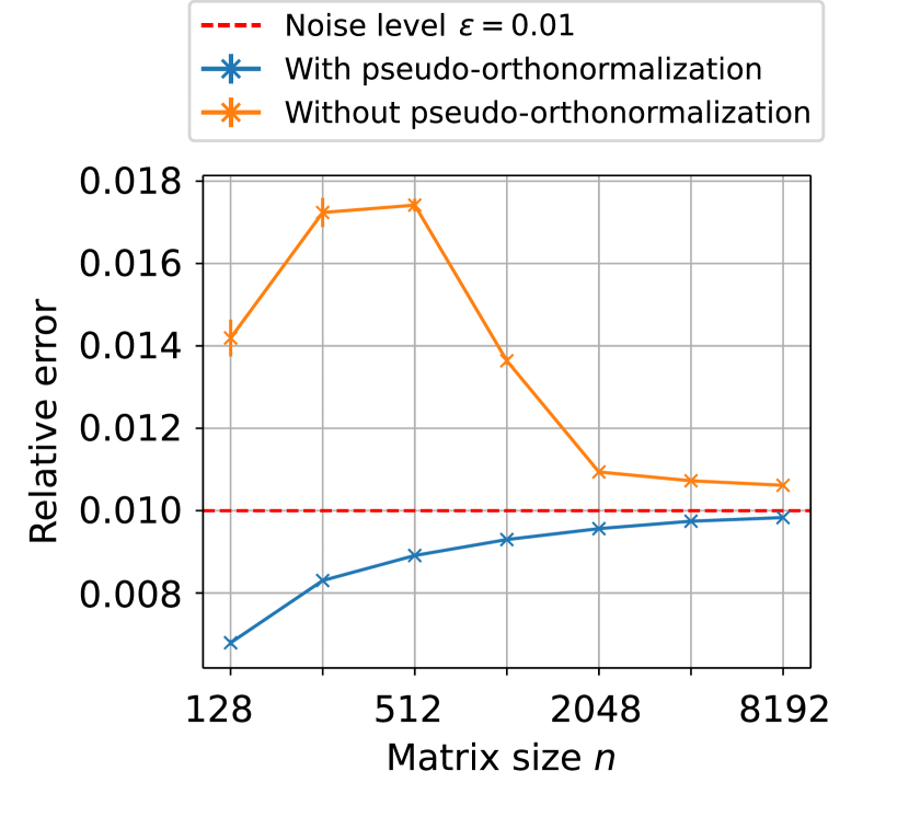
(a) $\epsilon=0.01$

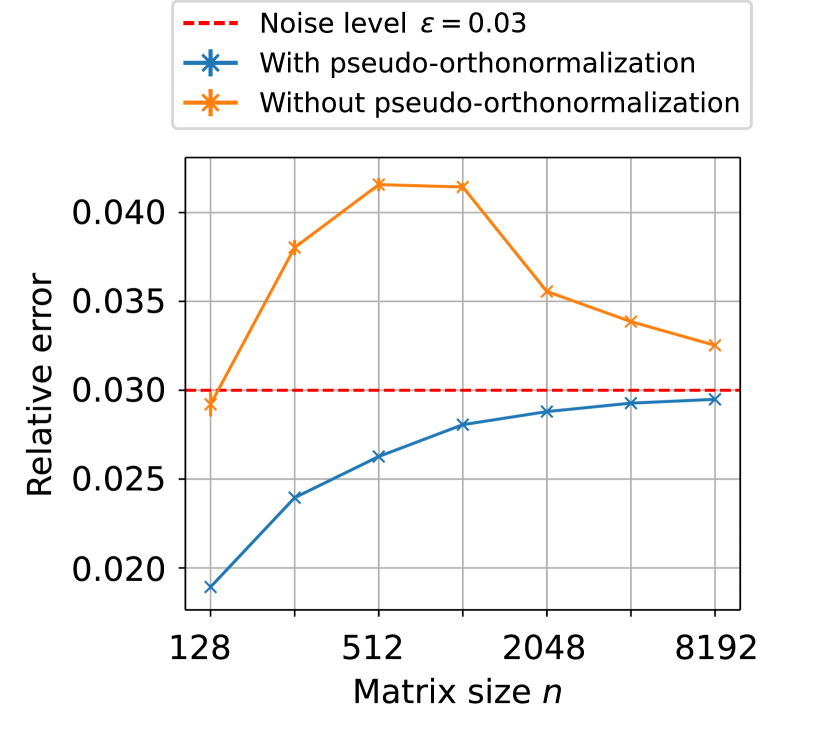
(b) $\epsilon=0.03$

(c) $\epsilon=0.1$

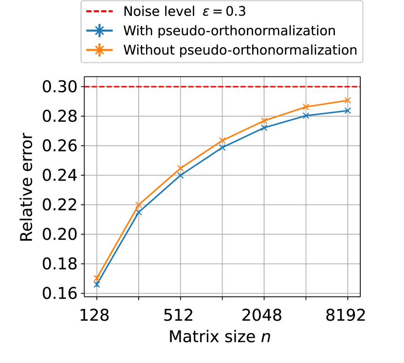
(d) $\epsilon=0.3$

Figure 8: Relative approximation errors vs. the matrix size $n$, for Algorithm 3 (without orthonormalization) and Algorithm 4 (with orthonormalization), for the instance of Problem (1) described in Section 8.2 with $r=4$. We show mean and standard deviation on the error bars over $10$ repetitions of the experiment.

References

- [1] S. Boyd and L. Vandenberghe. Convex Optimization. Cambridge University Press, USA, 2004.
- [2] E. Candes, L. Demanet, and L. Ying. A fast butterfly algorithm for the computation of fourier integral operators. Multiscale Modeling & Simulation, 7(4):1727–1750, 2009.
- [3] B. Chen, T. Dao, K. Liang, J. Yang, Z. Song, A. Rudra, and C. Ré. Pixelated butterfly: Simple and efficient sparse training for neural network models. In International Conference on Learning Representations, 2022.
- [4] T. Dao, B. Chen, N. S. Sohoni, A. D. Desai, M. Poli, J. Grogan, A. Liu, A. Rao, A. Rudra, and C. Ré. Monarch: Expressive structured matrices for efficient and accurate training. In International Conference on Machine Learning, pages 4690–4721. PMLR, 2022.
- [5] T. Dao, A. Gu, M. Eichhorn, A. Rudra, and C. Ré. Learning fast algorithms for linear transforms using butterfly factorizations. In International Conference on Machine Learning, pages 1517–1527. PMLR, 2019.
- [6] T. Dao, N. Sohoni, A. Gu, M. Eichhorn, A. Blonder, M. Leszczynski, A. Rudra, and C. Ré. Kaleidoscope: An efficient, learnable representation for all structured linear maps. In International Conference on Learning Representations, 2020.
- [7] L. Demanet and L. Ying. Fast wave computation via fourier integral operators. Mathematics of Computation, 81(279):1455–1486, 2012.
- [8] Alexey Dosovitskiy, Lucas Beyer, Alexander Kolesnikov, Dirk Weissenborn, Xiaohua Zhai, Thomas Unterthiner, Mostafa Dehghani, Matthias Minderer, Georg Heigold, Sylvain Gelly, Jakob Uszkoreit, and Neil Houlsby. An image is worth 16x16 words: Transformers for image recognition at scale. In International Conference on Learning Representations, 2021.
- [9] P. Duhamel and M. Vetterli. Fast fourier transforms: a tutorial review and a state of the art. Signal processing, 19(4):259–299, 1990.
- [10] C. Eckart and G. Young. The approximation of one matrix by another of lower rank. Psychometrika, 1(3):211–218, 1936.
- [11] N. Engheta, W. D. Murphy, V. Rokhlin, and M. S. Vassiliou. The fast multipole method (FMM) for electromagnetic scattering problems. IEEE Transactions on Antennas and Propagation, 40(6):634–641, 1992.
- [12] G. H. Golub and C. F. Van Loan. Matrix Computations. The Johns Hopkins University Press, third edition, 1996.
- [13] A. Gonon, L. Zheng, P. Carrivain, and Q.-T. Le. Fast inference with kronecker-sparse matrices. arXiv preprint arXiv:2405.15013, 2024.
- [14] H. Guo, Y. Liu, J. Hu, and E. Michielssen. A butterfly-based direct integral-equation solver using hierarchical lu factorization for analyzing scattering from electrically large conducting objects. IEEE Transactions on Antennas and Propagation, 65(9):4742–4750, 2017.
- [15] W. Hackbusch. Hierarchical matrices: Algorithms and analysis. Springer, 2015.
- [16] N. Halko, P. G. Martinsson, and J. A. Tropp. Finding structure with randomness: Probabilistic algorithms for constructing approximate matrix decompositions. SIAM Review, 53(2):217–288, 2011.
- [17] D. P. Kingma and J. Ba. Adam: A method for stochastic optimization. In International Conference on Learning Representations, 2015.
- [18] Q.-T. Le, E. Riccietti, and R. Gribonval. Spurious valleys, NP-hardness, and tractability of sparse matrix factorization with fixed support. SIAM Journal on Matrix Analysis and Applications, 2022.
- [19] Q.-T. Le, L. Zheng, R. Gribonval, and E. Riccietti. Code for reproducible research - Butterfly factorization with error guarantees, 2024. https://inria.hal.science/hal-04720713.
- [20] Q.-T. Le, L. Zheng, E. Riccietti, and R. Gribonval. Fast learning of fast transforms, with guarantees. In IEEE International Conference on Acoustics, Speech and Signal Processing, 2022.
- [21] L. Le Magoarou and R. Gribonval. Flexible multilayer sparse approximations of matrices and applications. IEEE Journal of Selected Topics in Signal Processing, 10(4):688–700, 2016.
- [22] Y. Li and H. Yang. Interpolative butterfly factorization. SIAM Journal on Scientific Computing, 39(2):A503–A531, 2017.
- [23] Y. Li, H. Yang, E. R. Martin, K. L. Ho, and L. Ying. Butterfly factorization. Multiscale Modeling & Simulation, 13(2):714–732, 2015.
- [24] Y. Li, H. Yang, and L. Ying. A multiscale butterfly algorithm for multidimensional fourier integral operators. Multiscale Modeling & Simulation, 13(2):614–631, 2015.
- [25] Y. Li, H. Yang, and L. Ying. Multidimensional butterfly factorization. Applied and Computational Harmonic Analysis, 44(3):737–758, 2018.
- [26] E. Liberty, F. Woolfe, P.-G. Martinsson, V. Rokhlin, and M. Tygert. Randomized algorithms for the low-rank approximation of matrices. Proceedings of the National Academy of Sciences, 104(51):20167–20172, 2007.
- [27] R. Lin, J. Ran, K. H. Chiu, G. Chesi, and N. Wong. Deformable butterfly: A highly structured and sparse linear transform. In Advances in Neural Information Processing Systems, volume 34, pages 16145–16157, 2021.
- [28] D. C. Liu and J. Nocedal. On the limited memory BFGS method for large scale optimization. Mathematical programming, 45(1-3):503–528, 1989.
- [29] Y. Liu, X. Xing, H. Guo, E. Michielssen, P. Ghysels, and X. S. Li. Butterfly factorization via randomized matrix-vector multiplications. SIAM Journal on Scientific Computing, 43(2):A883–A907, 2021.
- [30] E. Michielssen and A. Boag. Multilevel evaluation of electromagnetic fields for the rapid solution of scattering problems. Microwave and Optical Technology Letters, 7(17):790–795, 1994.
- [31] E. Michielssen and A. Boag. A multilevel matrix decomposition algorithm for analyzing scattering from large structures. IEEE Transactions on Antennas and Propagation, 44(8):1086–1093, 1996.
- [32] M. Munkhoeva, Y. Kapushev, E. Burnaev, and I. Oseledets. Quadrature-based features for kernel approximation. In Advances in neural information processing systems, 2018.
- [33] M. O’Neil. A new class of analysis-based fast transforms. Yale University, 2007.
- [34] M. O’Neil, F. Woolfe, and V. Rokhlin. An algorithm for the rapid evaluation of special function transforms. Applied and Computational Harmonic Analysis, 28(2):203–226, 2010.
- [35] I. V. Oseledets. Tensor-train decomposition. SIAM Journal on Scientific Computing, 33(5):2295–2317, 2011.
- [36] D. S. Parker. Random butterfly transformations with applications in computational linear algebra. UCLA Computer Science Department, 1995.
- [37] E. Quemener and M. Corvellec. Sidus—the solution for extreme deduplication of an operating system. Linux Journal, 2013(235):3, 2013.
- [38] C M Rader. Discrete Fourier transforms when the number of data samples is prime. Proceedings of the IEEE, 56:1107–1108, 1968.
- [39] S.-K. Shekofteh, C. Alles, and H. Fröning. Reducing memory requirements for the ipu using butterfly factorizations. In Proceedings of the SC’23 Workshops of The International Conference on High Performance Computing, Network, Storage, and Analysis, pages 1255–1263, 2023.
- [40] M. Tygert. Fast algorithms for spherical harmonic expansions, III. Journal of Computational Physics, 229(18):6181–6192, 2010.
- [41] Z. Yang, M. Moczulski, M. Denil, N. De Freitas, A. Smola, L. Song, and Z. Wang. Deep fried convnets. In Proceedings of the IEEE International Conference on Computer Vision, pages 1476–1483, 2015.
- [42] L. Ying. Sparse fourier transform via butterfly algorithm. SIAM Journal on Scientific Computing, 31(3):1678–1694, 2009.
- [43] L. Zheng, G. Puy, E. Riccietti, P. Pérez, and R. Gribonval. Butterfly factorization by algorithmic identification of rank-one blocks. arXiv preprint arXiv:2307.00820, 2023.
- [44] L. Zheng, E. Riccietti, and R. Gribonval. Efficient identification of butterfly sparse matrix factorizations. SIAM Journal on Mathematics of Data Science, 5(1):22–49, 2023.