medial quandles’s capability of detecting causality and properties of their coloring on certain links and knots

Abstract

I investigated the capability of medial quandle, quandle whose operation satisfying that $(a_{1}*b_{1})*(a_{2}*b_{2})=(a_{1}*a_{2})*(b_{1}*b_{2})$, to detect causality in (2+1)-dimensional globally hyperbolic spacetime by determining if they can distinguished the connected sum of two Hopf links from an infinite series of relevant three-component links constructed by Allen and Swenberg in 2020, who suggested that any link invariant must be able to distinguish those links for them to detect causality in the given setting. I show that these quandles fail to do so as long as $a\sim b\Leftrightarrow a*b=a$ defines an equivalence relation. The Alexander quandles is an example that this result can apply to. Inspired by this result, I also derived a generalized theorem about the coloring of medial quandles on a specific type of tangles, which help to determine whether this quandles can distinguish between a wider range of knots and links or not.

1 Introduction

Mathematical knots are embeddings of circles into 3-dimension Euclidean space. Two knots are equivalent only if they can be transformed to each other via a series of Reidemeister moves. A Link is a collection of knots that are intertwined together. A knot or link invariant is a function that assign same value to equivalent knots/links, which require it to be preserved under all Reidemeister moves. Using link invariant to distinguish link has been shown to relates detection of causality in spacetime with the following work from former researchers:

Let $X$ be a $(2+1)$-dimensional globally hyperbolic spacetime with Cauchy surface $\sum$ homomorphic to $\mathbb{R}^{2}$. Chernov and Nemirovski[1] proved the Low conjecture[2], which state that as long as $\sum$ is not homomorphic to $S^{2}$ or $\mathbb{R}p^{2}$, then two events $x,y\in X$ are causally related if and only if their skies $S_{x}\cup S_{y}$ are topologically linked. Two causally unrelated points in spacetime give a link isotopic to the connected sum of two Hopf link, denoted as $L_{2H}$ in this paper. This result gave rise to the possibility that the causality of two events in their skies can be detected by link invariants.

Allen and Swenberg[3] investigate the natural question that whether $S_{x}$ and $S_{y}$, and thus the causality, can be detected by link invariant. If there exist a three component link consists of one unknot and other two individually deformable to the longitudes of the solid torus $S^{1}\times R^{2}$ whose link invariant is the same as $L_{2H}$, then it is said that the link invariant can not completely determine causality in $X$. They showed that Conway-polynomial cannot detect causality in that space time, as there exist a infinite family of three-components two-sky-link link (Allen-Swenberg links) that can not be distinguished with the connected sum of two Hopf links by Conway polynomial.

This paper is organized as following: Section 2 introduced link invariant generated by quandle, an algebraic structure, and specifically for medial quandle. In section 3-4, this paper investigate the capability of medial quandle for distinguishing $L_{2H}$ and Allen-Swenberg links. This part eventually show that as long as the relation define on a medial quandle by $a~{}b\Leftrightarrow a*b=a$ is an equivalence relation, then it cannot distinguish $L_{2H}$ and any of Allen-Swenberg link in the series, thus fail to capture causality in the spacetime. Since Alexander quandles satisfy the restriction on qunadle in this result, one application of this result is that all Alexander quandle fail to detect causality in the given spacetime. Inspired by a lemma discovered in section 4, section 5 and 6 define an infinite family of tangles which are then proved to possess an interesting property under the coloring of medial quandle. This property helps to determine medial quandle’s coloring on a wider range of knots and links, and some applications are presented in section 7.

2 Mathematical background

definition 2.1: quandle

A quandle $Q(*)$ a set $Q$ equipped with a binary operation $*:(x,y)\to x*y$ such that the operation satisfy the following axioms, $\forall x,y,z\in Q:$
1. $x*x=x$
2. There exist an unique $q\in Q$ such that $q*y=x$. We can then define the inverse operation $*^{-1}$ as $x*^{-1}y=q$.
3. $(x*y)*z=(x*z)*(y*z)$

definition 2.2: quandle homomorphism

Given two quandle $A(*)$ and $B(\times)$, a homomorphism from $A(*)$ to $B(\times)$, $f\in Hom(A(*),B(\times))$, is a function $f:A\to B$ such that $f(x*y)=f(x)\times f(y)~{}\forall x,y\in A$.

definition 2.3 fundamental quandle of a link

For an oriented knot or link diagram with arc-set $L$, its fundamental quandle $Q(L,*)$ is the quandle on $L$ with quandle operation defined by crossing relations given by each crossing in the link diagram in the following way:

Theorem 2.1

The fundamental quandle is a link variant.
Miller[4] proved this by showing that quandle axioms are motivated by the Reide- meister moves in such a way that the fundamental quandle is locally invariant.

definition 2.4 quandle coloring invariant

For a link $L$ with its fundamental quanlde $Q(L,*)$ and a finite quandle $X(\times)$, the coloring space is set of all homomorphisms from $Q(L,*)$ to $X(\times)$, $Hom(Q(L,*),X(\times))$. We say an element in the space is a coloring on the link by quandle $X$. It can be regarded as a way of assigning an element in $X$ to each arc in $L$ such that those elements satisfy the crossing relations defined in $L$ but with the quandle operation in $X(\times)$.
The quandle coloring invariant is $|Hom(Q(L,*),X(\times))|$, the cardinality of coloring space.
Remark: The coloring space from a finite quandle $X$ on any links or knots $Q(L)$ always contains the set $C_{T}=\{f:Q(L)\to X,~{}a\to x~{}|~{}x\in X\}$, namely, the set of constant function from $Q(L)$ to $x$, where $|C_{T}|=|X|$. An element in $C_{T}$ is called the trivial coloring, sending every arcs in the link or knot to the same element in the quandle.

definition 2.5: enhanced coloring invariant

Defined by Nelson[6], using the same setting in definition 2.4, the enhanced coloring invariant is a polynomial in $q$ assign to the coloring space:

$$\Phi(L,X)=\sum_{f\in Hom(Q(L),X(\times)}q^{|IM(f)|}$$

This enhanced link invariant contains strictly more information then the quandle coloring invariant defined in 2.4.

definition 2.6 medial quandle

Medial quandle is the type of quandle $Q(*)$ such that $\forall x_{1},y_{2},x_{2},y_{2}\in Q$, they satisfy that $(x_{1}*y_{2})*(x_{2}*y_{2})=(x_{1}*x_{2})*(y_{1}*y_{2})$. Let $*^{-1}$ denote its inverse operation. It can be proved that a medial quandle satisfies the following 9 properties, for all $x,y,z,x_{1},x_{2},y_{1},y_{2}\in Q$:

$x*(y*z)=(x*x)*(y*z)=(x*y)*(x*z)~{}(1)$
$[(x_{1}*^{-1}y_{1})*(x_{2}*^{-1}y_{2})]*(y_{1}*y_{2})=[(x_{1}*^{-1}y_{1})*y_{1}]*[(x_{2}*^{-1}y_{2}*y_{2})]=x_{1}*x_{2}\to(x_{1}*^{-1}y_{1})*(x_{2}*^{-1}y_{2})=(x_{1}*x_{2})*^{-1}(y_{1}*y_{2})~{}(2)$
$(2)$ implies $x*^{-1}(y*z)=(x*x)*^{-1}(y*z)=(x*^{-1}y)*(x*^{-1}z)~{}(3)$, and
$[(x_{1}*^{-1}y_{1})*^{-1}(x_{2}*^{-1}y_{2})]*(y_{1}*^{-1}y_{2})=_{(2)}x_{1}*^{-1}x_{2}\to$
$(x_{1}*^{-1}y_{1})*^{-1}(x_{2}*^{-1}y_{2})=(x_{1}*^{-1}x_{2})*^{-1}(y_{1}*^{-1}y_{2})~{}(4)$
$(x*^{-1}y)*^{-1}z=(x*^{-1}y)*^{-1}(z*^{-1}z)=(x*^{-1}z)*^{-1}(y*^{-1}z)~{}(5)$ $x*^{-1}(y*^{-1}z)=(x*^{-1}x)(y*^{-1}z)=(x*^{-1}y)*^{-1}(x*^{-1}z)~{}(6)$
$(x*^{-1}y)*z=(x*^{-1}y)*(z*^{-1}z)=(x*z)*^{-1}(y*z)~{}(7)$
$x*(y*^{-1}z)=(x*^{-1}x)*(y*^{-1}z)=(x*y)*^{-1}(x*z)~{}(8)$
$[(x*^{-1}z)*(y*^{-1}z)]*z=x*y\to$ $(x*y)*^{-1}z=(x*^{-1}z)*(y*^{-1}z)~{}(9)$ ( $(9)$ is true for all quandle)

Example 2.7: Alexander quandle

An Alexander quandle is a module $M$ over $\mathbb{Z}[t^{\pm}]$ under the the operation $a*b=ta+(1-t)b$. Since we need finite quandle for quandle coloring link invariant, we consider finite Alexnader quandle which is in the form $Q=\mathbb{Z}_{n}[t^{\pm}]/(h(t))$ where $h$ is a monic polynomial in $t$ (Nelson[5]). It is a medial quandle because $\forall a_{1},b_{1},a_{2},b_{2}\in Q$,
$(a_{1}*b_{1})*(a_{2}*b_{2})=(ta_{1}+(1-t)b_{1})*(ta_{2}+(1-t)b_{2})=(t^{2}a_{1}+t(1-t)b_{1})+(t(1-t)a_{2}+(1-t)^{2}b_{2})=(t^{2}a_{1}+t(1-t)a_{2})+(t(1-t)b_{1}+(1-t)^{2}b_{2})=(ta_{1}+(1-t)a_{2})*(tb_{1}+(1-t)b_{2})=(a_{1}*a_{2})*(b_{1}*b_{2})$.

2.1 Example: coloring on the trefoil knot

The trefoil knot (denoted as $k_{3}$) is the following:

The fundamental quandle of $k_{3}$ is in the form $Q(k_{3},\times)=\{a,b,c~{}:~{}c\times b=a,b\times a=c,a\times c=b\}$. Consider the quandle on set $\mathbb{Z}_{3}$ with operation $x*y=2x-y$. Then to derive the coloring space of this quandle on the trefoil knot is essentially solving this system of modulo equations: $\{2c-b=a,2b-a=c,2a-c=b~{}(mod~{}3)\}$. One can check that the solutions require that $a=b=c,a\in\mathbb{Z}_{3}$.
This means $Hom(Q(k_{3},\times),\mathbb{Z}_{3}(*))=\{(a\to 1,b\to 1,c\to 1),(a\to 2,b\to 2,c\to 2),(a\to 3,b\to 3,c\to 3)\}$. The coloring invariant from $\mathbb{Z}_{3}(*)$ on the trefoil knot is therefore $|~{}Hom(Q(k_{3},\times),\mathbb{Z}_{3}(*))~{}|=3$. All function has only 1 image, so the enhanced polynomial is $\Phi(k_{3},\mathbb{Z}_{3}(*))=3q^{1}$.

3 medial quandle & detecting causality

Allen and Swenberg[2] investigated whether there are link invariants can detect causality in $X$, a (2+1)-dimensional globally hyperbolic spacetime with a Cauchy surface $\sigma$ whose universal cover is homomorphic to $R^{2}$. They constructed an infinite series of three-component links (Allen-Swenberg links), and suggested that such link invariant needs to be able to distinguish between these links and connected sum of two Hopf ($L_{2H})$. (see figures of the links below). They found that Conway polynomial fail to do so. I would show the coloring invariant and its enhanced polynomial from any meidal quandle with $a\sim b\Leftrightarrow a*b=a$ defining an equivalence relation also can’t differentiate $L_{2H}$ from the Allen-Swenberg links.

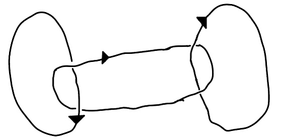
Figure 3.1: connected sum of two Hopf links,denoted by $L_{2H}$

The first Allen-Swenberg link in series, $A_{1}$ is

The nth Allen-Swenberg link, denoted by $A_{n}$, is form by duplicating the complex tangle in the middle component :

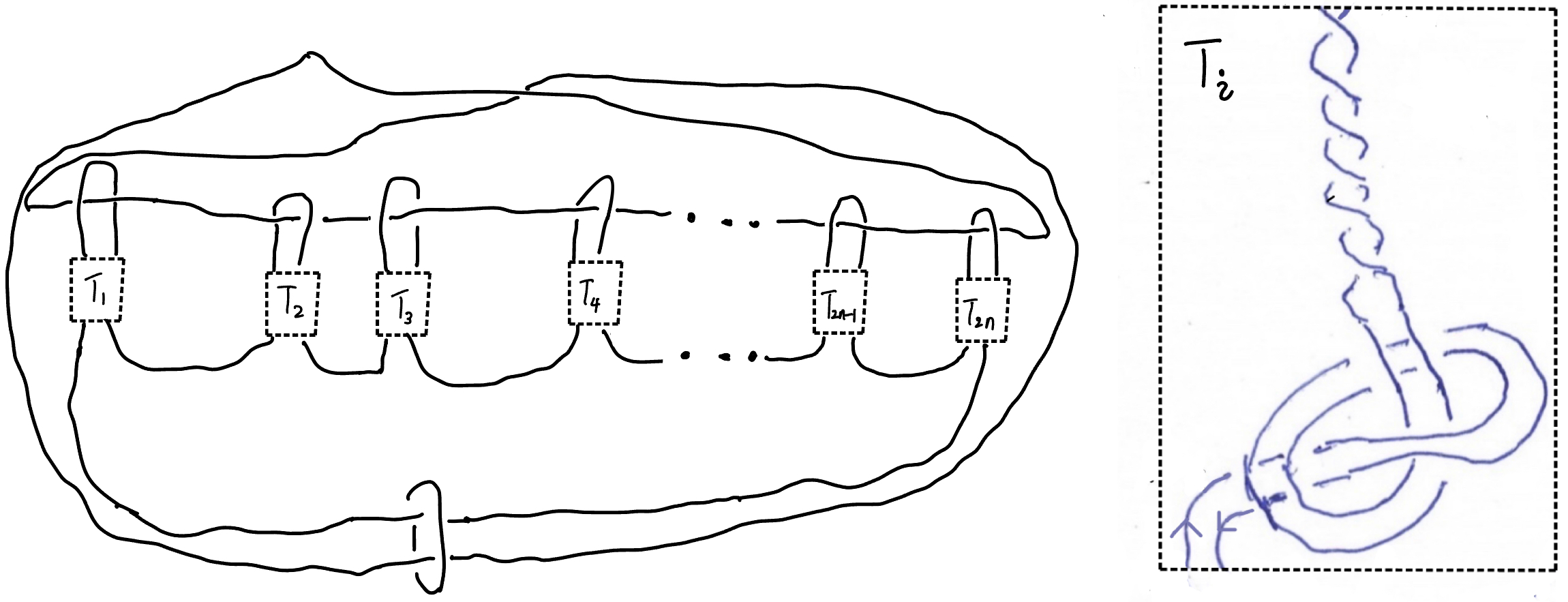
Figure 3.2: general Allen-Swenberg links $A_{n}$ and the tangle $T$ that consists of it

3.1 Proposition 3.1

Let $Q(*)$ be a medial quandle (definition 2.6) such that the relation $\sim$ on $Q$ defined by $a\sim b\Leftrightarrow a*b=a$ is an equivalence equation.
Let $C_{A_{i}}$ and $C_{H}$ denote the cardinality of the coloring space of the quandle on the ith Allen-Swenberg link and the connected sum of two Hopf links, respectively (i.e., $C_{A_{i}}=|Hom(A_{i},Q(*))|,~{}C_{H}=|Hom(L_{2H},Q(*))|$. Let $\Phi(A_{i},Q(*),\Phi(L_{2H},Q(*))$ denote the enhanced coloring polynomial(definition 2.5) of the two links under the coloring by $Q(*)$, respectively. Then
$C_{A_{i}}=C_{H}$ and $\Phi(A_{i},Q(*))=\Phi(L_{2H},Q(*)),~{}\forall i\in\mathbb{Z}^{+}$.
This means any coloring invariant or its enhanced polynomial generated by medial quandle with the equivalence relation defined above is unable to distinguish between any of Allen-Swenberg links and the connected sum of Hopf link, therefore this type of medial quandles fail to detect causality in the given setting.

Example: Alexander quandle

All finite Alexander quandle defined in section 2.7 satisfy the property of $Q(*)$ defined above. Section 2.7 show it is medial. The relation $\sim$ defined on a finite Alexander quandle $A=\mathbb{Z}_{n}[t^{\pm}]/(h(t))$ is
$a\sim b\Leftrightarrow a*b=a\Leftrightarrow ta+(1-t)b=a~{}(mod~{}h(t))$. This is equivalent to
$(t-1)a=(t-1)b~{}(mod~{}h(t))$, which is clearly an equivalence relation. So proposition 3.1 imply that Alexander quandle are unable to detect causality in the given spacetime.

4 Proof for proposition 3.1

First we prove some properties of medial quandle which will be used later. In some calculation process below, $=_{(i)}$ or $=_{k}$ means that the right side of the equation are derived by applying property $(i)$ in section 2.6 or property k in this section that is already proved. Let $Q(*)$ be a medial quandle. Then
1.$[(a*x)*^{-1}y]*z=[(a*z)*^{-1}y]*x,~{}\forall a,x,y,z\in Q$.
Proof :
$[(a*x)*^{-1}y]*z=_{(7)}[(a*x)*z]*^{-1}(y*z)=[(a*z)*(x*z)]*^{-1}(y*z)=_{(2)}[(a*z)*^{-1}y]*[(x*z)*^{-1}z]=[(a*z)*^{-1}y]*x$, as desired.

2. $[(a*^{-1}x)*y]*^{-1}z=[(a*^{-1}z)*y]*^{-1}x$.
Proof: A easy way to proof this is noticing that the original and inverse operation $*$ and $*^{-1}$ is completely symmetric in a medial quandle. This is because one can check that replacing all $*$ by $*^{-1}$ and all $*^{-1}$ by $*$ in any one of properties in section 2.6 gives another property that is also satisfied by $Q(*)$. So if an equation for operation in $Q(*)$ holds, than the equation derived by switching between all $*$ and $*^{-1}$ in the original equation is also valid. By doing it to 1 we get $[(a*^{-1}x)*y]*^{-1}z=[(a*^{-1}z)*y]*^{-1}x$, which is exactly 2, which completes the proof.

definition 4.1

For any $x,y\in Q$, define $f_{xy}:Q\to Q$ by $f_{xy}(q)=(q*^{-1}x)*y$.
Let $f_{x_{2}y_{2}}\circ f_{x_{1}y_{1}}(q):=f_{x_{2}y_{2}}(f_{x_{1}y_{1}}(q))$ denote the composition of two such function. Then $\forall x,y,a,b,q\in Q$,

4. $f_{xy}\circ f_{ab}=f_{ab}\circ f_{xy}$. Proof: $f_{xy}\circ f_{ab}(q)=[[(q*^{-1}a)*b]*^{-1}x]*y=_{1}[[(q*^{-1}x)*b]*^{-1}a]*y=_{2}[[(q*^{-1}x)*y]*^{-1}a]*b=f_{ab}\circ f_{xy}(q)$
5. $f_{1}\circ f_{2}\circ...\circ f_{k}=f_{1^{\prime}}\circ f_{2^{\prime}}\circ...\circ f_{k^{\prime}}$, where $\{i\}\to\{i^{\prime}\}$ is a permutation, and $f_{i}=f_{x_{i}y_{i}}$ for some $x_{i},y_{i}\in Q$.
Proof: every permutation can by derived by a series of transposition, and each transposition can be derived by a series of switch between adjacent element. It follows from 4 that switching between adjacent individual functions preserve the composited function, which complete this proof.

6. $f_{xy}(a*b)=f_{xy}(a)*f_{xy}(b)$ and $f_{xy}(a*^{-1}b)=f_{xy}(a)*^{-1}f_{xy}(b)$. Proof:
$f_{xy}(a*b)=[(a*b)*^{-1}x]*y=[(a^{-1}x)*(b*^{-1}x)]*y=[(a^{-1}x)*y]*[(b^{-1}x)*y]=f_{xy}(a)*f_{xy}(b)$, and
$f_{xy}(a*^{-1}b)=[(a*^{-1}b)*^{-1}x]*y=[(a*^{-1}x)*^{-1}(b*^{-1}x)]*y=[(a*^{-1}x)*y]*^{-1}[(b^{-1}x)*y]=f_{xy}(a)*^{-1}f_{xy}(b)$.

4.1 coloring on connected sum of two Hopf links

Let $Q(*)$ be a medial quandle such that the relation $\sim$ on $Q$ defined by $a\sim b\Leftrightarrow a*c=a$ is an equivalence equation. For the connected sum of two Hopf links, the system of equations associated to the coloring space comes from only 4 crossings, so it can be calculated relatively easily. Consider the following label by a valid coloring on $L_{2H}$ by $Q$:

The four crossing relation give the following requirements:
$t_{1}:$ $x*y_{1}=x$. Since $\sim$ is an equivalence equation, this imply $x\sim y_{1}\to y_{1}\sim x\to y_{1}*x=y_{1}$
$t_{2}:$ $y_{2}=y_{1}*x=y_{1}.$. So $y_{1}=y_{2}$
$t_{3}:$ $y_{1}=y_{2}*z\to y_{1}*z=y_{1}$, so $y_{1}\sim z$
The first three crossings generate the solution set $\{x,y_{1},y_{2},z\}=\{x,y,y,z\}$ with the condition that $x\sim y\sim z$ where $x,y,z\in Q$. It automatically satisfy the equation given by $t_{4}:$ $z*y_{2}=z$ because we have $y_{1}=y_{2}$ and $y_{1}\sim z$ which imply $z\sim y_{2}\to z*y_{2}=z$.

4.2 Lemma 1

Consider the following tangle as a subpart of the Allen-Swenberg link (called $T$ in section 3) , which I will call $L_{p}$.

Claim: when applying coloring from any medial quandle $Q(*)$, the system of equations with the operation from $Q(*)$ given by this subpart link diagram force $n=d$ and $m=e$.

4.3 proof of lemma 1

Firstly, notice that the following subpart of link diagram $L_{p^{\prime}}$ is mathematically the same as $L_{p}$ because they can transform to each other by only Reidemeister move type $III$:

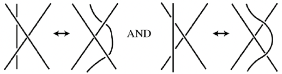
Figure 4.1: Reidemeister moves type $III$

transformation:

This mean it suffices to prove the the two pairs of exiting line segment of $L_{p}^{\prime}$ has the same value respectively.
Let $Q(*)$ be an arbitrary medial quandle. Let’s first analysis the coloring of $Q(*)$ on the following two structures, called structure ① and ②,respectively. In both structures by labeling 4 of the arcs exposed outside with $x,y,n,m$ representing some element in $Q(*)$, the other 4 out-exposed aces labeled by $x^{\prime},y^{\prime},n^{\prime},m^{\prime}$ can be expressed by a string of quandle operations between $x,y,n,m$. By using the properties of medial quandle given in section 2.6, these expressions can be further simplified to the form of some functions $f_{pq},~{}p,q\in\{x,y,n,m\}$ defined in definition 4.1 acting on one of $x,y,n,m$ The result is shown in the figure below and the calculation process is shown below.

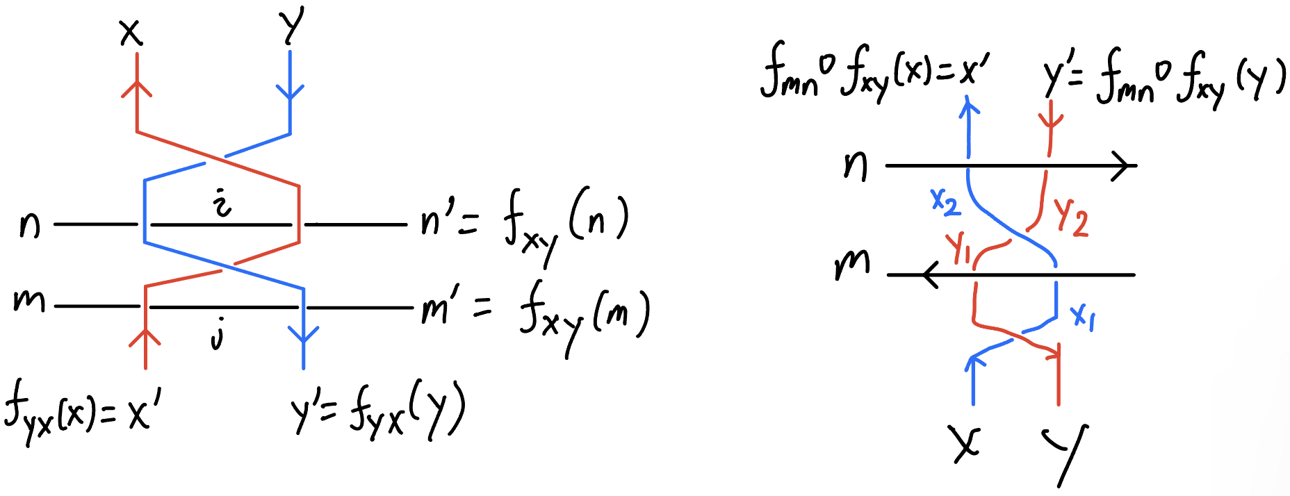
Figure 4.2: structure 1(left) and structure 2(right). Recall the definition of $f_{xy}$ in definition 4.1

For structure ①:
$y^{\prime}=y*x=(y*^{-1}y)*x=f_{yx}(y)$
$x^{\prime}=x*^{-1}y^{\prime}=x*^{-1}(y*x)=(x*^{-1}y)*(x*^{-1}x)=(x*^{-1}y)*x=f_{yx}(x)$
$n^{\prime}=i*^{-1}x=(n*y^{\prime})*^{-1}x=[n*(y*x)]*^{-1}x=[(n*^{-1}x)*[(y*x)*^{-1}x]]=(n*^{-1}x)*y=f_{xy}(n)$.
$m^{\prime}=j*y^{\prime}=(m*^{-1}x^{\prime})*(y^{\prime})=[m*^{-1}[(x*^{-1}y)*x]]*(y^{\prime})=(m*y^{\prime})*^{-1}[[(x*^{-1}y)*x]*y^{\prime}]=(m*y^{\prime})*^{-1}[[(x*^{-1}y)*x]*(y*x)]=[m*(y*x)]*^{-1}x=(m*^{-1}x)*[(y*x)*^{-1}x]=(m*^{-1}x)*y=f_{xy}(m)$.
For structure ②: $x_{1}=x*y~{}~{}x_{2}=x_{1}*^{-1}m~{}~{}y_{1}=y*^{-1}m~{}~{}y_{2}=y_{1}*^{-1}x_{2}$, so
$x^{\prime}=x_{2}*n=(x_{1}*^{-1}m)*n=[(x*y)*^{-1}m]*n=[[(x*^{-1}x)*y]*^{-1}m]*n=f_{mn}\circ f_{xy}(x)$
$y^{\prime}=y_{2}*n=(y_{1}*^{-1}x_{2})*n=[(y*^{-1}m)*^{-1}(x_{1}*^{-1}m)]*n=[(y*^{-1}x_{1})*^{-1}m]*n=[[y*^{-1}(x*y)]*^{-1}m]*n=[[(y*^{-1}x)*y]*^{-1}m]*n=f_{mn}\circ f_{xy}(y)$

Now we can view $L_{P^{\prime}}$ as the combination of two structures 1 and one structure 2:

By applying the calculation result in Figure 4.2 on the three structures 1 or 2 in above figure one by one, we have
$d=f_{ji}(j),~{}j=f_{m^{\prime}n^{\prime}}\circ f_{ba}(b),~{}b=f_{yx}(y),~{}y=f_{ij}(n^{\prime}),~{}n^{\prime}=f_{xy}(n)$. and
$e=f_{ji}(i),~{}i=f_{m^{\prime}n^{\prime}}\circ f_{ba}(a),~{}a=f_{yx}(x),~{}x=f_{ij}(m^{\prime}),~{}m^{\prime}=f_{xy}(m)$. In order to simplify the expression for $j$, notice that these equations gives $b=f_{yx}\circ f_{ij}(n^{\prime}),~{}a=f_{yx}\circ f_{ij}(m^{\prime})$. Let $g:=f_{yx}\circ f_{ij}$. By property 5, $g((p*q))=g(p)*g(q),~{}g((p*^{-1}q))=g(p)*^{-1}(q)~{}~{}\forall p,q\in Q$. So $j=f_{m^{\prime}n^{\prime}}\circ f_{ba}(b)=f_{m^{\prime}n^{\prime}}[(g(n^{\prime})*^{-1}g(n^{\prime}))*g(m^{\prime})]=f_{m^{\prime}n^{\prime}}(g(n^{\prime}*m^{\prime}))=g(f_{m^{\prime}n^{\prime}}(n^{\prime}*m^{\prime}))=g([(n^{\prime}*m^{\prime})*^{-1}m^{\prime}]*n)=g(n^{\prime})=b$.
Similarly since $i=f_{m^{\prime}n^{\prime}}\circ f_{ba}(a)$, using similar method we can get $i=a$.
Plugging in $j=b,~{}i=a$, the above equations gives $d=f_{ji}\circ f_{yx}\circ f_{ij}\circ f_{xy}(n)$ and $e=f_{ji}\circ f_{yx}\circ f_{ij}\circ f_{xy}(m)$.
Note that $f_{vw}\circ f_{vw}$ is the identity function for all $v,w\in Q(*)$ because $\forall q\in Q(*),$
$f_{vw}\circ f_{vw}(q)=[[(q*^{-1}v)*w]*^{-1}w]*v=(q*^{-1}v)*v=q$. So combining these equations and rearranging each individual functions which property 5 (see at the start of section 4) allows, we have
$d=f_{ji}\circ f_{ij}\circ f_{yx}\circ f_{xy}(n)=f_{ji}\circ f_{ij}(n)=n$ and $e=f_{ji}\circ f_{ij}\circ f_{yx}\circ f_{xy}(m)=f_{ji}\circ f_{ij}(m)=m$.
This show under a valid coloring from any distributive quandle,the labeled arcs must satisfy the relation $d=n,e=m$, which complete the proof.

4.4 coloring on the first Allen-Swenberg link

Proposition 4.4

Let $Q(*)$ be a medial quandle such that the relation $\sim$ on $Q$ defined by $a\sim b\Leftrightarrow a*c=a$ is an equivalence equation. Then referring to figure 4.3, its coloring space on the first Allen-Swenberg link $A_{1}$ is the solution set $\{x1=x2=x3=x4=c_{1},y1=y2=c_{2},~{}others=c_{3}\}$, where $c_{1},c_{2},c_{3}\in Q$ with the condition that $c_{1}\sim c_{2}\sim c_{3}$ $"others"$ refer to all line segment in figure 3 other than $x1,x2,x2,x4,y1,y2$.

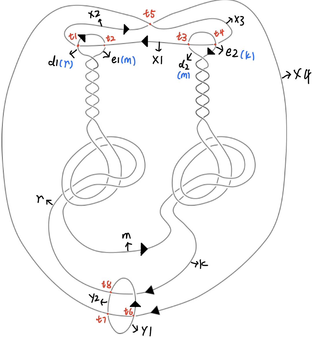
Figure 4.3: $A_{1}$ with orientation. Some arc and crossing are labeled for writing the proof

Proof for proposition 4.4

Lemma 1 requires that $d_{1}=r,e_{1}=d_{2}=m,e_{2}=k.$ The crossing relations given by the 5 crossings on the top in Figure 4.3 gives:
$t_{2}\&t_{3}:$ $r=m*^{-1}x_{1}=k$. $t_{1}\&t_{4}:$ $x_{2}=x_{1}*r=x_{1}*k=x_{3}$. $t_{5}:$ $x_{4}=x_{2}*x_{3}=x_{3}*x_{3}=x_{3}$. So we can let $x:=x_{4}=x_{2}*x_{3}=x_{3}*x_{3}=x_{3}$. The 3 crossings at the bottom give:
$t_{6}:$ $x*y_{1}=x\to x\sim y_{1}\to y_{1}\sim x_{1}.$
$t_{7}:$ $y_{2}=y_{1}*^{-1}x_{1}$. Since $y_{1}\sim x_{1},~{}y_{1}*x=y_{1}\to y_{1}=x*^{-1}y_{1}$, so $y_{2}=y_{1}$. .
$t_{8}:$ $y_{1}*r=y_{2}\to y_{1}*r=y_{1}\to y_{1}\sim r$. Getting back to $t_{1}:$, we have $x_{1}=x*^{-1}r.$ Since by calculation above we have $y_{1}\sim r,~{}x\sim y_{1}$, so $x\sim r\to x*r=x\to x=x*^{-1}r$. So $x_{1}=x*^{-1}r=x$.
By $t_{2}:$, Since $x\sim r$ imply $r\sim x$, we have $m=r*x_{1}=r*x=r$.
Since $r=k,r=m$, we have $m=k=r$.
Since the modulo equations generated by existing crossing already required $r=m=k$, the complex middle parts of strands degenerated and became equivalent as the unknot:

This means that all variable in the middle part has to have the same value, which is $m$. Let $y:=y_{1},~{}z:=m$. Combining the results derived above that $x_{1}=x_{2}=x_{3}=x_{4},y_{1}=y_{2}$, $x\sim y_{1}\sim r=m$, the solution set for coloring from $Q(*)$ to $A_{1}$ should be $\{x1=x2=x3=x4=x,y1=y2=y,~{}others(the~{}middle~{}2~{}L_{p}~{}structures)=z\}$ with condition that $x\sim y\sim z$.

4.5 coloring on general Allen-Swenberg links

In the oriented $A_{k}$ diagram, we can apply lemma 1 to label all arcs in the middle component outside each $T_{i}$ by $m_{j}$ where $0\geq j\leq 2n$:

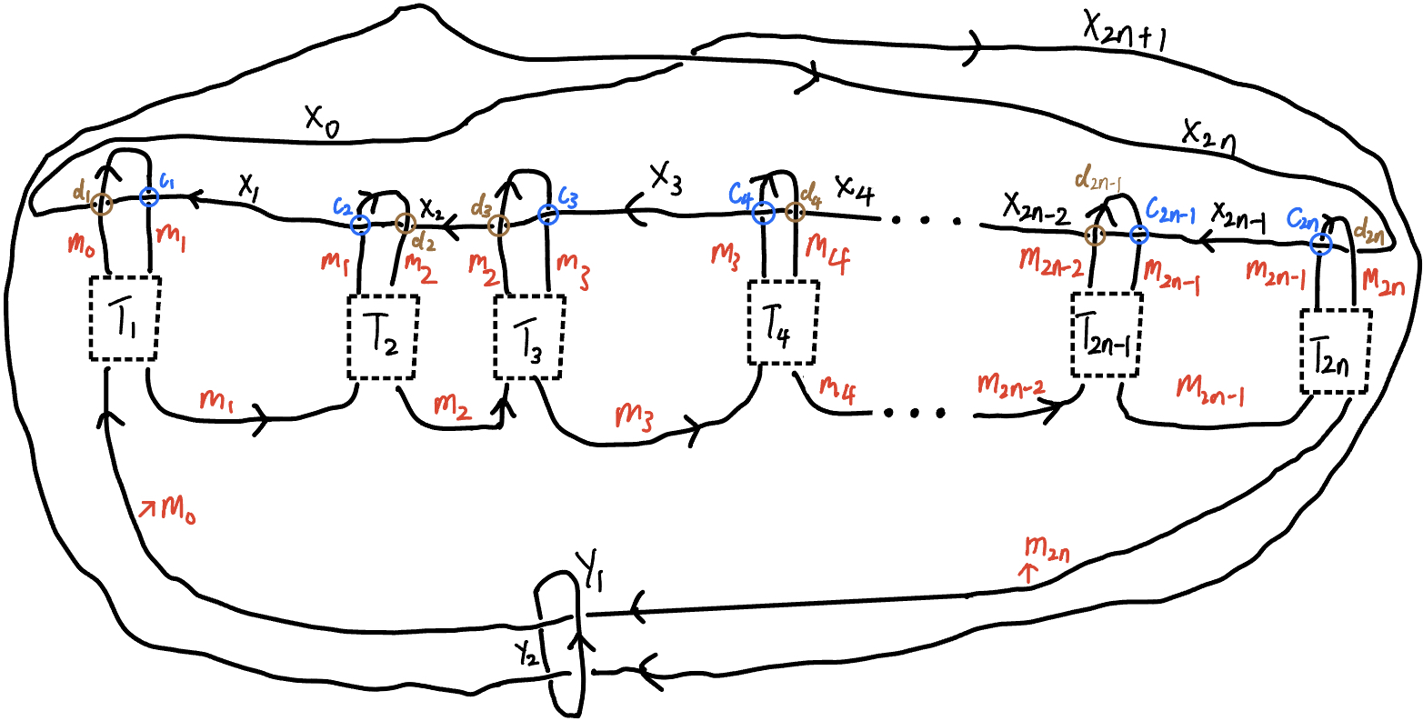
Figure 4.4: $A_{n}$ with orientation and partial labels

Proposition 4.5

The coloring space of $Q(*)$ on $A_{n}$ is the solution set $\{x_{i}=c_{1},y_{1}=y_{2}=c_{2},others=c_{3}~{}|~{}c_{1},c_{2},c_{3}\in Q,~{}c_{1}\sim c_{2}\sim c_{3}\}$. $others$ refer to all $m_{i}$ and all arcs in each $T_{j}$.

Proof for proposition 4.5

$\forall i\in\{1,3,...,2n-1\}$, the pair of crossings $c_{i}$ and $c_{i+1}$ imply $m_{i-1}=m_{i}*^{-1}x_{i}=m_{i+1}$. Therefore we have $m_{0}=m_{2},m_{2}=m_{4},...$, which gives $m_{0}=m_{2}=m_{4}=...=m_{2n}$ ($I$). With this result, the pair of crossings $d_{i}$ and $d_{i+1}$ give $x_{i-1}=x_{i}*m_{i-1}=x_{i}*m_{i+1}=x_{i+1}$, so similarly we have $x_{0}=x_{2}=x_{4}=...=x_{2n}$ ($II$), particularly, $x_{0}=x_{2n}$. For each $j\in\{2,4,...,2n\}$,the crossing $d_{j}$ gives $x_{j-1}=x_{j}*^{-1}m_{j}$. Combining ($I$) and ($II$), we have $x_{j}*^{-1}m_{j}$ is the same for all $j$,so $x_{j+1}$ is also all the same, namely $x_{1}=x_{3}=...=x_{2n-1}$ ($III$)
By using the fact that relation $\sim$ on $Q$ defined by $a\sim b\Leftrightarrow a*b=a$ is an equivalence relation, we can then repeat the process in section 4.4 of calculating the crossing equations given by ${\color[rgb]{1,0,0}t_{5},t_{6},t_{7},t_{8}}$ in figure 4.4 to derived that $x_{0}=x_{2n}=x_{2n+1}$, $y_{1}=y_{2}$(1), and $m_{0}=m_{2n}$, and $x_{0}\sim y_{1}\sim m_{0}$. Combining this with ($I$), we have $m_{i}\sim y_{1}\sim x_{0}$(2) for all even $i$.
By (2), $x_{0}\sim m_{0}$ so $x_{0}*m_{0}=x_{0}$, so crossing $d_{1}$ gives $x_{1}=x_{0}*^{-1}m_{0}=x_{0}$. Combining with $(II)$ and $(III)$, we have $x_{i}=x_{j}~{}\forall i,j\in\{1,2,...,2n+1\}$(3). For each odd $j$, $j-1$ is even, so by (2) and (3) $m_{j-1}\sim x_{j}$, so the crossing $c_{j}$ gives $m_{j}=m_{j-1}*x_{j}=m_{j-1}$. This means $m_{0}=m_{1},m_{2}=m_{4},...,m_{2n-2}=m_{2n-1}$, and by ($I$), we also have $m_{2n-1}=m_{2n}$.
When the system of crossing relations given by all $T_{i}$ are added with the equations $\{m_{0}=m_{1},m_{2}=m_{4},...,m_{2n-1}=m_{2n}\}$ we just derived, this given the system of crossing relations generated by the knot formed by connecting all $m_{i}$ and $m_{i+1}$ together for $i\in\{0,2,...,2n\}$. This knot is obviously equivalent to an unknot, so the middle complex component in $A_{k}$ degenerate to an unknot under the coloring by $Q(*)$, which means all $m_{i}$ and all arcs in $T_{i}$ must be colored to be the same element, so we can say they also equal to $m_{0}$. This result along with (1), (2) and (3) complete the proof of proposition 4.5.

4.6 summarization

By section 4.1,4.4 and 4.5, if $Q(*)$ is a medial quandle such that the relation $\sim$ on $Q$ defined by $a\sim b\Leftrightarrow a*c=a$ is an equivalence equation, the solutions sets correspond to the coloring space for both connected sum of two Hopf links $L_{2H}$ and general Allen-Swenberg links $A_{k}$ are in the form $\{x=c_{1},y=c_{2},z=c_{3}~{}\forall x\in X,y\in Y,z\in Z~{}|~{}c_{1}\sim c_{2}\sim c_{3}\in Q(*)\}$, where $X,Y,Z$ is a partition of the correspond arcs set of the link $Q(L)$. This means the coloring space both $L_{2H}$ and any $A_{k}$ should be $\{f:Q(L)\to Q(*)~{}|~{}f(X)=\{c_{1}\},f(Y)=\{c_{2}\},f(Z)=\{c_{3}\},c_{1}\sim c_{2}\sim c_{3}\}$.
Let $X,Y,Z$ be the partition for $L_{2H}$ and $X^{\prime},Y^{\prime},Z^{\prime}$ be the partition for $A_{k}$ respectively in their solution sets defined above. I would first show that there exist a bijection function $f:Hom(L_{2H},Q(*))\to Hom(A_{k},Q(*))$. Let $h\in Hom(L_{2H},Q(*))$ be arbitrary. By the discussion above, $h$ is defined by $h(X)=\{c_{1}\},h(Y)=\{c_{2}\},f(Z)=\{c_{3}\}$, for some $c_{1},c_{2},c_{3}\in Q(*)$ such that $c_{1}\sim c_{2}\sim c_{3}$. So we can define $f$ by defining $f(h):A_{k}\to Q$ to be:
$f(h)(X^{\prime})=\{c_{1}\},f(h)(Y^{\prime})=\{c_{2}\},f(h)(Z^{\prime})=\{c_{3}\}$. $f$ is obviously bijective, which shows $C_{A_{k}}=C_{2H}$. Since $Im(h)=\{c_{1},c_{2},c_{3}\}=Im(f(h))$, this function also preserve the cardinality of the image of the input function.
To show that $\Phi(A_{i},Q(*))=\Phi(L_{2H},Q(*))$ is equivalent of showing that $\forall i\in\{1,2,3\}$,
$|\{h\in Hom(L_{2H},Q(*)):~{}|Im(h)|=i\}|=|\{g\in Hom(A_{k},Q(*)):~{}|Im(g)|=i\}|$. It suffices to show there is a bijective map between this two set. Obviously, the function $f$ we previously defined restricted to the given domain, $f_{|\{h\in Hom(L_{2H},Q(*))~{}|~{}|Im(h)|=i\}}$, is bijective and indeed a function between this two sets. Therefore, $\Phi(A_{i},Q(*))=\Phi(L_{2H},Q(*))$.
This completes the proof for Proposition 3.1.

5 a more general property of medial quandle’s coloring on link and knot

This section generalizes Lemma 1 in section 4.2 to speak about a wider range of strand diagrams (formally defined below in definition 5.1) that share some common features with $L_{p}$ in the figure in section 4.2. It will focus on the property of the coloring from medial quandle (definition 2.6) to this type of strand diagrams. This property will be proposed in theorem 5.1, which can be use to determine whether medial quandle can distinguish some types of links and knots. Some applications will be discussed in section 7.

Definition 5.1

: Analogy to tangle, we define an open-strand diagram be a planar diagram that can be formed by cutting off two different arcs in a knot diagram. An oriented strand diagram is generated from an oriented knot diagram by the same process. If there is only one arc in a knot diagram,i.e, an unknot, this definition then does not make sense, so we specially defined two separated line segment with opposite orientation be also an oriented open-strand diagram, called the trivial open-strand. It can be seem as the diagram formed by cutting off an unknot(a circle) diagram in two difference spots. An open-strand diagram can be considered as two line segments intertwining with each other. Figure 5.1 shows two examples, one is a tangle and the other is not.

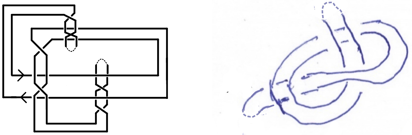
Figure 5.1: examples of open-strand diagram. The dotted curves represent that spots that are cut off in the knots that generate them.

Since the motivation of this definition is to study the quandle coloring on the arc-set of these diagrams, two open-strand diagrams are considered to be the same if they can be transformed to each other by Reidemeister moves. This, however, does not mean that two open-strand diagrams generated by two knots that are equivalent to each other are equivalent. The two examples in figure 5.1 are both generated by knots equivalent to unknot, but the open-strand diagran are considered to be different here.

Definition 5.2 the paths for arcs in strand diagram

:
Imagine putting a ball on an arc in an open-strand diagram that has a free end, and let the ball travel through the line in the direction of the other end,without stopping when passing below a crossing, until it reach another ending arc. I want to define the path for the starting arc to be a set containing of all arcs that is covered by this motion in order. The formal definition is the following:
Let $L$ be an non-trivial open-strand diagram (this imply the knot that generated it contains at least 3 arcs). Define a new symmetric crossing relation $\sim$ on $S_{L}$, the arcs-set of $L$ to be that $x\sim y$ and $y\sim x$ if they are connected by the arcs that passes above in a crossing :

Let $E\subseteq S_{L}$ denote the set of arcs in $L$ that has one end that does not intersect with any other arcs in the strand diagram. It is easy to see by definition that $|E|=4$. If we defined $\sim$ on a knot with arc set $K$ that contains at least 3 arc, then we see that $\forall x\in K$, $x\nsim x$, and there exist exactly two arcs $a,b\in K$ such that $a\sim x,b\sim x$. Also, it is impossible to exist distinct arcs $x_{1},x_{2},...x_{k}$ in $K$ such that $x_{1}\sim x_{2},x_{2}\sim x_{3},...,x_{k-1}\sim x_{k},x_{k}\sim x_{1}$. Otherwise, the following configuration would occur in the knot diagram, making the knot possess more than one component, which is impossible:

By this, we can conclude the following conditions on $\sim$ defined on the open-strand diagram $L$:
$\forall x\in S_{L}\setminus E$, $|\{y\in S_{L}~{}|~{}x\sim y\}|=2$ (1); $\forall x\in E,~{}|\{y\in S_{L}~{}|~{}x\sim y\}|=1$ (2); $\forall x\in S_{L},x\nsim x$ (3), and there does not exist distinct $x_{1},x_{2},...x_{k}\in S_{L}$ such that $x_{1}\sim x_{2},x_{2}\sim x_{3},...,x_{k-1}\sim x_{k},x_{k}\sim x_{1}$. Hence we can define a function
$f_{\sim}:\{(x,y)\in S_{L}\times(S_{L}\setminus E)~{}|~{}x\sim y\}\to S_{L}$ by $f_{\sim}(x,y)=z$ such that $y\sim z$ and $z\neq x$.
With $f_{\sim}$, for an $a_{0}\in E$, we can define a finite ordered subset $P_{a_{0}}$ of $S_{L}$, called the path of $a_{0}$ in $L$ by the following :
$P_{a_{0}}=\{a_{0}\to a_{1}\to...\to a_{k}\}$, where $a_{1}$ is the unique arc in $S_{L}$ such that $a_{0}\sim a_{1}$,and $a_{i}=f_{\sim}(i-2,i-1)$ for $i\geq 2$. It can be proved that all $a_{i}$ are distinct by the following: Suppose instead we can take $a_{i},a_{j},j>i$ to be the first pair of repeated elements,i.e, $a_{i}=a_{j}$ and $a_{0},...,a_{i-1},a_{i+1},...,a_{j-1}$ are all distinct. Note that $j\geq i+2$ by (3) and definition of $f_{\sim}$. $j$ If $i=0,$ then $a_{1},a_{j-1}\sim,a_{1}\neq a_{j-1}$, which contradict (2). If $i>0$,then $a_{i-1},a_{i+1},a_{j-1}\sim a_{i}$, which contradicts (1). Hence, since this sequence must be finite, it must ends at some point when $f_{\sim}(a_{k-2},a_{k-1})=a_{k}$ where $a_{k}\in E,a_{k}\neq a_{0}$, making $f_{\sim}(a_{k-1},a_{k})$ not-defined. The figure below shows an example.

Figure 5.2: $E=\{a_{1},a_{5},b_{1},b_{4}\}.~{}P_{a_{1}}=\{a_{1}\to a_{2}\to a_{3}\to a_{4}\to a_{5}\to a_{5}\}$ and $P_{b_{1}}=\{b_{1}\to b_{2}\to b_{3}\to b_{4}\}$

proposition 5.2.1

①: $\forall x\in S_{L}$, there exist $a\in E$ such that $x\in P_{a}$.
②: Let $a_{0}\in E$ be arbitrary and let $a_{k}$ be the last element in $P_{a_{0}}$. Then $\forall b_{0}\in E,$ if $b_{0}\notin\{a_{0},a_{k}\}$, then $P_{a_{0}}\cap P_{b_{0}}=\emptyset$.
Proof:
For ①, take $x_{1}$ such that $x_{1}\sim x$. Consider the sequence $x,x_{1},x_{2},x_{3}...$, where $x_{i+2}=f_{\sim}(x_{i},x_{i+1})$ for $i>0$.By (1),$x_{1},x_{2},...$ must all be distinct. Suppose there exist $x_{j}$ in this sequence such that $x_{j}=x_{0}$ and $j$ is chosen to be the smallest index that satisfy this equation. Then this make condition (4) occurs, which is impossible. So all elements in this sequence are distinct, and it must be finite, so the sequence must ends at some $x_{k}\in E$ when $f_{\sim}(x_{k-2},x_{k-1})=x_{k}$. Then $x\in P_{a_{k}}$, which complete the proof for ①.
For ②, suppose for the sake of contradiction that it is not true. Then we can take $a_{i}\in P_{a_{0}}$ such that $i$ is the smallest index for elements in $P_{a_{0}}$ such that $a_{i}=b_{j}$ for some $b_{j}\in P_{b_{0}}$. Then $b_{j-1}\neq a_{i-1}$ and $b_{j-1}\sim b_{j}=a_{i}$, so $a_{i+1}=f_{\sim}(a_{i-1},a_{i})=b_{j-1}$. Note that by definition of $f_{\sim}$, $f_{\sim}(x,y)=z$ imply $f_{\sim}(z,y)=x$, so $a_{i+2}=f_{\sim}(a_{i},a_{i+1})=f_{\sim}(b_{j},b_{j-1})=b_{j-2}$. By keep applying this argument, we get $a_{k}=b_{j-(k-i)}$. But $a_{k}\in E$ so $b_{j-(k-i)}=b_{0}$ because element in $E$ that is not the last element in the path must be the first element with index number be zero. This contradict with $b_{0}\neq a_{0}$, as desired.

definition 5.2.2

Let $L$ be an open-strand diagram with arc set $S_{L}$ and $E$ be the set of the four out-exposed arcs (arcs with one end in touched with nothing). Define a relation $\sim_{p}$ on $S_{L}$ by $x\sim_{p}y$ if there exist $a_{0}\in E$ such that $x,y\in P_{a_{0}}$. By ① in proposition 5.2.1, this relation is reflexive and, it is apparently symmetric, and ② in proposition 5.2.1 implies it is transitive, therefore $\sim_{p}$ is an equivalence relation. We already showed that $\forall a_{0}\in E$, there exist an unique $a\in E,a\neq a_{0}$ such that $a\in P_{a_{0}}$. Since $|E|=4$, $\sim_{p}$ generates two equivalence classes.

The following definitions intend to give an extension to the tangle T in figure 3.2 to a type of open-strand diagrams.

Definition 5.3 parallel pair of arcs

: Consider the four structures that may appear as a local part in a oriented link, knot, or open-strand diagram shown in Figure $5.3$. For any open-strand diagram $L$, we can geometrically define a symmetric relation $\leftrightarrow$ on $S_{L}$, the set of all arcs(or line segments) that consist of $L$ by the following: two arcs are related either they are two separated ling segments, or they are a pair of out-exposed segments in a local structure ①,1'⃝,②,or 2'⃝:

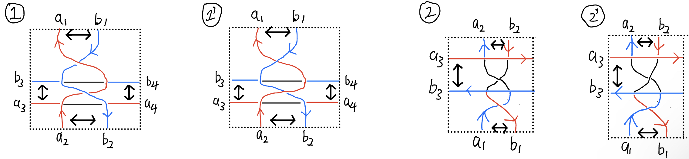
Figure 5.3: $\{a_{i},b_{i}\}$ is a pair of parallel arcs

The black dotted lines indicate that the arcs bounded by it can extend and form arbitrary structure out side it. If two arcs $x\leftrightarrow y$, then I say $\{x,y\}$ (the same as $\{y,x\}$) is a pair of parallel arcs.
Example:

Definition 5.4

: Consider four types of transformation from an oriented open-strand diagram to another in which locally separated arcs intertwine with a pair of parallel arcs to form one of the four structures ①,1'⃝,②,or 2'⃝:

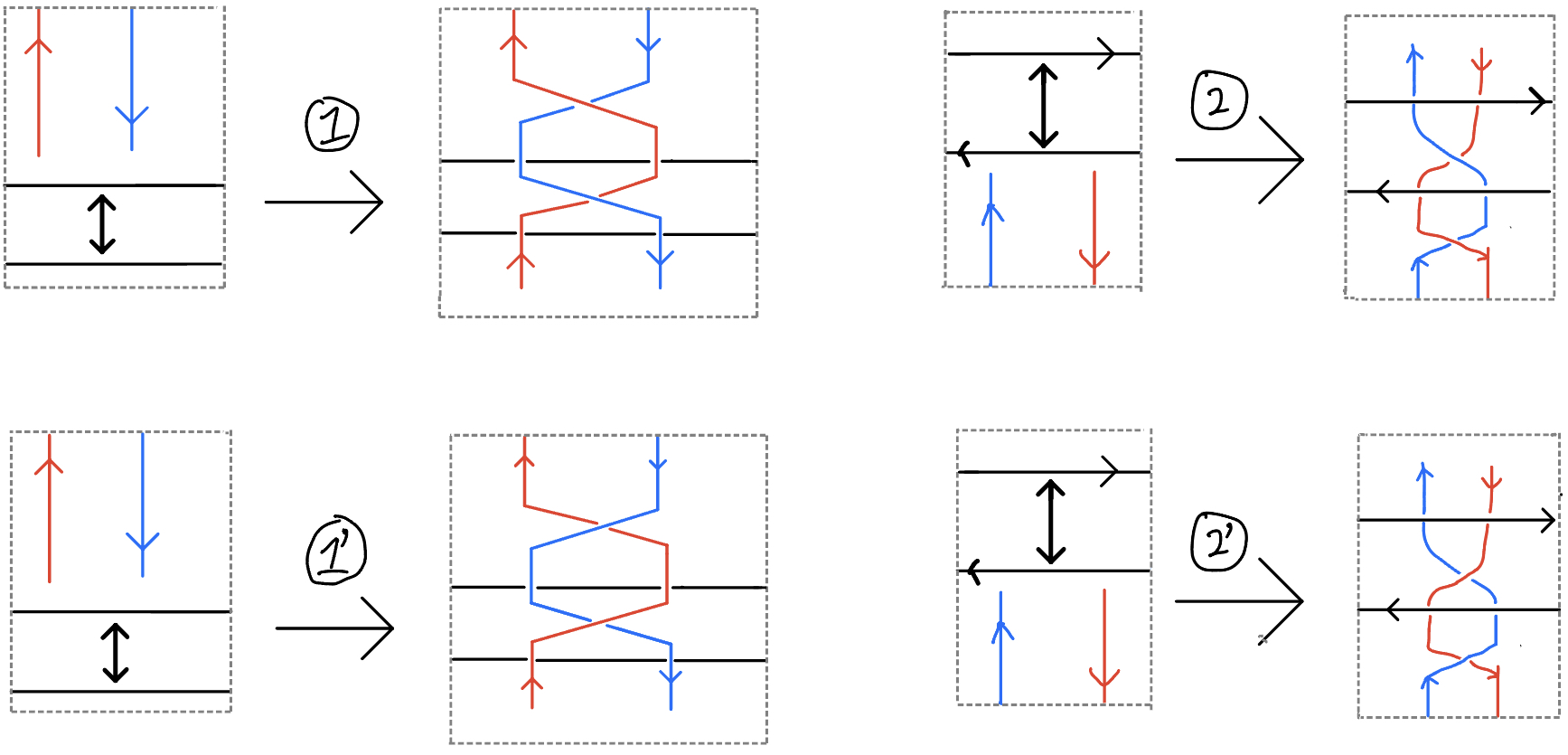
Figure 5.4: move ①,1'⃝,② and 2'⃝

I call these four transformation move ①,1'⃝,② and 2'⃝ respectively. The black,blue,red arrows restrict the orientation of the arcs. The dotted lines indicate that the arcs bounded by it can extend and form arbitrary structure out side it.

Definition 5.5 $L_{m}$ diagram

Consider the set of all oriented open-strand diagrams that can be formed by starting with two separated oppositely oriented line segments going a series of move(s) ①, 1'⃝, ② or 2,⃝.
Let $L_{m}$ denote this type of open-strands diagram. Figure 5.5 gives an example. The following content would focus on the property solely of this type of strand diagrams.

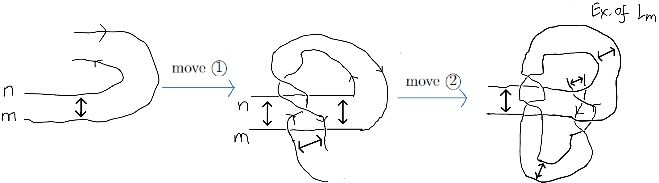
Figure 5.5: example of an type $L_{m}$ diagram

Definition 5.6 path direction for an arc

: Let $L$ be an open-strand diagram. Let $x\in S_{L}$. Fix $a_{0},b_{0}\in E$ such that $a_{0}\nsim_{p}b_{0}$. Then either $x\in P_{a_{0}}$ or $x\in P_{a_{0}}$ by discussion in definition 5.2.2, which show that $\sim_{p}$ is an equivalence relation with 2 equivalence classes. Assume $x\in P_{a_{0}}$. Once we fix $a_{0},b_{0}$ to be the path generator, we can define the path direction for $x$ by the following: Let $x=a_{i}\in P_{a_{0}}=\{a_{0}\to...\to a_{i-1}\to a_{i}\to a_{i+1}\to...\to a_{k}\}$. Then the path direction of $x$ goes from the end of $x$ that connects to $a_{i-1}$ to the other end that connects to $a_{i+1}$, denoted as $e_{a_{i-1}}\to e_{a_{i-1}}$. The only case when this is not defined is when $i=0$ or $i=k$, which means $a_{i}$ is an out-exposed arc. In this case we define $e_{a_{-1}}$ and $e_{a_{k+1}}$ to be the free end of $a_{0},a_{k}$, respectively.
Figure 5.2 shown an example, where the blue and red arrow on the arcs denote the path direction for each arcs.

Properties of $L_{m}$ diagram 5.7

Let $L$ be a type $L_{m}$ diagram with arc set $S_{L}$ and sets of out-exposed arcs $E\subseteq S_{L}$. Then the following properties are proposed:

1. Chose $a_{0},b_{0}\in E$ such that $b_{0}\notin P_{a_{0}}$. Then $\forall x\in S_{L}$, either $x\in P_{a_{0}}$ or $x\in+_{b_{0}}$. This is a direct consequence from discussion in definition 5.2.2, which show that $\sim_{p}$ is an equivalence relation with 2 equivalence classes. Let $P_{a_{0}}=\{a_{0}\to a_{1}\to...\to a_{k}\},P_{b_{0}}=\{b_{0}\to b_{1}\to...\to b_{j}\}$. Then
2.$k=j$ (or $|P_{a_{0}}|=|P_{b_{0}}|$) 3.$\{a_{0},a_{k})\},~{}\{b_{0},b_{k}\}$ are both parallel pair of arcs(definition 5.3).
If $\{x,y\}$ is an unordered pair of parallel arcs, then
4.$x\nsim_{p}y$. Property 4 and 1 implies that either $x\in P_{a_{0}},y\in P_{b_{0}}$ or $x\in P_{b_{0}},y\in P_{a_{0}}$.
5.$\{x,y\}=\{a_{i},b_{i}\}$ for some $i\in\{0,1,...k\}$.
6. In a local space where $x$ and $y$ are geometrically parallel, their path directions are the same, i.e, when represented by arrows projected on the arc in the diagram, they point to the same direction.
(Definition 5.7)let $P^{\prime}_{a_{0}}=\{a_{0}\to a^{\prime}_{1}\to...\to a^{\prime}_{n}\to a_{k}\}$ and $P^{\prime}_{b_{0}}=\{b_{0}\to b^{\prime}_{1}\to...\to b^{\prime}_{m}\to b_{k}\}$ be the ordered subset of $P_{a_{0}}$ and $P_{b_{0}}$ that consisted of only parallel pairs of arcs. Namely, $x\in P^{\prime}_{a_{0}}$ if and only if $x\in P_{a_{0}}$ and $\{x,y\}$ is a pair of parallel arcs for some arc $y$. Property 4 imply that $n=m$. Then
7.For $0\leq i\leq n$, $(a^{\prime}_{i},b^{\prime}_{i})$ and $(a^{\prime}_{i+1},b^{\prime}_{i+1})$ are either horizontally or vertically connected by one of structure ①,1'⃝,②,or 2'⃝. Namely, they are the parallel arcs from one structure in same direction (see figure 5.6). We denote this by $(a^{\prime}_{i},b^{\prime}_{i})\sim_{c}(a^{\prime}_{i+1},b^{\prime}_{i+1})$, which is the same as $(a^{\prime}_{i+1},b^{\prime}_{i+1})\sim_{c}(a^{\prime}_{i},b^{\prime}_{i})$.
8. If the two out-exposed pair of segments are glued together in the diagram for $L$, that is, connecting $a_{0},b_{0}$ together and also connecting $a_{k},b_{k}$ together, then the diagram form a knot that is equivalent to an unknot.
Remark: I will call them proposition 1$\sim$8 in this section(5.7) but property 1$\sim$8 after this section.

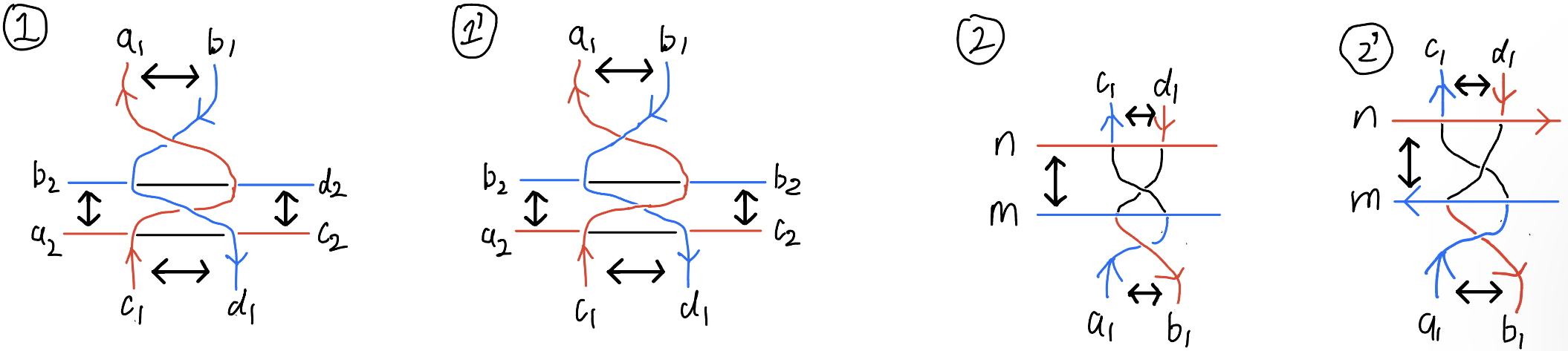
Figure 5.6: illustration for proposition 7. $(a_{k},b_{k})\sim_{c}(c_{k},d_{k})~{}\forall k\in\{1,2\}$

Proof by induction:

base case of induction

The based case is when $L_{1}$ is form by two separated line going through one of move ①,1'⃝,②,or ② for only one time. For both the base case and inductive step, I would only present the proof for the cases for moves ① and ② here, shown in figure 5.7, and the other two moves are very similar and can be checked by the same way easily.

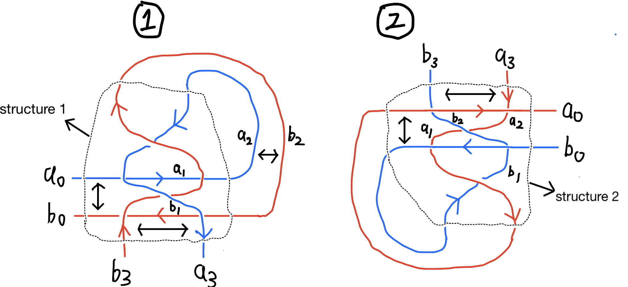
Figure 5.7: $L_{1}$ for move ① and ②

By figure 5.7, For ①, the strand has four out-exposed arcs $a_{0},b_{0},a_{3},b_{3}$ and three pairs of parallel $\{a_{0},b_{0}\},\{a_{2},b_{2}\},\{a_{3},b_{3}\}$. Therefore $P^{\prime}_{a_{0}}=\{a_{0}\to a_{2}\to a_{3}\}$. $P^{\prime}_{b_{0}}=\{b_{0}\to b_{2}\to b_{3}\}$. By this, properties $1\sim 6$ can be easily observed. By the figure, $(a_{0},b_{0})$ and $(a_{2},b_{0})$ are the horizontal parallel pair that are connected by structure ①, whereas $(a_{2},b_{2})$ and $(a_{3},b_{3})$ are vertically connected by the same structure, so property 7 is also satisfied.
For ②, the strand has four out-exposed arcs $a_{0},b_{0},a_{3},b_{3}$ and two pairs of parallel arcs $\{a_{0},b_{0}\}$ and $\{a_{3},b_{3}\}$. Therefore $P^{\prime}_{a_{0}}=\{a_{0}\to a_{3}\},~{}P^{\prime}_{b_{0}}=\{b_{0}\to b_{3}\}$. By this, properties $1\sim 6$ can be easily observed. For ②, $(a_{0},b_{0})$ and $(a_{3},b_{3})$ are vertically connected by a structure ②, so property 7 is satified. Property 8 for both ① and ② is obvious to see.

Inductive step

Suppose $L_{0}$ is a strand diagram that satisfy all 7 propositions, with $P_{a_{0}}=\{a_{0}\to a_{1}\to...\to a_{k}\}$ and $P_{b_{0}}=\{b_{0}\to b_{1}\to...\to b_{k}\}$. In order for it to go though one of the 4 types of move, either $(a_{0},b_{0})$ or $(a_{k},b_{k})$ must be the vertical pair of arcs involved in the move(see figure 5.4) because one end of the vertical pair at the start of all moves must be out-exposed, as shown in figure 5.3. With out lost of generality, we can assume that $(a_{k},b_{k})$ is the one involved in the move. Also, there must exist a pair of parallel arcs at the exterior of the knotted part (bounded by dotted curve in figure 5.8 and 5.9) between the starting and ending pair, which serve as the horizontal pair in the move that the vertical pair of arcs pass above or below in the moves. By proposition 5, there exist $i\in\{0,1,...k\}$ such that $(a_{i},b_{i})$ is the parallel arcs. With out lost of generality, we can assume that the arc on the top to be $a_{0}$. Thus, $L_{0}$ and the the possible results after it goes through move ① or ② to form $L_{0+1}$ and $L_{0+2}$ respectively can be presented as one of the two cases shown below:

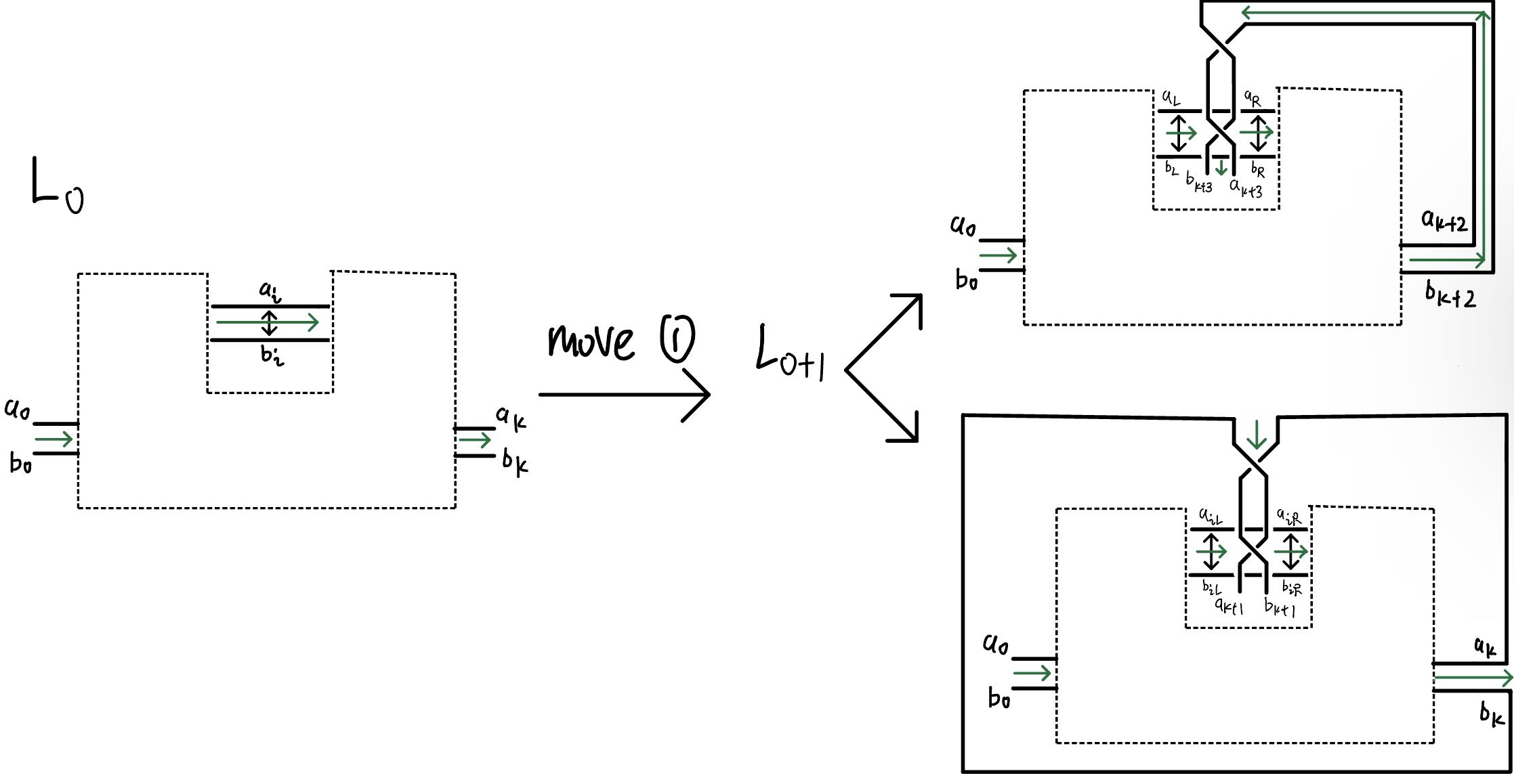
Figure 5.8: $L_{0}$ going through move ①

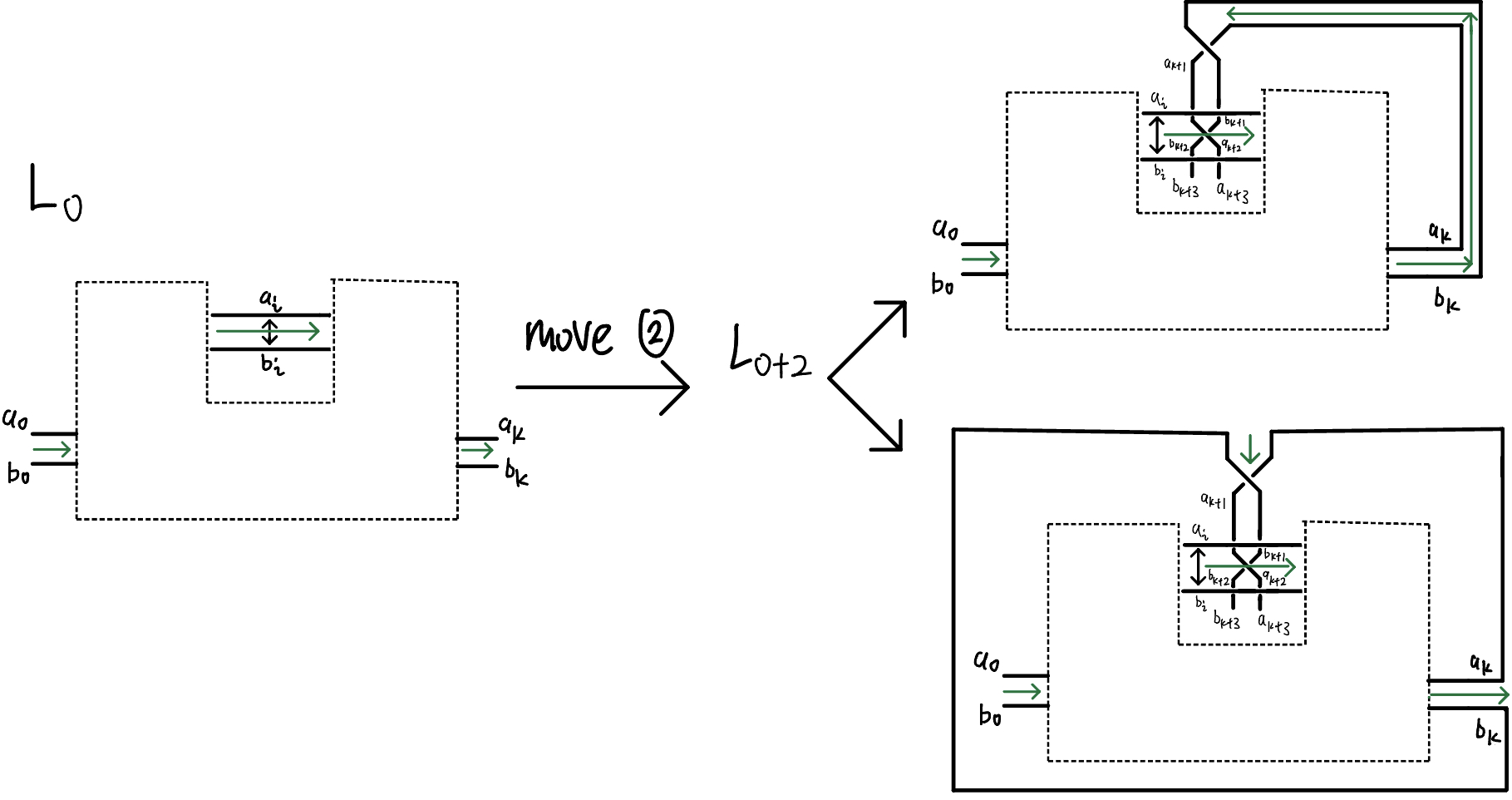
Figure 5.9: $L_{0}$ going through move ②

To show the 8 propositions:

By proposition 6, the path direction for $a_{i}$ and $b_{i}$ should be the same. With out the lost of generality, we can assume that the path for both goes from left to right, which imply that in $L_{0}$, the two arcs connected to the the left end of $a_{i},b_{i}$ is $a_{i-1}$ and $b_{i-1}$, respectively. Then in $L_{0+1}$, $L=i,m=i+1,R=i+2$, so $(a_{k},b_{k})$ in $L_{0}$ is replaced by $(a_{k+2},b_{k+2})$.
Then for $L_{0+1}$, $P_{a_{0}}=\{a_{0}\to...\to a_{L}\to a_{m}\to a_{R}\to...\to a_{k+2}\to a_{k+3}\}$,
$P_{b_{0}}=\{b_{0}\to...\to b_{L}\to b_{m}\to b_{R}\to...\to b_{k+2}\to b_{k+3}\}$.
For $L_{0+2}$, $P_{a_{0}}=\{a_{0}\to...\to a_{k+1}\to a_{k+2}\to a_{k+3}\}$,
$P_{b_{0}}=\{b_{0}\to...\to b_{k=1}\to b_{k+2}\to b_{k+3}\}$. Property 2,3 is therefore satisfied.
In $L_{0+1}$, the new pair of parallel arcs created are $\{a_{L},b_{L}\},\{a_{R},b_{R}\},\{a_{k+1},b_{k+1}\}$ and $\{a_{k+3},b_{k+3}\}$. This satisfy proposition 4. The path direction for $a_{L},b_{l},a_{R},b_{R}$ all goes from left to right, therefore satisfy proposition 6. The path directions for $\{a_{k+1},b_{k+1}\}$ and $\{a_{k+3},b_{k+3}\}$,as shown by the green arrows, also satisfy it. Their index number that we already calculated in $P_{a_{0}}$ and $P_{a_{0}}$ satisfy proposition 5. By inductive assumption on proposition 7, in $L_{0}$, $(a_{i},b_{i})$ is connected with both $(a_{i-1},b_{i-1})$ and $(a_{i+1},b_{i+1})$ by some structure. So in $L_{0+1}$, $(a_{L}(a_{i}),b_{L}(b_{i}))\sim_{c}(a_{i-1},b_{i-1})$, $(a_{R}(a_{i+2}),b_{R}(b_{i+2}))\sim_{c}(a_{i+3},b_{i+3})$ and by the graph $(a_{L},b_{L})\sim_{c}(a_{R},b_{R})$ and $(a_{k+2},b_{k+2})\sim_{c}(a_{k+3},b_{k+3})$, which means all new parallel arcs in $L_{0+1}$ satisfy proposition 7. Other possible pair of parallel arcs, which locate inside the area bounded by dotted line, remain unchanged as they are in $L_{0}$, so they also satisfy proposition 4,5,6,7, which are therefore generally true in $L_{0+1}$.
In $L_{0+2}$, the only new pair of parallel pair created is $\{a_{k+3},b_{k+3}\}$, which satisfy proposition 4. The graphs and the index number calculated show $\{a_{k+3},b_{k+3}\}$ satisfies proposition 5. The graph also show that $(a_{k+3},b_{k+3})\sim_{c}(a_{k+1},b_{k+1})$, which satisfy proposition 7. So both $L_{0+1}$ and $L_{0+2}$ satisfy property 2$\sim$ 7.
To show proposition 8, notice that the knots form by gluing the starting and ending pair for both $L_{0+1}$ and $L_{0+2}$ (denoted as $K_{L_{0+1}}$ and $K_{L_{0+2}}$) can be deform back to the knot form by gluing the starting and ending pair of $L_{0}$ (denoted as $K_{L_{0}}$) by applying only Reidemeister moves $II$ and $III$, as shown figure below.

This show $K_{L_{0+1}}$ and $K_{L_{0+2}}$ are both equivalent to $K_{L_{0}}$. Since by the inductive hypothesis, $K_{L_{0}}$ is equivalent to unknot, so do $K_{L_{0+1}}$ and $K_{L_{0+2}}$, which shows proposition 8.

Definition 5.8 ordered pair of parallel arcs

By property 1 and 3 in section 5.7, there are two out-exposed pair of parallel arcs in any $L$ be a type $L_{m}$ strand diagram, so we can freely chose one of the two pair to be the starting pair and the other to be the end pair of $L$, denoted as $\{a_{0},b_{0}\}$ and $\{a_{e},b_{e}\}$, respectively such that $a_{0}\sim_{p}a_{e},~{}b_{0}\sim_{p}b_{e}$. Once we fix the order between $a_{0}$ and $b_{0}$ to define the ordered starting pair of $L$, say $(a_{0},b_{0})$, we define the ordered ending pair of arcs to be $\{a_{e},b_{e}\}$. Similarly, for any parallel pair of arcs $\{x,y\}$, by property 4, we can define the corresponded ordered parallel pair of arcs be $(x,y)$ if $x\sim_{p}a_{0}$ and $(y,x)$ if $x\sim_{P}b_{0}$.
By this definition, if $(x,y),(a,b)$ are two arbitrary ordered pair of parallel arcs, then $x\sim_{p}a,~{}y\sim_{p}b$.

Definition 5.9 path direction for $L_{m}$ diagram

By property 6 in section 5.7, if $(x,y)$ is an ordered pair of parallel arcs, in any local space where $x,y$ are geometrically parallel, the path direction for $x$ and for $y$ is the same. So once we fix the starting pair of arcs as well as fixing the generator for all two paths for $L$. we can define the path direction for the pair $(x,y)$ in that local space to be the path direction for $x$, represented by green arrow that travel between $x$ and $y$ shown in figure below:

Definition 5.10 directional version of moves ①, 1'⃝, ② and 2'⃝

By definition 5.9, we can restrict the path direction for the two pairs of parallel arcs involved in the moves ①, 1'⃝, ② shown in figure 5.4 to define 8 directional moves 1.1,1.2,$1.1^{\prime}$,$1.2^{\prime}$,2.1,2.2,$2.1^{\prime}$,$2.2^{\prime}$ in the graph below:

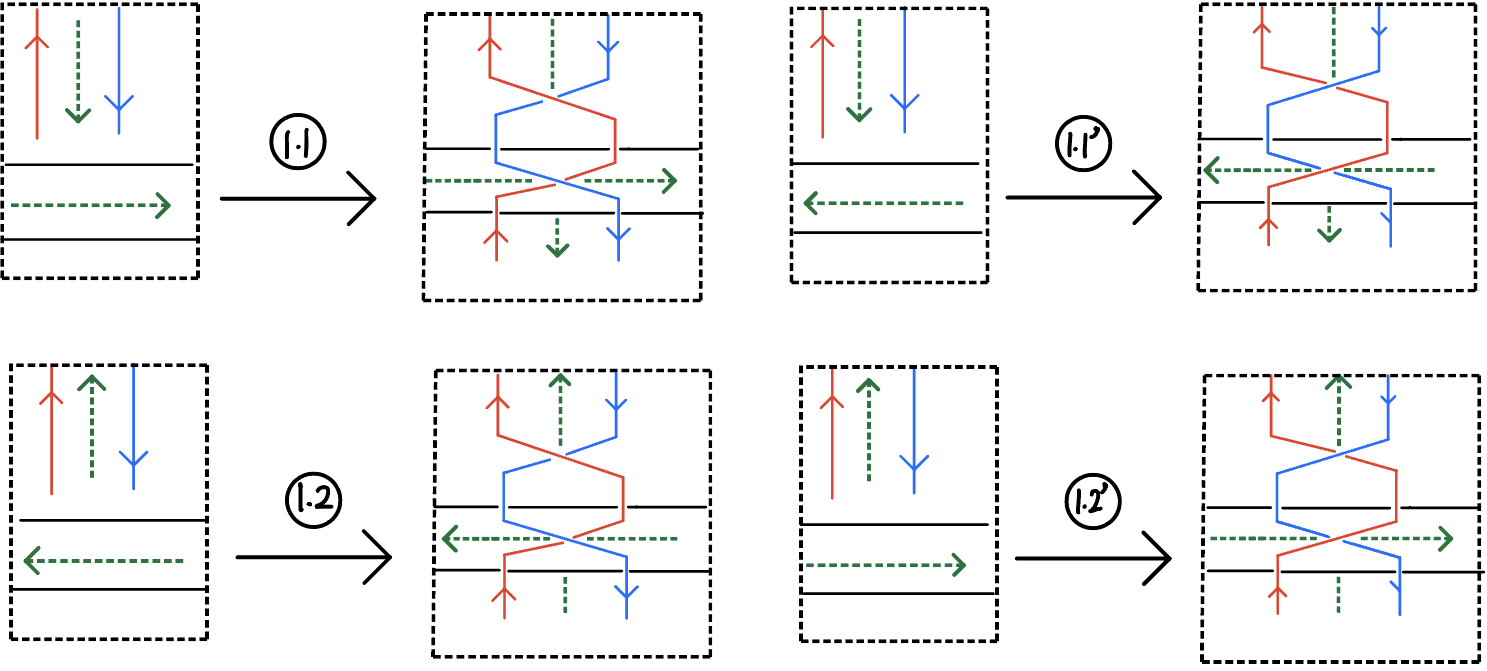
Figure 5.10: directional moves 1.1,1.2 form structure ①, moves $1.1^{\prime}$,$1.2^{\prime}$ form structure ②.

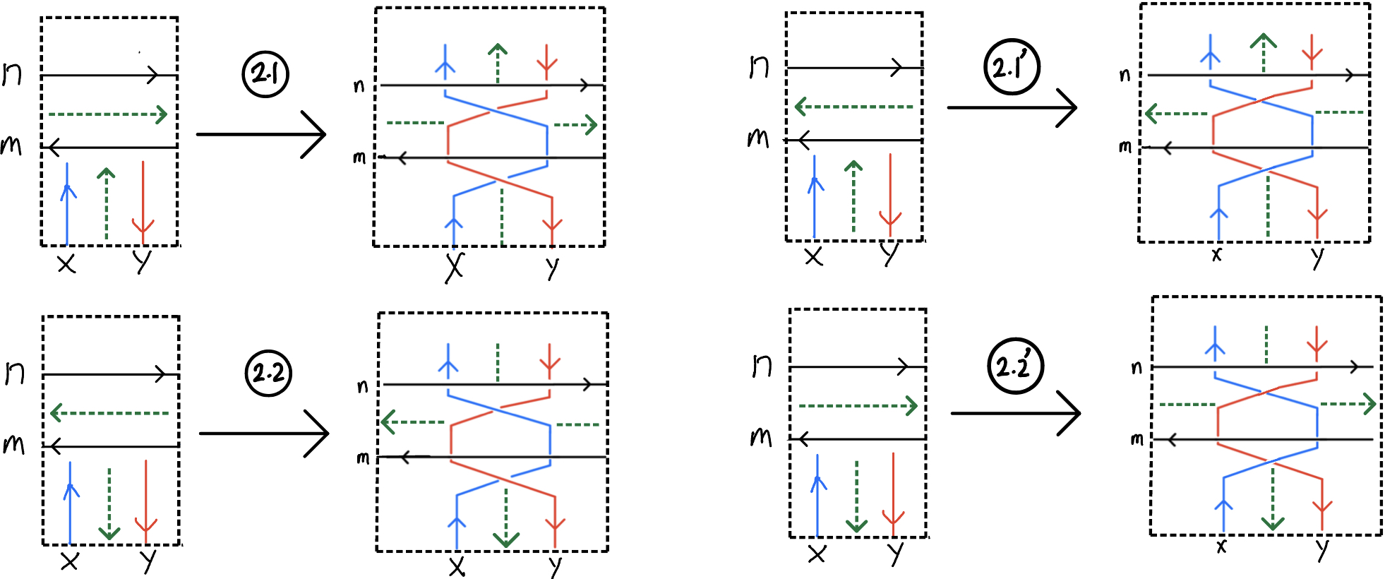
Figure 5.11: directional moves 2.1,2.2 form structure ②, moves $2.1^{\prime}$,$2.2^{\prime}$ form structure 2'⃝.

Definition 5.11 type $L_{om}$ diagram

We can modified definition 5.5 by restricting the 4 moved to be all directional moves to define $L_{om}$ diagram to be the type of open-strands diagram that can be formed by applying only directional move 1.1,1.2,$1.1^{\prime}$,$1.2^{\prime}$,2.1,2.2,$2.1^{\prime}$,$2.2^{\prime}$ on two separated oppositely oriented line segments.
Figure 5.13 show that $T$ in figure 3.2 is a type $L_{om}$ diagram. The figure below give a non-tangle example of a $L_{om}$ diagram, whose transformation process is shown below it, by setting the path direction to be from left to right in the initial state (two separated line).

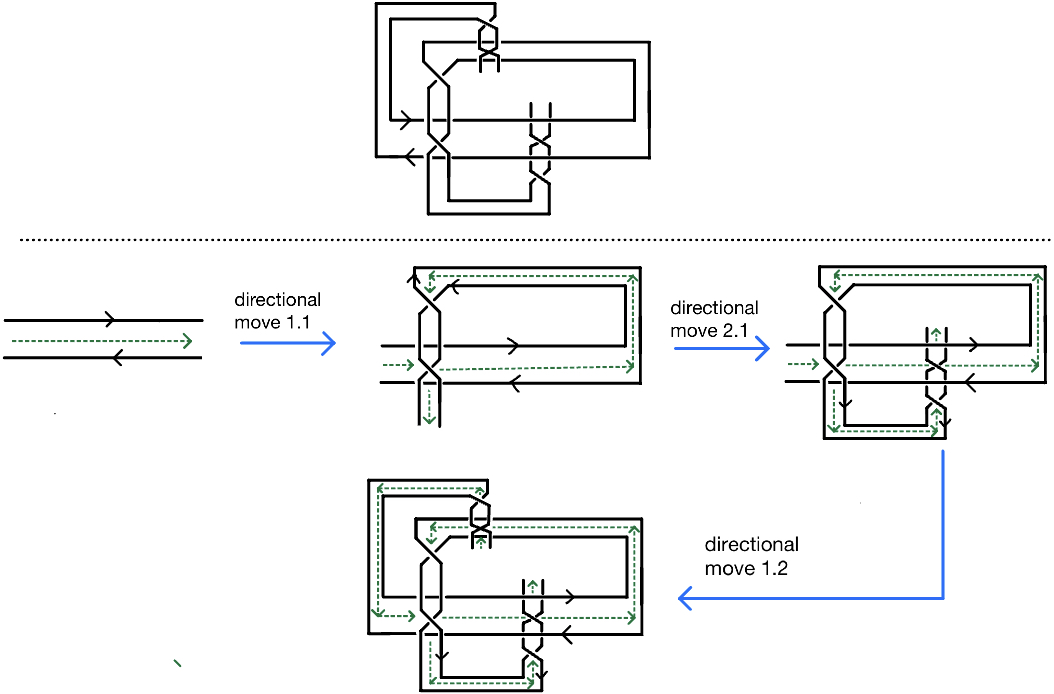
Figure 5.12:

With these properties, the following theorem can be proposed and proved:

Theorem 5.1

: Let $Q(*)$ be a medial quandle (definition 2.6). Let $L$ be an arbitrary $L_{om}$ diagram with ordered starting and end pair or arcs be $\{a_{0},b_{0}\}$ and $\{a_{e},b_{e}\}$, respectively. Then the system of equations given by all crossing relations in $L$ under the operation in $Q(*)$ requires the solution to satisfy $a_{0}=a_{e},b_{0}=b_{e}$. In another word, if we consider $Hom(L,Q(*))$, the coloring space on $L$ by $Q(*)$, $\forall f\in Hom(L,Q(*))$, it must be true that $f(a_{0})=f(a_{e}),f(b_{0})=f(b_{e})$. This result also hold for any open-strand diagram that can be transform by some type $L_{om}$ diagram by only applying Reidemeister moves because the quandle coloring is an invariant under Reidemeister moves. $L_{p}$ is one such example as shown in figure 5.13, so lemma 1 in section 4.2 is a specific case of Theorem 5.1.

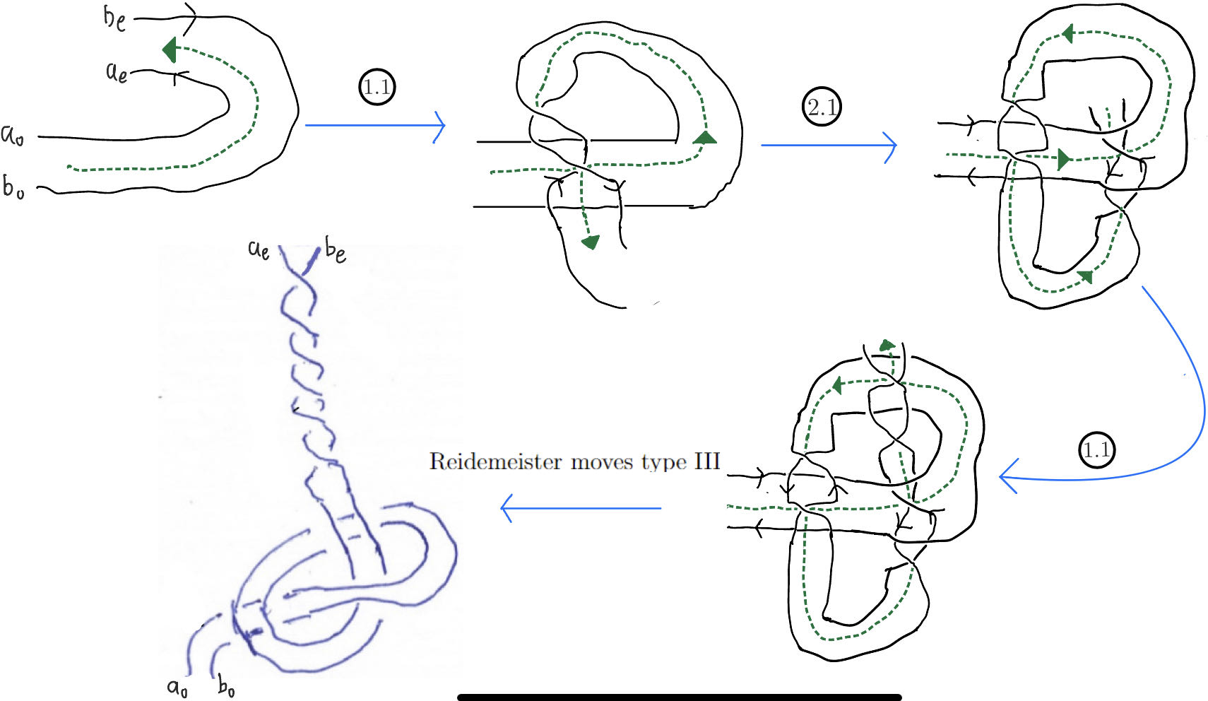
Figure 5.13: the tangle $T$(or $L_{p}$) is an example type $L_{m}$ open-strand diagram. Theorem 5.1 implies that any coloring from a medial quandle result in $a_{0}=a_{e},b_{0}=b_{e}$

6 Proof of theorem 5.1

6.1 properties of medial quandle

Recall the following properties proved at the start of section 4. Let $Q(*)$ be a medial quandle. Then
1.$[(a*x)*^{-1}y]*z=[(a*z)*^{-1}y]*x,~{}\forall a,x,y,z\in Q$.
2. $[(a*^{-1}x)*y]*^{-1}z=[(a*^{-1}z)*y]*^{-1}x$.

definition 6.1

For any $x,y\in Q$, define $f_{xy}:Q\to Q$ by $f_{xy}(q)=(q*^{-1}x)*y$.
Let $f_{x_{2}y_{2}}\circ f_{x_{1}y_{1}}(q):=f_{x_{2}y_{2}}(f_{x_{1}y_{1}}(q))$ denote the composition of two such function. Then $\forall x,y,a,b,q\in Q$,

4. $f_{xy}\circ f_{ab}=f_{ab}\circ f_{xy}$.
5. $f_{1}\circ f_{2}\circ...\circ f_{k}=f_{1^{\prime}}\circ f_{2^{\prime}}\circ...\circ f_{k^{\prime}}$, where $\{i\}\to\{i^{\prime}\}$ is a permutation, and $f_{i}=f_{x_{i}y_{i}}$ for some $x_{i},y_{i}\in Q$.
6. $f_{xy}(a*b)=f_{xy}(a)*f_{xy}(b)$ and $f_{xy}(a*^{-1}b)=f_{xy}(a)*^{-1}f_{xy}(b)$.
7.Let $f_{c}=f_{x_{1}y_{1}}\circ...\circ f_{x_{k}y_{k}}$ for some $x_{i},y_{i}\in Q(*)$. Then $f_{c}(a*b)=f_{c}(a)*f_{c}(b)$ and $f_{c}(a*^{-1}b)=f_{c}(a)*^{-1}f_{c}(b),~{}\forall a,b\in Q(*)$. Proof:
The properties in section 2.6 are enough to show that $Q$ is also a medial quandle under the inverse operation $*^{-1}$. Property 6 show each $f_{x_{i}y_{i}}$ is quandle endomorphism on both $Q(*)$ and $Q(*^{-1})$. So $f_{c}$ is the composition of some homomorphisms, so $f_{c}$ has to be a homomorphism on $Q(*)$ and $Q(*^{-1})$, which means $f_{c}(a*b)=f_{c}(a)*f_{c}(b)$ and $f_{c}(a*^{-1}b)=f_{c}(a)*^{-1}f_{c}(b)$.

Remark:In some computation process in section 6, $=_{(i)}$ or $=_{k}$ means that the right side of the equation are derived by applying property $(i)$ in section 2.6 or property $k$ presented in this section.

6.2 medial quandle’s coloring on four structures

Let first analysis the coloring on structure ①, 1'⃝, ② and 2'⃝ (definition 5.2).

In all 4 structure by labeling 4 of the arcs exposed outside with $x,y,n,m$ representing some element in $Q(*)$, the other 4 out-exposed aces labeled by $x^{\prime},y^{\prime},n^{\prime},m^{\prime}$ can be expressed by a string of quandle operations between $x,y,n,m$. By using the properties of distributive quandle given in section 2.6, these expressions can be further simplified to the form of some functions $f_{pq},~{}p,q\in\{x,y,n,m\}$ defined in definition 4.1 acting on one of $x,y,n,m$ The result is shown in the figure below and the calculation process is shown below.

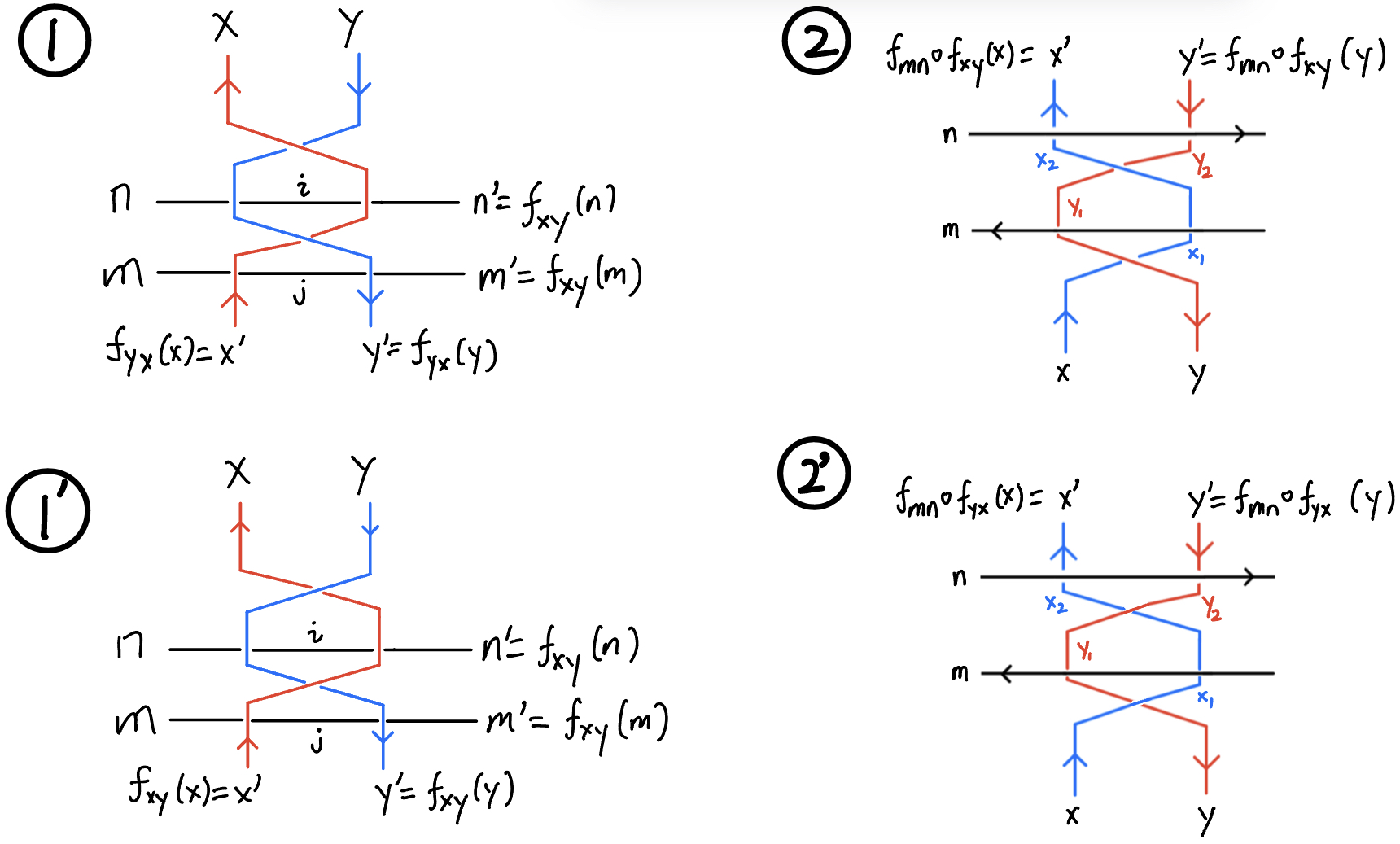
Figure 6.1: medial quandle’s coloring on four quandle

For structure ①:
$y^{\prime}=y*x=(y*^{-1}y)*x=f_{yx}(y)$
$x^{\prime}=x*^{-1}y^{\prime}=x*^{-1}(y*x)=(x*^{-1}y)*(x*^{-1}x)=(x*^{-1}y)*x=f_{yx}(x)$
$n^{\prime}=i*^{-1}x=(n*y^{\prime})*^{-1}x=[n*(y*x)]*^{-1}x=[(n*^{-1}x)*[(y*x)*^{-1}x]]=(n*^{-1}x)*y=f_{xy}(n)$.
$m^{\prime}=j*y^{\prime}=(m*^{-1}x^{\prime})*(y^{\prime})=[m*^{-1}[(x*^{-1}y)*x]]*(y^{\prime})=(m*y^{\prime})*^{-1}[[(x*^{-1}y)*x]*y^{\prime}]=(m*y^{\prime})*^{-1}[[(x*^{-1}y)*x]*(y*x)]=[m*(y*x)]*^{-1}x=(m*^{-1}x)*[(y*x)*^{-1}x]=(m*^{-1}x)*y=f_{xy}(m)$.
For structure 1'⃝:
$x^{\prime}=x*y=(x*^{-1}x)*y=f_{xy}(x)$
$y^{\prime}=y*^{-1}x^{\prime}=y*^{-1}(x*y)=(y*^{-1}x)*y=f_{xy}(y)$
$n^{\prime}=i*^{-1}x^{\prime}=(n*y)*^{-1}(x^{\prime})=(n*y)*^{-1}(x*y)=(n*^{-1}x)*y=f_{xy}(n)$
$m^{\prime}=j*y^{\prime}=(m*^{-1}x^{\prime})*y^{\prime}=[m*^{-1}(x*y)]*y^{\prime}=[(m*^{-1}x)*(m*^{-1}y)]*[(y*^{-1}x)*y]=$
$[(m*^{-1}x)*(y*^{-1}x)]*[(m*^{-1}y)*y]=[(m*y)*^{-1}x]*m=_{1}[(m*m)*^{-1}x]*y=(m*^{-1}x)*y=f_{xy}(m)$.
For structure ②:$x_{1}=x*y~{}~{}x_{2}=x_{1}*^{-1}m~{}~{}y_{1}=y*^{-1}m~{}~{}y_{2}=y_{1}*^{-1}x_{2}$, so
$x^{\prime}=x_{2}*n=(x_{1}*^{-1}m)*n=[(x*y)*^{-1}m]*n=[[(x*^{-1}x)*y]*^{-1}m]*n=f_{mn}\circ f_{xy}(x)$
$y^{\prime}=y_{2}*n=(y_{1}*^{-1}x_{2})*n=[(y*^{-1}m)*^{-1}(x_{1}*^{-1}m)]*n=[(y*^{-1}x_{1})*^{-1}m]*n=[[y*^{-1}(x*y)]*^{-1}m]*n=[[(y*^{-1}x)*y]*^{-1}m]*n=f_{mn}\circ f_{xy}(y)$
For structure 2'⃝: We can skip the calculation proccess by comparing it with structure ②. The crossing relations given by structure ② are $\{x*y=x_{1},~{}y*^{-1}m=y_{1},~{}x_{1}*^{-1}m=x_{2},~{}y_{2}*x_{2}=y_{1},~{}x_{2}*n=x^{\prime},~{}y_{2}*n=y^{\prime}\}$. Switching every $x-$family with the correspond $y-$ family in this set give exactly the set of crossing relations given by structure 2'⃝. Do the calculation result for structure 2'⃝ can be derived by switching all $x(x^{\prime})$ with $y(y^{\prime})$ in the result for structure ①, namely,
$y^{\prime}=[[(y*^{-1}y)*x]*^{-1}m]*n=f_{mn}\circ f_{yx}(y)$
$x^{\prime}=[[(x*^{-1}y)*x]*^{-1}m]*n=f_{mn}\circ f_{xy}(x)$.

6.3 coloring on type $L_{om}$ diagram

Let $L$ be an arbitrary type $L_{om}$ strand diagram (definition 3.10). By property 1 in section 5.7, we can fix the ordered starting and ending pair of arcs of $L$ to be $(a_{0},b_{0})$ and $(a_{e},b_{e})$ respectively, and let $p^{\prime}_{a_{0}}=\{a_{0}\to a_{1}\to...a_{k}\to a_{e}\},p^{\prime}_{b_{0}}=\{b_{0}\to b_{1}\to...b_{k}\to b_{e}\}$ be the path of $L_{om}$ that consisted of only parallel arcs where $k$ is a positive integer. We want to show that any coloring from a medial quandle $Q(*)$ requires $a_{0}=a_{e},b_{0}=b_{e},$ or $(a_{0},b_{0})=(a_{e},b_{e})$ (theorem 5.1).

proposition 3.3.1

$\forall p,j\in\{0,1,...k,e\}$, there exist $x_{i},y_{i}\in Q(*)$ such that $(a_{j},b_{j})=f_{x_{1}y_{1}}\circ...\circ f_{x_{r}y_{r}}((a_{p},b_{p}))$. Here we use the denotation $f_{xy}((a,b)):=(f_{xy}(a),f_{xy}(b))$, mapping from pair of arc to another pair of arc.

Proof: Assume that $j>p$. For all $i\in\{0,1,...k\}$, by property 7 in section 5.7 and checking each structure in figure 6.1, $(a_{i+1},b_{i+1})=(f_{c}(a_{i}),f_{c}(b_{i}))$ where we let $f_{c}$ denote one single or the composition of some $f_{p_{i}q_{i}}$ functions for some $p_{i},q_{i}\in Q(*)$. So $a_{j}=f_{c_{1}}(a_{j-1}),~{}a_{j-1}=f_{c_{2}}(a_{j-2}),...,a_{(}p+1)=f_{c_{j-p}}(a_{p})$, which is the same for b. This imply $a_{j}=f_{c_{1}}\circ...\circ f_{c_{j-p}}(a_{p}),~{}b_{j}=f_{c_{1}}\circ...\circ f_{c_{j-p}}(b_{p})$, which complete the proof of proposition 3.1.1 if $j>p$ because each $f_{c_{i}}$ is the composition of some $f_{xy}$ function. However, the relation between $p,j$ does not matters because if $p>j$, we proved that $(a_{p},b_{p})=f_{c}((a_{j},b_{j}))$. Since for any $x,y\in Q(*),~{}f_{xy}$ has inverse function $f_{yx}$, we have $(a_{p},b_{p})={f_{c}}^{-1}((a_{j},b_{j}))$ where ${f_{c}}^{-1}$ is also the type of composite function required in the proposition. If $p=j$, then $(a_{j},b_{j})=(a_{p}=f_{a_{p}a_{p}}(a_{p}),b_{p}=f_{a_{p}a_{p}}(b_{p}))$, so $(a_{j},b_{j})=f_{a_{p}a_{p}}((a_{j},b_{j}))$.

proposition 3.3.2

In a type $L_{om}$ diagram, if two ordered pair of parallel arcs $(a,b),(a^{\prime}b^{\prime})$ is (vertically) connected by ② or 2'⃝, then $a=a^{\prime},b=b^{\prime}$. Referring on figure 6.1, this is stating that for both ② and 2'⃝ $x^{\prime}=x,y^{\prime}=y$ no matter what other part of the diagram looks like.

Proof: Referring to the labels in figure 5.11,by property 4 in section 5.7, either
$x\sim_{p}n,y\sim_{p}m~{}$$(1)$ or $x\sim_{p}m,y\sim_{p}n$$(2)$. We first show that structure ② must satisfy $(1)$ and structure 2'⃝ must satisfy $(2)$.To prove this claim, For structure ②, suppose for the sake of contradiction that $(2)$ is true, which means $m\sim_{p}x$. For both 2.1 and 2.2 in figure 5.11, the path directions (represented by green arrows) for the pairs imply it must be the right end of $m$ that connects to $x$ through a path. This means there exist a series of distinct arcs $x_{1},x_{2},..x_{k}$ such that $m\sim x_{1}\sim x_{2}\sim...\sim x_{k}\sim x$, shown by the graph below:

However, this case is impossible to exist because the orientation of arcs $x$ and $x_{k}$(represented by blue and black arrows) contradicts. By applying the same argument on $2.1^{\prime},~{}2.2^{\prime}$ in figure 5.11 which represent possible path directions for structure 2'⃝ in a type $L_{om}$ diagram, it can be shown that the opposite condition, $(1)$, is impossible to be satisfied by structure 2'⃝.
Now referring to figure 6.1, for ②, $(1)$ is true, so $(n,m),(x,y)$ are ordered pair of parallel arcs. So proposition 3.3.1 can be apply to show that $x=f_{v_{1}w_{1}}\circ f_{v_{2}w_{2}}\circ...\circ f_{v_{p}w_{p}}(x),y=f_{v_{1}w_{1}}\circ f_{v_{2}w_{2}}\circ...\circ f_{v_{p}w_{p}}(y)$ for some $v_{1},w_{i}\in Q(*)$. Let $f_{c}:=f_{v_{1}w_{1}}\circ...\circ f_{v_{p}w_{p}}$. Then the calculation in figure 6.1 gives
$x^{\prime}=f_{mn}f_{xy}(x)=f_{mn}([x*y])=f_{mn}([f_{c}(n)*f_{c}(m)])=_{7}f_{mn}([f_{c}(n*m)])=_{5}f_{c}(f_{mn}(n*m))=f_{c}([(n*m)*^{-1}m]*n)=f_{c}(n)=x$ $(I)$
$y^{\prime}=f_{mn}f_{xy}(y)=f_{mn}([(y*^{-1}x]*y)=f_{mn}([(f_{c}(m)*^{-1}f_{c}(n))*f_{c}(m)])=_{7}\\ f_{mn}(f_{c}([(m*^{-1}n)*m])=_{5}f_{c}(f_{mn}([(m*^{-1}n)*m]))=f_{c}([[(m*^{-1}n)*m]*^{-1}m]*n)=f_{c}([(m*^{-1}n)*n])=f_{c}(m)=y$ $(II)$
For structure 2'⃝,$(2)$ is true, so similarly we can conclude that $x=f_{c}(m),y=f_{c}(n)$, where $f_{c}$ is the composition of some $f_{x_{1}y_{1}}$. Then
$x^{\prime}=f_{mn}\circ f_{yx}(x)=f_{mn}([(x*^{-1}y)*x])=f_{mn}([(f_{c}(m)*^{-1}f_{c}(n))*f_{c}(m)])=_{(II)}=f_{c}(m)=x$
$y^{\prime}=f_{mn}\circ f_{yx}(y)=f_{mn}([y*x])=f_{mn}([f_{c}(n)*f_{c}(m)])=_{(I)}=f_{c}(n)=y$
This complete the proof for proposition 3.3.2.

We now prove theorem 5.1. By property 7 in section 5.7 and computation of each structure in figure 6.1, for all $i\in\{0,1,...k\}$, if $(a_{i},b_{i})$, $(a_{i+1},b_{i+1})$ is connected by structure ① or 1'⃝, then $(a_{i+1},b_{i+1})=f_{xy}((a_{b},b_{i})$, where $\{x,y\}$ is the vertical pair of parallel arcs of that structure (note that $\forall p,q,x,y\in Q(*)$, if $q=f_{xy}(q)$, then $p=f_{yx}(q)$). If $(a_{i},b_{i})$, $(a_{i+1},b_{i+1})$ is connected by structure ② or 2'⃝, then $(a_{i},b_{i})=(a_{i+1},b_{i+1})$ by proposition 6.3.2. Since we can write $(a_{1},b_{1})=f_{0}((a_{0},b_{0})),(a_{2},b_{2})=f_{1}((a_{1},b_{1})),...(a_{e},b_{e})=f_{k}((a_{k},b_{k}))$, where each $f_{i}=f_{x_{i}y_{i}}$ or be the identity function. This means we can write
$(a_{e},b_{e})=f_{k}\circ f_{k-1}\circ...\circ f_{0}((a_{0},b_{0}))$ (1).
After throwing out all identity function, each $f_{i}$ is by definition uniquely corresponded to two pairs of parallel arcs that are either horizontally or vertically connected by a structure ① or 1'⃝ with restriction on their path direction, shown in figure 5.10. By definition, the path direction goes from $(a_{i},b_{i})$ to $(a_{i+1},b_{i+1})$ (from smaller index to bigger index). For all four move 1.1,1.2,$1.1^{\prime}$,$1.2^{\prime}$,by comparing the ending structure in figure 5.10 with the computation for structure ① and 1'⃝ in figure 6.1, we can conclude that if $f_{i}=f_{x_{i}y_{i}}$ is contributed by two pairs of arcs horizontally/vertically connected by the strcuture, then the pairs of arcs vertically/horizontally connected by the structure contribute to a tern $f_{i^{\prime}}=f_{yx}={f_{i}}^{-1}$. This means we can rearrange functions in (1) (property 5 in 6.1 allows this) to
$(a_{e},b_{e})=f_{1}\circ f_{1^{\prime}}\circ f_{2}\circ f_{2^{\prime}}\circ...\circ f_{p}\circ f_{p^{\prime}}((a_{0},b_{0}))$ such that $f_{i^{\prime}}={f_{i}}^{-1},~{}\forall i\in\{1,...,p\}$. This composited function is nothing but composition of $p$ identity function, which means $(a_{e},b_{e})=(a_{0},b_{0})$, which completes the proof for theorem 5.1

7 application of theorem 5.1

Theorem 5.1 can be used to check the coloration of medial quandle to both some knots and links that contains type $L_{om}$ strands as its main body.

7.1 example of application on knot

Proposition 7.1

Any knot in the form shown by figure 7.1, derived by simply intertwine the starting and ending pair of an type $L_{om}$ diagram, can not be differentiated from the unknot by medial quandles.

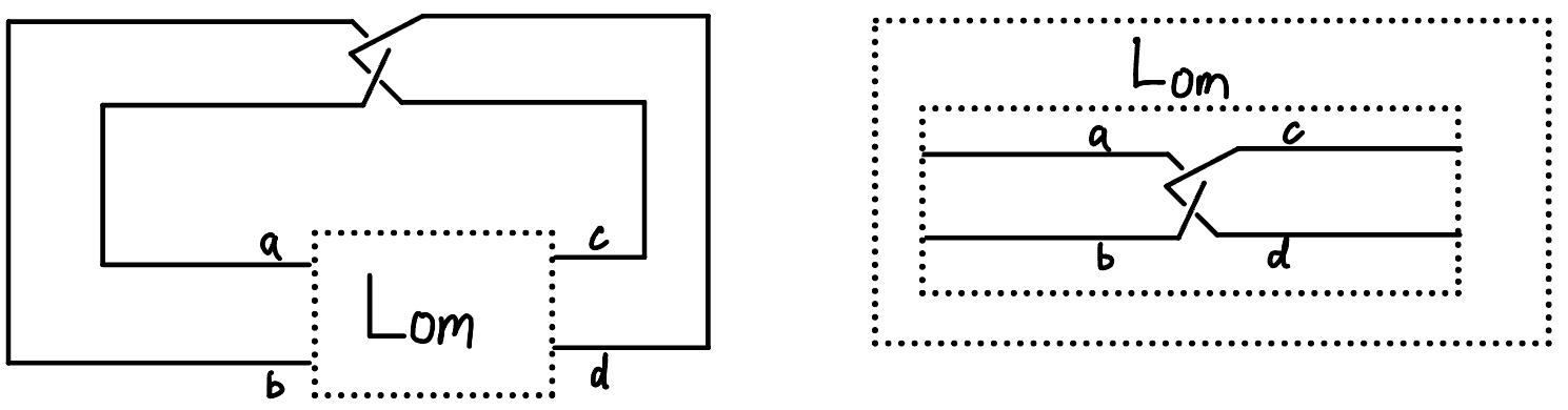
Figure 7.1: $k_{om}$

Proof:

Let’s denote this type of knot by $K_{om}$. By theorem 5.1, either $a=c,b=d$ or $a=d,b=c$. In either case, after setting an orientation for the knot restricted by the condition, one can show that the two crossing between the starting and ending pair requires $a=b=c=d$, particularly, $a=b$ and $a=c$. This imply the system of crossing relation generated by $K_{om}$ contains the system of crossing relations given by the knot form by simply gluing $a,c$ together and $b,d$ together in the $L_{om}$ diagram. By property 8 in section 5.7, the latter degenerate to an unknot. So the coloring space for $K_{om}$ must be a subset of that of an unknot. But the coloring space on an unknot is the smallest possible coloring space containing only trivial coloring, so the coloring space on $K_{om}$ is the same as that on an unknot, as desired.

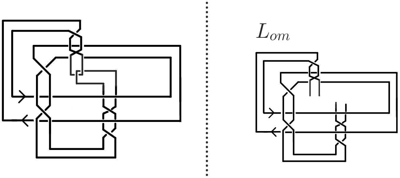
Figure 7.2: An example of the type of knot shown in figure 7.1 (left), which is indistinguishable from the unknot by medial quandle’s coloring. See figure 5.12 for the formation of its correspond $L_{om}$ open-strand diagram(right).

7.2 example of application on links

Proposition 7.2 (application on two-component link)

An medial quandle $Q(*)$ such that the relation $\sim$ on $Q$ defined by $a*b=a\leftrightarrow a\sim b$ is an equivalence relation cannot distinguish between two-component links in the form shown in figure below at the left and the Hopf link.

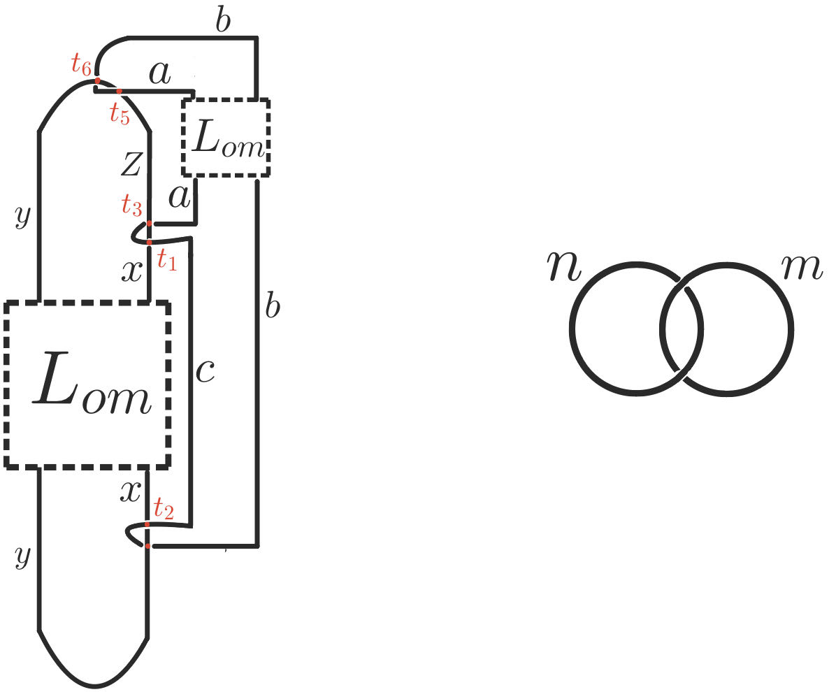
Figure 7.3: a type of two-component links (left) and the Hopf link (right) that is indistinguishable from each other by $Q(*)$

Proof for proposition 7.2(sketch):
It is easy to see that set of solution corresponded to the coloring space on the Hopf link by $Q$ is $\{n=q_{1},m=q_{2}~{}|~{}q_{1}\sim q_{2}\}$.
For the link on the left in figure 7.3,apply theorem 5.1 to label the arcs that are forced to colored by same elements in $Q$ by same letters($x,y,a,b$). No matter what orientation one chose for the link, under an valid coloring from $Q$,crossings $t_{1},t_{2}$ imply $z=y$, then crossings $t_{3},t_{4}$ imply $a=b$. Then crossings $t_{5},t_{6}$ imply $y=z\sim a=b$. With this relation,$t_{4}$ imply $c=b$, then $t_{2}$ imply $x=y$. As we have $x=y,a=b$,by property 8 in section 5.7, both $L_{om}$ diagrams degenerate to unknots, which means all arcs inside the left $L_{om}$ diagram must be all equal to $x$, and all arcs inside the right $L_{om}$ diagram must be all equal to $a$. Also since we have $z=x,c=a$, the set of solution corresponded to the coloring space on the left link is in the form
$\{x=q_{1},a=q_{2}~{}\forall x\in X,a\in A~{}|~{}q_{1}\sim q_{2}\}$, where $X,A$ forms a partition for the arc set of the link. By similar argument as in section 4.6,there exist a bijection from the coloring space of the link on the left to the coloring space of Hopf link which preserve the size of the image of the coloring, so the enhanced polynomial coloring invariant for both link is the same.

Proposition 7.3 (generalization of Allen-Swenberg link):

An medial quandle $Q(*)$ such that the relation $\sim$ on $Q$ defined by $a*b=a\leftrightarrow a\sim b$ is an equivalence relation cannot distinguish between any three components links in this form shown in figure 7.3 with the connected sum of two Hopf links ($L_{2H}$), where $n$ is any positive even number.

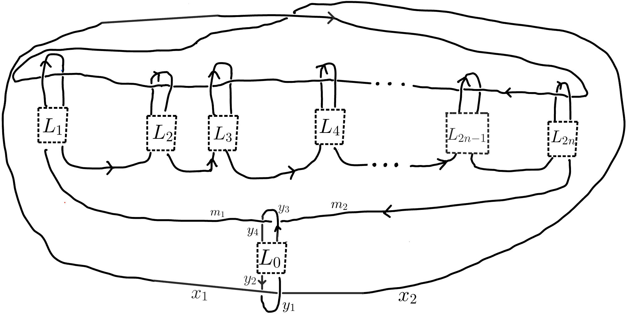
Figure 7.4: A generalization for $A_{n}$. In $A_{n}$, each $L_{i},i>1$ is the same as $T_{i}$ in figure 3.2. But in this more general form, each $L_{i}$ can be any different type $L_{om}$ tangles.

Proof for proposition 7.3 (sketch):
In the proof for general Allen-Swenberg link (section 4.5), we did not use any information for the tangle $L_{p}$($T_{i}$) itself other than lemma 1, which is contains in Theorem 5.1. So for the proof of the link in figure 7.4, since we can apply theorem 5.1 on any $L_{i},i>0$, we can just repeat the proof in section 4.5 for proposition 4.5. In this process we would first derive $m_{1}=m_{2},x_{1}=x_{2}$, then we can by apply theorem 5.1 to $L_{0}$ and easily show that the four crossings in the bottom force $y_{2}=y_{1},y_{3}=y_{4}$ and $x_{1}\sim y_{1}\sim m_{1}$ The first two equations make $L_{0}$ degenerate to an unknot by property 8 in section 5.7. This make it the same condition as for the coloring on $A_{n}$ in section 4.5, so eventually the argument in 4.5 enanbles us to conclude that the solution set associated with the coloring space of the link in 7.4 is has the same form as that of a general Allen-Swenberg link (same as the form concluded in section 4.6), so it cannot be distinguished from $L_{2H}$.

8 Reference

[1]V. Chernov and S. Nemirovski. Legendrian links, causality, and the low conjecture. Geom. Fuct. Anal., 19(0222503):1323–1333, 2010.
[2]R. J. Low. Causal relations and spaces of null geodesics. PhD thesis, Oxford University, 1988.
[3]S.Allen and J.Swenberg. Do link polynomials detect causality in globally hyperbolic space-times? J. Math. Phys., 62(3), 2021.
[4] Miller, Jacob. ”Quandle Invariants of Knots and Links.” (2022).
[5] Nelson, Sam. ”Classification of finite Alexander quandles.” arXiv preprint math/0202281 (2002).
[6] A. Navas and S. Nelson. On symplectic quandles. Osaka J. Math, 45(4):973–985, December 2008.