FQsun: A Configurable Wave Function-Based Quantum Emulator for Power-Efficient Quantum Simulations

Abstract

Quantum computing has emerged as a powerful tool for solving complex computational problems, but access to real quantum hardware remains limited due to high costs and increasing demand for efficient quantum simulations. Unfortunately, software simulators on CPUs/GPUs such as Qiskit, ProjectQ, and Qsun offer flexibility and support for a large number of qubits, they struggle with high power consumption and limited processing speed, especially as qubit counts scale. Accordingly, quantum emulators implemented on dedicated hardware, such as FPGAs and analog circuits, offer a promising path for addressing energy efficiency concerns. However, existing studies on hardware-based emulators still face challenges in terms of limited flexibility, lack of fidelity evaluation, and power consumption. To overcome these gaps, we propose FQsun, a quantum emulator that enhances performance by integrating four key innovations: efficient memory organization, a configurable Quantum Gate Unit (QGU), optimized scheduling, and multiple number precisions. Five FQsun versions with different number precisions, including 16-bit floating point, 32-bit floating point, 16-bit fixed point, 24-bit fixed point, and 32-bit fixed point, are implemented on the Xilinx ZCU102 FPGA, utilizing between 9,226 and 18,093 LUTs, 1,440 and 7,031 FFs, 344 and 464 BRAMs, and 14 and 88 DSPs and consuming a maximum power of 2.41W. Experimental results demonstrate high accuracy in normalized gate speed, fidelity, and mean square error, particularly with 32-bit fixed-point and floating-point versions, establishing FQsun’s capability as a precise quantum emulator. Benchmarking on quantum algorithms such as Quantum Fourier Transform, Parameter-Shift Rule, and Random Quantum Circuits reveals that FQsun achieves superior power-delay product, outperforming traditional software simulators on powerful CPUs by up to $\text{9.87}\times\text{10}^{\text{3}}$ times. Additionally, FQsun shows significantly improved normalized gate speed compared to hardware-based emulators, ranging from 1.31 times to 1.51 $\times\text{10}^{\text{10}}$ times, highlighting its potential as a scalable and energy-efficient solution for advanced quantum simulations.

=-15pt

I Introduction

Quantum computing is captivating research field that has many promising applications in factorial problem [1], searching [2], optimization [3], or quantum machine learning [4]. Numerous researchers have developed real quantum devices successfully, such as IBM Quantum [5], Google Quantum AI [6], and QuEra [7], some even claim to have achieved “quantum supremacy”. Recently, quantum computers have rapidly transformed from the Noise-Intermediate Scale (NISQ) era to the Fault-Tolerant Quantum Computer (FTQC) era, in which the logical error rate from quantum calculations is acceptable. Therefore, it pursued the development of research in quantum computing. However, accessible quantum computers such as IBM quantum computers are limited, because of the high cost of access.

To satisfy the growing demand for quantum computing simulations, several substantial researches have been conducted, as summarized in detail in Table I. Key criteria include physical hardware implementation, benchmarking tasks, the number of simulated qubits (#Qubits), precision, and evaluation metrics. Among existing quantum simulation software development kits (SDKs), the most well-known include Qiskit [8], ProjectQ [9], Cirq [10], and TensorFlow Quantum (TFQ) [11], which are developed in Python. These SDKs not only support a wide range of quantum simulation models with high #Qubits but also enable deployment on actual Quantum Processing Units (QPUs). Additional packages, such as QUBO [12], PennyLane [13], and cuQuantum [14], are also widely used due to their efficient performance on general-purpose processors including Central Processing Units (CPUs) and Graphics Processing Units (GPUs). Notably, cuQuantum is optimized specifically for NVIDIA GPUs. Another notable package is Qsun, a quantum simulation package proposed in [15], which introduces a Wave Function (WF) - based quantum simulation system to reduce the computational load. Overall, these quantum simulation packages exhibit flexible and increasingly fast performance on software platforms. However, as the demand for higher #Qubits grows, the reliance on 32- and 64-bit floating-point (FP) types and the general-purpose design of these software-based quantum simulators result in decreased processing speed and significant storage requirements. Consequently, these platforms tend to consume considerable energy without meeting speed requirements, an issue that is often overlooked in current research. In the future, if quantum simulations become widespread, software quantum simulators running on devices such as CPUs/GPUs, which consume between 150-350 W, will have a significant environmental impact.

To solve the limitations of software, various quantum emulation systems have been developed for hardware platforms, particularly analog circuits and Field-Programmable Gate Arrays (FPGA). Specifically, analog-based emulators, introduced in [16], use CMOS analog circuits to represent real numbers naturally, which are suitable for simulating quantum states. Although analog circuits achieve higher energy efficiency, scalability, and simulation speed than software, they face limitations, when they only support algorithms like Grover’s Search Algorithm (GSA) and Quantum Fourier Transform (QFT) with lower fidelity due to noise and other unintended effects. In contrast, FPGA-based quantum emulators, introduced in [17, 18, 19, 20, 21, 22, 23, 24, 25, 26], offer a more practical and developable approach, while still achieving high speed and energy efficiency. However, these studies lack detailed fidelity evaluations, particularly when using $8$-bit and $16$-bit fixed-point (FX) representations, which may not meet precision requirements. FPGA-based emulators are also limited by high storage and communication demands, restricting them to lower #Qubits. Moreover, these FPGA emulators have low flexibility, as they are optimized only for specific applications such as QFT, GSA, Quantum Haar Transform (QHT), and Quantum Support Vector Machine (QSVM). In general, existing related works continue to face specific challenges, including high energy consumption in quantum simulators, while hardware-based quantum emulators remain limited by low flexibility, reduced precision, and limited applicability due to implementation difficulties. Although they attempt to improve performance, most are constrained by the #Qubit they can simulate and lack detailed evaluations of parameters that reflect accuracy, such as fidelity or mean-square error (MSE). This severely impacts their quality and practicality.

To address the aforementioned challenges, the FQsun quantum emulator is proposed to achieve optimal speed and energy efficiency. FQsun implements four innovative propositions: efficient memory organization, a configurable Quantum Gate Unit (QGU), optimal working scheduling, and multiple number precisions to maximize the flexibility, speed, and energy efficiency of the quantum emulator. FQsun is implemented on a Xilinx ZCU102 FPGA to demonstrate its effectiveness at the real-time SoC level. Through strict evaluation of execution time, accuracy (MSE, fidelity), power consumption, and power-delay product (PDP), FQsun will demonstrate its superiority over software quantum simulators running on powerful Intel CPUs and Nvidia GPUs, as well as existing hardware-based quantum emulators when performing various quantum simulation tasks.

TABLE I: Surveyed results of related quantum simulators/emulators in recent five years

Reference	Devices	Benchmarking tasks	#Qubits	Precision	Comparison metrics
Qiskit [8]	CPUs, GPUs, QPUs	Quantum Fourier Transform (QFT), Bernstein-Vazirani (BV), Random Clifford circuits, Hamiltonian simulation, Quantum Approximate Optimization Algorithm (QAOA)	Depending on hardware resources	32-bit FP, 64-bit FP	Execution time, Gate count, Gate depth, Fidelity
ProjectQ [9]	CPUs, GPUs, QPUs	QFT, Shor’s Algorithm	Depending on hardware resources	32-bit FP, 64-bit FP	Execution time, Resource utilization, Circuit depth, Gate count, Fidelity
Cirq [10]	CPUs, GPUs, QPUs	Random Quantum Circuits (RQC)	Depending on hardware resources	32-bit FP	Execution time, Fidelity
TFQ [11]	CPUs, GPUs, QPUs	QAOA, Quantum Neural Network (QNN).	Depending on hardware resources	32-bit FP, 64-bit FP	Execution time, Fidelity, Gradient-based optimization
QUBO [12]	CPUs, GPUs	QFT, Variational Quantum Eigensolver (VQE), Grover’s Search Algorithm (GSA), Adiabatic Time Evolution, Quantum Autoencoder, Quantum Classifier	Depending on hardware resources	32-bit FP, 64-bit FP	Execution time, Fidelity, Overlap
PennyLane [13]	CPUs, GPUs	VQE, QAOA, Quantum Classification	Depending on hardware resources	32-bit FP, 64-bit FP	Execution time, Fidelity, Variational accuracy
cuQuantum SDK [14]	GPUs	QFT, QAOA, Quantum Volume and Phase Estimation	Depending on hardware resources	32-bit FP, 64-bit FP	Execution time, Speedup factor, Memory bandwidth utilization
Qsun [15]	CPUs	Quantum Linear Regression (QLR), QNN, Quantum Differentiable Programming (QDP)	Depending on hardware resources	32-bit FP, 64-bit FP	Execution time, Fidelity, MSE
Analog-based emulator [16]	UMC-180 nm CMOS Analog	GSA, QFT	6 to 17 qubits	32-bit FP	Execution time, Power consumption, Circuit compatibility
ZCVU9P-based emulator [17]	FPGA(Xilinx ZCVU9P) + CPU(Xeon™ E5-2686 v4)	Quantum Support Vector Machine (QSVM), Quantum Kernel Estimation	Up to 6 qubits	16-bit FX	Execution time, Numerical accuracy, Test accuracy
Alveo-based emulator [18]	FPGA (Xilinx Alveo U250)	Quantum Haar Transform (QHT), 3D-QHT	10 to 32 qubits ($\dagger$)	32-bit FP	Execution time, Resource utilization, Circuit depth
Arria-based emulator [19]	FPGA (Arria 10AX115N4 F45E3SG)	GSA	Up to 32 qubits ($\dagger$)	16-bit FX	Emulation time, Resource utilization, Frequency
XCKU-based emulator [20]	FPGA(Xilinx XCKU115)	QFT	Up to 16 qubits	16-bit FX	Execution time
Stratix-based emulator [21, 22]	FPGA(Altera Stratix EP1S 80B956C6)	QFT, GSA	Up to 8 qubits	8-bit FX, 16-bit FX	Logic cell usage, Emulation time, Frequency
This work FQsun	FPGA(Xilinx ZCU102)	QFT, Parameter - Shift Rule (PSR) (renamed from QDP), RQC, QLR, QNN, etc.	3 to 17 qubits	16-bit FX, 16-bit FP, 24-bit FX, 32-bit FX, 32-bit FP	Execution time, PDP, Fidelity, MSE, Power Hardware Utilization.
${\dagger}$ Qubit numbers marked as ”estimated” are based on projected performance given hardware constraints.

The outline of this paper is organized as follows. Section II presents the background of the study. Next, details of the FQsun hardware architecture are presented in Section III. Then, benchmarking results, evaluation, and comparisons are elaborated upon in Section IV. Finally, Section V concludes the paper.

II Backgrounds

II-A Quantum simulator

Due to the wide range of applications and programming languages, many quantum simulators have been proposed, from low-level languages such as C to high-level languages such as Python. The goals of quantum simulator development range from domain-specific to general purpose, then reach the boundary of quantum advantage where classical computers can no longer simulate a quantum system in acceptable runtime. The basic operation in $n$ (#Qubits)-qubit quantum system can be expressed as:

$$|\psi^{(\bm{m})}\rangle=\mathcal{U}(\bm{\theta})|\psi^{(\bm{0})}\rangle$$ (1)

parameterized by $\bm{\theta}$, where $\mathcal{U}(\bm{\theta})=\bigotimes_{t=1}^{m}U^{(\bm{t})}$ is composed from $\{g_{j}\}_{j=1}^{m}$ and $m$ is the number of quantum gates (gates). $|\psi^{(\bm{t})}\rangle$ is presented by $[\alpha_{0}^{(\bm{t})}\;\alpha_{1}^{(\bm{t})}\;\ldots\;\alpha_{N-1}^{(\bm{t})}]=\sum_{j=0}^{N-1}\alpha_{j}^{(\bm{t})}|j\rangle$ with $|j\rangle$ are elements of the computational basis and $\{\alpha_{j}^{(\bm{t})}\}$ are complex entries ($N=2^{n}$). $\mathcal{U}(\bm{\theta})$ and $|\psi^{(\bm{t})}\rangle$ satisfy unitary and normalize condition, respectively:

$$(U^{(\bm{t})})^{\dagger}U^{(\bm{t})}=\mathbb{I},\;\langle\psi^{(\bm{t})}|\psi^{(\bm{t})}\rangle=1.$$ (2)

The target of simulating quantum computing is to get the expectation value when measuring a final quantum state under a specific observable $\hat{B}:\langle E\rangle=\langle\psi|\hat{B}|\psi\rangle$, which is known as the physical property of the quantum system, summarized as Definition 1.

Definition 1 (Strong and weak simulation)

Given a quantum circuit $U$ and any specified object $x$, the strong simulation can compute any value $\langle\bm{0}|U|x\rangle$ and a weak simulation samples from the distribution $p(x)=|\langle\bm{0}|U|x\rangle|^{2}$ [27, 28].

The term $\mathcal{U}(\bm{\theta})|\psi^{(\bm{0})}\rangle$ can be computed in various approaches mainly by Matrix Multiplication (MM) [29, 30, 14] or WF. In principle, MM conducts vanilla matrix-vector multiplication between operators and state vector, consuming $\mathcal{O}(m\times 2^{2n})$ in time complexity and $\mathcal{O}(2^{2n}+2^{n})$ in space complexity for storing both operator and state vector. MM can be accelerated through some strategies, including gate fusion [31], indexing, realized-state representation [32], sparse matrix calculation, tensor network contraction [33, 34]. The second approach represents quantum circuits using their corresponding WF [9, 35]. The WF approach can, in theory, require only $\mathcal{O}(2^{n})$ in space complexity for storing only state vector, which less computational operations and less temporary memory space for conducting (1).

[t!](topskip=0pt, botskip=0pt, midskip=0pt)[width=0.85]images/overview.pdf Quantum circuit simulation model where it can divide into parameterized and fixed parts, denoted as $U(\bm{\theta})$ and $V$, respectively (both can be notated as $U^{(\bm{t})}$). (Inset left) An example of a parameterized part is the ZXZ layer. (Inset right) An example of a fixed part is the QFT circuit, each part inside consists of many basic gates.

II-B Simulating quantum circuit by wave-function approach

The MM approach operates in two steps. Firstly, $U^{(\bm{t})}$ is constructed by tensor-product between $g_{j}$ and $\mathbb{I}$, later, we conduct MM operation between $U^{(\bm{t})}$ and $|\psi^{(\bm{t-1})}\rangle$, where $U^{(\bm{t})}|\psi^{(\bm{t-1})}\rangle=|\psi^{(\bm{t})}\rangle$. With the unfavorable, $U^{(\bm{t})}\in\mathbb{C}^{N\times N}$, there is an exponential resource scaling of both state vector and operators with increasing $\#\text{Qubits}$.

Instead of constructing a large matrix such as $U^{(\bm{t})}$, The WF approach uses $m$ gates $\{g_{j}\}$ directly, took only $2^{n+\hat{n}_{j}+1}$ multiplication and $2^{n+\hat{n}_{j}+1}$ addition per gate, with $\hat{n}_{j}\in[1,2]$ is the number of operand of the gate $j$; instead of $2^{2n}$ multiplication and $2^{2n-2}$ addition following by MM approach. The idea behind this technique is to update only non-zero amplitudes in $|\psi^{(\bm{t})}\rangle$ sequentially:

$$|\psi^{(\bm{m})}\rangle=\mathcal{W}(g_{m})\ldots\mathcal{W}(g_{2})\mathcal{W}(g_{1})|\psi^{(\bm{0})}\rangle,$$ (3)

where $g\in\mathcal{G}=\{H,S,CX,R_{i}(.)\},i\in\{x,y,z\}$, $\{H,S\}$ and $CX$ are constant $2\times 2$ and $4\times 4$ matrices, respectively. $R_{i}(.)$ is the $2\times 2$ parameterized matrix with single parameter $\theta\in[0,2\pi]$. $\text{Clifford}+R_{i}$ is chosen for two purposes. First, the universal gate set known as Clifford + T belongs to the above set as Definition 2, where the $T$ gate is equivalent to the $R_{z}(\pi/4)$ gate, and the second is that simulating variational quantum model requires the use of parameterized gates.

Definition 2 (Gate set for strong simulation)

Clifford group include $\{H,S,CX\}$ gate which can be used to simulate by the classical algorithm in polynomial time and space, follow Gottesman-Knill theorem [36], which can be extended to Clifford + $R_{i}$.

The transition function $\mathcal{W}(g)$ updates amplitudes $\{\alpha_{j}\}$ directly depending on the type of gate [37], with the acting on the $(w_{0})^{\text{th}}$ qubit as (4):

$$\mathcal{W}(g):\begin{bmatrix}\alpha_{s_{i}}\\ \alpha_{s_{i}+2^{w_{0}}}\end{bmatrix}\rightarrow g\begin{bmatrix}\alpha_{s_{i}}\\ \alpha_{s_{i}+2^{w_{0}}}\end{bmatrix},$$ (4)

where $s_{i}=\lfloor i/2^{w_{0}}\rfloor 2^{w_{0}+1}+\left(i\bmod 2^{w_{0}}\right)$, for all $i\in\left[0,2^{n-1}-1\right]$. We unify the implementation of single- and multiple-qubit gates into a common framework, the operation of single-qubit and $CX$ gates are outlined in Algorithm. 1 and Algorithm. 2, respectively.

Algorithm 1 Operation of a single-qubit gate

$\{\alpha^{(\bm{t})}_{j}\}$, target qubit $w_{0}\in[0,n)$, $g=\begin{bmatrix}a&b\\ c&d\end{bmatrix}\in\mathcal{G}$

$\sum_{j}|\alpha^{(\bm{t})}_{j}|^{2}=1$

$n\leftarrow\log_{2}|\{\alpha_{j}\}|,\text{cut}\leftarrow 2^{n-w_{0}-1}$

$|\psi^{(\bm{t+1})}\rangle=[\alpha^{(\bm{t+1})}_{0}\;\alpha^{(\bm{t+1})}_{1}\;\ldots\;\alpha^{(\bm{t+1})}_{N-1}]^{\intercal}\leftarrow[0\;0\;\ldots\;0]^{\intercal},$

$\text{state}=[\text{bin}(0,n),\text{bin}(1,n),\ldots,\text{bin}(N-1,n)]$ $\triangleright$ $\text{bin}(i,k)$ is the function that represent $i$ by $k$ binary bit,

for $i\leftarrow[0,1,\ldots,N-1]$ do

     if $\text{state}[i][w_{0}]==0$ then

         $\alpha^{(\bm{t+1})}_{i}\leftarrow\alpha^{(\bm{t+1})}_{i}+a\times\alpha^{(\bm{t})}_{i}$

         $\alpha^{(\bm{t+1})}_{i+\text{cut}}\leftarrow\alpha^{(\bm{t+1})}_{i+\text{cut}}+b\times\alpha^{(\bm{t})}_{i}$

     else

         $\alpha^{(\bm{t+1})}_{i}\leftarrow\alpha^{(\bm{t+1})}_{i}+d\times\alpha^{(\bm{t})}_{i}$

         $\alpha^{(\bm{t+1})}_{i-\text{cut}}\leftarrow\alpha^{(\bm{t+1})}_{i-\text{cut}}+c\times\alpha^{(\bm{t})}_{i}$

     end if

end for

return $\{\alpha^{(\bm{t+1})}_{j}\}$

Algorithm 2 Operation of CX gate

$\{\alpha^{(\bm{t})}_{j}\}$, control-target qubits $w_{0},w_{1}\in[0,n)$, $g=\begin{bmatrix}\mathbb{I}&\bm{0}\\ \bm{0}&\mathbb{X}\end{bmatrix}\in\mathcal{G}$

$\sum_{j}|\alpha^{(\bm{t})}_{j}|^{2}=1$

$n\leftarrow\log_{2}|\{\alpha_{j}\}|,\text{cut}\leftarrow 2^{n-w_{1}-1}$

$|\psi^{(\bm{t+1})}\rangle=[\alpha^{(\bm{t+1})}_{0}\;\alpha^{(\bm{t+1})}_{1}\;\ldots\;\alpha^{(\bm{t+1})}_{N-1}]^{\intercal}\leftarrow[0\;0\;\ldots\;0]^{\intercal},$

$\text{state}=[\text{bin}(0,n),\text{bin}(1,n),\ldots,\text{bin}(N-1,n)],$

for $i\leftarrow[0,1,\ldots,N-1]$ do

     if $\text{state}[i][w_{0}]==1$ then

         if $\text{state}[i][w_{1}]==1$ then

              $\alpha^{(\bm{t+1})}_{i-\text{cut}}\leftarrow\alpha^{(\bm{t+1})}_{i-\text{cut}}+\alpha^{(\bm{t})}_{i}$

         else

              $\alpha^{(\bm{t+1})}_{i+\text{cut}}\leftarrow\alpha^{(\bm{t+1})}_{i+\text{cut}}+\alpha^{(\bm{t})}_{i}$

         end if

     else

         $\alpha^{(\bm{t+1})}_{i}\leftarrow\alpha^{(\bm{t})}_{i}$

     end if

end for

return $\{\alpha^{(\bm{t+1})}_{j}\}$

II-C Preliminary Challenges for Developing a High Efficiency Quantum Emulator

To develop a quantum emulator that meets the demands of speed, flexibility, and energy efficiency, several core challenges must be addressed. Each of these challenges highlights essential requirements that drive the need for innovative design improvements in quantum emulation systems:

• Efficient Memory Management: Quantum emulation requires managing and processing large datasets, especially as the number of qubits increases, which dramatically expands memory demands. Efficient data handling and minimized memory access times are crucial to achieving high processing speeds without excessive energy consumption.

• Flexible Quantum Gate Configuration: Different quantum algorithms rely on a variety of quantum gates, but many emulators are constrained by limited gate support. To effectively execute diverse algorithms, an adaptable gate configuration system is needed to facilitate a wide range of quantum computations with minimal hardware reconfiguration.

• Optimized Task Scheduling: Quantum emulators must execute sequential calculations, where delays in one step can impact the entire system’s performance. To avoid bottlenecks, the emulator requires an optimized scheduling mechanism to ensure continuous, efficient processing without latency, thus maximizing resource utilization and overall computation speed.

• Multi-Level Precision Support: Quantum algorithms often demand different levels of numerical precision, from FX to FP, depending on application requirements. Supporting various precision levels allows the emulator to balance accuracy with resource usage, adapting performance to meet the specific needs of each quantum task while minimizing computational overhead.

Each of these challenges underscores the necessity of a robust, scalable emulator that can dynamically adjust to complex quantum workloads while maintaining efficiency and precision across diverse applications.

III Proposed Architecture

III-A System Overview Architecture

TABLE II: Supported gates on FQsun, including Clifford + $R_{i}$ set with additional gates $\{T,X,Y,Z\}$.

Gate	Matrix Representation	Parameter	Equivalent to
$H$	$\frac{1}{\sqrt{2}}\begin{bmatrix}1&1\\ 1&-1\end{bmatrix}$	$w_{0}$	Basic gate
$S$	$\begin{bmatrix}1&0\\ 0&i\end{bmatrix}$	$w_{0}$	Basic gate
$CX$	$\begin{bmatrix}1&0&0&0\\ 0&1&0&0\\ 0&0&0&1\\ 0&0&1&0\end{bmatrix}$	$w_{0},w_{1}$	Basic gate
$R_{x}(\theta)$	$\begin{bmatrix}\cos\left(\frac{\theta}{2}\right)&-i\sin\left(\frac{\theta}{2}\right)\\ -i\sin\left(\frac{\theta}{2}\right)&\cos\left(\frac{\theta}{2}\right)\end{bmatrix}$	$w_{0},\theta$	Basic gate
$R_{y}(\theta)$	$\begin{bmatrix}\cos\left(\frac{\theta}{2}\right)&-\sin\left(\frac{\theta}{2}\right)\\ \sin\left(\frac{\theta}{2}\right)&\cos\left(\frac{\theta}{2}\right)\end{bmatrix}$	$w_{0},\theta$	Basic gate
$R_{z}(\theta)$	$\begin{bmatrix}e^{-i\frac{\theta}{2}}&0\\ 0&e^{i\frac{\theta}{2}}\end{bmatrix}$	$w_{0},\theta$	Basic gate
$T$	$\begin{bmatrix}1&0\\ 0&e^{-i\pi/4}\end{bmatrix}$	$w_{0}$	$R_{z}(\pi/4)$
$X$	$\begin{bmatrix}0&1\\ 1&0\end{bmatrix}$	$w_{0}$	$R_{x}(\pi)$
$Y$	$\begin{bmatrix}0&-i\\ i&0\end{bmatrix}$	$w_{0}$	$R_{y}(\pi)$
$Z$	$\begin{bmatrix}1&0\\ 0&-1\end{bmatrix}$	$w_{0}$	$R_{z}(\pi)$

Fig. III-A details the proposed FQsun architecture on an FPGA at the system-on-chip (SoC) level. The system comprises four components: Qsun Framework, FQsun Software, Processing System (PS), and FQsun in Programmable Logic (PL).

The Qsun Framework, implemented in Python, includes libraries and programs for quantum simulation. These programs can instruct the hardware to execute gates through the FQsun C library in FQsun Software. Users proficient in C programming can directly write C programs by calling quantum circuits defined in the FQsun library to achieve higher performance. Within the PS, the embedded CPU runs software such as the Qsun Framework and FQsun Software to control FQsun in PL for executing quantum simulation tasks. In the PL, the proposed FQsun consists of four modules: AXI Mapper, memory system, FQsun controller, and QGU. The AXI Mapper manages and routes data exchanged between the PS and the FQsun memory system. The FQsun memory system comprises Control Buffers, Context Memory, and a pair of Ping/Pong Amplitude Memory modules. Control Buffers store control signals for the host FQsun Controller. Context Memory holds configuration information such as gate type, gate location ($cut$, $\sin(\theta/2)$, $\cos(\theta/2)$, $w_{0}$, $w_{1}$), and gate parameters. Notably, the Ping/Pong Amplitude $2\times 2048$ (KB) Memory is the largest memory unit designed to store $\{\alpha^{(t)}_{j}\}$ for QGU. Finally, QGU serves as the main processing unit of FQsun. QGU contains six fundamental gate units: $\{H,S,CX,R_{x},R_{y},R_{z}\}$. These basic gates can be combined to implement most other gates, ensuring high flexibility. The system overview architecture is designed to ensure compatibility between the PS and FQsun in hardware for stable and optimal operation. By supporting the FQsun library in Python and C, users can easily utilize FQsun to perform quantum tasks. The next section will detail the memory system optimization of FQsun.

[t!](topskip=0pt, botskip=0pt, midskip=0pt)[width=.99]images/SoC_Overview.pdf Overview architecture of our FQsun at the system-on-chip (Soc) level on FPGA.

III-B Efficient Memory Organization

As mentioned in Section II-C, matrix size $N$ grows exponentially with $\#\text{Qubits}$ that the emulator supports. Meanwhile, hardware platforms such as FPGAs are limited by storage resources. To support large $\#\text{Qubits}$, the memory organization of FQsun must be optimized. Fig. III-B illustrates the memory organization of the proposed FQsun for efficient operation on FPGA. There are three types of memory: Control Buffers, Context Memory, and Ping/Pong Amplitude Memory.

Control Buffers: These buffers store 1-bit control signals such as load, start, done, and stop. The load signal is used by the host to indicate the state where it writes context and amplitude data. Additionally, the host uses a 5-bit signal to indicate $\#\text{Qubits}$, that FQsun is supporting. After completing the load state, the host triggers the start signal to begin the session. The done signal is continuously read by the host to track the completion time of each gate operation. Finally, the stop signal is used to end the session by resetting the address register of the Context Memory.

Context Memory ($\bm{16}$ KB): This memory stores configuration data for FQsun and has $d=2048$. The configuration data includes a $3$-bit gate opcode indicating the type of gate to be executed. The values $\sin(\theta/2)$ and $\cos(\theta/2)$, with a bit width of $16/24/32$ depending on the precision type, are parameters for $R_{i}$, pre-computed by FQsun software to reduce hardware complexity. Additionally, parameters such as the $5$-bit cut and gate positions $\{w_{0},w_{1}\}$ must also be stored. With this Context Memory design, FQsun can support the execution of up to $2048$ gates in a computational sequence.

Ping/Pong Amplitude Memory ($\bm{2}$ MB): This is the largest memory and is used to store $\{\alpha^{(\bm{t})}_{j}\}$ for QGU. This memory must have a $d=2^{18}$ to support up to $18$ qubits, calibrated to fit the maximum BRAM capacity of the Xilinx ZCU102 FPGA. In case, Ping/Pong Amplitude Memory is applied to FPGAs with more abundant BRAM resources, such as the Alveo or Versal series, FQsun could support a larger $\#\text{Qubits}$. To enable amplitude updates as described in Algorithms 1 and 2, a dual-port Ping/Pong memory design is applied. Specifically, if the ping memory holds the current amplitude $\{\alpha^{(\bm{t})}_{j}\}$, the pong memory will store the new amplitude $\{\alpha^{(\bm{t+1})}_{j}\}$, and vice versa. This design is essential on the grounds that, during the calculation of $\{\alpha^{(\bm{t+1})}_{i+cut}\}$ and $\{\alpha^{(\bm{t+1})}_{i-cut}\}$, both the current and new amplitudes are needed. The use of Ping/Pong memory allows for continuous amplitude updates, thereby optimizing simulation performance.

[t!](topskip=0pt, botskip=0pt, midskip=0pt)[width=.99]images/Memory_Organization.pdf Memory organization of the proposed FQsun.

Overall, with its efficient memory organization, FQsun ensures support for quantum emulation with a large $\#\text{Qubits}$ and various gate types, optimizing both performance and flexibility. The next section provides detailed information on the architecture of the configurable QGU to explain how FQsun supports multiple gate types.

III-C Configurable Quantum Gate Unit (QGU)

[t!](topskip=0pt, botskip=0pt, midskip=0pt)[width=.99]images/QGU.pdf Micro-architecture of QGU.

Currently, existing quantum emulators on hardware face difficulties in supporting a wide variety of quantum simulation applications. This challenge arises due to the limited flexibility of their computational hardware architectures in executing complex gates critical for many applications, thereby restricting their capabilities. Consequently, the QGU hardware architecture is proposed to enable FQsun to achieve the highest level of flexibility in supporting any quantum simulation applications.

The micro-architecture of the QGU, as detailed in Fig. III-C, consists of five main modules designed to perform six fundamental gates ($\mathcal{G}$) in Table II, following software design. The computational data for the QGU includes $\{\alpha^{(\bm{t})}_{i}\}$, $\{\alpha^{(\bm{t+1})}_{i}\}$, $\{\alpha^{(\bm{t+1})}_{i\pm cut}\}$, and parameters ($\sin(\theta/2)$ and $\cos(\theta/2)$) used by $R_{i}$. Essentially, the operations of $R_{x}$ and $R_{y}$ are relatively similar; hence, they are implemented using a Unified $R_{x}$ & $R_{y}$ Gate unit to conserve hardware resources. To ensure proper execution of the if-else logic as outlined in Algorithms. 1 & 2, a 2-to-1 multiplexer system controlled by the state value is used to select the output value. Finally, a multiplexer controlled by the Gate operation input is employed. By combining the fundamental gates to form other gates, the QGU can be configured to execute all gates utilized by Qsun[15], enabling diverse quantum applications. Moreover, to ensure the highest operating frequency, the operators within the quantum gate modules, such as multiplication and addition, are pipelined to shorten the critical path. Specifically, for FP numbers, multiplication and addition each require two stages, while for FX numbers, multiplication requires two stages, and addition does not require any stage.

In summary, the proposed QGU design optimizes hardware flexibility and efficiency. The following section will provide a detailed discussion of the timing schedule for an FQsun session at the SoC level.

III-D Optimal working scheduling

[t!](topskip=0pt, botskip=0pt, midskip=0pt)[width=.99]images/Working_Flow.pdf Timing chart of our FQsun operation using ping/pong amplitude memories.

When operating at the SoC level, without a well-defined timing schedule for read and write operations in the memory system, FQsun cannot operate efficiently due to various issues, such as incorrect timing for control signal transmission when the computational data is not available or incorrect data read/write in the Ping/Pong Amplitude Memory.

To address these issues, the timing diagram of FQsun for executing a working session is detailed in Fig. III-D. At the beginning of a session, context data is stored in the Context Memory, which contains configuration commands for FQsun to execute a quantum circuit consisting of $m$ gates for a specific application. Next, the system writes initial amplitudes $\{\alpha^{(\bm{0})}_{j}\}$ into the Ping Amplitude Memory. The read/write process for amplitude data incurs the highest memory access time because the amplitude vector is large ($N=2^{n}$). Once the ping memory is fully loaded with data, the system sends a control signal to initiate the FQsun working session. An internal control register called the Program Counter (PC) is used to track the instruction index to determine the current gate for execution. After reading the instruction from the Context Memory at address $\text{PC}=0$, QGU loads the initial amplitude data $\{\alpha^{(\bm{0})}_{j}\}$ from Ping Amplitude Memory and the initial new amplitude data $\{\alpha^{(\bm{1})}_{j}\}$ from Pong Amplitude Memory. This data is processed by Gate 0 in N iterations to produce the updated new amplitude $\{\alpha^{(\bm{0})}_{j}\}$, increment the PC for the next instruction, and clear the data in Ping Memory (new initial amplitude is zero). At $\text{PC}=1$, QGU proceeds to read the context of Gate 1, read amplitude $\{\alpha^{(\bm{1})}_{j}\}$ from Pong Amplitude Memory, and new amplitude $\{\alpha^{(\bm{2})}_{j}\}$ from Ping Amplitude Memory. After executing and storing the updated amplitude $\{\alpha^{(\bm{2})}_{j}\}$ in Ping Amplitude Memory, the PC is incremented by 1, and Pong Amplitude Memory is cleared. This alternating process continues, updating the new amplitude data and storing it in Ping/Pong Amplitude Memory with each gate execution. Throughout FQsun’s computation, the host PS continuously reads and checks the Done flag to determine when the hardware has completed its task. Accordingly, the host PS reads the final amplitude $\{\alpha^{(\bm{m})}_{j}\}$ from Pong Amplitude Memory if $m$ is odd, and from Ping Amplitude Memory if $m$ is even.

Typically, FQsun’s working schedule makes sure that the host PS accurately and successfully runs FQsun’s session. In order to minimize latency across the hardware, FQsun simultaneously runs continuously by alternating updates between Ping and Pong Amplitude Memory. The next section will examine five different numerical precision types and identify which ones work well with FQsun in order to maximize hardware accuracy and efficiency.

III-E Multiple number precisions

TABLE III: Preliminary analysis of five suitable number precisions for FQsun

Number Format	Pipeline stages	Range (Precision)	Complexity
FP16 (1-bit sign, 5-bit exponent, 10-bit mantissa)	two for multiplier, two for adder/subtr.	[$6.1\times 10^{-5}$, $6.6\times 10^{-4}$] with 10-bit precision	High due to 5-bit exponent 10-bit mantissa handling
FP32 (1-bit sign, 8-bit exponent, 23-bit mantissa)	two for multiplier, two for adder/subtr.	[$1.2\times 10^{-38}$, $3.4\times 10^{38}$] with 23-bit precision	Higher due to 8-bit exponent, 23-bit mantissa handling, normalization, and rounding
FX16 (1-bit sign, 1-bit integer, 14-bit fractional)	two for multiplier, one for adder/subtr.	[-1, 1] with 14-bit precision ($6.10\times 10^{-5}$)	Lower complexity, only integer-based arithmetic with fixed operators
FX24 (1-bit sign, 1-bit integer, 22-bit fractional)	two for multiplier, one for adder/subtr.	[-1, 1] with 22-bit precision ($2.38\times 10^{-7}$)	Lower complexity, similar to FX16 but with finer precision due to additional fractional bits
FX32 (1-bit sign, 1-bit integer, 30-bit fractional)	two for multiplier, one for adder/subtr.	[-1, 1] with 30-bit precision ($9.31\times 10^{-10}$)	Lower complexity, similar to FX24 but with finer precision due to additional fractional bits

The use of various numerical precisions significantly impacts accuracy, hardware resources, and execution speed. Unfortunately, almost all related work on quantum emulators has primarily focused on performance evaluation while lacking detailed criteria for accuracy metrics such as fidelity or MSE.

In this study, FQsun is designed with five configurations, each corresponding to a different numerical precision: 16-bit floating point (FP16), 32-bit floating point (FP32), 16-bit fixed point (FX16), 24-bit fixed point (FX24), and 32-bit fixed point (FX32). A preliminary comparison of the architectures, number of pipeline stages, range, and complexity is shown in Table III. The following discussion elaborates on the key considerations:

• Pipeline and Complexity: FP numbers utilize two pipeline stages for both the multiplier and the adder/subtractor units, while FX numbers require only two stages for the multiplier and one stage for the adder/subtractor. Moreover, FP operation modules are more complex due to the need to handle exponent, mantissa, normalization, and rounding operations. In contrast, FX operations are simpler and involve integer-based arithmetic with fixed multipliers, adders, or subtractors. As a result, the latency of FX design is lower compared to FP design.

• Range and Precision: following normalize condition in (2), $|\alpha_{j}^{(\bm{t})}|\in[-1,1]$, therefore, FX numbers used in FQsun are configured with $1$ sign bit, $1$ integer bit, and the remaining bits allocated to the fractional part to optimize precision. Although FP numbers offer a higher maximum precision compared to FX numbers, they come at the cost of increased hardware resources and execution time. It is essential to consider the required accuracy for quantum applications to determine the most appropriate numerical precision.

Overall, FP numbers provide higher accuracy but incur higher latency and resource consumption, while FX numbers offer lower accuracy with reduced hardware resource usage and latency. To identify the most suitable configuration, detailed measurements will be conducted in the following section.

IV Verification and results

To verify our proposed design, the below quantum tasks in Section IV-A are used. Through the metrics in Section IV-B, we compared our proposal with CPU, GPU, and other FPGA designs in the rest of this section.

IV-A Tasks used for benchmarking

We chose three tasks to benchmark our proposed emulator with #Qubits from $3$ to $17$. They are motivated by the quantum machine learning model [38, 4], including the Random Quantum Circuits (RQC) sampling [6], quantum differentiable with Parameter-Shift Rule (PSR) technique [39], and the Quantum Fourier Transform (QFT) as a core algorithmic component to many applications [40]. When QFT is one of the standard algorithms for benchmarking the performance of quantum simulators and emulators, we test RQC to know how the universal proposed hardware. Finally, PSR is the most popular technique used in the quantum learning model. In Fig. 1, we illustrate the gate distribution after transpiling the original circuit by the Clifford+$R_{i}$ set. The scaling of $\#\text{gates}$ is polynomial complexity based on $\#\text{Qubits}$. The quantum circuit presentation of the PSR and QFT are shown in Fig. 1 (left) and (right), respectively. Where the circuit sampling from RQC is the combination of used gates with the smallest depth ($d$).

IV-A1 Random Quantum Circuits (RQC)

The pseudo - RQC is a popular benchmarking problem for quantum systems, the problem was first implemented on the Sycamore chip to prove quantum supremacy. The quantum circuit is constructed gate-by-gate by randomly choosing from a fixed pool and designed to minimize the circuit depth. The sequences of gates $\{g_{j}\}$ create a “supremacy circuit” with high classical computational complexity. The RQC dataset from [6] provided the quantum circuit up to $53$ qubits, $1,113$ single-qubit gates, and $430$ two-qubit gates, then proved that the quantum computer can perform this task in seconds (s) instead of a thousand years on classical computers. However, this dataset is fixed, which limits the user when they want to benchmark on different cases. Based on our previous work [41], we generated a bigger RQC dataset, which used an extendable gate pool and different circuit construction strategies. The size of the generated dataset is $14$ GB of $15,000$ random circuit with $d\in[1,10]$ and #Qubits values.

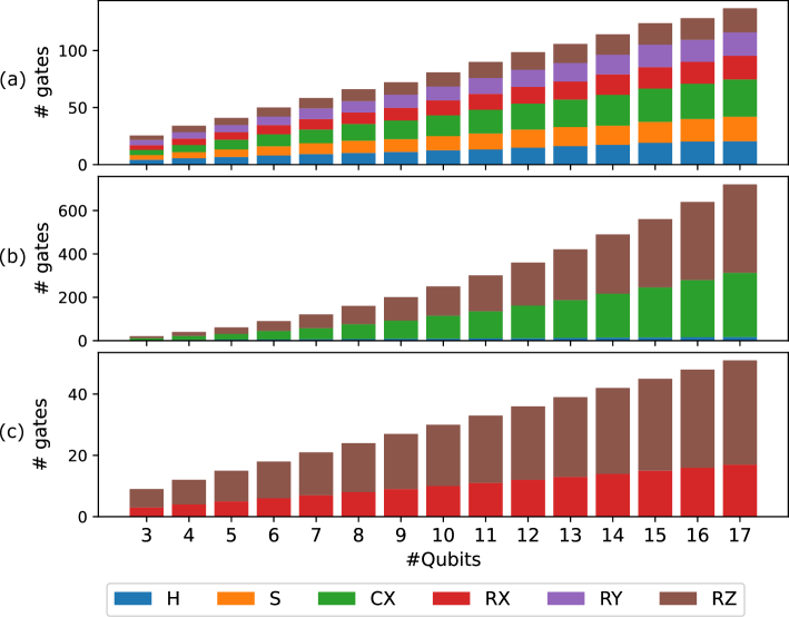
Figure 1: Gate distribution for three benchmarking tasks: (a) RQC (b) QFT and (c) PSR.

IV-A2 Quantum Fourier Transform

Quantum Fourier Transform (QFT) [42] is an important component in many quantum algorithms, such as phase estimation [43], order-finding and factoring [44]. QFT circuit is utilized from Hadamard ($H$), controlled phase ($CP(\theta)$), and SWAP gates where $CP(\theta)$ and SWAP can be decomposed into $R_{z}(\theta)$ and $CX$ gates. These gates transform on an orthonormal basis $\{|0\rangle,\ldots,|N-1\rangle\}$ with the below action on the basis state:

$$|j\rangle\rightarrow\frac{1}{\sqrt{N}}\sum_{k=0}^{N-1}e^{2\pi ijk/N}$$ (5)

If the state $|j\rangle$ is written by using the $n$-bit binary representation $j=j_{1}...j_{n}$:

$$\begin{split}&\text{QFT}(|j_{1},\ldots,j_{n}\rangle)\rightarrow\\ &\frac{(|0\rangle+e^{2\pi i0.j_{n}}|1\rangle)\otimes\ldots\otimes(|0\rangle+e^{2\pi i0.j_{1}j_{2}\ldots j_{n}}|1\rangle)}{\sqrt{N}}\end{split}$$ (6)

where $0.j_{l}\ldots j_{n}=j_{l}/2+\ldots+j_{n}/2^{n-l+1}$. We apply the QFT on the zero state $|\bm{0}\rangle$, which should return the exact equal superposition of all possible $n$-qubit states, means $\alpha_{j}=\alpha_{k}\;\forall j,k\in[0,N)$.

IV-A3 Quantum differentiable programming (QDP) with Parameter-Shift Rule (PSR)

In various quantum learning models, starting with a parameterized quantum circuit $U(\bm{\theta})$, we try to optimize some associated cost value $C(\bm{\theta})$ as (7), which is known as the target of the optimization process by some first-order optimizer such as Gradient Descent (GD), for example, defined as (8):

Task	RQC	QFT	PSR
Gate	Clifford+$R_{i}$	$H,CX,R_{z}$	$R_{x}$,$R_{z}$
Output	$\{|\alpha|^{2}\}$	$\{|\alpha|^{2}\}$	$\{\bm{\theta}^{(\bm{t+1})},|\alpha|^{2}\}$
$\#\text{Gates}$	$~{}n\times d$	$n\;(H)$ $(n+3)(n-1)\;(CX)$ $\frac{3}{2}n(n-1)\;(R_{z})$	$2n\;(R_{z})$ $n\;(R_{x})$

TABLE IV: Properties of benchmarking tasks with different gate types and #Gate.

$$C(\bm{\theta})=\sum_{j=0}^{N-1}j|\alpha_{j}|^{2}$$ (7)

$$\bm{\theta}_{j}^{{}^{\prime}}\leftarrow\bm{\theta}_{j}-\gamma\nabla_{\bm{\theta}}C(\bm{\theta})$$ (8)

where $\bm{\theta}$ is initialized as $[1\;1\;\ldots\;1]^{\intercal}$ and updated sequentially by the general PSR technique [39]. Because the parameterized gate set is limited as a one-qubit rotation gate, only 2-term PSR is used. The gradient is notated as $\nabla_{\bm{\theta}}C(\bm{\theta})=\{\partial_{\theta_{j}}C(\bm{\theta})\}_{j=0}^{m-1}$ and partial derivative $\partial_{\theta_{j}}C(\bm{\theta})$ is presented in (9) with $\bm{e}_{j}$ is the $j^{\text{th}}$-unit vector:

$$\partial_{\theta_{j}}C(\bm{\theta})=\frac{1}{\sqrt{2}}[C(\bm{\theta}+\frac{\pi}{2}\bm{e}_{j})-C(\bm{\theta}-\frac{\pi}{2}\bm{e}_{j})]$$ (9)

The optimal parameter $\bm{\theta}^{*}$ can be obtained through $2m\times n_{\text{iter}}$ quantum evaluations after $n_{\text{iter}}$ iterations.

IV-B Comparison metrics

Essentially, using the proposed simulators without knowledge about their metrics, such as error rate and execution time, can lead to bias during the experiment. Therefore, we propose two type of metrics: accuracy for reliability and performance for comparison between FQsun and other emulators/simulators.

Accuracy metrics: As mentioned in Section II, the target of the quantum emulator is to simulate the transition function $\mathcal{W}(g_{j})$, receives $|\psi^{(\bm{t-1})}\rangle$ and returns $|\psi^{(\bm{t})}\rangle$. To measure the similarity between computational states $\rho$ and theoretical state $\sigma$, trace fidelity, trace infidelity, and trace distance are popularly used, defined in (10), (11) and (12), respectively:

$$\mathcal{F}(\rho,\sigma)=\left(\text{Tr}(\sqrt{\sqrt{\rho}\sigma\sqrt{\rho}})\right)^{2}$$ (10)

$$I\mathcal{F}(\rho,\sigma)=1-\mathcal{F}(\rho,\sigma)$$ (11)

$$\mathcal{T}(\rho,\sigma)=\frac{1}{2}|\rho-\sigma|$$ (12)

Since computing the square root of a positive semi-definite matrix consumes a lot of resources, (10) can be reduced to $\mathcal{F}(\rho,\sigma)=\left|\left\langle\psi_{\rho}\mid\psi_{\sigma}\right\rangle\right|^{2}$ for $\rho=\left|\psi_{\rho}\right\rangle\left\langle\psi_{\rho}\right|$ and $\sigma=\left|\psi_{\sigma}\right\rangle\left\langle\psi_{\sigma}\right|$. $\mathcal{F}(\rho,\sigma)=1$ means $\rho\equiv\sigma$.

TABLE V: Utilization of FQSun on ZCU102 FPGA throughout five designs

Design	Name	LUTs	FFs	BRAM	DSP
FP16	Buffers & AXI Mapper	268	290	0	0
	Context Memory	4,428	0	0	0
	Ping & Pong Memories	3,071	36	464	0
	QGU	5,530	2,752	0	44
	FQsun Controller	937	973	0	0
	Total	14,234	4,051	464	44
FP32	Buffers & AXI Mapper	295	327	0	0
	Context Memory	6,556	0	0	0
	Ping & Pong Memories	3,796	36	456	0
	QGU	6,258	5,296	0	88
	FQsun Controller	1,188	1,372	0	0
	Total	18,093	7,031	456	88
FX16	Buffers & AXI Mapper	264	289	0	0
	Context Memory	4,387	0	0	0
	Ping & Pong Memories	3,168	36	464	0
	QGU	457	142	0	14
	FQsun Controller	990	973	0	0
	Total	9,266	1,440	464	14
FX24	Buffers & AXI Mapper	272	307	0	0
	Context Memory	5,722	0	0	0
	Ping & Pong Memories	3,086	24	344	0
	QGU	684	206	0	28
	FQsun Controller	939	828	0	0
	Total	10,703	1,635	344	28
FX32	Buffers & AXI Mapper	297	327	0	0
	Context Memory	6,888	0	0	0
	Ping & Pong Memories	3,934	36	456	0
	QGU	914	326	0	56
	FQsun Controller	1,136	1,372	0	0
	Total	13,169	2,061	456	56

Since there are a limited number of decimals on the quantum emulator, it makes the systematic error on amplitudes $\{\alpha_{j}\}$ increase as system size. Because $|\{\alpha_{j}\}|=2^{n}$ and $\sum_{j}|\alpha_{j}|^{2}=1$, then $\mathbb{E}[\alpha_{j}]=1/2^{n}$ decrease exponentially based on #Qubits. MSE is calculated as (13) to get the accumulated error of all amplitudes:

$$\text{MSE}(|\psi_{\rho}\rangle,|\psi_{\sigma}\rangle)=\frac{1}{2^{n}}\left(\sum_{j}|\alpha_{j}^{\rho}-\alpha_{j}^{\sigma}|^{2}\right)$$ (13)

Performance metrics: The novelty of FQsun is the high performance, measured via execution time, PDP, and memory efficiency. The execution time (t) is counted by creating a quantum circuit to receive amplitudes. PDP is simply equal to Power $(p)\times t$. When the designed quantum emulator consumes extra-low power compared with CPU/GPU, this metric is important for verifying the performance of FQsun.

IV-C Implementation and Resource Utilization on FPGA

TABLE VI: Basic quantum gate’s period and corresponding #Cycle on FQsun

Version	Period (ns)	#Cycle / Gate
		$H$	$S$	$CX$	$R_{x}$	$R_{y}$	$R_{z}$
FP16	$6.66$	$6$	$4$	4	$6$	$6$	$8$
FP32	$7.35$	$6$	$4$	$4$	$6$	$6$	$8$
FX16	$7.35$	$4$	$2$	$2$	$4$	$4$	$4$
FX24	$8$	$4$	$2$	$2$	$4$	$4$	$4$
FX32	$9.35$	$4$	$2$	$2$	$4$	$4$	$4$

The FQsun design was implemented using Verilog HDL and realized on a 16nm Xilinx ZCU102 FPGA, utilizing Vivado 2021.2 to obtain synthesis and implementation values. The system underwent testing through five FQsun designs with varying precision: FX16, FX24, FX32, FP16, and FP32. The following notation will be for different set of versions: Software = $\{$PennyLane, Qiskit, ProjectQ, Qsun$\}$, FQsun = $\{$FP16, FX32, FX16, FX24, FX32$\}$ and $\text{{FQsun}}^{*}$ = $\{$FP32, FX32, FX24$\}$.

Subsequently, three primary applications as described in Section IV-A were implemented to demonstrate computational efficiency and high flexibility. System accuracy across each design will be recognized by considering $\mathcal{F}$ and MSE values. Consequently, the efficiency and practicality of each FQsun quantum emulator design will be clearly illustrated, alongside detailed presentations of quantum simulator packages on powerful CPUs. Table V provides a detailed report on the utilization of the five FQsun designs when implemented on the Xilinx ZCU102 FPGA, based on the number of lookup tables (LUTs), flip-flops (FFs), Block RAMs (BRAMs), and digital signature processors (DSPs). Accordingly, the designs utilize between 9,226 and 18,093 LUTs, 1,440 to 7,031 FFs, 344 to 464 BRAMs, and 14 to 88 DSPs. It should be noted that the FP16 and FX16 versions exhibit the highest BRAM utilization due to their capacity to accommodate up to 18 qubits. Conversely, the remaining configurations (FQsun^∗) support a maximum of $17$ qubits, resulting in a reduced BRAM requirement. Obviously, the significantly lower DSP utilization compared to FP numbers demonstrates that applying FX numbers to the FQsun emulator results in greater power efficiency. This is because each DSP can be equivalent to multiple LUTs in terms of implementation.

Overall, FX32 utilizes the most LUTs. FP32 utilizes the most FFs and the most DSPs. FX16 and FP16 utilize the least resources. Additionally, all FQsun versions are designed to not utilize DSPs to conserve hardware resources. The subsequent section proceeds to evaluate the MSE of the designs to assess the accuracy of each design.

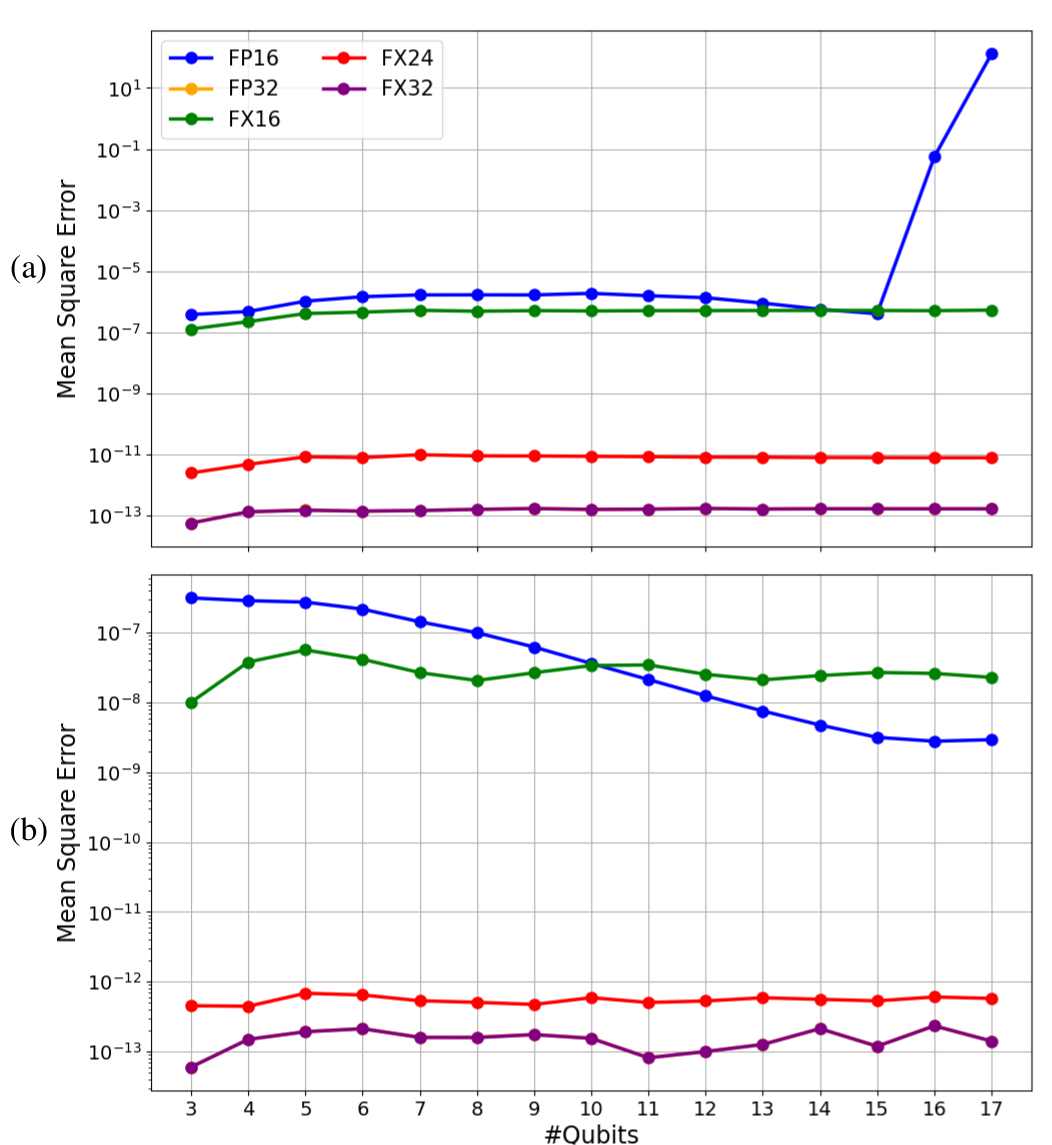
Figure 2: $\text{MSE}_{\text{{FQsun}}}$ on (a) QFT and (b) PSR emulation.

IV-D Gate speed

The gate speed’s properties are presented as Table VI, the execution time per gate is $\text{Period}_{\text{version}}\times\#\text{Cycle}\times 2^{n}$ for looping through amplitudes, which depends on version, gate type, and #Qubits, respectively. These results highlight the trade-off between precision and speed across different versions. For example, while the FP16 version has the shortest period of $6.66$ ns, the FX32 version requires a longer period of $9.35$ ns to execute a gate, reflecting the additional time needed to achieve higher precision. Furthermore, the FX versions generally require fewer cycles per gate compared to FP versions, with reductions ranging from $1.5$ to $2$ times depending on the gate type. For example, the $CX$ gate requires $4$ cycles in FX16 but 6 cycles in FP16, a difference that becomes critical in high-speed applications. This efficiency in FX versions could be advantageous in time-sensitive quantum computations, where lower #Cycles allow for faster gate operations while maintaining adequate precision. Therefore, depending on the application, a balance between speed (fewer #Cycles) and accuracy (higher precision) can be strategically chosen to optimize performance.

IV-E MSE real-time evaluation

To demonstrate the correctness, MSE of the five FQsun designs when performing the QFT and PSR emulators on the real-time ZCU102 FPGA system was measured as shown in the two graphs in Fig. 2. Based on the analyzed data, the designs FQsun^∗ exhibit the lowest MSE values, making them the most suitable candidates for use in quantum emulation. Specifically, FP32 and FX32 demonstrate extremely low MSE values ranging from $5.686\times 10^{-14}$ to $1.656\times 10^{-13}$, indicating greatly high accuracy. FX24 also shows acceptable MSE values, ranging from $2.481\times 10^{-12}$ to $7.798\times 10^{-12}$, which are sufficient for large quantum applications like QFT. In contrast, FP16 and FX16 do not meet the required accuracy standards. FP16 displays significantly high MSE values, with MSE reaching $0.055$ at $\#\text{Qubits}=16$ and spiking to $129.824$ at $\#\text{Qubits}=17$, rendering it unsuitable for precise quantum applications. Similarly, FX16 shows higher MSE values, ranging from $1.278\times 10^{-7}$ to $5.327\times 10^{-7}$, which are inadequate for applications demanding high precision. Thus, the three designs (FQsun^∗) with the lowest MSE: FX24, FP32 and FX32, will be considered for comparison in the subsequent section.

IV-F Fidelity evaluation

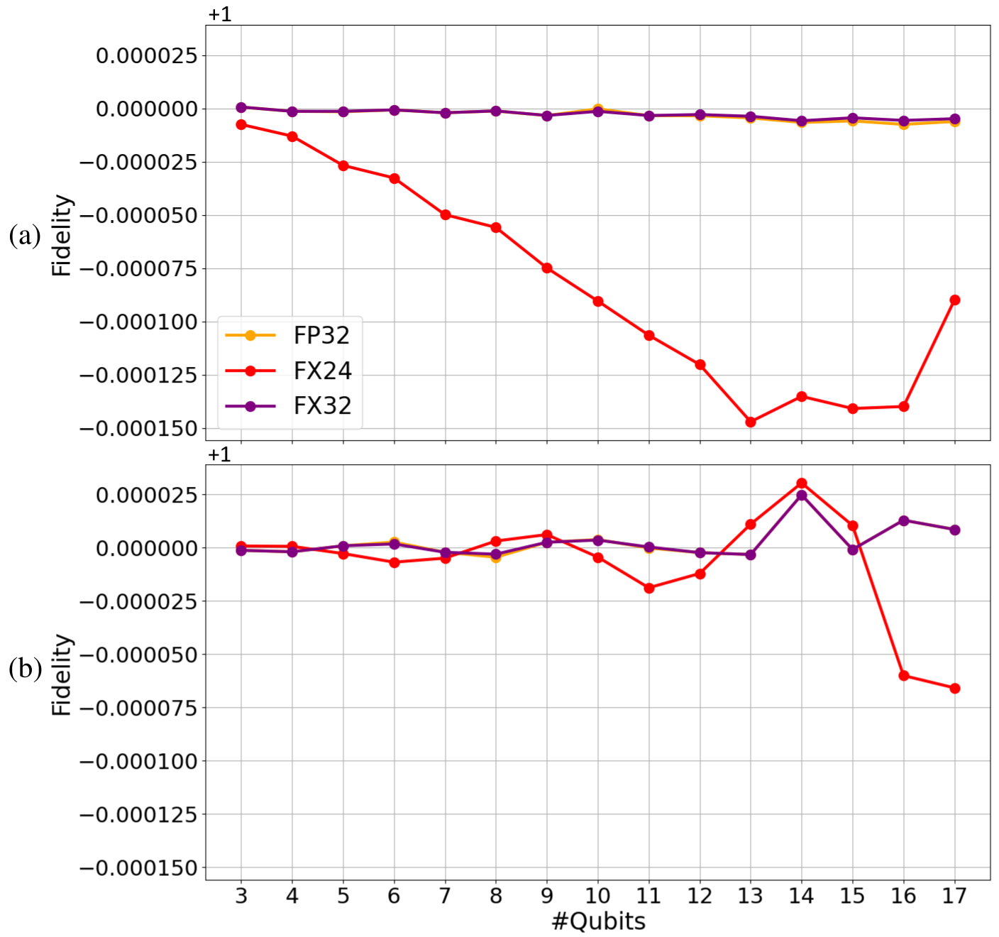
Figure 3: $\mathcal{F}_{\text{{FQsun}}^{*}}$ on performing (a) QFT and (b) PSR.

While MSE can provide a preliminary assessment of accuracy in quantum emulators, fidelity is the more precise metric for evaluating the performance of quantum simulation systems. The fidelity results for QFT and PSR, as shown in Fig. 3, demonstrate that $\mathcal{F}_{\text{{FP32}/{FX32}}(\text{QFT}/\text{PSR})}\in[0.999993,1.000024]$, have prominently small variations. Both designs exhibit stable performance, with values consistently close to $1$, indicating near-ideal accuracy. This positions FP32 and FX32 as the optimal choices in terms of fidelity. On the other hand, $\mathcal{F}_{\text{{FX24}(\text{QFT}/\text{PSR})}}\in[0.999940,1.000030]$, shows slightly larger variations. While FX24 still maintains a high level of accuracy, these more noticeable deviations suggest a lower stability compared to FP32 and FX32.

The fidelity results for RQC, presented in Fig. 4, further emphasize the accuracy gap between the three designs, particularly at $d=10$. Specifically, $\mathcal{F}_{\text{{FP32}}/\text{{FX32}}(\text{RQC})}\in[0.9999992335,1.0000001195]$, remaining measurably close to $1$. Both designs demonstrate superior stability and precision, making them the best performers among the three. By contrast, $\mathcal{F}_{\text{{FX24}}(\text{RQC})}\in[0.9999760482,0.9999979679]$ shows a broader range of fidelity values. The larger variations, especially at higher #Qubits, indicate that FX24 is less stable and slightly less accurate compared to FP32 and FX32. In summary, fidelity analysis across these applications confirms that FP32 and FX32 are the most accurate and stable designs, consistently outperforming FX24 in terms of fidelity, particularly at deeper circuit depths. Therefore, FP32 and FX32 emerge as the superior options for quantum emulation when high fidelity is critical.

To maintain the accuracy of FPGA, we list all the feasible data structures. We also evaluate the impact of data structure on the above quantum tasks. Consistency with the commentary from [17], there is a trade-off between defined high fidelity and quantization bit-width. As the small scale, the required bit-width for $\mathcal{F}\approx 1$ is low but increases fast based on $\#\text{Qubits}$ [45]. This phenomenon also comes from the normalization condition, as (2).

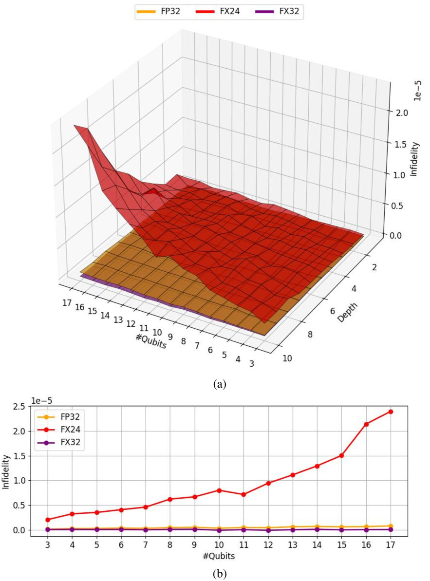
Figure 4: $(1-\mathcal{F})_{\text{{FQsun}}^{*}}$(Infidelity) on performing RQC at (a) all depth values and (b) only considering $d=10$ cases.

IV-G Detailed power consumption analysis

To accurately measure power consumption in real time, the INA226 sensor on the ZCU102 FPGA was utilized. Detailed results are shown in Fig. 5, where the power consumption values for the PS, PL, and total power are presented when FP32 version of FQsun executes RQC. Specifically, the PS consumes a maximum of $1.84$ W (with $0.34$ W dynamic power). The PL consumes a maximum of $0.61$ W. The total power reaches a maximum of $2.41$ W (with $0.23$ W dynamic power). Accordingly, the power consumption for FQsun is determined by adding the total dynamic power to the maximum PL power, reaching $0.81$ W.

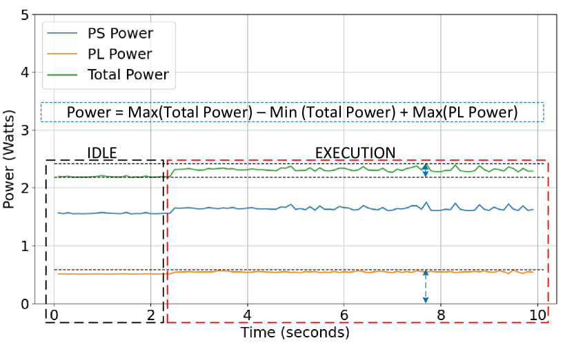
Figure 5: Power measurement of FQsun (FX32) on RQC.

IV-H Comparison with related quantum simulation on powerful CPUs and GPUs

To demonstrate the speed advantage of FQsun, the simulation time of FQsun^∗, is presented and compared with Software, running on an Intel i9-10940X CPU @ 3.30GHz.

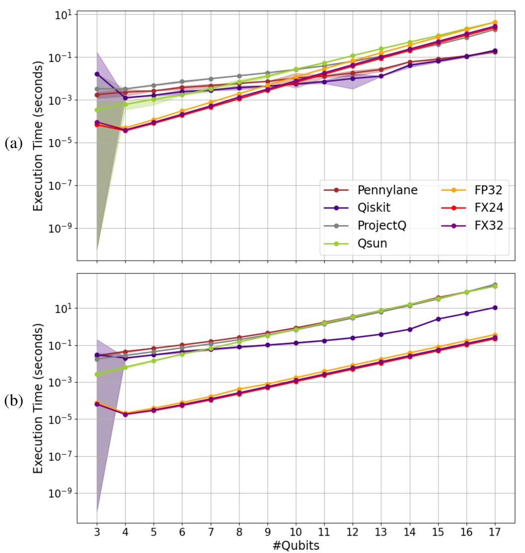
Figure 6: Mean $\pm$ standard deviation execution time of Software + $\text{{FQsun}}^{*}$ on (a) QFT and (b) PSR.

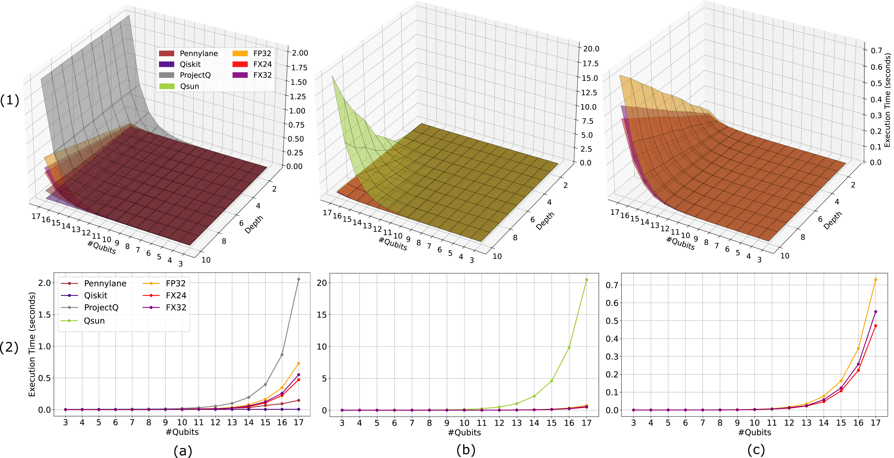
Figure 7: RQC execution time comparison between (a) Software/$\{\text{Qsun}\}$ + FQsun^∗ (b) Qsun + $\text{{FQsun}}^{*}$ and (c) $\text{{FQsun}}^{*}$. The first row (1) is the 3-D plot for vary of depth values, and the second row (2) is the case with $d=10$.

Fig. 6 shows the mean and standard deviation of the execution time of FQsun and other quantum simulators when simulating QFT and PSR. In the QFT benchmark, FQsun exhibits faster computational speed than other software simulations for $\#\text{Qubits}<10$. However, it is slower than Qiskit and PennyLane for #Qubits between 11 and 17. When executing PSR, FQsun demonstrates superior speed with significantly faster execution time compared to other software simulations.

Moreover, the comparisons in Fig. 7 include (1) FQsun^∗ with Software/{Qsun}; (2) FQsun^∗ with its software version - Qsun; and (3) among FQsun^∗ versions. Accordingly, a 2D slice at $d=10$ is also presented for better visualization. In (1), FQsun shows comparable execution speed with most software simulators at $\#\text{Qubits}<13$. The execution speed of FQsun is lower than Qiskit and PennyLane at larger depths and $\#\text{Qubits}>13$. In (2), when compared with Qsun, FQsun shows significantly faster computational speed, especially for $\#\text{Qubits}>11$, demonstrating a significant improvement over the corresponding software version. Finally, comparison (3) reveals that FQsun (FX version) provides faster computational speed, with the difference increasing gradually at $\#\text{Qubits}>13$. The execution speed decreases in the order of FQsun^∗. Overall, FQsun offers better processing speed than ProjectQ and Qsun emulators and is comparable with Qiskit and PennyLane. At the same time, the FX24 and FX32 versions are considered to have the best processing speed. Depending on the accuracy requirements, an appropriate version can be selected.

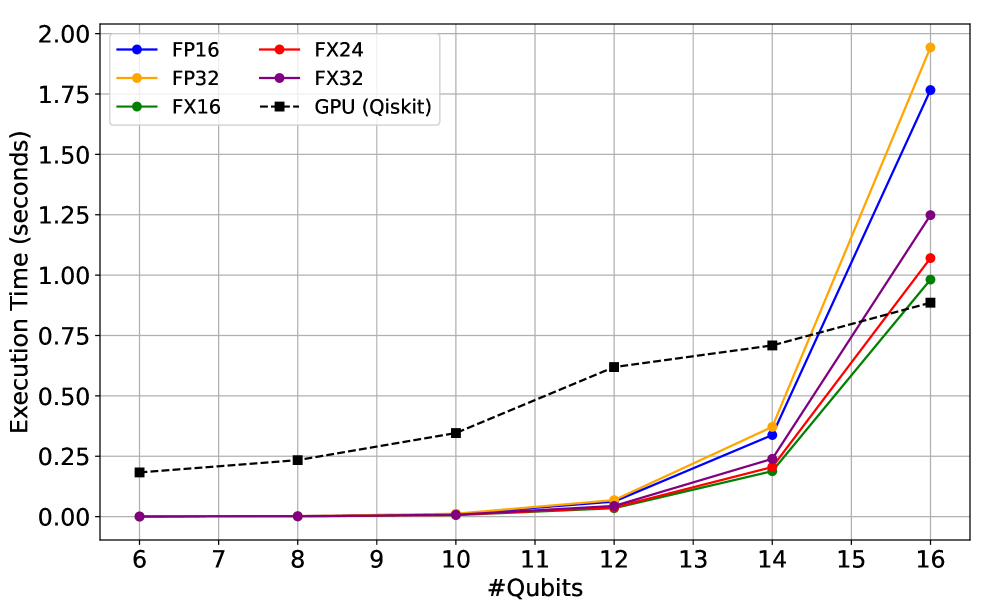
Figure 8: Estimated execution time comparison between GPU A100 [46] and FQsun on QFT.

Furthermore, Fig. 8 presents a comparison of five FQsun versions with NVIDIA A100 GPU records in the [46] database. Accordingly, QFT computation from $6$ to $16$ qubits is compared in detail. FQsun demonstrates a clear speed advantage for $\#\text{Qubits}<15$. For larger #Qubits, the GPU’s performance is slightly better due to its parallel processing nature. The highlight of FQsun is its significantly higher energy efficiency, consuming less than $1$ W of power, while GPUs typically consume hundreds.

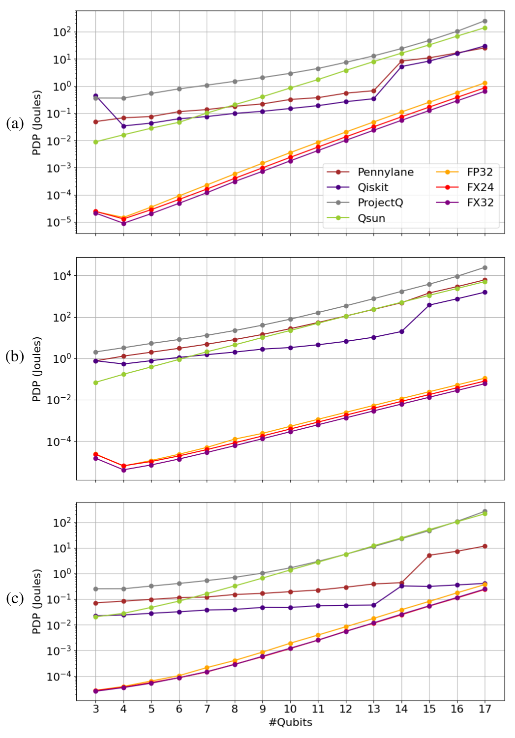
Figure 9: PDP on Software + $\text{{FQsun}}^{*}$ through (a) QFT (b) PSR and (c) RQC.

Reported work	Device	Frequency (MHz)	Precision	#Qubits	Execution time (s)	#Gates	Normalized gate speed ($\dagger$)
[17]	Xilinx XCVU9P	233	18-bit FX	16	$1.20\times 10^{-3}$	-	-
[19]	Arria 10AX115N4F45E3SG	233	32-bit FP	32	$7.92\times 10^{10}$	528	$3.49\times 10^{2}$
[20] $(\dagger\dagger)$	Xilinx XCKU115	160	16-bit FX	16	$2.70\times 10^{-1}$	136	$3.03\times 10^{-8}$
[21]	Altera Stratix EP1S80B956C6	137.9	-	3	$4.60\times 10^{-8}$	6	$9.59\times 10^{-10}$
[22]	Altera Stratix EP1S80B956C6	82.1	16-bit FX	3	$6.10\times 10^{-8}$	6	$1.26\times 10^{-9}$
[23]	Altera Stratix EP4SGX530KF4	90	24-bit FX	5	$2.19\times 10^{-7}$	15	$4.56\times 10^{-10}$
[24]	AMD Xilinx Zynq-7000	100	32-bit FX	4	$4.00\times 10^{-6}$	10	$2.50\times 10^{-8}$
[25] $(\dagger\dagger)$	Intel Stratix 10 MX2100	299	32-bit FP	30	$4.47$	465	$8.95\times 10^{-12}$
This work	Xilinx ZCU102	150	16-bit FP	18	$8.90$	810	$4.19\times 10^{-8}$
		136	32-bit FP	17	$4.30$	721	$4.55\times 10^{-8}$
		136	16-bit FX	18	$4.90$	810	$2.31\times 10^{-8}$
		125	24-bit FX	17	$2.41$	721	$2.52\times 10^{-8}$
		125	32-bit FX	17	$2.81$	721	$2.97\times 10^{-8}$

• The normalized gate speed (s / (gate $\times$ amplitude)) is calculated as the total execution time divided by the product of the #Gates and $2^{\#\text{Qubits}}$, smaller is better.

• These emulators are designed for only QFT applications.

TABLE VII: Comparative analysis of FQsun and existing FPGA-Based emulators on QFT’s performance.

To further demonstrate energy efficiency, Fig. 9 presents a comparison of PDP between three FQsun versions and four software simulations running on an Intel i9-10940X CPU. Accordingly, FQsun achieves significantly better PDP than software simulations in all three tasks. In QFT, FQsun provides a PDP from $1.30\times 10^{-5}$ to $1.31$, better than Software from $\bm{3.62\times 10^{2}}$ to $\bm{4.0\times 10^{4}}$ times; and from $4.14\times 10^{-6}$ to $8.04\times 10^{-2}$, better than Software from $\bm{3.18\times 10^{3}}$ to $\bm{7.84\times 10^{5}}$ times when simulating PSR. Finally, for RQC, FQsun achieves from $2.56\times 10^{-5}$ to $3.72\times 10^{-1}$, better than Software from $\bm{1.66\times 10^{0}}$ to $\bm{9.87\times 10^{3}}$ times.

Overall, the PDP comparison results show that FQsun has optimal energy efficiency, making it suitable for long-time and complex quantum simulations to save costs. The next section presents the comparison results of the proposed FQsun with other FPGA-based emulators to clarify the superior performance and flexibility of FQsun.

IV-I Comparison with Hardware-based quantum emulators

To demonstrate high performance, this section presents the detailed evaluation of five versions of FQsun on Xilinx ZCU102 FPGA compared to existing hardware emulators.

IV-I1 Comparison with FPGA-Based Emulators on QFT Computation

TABLE VIII: Comparative Analysis of FQsun and Existing Hardware Emulators Across Various Quantum Algorithms.

Reference	Device	Frequency(MHz)	Precision	#Qubits	Algorithm	Execution time(s)
[16]	UMC 180-nm CMOS Analog	-	-	6	GSA	$3.31\times 10^{-8}$
[19]	Arria 10 10AX115N4F45E3SG	233	32-bit FP	32	GSA	$7.92\times 10^{10}$
		137.9		3	QFT	$4.60\times 10^{-8}$
[21]	Altera Stratix EP1S80B956C6	85	16-bit FX	3	GSA	$4.60\times 10^{-8}$
					QFT	$6.10\times 10^{-8}$
[22]	Altera Stratix EP1S80B956C6	82.1	16-bit FX	3	GSA	$8.40\times 10^{-8}$
		90		5	QFT	$2.19\times 10^{-0}$
[23]	Altera Stratix EP4SGX530KF4	85	24-bit FX	7	GSA	$9.68\times 10^{-8}$
[24]	AMD Xilinx Zynq-7000	100	32-bit FP	4	QFT	$4.00\times 10^{-6}$
[26]	AMD Xilinx ZCVU9P	250	16-bit FX	6	Image Classification	$1.00\times 10^{-3}$
		136	32-bit FP	17		$4.30\times 10^{0}$
		125	24-bit FX	17		$2.41\times 10^{0}$
		125	32-bit FX	17	QFT	$2.81\times 10^{0}$
		136	32-bit FP	17		$3.68\times 10^{-1}$
		125	24-bit FX	17		$2.23\times 10^{-1}$
		125	32-bit FP	17	PSR	$2.59\times 10^{-1}$
		136	32-bit FP	17		$4.08\times 10^{-1}$
		125	24-bit FX	17		$2.63\times 10^{-1}$
This work	Xilinx ZCU102	125	32-bit FX	17	RQC	$3.06\times 10^{-1}$

Table VII presents a comparison between FQsun and existing FPGA-based quantum emulators [17, 19, 20, 21, 22, 23, 24, 25] in terms of frequency, precision, execution time, number of gates (#Gates), and normalized gate speed. Regarding execution time, compared to the Arria 10AX115N4F45E3SG [19], FP32 FQsun at 17 qubits achieves a computation speed-up of $1.84\times 10^{10}$ times (4.3 vs. $7.92\times 10^{10}$ seconds). Furthermore, compared to other quantum emulators [16, 19, 21, 23, 24, 26], FQsun supports computation with a higher #Qubits, demonstrating enhanced applicability for various applications. Specifically, FQsun supports computations across five precision types and offers different performance and accuracy. Although #Qubits in FQsun is lower compared to [19, 25], FQsun is a highly flexible emulator that can potentially support a wide range of quantum algorithms in the future. Notably, the QFT circuit executed by FQsun contains a much larger #Gates than the other emulators. Therefore, for a fair assessment, normalized gate speed is used to compare computational efficiency. Evidence shows that FX16 achieves a better-normalized gate speed than the related works, from 1.31 times ($3.03\times 10^{-8}$ vs. $2.31\times 10^{-8}$) to $1.51\times 10^{10}$ times ($3.49\times 10^{2}$ vs. $2.31\times 10^{-8}$).

IV-I2 Comparison with Hardware-Based Emulators on Various Quantum Algorithms Simulation

To provide a more comprehensive evaluation, Table. VIII details the computational results of FQsun^∗, compared to existing hardware-based emulators [16, 19, 21, 22, 23, 24, 26] when executing various quantum simulation algorithms. For the QFT algorithm, FQsun achieves execution times ranging from $0.241$ to $3.68$ (s) and supports up to $17$ qubits, significantly outperforming [21, 22, 23, 24]. While other emulators are fixed at some algorithms limited to QFT and GSA, FQsun is a general emulator with high precision. This application requires the emulator to possess both flexibility and high accuracy to meet its strict demands. This confirms that FQsun has flexibility comparable to software simulators, promising to be an ideal high-performance platform for more complex quantum simulation applications in the future.

V Conclusion

In conclusion, the FQsun demonstrates significant advancements in quantum emulators, delivering improved speed, accuracy, and energy efficiency compared to traditional software simulators and existing hardware emulators. Leveraging optimized memory architecture, a configurable QGU, and support for multiple number precisions, FQsun efficiently bridges the gap between simulation flexibility and hardware constraints. Experimental results reveal that FQsun achieves high fidelity and minimal MSE across various quantum tasks, outperforming comparable emulators on execution time and PDP. The emulator’s flexibility in supporting diverse quantum gates enables versatile applications, positioning FQsun as a reliable platform for advanced quantum simulation research. The limitations of WF are listed in Appendix V-B which is addressed in future works, targeting in support higher #Qubits and maintaining high precision.

Data availability

The codes and data used for this study are available at https://github.com/NAIST-Archlab/FQsun

Appendix

V-A Hardware-software co-design

Our proposed hardware proves that a quantum emulator can be more efficient than the same type which runs on CPU/GPU. To improve the performance of the emulator, the accelerated technique on software can be implemented on hardware, such as the accelerated PSR [47]. The Equation (9) consumes $2m$ quantum evaluation or $2m\times\#\text{Gates}$ gate evaluation, this process can be reduced half by saving $\{|\psi^{(\bm{t})}\rangle\}_{j=1}^{n_{\text{gate}}}$ at local memory. The object $|\psi^{(\bm{t})}\rangle$ is reused to calculate $|\psi^{(\bm{t})}(\bm{\theta}_{0:j})\rangle$, $|\psi^{(\bm{t})}(\bm{\theta}_{0:j}^{+\frac{\pi}{2}\bm{e}_{j}})\rangle$ and $|\psi^{(\bm{t})}(\bm{\theta}_{0:j}^{-\frac{\pi}{2}\bm{e}_{j}})\rangle$ ($\bm{\theta}^{\pm s_{k}}_{i:j}\equiv\bm{\theta}[i:j]\pm s\bm{e}_{k}$), trade-offing between execution time and memory space which suitable for small qubits cases. It will be useful if the memory space is enough, and the save/load time for $\{|\psi^{(\bm{t})}\rangle\}_{j=1}^{n_{\text{gate}}}$ is small. Further acceleration techniques such as gate-fusion [31] and realized-state representation [32] will be considered.

V-B The limitation of wave-function approach

FQsun is the type of quantum emulator that requires a small number of operations, however, the gate operation $\mathcal{W}(g)$ as Algorithm 1 and Algorithm 2 can not be parallelism. This weakness limits the execution time in necessarily high #Qubits. It can be covered if FQsun emulates QML models as Section IV-A3 where multiple wave functions need to be evaluated at the same time, each function $\mathcal{W}(g)$ can be processed at different cores and shared amplitudes located at local memory. The specific models such as Quantum Neural Network (QNN) [48] and Quantum Convolutional Neural Network (QCNN) [49] will be evaluated in future works.

As mentioned, the MM approach can cover single-quantum evaluation use cases. Despite of having millions cores, the familiar scaling behavior of an almost constant computation overhead at small system sizes, changes to an exponential scaling based on #Qubits, the same as FQsun, then, there is no difference on the large scale while FQsun consumes less much energy. This phenomenon can be explained by the bottleneck for save/load $|\psi^{(\bm{t})}\rangle$ at external memory. This challenge, in general, for quantum emulators has been analyzed in [50].

Tuan Hai Vu received the B.S. degree in software engineering and M.S. degree in computer science from the University of Information Technology, Vietnam National University, in 2021 and 2023, respectively. He is currently a Ph.D. student at the Architecture Lab at Nara Institute of Science and Technology, Japan, from 2024. His research interests include quantum simulation acceleration and quantum machine learning.

Vu Trung Duong Le received the Bachelor of Engineering degree in IC and hardware design from Vietnam National University Ho Chi Minh City (VNU-HCM)—University of Information Technology (UIT) in 2020, and the Master’s degree in information science from the Nara Institute of Science and Technology (NAIST), Japan, in 2022. He completed his Ph.D. degree in 2024 at NAIST, where he now serves as an Assistant Professor at the Computing Architecture Laboratory. His research interests include computing architecture, reconfigurable processors, and accelerator design for quantum emulators and cryptography.

Hoai Luan Pham received a bachelor’s degree in computer engineering from Vietnam National University Ho Chi Minh City—University of Information Technology (UIT), Vietnam, in 2018, and a master’s degree and Ph.D. degree in information science from the Nara Institute of Science and Technology (NAIST), Japan, in 2020 and 2022, respectively. Since October 2022, he has been with NAIST as an Assistant Professor and with UIT as a Visiting Lecture. His research interests include blockchain technology, cryptography, computer architecture, circuit design, and accelerators.

Quoc Chuong Nguyen received the B.S. degree in theoretical physics from the University of Natural Sciences, Vietnam National University, in 2018. He is currently a Ph.D. student at the State University of New York at Buffalo, the United States of America, starting in 2023. His research interests include quantum machine learning and algorithms for discrete optimization problems.

Yasuhiko NAKASHIMA received B.E., M.E., and Ph.D. degrees in Computer Engineering from Kyoto University in 1986, 1988 and 1998, respectively. He was a computer architect in the Computer and System Architecture Department, FUJITSU Limited from 1988 to 1999. From 1999 to 2005, he was an associate professor at the Graduate School of Economics, Kyoto University. Since 2006, he has been a professor at the Graduate School of Information Science, Nara Institute of Science and Technology. His research interests include computer architecture, emulation, circuit design, and accelerators. He is a fellow of IEICE, a senior member of IPSJ, and a member of IEEE CS and ACM.

References

- [1] P. W. Shor, “Polynomial-Time Algorithms for Prime Factorization and Discrete Logarithms on a Quantum Computer,” SIAM Review, vol. 41, no. 2, pp. 303–332, 1999.
- [2] L. K. Grover, “A fast quantum mechanical algorithm for database search,” in Proceedings of the twenty-eighth annual ACM symposium on Theory of computing, 1996, pp. 212–219.
- [3] Z. Zhou, Y. Du, X. Tian, and D. Tao, “QAOA-in-QAOA: Solving Large-Scale MaxCut Problems on Small Quantum Machines,” Phys. Rev. Appl., vol. 19, p. 024027, Feb 2023.
- [4] W. Guan, G. Perdue, A. Pesah, M. Schuld, K. Terashi, S. Vallecorsa, and J.-R. Vlimant, “Quantum machine learning in high energy physics,” Machine Learning: Science and Technology, vol. 2, no. 1, p. 011003, mar 2021.
- [5] S. Bravyi, A. W. Cross, J. M. Gambetta, D. Maslov, P. Rall, and T. J. Yoder, “High-threshold and low-overhead fault-tolerant quantum memory,” Nature, vol. 627, no. 8005, pp. 778–782, Mar 2024.
- [6] F. Arute and et al, “Quantum supremacy using a programmable superconducting processor,” Nature, vol. 574, no. 7779, pp. 505–510, 2019.
- [7] D. Bluvstein, S. J. Evered, A. A. Geim, S. H. Li, H. Zhou, T. Manovitz, S. Ebadi, M. Cain, M. Kalinowski, D. Hangleiter, J. P. Bonilla Ataides, N. Maskara, I. Cong, X. Gao, P. Sales Rodriguez, T. Karolyshyn, G. Semeghini, M. J. Gullans, M. Greiner, V. Vuletić, and M. D. Lukin, “Logical quantum processor based on reconfigurable atom arrays,” Nature, vol. 626, no. 7997, pp. 58–65, Feb 2024.
- [8] A. Javadi-Abhari and et al, “Quantum computing with Qiskit,” 2024.
- [9] D. S. Steiger, T. Häner, and M. Troyer, “ProjectQ: an open source software framework for quantum computing,” Quantum, vol. 2, p. 49, Jan. 2018.
- [10] S. V. Isakov, D. Kafri, O. Martin, C. V. Heidweiller, W. Mruczkiewicz, M. P. Harrigan, N. C. Rubin, R. Thomson, M. Broughton, K. Kissell et al., “Simulations of quantum circuits with approximate noise using qsim and cirq,” arXiv preprint arXiv:2111.02396, 2021.
- [11] M. Broughton, G. Verdon, T. McCourt, A. J. Martinez, J. H. Yoo, S. V. Isakov, P. Massey, R. Halavati, M. Y. Niu, A. Zlokapa, E. Peters, O. Lockwood, A. Skolik, S. Jerbi, V. Dunjko, M. Leib, M. Streif, D. V. Dollen, H. Chen, S. Cao, R. Wiersema, H.-Y. Huang, J. R. McClean, R. Babbush, S. Boixo, D. Bacon, A. K. Ho, H. Neven, and M. Mohseni, “TensorFlow Quantum: A Software Framework for Quantum Machine Learning,” 2021.
- [12] P. Date, D. Arthur, and L. Pusey-Nazzaro, “QUBO formulations for training machine learning models,” Scientific Reports, vol. 11, no. 1, p. 10029, 2021.
- [13] V. Bergholm and et al, “PennyLane: Automatic differentiation of hybrid quantum-classical computations,” 2022.
- [14] Bayraktar and et al, “cuQuantum SDK: A High-Performance Library for Accelerating Quantum Science,” in 2023 IEEE International Conference on Quantum Computing and Engineering (QCE), vol. 01, 2023, pp. 1050–1061.
- [15] Q. C. Nguyen, L. N. Tran, H. Q. Nguyen et al., “Qsun: an open-source platform towards practical quantum machine learning applications,” Machine Learning: Science and Technology, vol. 3, no. 1, p. 015034, 2022.
- [16] S. Mourya, B. R. L. Cour, and B. D. Sahoo, “Emulation of Quantum Algorithms Using CMOS Analog Circuits,” IEEE Transactions on Quantum Engineering, vol. 4, pp. 1–16, 2023.
- [17] S. Liang, Y. Lu, C. Guo, W. Luk, and P. J. Kelly, “PCQ: Parallel Compact Quantum Circuit Simulation,” in 2024 IEEE 32nd Annual International Symposium on Field-Programmable Custom Computing Machines (FCCM). Los Alamitos, CA, USA: IEEE Computer Society, may 2024, pp. 24–31.
- [18] El-Araby and et al, “Towards Complete and Scalable Emulation of Quantum Algorithms on High-Performance Reconfigurable Computers,” IEEE Transactions on Computers, vol. 72, no. 8, pp. 2350–2364, 2023.
- [19] N. Mahmud, B. Haase-Divine, A. Kuhnke et al., “Efficient Computation Techniques and Hardware Architectures for Unitary Transformations in Support of Quantum Algorithm Emulation,” Journal of Signal Processing Systems, vol. 92, pp. 1017–1037, 2020.
- [20] Y. Hong, S. Jeon, S. Park, and B.-S. Kim, “Quantum Circuit Simulator based on FPGA,” in 2022 13th International Conference on Information and Communication Technology Convergence (ICTC), 2022, pp. 1909–1911.
- [21] M. Aminian, M. Saeedi, M. S. Zamani, and M. Sedighi, “FPGA-Based Circuit Model Emulation of Quantum Algorithms,” in Proceedings of the 2008 IEEE Computer Society Annual Symposium on VLSI, ser. ISVLSI ’08. USA: IEEE Computer Society, 2008, p. 399–404.
- [22] A. Khalid, Z. Zilic, and K. Radecka, “Fpga emulation of quantum circuits,” in IEEE International Conference on Computer Design: VLSI in Computers and Processors, 2004. ICCD 2004. Proceedings., 2004, pp. 310–315.
- [23] Y. H. Lee, M. Khalil-Hani, and M. N. Marsono, “An FPGA-Based Quantum Computing Emulation Framework Based on Serial-Parallel Architecture,” International Journal of Reconfigurable Computing, vol. 2016, no. 1, p. 5718124, 2016.
- [24] A. Silva and O. G. Zabaleta, “FPGA quantum computing emulator using high level design tools,” in 2017 Eight Argentine Symposium and Conference on Embedded Systems (CASE), 2017, pp. 1–6.
- [25] H. M. Waidyasooriya, H. Oshiyama, Y. Kurebayashi, M. Hariyama, and M. Ohzeki, “A Scalable Emulator for Quantum Fourier Transform Using Multiple-FPGAs With High-Bandwidth-Memory,” IEEE Access, vol. 10, pp. 65 103–65 117, 2022.
- [26] T. Suzuki, T. Miyazaki, T. Inaritai, and T. Otsuka, “Quantum AI Simulator Using a Hybrid CPU-FPGA Approach,” 2022, last Accessed: October 2022.
- [27] C. Huang, M. Newman, and M. Szegedy, “Explicit Lower Bounds on Strong Quantum Simulation,” IEEE Transactions on Information Theory, vol. 66, no. 9, pp. 5585–5600, Sep. 2020.
- [28] J. Mei, M. Bonsangue, and A. Laarman, “Simulating quantum circuits by model counting,” in Computer Aided Verification, A. Gurfinkel and V. Ganesh, Eds. Cham: Springer Nature Switzerland, 2024, pp. 555–578.
- [29] K. Svore, A. Geller, M. Troyer, J. Azariah, C. Granade, B. Heim, V. Kliuchnikov, M. Mykhailova, A. Paz, and M. Roetteler, “Q#: Enabling Scalable Quantum Computing and Development with a High-level DSL,” in Proceedings of the Real World Domain Specific Languages Workshop 2018, ser. RWDSL2018. New York, NY, USA: Association for Computing Machinery, 2018.
- [30] S. V. Isakov and et al, “Simulations of Quantum Circuits with Approximate Noise using qsim and Cirq,” 2021.
- [31] T. Häner and D. S. Steiger, “0.5 petabyte simulation of a 45-qubit quantum circuit,” in Proceedings of the International Conference for High Performance Computing, Networking, Storage and Analysis, ser. SC ’17. New York, NY, USA: Association for Computing Machinery, 2017.
- [32] K.-S. Jin and G.-I. Cha, “QPlayer: Lightweight, scalable, and fast quantum simulator,” ETRI Journal, vol. 45, no. 2, pp. 304–317, 2023.
- [33] F. Pan, P. Zhou, S. Li, and P. Zhang, “Contracting Arbitrary Tensor Networks: General Approximate Algorithm and Applications in Graphical Models and Quantum Circuit Simulations,” Phys. Rev. Lett., vol. 125, p. 060503, Aug 2020.
- [34] S. Patra, S. S. Jahromi, S. Singh, and R. Orús, “Efficient tensor network simulation of IBM’s largest quantum processors,” Phys. Rev. Res., vol. 6, p. 013326, Mar 2024.
- [35] Y. Suzuki and et al, “Qulacs: a fast and versatile quantum circuit simulator for research purpose,” Quantum, vol. 5, p. 559, Oct. 2021.
- [36] S. Aaronson and D. Gottesman, “Improved simulation of stabilizer circuits,” Phys. Rev. A, vol. 70, p. 052328, Nov 2004.
- [37] T. Jones, A. Brown, I. Bush, and S. C. Benjamin, “QuEST and High Performance Simulation of Quantum Computers,” Scientific Reports, vol. 9, no. 1, p. 10736, Jul 2019.
- [38] M. Schuld and F. Petruccione, Machine learning with quantum computers. Springer, 2021, vol. 676.
- [39] D. Wierichs, J. Izaac, C. Wang, and C. Y.-Y. Lin, “General parameter-shift rules for quantum gradients,” Quantum, vol. 6, p. 677, Mar. 2022.
- [40] D. Wakeham and M. Schuld, “Inference, interference and invariance: How the Quantum Fourier Transform can help to learn from data,” 2024.
- [41] T. H. Vu, V. T. D. Le, H. L. Pham, and N. Yasuhiko, “Efficient Random Quantum Circuit Generator: A Benchmarking Approach for Quantum Simulators,” in 2024 RIVF International Conference on Computing and Communication Technologies (RIVF), 2024.
- [42] D. Coppersmith, “An approximate Fourier transform useful in quantum factoring,” 2002.
- [43] A. Y. Kitaev, “Quantum measurements and the Abelian Stabilizer Problem,” 1995.
- [44] P. Shor, “Algorithms for quantum computation: discrete logarithms and factoring,” in Proceedings 35th Annual Symposium on Foundations of Computer Science, 1994, pp. 124–134.
- [45] A. Laing, A. Peruzzo, A. Politi, M. R. Verde, M. Halder, T. C. Ralph, M. G. Thompson, and J. L. O’Brien, “High-fidelity operation of quantum photonic circuits,” Applied Physics Letters, vol. 97, no. 21, p. 211109, 11 2010.
- [46] A. Jamadagni, A. M. Läuchli, and C. Hempel, “Benchmarking Quantum Computer Simulation Software Packages: State Vector Simulators,” 2024.
- [47] V. T. Hai and et al., “Efficient Parameter-Shift Rule Implementation for Computing Gradient on Quantum Simulators,” in 2024 International Conference on Advanced Technologies for Communications (ATC), 2024.
- [48] M. Schuld, I. Sinayskiy, and F. Petruccione, “The quest for a quantum neural network,” Quantum Information Processing, vol. 13, pp. 2567–2586, 2014.
- [49] M. Henderson, S. Shakya, S. Pradhan, and T. Cook, “Quanvolutional neural networks: powering image recognition with quantum circuits,” Quantum Machine Intelligence, vol. 2, no. 1, p. 2, Feb 2020. [Online]. Available: https://doi.org/10.1007/s42484-020-00012-y
- [50] T. X. H. Le, H. L. Pham, T. H. Vu, V. T. D. Le, and N. Yasuhiko, “Theoretical Analysis of the Efficient-Memory Matrix Storage Method for Quantum Emulation Accelerators with Gate Fusion on FPGAs,” in 2024 IEEE 17th International Symposium on Embedded Multicore/Many-core Systems-on-Chip (MCSoC), 2024.