Decoding Quasi-Cyclic Quantum LDPC Codes

Abstract

Quantum low-density parity-check (qLDPC) codes are an important component in the quest for quantum fault tolerance. Dramatic recent progress on qLDPC codes has led to constructions which are asymptotically good, and which admit linear-time decoders to correct errors affecting a constant fraction of codeword qubits [PK22a, LZ23, DHLV23, GPT23]. These constructions, while theoretically explicit, rely on inner codes with strong properties only shown to exist by probabilistic arguments, resulting in lengths that are too large to be practically relevant. In practice, the surface/toric codes, which are the product of two repetition codes, are still often the qLDPC codes of choice.

A construction preceding [PK22a] based on the lifted product of an expander-based classical LDPC code with a repetition code [PK22b] achieved a near-linear distance (of $\Omega(N/\log N)$ where $N$ is the number of codeword qubits), and avoids the need for such intractable inner codes. Our main result is an efficient decoding algorithm for these codes that corrects $\Theta(N/\log N)$ adversarial errors. En route, we give such an algorithm for the hypergraph product version these codes, which have weaker $\Theta(\sqrt{N})$ distance (but are simpler). Our decoding algorithms leverage the fact that the codes we consider are quasi-cyclic, meaning that they respect a cyclic group symmetry.

Since the repetition code is not based on expanders, previous approaches to decoding expander-based qLDPC codes, which typically worked by greedily flipping code bits to reduce some potential function, do not apply in our setting. Instead, we reduce our decoding problem (in a black-box manner) to that of decoding classical expander-based LDPC codes under noisy parity-check syndromes. For completeness, we also include a treatment of such classical noisy-syndrome decoding that is sufficient for our application to the quantum setting.

1 Introduction

Quantum low-density parity-check (qLDPC) codes provide a particularly promising avenue for achieving low-overhead quantum error correction. Alongside code design, one of the most important challenges associated with qLDPC codes is the design of efficient decoding algorithms, which are needed to correct errors more quickly than they occur in quantum devices. In this paper, we present new efficient algorithms to decode qLDPC codes arising from a product of a classical LDPC code and a repetition code against a number of adversarial errors growing linearly in the code distance. As described below, the problem of decoding such quantum codes arise in various settings of interest, and even permits a purely classical interpretation. To the best of our knowledge, our results provide the first known polynomial-time decoding algorithms for these codes.

A qLDPC code is a quantum code for which errors on code states can be corrected by first performing some constant-weight quantum stabilizer (i.e. parity-check) measurements, and then running a classical decoding procedure that processes these measurement outcomes to identify an appropriate correction that will revert the effect of the error. The stabilizer measurements are typically efficient, at least in theory, as they by definition each only involve a constant number of qubits. Therefore a key challenge in decoding qLDPC codes is to define a classical decoding algorithm, which receives as input the stabilizer measurement outcomes, called the syndrome. This algorithm must output a Pauli correction that can be applied to revert the effect of the physical error on the code qubits.

We typically want to design efficient decoding algorithms for qLDPC codes with large distance and dimension relative to the length, or number of physical qubits. The distance of a code measures the maximum number of corruptions from which the original code state can be recovered information-theoretically (but possibly inefficiently). In particular, codes of distance $D$ permit information-theoretic error-correction from adversarial errors acting on up to $(D-1)/2$ physical code qubits. Meanwhile, the dimension of a code equals the number of logical qubits that can be encoded in the code.

For over two decades, there were no known qLDPC codes of length $N$ and distance above $\tilde{O}(\sqrt{N})$, which up to poly-logarithmic factors is the distance achieved by Kitaev’s Toric code [Kit03]. However, a recent breakthrough line of work achieved the first qLDPC codes of distance $N^{1/2+\Omega(1)}$ [HHO21, BE21, Has23], culminating first in qLDPC codes of nearly linear distance $D=\Theta(N/\log N)$ with dimension $K=\Theta(\log N)$ [PK22b], and then finally of linear distance $D=\Theta(N)$ and dimension $K=\Theta(N)$ (i.e. asymptotically good) [PK22a]. The construction of [PK22a], along with some spinoff constructions [LZ22, DHLV23], remain the only known linear-distance qLDPC codes. Meanwhile, the codes of [PK22b] remain the only other known construction of qLDPC codes with almost linear distance $D\geq N^{1-o(1)}$.

The codes of [PK22a, LZ22, DHLV23], though asymptotically good in theory, are constructed using inner codes for which the only known constructions are randomized and prohibitively large in practice. In contrast, the nearly-linear-distance codes of [PK22b] are constructed as a product of an expander-based classical LDPC code with a repetition code, and thereby avoid the need for such intractable inner code properties. These codes of [PK22b] are said to be quasi-cyclic, as they respect the action of a large cyclic group, in part due to the cyclic symmetry of the repetition code.

The asymptotically good codes of [PK22a, LZ22, DHLV23] have been shown to have linear-time decoders [GPT23, LZ23, DHLV23], which can be parallelized to run in logarithmic time [LZ23]. However, to the best of our knowledge, there were no known polynomial-time decoding algorithms for the nearly-linear distance quasi-cyclic codes of [PK22b]. Such a decoder is our principal contribution:

Theorem 1 (Informal statement of Theorem 32 with Proposition 24).

There exists an explicit family of qLDPC codes $\mathcal{C}$ of length $N\rightarrow\infty$, dimension $K=\Theta(\log N)$, and distance $D=\Theta(N/\log N)$ obtained by instantiating the construction of [PK22b], such that the following holds. Fix any constants $0<\epsilon\leq 1/2$ and $\epsilon^{\prime}>0$. Then there is a $O(N^{2+O(\epsilon+\epsilon^{\prime})})$-time randomized decoding algorithm for $\mathcal{C}$ that successfully decodes against $\Theta(\epsilon D)$ adversarial errors with probability $\geq 1-2^{-N^{\epsilon^{\prime}}}$.

In words, Theorem 1 provides a close-to-quadratic time randomized algorithm that decodes the codes of [PK22b] from a linear number of errors with respect to the code distance, with just an exponentially small probability of a decoding failure. At a very high level, our algorithm works by making appropriate black-box calls to a classical LDPC code decoder that can handle errors on both code bits and parity-check bits.

We emphasize that Theorem 1 provides a decoding algorithm that corrects against arbitrary adversarial errors, not simply randomized errors. The randomization and exponentially small failure probability in Theorem 1 instead arise from a randomized component of the decoding algorithm. As shown in Section 6, we depress the failure probability to be exponentially small using standard amplification techniques; we can similarly detect decoding failures when they do occur.

1.1 Overview of QLDPC Code Constructions

The nearly linear-distance quasi-cyclic qLDPC codes of [PK22b] in Theorem 1 are constructed as the lifted product (see Section 2.7) of a classical Tanner code (on an expander graph) with a repetition code. Lifted products provide a general means for constructing a quantum code from two classical codes that respect a group symmetry.

The asymptotically good qLDPC codes of [PK22a, LZ22, DHLV23] are also constructed using a lifted product, but of two classical Tanner codes on expander graphs (see also [TZ14]). Meanwhile, the Toric code [Kit03] is constructed as a product of two repetition codes. We remark that the Toric code, along with the closely related surface code [BK98], has dimension $K=\Theta(1)$, distance $\Theta(\sqrt{N})$, was essentially the state-of-the-art qLDPC code for many years, and remains integral to practical quantum error correction efforts.

To summarize, many qLDPC codes of interest in the literature are constructed either as a product of two expander-based classical LDPC codes, or as a product of two repetition codes. The quasi-cyclic codes of [PK22b] interpolate between these two constructions by taking a product of an expander-based classical LDPC code with a repetition code.

Our work initiates the study of efficiently decoding such products of an expander-based code with a repetition code. Our techniques are applicable beyond the decoder in Theorem 1 for the codes of [PK22b]. For instance, we show that a similar, but less involved, decoding algorithm applies to another class of quasi-cyclic codes, obtained as a related (but different) product, namely the hypergraph product, of an expander-based classical LDPC code with a repetition code (see Section 5). The reader is referred to Section 1.3 for comparisons to prior decoders for related codes.

Such hypergraph products of expander-based codes with repetition codes arise naturally in various settings. For instance, similar such codes are used to teleport logical qubits between a product of two expander-based codes and a surface code; see for instance [XAP⁺23].

Perhaps more fundamentally, the hypergraph product of some code $\mathcal{A}$ with a repetition code $\mathcal{B}$ can be viewed as a description of how the code $\mathcal{A}$ handles errors occuring on different code components at different points in time. At a high level, here the code $\mathcal{A}$ describes the available storage space, while the repetition code $\mathcal{B}$ serves as the time axis. This viewpoint is often used in quantum error correction to design decoding algorithms, such as for the surface code, that are robust against syndrome errors (see e.g. [DKLP02]). Appendix A applies this viewpoint to give a fully classical interpretation of our decoding algorithm for quantum hypergraph product codes.

1.2 Overview of Decoding Techniques

Our decoding algorithm for the codes $\mathcal{C}$ in Theorem 1 leverages the group symmetry that $\mathcal{C}$ respects due to its quasi-cyclic nature. If we arrange the bits of a length-$\ell$ repetition code in a circle, then the code is preserved under the cyclic group action of $\mathbb{Z}/\ell\mathbb{Z}$, where $i\in\mathbb{Z}/\ell\mathbb{Z}$ simply shifts all bits by $i$ positions clockwise. As $\mathcal{C}$ is obtained as a product of an expander-based code (also respecting a cyclic group action) with a length-$\ell$ repetition code, $\mathcal{C}$ inherits this action of $\mathbb{Z}/\ell\mathbb{Z}$. Therefore the code space of $\mathcal{C}$ is preserved under permutations of the qubits by actions of the group $\mathbb{Z}/\ell\mathbb{Z}$, so $\mathcal{C}$ is indeed a quasi-cyclic quantum code.

At a high level, our decoder in Theorem 1 repeatedly adds together different cyclic shifts of the received syndrome, and then passes this sum through a classical Tanner code decoder to gain information about the original error. Our algorithm can use, in a black-box manner, any such classical decoder that corrects against errors on the code bits in the presence of errors on the parity-check syndrome bits. The main idea is that we isolate the effects of certain errors by summing together different cyclic shifts of the syndrome; we can then identify, and ultimately correct, these errors. [PK22b] used a related idea to prove the distance bound in these codes.

However, our actual algorithm is rather delicate, and requires an iterative aspect that is absent from the distance proof of [PK22b]. Specifically, our algorithm consists of $\Theta(\log\ell)$ iterations, where the $\tau$th iteration adds together $2^{\tau}$ cyclic shifts of the syndrome, and uses a classical Tanner code decoder to perform some analysis with a constant probability of failure. With probability $2^{-\Theta(\log\ell)}=1/\operatorname{poly}(\ell)$, all iterations succeed, and we decode successfully. We then amplify the success probability by repeating this procedure $\operatorname{poly}(\ell)$ times.

1.3 Comparison to Prior Decoders

Our techniques described above differ from those used in decoders of [GPT23, LZ23, DHLV23] for asymptotically good qLDPC codes [PK22a, LZ22, DHLV23]. At a high level, given a syndrome, these decoders recover the error by greedily flipping code bits to reduce some potential function related to the syndrome weight. Such greedy “flip”-style decoders are often applied for expander-based classical and quantum LDPC codes (e.g. [SS96, Zem01, LTZ15, FGL18]). However, beacuse the quasi-cyclic codes of [PK22b] that we consider in Theorem 1 are constructed with products involving repetition codes, which are not based on expanders, the resulting codes $\mathcal{C}$ do not seem to be “sufficiently expanding” to permit such a greedy flip-style decoder.

All previously known decoders [GPT23, LZ23, DHLV23] for linear (or almost linear) distance qLDPC codes [PK22a, LZ22, DHLV23] require the code to be constructed from a constant-sized pair of “inner codes” satisfying a property called (two-way) product-expansion (also known as robust testability; see e.g. [KP23, DHLV23]). Such constant-sized objects have been shown to exist via probabilistic arguments. However, the constants are prohibitively large to the point where no specific instances of such two-way product-expanding codes have been constructed, to the best of our knowledge.

In contrast, the codes of [PK22b] do not need product-expanding inner codes, and hence may be more relevant for practical implementations. Furthermore, as mentioned in Section 1.2, our decoding algorithm in Theorem 1 is based on the black-box application of classical LDPC code decoders in the quantum setting, which may be helpful for implementation purposes. In contrast, the flip-style decoders of [GPT23, LZ23, DHLV23] are more inherently quantum, as they do not naturally reduce to decoding a good classical code.

For hypergraph products of arbitrary classical codes, the ReShape decoder of [QC22] can also correct a linear number adversarial errors with respect to the code distance, and also is based on a black-box application of classical decoders. While we restrict attention to products of expander-based codes with repetition codes, we are able to decode lifted products of nearly linear distance, whereas [QC22] only consider hypergraph products (which have distance at most $O(\sqrt{N})$ for codes of length $N$). Furthermore, for hypergraph products, we present a decoding algorithm that runs in almost linear time with respect to the block length (see Section 3.1), whereas ReShape requires quadratic running time [QC22].

One downside of the codes of [PK22b] that we consider is their logarithmic dimension $K=\Theta(\log N)$, which is much worse than the optimal $K=\Theta(N)$. We can boost the dimension at the cost of degrading the distance by simply breaking the message into equal-sized blocks, and encoding each block into a smaller instance of the codes of [PK22b]. Indeed, for any $0<\alpha<1$, we can obtain length-$N$ qLDPC codes of dimension $K=\Theta(N^{\alpha}\log N)$ and distance $D=\Theta(N^{1-\alpha}/\log N)$ by simply using $N^{\alpha}$ copies of the length-$N^{1-\alpha}$ code of [PK22b]. Our decoder in Theorem 1 by definition still applies to such codes. [PK22b] showed how to improve these parameters to $K=\Theta(N^{\alpha}\log N)$ and $D=\Theta(N^{1-\alpha/2}/\log N)$ using an additional product construction, though we have not analyzed the decoding problem for these codes. It is an interesting question whether the dimension of such constructions could be further increased, while preserving the distance and efficient decodability, and without requiring a stronger ingredient such as product-expansion.

1.4 Open Problems

Our work raises a number of open problems, such as those listed below:

• Can our decoding algorithms be adapted to correct a number of random errors growing linearly in the block length?

• Can our decoding algorithms be made to accomodate syndrome measurement errors? Note that our algorithms use as an ingredient classical codes robust to syndrome errors, which is distinct from considering errors on the syndrome of the quantum code.

• Can our decoding algorithms be parallelized? We see no impediment to parallelization, but for simplicity in the presentation we did not pursue this direction.

• Can our techniques be used to improve decoder performance in practical implementations? Our black-box use of classical LDPC decoders may be useful in this regard.

• Can our techniques be extended to more general classes of codes, or to codes with improved paramters? See for instance the discussion in Section 1.3.

1.5 Roadmap

The remainder of this paper is organized as follows. Section 2 provides necessary preliminary notions on classical and quantum codes. For completeness Section 2 is fairly detailed, but readers familiar with quantum LDPC codes and the language of chain complexes may skip most of this background and head directly to Section 3, which provides a technical overview of our decoding algorithms. Section 4 describes the classical LDPC codes that we use in a black-box manner for the quantum codes we consider. Section 5 presents our decoder for the hypergraph product of an expander-based classical LDPC code with a repetition code. This hypergraph product decoder provides a helpful introduction to some of the basic techniques involved in the proof of our main result (Theorem 1) on decoding lifted products of such classical codes. We prove Theorem 1 in Section 6.

Appendix A provides a purely classical interpretation of our hypergraph product decoder. This perspective may be particularly helpful for those more familiar with classical error correction.

Appendix B provides the formal construction of the expander-based classical LDPC codes we describe in Section 4, and proves the necessary properties. In particular, Appendix B provides a self-contained presentation of efficient decoding of classical LDPC codes, along with their “transpose” codes, under errors on both the code bits and syndrome bits.

2 Preliminaries

This section presents preliminary notions and relevant prior results pertaining to classical and quantum codes. For simplicity, in this paper we restrct attention to codes over the binary alphabet $\mathbb{F}_{2}$.

2.1 Basic Notation

For an integer $n\geq 0$, we let $[n]=\{0,\dots,n-1\}$ denote the set of nonnegative integers less than $n$.

2.2 Chain Complexes

It will be most convenient for us to phrase both classical and quantum codes in the (standard) language of chain complexes.

Definition 2.

A $t$-term chain complex (over $\mathbb{F}_{2}$) $\mathcal{C}_{*}$ consists of an $\mathbb{F}_{2}$-vector space $C_{*}=\bigoplus_{i\in[t]}C_{i}$ where each $C_{i}$ is an $\mathbb{F}_{2}$-vector space, along with a linear boundary map $\partial:C_{*}\rightarrow C_{*}$ satisfying $\partial^{2}=0$ and $\partial(C_{i})\subseteq C_{i-1}$. Letting $\partial_{i}=\partial|_{C_{i}}$, we summarize the components of the chain complex by writing

$$\mathcal{C}_{*}=\left(C_{t-1}\xrightarrow{\partial_{t-1}}C_{t-2}\xrightarrow{\partial_{t-2}}\cdots\xrightarrow{\partial_{1}}C_{0}\right).$$

In this paper we asume all $C_{i}$ are finite-dimensional. Then $C_{*}$ has an associated dual chain complex $\mathcal{C}^{*}=(C^{*},\delta)$, called the cochain complex, given by

$$\mathcal{C}^{*}=\left(C^{t-1}\xleftarrow{\delta_{t-2}}C^{t-2}\xleftarrow{\delta_{t-3}}\cdots\xleftarrow{\delta_{0}}C^{0}\right),$$

where each $C^{i}=C_{i}$, so that $C^{*}=C_{*}$, and $\delta_{i}=\partial_{i+1}^{\top}$, so that $\delta=\partial^{\top}$. The boundary map $\delta$ of $\mathcal{C}^{*}$ is called the coboundary map of $\mathcal{C}_{*}$.

For each $i\in[t]$, we furthermore let

$$Z_{i}(\mathcal{C}) =\ker\partial_{i}\hskip 10.00002pt\text{ be the space of {$i$-cycles}},$$

$$B_{i}(\mathcal{C}) =\operatorname{im}\partial_{i+1}\hskip 10.00002pt\text{ be the space of {$i$-boundaries}},$$

$$H_{i}(\mathcal{C}) =Z_{i}(\mathcal{C})/B_{i}(\mathcal{C})\hskip 10.00002pt\text{ be the {$i$-homology group}},$$

where we let $\partial_{i}=0$ for all $i\notin\{1,\dots,t-1\}$. The $i$-cocycles $Z^{i}(\mathcal{C})$, $i$-coboundaries $B^{i}(\mathcal{C})$, and $i$-cohomology group $H^{i}(\mathcal{C})$ are defined analogously for the cochain complex.

Sometimes for clarity we will denote the boundary map of $\mathcal{C}_{*}$ by $\partial^{\mathcal{C}}=\partial$, and similarly denote the coboundary map $\delta^{\mathcal{C}}=\delta$.

We say that the chain complex $\mathcal{C}_{*}$ is based if each $C_{i}$ has some fixed basis.

For the purpose of this paper, we assume all of our chain complexes are based, and often write “chain complex” to implicitly mean “based chain complex.” The based condition gives a well-defined notion of Hamming weight:

Definition 3.

Let $C$ be a finite-dimension $\mathbb{F}_{2}$-vector space with a fixed basis, so that every $c\in C$ can be expressed as $c=(c_{0},\dots,c_{n-1})$ where $n=\dim C$ and each $c_{i}\in\mathbb{F}_{2}$. Then the Hamming weight of $c$ is

$$|c|=|\{i\in[n]:c_{i}\neq 0\}|.$$

We extend this definition to sets $S\subseteq C$ (where $S$ may not be a linear subspace) by defining

$$|S|=\min_{c\in S}|c|.$$

2.3 Classical and Quantum Codes as Chain Complexes

In this section, we present standard definitions of classical and quantum codes. However, we treat these codes using the language of chain complexes, which is standard in the quantum coding literature, but perhaps not in the classical literature.

Definition 4.

A classical linear code (or simply classical code) of block length $n$ is a subspace $C\subseteq\mathbb{F}_{2}^{n}$. The dimension $k$ of $C$ is its dimension as an $\mathbb{F}_{2}$-vector space, that is, $k=\dim_{\mathbb{F}_{2}}C$. The distance $d$ of $C$ is the minimum Hamming weight of a nonzero vector in $C$, that is, $d=\min_{c\in C\setminus\{0\}}|c|$. If $C$ has block length $n$, dimension $k$, and distance $\geq d$, we say that $C$ is an $[n,k,d]$ code. The dual of $C$ is the $(n-k)$-dimensional code $C^{\perp}=\{c^{\prime}\in\mathbb{F}_{2}^{n}:c^{\prime}\cdot c=0\;\forall c\in C\}$.

It will often be helpful to treat classical codes in the language of chain complexes, as described below.

Definition 5.

Every 2-term chain complex $\mathcal{C}_{*}=(C_{1}\xrightarrow{\partial_{1}}C_{0})$ has an associated classical code $\ker\partial_{1}\subseteq C_{1}$. The operator $\partial_{1}:C_{1}\rightarrow C_{0}$ is called a parity-check matrix of the code $\ker\partial_{1}$.

We now define quantum CSS codes:

Definition 6.

A quantum CSS code (or simply quantum code) of block length $n$ is a pair $C=(C_{X},C_{Z})$ of subspaces $C_{X},C_{Z}\subseteq\mathbb{F}_{2}^{n}$ such that $C_{Z}^{\perp}\subseteq C_{X}$ (and therefore also $C_{X}^{\perp}\subseteq C_{Z}$). The dimension $k$ of $C$ is given by

$$k=\dim(C_{Z})-\dim(C_{X}^{\perp})=\dim(C_{X})-\dim(C_{Z}^{\perp}),$$

and the distance $d$ of $C$ is given by

$$d=\min_{c\in(C_{Z}\setminus C_{X}^{\perp})\cup(C_{X}\setminus C_{Z}^{\perp})}|c|.$$

If $C$ has block length $n$, dimension $k$, and distance $\geq d$, we say that $C$ is an $[[n,k,d]]$ code.

Just as a classical code can be obtained from a 2-term chain complex, a quantum code can similarly be obtained from a 3-term chain complex:

Definition 7.

Every 3-term chain complex $\mathcal{C}_{*}=(C_{2}\xrightarrow{\partial_{2}}C_{1}\xrightarrow{\partial_{1}}C_{0})$ has an associated quantum code $C=(C_{X}=\ker\delta_{1},C_{Z}=\ker\partial_{1})$, where we recall that $\delta_{1}=\partial_{2}^{\top}$. The operators $\delta_{1}$ and $\partial_{1}$ are called X and Z parity-check matrices, respectively.

For a 3-term chain complex $\mathcal{C}_{*}$, the condition that $\partial_{1}\partial_{2}=0$ is equivalent to the condition that the associated CSS code $(C_{X},C_{Z})$ satisfies $C_{X}^{\perp}\subseteq C_{Z}$. Thus chain complexes indeed are a natural language for describing CSS codes.

By definition, the quantum code associated to a 3-term chain complex $\mathcal{C}_{*}$ has dimension

$$k=\dim H_{1}(\mathcal{C})=\dim H^{1}(\mathcal{C}),$$

and has distance

$$d=\min_{c\in(Z_{1}(\mathcal{C})\setminus B_{1}(\mathcal{C}))\cup(Z^{1}(\mathcal{C})\setminus B^{1}(\mathcal{C}))}|c|.$$

When clear from context, we will sometimes refer to a 2-term chain complex and its associated classical code interchangeably, and we will similarly refer to a 3-term chain complex and its associated quantum code interchangeably.

In this paper we are specifically interested in LDPC codes, which have sparse parity-check matrices, as defined below.

Definition 8.

The locality of a chain complex $\mathcal{C}_{*}$ is the maximum Hamming weight of any row or column of any boundary map $\partial_{i}$ in the complex.

In particular, we say that a family of complexes with locality $\leq w$ is LDPC (low-density parity-check) with locality $w$. If $w=O(1)$ is a constant, we simply say the family is LDPC.

Thus a family of 2-term chain complexes with sparse boundary maps corresponds to a family of classical LDPC codes, while a family of 3-term chain complexes with sparse boundary maps corresponds to a family of quantum LDPC codes.

2.4 Expansion and Decoding of Classical Codes

We now define some relevant notions of expansion and decoding for classical codes, or rather, for 2-term chain complexes. From this point on the reader may think of most (classical as well as quantum) codes we discuss as being LDPC unless explicitly stated otherwise, though we will only formally impose the LDPC condition when necessary or useful.

To begin, we define expansion for classical codes.

Definition 9.

Let $\mathcal{C}_{*}=(C_{1}\xrightarrow{\partial_{1}}C_{0})$ be a 2-term chain complex with $N_{i}=\dim C_{i}$. Then $\mathcal{C}$ has $(\alpha,\beta)$-expansion if for every $c\in C_{1}$ such that $0<|c|\leq\alpha N_{1}$, it holds that $|\partial_{1}c|\geq\beta|c|$.

Remark 10.

Perhaps more descriptive term than expansion would be small-set expansion. There is also a generalization to chain complexes with more terms called small-set (co)boundary expansion, which turns out to be important in applications of quantum LDPC codes [HL22, ABN23]. However, we will not need this notion of small-set (co)boundary expansion for our work.

Known constructions of classical LDPC codes (e.g. [SS96]) have $(\Omega(1),\Omega(1))$-expansion for both the associated chain complex $\mathcal{C}_{*}$ and its cochain complex $\mathcal{C}^{*}$ (see Lemma 46 below).

Many of these expanding classical codes have the additional property that they can be approximately decoded from noisy syndromes, as defined below.

Definition 11.

Let $\mathcal{C}_{*}=(C_{1}\xrightarrow{\partial_{1}}C_{0})$ be a 2-term chain complex with $N_{i}=\dim C_{i}$. We say that (the code associated to) $\mathcal{C}_{*}$ is $(e_{0},e_{1},\gamma)$-noisy-syndrome decodable in time $T$ if there exists a decoding algorithm $D:C_{0}\rightarrow C_{1}$ (specifying a possibly nonlinear function) that runs in time $T$ such that for every code error $c_{1}\in C_{1}$ of weight $|c_{1}|\leq e_{1}$ and every syndrome error $c_{0}\in C_{0}$ of weight $|c_{0}|\leq e_{0}$, it holds that

$$|D(c_{0}+\partial_{1}c_{1})-c_{1}|\leq\gamma|c_{0}|.$$

In words, noisy-syndrome decodability says that given code error $c_{1}$ and syndrome error $c_{0}$, a decoder receiving the noisy syndrome $c_{0}+\partial c_{1}$ is able to approximately recover the code error, up to a loss that is at most proportional to the weight of the syndrome error $c_{0}$. Note that this loss is bounded independently of the size of the code error $c_{1}$, as long as $|c_{1}|\leq e_{1}$. For instance, in the special case of a noiseless syndrome $c_{0}=0$, whenever $|c_{1}|\leq e_{1}$ the decoder exactly recovers $c_{1}$.

This notion of noisy-syndrome decodability is really a property of the chain complex $\mathcal{C}_{*}$ rather than of the code $\ker\partial_{1}$. Indeed, the definition is meaningful even when $\ker\partial_{1}=\{0\}$, and we will use the definition for such chain complexes.

Remark 12.

Many asymptotically good $[N,\Theta(N),\Theta(N)]$ classical LDPC codes in the literature that are based on expander graphs (e.g. those in [SS96]) are $(\Theta(N),\Theta(N),\Theta(1))$-noisy-syndrome decodable in $O(N)$ time. Such a result on noisy-syndrome decoding is for instance shown in [Spi96]. However, for our purposes, we will need $\mathcal{C}$ for which both the chain complex $\mathcal{C}_{*}$ and its cochain complex $\mathcal{C}^{*}$ are noisy-syndrome decodable in linear time. We could not find such a result written in the literature, so we prove the existence of classical LDPC codes $\mathcal{C}$ with such noisy-syndrome decoders in Proposition 24.

Decoding from noisy syndromes in the quantum setting is often referred to as single-shot decoding [Bom15] (see also e.g. [Cam19, FGL20, KV22, GTC⁺23]). In this paper, we use classical noisy-syndrome decoding to construct decoders for quantum codes, but we do not consider noisy syndromes of the quantum codes themselves. It is an interesting question to determine if our techniques extend to this setting.

2.5 Decoding of Quantum Codes

We now define the decoding problem for quantum codes. Unlike the classical treatment in Section 2.4, for quantum decoding we assume the decoder has access to an exact noise-free error syndrome. It is an interesting direction for future work to extend our results to allow for noisy syndromes in the quantum codes.

Definition 13.

Let $\mathcal{C}_{*}=(C_{2}\xrightarrow{\partial_{2}}C_{1}\xrightarrow{\partial_{1}}C_{0})$ be a 3-term chain complex. A decoder against $e$ (adversarial) errors for the quantum code associated to $\mathcal{C}_{*}$ is a pair of algorithms $D_{0}:C_{0}\rightarrow C_{1}$ and $D^{2}:C^{2}\rightarrow C^{1}$ (specifying possibly nonlinear functions) with the following properties:

1. For every $c\in C_{1}$ with $|c|\leq e$, it holds that $D_{0}(\partial_{1}c)\in c+B_{1}(\mathcal{C})$.

2. For every $c\in C^{1}$ with $|c|\leq e$, it holds that $D^{2}(\delta_{1}c)\in c+B^{1}(\mathcal{C})$.

If $D_{0},D^{2}$ are randomized algorithms and the above statements hold (for every $c$) with probability $\geq 1-\epsilon$ over the decoder’s randomness, we say that the decoder is randomized with failure probability $\epsilon$.

The running time of the decoder for $\mathcal{C}_{*}$ is simply the sum of the running times of $D_{0}$ and $D^{2}$.

In words, Definition 13 says that a decoder for a CSS code simply consists of an $X$ and a $Z$ decoder, each of which is given access to a sufficiently low-weight $X$ or $Z$ error syndrome respectively, and must recover the original error up to (physically irrelevant) added stabilizers.

We are interested in finding decoders that decode against a close-to-optimal number of errors. The optimal number of adversarial errors that can be corrected is one less than half the code’s distance, so we typically want decoders protecting against a linear number of errors with respect to the distance.

2.6 Hypergraph Product

This section describes how the hypergraph (i.e. homological) product of two 2-term chain complexes representing classical codes yields a 3-term chain complex representing a quantum code. This construction and its distance analysis was given in [TZ14].

Definition 14.

Let $\mathcal{A}_{*}=(A_{1}\xrightarrow{\partial^{\mathcal{A}}}A_{0})$ and $\mathcal{B}_{*}=(B_{1}\xrightarrow{\partial^{\mathcal{B}}}B_{0})$ be 2-term chain complexes. Then the hypergraph product $(\mathcal{A}\otimes_{\mathbb{F}_{2}}\mathcal{B})_{*}$ is the 3-term chain complex

$$A_{1}\otimes B_{1}\xrightarrow{\partial^{\mathcal{A}}\otimes I+I\otimes\partial^{\mathcal{B}}}A_{0}\otimes B_{1}\oplus A_{1}\otimes B_{0}\xrightarrow{I\otimes\partial^{\mathcal{B}}+\partial^{\mathcal{A}}\otimes I}A_{0}\otimes B_{0}.$$

All tensor products above are taken over $\mathbb{F}_{2}$, so we often omit the $\mathbb{F}_{2}$ subscript and for instance write $\mathcal{A}\otimes\mathcal{B}$.

The following formula for the dimension of a hypergraph product code was shown in [TZ14], and also follows from the well-known Künneth formula (see e.g. [Hat01]).

Proposition 15 (Künneth formula).

For 2-term chain complexes $\mathcal{A}_{*}$ and $\mathcal{B}_{*}$, it holds that

$$\dim H_{1}(\mathcal{A}\otimes\mathcal{B})=\dim(H_{1}(\mathcal{A}))\cdot\dim(H_{0}(\mathcal{B}))+\dim(H_{0}(\mathcal{A}))\cdot\dim(H_{1}(\mathcal{B})).$$

[TZ14] also showed the following bound on the distance of a hypergraph product code.

Proposition 16 ([TZ14]).

For 2-term chain complexes $\mathcal{A}_{*}$ and $\mathcal{B}_{*}$, the quantum code associated to the 3-term complex $\mathcal{A}\otimes\mathcal{B}$ has distance

$$d(\mathcal{A}\otimes\mathcal{B}) \geq\min\{d(\mathcal{A}_{*}),d(\mathcal{B}_{*}),d(\mathcal{A}^{*}),d(\mathcal{B}^{*})\},$$

where for a 2-term chain complex $\mathcal{C}_{*}$, we let $d(\mathcal{C}_{*})$ denote the distance of the associated classical code.

[TZ14] instantiated the hypergraph product construction by choosing $\mathcal{A}_{*}$ and $\mathcal{B}^{*}$ to be 2-term chain complexes associated to asymptotically good $[N,\Theta(N),\Theta(N)]$ classical LDPC codes, such as lossless expander codes or Tanner codes (see e.g. [SS96]). In this case, the hypergraph product $\mathcal{C}=\mathcal{A}\otimes\mathcal{B}$ corresponds to a $[[\Theta(N^{2}),\Theta(N^{2}),\Theta(N)]]$ quantum LDPC code by Proposition 16. Such products $\mathcal{C}$ permit linear time “flip”-style decoders [LTZ15, FGL18, FGL20], which greedily flip code bits in an appropriate manner to reduce the syndrome weight.

2.7 Lifted Product over Cyclic Groups

This section describes the lifted product, which is a generalized version of the hypergraph product involving a group symmetry. Such generalized products were used in a recent line of work [HHO21, PK22b, BE21] culminating in the construction of asymptotically good qLDPC codes [PK22a, LZ22, DHLV23].

Our presentation of lifted products is similar to [PK22b, PK22a]. In this paper, we focus on the codes of [PK22b], which use lifted products over cyclic groups. Hence we will restrict attention in our presentation of the lifted product to such cyclic groups. We first define the relevant group algebra over these groups.

Definition 17.

Let $R_{\ell}=\mathbb{F}_{2}[X]/(X^{\ell}-1)\cong\mathbb{F}_{2}[\mathbb{Z}/\ell\mathbb{Z}]$ denote the group algebra over $\mathbb{F}_{2}$ of the cyclic group $\mathbb{Z}/\ell\mathbb{Z}$ of order $\ell$. For an element $f(X)\in R_{\ell}$, we define the conjugate element $f(X)^{*}=f(X^{\ell-1})$.

We emphasize that in this paper, $X$ denotes an indeterminate variable in polynomials over $\mathbb{F}_{2}$, not a Pauli operator.

Because we restrict attention to the cyclic group, which is abelian, the associated group algebra $R_{\ell}$ is commutative. Lifted products can also be defined for non-abelian groups, as was used in [BE21, PK22a]. However, restricting to the abelian case will slightly simplify our presentation.

Definition 18.

A $t$-term chain complex over $R_{\ell}$ is a $t$-term chain complex (over $\mathbb{F}_{2}$) $\mathcal{C}_{*}$ with the additional property that each $C_{i}$ is a free $R_{\ell}$-module with a fixed basis, and the boundary map $\partial:C_{*}\rightarrow C_{*}$ is an $R$-module homomorphism.

In this paper we restrict attention to finite-dimensional complexes, so for each $i\in[t]$ we have $C_{i}\cong R_{\ell}^{n_{i}}$, and the $i$th boundary map $\partial_{i}:R_{\ell}^{n_{i}}\rightarrow R_{\ell}^{n_{i-1}}$ may be expressed as an $n_{i-1}\times n_{i}$ matrix of elements of $R_{\ell}$.

As $R_{\ell}=\mathbb{F}_{2}[X]/(X^{\ell}-1)$ has the natural basis $\{1,X,X^{2},\dots,X^{\ell-1}\}$, each $R_{\ell}$-module $C_{i}\cong R_{\ell}^{n_{i}}$ with a given $R_{\ell}$-basis then has an induced $\mathbb{F}_{2}$-basis. Thus a based chain complex over $R_{\ell}$ is always a based chain complex over $\mathbb{F}_{2}$. Note that we use this basis over $\mathbb{F}_{2}$ to compute Hamming weights, locality, cochain complexes, and so forth with respect to the $\mathbb{F}_{2}$-structure. For instance, we compute the Hamming weight of some $c\in C_{i}$ by counting the number of nonzero coefficients in the decomposition of $c$ into the $\mathbb{F}_{2}$-basis, not in the $R_{\ell}$-basis.

Similarly, cochain complexes are also still defined as in Definition 2 using the $\mathbb{F}_{2}$-structure, even when we have an $R_{\ell}$-structure. In particular, consider a chain complex $\mathcal{C}_{*}$ over $R_{\ell}$ with a boundary map $\partial_{i}:R_{\ell}^{n_{i}}\rightarrow R_{\ell}^{n_{i-1}}$ given by a matrix $\partial_{i}=H=(H_{jk})_{j\in[n_{i-1}],k\in[n_{i}]}\in R_{\ell}^{n_{i-1}\times n_{i}}$. Then the associated cochain complex $\mathcal{C}^{*}$ has coboundary map $\delta_{i-1}:R_{\ell}^{n_{i-1}}\rightarrow R_{\ell}^{n_{i}}$ given by the conjugate transpose matrix of $\partial_{i}$, that is, $\delta_{i}=\partial_{i}^{\dagger}=(H_{kj}^{*})_{k\in[n_{i}],j\in[n_{i-1}]}$, using the notion of conjugate in Definition 17.

We are now ready to define a lifted product.

Definition 19.

Let $\mathcal{A}_{*}=(A_{1}\xrightarrow{\partial^{\mathcal{A}}}A_{0})$ and $\mathcal{B}_{*}=(B_{1}\xrightarrow{\partial^{\mathcal{B}}}B_{0})$ be 2-term chain complexes over $R_{\ell}\cong\mathbb{F}_{2}[\mathbb{Z}/\ell\mathbb{Z}]$. Then the $\mathbb{Z}/\ell\mathbb{Z}$-lifted product $(\mathcal{A}\otimes_{R_{\ell}}\mathcal{B})_{*}$ (or simply “$\ell$-lifted product” or “lifted product” for short) is the 3-term chain complex

$$A_{1}\otimes_{R_{\ell}}B_{1}\xrightarrow{\partial^{\mathcal{A}}\otimes_{R_{\ell}}I+I\otimes_{R_{\ell}}\partial^{\mathcal{B}}}A_{0}\otimes_{R_{\ell}}B_{1}\oplus A_{1}\otimes_{R_{\ell}}B_{0}\xrightarrow{I\otimes_{R_{\ell}}\partial^{\mathcal{B}}+\partial^{\mathcal{A}}\otimes_{R_{\ell}}I}A_{0}\otimes_{R_{\ell}}B_{0}.$$

Assuming $\mathcal{A}_{*}$ and $\mathcal{B}_{*}$ have specified bases, then the lifted product $\mathcal{A}\otimes_{R_{\ell}}\mathcal{B}$ has an induced basis. This statement follows from the general fact that if $A$ and $B$ are free $R_{\ell}$-modules with specified $R_{\ell}$-bases, then $A\otimes_{R_{\ell}}B$ is a free $R_{\ell}$-module with basis elements $a\otimes_{R_{\ell}}b$ for all $R_{\ell}$-basis elements $a\in A$ and $b\in B$.

We remark that $\otimes_{\mathbb{F}_{2}}$ and $\otimes_{R_{\ell}}$ are in general non-equivalent operators. When no subscript is specified we assume $\otimes$ refers to $\otimes_{\mathbb{F}_{2}}$, unless it is clear from context or explicitly specified that we are referring to $\otimes_{R_{\ell}}$.

The main lifted products we consider are those described in the following result of [PK22b]. To state this result, we need to translate repetition codes to the language of chain complexes. For $\ell\in\mathbb{N}$, we define the chain complex $\mathcal{B}_{*}=(B_{1}\xrightarrow{\partial^{\mathcal{B}}}B_{0})$ of a length-$\ell$ repetition code to be the chain complex over $R_{\ell}$ given by $B_{0}=B_{1}=R_{\ell}$ and $\partial^{\mathcal{B}}=1+X$. Equivalently, as a chain complex over $\mathbb{F}_{2}$, we have $B_{0}=B_{1}=\mathbb{F}_{2}^{\ell}$ and $\partial^{\mathcal{B}}\mathds{1}_{i}=\mathds{1}_{i}+\mathds{1}_{i+1\pmod{\ell}}$ for $i\in[\ell]$. Note that indeed $\mathcal{B}_{*}$ and its cochain complex $\mathcal{B}^{*}$ both have associated code $\ker\partial^{\mathcal{B}}=\ker\delta^{\mathcal{B}}$ equal to the length-$\ell$ repetition code.

Theorem 20 ([PK22b]).

Let $\mathcal{A}^{(\ell)},\ell\in\mathbb{N}$ denote a family of explicit $(\Omega(1),\Omega(1))$-expanding 2-term chain complexes over $R_{\ell}$ of constant locality such that $n_{0},n_{1},n_{1}-n_{0}=\Theta(\log\ell)$ for $n_{i}:=\dim_{R_{\ell}}A_{i}^{(\ell)}$, as for instance given in Proposition 24. Let $\mathcal{B}^{(\ell)}=(R_{\ell}\xrightarrow{1+X}R_{\ell})$ be the repetition code complex. Then the 3-term chain complexes $\mathcal{C}^{(\ell)}:=\mathcal{A}^{(\ell)}\otimes_{R_{\ell}}\mathcal{B}^{(\ell)}$ form an explicit family of $[[\Theta(\ell\log\ell),\Theta(\log\ell),\Theta(\ell))]]$ quantum LDPC codes.

Chain complexes $\mathcal{A}^{(\ell)}$ with the necessary properties for Theorem 20 to hold are provided in Proposition 24. These complexes are constructed as classical Tanner codes on a $\Theta(\ell\log\ell)$-vertex expander graph that respects a group action of $\mathbb{Z}/\ell\mathbb{Z}$.

3 Technical Overview of Decoding Algorithms

This section provides an overview of our decoding algorithms. Section 3.1 describes our hypergraph product decoder, which serves as a good warm-up to Section 3.2, where we describe our lifted-product decoder that we use to prove our main result, namely Theorem 1. The full descriptions and proofs of these results can be found in Section 5 for the hypergraph product, and Section 6 for the lifted product.

3.1 Decoding Hypergraph Products

In this section, we describe our decoding algorithm for the hypergraph product of an expander-based classical LDPC code with a repetition code. Specifically, we will prove Theorem 21 below. We remark that in Appendix A, we give an alternative, fully classical view of this decoding algorithm by interpreting the repetition code as a time axis. Similar, but more involved, techniques will be used in our lifted product decoder described in Section 3.2 below.

Theorem 21 (Informal statement of Theorem 25).

Let $\mathcal{A}_{*}=(A_{1}\xrightarrow{\partial^{\mathcal{A}}}A_{0})$ be a 2-term chain complex of constant locality such that $\mathcal{A}_{*}$ and $\mathcal{A}^{*}$ are both $(\Theta(N^{\mathcal{A}}),\Theta(N^{\mathcal{A}}),\Theta(1))$-noisy-syndrome decodable in time $O(N^{\mathcal{A}})$, where $N^{\mathcal{A}}:=\dim A_{0}+\dim A_{1}$. For some $\ell\in\mathbb{N}$, let $\mathcal{B}_{*}=(B_{1}\xrightarrow{\partial^{\mathcal{B}}}B_{0})$ be the 2-term chain complex of a length-$\ell$ repetition code. Let

$$\mathcal{C}_{*}=\mathcal{A}\otimes_{\mathbb{F}_{2}}\mathcal{B}$$

be the hypergraph product. Then for every $\delta>0$, there exists a randomized decoder for this quantum code that protects against $e=\Theta(\min\{N^{\mathcal{A}},\ell\})$ adversarial errors, runs in time $O(N^{\mathcal{A}}\ell\log(1/\delta))$, and has failure probability $\leq\delta$. Furthermore, there exists a deterministic decoder protecting against $e$ errors that runs in time $O(N^{\mathcal{A}}\ell^{2})$.

If we let $\mathcal{A}_{*}$ be a $[N,\Theta(N),\Theta(N)]$ classical expander-based LDPC code and we set $\ell=\Theta(N)$, then $\mathcal{C}=\mathcal{A}\otimes\mathcal{B}$ is the hypergraph product of $\mathcal{A}$ with the length-$\Theta(N)$ repetition code $\mathcal{B}$, so $\mathcal{C}$ yields a $[[\Theta(N^{2}),\Theta(N),\Theta(N)]]$ quantum LDPC code. Theorem 21 provides a randomized decoder for this code $\mathcal{C}$ with almost linear running time with respect to the block length, that corrects arbitrary adversarial errors of weight linear in the code distance with negligible failure probability. Theorem 21 also provides a deterministic decoder (with zero probability of failure) that corrects the same number of errors in time $O(N^{2})^{3/2}$, where $\Theta(N^{2})$ is the block length.

This $[[\Theta(N^{2}),\Theta(N),\Theta(N)]]$ qLDPC code $\mathcal{C}$ has worse dimension than the $[[\Theta(N^{2}),\Theta(N^{2}),\Theta(N)]]$ codes constructed as products of two expander-based codes that were described above in Section 2.6. However, as described in Section 1.1, codes such as $\mathcal{C}$ constructed as products of an expander-based code with a repetition code arise naturally in certain settings. Theorem 21 also serves as a good warm-up to our decoding algorithm for the lifted product of such codes, which is more involved, as we will subsequently describe.

Our algorithm in Theorem 21 differs from the “flip”-style decoders used for products of two expander-based LDPC codes. The parity-check matrix $\partial^{\mathcal{B}}$ of the repetition code has sufficiently poor expansion (its Tanner graph is a single long cycle) that we are not able to use a flip-style decoder $\mathcal{C}$. Instead, our algorithm leverages the symmetry of the repetition code to compute prefix sums of the syndrome. Our algorithm then passes these prefix sums (in a black-box fashion) through a classical decoder that is robust to errors on both code bits and syndrome bits. A sketch of our algorithm and analysis is provided below, with an accompanying illustration in Figure 1; for the full details, the reader is referred to Section 5.

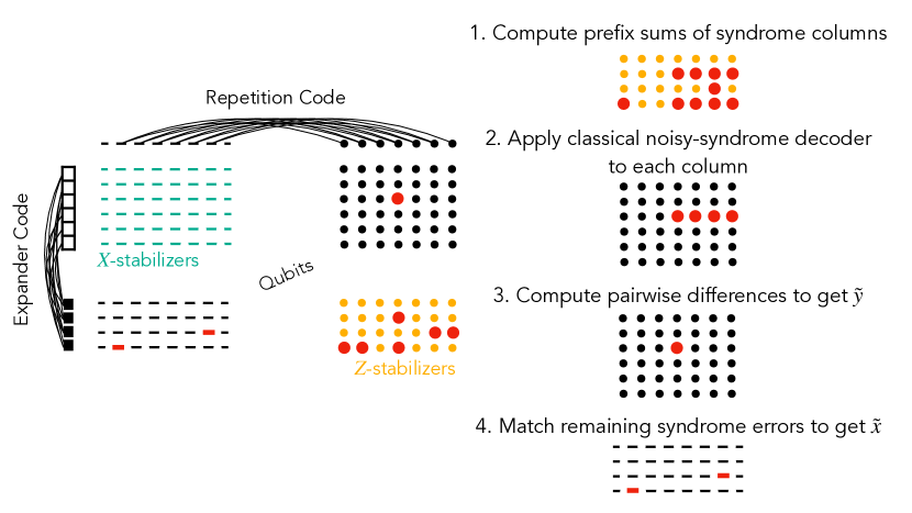
Figure 1: Illustration of our decoding algorithm in Theorem 21 for the hypergraph product of a classical expander-based LDPC code with a repetition code. The hypergraph product is drawn on the left; there are two matrices of qubits, corresponding to $x$ and $y$ respectively in the proof sketch of Theorem 21, where the errors are supported on the qubits marked by red dots. The support of the $Z$-syndrome $s=\partial_{1}^{\mathcal{C}}(x,y)=(I\otimes\partial^{\mathcal{B}})x+(\partial^{\mathcal{A}}\otimes I)y$ is also marked by red dots within the matrix of $Z$-stabilizers (i.e. parity checks of the boundary map $\partial_{1}^{\mathcal{C}}$). The algorithm outputs an estimate $(\tilde{x},\tilde{y})$ for the true error $(x,y)$.

Proof sketch of Theorem 21.

By the symmetry of $\mathcal{C}_{*}$ and its cochain complex $\mathcal{C}^{*}$ (see Definition 14), it suffices to describe the decoder $D_{0}:C_{0}\rightarrow C_{1}$ as described in Definition 13; the construction of $D^{2}:C^{2}\rightarrow C^{1}$ will be exactly analogous. Thus, if we fix some error $c=(x,y)\in C_{1}=A_{0}\otimes\mathbb{F}_{2}^{\ell}\oplus A_{1}\otimes\mathbb{F}_{2}^{\ell}$, our goal is to construct an efficient algorithm $D_{0}(s)$ that receives as input the syndrome

$$s=\partial_{1}^{\mathcal{C}}(c)=(I\otimes\partial^{\mathcal{B}})x+(\partial^{\mathcal{A}}\otimes I)y,$$ (1)

and outputs some $\tilde{c}\in C_{1}$ that differs from $c$ by an element $\tilde{c}-c\in\operatorname{im}\partial_{2}^{\mathcal{C}}$. In fact, we can define $e=\Theta(\min\{N^{\mathcal{A}},\ell\})$ to be sufficiently small compared to the distance of $\mathcal{C}$ so that it suffices to output any $\tilde{c}$ of weight $|\tilde{c}|\leq O(|c|)$ such that $\partial_{1}^{\mathcal{C}}\tilde{c}=s$.

For $i\in\{0,1\}$, let $N_{i}=\dim A_{i}$, so that $A_{i}\otimes\mathbb{F}_{2}^{\ell}\cong\mathbb{F}_{2}^{N_{i}\times\ell}$ can be viewed as the space of $N_{i}\times\ell$ matrices over $\mathbb{F}_{2}$.

First observe that if $x=0$, then $s=(\partial^{\mathcal{A}}\otimes I)y$ is simply the matrix whose columns are syndromes of the columns of $y$ under the parity-check matrix $\partial^{\mathcal{A}}$ of $\mathcal{A}$. By the assumption that $\mathcal{A}$ has an efficient noisy-syndrome decoder $D^{\mathcal{A}}:A_{0}\rightarrow A_{1}$, so we can simply apply $D^{\mathcal{A}}$ to each column of $s$ independently to recover $y$. Note that here we did not even need the ability of $D^{\mathcal{A}}$ to accomodate noisy syndromes.

Now in the general case where $x\neq 0$, then we can interpret $s=(I\otimes\partial^{\mathcal{B}})x+(\partial^{\mathcal{A}}\otimes I)y$ as being the matrix whose columns are noisy syndromes of the columns of $y$ under the parity-check matrix $\partial^{\mathcal{A}}$, where $(I\otimes\partial^{\mathcal{B}})x$ provides the syndrome errors. Letting $a_{i}$ denote the $i$th column of a matrix $a$, then observe that $((I\otimes\partial^{\mathcal{B}})x)_{i}=x_{i-1}+x_{i}$, where we view $[\ell]\cong\mathbb{Z}/\ell\mathbb{Z}$ so that $i-1$ is taken$\pmod{\ell}$.

Therefore an initial attempt at decoding would be to again apply $D^{\mathcal{A}}$ to each column of $s$. This would yield a matrix with columns $D^{\mathcal{A}}(s_{i})$ satisfying $|D^{\mathcal{A}}(s_{i})-y_{i}|\leq O(|x_{i-1}+x_{i}|)$ by the definition of noisy-syndrome decodability. However, it is not clear that we have made any progress, as we simply know that the matrix with columns $D^{\mathcal{A}}(s_{i})$ differs from $y$ in at most $\sum_{i}O(|x_{i-1}+x_{i}|)\leq O(|x|)$ positions. Because we could have $|x|=\Theta(|y|)=\Theta(e)$, the all-zeros matrix could provide an equally good approximation to $y$.

Thus we need a way to isolate, or amplify, the effect of the errors $y$ while suppressing the syndrome errors from $x$, so that we can gain more information from our noisy-syndrome decoder $D^{\mathcal{A}}$. The solution is to apply $D^{\mathcal{A}}$ to prefix sums of $s$. That is, for every $k\in[\ell+1]$, we compute

$$\tilde{a}_{k}=D^{\mathcal{A}}\Bigl{(}\sum_{i\in[k]}s_{i}\Bigr{)},$$ (2)

which we hope to be a good approximation to the true prefix sums $a_{k}=\sum_{i\in[k]}y_{i}$.

The key observation here is that while passing to these prefix sums potentially allows an error in some column $y_{i}$ to propagate to all $a_{k}$ for $k>i$, the contribution of errors in $x$ to prefix sums of the syndrome $s$ is not amplified. Formally, by definition $\sum_{i\in[k]}((I\otimes\partial^{\mathcal{B}})x)_{i}=\sum_{i\in[k]}(x_{i-1}+x_{i})=x_{-1}+x_{k-1}$ (where $x_{-1}=x_{-1\pmod{\ell}}=x_{\ell-1}$). Thus if $x_{-1}=0$, then $x$ contributes at most $|x|$ nonzero entries to the matrix whose $k$th column is the prefix sum $\sum_{i\in[k]}s_{i}$. We can guarantee that $x_{-1}=0$ by permuting the columns of all matrices by an appropriate (e.g. random) cyclic shift. We obtain the randomized decoder in Theorem 21 by trying a small number of random cyclic shifts, while we obtain the deterministic decoder by trying all $\ell$ possible cyclic shifts.

Thus by the definition of noisy-syndrome decoding, it must hold that

$$\sum_{k\in[\ell+1]}|\tilde{a}_{k}-a_{k}|\leq O(|x|).$$ (3)

Note that here we are able to apply $(\Theta(n),\Theta(n),\Theta(1))$-noisy-syndrome decoding because $|x|$ (which bounds the syndrome errors) and each $|a_{k}|\leq|y|$ (which bounds the code bit errors) are by assumption bounded above by $e\leq\Theta(n)$.

Therefore after computing $\tilde{a}_{k}$ for every $k\in[\ell+1]$, our decoder computes an estimate $\tilde{y}\in\mathbb{F}_{2}^{N_{1}\times\ell}$ by letting the $k$th column be $\tilde{y}_{k}:=\tilde{a}_{k+1}-\tilde{a}_{k}$. Tracing through the definitions, we see that $\tilde{y}-y=(I\otimes\partial^{\mathcal{B}})b$ for the matrix $b\in\mathbb{F}_{2}^{N_{1}\times\ell}$ given by $b_{k}:=\tilde{a}_{k+1}-a_{k+1}$, as for every $k$ we have $(\tilde{y}-y)_{k}=b_{k-1}+b_{k}$.

Therefore we have shown that $\tilde{y}=y+(I\otimes\partial^{\mathcal{B}})b$ for a matrix $b$ satisfying $|b|\leq O(|x|)$ by (3). Thus our decoder simply computes the minimum possible weight $\tilde{x}\in\mathbb{F}_{2}^{N_{0}\times\ell}$ such that $\partial_{1}^{\mathcal{C}}(\tilde{x},\tilde{y})=s$, or equivalently, such that $(I\otimes\partial^{\mathcal{B}})\tilde{x}=s-(\partial^{\mathcal{A}}\otimes I)\tilde{y}$. It then outputs $\tilde{c}:=(\tilde{x},\tilde{y})$. As $\tilde{x}^{\prime}=x-(\partial^{\mathcal{A}}\otimes I)b$ is a valid such choice of $\tilde{x}$, the decoder is guaranteed to output $\tilde{c}$ of weight $|\tilde{c}|=|\tilde{x}|+|\tilde{y}|\leq O(|x|+|y|)$, as desired. ∎

3.2 Decoding Lifted Products

In this section, we outline the main ideas in our proof of Theorem 1, which provides a decoding algorithm for the nearly-linear-distance lifted-product codes in Theorem 20. This algorithm is one of the main technical contributions of our paper.

We first reiterate Theorem 1 in slightly more technical terms:

Theorem 22 (Informal statement of Theorem 32).

For some $\ell\in\mathbb{N}$ that is a power of $2$, define $\mathcal{A}^{(\ell)}$, $\mathcal{B}^{(\ell)}$, and $\mathcal{C}^{(\ell)}$ as in Theorem 20. Let $N=\ell\log\ell$, and assume that $\mathcal{A}^{(\ell)}_{*}$ and its cochain complex ${\mathcal{A}^{(\ell)}}^{*}$ are both $(\Theta(N),\Theta(N),\Theta(1))$-noisy-syndrome decodable in time $O(N)$. Then for every $0<\epsilon\leq 1/2$ and every $\delta>0$, there exists a randomized decoder for $\mathcal{C}^{(\ell)}$ that protects against $e=\Theta(\epsilon\ell)$ adversarial errors with failure probability $\leq\delta$ and runs in time $O(N^{2+2\epsilon}\cdot\log(1/\delta))$.

In Theorem 22, we assume that $\ell$ is a power of $2$ to avoid rounding issues in one step of the proof, but we believe that the algorithm can be extended to accomodate all $\ell\in\mathbb{N}$.

As described in Remark 12 above, we expect many expander-based $[\Theta(N),\Theta(N),\Theta(N)]$ classical LDPC codes to be $(\Theta(N),\Theta(N),\Theta(1))$-noisy-syndrome decodable, and we prove the precise statement we need in Proposition 24.

Below, we outline the main ideas in our proof of Theorem 22. For the full details, the reader is referred to Section 6.

Proof sketch of Theorem 22.

At a high level, we follow the idea of applying noisy-syndrome decoding to prefix sums of the received syndrome, as was described in Section 3.1 above for the proof of Theorem 21. However, the prefix sums in the lifted product case rapidly become too high-weight to apply the noisy-syndrome decoder $D^{\mathcal{A}}$ of $\mathcal{A}$. We must instead start by taking prefix sums of constant size, and then iteratively passing larger prefix sums through $D^{\mathcal{A}}$ to obtain successively better approximations to the true error. Each successive improvement in our error approximation allows us to take an even larger prefix sum without overloading the error tolerance of $D^{\mathcal{A}}$. We can ultimately arrive at a true decoding after $\Theta(\log\ell)$ of these iterations. However, each iteration has a constant probability of failure, as we must sample a random cyclic shift in like in Theorem 21. Thus we obtain an overall success probability of $2^{-\Theta(\log\ell)}=1/\operatorname{poly}(\ell)$, which we amplify by repeating the algorithm $\operatorname{poly}(\ell)$ times.

We now provide more details. Fix $\ell\in\mathbb{N}$, and let $\mathcal{A}=\mathcal{A}^{(\ell)}$, $\mathcal{B}=\mathcal{B}^{(\ell)}$, and

$$\mathcal{C}_{*}=\mathcal{C}_{*}^{(\ell)}=(\mathcal{A}\otimes_{R_{\ell}}\mathcal{B})_{*}=\left(A_{1}\xrightarrow{\partial^{\mathcal{A}}+(1+X)}A_{0}\oplus A_{1}\xrightarrow{(1+X)+\partial^{\mathcal{A}}}A_{0}\right).$$

By the symmetry of $\mathcal{C}_{*}$ and $\mathcal{C}^{*}$, it suffices to construct the decoder $D_{0}:C_{0}\rightarrow C_{1}$ described in Definition 13, as the decoder $D^{2}:C^{2}\rightarrow C^{1}$ will be exactly analogous.

Thus fix some error $c=(x,y)\in C_{1}=A_{0}\oplus A_{1}$. Our goal is to construct an efficient algorithm $D_{0}(s)$ that receives as input the syndrome

$$s=\partial_{1}^{\mathcal{C}}=(1+X)x+\partial^{\mathcal{A}}y,$$

and outputs some $\tilde{c}\in C_{1}$ for which $\tilde{c}-c\in\operatorname{im}\partial_{2}^{\mathcal{C}}$. In fact, we can define $e=\Theta(\epsilon\ell)$ to be sufficiently small compared to the distance $\Theta(\ell)$ of $\mathcal{C}$ so that it suffices to output any $\tilde{c}$ of weight $|\tilde{c}|\leq O(|c|)$ such that $\partial_{1}^{\mathcal{C}}\tilde{c}=s$.

Similarly to the proof of Theorem 21, if $x=0$, then $s=\partial^{\mathcal{A}}y$, so we can simply apply $D^{\mathcal{A}}$ to $s$ to recover $y$. Moving to the general case where $x\neq 0$, we can view $(1+X)x$ as a syndrome error and $y$ as a code error, which both contribute to the noisy syndrome $s=(1+X)x+\partial^{\mathcal{A}}y$.

A natural approach is to follow our proof of Theorem 21 and apply $D^{\mathcal{A}}$ to prefix sums of $s$. Specifically, the natural analogue of (2) in the lifted product setting is to define $\tilde{a}_{k}$ for $k\in[\ell+1]$ by

$$\tilde{a}_{k}=D^{\mathcal{A}}\Bigl{(}\sum_{i\in[k]}X^{i}s\Bigr{)},$$ (4)

which we hope to be a good approximation to $a_{k}:=\sum_{i\in[k]}X^{i}y$.

To see that multiplying by $\sum_{i\in[k]}X^{i}$ is the natural lifted-product analogue of the prefix sums for the hypergraph product, observe that multiplying a vector by $\sum_{i\in[k]}X^{i}$ simply sums together $k$ cyclic shifts of that vector. But the length-$k$ prefix sums considered in Section 3.1 can similar be obtained summing together $k$ cyclic shifts of the columns of the relevant matrices. Thus in both cases, the prefix sums are obtained by summing together shifts of the relevant vectors or matrices under the cyclic group action they inherit from the repetition code.

Now, we see that the prefix sum $\sum_{i\in[k]}X^{i}s$ receives a contribution of $\partial^{\mathcal{A}}(\sum_{i\in[k]}X^{i}y)$ from $y$. As $|y|$ can be as large as $e=\Theta(\epsilon\ell)=\Theta(\epsilon N/\log N)$, the prefix sum $\sum_{i\in[k]}X^{i}y$ can have weight $>\omega(N)$ for any $k>\omega(\log N)/\epsilon$. Thus unless $k\leq O(\log N)/\epsilon$ (it is helpful to think of $\epsilon>0$ as a constant here), $\sum_{i\in[k]}X^{i}s$ will represent the noisy syndrome of an error that may be too large for $D^{\mathcal{A}}$ to decode. In contrast, if we were to use a similar algorithm as in the proof of Theorem 21, we would want to compute $\tilde{a}_{k}$ at least up to $k=\Theta(N/\log N)$.

We resolve this issue by initially only computing $\tilde{a}_{k}$ in (4) for all $1\leq k\leq t$ for a constant $t=t_{0}$ (we in fact take $t_{0}=2$, but for now it may be helpful to think of $t$ as a large constant, or even as a slowly growing function of $N$). We then form an initial estimate $\tilde{z}\in A_{1}$ for $y$ using these vectors $\tilde{a}_{k}$ for $1\leq k\leq t$, similarly as in the proof of Theorem 21.

Specifically, letting $A_{1}=R_{\ell}^{n_{1}}$, then we can index the $n_{1}\cdot\ell$ bits in a vector $v\in A_{1}$ by pairs $(h,k)\in[n_{1}]\times[\ell]$, such that $(X^{i}v)_{h,k}=v_{h,k+i}$, where we take the second subscript modulo $\ell$. Then for $h\in[n_{1}]$ and $m\in[\ell/t]$, we define

$$\tilde{z}_{h,mt+i}:=\begin{cases}0,&i=0\\ (\tilde{a}_{i+1})_{h,mt}-(\tilde{a}_{i})_{h,mt},&1\leq i\leq t-1.\end{cases}$$

Assume that we had initially performed a random cyclic shift on all vectors above, by multiplying all vectors by $X^{j}$ for a random $j\in[\ell]$, to avoid accumulation of errors on the components $(\tilde{a}_{i})_{h,mt}$ that we use above. Then using a similar argument as in the proof of Theorem 21, we apply the definition of noisy-syndrome decoding to show that with constant probability, $\tilde{z}_{h,mt+i}$ is a good approximation to $y_{h,mt+i}$ across all $h\in[n_{1}]$, $m\in[\ell/t]$, and $1\leq i<t$. However, we do not obtain an estimate of the components $y_{h,mt+i}$ for $i=0$. These “gaps” in our estimate $\tilde{z}$ occur periodically in one out of every $t$ components, and arise from the fact that we only computed $t$ prefix sums $\tilde{a}_{k}$.

As these gaps in our estimate $\tilde{z}$ occur at a one out of every $t$ of the positions, where we have chosen $t$ to be a constant, we must find a way to “fill in” these gaps to obtain a better estimate of $y$. For this purpose, observe that we have good estimates $\tilde{z}_{h,mt+k}$ of $y_{h,mt+k}$ for all $h,m$ and all $1\leq k<t$, and we also have good estimates $(\tilde{a}_{t})_{h,mt-k}$ of $(a_{t})_{h,mt-k}=\sum_{i\in[t]}y_{h,mt-k+i}$ for all $h,m,k$. Therefore, for $k\in[t]$, we should expect $b_{h,mt-k}:=(a_{t})_{h,mt-k}-\sum_{i\in[t]}\tilde{z}_{h,mt-k+i}$ to be a good estimate of $y_{h,mt}$. We thus define $\tilde{r}\in A_{1}$ by letting $\tilde{r}_{h,mt}$ be the majority value of $b_{h,mt-k}$ across all $k\in[t]$, and letting $\tilde{r}_{h,mt+i}=0$ for all $1\leq i<t$. We then let $\tilde{y}_{1}:=\tilde{z}+\tilde{r}$ be our estimate of $y$.

We show that the error $\tilde{y}_{1}-y$ in our approximation $\tilde{y}_{1}$ of $y$ can be expressed in the form $\tilde{y}_{1}-y=(1+X)u+r^{\prime}$, where $|u|\leq O(\ell)$ and $|r^{\prime}|\leq O(\ell/t)$ (see the proof of Proposition 37 for details). Now consider taking a prefix sum of this error $y-\tilde{y}_{1}$ of any length $k\in[t_{1}]$ for $t_{1}=2t=2t_{0}$. As

$$\Bigl{|}\sum_{i\in[k]}X^{i}(y-\tilde{y}_{1})\Bigr{|}=\Bigl{|}(1+X^{k})u+\sum_{i\in[2k]}X^{i}r^{\prime}\Bigr{|}\leq 2|u|+2t|r^{\prime}|\leq O(\ell),$$

this prefix sum will not overload the noisy-syndrome decoder $D^{\mathcal{A}}$. Thus we can compute new decodings $\tilde{a}_{k}^{\prime}:=D^{\mathcal{A}}(\sum_{i\in[k]}X^{i}(s-\partial^{\mathcal{A}}\tilde{y}_{1}))$ of the length-$k$ prefix sums of $s-\partial^{\mathcal{A}}\tilde{y}_{1}$ for all lengths $k\in[t_{1}]$, and repeat the entire procedure described above to obtain a new estimate $\tilde{y}_{2}$ for $y$. After iterating $\Theta(\log\ell)$ times, we show that the error term $r^{\prime}$ described above vanishes, at which point we have recovered some $\tilde{y}$ for which $\tilde{y}-y=(1+X)u$, where $|u|\leq O(\ell)$. Similarly as in the proof of Theorem 21, the decoder can then compute the minimum possible weight $\tilde{x}\in A_{0}$ for which $\partial_{1}^{\mathcal{C}}(\tilde{x},\tilde{y})=s$. We show that the resulting estimate $\tilde{c}:=(\tilde{x},\tilde{y})$ must lie in $c+\operatorname{im}\partial_{2}^{\mathcal{C}}$, as desired.

Note that the random cyclic shift in each iteration mentioned above introduces a constant failure probability, so the $\Theta(\log\ell)$ iterations collectively have a $2^{-\Theta(\log\ell)}=1/\operatorname{poly}(\ell)$ success probability. We amplify this sucess probability be repeating the entire algorithm $\operatorname{poly}(\ell)$ times. ∎

Our decoding algorithm described above shares some similarities with proof of distance in Theorem 20 shown by [PK22b]. In particular, [PK22b] also computed prefix sums $\sum_{i\in[k]}X^{i}c$ of errors $c$ to prove the $\Omega(\ell)$ bound on distance, and relied on expansion of the graphs underlying the Tanner codes $\mathcal{A}^{(\ell)}$. However, there are significant differences between the two results. Perhaps the most fundamental difference lies in the iterative nature of our decoding algorithm in Theorem 22, which is absent from the distance proof of [PK22b]. Interestingly, the greedy flip-style decoding algorithms for asymptotically good qLDPC codes more closely mirror their distance proofs (see e.g. [LZ23, DHLV23]).

4 Classical Tanner Codes and Noisy-Syndrome Decodability

In this section, we describe classical Tanner codes obtained by imposing the constraints of a good local code around each vertex of an expander graph [SS96]. Furthermore, we follow [PK22b] in constructing these codes to respect a large cyclic group symmetry. We show that the chain complexes from these codes, along with their associated cochain complexes, are noisy-syndrome decodable in linear time (see Section 2.4). Applying such chain complexes in a lifted product construction yields the nearly-linear distance codes of [PK22b], which we show how to decode in Section 6.

Distance proofs for Tanner codes have been previously established (e.g. [SS96]), while decoding algorithms for such codes have been given both without (e.g. [SS96, Zem01, LZ23]) and with (e.g. [Spi96, GTC⁺23]) syndrome noise. However, for completeness we provide proofs of the noisy-syndrome decodability properties we require in Appendix B, as we were unable to find the precise statements we need in the prior literature. For instance, [Spi96] proves noisy-syndrome decodability for the chain complexes associated to classical Tanner codes, but not for the associated cochain complexes. Meanwhile, [GTC⁺23] proves an analogue of noisy-syndrome decodability (i.e. single-shot decodability) for the 3-term chain and cochain complexes associated to quantum Tanner codes [LZ22, LZ23], but not for the 2-term complexes associated to classical Tanner codes.

Remark 23.

We use classical LDPC codes given by imposing local codes around each vertex of a spectral expander graph [SS96], because as shown by [PK22b], such codes can be made to respect a large cyclic group symmetry using known symmetric spectral expander constructions [ACKM19, JMO⁺22]. However, as mentioned above, the chain and cochain complexes of such codes have slightly different structures. In contrast, classical LDPC codes can alternatively be constructed using a different type of expanders called twosided lossless expanders. The chain and cochain complexes for such codes have the same structure and hence can be decoded with the same algorithm (see e.g. [SS96]). However, it remains an open question to construct twosided lossless expanders respecting a large group symmetry (see for instance [CRVW02, LH22, CRTS23, Gol24]).

The result below describes the specific 2-term chain complexes we need, which we will construct using classical Tanner codes.

Proposition 24.

There exist positive constants $w,\alpha,\beta,e_{0},e_{1},\gamma$ for which the following holds: there is an explicit infinite family of 2-term chain complexes $\mathcal{A}^{(\ell)}=(A_{1}^{(\ell)}\xrightarrow{\partial^{(\ell)}}A_{0}^{(\ell)})$ indexed by $\ell\in\mathbb{N}$, such that each $\mathcal{A}^{(\ell)}$ has the following properties:

1. $\mathcal{A}^{(\ell)}$ is a 2-term chain complex over $R_{\ell}$ of locality $w$.

2. Letting $n_{i}=\dim_{R_{\ell}}A^{(\ell)}_{i}$, then $n_{0},n_{1},n_{1}-n_{0}=\Theta(\log\ell)$ (so that $\dim_{\mathbb{F}_{2}}A^{(\ell)}_{i}=\Theta(\ell\log\ell)$).

3. Both the chain complex $\mathcal{A}^{(\ell)}_{*}$ and its cochain complex ${\mathcal{A}^{(\ell)}}^{*}$ are $(\alpha,\beta)$-expanding, and are $(e_{0},e_{1},\gamma)$-noisy-syndrome decodable in time $O(\ell\log\ell)$ for $e_{0},e_{1}=\Theta(\ell\log\ell)$.

[PK22b] showed that the 2-term chain complexes such as those in Proposition 24 can be used to obtain lifted product quantum codes of nearly linear distance. However, the 2-term chain complexes used in [PK22b] were based on expander graphs from random abelian lifts [ACKM19]. These random expanders were later derandomized in [JMO⁺22], which we use to obtain the explicit construction in Proposition 24. Theorem 20 above follows directly by applying the results of [PK22b] with the graphs constructed in [JMO⁺22]. Note that all of our results also go through using the random abelian lifts of [ACKM19], at the cost of explicitness.

One of our main contributions (Theorem 1, proven in Section 6) is to efficiently decode the codes in Theorem 20 up to adversarial corruptions of linear weight with respect to the code’s distance.

We prove Proposition 24 in Appendix B. In particular, Appendix B contains an essentially self-contained proof of the linear-time noisy-syndrome decodability of the chain and cochain complexes associated to classical Tanner codes. This noisy-syndrome decodability is the main property we need that [PK22b] does not consider.

5 Hypergraph Product of Tanner Code and Repetition Code

In this section, we present an efficient decoding algorithm for the hypergraph product (see Section 2.6) of an expanding classical LDPC code with a repetition code. For instance, the hypergraph product of a $[N,\Theta(N),\Theta(N)]$ Tanner code with a $[\Theta(N),1,\Theta(N)]$ repetition code is a $[[\Theta(N^{2}),\Theta(N),\Theta(N)]]$ quantum code, for which our decoding algorithm can efficiently recover from $\Theta(N)$ adversarial errors.

5.1 Result Statement

Our main result on decoding the hypergraph product of a Tanner code and a repetition code is stated below.

Theorem 25.

Let $\mathcal{A}_{*}=(A_{1}\xrightarrow{\partial^{\mathcal{A}}}A_{0})$ be a 2-term chain complex of locality $w$ such that $\mathcal{A}_{*}$ and $\mathcal{A}^{*}$ are both $(e_{0},e_{1},\gamma)$-noisy-syndrome decodable in time $T$. For some $\ell\in\mathbb{N}$, let $\mathcal{B}_{*}=(B_{1}\xrightarrow{\partial^{\mathcal{B}}}B_{0})$ be the 2-term chain complex over $R_{\ell}$ given by $B_{0}=B_{1}=R_{\ell}$ and $\partial^{\mathcal{B}}=1+X\in R_{\ell}$. Let

$$\mathcal{C}_{*}=\mathcal{A}\otimes_{\mathbb{F}_{2}}\mathcal{B}$$

denote the hypergraph product. Let $d(\mathcal{C})$ denote the distance of the quantum code associated to $\mathcal{C}_{*}$, and let $N^{\mathcal{A}}=\dim A_{0}+\dim A_{1}$. Then for every $\delta>0$, there exists a randomized decoder for this quantum code that protects against $e=\min\{e_{0},\;e_{1},\;\ell/2,\;(d(\mathcal{C})-1)/(2+(w+2)\gamma)\}$ adversarial errors, runs in time $O((N^{\mathcal{A}}+T)\ell\log(1/\delta))$, and has failure probability $\leq\delta$. Furthermore, there exists a deterministic decoder protecting against $e$ errors that runs in time $O((N^{\mathcal{A}}+T)\ell^{2})$.

While we define the chain complex $\mathcal{B}$ as a chain complex over $R_{\ell}$ for notational convenience, in this section we do not assume that $\mathcal{A}$ has an $R_{\ell}$-structure, and we take the hypergraph product over $\mathbb{F}_{2}$. We do consider decoding a lifted product over $R_{\ell}$ in Section 6.

The chain complex $\mathcal{B}_{*}=(R_{\ell}\xrightarrow{1+X}R_{\ell})$ and its cochain complex $\mathcal{B}^{*}=(R_{\ell}\xleftarrow{1+X^{\ell-1}}R_{\ell})$ both have associated classical code given by the length-$\ell$ repetition code. The parity checks simply check that every pair of consecutive code bits are equal. We reiterate that $X$ here denotes an indeterminate variable in polynomials, rather than a Pauli operator.

Example 26.

As an example application of Theorem 25 above, consider an instantiation of $\mathcal{C}=\mathcal{A}\otimes_{\mathbb{F}_{2}}\mathcal{B}$ where $\mathcal{A}$ is the 2-term chain complex associated to asymptotically good classical Tanner codes such as those given in Proposition 24, and $\mathcal{B}$ is defined by letting $\ell=\Theta(N^{\mathcal{A}})$. Note that we could alternatively let $\mathcal{A}$ be the 2-term chain complex associated to a random lossless expander code (see e.g. [SS96]).

Then the Künneth formula (Proposition 15) implies that $\mathcal{C}$ has associated quantum code dimension

$$\dim(H_{1}(\mathcal{C}))=\dim(H_{1}(\mathcal{A}))\cdot\dim(H_{0}(\mathcal{B}))+\dim(H_{0}(\mathcal{A}))\cdot\dim(H_{1}(\mathcal{B}))=\Theta(N^{\mathcal{A}}),$$

as $\dim(H_{1}(\mathcal{A}))=\dim\ker(\partial^{\mathcal{A}})\geq\dim(A_{1})-\dim(A_{0})=\Theta(N^{\mathcal{A}})$ by Proposition 24, $\dim(H_{0}(\mathcal{A}))\leq O(N^{\mathcal{A}})$ by definition, $\dim(H_{0}(\mathcal{B}))=\ell-\dim(\operatorname{im}\partial^{\mathcal{B}})=1$ because $\operatorname{im}\partial^{\mathcal{B}}$ is by definition the set of all vectors in $\mathbb{F}_{2}^{\ell}$ of even Hamming weight, and $\dim(H_{1}(\mathcal{B}))=\dim(H^{0}(\mathcal{B}))=\dim(H_{0}(\mathcal{B}))=1$ by the symmetry of $\mathcal{B}$.

Meanwhile, the classical codes associated to $\mathcal{A}_{*}$ and $\mathcal{A}^{*}$ have distance $\Theta(N^{\mathcal{A}})$ by Proposition 24, and the classical codes associated to $\mathcal{B}_{*}$ and $\mathcal{B}^{*}$ are both length-$\ell$ repetition codes, which have distance $\ell=\Theta(N^{\mathcal{A}})$. Thus Proposition 16 implies that the quantum code associated to $\mathcal{C}$ has distance

$$d(\mathcal{C})\geq\Theta(N^{\mathcal{A}}).$$

The above bound is in fact tight up to constant factors; see for instance Theorem 15 of [TZ14].

Thus $\mathcal{C}$ is a $[[N=\Theta(N^{\mathcal{A}})^{2},\;K=\Theta(N^{\mathcal{A}}),\;D=\Theta(N^{\mathcal{A}})]]$ quantum LDPC code, for which Theorem 25 provides a $O(N\log(1/\delta))$-time randomized decoder against $\Theta(D)$ adversarial errors with failure probability $\delta$, as well as a $O(N^{3/2})$-time deterministic decoder against $\Theta(D)$ adversarial errors.

We prove Theorem 25 in the following sections. Section 5.2 below presents a decoding algorithm for $\mathcal{C}$ (Algorithm 1) that takes as input a parameter $j\in[\ell]$; in Section 5.3, we show that this decoding algorithm succeeds for at least half of all choices of $j\in[\ell]$. Section 5.4 analyzes the running time of this algorithm. Section 5.5 then combines these results to prove Theorem 25, simply using repeated runs of Algorithm 1 for different choices of $j\in[\ell]$.

5.2 Decoder With Constant Probability of Success

In this section, we present Algorithm 1, which contains the technical core of the decoding algorithm we use to prove Theorem 25. Specifically, Algorithm 1 can be used to successfully decode the code $\mathcal{C}_{*}$ in Theorem 25 with probability $\geq 1/2$. In Section 5.5 below, we show how to amplify this success probability to prove Theorem 25.

By symmetry of the construction

$$\mathcal{C}_{*}=\mathcal{A}\otimes\mathcal{B}=\left(A_{1}\otimes R_{\ell}\xrightarrow{\partial^{\mathcal{A}}\otimes I+I\otimes(1+X)}A_{0}\otimes R_{\ell}\oplus A_{1}\otimes R_{\ell}\xrightarrow{I\otimes(1+X)+\partial^{\mathcal{A}}\otimes I}A_{0}\otimes R_{\ell}\right).$$

in Theorem 25, it will suffice to provide the decoding algorithm $D_{0}:C_{0}\rightarrow C_{1}$ described in Definition 13, as the decoding algorithm $D^{2}:C^{2}\rightarrow C^{1}$ will be exactly analogous. Note that all tensor products $\otimes$ in the equation above are implicitly taken over $\mathbb{F}_{2}$.

We let $D^{\mathcal{A}}:A_{0}\rightarrow A_{1}$ be an $(e_{0},e_{1},\gamma)$-noisy-syndrome decoder for the classical code associated to $\mathcal{A}$ that runs in time $\leq T$; such a decoder is assumed to exist in the statement of Theorem 25.

For a given error $c\in C_{1}=A_{0}\otimes R_{\ell}\oplus A_{1}\otimes R_{\ell}$ of weight $|c|\leq e$, the decoder $D_{0}$ receives as input the syndrome $s=\partial_{1}^{\mathcal{C}}c\in C_{0}=A_{0}\otimes R_{\ell}$. The decoder’s goal is to output an element $\tilde{c}\in C_{1}$ that lies in the coset $c+B_{1}(\mathcal{C})$. We will define $D_{0}(s)$ to simply perform several appropriate calls to Algorithm 1.

1

2

Input : Syndrome $s\in C_{0}$ of some error $c=(x,y)\in C_{1}$, and some $j\in[\ell]$

Output : $\tilde{c}\in C_{1}$ that will be shown to be a low-weight element of $c+B_{1}(\mathcal{C})$ for at least half of all choices of $j\in[\ell]$, as long as $|c|$ is sufficiently small

3

4Function DecHGP($s,j$):

5       Decomposing $s=\sum_{i\in[\ell]}s_{i}\otimes X^{i}$, then for each $k\in[\ell+1]$, compute

$$\tilde{a}_{j+k}:=D^{\mathcal{A}}\left(\sum_{i\in[k]}s_{j+i\pmod{\ell}}\right)$$

6       Define $\tilde{y}\in A_{1}\otimes R_{\ell}$ by $\tilde{y}:=\sum_{k\in[\ell]}(\tilde{a}_{j+k+1}-\tilde{a}_{j+k})\otimes X^{j+k}$

7       Compute the element $\tilde{x}\in A_{0}\otimes R_{\ell}$ of minimum weight such that $\partial_{1}^{\mathcal{C}}(\tilde{x},\tilde{y})=s$. If no such $\tilde{x}$ exists, return FAIL.

8       return $\tilde{c}:=(\tilde{x},\tilde{y})$

9      

Algorithm 1 Algorithm to decode hypergraph product of Tanner and repetition code.

Note that in line 1 of Algorithm 1, $X^{j+k}=X^{j+k\pmod{\ell}}$ by the definition of $R_{\ell}=\mathbb{F}_{2}[X]/(X^{\ell}-1)$.

Proposition 27 below implies that if $|c|$ is sufficiently small, then the procedure DecHGP($s,j$) in Algorithm 1 outputs a correct low-weight decoding $\tilde{c}\in c+B_{1}(\mathcal{C})$ for at least half of all possible choices of $j\in[\ell]$. Thus if we let $D_{0}(s)$ simply run DecHGP($s,j$) for a small number of random $j\in[\ell]$, it will obtain a correct decoding $\tilde{c}\in c+B_{1}(\mathcal{C})$ with high probability. Meanwhile, if we instead let $D_{0}(s)$ run DecHGP($s,j$) for all $j\in[\ell]$, it will (with a slightly larger time overhead) deterministically obtain a correct decoding $\tilde{c}$. The precise details for defining and analyzing $D_{0}$ in both of these cases are provided in Section 5.5.

5.3 Correctness of the Constant-Success-Probability Decoding Algorithm

In this section, we show correctness for the decoder $D_{0}$ presented in Section 5.2. Formally, we show the following.

Proposition 27.

Define all variables as in Theorem 25. For every error $c\in C_{1}$ of weight $|c|\leq e$, letting $s=\partial_{1}^{\mathcal{C}}c$, then it holds for $\geq\ell/2$ of all $j\in[\ell]$ that the procedure DecHGP($s,j$) in Algorithm 1 outputs some $\tilde{c}\in C_{1}$ satisfying $\partial_{1}^{\mathcal{C}}\tilde{c}=s$ and $|\tilde{c}|\leq((w+2)\gamma+1)e$.

Proof.

We first fix some notation. For an $\mathbb{F}_{2}$-vector space $V$ and an element $v\in V\otimes_{\mathbb{F}_{2}}R_{\ell}$, we let $v=\sum_{i\in[\ell]}v_{i}\otimes X^{i}$ be the natural decomposition.

Fix any $c=(x,y)\in A_{0}\otimes R_{\ell}\oplus A_{1}\otimes R_{\ell}$ such that $|c|\leq e$. Recall here that all Hamming weights are computed with respect to the $\mathbb{F}_{2}$-structure, by counting the number of nonzero bits of the specified vector in its representation in the chosen $\mathbb{F}_{2}$-basis. By assumption $|x|\leq|c|\leq\ell/2$, so it holds for $\geq\ell/2$ of all $j\in[\ell]$ that $x_{j-1\pmod{\ell}}=0$. For the remainder of the proof we assume that $j$ satisfies $x_{j-1\pmod{\ell}}=0$.

For $k\in[\ell+1]$, let $a_{j+k}=\sum_{i\in[k]}y_{j+i\pmod{\ell}}$ denote the prefix sums of $y$. Intuitively, the $\tilde{a}_{j+k}$ defined in line 1 of Algorithm 1 provide approximations to these prefix sums. The claim below bounds the error in this approximation.

Claim 28.

It holds that $\sum_{k\in[\ell+1]}|\tilde{a}_{j+k}-a_{j+k}|\leq\gamma|x|$ and $\tilde{a}_{j}-a_{j}=\tilde{a}_{j+\ell}-a_{j+\ell}=0$.

Proof of Claim 28.

By definition each $s_{i}=x_{i-1\pmod{\ell}}+x_{i}+\partial^{\mathcal{A}}y_{i}$. Therefore for $k\in[\ell+1]$, because $x_{j-1\pmod{\ell}}=0$, it follows that $\sum_{i\in[k]}s_{j+i\pmod{\ell}}=x_{j+k-1\pmod{\ell}}+\partial^{\mathcal{A}}a_{j+k}$. Then as $|x_{j+k-1\pmod{\ell}}|\leq|x|\leq|c|\leq e_{0}$ and $|a_{j+k}|\leq|y|\leq|c|\leq e_{1}$, the $(e_{0},e_{1},\gamma)$-noisy-syndrome decoder $D^{\mathcal{A}}$ must yield $\tilde{a}_{j+k}=D^{\mathcal{A}}(x_{j+k-1\pmod{\ell}}+\partial^{\mathcal{A}}a_{j+k})$ satisfying

$$|\tilde{a}_{j+k}-a_{j+k}|\leq\gamma|x_{j+k-1\pmod{\ell}}|.$$ (5)

Summing (5) over all $k\in[\ell+1]$ then yields the first claim, while setting $k=0,\ell$ in (5) and applying the assumption $x_{j-1\pmod{\ell}}$ yields the second claim. ∎

Now define $b=\sum_{i\in[\ell]}b_{i}\otimes X^{i}\in A_{1}\otimes R_{\ell}$ by

$$b_{j+i\pmod{\ell}}:=\tilde{a}_{j+i}-a_{j+i}.$$

for $i\in[\ell+1]$. Note that $b_{j}=0$ and $|b|\leq\gamma|x|$ by Claim 28.

As the $\tilde{a}_{j+i}$ provide approximations to prefix sums of $y$, then line 1 of Algorithm 1 takes differences of consecutive $\tilde{a}_{j+i}$ to recover an approximation $\tilde{y}$ to $y$. The claim below bounds the error in this approximation.

Claim 29.

$\tilde{y}-y=(I\otimes(1+X)X^{\ell-1})b$.

Proof.

By definition, it holds for all $i\in[\ell]$ that $y_{j+i\pmod{\ell}}=a_{j+i+1}-a_{j+i}$ and $\tilde{y}_{j+i\pmod{\ell}}=\tilde{a}_{j+i+1}-\tilde{a}_{j+i}$. Thus

$$(\tilde{y}-y)_{j+i\pmod{\ell}} =(\tilde{a}_{j+i+1}-a_{j+i+1})-(\tilde{a}_{j+i}-a_{j+i})$$

$$=b_{j+i+1\pmod{\ell}}-b_{j+i\pmod{\ell}}.$$

The above equality holding for all $i\in[\ell]$ is equivalent to the claim statement, as $\tilde{y}-y=\sum_{k}(\tilde{y}-y)_{k}\otimes X^{k}$, and $(I\otimes(1+X)X^{\ell-1})b=\sum_{k}(b_{k+1\pmod{\ell}}+b_{k})\otimes X^{k}$, where $b_{k+1\pmod{\ell}}+b_{k}=b_{k+1\pmod{\ell}}-b_{k}$ as we are working over $\mathbb{F}_{2}$. ∎

Define $\tilde{x}^{\prime}:=x+(\partial^{\mathcal{A}}\otimes X^{\ell-1})b$. Then

$$\partial_{1}^{\mathcal{C}}(\tilde{x}^{\prime},\tilde{y}) =(I\otimes(1+X))\tilde{x}^{\prime}+(\partial^{\mathcal{A}}\otimes I)\tilde{y}$$

$$=(I\otimes(1+X))x+(\partial^{\mathcal{A}}\otimes(1+X)X^{\ell-1})b+(\partial^{\mathcal{A}}\otimes I)\tilde{y}$$

$$=(I\otimes(1+X))x+(\partial^{\mathcal{A}}\otimes I)(\tilde{y}+y)+(\partial^{\mathcal{A}}\otimes I)\tilde{y}$$

$$=(I\otimes(1+X))x+(\partial^{\mathcal{A}}\otimes I)y$$

$$=s,$$

where the third equality above holds by Claim 29.

Thus we have shown that $\tilde{x}^{\prime}$ is a valid choice of $\tilde{x}$ in line 1 of Algorithm 1. Thus line 1 is guaranteed to find $\tilde{x}$ of weight at most $|\tilde{x}|\leq|\tilde{x}^{\prime}|$ such that $\partial_{1}^{\mathcal{C}}(\tilde{x},\tilde{y})=s$, so Algorithm 1 returns $\tilde{c}=(\tilde{x},\tilde{y})$ of weight at most

$$|\tilde{c}| =|\tilde{x}|+|\tilde{y}|$$

$$\leq|\tilde{x}^{\prime}|+|y|+|\tilde{y}-y|$$

$$\leq|x|+|(\partial^{\mathcal{A}}\otimes X^{\ell-1})b|+|y|+|(I\otimes(1+X)X^{\ell-1})b|$$

$$\leq|x|+w|b|+|y|+2|b|$$

$$\leq|x|+|y|+(w+2)\gamma|x|$$

$$\leq(1+(w+2)\gamma)|c|.$$

where the second inequality above holds by the definition of $\tilde{x}^{\prime}$ along with Claim 29, the third inequality holds because $\mathcal{A}$ has locality $w$ by assumption, the fourth inequality holds by the definition of $b$ along with Claim 28, and the fifth inequality holds by the definition of $c=(x,y)$.

Thus as $|c|\leq e$, we have shown that for at least $\ell/2$ of all $j\in[\ell]$, the DecHGP($s,j$) in Algorithm 1 returns $\tilde{c}$ of weight at most $|\tilde{c}|\leq((w+2)\gamma+1)e$ with $\partial_{1}^{\mathcal{C}}\tilde{c}=s$, as desired. ∎

5.4 Running Time of the Constant-Success-Probability Decoding Algorithm

In this section, we analyze the running time Algorithm 1. Formally, we show the following.

Proposition 30.

Define all variables as in Theorem 25. Then the procedure DecHGP($s,j$) in Algorithm 1 always terminates in time $O((N^{\mathcal{A}}+T)\ell)$.

We will just need the following lemma.

Lemma 31.

Given $\zeta\in R_{\ell}$, there exists a $O(\ell)$-time algorithm that computes the minimum-weight element $\chi\in R_{\ell}$ satisfying $(1+X)\chi=\zeta$, or outputs FAIL if no such $\chi$ exists.

Proof.

Decomposing $\chi=\sum_{i\in[\ell]}\chi_{i}X^{i}$ and $\zeta=\sum_{i\in[\ell]}\zeta_{i}X^{i}$, then the condition $(1+X)\chi=\zeta$ is equivalent to requiring that $\chi_{i-1\pmod{\ell}}+\chi_{i}=\zeta_{i}$ for all $i\in[\ell]$. Inductively applying this equality for $i=1,\dots,\ell$ implies that $\chi_{i}=\chi_{0}+\sum_{k=1}^{i}\zeta_{k}$ for all $i\in[\ell]$.

Given a choice of $\chi_{0}\in\{0,1\}$, we may use this formula to compute $\chi=\sum_{i\in[\ell]}\chi_{i}X^{i}$ in time $O(\ell)$. Therefore we can simply try both $\chi_{0}=0$ and $\chi_{0}=1$, and for both resulting $\chi\in R_{\ell}$, we can test if $(1+X)\chi=\zeta$. If this test succeeds for either $\chi$, we return whichever has smaller Hamming weight; otherwise, if $(1+X)\chi\neq\zeta$ for both $\chi$, we return FAIL. ∎

Proof of Proposition 30.

We analyze each line in Algorithm 1 separately. Below, recall that $N^{\mathcal{A}}=\dim A_{0}+\dim A_{1}$ (see the statement of Theorem 25).

Line 1:

This step requires $O(N^{\mathcal{A}}\ell)$ time to compute the partial sums $\sum_{i\in[k]}s_{j+i\pmod{\ell}}$ for $k\in[\ell+1]$, and then $O(T\ell)$ time to run the decoder $D^{\mathcal{A}}$ on each such partial sum, for a total running time of $O((N^{\mathcal{A}}+T)\ell)$.

Line 1:

This step by definition requires $O(N^{\mathcal{A}}\ell)$ time.

Line 1:

This step requires $O(N^{\mathcal{A}}\ell)$ time. Specifically, as $\partial_{1}^{\mathcal{C}}(\tilde{x},\tilde{y})=(I\otimes(1+X))\tilde{x}+(\partial^{\mathcal{A}}\otimes I)\tilde{y}$, in this step the algorithm must simply compute a minimum-weight $\tilde{x}\in A_{0}\otimes R_{\ell}$ satisfying

$$(I\otimes(1+X))\tilde{x}=z,$$ (6)

for $z:=s-(\partial^{\mathcal{A}}\otimes I)\tilde{y}$, or else determine that no such $\tilde{x}$ exists.

For this purpose, we will simply apply Lemma 31. Specifically, let $N_{0}=\dim A_{0}$ and let $\{a_{h}\}_{h\in[N_{0}]}$ be the fixed basis of $A_{0}$ (with respect to which we compute Hamming weights), and let $z=\sum_{h\in[N_{0}]}a_{h}\otimes z_{h}$ for $z_{h}\in R_{\ell}$ be the decomposition into this basis. Because $I\otimes(1+X)$ preserves each subspace $\{a_{h}\}\otimes R_{\ell}$, we may apply Lemma 31 independently on each such subspace. Specifically, we apply Lemma 31 to $\zeta=z_{h}$ for each $h\in[N_{0}]$. Each of these $N_{0}$ runs take $O(\ell)$ time, for a total time of $O(N_{0}\ell)\leq O(N^{\mathcal{A}}\ell)$. If all runs succeed, we let $\tilde{x}_{h}=\chi$ be the respective outputs, and return $\tilde{x}=\sum_{h\in[N_{0}]}a_{h}\otimes\tilde{x}_{h}$. Otherwise, if any runs of Lemma 31 fail, we output FAIL.

Line 1:

This step by definition requires $O(N^{\mathcal{A}}\ell)$ time.

Summing the above running times, we obtain the desired $O((N^{\mathcal{A}}+T)\ell)$ time for all 4 steps. ∎

5.5 Amplifying the Success Probability

In this section, we combine the results of Section 5.3 and Section 5.4 to prove Theorem 25. The main idea is to simply run algorithm 1 for multiple different $j$ in order to obtain a correct decoding of the syndrome with high probability (or with probability $1$).

Proof of Theorem 25.

As described in Section 5.2, by the symmetry of $\mathcal{C}_{*}$ and $\mathcal{C}^{*}$, it suffices to provide a decoding algorithm $D_{0}:C_{0}\rightarrow C_{1}$ as described in Definition 13, as the algorithm $D^{2}:C^{2}\rightarrow C^{1}$ will be exactly analogous.

We first prove the statement in Theorem 25 regarding the randomized decoder. Specifically, given $\delta>0$, define a randomized decoder $D_{0}^{(R)}(s)$ that simply calls DecHGP($s,j$) in Algorithm 1 for $K:=\lg(1/\delta)$ iid uniform samples of $j\in[\ell]$, and then returns the minimum weight output $\tilde{c}$ from the $K$ runs that satisfies $\partial_{1}^{\mathcal{C}}\tilde{c}=s$. By Proposition 30, $D_{0}^{(R)}(s)$ always terminates in time $O((N^{\mathcal{A}}+T)\ell\log(1/\delta))$. Our goal is to show that if $s=\partial_{1}^{\mathcal{C}}c$ is the syndrome of some error $c$ of weight $|c|\leq e$, then with probability $\geq 1-\delta$, the resulting output $\tilde{c}\leftarrow D_{0}^{(r)}(s)$ satisfies $\tilde{c}\in c+B_{1}(\mathcal{C})$.

Proposition 27 implies that the probability that all $K$ runs fail to output some $\tilde{c}$ with $\partial_{1}^{\mathcal{C}}\tilde{c}=s$ and $|\tilde{c}|\leq((w+2)\gamma+1)e$ is at most $(1/2)^{K}=\delta$. Thus with probability $\geq\delta$, the output $\tilde{c}$ of $D_{0}^{(r)}(s)$ will satisfy $\partial_{1}^{\mathcal{C}}\tilde{c}=s$ and $|\tilde{c}|\leq((w+2)\gamma+1)e$. Thus $\tilde{c}-c\in Z_{1}(\mathcal{C})$, and furthermore, $|\tilde{c}-c|\leq|\tilde{c}|+|c|\leq((w+2)\gamma+2)e<d(\mathcal{C})$ because by definition $e<d(\mathcal{C})/(2+(w+2)\gamma)$. Therefore by the definition of quantum code distance, $\tilde{c}-c\notin Z_{1}(\mathcal{C})\setminus B_{1}(\mathcal{C})$, so $\tilde{c}-c\in B_{1}(\mathcal{C})$, as desired.

We now prove the statement in Theorem 25 regarding the deterministic decoder. Specifically, define the deterministic decoder $D_{0}^{(D)}(s)$ to simply call DecHGP($s,j$) in Algorithm 1 for every $j\in[\ell]$, and then return the minimum weight output $\tilde{c}$ from the $\ell$ runs that satisfies $\partial_{1}^{\mathcal{C}}\tilde{c}=s$. By Proposition 30, $D_{0}^{(D)}(s)$ always terminates in time $O((N^{\mathcal{A}}+T)\ell^{2})$. Our goal is to show that if $s=\partial_{1}^{\mathcal{C}}c$ is the syndrome of some error $c$ of weight $|c|\leq e$, then the resulting output $\tilde{c}\leftarrow D_{0}^{(r)}(s)$ always satisfies $\tilde{c}\in c+B_{1}(\mathcal{C})$.

Proposition 27 implies that there exists some $j\in[\ell]$ for which $\tilde{c}\leftarrow$DecHGP($s,j$) satisfies $\partial_{1}^{\mathcal{C}}\tilde{c}=s$ and $|\tilde{c}|\leq((w+2)\gamma+1)e$. By the same reasoning given above for the randomized case, any such $\tilde{c}$ must lie in $\tilde{c}\in c+B_{1}(\mathcal{C})$, so $D_{0}^{(D)}(s)$ is gauranteed to output such a $\tilde{c}\in c+B_{1}(\mathcal{C})$, as desired. ∎

6 Lifted Product of Tanner Code and Repetition Code

In this section, we present an efficient decoding algorithm for the lifted product over $R_{\ell}$ (see Section 2.7) of an expanding classical LDPC code with a repetition code. Specifically, we show how to decode the $[[N,\Theta(\log N),\Theta(N/\log N)]]$ codes of [PK22b] (see Theorem 20) up $\Theta(N/\log N)$ adversarial errors, that is, up to a linear number of errors in the code’s distance.

6.1 Result Statement

Our main result on decoding the lifted product over $R_{\ell}$ of a Tanner code and a repetition code is stated below. For ease of presentation, we restrict attention to the case where $\ell$ is a power of $2$, though we expect our algorithm to generalize to arbitrary $\ell\in\mathbb{N}$.

Theorem 32.

For some $\ell\in\mathbb{N}$ that is a power of $2$, let $\mathcal{A}_{*}=(A_{1}\xrightarrow{\partial^{\mathcal{A}}}A_{0})$ be a 2-term chain complex over $R_{\ell}$ of locality $w$ such that $\mathcal{A}_{*}$ and $\mathcal{A}^{*}$ are both $(e_{0},e_{1},\gamma)$-noisy-syndrome decodable in time $T$. Let $\mathcal{B}_{*}=(B_{1}\xrightarrow{\partial^{\mathcal{B}}}B_{0})$ be the 2-term chain complex over $R_{\ell}$ given by $B_{0}=B_{1}=R_{\ell}$ and $\partial^{\mathcal{B}}=1+X\in R_{\ell}$. Let

$$\mathcal{C}_{*}=\mathcal{A}\otimes_{R_{\ell}}\mathcal{B}$$

denote the lifted product over $R_{\ell}$. Let $d(\mathcal{C})$ denote the distance of the quantum code associated to $\mathcal{C}_{*}$, and let $n^{\mathcal{A}}=\dim_{R_{\ell}}A_{0}+\dim_{R_{\ell}}A_{1}$. Then for every $0<\epsilon\leq 1/2$ and every $\delta>0$, there exists a randomized decoder for this quantum code that protects against

$$e:=\min\left\{\frac{e_{0}}{2},\;\frac{\epsilon e_{1}}{48\gamma},\;\frac{\epsilon\ell}{12\gamma},\;\frac{d(\mathcal{C})-1}{2(w+2)\gamma/\epsilon+2}\right\}$$ (7)

adversarial errors with failure probability $\leq\delta$ and runs in time $O(\ell^{1+2\epsilon}\cdot(n^{\mathcal{A}}\ell+T)\cdot\log(1/\delta))$.

The following example shows that Theorem 32 combined with Proposition 24 and Theorem 20 implies Theorem 1.

Example 33.

If we instantiate $\mathcal{C}=\mathcal{A}\otimes_{R_{\ell}}\mathcal{B}$ using $\mathcal{A}=\mathcal{A}^{(\ell)}$ defined in Proposition 24 for all $\ell\in\mathbb{N}$ that are powers of $2$, then $\mathcal{C}$ yields an explicit $[[N=\Theta(\ell\log\ell),\;K=\Theta(\log\ell),D=\;\Theta(\ell)]]$ quantum LDPC code by Theorem 20, as shown by [PK22b]. Setting $0<\epsilon\leq 1/2$, $\epsilon^{\prime}>0$ to be (arbitrarily small) positive constants, Theorem 32 provides a close-to-quadratic, that is, $O(N^{2+O(\epsilon+\epsilon^{\prime})})$-time randomized decoder against $e=\Theta(\epsilon D)$ adversarial errors with failure probability $\delta=2^{-N^{\epsilon^{\prime}}}$.

The reader is referred to Section 3.2 for an overview of the main ideas and motivation behind our decoding algorithm in Theorem 32. In particular, Section 3.2 describes where the techniques used to decode the hypergraph products in Theorem 25 break down for the lifted product, and provides an overview of how we address this challenge.

As described in Section 1.2 and Section 3.2, while our decoding algorithm in Theorem 32 shares some similarities with the distance proof (Theorem 20) of [PK22b], our algorithm is fundamentally iterative unlike the distance proof of [PK22b]. Perhaps as a result of these differences, Theorem 32 does not seem to imply a bound on the distance of the codes $\mathcal{C}$ of [PK22b]. Rather, the decoding radius in Theorem 32 grows with the code distance. Therefore we applied the distance bound of [PK22b] in Example 33 to show Theorem 1.

We prove Theorem 32 in the following sections. Section 6.2 below reduces the task of proving Theorem 32, that is successfully decoding with arbitrarily high probability, to the task of “weak decoding,” meaning successfully decoding with just inverse polynomial success probability. Section 6.3 then introduces basic notions and definitions that we will need to construct such a weak decoder, and provides an outline of our approach. Section 6.4 then provides the core technical result we use to construct our weak decoder, and Section 6.5 applies this result to construct our weak decoder.

In the remainder of this section, we fix all notation as in Theorem 32.

6.2 Reducing to Weak Decoding

In this section, we reduce the problem of proving Theorem 32, which provides a decoder for $\mathcal{C}$ that succeeds with high probability, to the problem of constructing a “weak” decoder that succeeds with inverse polynomial probability. We will then subsequently construct such a weak decoder.

By symmetry of the construction

$$\mathcal{C}_{*}=\mathcal{A}\otimes_{R_{\ell}}\mathcal{B}=\left(A_{1}\xrightarrow{\partial^{\mathcal{A}}+(1+X)}A_{0}\oplus A_{1}\xrightarrow{(1+X)+\partial^{\mathcal{A}}}A_{0}\right).$$

in Theorem 32, it will suffice to provide the decoding algorithm $D_{0}:C_{0}\rightarrow C_{1}$ described in Definition 13, as the decoding algorithm $D^{2}:C^{2}\rightarrow C^{1}$ will be exactly analogous.

We let $D^{\mathcal{A}}:A_{0}\rightarrow A_{1}$ be an $(e_{0},e_{1},\gamma)$-noisy-syndrome decoder for the classical code associated to $\mathcal{A}$ that runs in time $\leq T$; such a decoder is assumed to exist in the statement of Theorem 32.

For a given error $c\in C_{1}$ of weight $|c|\leq e$, the decoder $D_{0}$ receives as input the syndrome $s=\partial_{1}^{\mathcal{C}}c\in C_{0}=A_{0}$. The decoder’s goal is to output an element $\tilde{c}\in C_{1}$ that lies in the coset $c+B_{1}(\mathcal{C})$.

We proceed by first constructing a “weak” decoder that successfully decodes with probability $\geq 1/\operatorname{poly}(\ell)$. The desired decoder $D_{0}$ with high success probability then works by simply repeatedly applying the weak decoder polynomially many times. The theorem below describes our weak decoder.

Theorem 34.

For some $\eta\in\mathbb{N}$, let $\ell=2^{\eta}$, and let $\mathcal{A}_{*}=(A_{1}\xrightarrow{\partial^{\mathcal{A}}}A_{0})$ be a 2-term chain complex over $R_{\ell}$ of locality $w$ such that $\mathcal{A}_{*}$ and $\mathcal{A}^{*}$ are both $(e_{0},e_{1},\gamma)$-noisy-syndrome decodable in time $T$. Let $\mathcal{B}_{*}=(B_{1}\xrightarrow{\partial^{\mathcal{B}}}B_{0})$ be the 2-term chain complex over $R_{\ell}$ given by $B_{0}=B_{1}=R_{\ell}$ and $\partial^{\mathcal{B}}=1+X\in R_{\ell}$. Let

$$\mathcal{C}_{*}=\mathcal{A}\otimes_{R_{\ell}}\mathcal{B}$$

denote the lifted product over $R_{\ell}$. Fix any $0<\epsilon\leq 1$, let $n^{\mathcal{A}}=\dim_{R_{\ell}}A_{0}+\dim_{R_{\ell}}A_{1}$, and fix any

$$e\leq\min\left\{\frac{e_{0}}{2},\;\frac{\epsilon e_{1}}{48\gamma},\;\frac{\epsilon\ell}{12\gamma}\right\}.$$ (8)

Then there exists a $O(\ell(n^{\mathcal{A}}\ell+T))$-time randomized algorithm that takes as input the syndrome $s=\partial_{1}^{\mathcal{C}}c$ of any error $c\in C_{1}$ of weight $|c|\leq e$, and with probability $\geq(1-\epsilon)^{\eta}$ outputs some $\tilde{c}\in C_{1}$ of weight $|\tilde{c}|\leq(2(w+2)\gamma/\epsilon+1)e$ such that $\partial_{1}^{\mathcal{C}}\tilde{c}=s$.

Note that the bound on $e$ in (8) in Theorem 34 excludes the term involving $d(\mathcal{C})$ in (7) in Theorem 32. The reason is that the proof of Theorem 34 does not rely on the distance of $\mathcal{C}$. However, as the output $\tilde{c}$ of the decoder in Theorem 34 is only guaranteed to satisfy $\partial_{1}^{\mathcal{C}}\tilde{c}=s$ and $|\tilde{c}|\leq O(e)$ (assuming $w,\gamma,\epsilon=\Theta(1)$), we can only ensure that $\tilde{c}$ lies in the desired coset $c+B_{1}(\mathcal{C})$ if $e$ is sufficiently small so that $|\tilde{c}-c|\leq O(e)$ is less than $d(\mathcal{C})$.

The algorithm described in Theorem 34 is given by Algorithm 3 below. We will first prove Theorem 32 assuming Theorem 34. The subsequent sections will then be dedicated to proving Theorem 34.

Proof of Theorem 32.

As described above, it suffices to provide a decoding algorithm $D_{0}:C_{0}\rightarrow C_{1}$ as described in Definition 13, as the algorithm $D^{2}:C^{2}\rightarrow C^{1}$ will be exactly analogous. Specifically, we want to show that for a given error $c\in C_{1}$ of weight $|c|\leq e$, then $D_{0}(s=\partial_{1}^{\mathcal{C}}c)$ outputs some $\tilde{c}\in c+B_{1}(\mathcal{C})$ with probability $\geq 1-\delta$.

Formally, we define $D_{0}(s)$ to simply run the algorithm described in Theorem 34

$$K:=\left\lceil\frac{\log\delta}{\log(1-(1-\epsilon)^{\eta})}\right\rceil$$

times with fresh (independent) randomness in each run, and then return the lowest-weight output $\tilde{c}$ of the $K$ runs that satisfies $\partial_{1}^{\mathcal{C}}\tilde{c}=s$. Then $D_{0}(s)$ can only fail to output some $\tilde{c}$ with $\partial_{1}^{\mathcal{C}}\tilde{c}=s$ and $|\tilde{c}|\leq(2(w+2)\gamma/\epsilon+1)e$ if all $K$ runs of the algorithm in Theorem 34 fail to output such a $\tilde{c}$. But Theorem 34 ensures that the probability that any one of the $K$ runs fails to output such a $\tilde{c}$ is $\leq 1-(1-\epsilon)^{\eta}$, so the probability that all $K$ runs fail is at most $(1-(1-\epsilon)^{\eta})^{K}\leq\delta$.

Therefore with probability $\geq 1-\epsilon$, we have shown that $D_{0}(s)$ outputs some $\tilde{c}$ with $\partial_{1}^{\mathcal{C}}\tilde{c}=s$ and $|\tilde{c}|\leq(2(w+2)\gamma/\epsilon+1)e$. Therefore $\partial_{1}^{\mathcal{C}}(\tilde{c}-c)=0$, that is, $\tilde{c}-c\in Z_{1}(\mathcal{C})$. Futhermore,

$$|\tilde{c}-c|\leq|\tilde{c}|+|c|\leq(2(w+2)\gamma/\epsilon+1)e+e<d(\mathcal{C}_{*}),$$

where the final inequality above holds as $e<d(\mathcal{C})/(2(w+2)\gamma/\epsilon+2)$ by definition. Therefore $\tilde{c}-c\notin Z_{1}(\mathcal{C})\setminus B_{1}(\mathcal{C})$ by the definition of the distance $d(\mathcal{C}_{*})$ of a quantum code, so it follows that $\tilde{c}-c\in B_{1}(\mathcal{C})$, as desired.

It remains to analyze the running time of $D_{0}$. By definition, $D_{0}$ simply executes the $O(\ell(n^{\mathcal{A}}\ell+T))$-time algorithm in Theorem 34 a total of $K$ times. By definition

$$K \leq\frac{\log(1/\delta)}{(1-\epsilon)^{\eta}}+1$$

$$=\frac{\log(1/\delta)}{2^{\eta\log(1-\epsilon)/\log(2)}}+1$$

$$\leq\ell^{2\epsilon}\log(1/\delta)+1,$$

where the first inequality above holds because $-\log(1-\alpha)\geq\alpha$ for all $0\leq\alpha<1$, and the second inequality holds because $2^{\eta}=\ell$ and because $-\log(1-\epsilon)/\log(2)\leq 2\epsilon$ for all $0<\epsilon\leq 1/2$. Thus $D_{0}$ runs in time $O(K\cdot\ell(n^{\mathcal{A}}\ell+T))\leq O(\ell^{1+2\epsilon}\cdot(n^{\mathcal{A}}\ell+T)\cdot\log(1/\delta))$, as desired. ∎

6.3 Preliminary Notions and Main Ideas for Weak Decoding

In this section, we introduce the main ideas and notions that we will use to prove Theorem 34. Recall that a more high-level overview of our techniques here can also be found in Section 3.2.

To begin, we need the following notions of proximity for elements of $A_{1}$.

Definition 35.

We define the following notions, where below $\Delta_{1},\Delta_{2},t\in\mathbb{N}$ are arbitrary positive integers, and $y,\tilde{y}\in A_{1}$ are arbitrary elements.

• We say that $\tilde{y}$ is $\Delta_{1}$-compatible with $y$ if there exists some $u\in A_{1}$ of weight $|u|\leq\Delta_{1}$ such that $\tilde{y}-y=(1+X)u$.

• We say that $y$ is $(\Delta_{2},t)$-small if it holds for all $1\leq i\leq t$ that $|\sum_{j\in[i]}X^{j}y|\leq\Delta_{2}$.

• We say that $\tilde{y}$ is $(\Delta_{1},\Delta_{2},t)$-approximately compatible with $y$ if there exists a decomposition $\tilde{y}=y^{\prime}+v$ for some $y^{\prime}\in A_{1}$ that is $\Delta_{1}$-compatible with $y$ and some $v\in A_{1}$ that is $(\Delta_{2},t)$-small.

The following lemma shows the key property of the notions defined above.

Lemma 36.

If $\tilde{y}\in A_{1}$ is $(\Delta_{1},\Delta_{2},t)$-approximately compatible with $y\in A_{1}$, then it holds for every $i\in\mathbb{N}$ that

$$\left|\sum_{j\in[i]}X^{j}(\tilde{y}-y)\right|\leq 2\Delta_{1}+\left\lceil\frac{i}{t}\right\rceil\Delta_{2}.$$

Proof.

By definition, $(\Delta_{1},\Delta_{2},t)$-approximate compatibility guarantees that there exist $y^{\prime},u,v\in A_{1}$ such that $\tilde{y}=y^{\prime}+v$ with $y^{\prime}-y=(1+X)u$, $|u|\leq\Delta_{1}$, and $v$ is $(\Delta_{2},t)$-small. Therefore

$$\left|\sum_{j\in[i]}X^{j}(\tilde{y}-y)\right| \leq\left|\sum_{j\in[i]}X^{j}(y^{\prime}-y)\right|+\left|\sum_{j\in[i]}X^{j}v\right|.$$

Now the first term on the right hand side above equals $|(\sum_{j\in[i]}X^{j})(1+X)u|=|(1+X^{i})u|\leq 2|u|\leq 2\Delta_{1}$. Meanwhile, by partitioning $[i]$ into $\lceil i/t\rceil$ sequences of $\leq t$ consecutive integers, the second term on the right hand side above is bounded above a sum of $\lceil i/t\rceil$ expressions of the form $|\sum_{j=i_{0}}^{i_{1}}X^{j}v|$ for some integers $i_{0}\leq i_{1}$ satisfying $|i_{0}-i_{1}|<t$. But each such expression satisfies $|\sum_{j=i_{0}}^{i_{1}}X^{j}v|=|\sum_{j\in[i_{1}-i_{0}+1]}X^{j}v|\leq\Delta_{2}$ as $v$ is $(\Delta_{2},t)$-small, so we conclude that

$$\left|\sum_{j\in[i]}X^{j}(\tilde{y}-y)\right| \leq 2\Delta_{1}+\left\lceil\frac{i}{t}\right\rceil\Delta_{2},$$

as desired. ∎

We are now ready to present the decoding algorithm $D_{0}(s)$ for $\mathcal{C}_{*}$, where $s=\partial_{1}^{\mathcal{C}}c$ is the syndrome of an error $c=(x,y)\in A_{0}\oplus A_{1}$ of weight $|c|\leq e=\Theta(\ell)$. At a high level, the decoding algorithm begins with $\tilde{y}_{0}=0$, which is trivially $(\Delta_{1},\Delta_{2},1)$-approximately compatible for appropriate $\Delta_{1},\Delta_{2}=\Theta(\ell)$ by the trivial decomposition $\tilde{y}=0=y+y$. We then show how given $\tilde{y}$ that is $(\Delta_{1},\Delta_{2},t)$-approximately compatible with $y$, we can efficiently construct some $\tilde{y}^{\prime}$ that, with constant probability, is $(\Delta_{1},\Delta_{2},2t)$-approximately compatible with $y$. Iterating this procedure $\Theta(\log\ell)$ times, we obtain some $\tilde{y}^{\prime}$ that, with $\geq 1/\operatorname{poly}(\ell)$ probability, is $(\Delta_{1},\Delta_{2},\Theta(\ell))$-approximately compatible with $y$. We will furthermore show that this $\tilde{y}^{\prime}$ is in fact $\Delta_{1}$-compatible with $y$. Finally, we show that we may use such a $\tilde{y}^{\prime}$ to recover some low-weight $\tilde{c}$ with $\partial_{1}^{\mathcal{C}}\tilde{c}=s$. Repeating this procedure $\operatorname{poly}(\ell)$ times to boost the success probability, we obtain a $\operatorname{poly}(\ell)$-time algorithm that recovers some $\tilde{c}\in c+B_{1}(\mathcal{C})$ with probability $\geq 1-2^{-\Omega(\ell)}$, as desired.

6.4 Amplifying Approximate Compatibility

To begin, below we present Algorithm 2, which amplifies approximate compatiblity. This procedure is the technical core of our decoding algorithm for $\mathcal{C}$. In Section 6.5 below, we will apply this algorithm to prove Theorem 34.

Algorithm 2 takes as input the syndrome $s\in A_{0}$ of some error $c=(x,y)\in A_{0}\oplus A_{1}$ for the lifted product code $\mathcal{C}_{*}$ defined in Theorem 34, along with some $\tilde{y}\in A_{1}$ and some $t\in\mathbb{N}$ such that $\tilde{y}$ is guaranteed to be $(\Delta_{1},\Delta_{2},t/2)$-approximately compatible with $y$. The algorithm outputs some $\tilde{y}^{\prime}\in A_{1}$, which we will show is $(\Delta_{1},\Delta_{2},t)$-approximately compatible with $y$ with good probability as long as $|c|$ is sufficiently small. For ease of presentation, we assume that $t|\ell$, so for instance $t$ and $\ell$ may both be powers of $2$.

We use the following notation in Algorithm 2. We let $n_{1}=\dim_{R_{\ell}}A_{1}$ and we let $\{\alpha_{h}\}_{h\in[n_{1}]}$ be the fixed $R_{\ell}$-basis for $A_{1}$ (which by assumption is a free based $R_{\ell}$-module), so that $\{\alpha_{h}X^{-i}\}_{h\in[n_{1}],i\in[\ell]}$ gives the fixed $\mathbb{F}_{2}$-basis for $A_{1}$ with respect to which we compute Hamming weights, where $X^{-i}=(X^{i})^{*}=X^{\ell-i}$. For an element $a\in A_{1}$, we let $a=\sum_{h\in[n_{1}],i\in[\ell]}a_{h,i}\alpha_{h}X^{-i}$ denote the decomposition of $a$ into this basis. For $i\notin[\ell]$, we let $a_{h,i}=a_{h,(i\pmod{\ell})}$.

Note that we use the convention of labeling the $(h,i)$th basis element $\alpha_{h}X^{-i}$ so that for $k\in\mathbb{Z}$, we have $X^{k}a=\sum_{h\in[n_{1}],i\in[\ell]}a_{h,i+k}\alpha_{h}X^{-i}$ and thus $(X^{k}a)_{h,i}=a_{h,i+k}$, a property that will simplify expressions later on.

Also, for a sequence of bits $b_{1},\dots,b_{t}\in\{0,1\}$, we let $\operatorname{Majority}_{i\in[t]}\{b_{i}\}\in\{0,1\}$ denote the majority bit with ties broken arbitrarily, so that $\operatorname{Majority}_{i\in[t]}\{b_{i}\}=\bar{b}$ if $|\{i\in[t]:b_{i}=\bar{b}\}|>t/2$.

1

2

Input : Syndrome $s\in A_{0}$ of some error $c=(x,y)\in A_{0}\oplus A_{1}$, and $\tilde{y}\in A_{1}$, $t\in\mathbb{N}$ such that $\tilde{y}$ is $(\Delta_{1},\Delta_{2},t/2)$-approximately compatible with $y$

Output : $\tilde{y}^{\prime}\in A_{1}$ that will be shown to be $(\Delta_{1},\Delta_{2},t)$-approximately compatible with $y$ with good (e.g. constant) probability as long as $|c|$ is sufficiently small

3

4Function AmpCom($s,\tilde{y},t$):

5       For each $1\leq k\leq t$, compute $\tilde{a}_{k}:=D^{\mathcal{A}}(\sum_{i\in[k]}X^{i}(s-\partial^{\mathcal{A}}\tilde{y}))$

6       Choose a uniformly random $j\in[t]$

7       Define $\tilde{z}\in A_{1}$ so that for every $h\in[n_{1}]$, $m\in[\ell/t]$, and $i\in[t]$,

$$\tilde{z}_{h,j+mt+i}:=\begin{cases}0,&i=0\\ (\tilde{a}_{i+1})_{h,j+mt}-(\tilde{a}_{i})_{h,j+mt},&1\leq i\leq t-1\end{cases}$$

8       Let $\tilde{b}_{t}:=\tilde{a}_{t}-\sum_{i\in[t]}X^{i}\tilde{z}$

9       Define $\tilde{r}\in A_{1}$ so that for every $h\in[n_{1}]$, $m\in[\ell/t]$, and $i\in[t]$,

$$\tilde{r}_{h,j+mt+i}:=\begin{cases}\operatorname{Majority}_{k\in[t]}\{(\tilde{b}_{t})_{h,j+mt-k}\},&i=0\\ 0,&1\leq i\leq t-1\end{cases}$$

10       return $\tilde{y}+\tilde{z}+\tilde{r}$

Algorithm 2 Algorithm to amplify approximate compatibility.

The proposition below shows that Algorithm 2 indeed amplifies approximate compatibility with good probability.

Proposition 37.

Define all variables as in Theorem 34. Let $\Delta_{1}=2\gamma e/\epsilon$, $\Delta_{2}=12\gamma e/\epsilon$, and let $t\in\mathbb{N}$ be an integer such that $2|t$ and $t|\ell$. Fix some error $c=(x,y)\in C_{1}=A_{0}\oplus A_{1}$ of weight $|c|\leq e$. Let $s=\partial_{1}^{\mathcal{C}}c$ be the syndrome of $c$, and let $\tilde{y}\in A_{1}$ be some element that is $(\Delta_{1},\Delta_{2},t/2)$-approximately compatible with $y$. Then with probability $\geq 1-\epsilon$, Algorithm 2 outputs some $\tilde{y}^{\prime}\leftarrow\textnormal{{AmpCom(}}\textnormal{\emph{$s,\tilde{y},t$}}\textnormal{{)}}$ that is $(\Delta_{1},\Delta_{2},t)$-approximately compatible with $y$. Furthermore, if $t>12\gamma e/\epsilon$, then $\tilde{y}^{\prime}$ is $\Delta_{1}$-compatible with $y$.

Proof.

For $1\leq k\leq t$, define

$$a_{k}=\sum_{i\in[k]}X^{i}(y-\tilde{y}).$$ (9)

Thus the $a_{k}$ give true prefix sums of $y-\tilde{y}$, while the $\tilde{a}_{k}$ defined in line 2 of Algorithm 2 give approximations to these prefix sums. We begin with the following claim that applies the definition of noisy-syndrome decoding to bound the error in this approximation.

Claim 38.

It holds for every $1\leq k\leq t$ that $|\tilde{a}_{k}-a_{k}|\leq 2\gamma|x|$.

Proof.

By definition, $\tilde{a}_{k}:=D^{\mathcal{A}}(\sum_{i\in[k]}X^{i}(s-\partial^{\mathcal{A}}\tilde{y}))$ where

$$\sum_{i\in[k]}X^{i}(s-\partial^{\mathcal{A}}\tilde{y}) =\sum_{i\in[k]}X^{i}(1+X)x+\sum_{i\in[k]}X^{i}\partial^{\mathcal{A}}(y-\tilde{y})$$

$$=(1+X^{k})x+\partial^{\mathcal{A}}\sum_{i\in[k]}X^{i}(y-\tilde{y}).$$

By definition $e\leq e_{0}/2$ (see Theorem 34), so $|(1+X^{k})x|\leq 2|x|\leq 2e\leq e_{0}$. Meanwhile, by Lemma 36 and because $\Delta_{1},\Delta_{2}\leq e_{1}/4$ as $\Delta_{1},\Delta_{2}\leq 12\gamma e/\epsilon$ (see Proposition 37) and $e\leq\epsilon e_{1}/48\gamma$ (see Theorem 34), we have $|\sum_{i\in[k]}X^{i}(y-\tilde{y})|\leq 2\Delta_{1}+2\Delta_{2}\leq e_{1}$. Thus as $D^{\mathcal{A}}$ is an $(e_{0},e_{1},\gamma)$-noisy-syndrome decoder for $\mathcal{A}$, it follows that

$$|\tilde{a}_{k}-a_{k}| =\biggl{|}D^{\mathcal{A}}\Bigl{(}(1+X^{k})x+\partial^{\mathcal{A}}\sum_{i\in[k]}X^{i}(y-\tilde{y}))\Bigr{)}-\sum_{i\in[k]}X^{i}(y-\tilde{y})\biggr{|}$$

$$\leq\gamma|(1+X^{k})x|$$

$$\leq 2\gamma|x|.\quad\qed$$

As Claim 38 shows that $\tilde{a}_{k}$ is a good approximation to the true prefix sums $a_{k}$ of $y-\tilde{y}$, we should expect to be able to approximately recover $y-\tilde{y}$ by looking at differences $\tilde{a}_{k+1}-\tilde{a}_{k}$ of consecutive such elements, as indeed by definition $a_{k+1}-a_{k}=X^{k}(y-\tilde{y})$. The following claim pertaining formalizes this intuition to show that $\tilde{z}$ defined in line 2 of Algorithm 2 indeed provides an approximation to $y-\tilde{y}$, at least at all components $(h,j+mt+i)$ for all $i\not\equiv 0\pmod{t}$. Below, recall that we have fixed some $0<\epsilon\leq 1$.

Claim 39.

It holds with probability $\geq 1-\epsilon$ over the choice of $j$ in line 2 in Algorithm 2 that there exists some $u\in A_{1}$ of weight $|u|<2\gamma|x|/\epsilon$ and some $r\in A_{1}$ such that $r_{h,j+mt+i}=0$ for all $h\in[n_{1}]$, $m\in[\ell/t]$, $1\leq i\leq t-1$, and such that

$$\tilde{z}=y-\tilde{y}+(1+X)u+r.$$

Proof.

Define $u\in A_{1}$ by letting for all $h\in[n_{1}]$, $m\in[\ell/t]$, $1\leq i\leq t$,

$$u_{h,j+mt+i}:=(\tilde{a}_{i})_{h,j+mt}-(a_{i})_{h,j+mt}.$$ (10)

Recal that $j\in[t]$ is sampled uniformly at random, so that

$$\mathbb{E}_{j}[|u|] =\frac{1}{t}\sum_{j\in[t],h\in[n_{1}],m\in[\ell/t],1\leq i\leq t}|(\tilde{a}_{i})_{h,j+mt}-(a_{i})_{h,j+mt}|$$

$$=\frac{1}{t}\sum_{1\leq i\leq t}|\tilde{a}_{i}-a_{i}|$$

$$\leq 2\gamma|x|,$$

where the inequality above holds by Claim 38. Thus by Markov’s inequality, we obtain the desired bound on $u$, namely that

$$\Pr[|u|\geq 2\gamma|x|/\epsilon]\leq\epsilon.$$

Now condition on choosing $j$ for which $|u|\leq 2\gamma|x|\epsilon$, and define $r\in A_{1}$ by

$$r:=\tilde{z}-(y-\tilde{y})-(1+X)u.$$

It remains to be shown that $r_{h,j+mt+i}=0$ for all $h\in[n_{1}]$, $m\in[\ell/t]$, $1\leq i\leq t-1$. But indeed for every such $h,m,i$, by definition

$$\tilde{z}_{h,j+mt+i} =(\tilde{a}_{i+1})_{h,j+mt}-(\tilde{a}_{i})_{h,j+mt}$$

$$(y-\tilde{y})_{h,j+mt+i} =(a_{i+1})_{h,j+mt}-(a_{i})_{h,j+mt}$$

$$((1+X)u)_{h,j+mt+i} =u_{h,j+mt+i+1}-u_{h,j+mt+i}$$

$$\hskip 10.00002pt=((\tilde{a}_{i+1})_{h,j+mt}-(a_{i+1})_{h,j+mt})-((\tilde{a}_{i})_{h,j+mt}-(a_{i})_{h,j+mt}),$$

where the first equality above follows by the definition of $\tilde{z}$ (line 2 of Algorithm 2), the second equality holds by the definition of $a_{k}$ in (9), and the final equality holds by the definition of $u$ in (10). Combining the above equations immediately gives that for all $h\in[n_{1}]$, $m\in[\ell/t]$, $1\leq i\leq t-1$, it holds that $r_{h,j+mt+i}=0$, as desired. ∎

Claim 39 shows that $\tilde{z}-r$ provides a good approximation to $y-\tilde{y}$ for some $r$ supported in components at indices $(h,mt)$ for $h\in[n_{1}]$ and $m\in[\ell/t]$. The following claim shows that $\tilde{r}\in A_{1}$ defined in line 2 of Algorithm 2 provides a good approximation to $r$.

Below, for $0<\epsilon\leq 1$, we let $E_{\epsilon}$ denote the event occuring with probability $\geq 1-\epsilon$ referenced in the statement of Claim 39. Formally, $E_{\epsilon}$ is the event that $j\in[t]$ is selected such that $u\in A_{1}$ defined by (10) has weight $|u|<2\gamma|x|/\epsilon$.

Claim 40.

If event $E_{\epsilon}$ occurs, then $|\tilde{r}-r|\leq 12\gamma|x|/\epsilon t$.

Proof.

Let $f=\tilde{a}_{t}-a_{t}$, so that by Claim 38, $|f|\leq 2\gamma|x|$. Recall from line 2 of Algorithm 2 that $\tilde{b}_{t}:=\tilde{a}_{t}-\sum_{i\in[t]}X^{i}\tilde{z}$. As $\tilde{a}_{t}=a_{t}+f=\sum_{i\in[t]}X^{i}(y-\tilde{y})+f$, then applying the expression for $\tilde{z}$ in Claim 39, we obtain

$$\tilde{b}_{t} =\sum_{i\in[t]}X^{i}(y-\tilde{y})+f-\sum_{i\in[t]}X^{i}(y-\tilde{y}+(1+X)u+r)$$

$$=\left(\sum_{i\in[t]}X^{i}r\right)+\left(f+(1+X^{t})u\right).$$

Therefore by definition, for every $h\in[n_{1}]$, $m\in[\ell/t]$, and $k\in[t]$, we have

$$(\tilde{b}_{t})_{h,j+mt-k} =\sum_{i\in[t]}r_{h,j+mt-k+i}+(f+(1+X^{t})u)_{h,j+mt-k}$$

$$=r_{h,j+mt}+(f+(1+X^{t})u)_{h,j+mt-k},$$

where the second equality above holds because $r_{h,j+mt-k+i}=0$ for all $k\neq i\in[t]$ by the definition of $r$ in Claim 39. Thus for a given $h\in[n_{1}]$ and $m\in[\ell/t]$,

$$\tilde{r}_{h,j+mt}:=\operatorname{Majority}_{k\in[t]}\{(\tilde{b}_{t})_{h,j+mt-k}\}$$

can only fail to equal $r_{h,j+mt}$ if $(f+(1+X^{t})u)_{h,j+mt-k}\neq 0$ for at least $t/2$ values of $k\in[t]$. It follows that there are a total of at most $|f+(1+X^{t})u|/(t/2)$ distinct choices of $(h,m)\in[n_{1}]\times[\ell/t]$ for which $\tilde{r}_{h,j+mt}\neq r_{h,j+mt}$. As $\tilde{r}$ and $r$ by definition both vanish at all components $(h,j+mt+i)$ for $i\not\equiv 0\pmod{t}$, it follows that

$$|\tilde{r}-r|\leq\frac{|f+(1+X^{t})u|}{t/2}.$$

Now conditioned on event $E$ occuring, by definition

$$|f+(1+X^{t})u|\leq|f|+2|u|\leq 6\gamma|x|/\epsilon.$$

Combining the above two inequalities immediately yields the desired claim. ∎

Combining Claim 39 with Claim 40, we conclude that the output $\tilde{y}^{\prime}:=\tilde{y}+\tilde{z}+\tilde{r}$ of Algorithm 2 is of the form

$$\tilde{y}^{\prime} =\tilde{y}+(y-\tilde{y}+(1+X)u+r)+\tilde{r}$$

$$=y+(1+X)u+(\tilde{r}-r).$$

Furthermore, conditioned on event $E_{\epsilon}$, which occurs with probability $\Pr[E_{\epsilon}]\geq 1-\epsilon$, then $|u|<2\gamma|x|/\epsilon\leq 2\gamma e/\epsilon\leq\Delta_{1}$ (see Proposition 37 for the definition of $\Delta_{1}$) and $|\tilde{r}-r|\leq 12\gamma|x|/\epsilon t\leq 12\gamma e/\epsilon t$. Thus if $t>12\gamma e/\epsilon$, then $|\tilde{r}-r|<1$, which implies that $\tilde{r}=r$, and $\tilde{y}^{\prime}=y+(1+X)u$ for $|u|\leq\Delta_{1}$, meaning that $\tilde{y}^{\prime}$ is $\Delta_{1}$-compatible with $y$. Meanwhile, even without the assumption $t>12\gamma e/\epsilon$, it also follows that for all $1\leq i\leq t$, we have $|\sum_{k\in[i]}X^{k}(\tilde{r}-r)|\leq t\cdot|\tilde{r}-r|\leq 12\gamma e/\epsilon\leq\Delta_{2}$, meaning that $\tilde{r}-r$ is $(\Delta_{2},t)$-small (see Proposition 37 for the definition of $\Delta_{2}$). Thus $\tilde{y}^{\prime}$ is $(\Delta_{1},\Delta_{2},t)$-approximately compatible with $y$. These conclusions complete the proof of Proposition 37. ∎

The lemma below analyzes the running time of Algorithm 2.

Lemma 41.

Define all variables as in Theorem 34. Running AmpCom($s,\tilde{y},t$) in Algorithm 2 takes time $O(t(n^{\mathcal{A}}\ell+T))$.

Proof.

By definition line 2 takes time $O(t\cdot n^{\mathcal{A}}\ell)$ to compute all $\sum_{i\in[k]}X^{i}(s-\partial^{\mathcal{A}}\tilde{y})$ for $1\leq k\leq t$, and then time $O(tT)$ to apply $D^{\mathcal{A}}$ to these $t$ vectors, for a total time of $O(t(n^{\mathcal{A}}\ell+T))$. Each subsequent line in the algorithm by definition takes $O(t\cdot n^{\mathcal{A}}\ell)$ time, as each subsequent line simply performs some computation on a constant number of vectors in $A_{1}$ (specifically $\tilde{z},\tilde{a},\tilde{b},\tilde{r}$), and each such computation involves accessing each of the $O(n^{\mathcal{A}}\ell)$ components of these vectors at most $O(t)$ times each. Thus the total running time of Algorithm 2 is $O(t(n^{\mathcal{A}}\ell+t))$, as desired. ∎

6.5 Weak Decoding via Repeated Approximate-Compatibility Amplification

In this section, we apply the results of Section 6.4 to prove Theorem 34. Specifically, Algorithm 3 provides the desired weak decoding algorithm described in Theorem 34. Recall here that we assume $\ell=2^{\eta}$ for some integer $\eta$.

1

2

Input : Syndrome $s\in A_{0}$ of some error $c=(x,y)\in A_{0}\oplus A_{1}$

Output : $\tilde{c}=(\tilde{x},\tilde{y})\in A_{0}\oplus A_{1}$ that will be a relatively low-weight element of $c+B_{1}(\mathcal{C})$ with probability $\geq 1/\operatorname{poly}(\ell)$, as long as $|c|$ is sufficiently small

3

4Function WeakDec($s$):

5       Let $\tilde{y}_{0}:=0$ and $\eta:=\lg\ell$

6       for $\tau\in[\eta]$ do

7             Let $\tilde{y}_{\tau+1}\leftarrow$ AmpCom($s,\tilde{y}_{\tau},2^{\tau+1}$)

8            

9      Compute the element $\tilde{x}\in A_{0}$ of minimum weight such that $\partial_{1}^{\mathcal{C}}(\tilde{x},\tilde{y}_{\eta})=s$. If no such $\tilde{x}$ exists, return FAIL

10       return $\tilde{c}:=(\tilde{x},\tilde{y}_{\eta})$

11      

Algorithm 3 Weak decoding algorithm to decode $\mathcal{C}_{*}$ described in Theorem 34. This algorithm is based on repeated applications of Algorithm 2.

Proof of Theorem 34.

We will show that Algorithm 3 satisfies the conditions of the theorem. Fix an error $c=(x,y)\in A_{0}\oplus A_{1}$ of weight $|c|\leq e$. Define $\Delta_{1}$, $\Delta_{2}$ as in Proposition 37. By Definition $\tilde{y}_{0}=0$ is $(\Delta_{1},\Delta_{2},1)$-approximately compatible with $y$, as $0=y+y$ where $y$ is trivially $0$-compatible with $y$, and $|y|\leq e\leq\Delta_{2}$ by the definition of $\Delta_{2}$.

Now by Proposition 37, for each $\tau\in[\eta]$, conditioned on $\tilde{y}_{\tau}$ being $(\Delta_{1},\Delta_{2},2^{\tau})$-approximately compatible with $y$, then $\tilde{y}_{\tau+1}$ defined in line 3 of Algorithm 3 must be $(\Delta_{1},\Delta_{2},2^{\tau+1})$-approximately compatible with $y$ with probability $\geq 1-\epsilon$. Hence $\tilde{y}_{\eta-1}$ must be $(\Delta_{1},\Delta_{2},2^{\eta-1})$-approxmately compatible with $y$ with probability $\geq(1-\epsilon)^{\eta-1}$. Therefore because $\ell>12\gamma e/\epsilon$ by the definition of $e$, Proposition 37 implies that $\tilde{y}_{\eta}$ will be $\Delta_{1}$-compatible with $y$ with probability $\geq(1-\epsilon)^{\eta}$.

Now we must show that conditioned on this event that $\tilde{y}_{\eta}$ is $\Delta_{1}$-compatible with $y$, then Algorithm 3 returns some $\tilde{c}=(\tilde{x},\tilde{y}_{\eta})$ of weight $|\tilde{c}|\leq(2(w+2)\gamma/\epsilon+1)e$ such that $\partial_{1}^{\mathcal{C}}(\tilde{x},\tilde{y}_{\eta})=s$. For this purpose, by the definition of $\Delta_{1}$-compatibility, we have $\tilde{y}_{\eta}=y+(1+X)u$ for some $u\in A_{1}$ of weight $|u|\leq\Delta_{1}$. Thus defining $\tilde{x}^{\prime}=x+\partial^{\mathcal{A}}u$, then

$$\partial_{c}^{\mathcal{C}}(\tilde{x}^{\prime},\tilde{y}_{\eta}) =(1+X)(x+\partial^{\mathcal{A}}u)+\partial^{\mathcal{A}}(y+(1+X)u)$$

$$=(1+X)x+\partial^{\mathcal{A}}y$$

$$=s.$$

Thus $\tilde{x}^{\prime}$ is a valid choice of $\tilde{x}$ in line 3 of Algorithm 3, so the actual choice of $\tilde{x}$ in line 3 will indeed satisfy $\partial_{1}^{\mathcal{C}}(\tilde{x},\tilde{y}_{\eta})=s$ with $|\tilde{x}|\leq|\tilde{x}^{\prime}|$. It follows that Algorithm 3 will return $\tilde{c}=(\tilde{x},\tilde{y}_{\eta})$ of weight

$$|\tilde{c}| =|\tilde{x}|+|\tilde{y}_{\eta}|$$

$$\leq|\tilde{x}^{\prime}|+|y+(1+X)u|$$

$$=|x+\partial^{\mathcal{A}}u|+|y+(1+X)u|$$

$$\leq|x|+|y|+|\partial^{\mathcal{A}}u|+|(1+X)u|$$

$$\leq e+(w+2)|u|$$

$$=e+(w+2)\Delta_{1}$$

$$\leq(1+(w+2)\cdot 2\gamma/\epsilon)e,$$

where the third inequality above holds by the assumption that $\mathcal{A}$ has locality $w$, and the fourth inequality follows by the definition of $\Delta_{1}$ in Proposition 37. We have shown the above inequality holds with probability $\geq(1-\epsilon)^{\eta}$, as desired in the statement of Theorem 34.

It only remains to show that Algorithm 3 runs in time $O(\ell(n^{\mathcal{A}}\ell+T))$. By Lemma 41, for $\tau\in[\eta]$, the call to AmpCom($s,\tilde{y}_{\tau},2^{\tau+1}$) in line 3 of Algorithm 3 takes time $O(2^{\tau+1}(n^{\mathcal{A}}\ell+T))$. Summing over $\tau\in[\eta]$ and recalling that $\eta=\lg\ell$, we see that lines 3–3 collectively take time $\sum_{\tau\in[\eta]}O(2^{\tau+1}(n^{\mathcal{A}}\ell+T))=O(\ell(n^{\mathcal{A}}\ell+T))$.

Line 3 and line 3 in Algorithm 3 each by definition take time $O(n^{\mathcal{A}}\ell)$, so it only remains to analyze the running time of line 3. But line 3 also takes time $O(n^{\mathcal{A}}\ell)$ by Lemma 31. Specifically, the requirement that $\partial_{1}^{\mathcal{C}}(\tilde{x},\tilde{y}_{\eta})=s$ is equivalent to requiring that $(1+X)\tilde{x}=z$ for $z:=s-\partial^{\mathcal{A}}\tilde{y}_{\eta}$. Letting $\{\beta_{h}\}_{h\in[n_{0}]}$ be the fixed $R_{\ell}$-basis for $A_{0}=\bigoplus_{h\in[n_{0}]}\beta_{h}R_{\ell}\cong R_{\ell}^{n_{0}}$ (with respect to which we compute Hamming weights), then we may decompose $z=\sum_{h\in[n_{0}]}z_{h}\beta_{h}$ for $z_{h}\in R_{\ell}$. Finally, we construct $\tilde{x}=\sum_{h\in[n_{0}]}\tilde{x}_{h}\beta_{h}$, where for each $h$, we let $\tilde{x}_{h}\in R_{\ell}$ be the minimum weight element satisfying $(1+X)\tilde{x}_{h}=z_{h}$, if such a $\tilde{x}_{h}$ exists. By Lemma 31, we may compute each $\tilde{x}_{h}$ or else determine it does not exist in time $O(\ell)$. By repeating for all $h\in[n_{0}]$, we can compute $\tilde{x}$ or determine it does not exist in time $O(n_{0}\ell)\leq O(n^{\mathcal{A}}\ell)$.

Summing over all lines in Algorithm 3, we conclude that the algorithm runs in time $O(\ell(n^{\mathcal{A}}\ell+T))+O(n^{\mathcal{A}}\ell)=O(\ell(n^{\mathcal{A}}\ell+T))$, as desired. ∎

7 Acknowledgments

We thank Anirudh Krishna for helpful suggestions that improved the exposition. We thank Isaac Kim for pointing us to relevant references.

Appendix A Classical Interpretation of the Hypergraph Product: Decoding Over Space and Time

In this section, we provide a purely classical view of our decoding algorithm in Section 3.1 for the hypergraph product of an expander-based classical LDPC code $\mathcal{A}$ with a repetition code $\mathcal{B}$. Specifically, we show how the repetition code can be viewed as a time axis, and then the decoding problem for the hypergraph product is equivalent to the problem of decoding a classical LDPC code in which syndrome measurements are repeated across different time steps, and both code bits and syndrome bits can be corrupted. A similar viewpoint is often used for decoding quantum codes, such as the surface code, in the presence of syndrome errors. However, we describe this interpretation here as it may be helpful to the reader more familiar with classical error correction, and it provides a useful framework for thinking about our decoding algorithms.

As in Theorem 21, let $\mathcal{A}_{*}=(A_{1}\xrightarrow{\partial^{\mathcal{A}}}A_{0})$ with $N_{i}=\dim A_{i}$ be a length-$N_{1}$ classical LDPC code that is noisy-syndrome decodable, let $\mathcal{B}_{*}=(B_{1}\xrightarrow{\partial^{\mathcal{B}}}B_{0})$ be a length-$\ell$ repetition code, and let $\mathcal{C}_{*}=\mathcal{A}\otimes_{\mathbb{F}_{2}}\mathcal{B}$ be the hypergraph product. Fix an error $c=(x,y)\in C_{1}=\mathbb{F}_{2}^{N_{0}\times\ell}\oplus\mathbb{F}_{2}^{N_{1}\times\ell}$ with syndrome $s=\partial_{1}^{\mathcal{C}}c=(I\otimes\partial^{\mathcal{B}})x+(\partial^{\mathcal{A}}\otimes I)y$. Let $z_{i}$ denote the $i$th column of a matrix $z$. Assume for simplicity that $x_{-1}=x_{\ell-1}=0$; this assumption allows us to “cut open” the length-$\ell$ cycle of time steps so that time is linear and not circular.

Define matrices $a\in\mathbb{F}_{2}^{N_{1}\times\ell}$, $q\in\mathbb{F}_{2}^{N_{0}\times\ell}$, $r\in\mathbb{F}_{2}^{N_{0}\times\ell}$ by the following prefix sums for $k\in[\ell]$ (note the slight difference in indexing compared to the proof of Theorem 21 in Section 3.1):

$$a_{k} =\sum_{i=0}^{k}y_{i}$$

$$q_{k} =\sum_{i=0}^{k}(\partial^{\mathcal{B}}x)_{i}=\sum_{i=0}^{k}(x_{i-1}+x_{i})=x_{k}$$

$$r_{k} =\sum_{i=0}^{k}s_{i}=q_{k}+\partial^{\mathcal{A}}a_{k}.$$

Now we imagine maintaining a codeword of $\ker\partial^{\mathcal{A}}\subseteq\mathbb{F}_{2}^{N_{1}}$ over $\ell$ time steps $k=0,\dots,\ell-1$. We interpret $y_{k}\in\mathbb{F}_{2}^{N_{1}}$ as the vector of errors that occured on code bits in time step $k$, so that $(y_{k})_{h}=1$ if code bit $h$ was flipped at time $k$. Then $a_{k}$ gives the cumulative errors that have occured up to time $k$ since time $0$.

Meanwhile, we also assume the syndrome of $\mathcal{A}$ is measured at each time step, but that the syndrome measurements are noisy. We interpret $q_{k}=x_{k}$ as the vector of errors that occured on syndrome bits in time step $k$, so that $(x_{k})_{h}=1$ if syndrome bit $h$ was flipped at time $k$. The vector $r_{k}$ gives the noisy measured syndrome at time $k$; it equals the sum of the syndrome error $q_{k}=x_{k}$ at time $k$ and the true syndrome $\partial^{\mathcal{A}}a_{k}$ of the cumulative code error $a_{k}$.

To decode this classical space-time system, observe that we cannot hope to precisely recover the matrices $y$ and $x$ representing the true errors that occured. Indeed, the noisy measured syndromes $r_{k}$ are identical in the following two scenarios:

1. Code bit $h$ is flipped at some time step $k$ and then flipped again at time $k+1$, while no syndrome errors occur.

2. No code bit errors occur, but a syndrome error of $\partial^{\mathcal{A}}\mathds{1}_{h}$ occurs at time step $k$.

Therefore syndrome errors can simulate code bit errors and vice versa, so we can at best hope to recover $(\tilde{x},\tilde{y})$ that equal $(x,y)$ up to such indistinguishable errors. That is, we can at best hope to recover $(\tilde{x},\tilde{y})$ for which there exists some $z\in\mathbb{F}_{2}^{N_{1}\times\ell}$ such that $\tilde{x}=x+(\partial^{\mathcal{A}}\otimes I)z$ and $\tilde{y}=y+(I\otimes\partial^{\mathcal{B}})z$. But this is precisely the problem of recovering $\tilde{c}=(\tilde{x},\tilde{y})$ that differs from $c=(x,y)$ by some $\tilde{c}-c\in\operatorname{im}\partial_{2}^{\mathcal{C}}$, which is exactly the quantum decoding problem formalized in Definition 13!

In this framework, our decoding algorithm described in the proof of Theorem 21 is particularly natural. Specifically, the decoding algorithm simply applies the noisy-syndrome decoder $D^{\mathcal{A}}$ for $\mathcal{A}$ to each $r_{k}$ to compute $\tilde{a}_{k}:=D^{\mathcal{A}}(r_{k})$ (again, mind the change in indexing compared to Section 3.1). It then computes an estimate $\tilde{y}$ of $y\in\mathbb{F}_{2}^{N_{1}\times\ell}$ by letting $\tilde{y}_{k}:=\tilde{a}_{k}-\tilde{a}_{k-1}$, and chooses $\tilde{x}\in\mathbb{F}_{2}^{N_{0}\times\ell}$ to be the minimum weight element satisfying $\partial_{1}^{\mathcal{C}}(\tilde{x},\tilde{y})=s$. That is, in our classical space-time framework, the decoder in Theorem 21 simply applies the noisy-syndrome decoder $D^{\mathcal{A}}$ to the cumulative code bit errors $a_{k}$ to estimate $y$, and then estimates $x$ as the (classical) syndrome errors of minimum possible weight that are consistent with this estimate of $y$.

Appendix B Proof of Classical Noisy-Syndrome Decodability

In this section, we prove Proposition 24 from Section 4. Specifically, here we present a self-contained construction and analysis of linear-time noisy-syndrome decoders for both the chain and cochain complexes associated to classical Tanner codes. Our presentation applies similar techniques as found in works such as [SS96, Spi96, Zem01, LZ23]. However, as described in Section 4, we were unable to find the precise statements we need in such prior works, so we prove them here.

For some of the proofs in this section, we give explicit constants for clarity of presentation, but we do not attempt to optimize any of these constants.

B.1 Expander Graph Preliminaries

This section provides some necessary preliminaries on graph theory and expander graphs.

For $\Delta\in\mathbb{N}$, consider a $\Delta$-regular graph $G=(V_{G},E_{G})$. We will restrict attention to undirected such graphs $G$ for which every edge has weight $1$, though there may be multiple distinct edges between the same pair of vertices. For vertices $i,j\in V_{G}$, we let $W_{G}(i,j)$ equal the number of edges from vertex $i$ to vertex $j$. We extend this notation to sets $S,T\subseteq V_{G}$ of vertices by letting $W_{G}(S,T)=\sum_{i\in S,j\in T}W_{G}(i,j)$. Then the condition that $G$ is $\Delta$-regular can be expressed as requiring $W_{G}(i,V_{G})=\Delta$ for all $i\in V_{G}$.

Recall that $G$ has a normalized adjacency matrix $A_{G}\in\mathbb{R}^{V\times V}$ whose $(i,j)$-entry is given by $(A_{G})_{ij}=W_{G}(i,j)/\Delta$. All eigenvalues of $A_{G}$ always lie in $[-1,1]$, and the largest eigenvalue of $A_{G}$ equals $1$, with eigenvector given by the all-ones vector.

Definition 42.

The spectral expansion $\lambda(G)$ of a graph $G=(V,E)$ equals the second largest absolute value an eigenvalue of the normalized adjacency matrix $A_{G}$.

The main property of spectral expanders that we will use is the following version of the well-known expander mixing lemma:

Lemma 43 (Expander Mixing Lemma; see for instance Lemma 4.15 of [Vad12]).

Let $G=(V_{G},E_{G})$ be a $\Delta$-regular graph. For every subset of vertices $S\subseteq V_{G}$,

$$W_{G}(S,S)\leq\left(\lambda(G)+\frac{|S|}{|V_{G}|}\right)\cdot\Delta|S|.$$

We will construct classical Tanner codes based on the explicit spectrally expanding abelian lifts of [JMO⁺22], described in Proposition 45 below. However, we first need to define abelian lifts of graphs. In this paper we restrict attention to graph lifts by the cyclic group of order $\ell$, which we refer to as $\ell$-lifts.

Definition 44.

Fix some $\ell\in\mathbb{N}$ and some base graph $G_{0}=(V_{0},E_{0})$ with an oriented edge labeling $L:V_{0}\times V_{0}\rightarrow\mathbb{Z}/\ell\mathbb{Z}$, meaning that for every edge $\{u,v\}\in E_{0}$, then $L(u,v)=-L(v,u)$. The $\ell$-lift of $G_{0}$ according to $L$ is the graph $G=(V,E)$ with vertex set $V=V_{0}\times(\mathbb{Z}/\ell\mathbb{Z})$, and edge set

$$E=\{\{(u,i),(v,i+L(u,v))\}:\{u,v\}\in E_{0},i\in\mathbb{Z}/\ell\mathbb{Z}\}.$$

Proposition 45 ([JMO⁺22]).

For every constant $\lambda>0$, there exists a sufficiently large constant $\Delta_{0}=\Delta_{0}(\lambda)$ such that for every constant $\Delta\geq\Delta_{0}$, there is an explicit infinite family of $\Delta$-regular graphs $G^{(\ell)}$ for $\ell\in\mathbb{N}$, such that each $G^{(\ell)}$ has spectral expansion $\lambda(G^{(\ell)})\leq\lambda$, and is the $\ell$-lift of some $\Delta$-regular base graph $G_{0}^{(\ell)}=(V_{0},E_{0})$ with $|V_{0}|=\Theta(\log\ell)$.

B.2 Construction of the 2-Term Chain Complexes $\mathcal{A}^{(\ell)}$

In this section, we describe the desired construction of the 2-term chain complexes $\mathcal{A}^{(\ell)}$ for $\ell\in\mathbb{N}$ in Proposition 24. Specifically, we construct $\mathcal{A}^{(\ell)}=(A_{1}^{(\ell)}\xrightarrow{\partial^{(\ell)}}A_{0}^{(\ell)})$ so that the classical code associated to $\mathcal{A}^{(\ell)}$ is a classical Tanner code on the spectral expander graph $G^{(\ell)}$ given by Proposition 45. This construction was essentially given in [PK22b], though as mentioned above we use a different underlying graph $G$. We will subsequently show that this construction satisfies the criteria of Proposition 24.

Formally, given constants $\lambda>0$ (to be specified later, in the proof of Proposition 24 in Section B.3), $R=1/4$ (any $0<R<1/2$ should suffice), and $\delta=1/100$ (any $\delta>0$ for which random linear codes of rate $1-R$ and relative distance $\delta$ are achievable by the Gibert-Varshamov bound should suffice), we construct $\mathcal{A}^{(\ell)}=\mathcal{A}^{(\ell)}(\lambda,R,\delta)$ as follows.

First, define $\Delta_{0}(\lambda)$ as in Proposition 45, and choose some sufficiently large constant $\Delta\geq\Delta_{0}(\lambda)$ such that there exists a full-rank matrix $Z\in\mathbb{F}_{2}^{\Gamma\times\Delta}$ with $\Gamma:=\lfloor R\Delta\rfloor$ such that both $\ker Z$ and $\operatorname{im}Z^{\top}$ are linear codes of length $\Delta$ and distance $\geq\delta\Delta$. Such $\Delta$ and $Z$ must exist by the Gilbert-Varshamov bound (see e.g. Section 4.2 of [GRS22]), and therefore $Z$ can be found in constant time (and hence explicitly) by a brute force search because $\Delta$ is a constant as $\ell\in\mathbb{N}$ grows.

Now we define $\mathcal{A}^{(\ell)}$ to be the chain complex associated to the classical Tanner code (see e.g. [SS96]) on the $\Delta$-regular graph $G^{(\ell)}$ in Proposition 45 with inner code $\ker Z$. Formally, for simplicity in notation fix $\ell\in\mathbb{N}$, let $\mathcal{A}=\mathcal{A}^{(\ell)}$, and let $G=(V,E)=G^{(\ell)}$ be the $\ell$-lift of $G_{0}=(V_{0},E_{0})=G_{0}^{(\ell)}$, so that both $G$ and $G_{0}$ are $\Delta$-regular.

At a high level, $\mathcal{A}$ will be defined so that its associated classical code $\ker\partial^{\mathcal{A}}$ has code bits labeled by $E$, parity check bits labeled by $V\times[\Gamma]$, and parity checks defined by requiring the $\Delta$ code bits on the edges incident to each vertex form a codeword of the “inner code” $\ker Z\subseteq\mathbb{F}_{2}^{\Delta}$. Note that for each vertex, we have freedom to permute the bits of this inner code when assigning them to the edges incident to that vertex. We require the choice of this permutation to respect the action of $\mathbb{Z}/\ell\mathbb{Z}$ on $G$, which ensures the resulting chain complex $\mathcal{A}$ respects the action of $\mathbb{Z}/\ell\mathbb{Z}$, that is, $\mathcal{A}$ is a chain complex over $R_{\ell}$.

Formally, we first choose some labeling of the edges incident to each vertex of $G$ that respects that action of $\mathbb{Z}/\ell\mathbb{Z}$. For this purpose, we first choose arbitrary labels for the base graph $G_{0}$. Specifically, for each edge $e_{0}=\{u_{0},v_{0}\}\in E_{0}$ of the base graph $G_{0}$, we choose some values $r_{e_{0},u_{0}},r_{e_{0},v_{0}}\in[\Delta]$ such that for all edges $(e_{0})_{i}=\{u_{0},(v_{0})_{i}\},i\in[\Delta]$ incident to a given $u_{0}\in V$, then the values $r_{(e_{0})_{i},u_{0}}$ for $i\in[\Delta]$ are all distinct. We then lift this labeling to the $\ell$-lift graph $\tilde{G}$ as follows: for every edge $e=\{(u_{0},i),(v_{0},i+L(u_{0},v_{0}))\}\in\tilde{E}$, we let $r_{e,(u_{0},i)}:=r_{e_{0},u_{0}}$ for $e_{0}=\{u_{0},v_{0}\}$.

We embed these labels $r_{e,u}$ in a $\mathbb{F}_{2}$-linear map $M:\mathbb{F}_{2}^{E}\rightarrow\mathbb{F}_{2}^{V}\otimes\mathbb{F}_{2}^{\Delta}=\mathbb{F}_{2}^{V\times[\Delta]}$ as follows: for every edge $e=\{u,v\}\in E$, we let the basis vector $\mathds{1}_{e}\in\mathbb{F}_{2}^{E}$ be mapped to $M\mathds{1}_{e}=\mathds{1}_{(u,r_{e,u})}+\mathds{1}_{(v,r_{e,v})}$.

We are now ready to define $\mathcal{A}$. Specifically, we let $A_{0}=\mathbb{F}_{2}^{V\times[\Gamma]}\cong\mathbb{F}_{2}^{V}\otimes\mathbb{F}_{2}^{\Gamma}$, $A_{1}=\mathbb{F}_{2}^{E}$, and we define $\partial^{\mathcal{A}}:A_{1}\rightarrow A_{0}$ by

$$\partial^{\mathcal{A}}=(I\otimes Z)\cdot M.$$

In words, $M$ on the right hand side above maps code bits (associated to edges in $E$) to the incident vertices, and then $I\otimes Z$ applies the parity-check matrix $Z$ to all of these code bits incident to a given vertex. Thus $\partial^{\mathcal{A}}$ is indeed the parity-check matrix of the Tanner code on the graph $G$ with inner code $\ker Z$, as described above.

We can interpret the cochain complex $\mathcal{A}^{*}$ as having associated code $\ker\delta^{\mathcal{A}}=\ker{\partial^{(\mathcal{A})}}^{\top}=M^{\top}\cdot(I\otimes Z^{\top})$ with code bits labeled by elements of $V\times[\Gamma]$, and parity-check bits labeled by edges in $E$. The parity-check matrix $\delta^{\mathcal{A}}$ first applies $Z^{\top}:\mathbb{F}_{2}^{\Gamma}\rightarrow\mathbb{F}_{2}^{\Delta}$ to the $\Gamma$ code bits associated to each vertex, thereby encoding these $\Gamma$ code bits into the “dual inner code” $\operatorname{im}Z^{\top}\subseteq\mathbb{F}_{2}^{\Delta}$. The resulting $\Delta$ inner code bits at a vertex are then distributed among the $\Delta$ edges incident to that vertex. Therefore each edge in $E$ receives a bit from each of its two vertices; the parity check at that edge simply requires these two received bits to be equal.

[PK22b] showed the following properties of this construction $\mathcal{A}=\mathcal{A}^{(\ell)}$.

Lemma 46 ([PK22b]).

For $\ell\in\mathbb{N}$, the chain complex $\mathcal{A}^{(\ell)}$ defined above is a well-defined chain complex over $R_{\ell}$, which has locality $w\leq\Delta$. Furthermore, if $\lambda>0$ is a sufficiently small constant, then there exist constants $\alpha,\beta>0$ such that $\mathcal{A}^{(\ell)}_{*}$ and ${\mathcal{A}^{(\ell)}}^{*}$ are both $(\alpha,\beta)$-expanding.

Thus to complete the proof of Proposition 24, it only remains to show that $\mathcal{A}^{(\ell)}_{*}$ and ${\mathcal{A}^{(\ell)}}^{*}$ are both noisy-syndrome decodable. We show this property below.

B.3 Proof of Noisy-Syndrome Decodability

In this section, we fix $\mathcal{A}=\mathcal{A}^{(\ell)}$ for $\ell\in\mathbb{N}$ as defined in Section B.2, and we show that $\mathcal{A}_{*}$ and $\mathcal{A}^{*}$ are both noisy-syndrome decodable with running time growing linearly in $N^{\mathcal{A}}=\dim_{\mathbb{F}_{2}}A_{0}+\dim_{\mathbb{F}_{2}}A_{1}$. Specifically, Algorithm 4 and Algorithm 5 provide the desired noisy-syndrome decoders for $\mathcal{A}_{*}$ and $\mathcal{A}^{*}$ respectively. Below, we prove the desired properties of these decoders in Lemma 47 and Lemma 49 respectively; we remark that these results do not rely on the $R_{\ell}$-structure (that is, the $\mathbb{Z}/\ell\mathbb{Z}$-symmetry) of the chain complexes. We then apply these results to complete the proof of Proposition 24.

1

2

Input : Noisy syndrome $s=a_{0}+\partial^{\mathcal{A}}a_{1}\in A_{0}=(\mathbb{F}_{2}^{\Gamma})^{V}$ arising from some code error $a_{1}\in A_{1}$ and syndrome error $a_{0}\in A_{0}$

Output : Estimate $\tilde{a}_{1}\in A_{1}$ of the code error

3

4Function NSDec_∗($s$):

5       Initialize $x\in(\mathbb{F}_{2}^{\Delta})^{V}$ so that for every $v\in V$, $x_{v}\in\mathbb{F}_{2}^{\Delta}$ has minimum possible weight subject to $Zx_{v}=s_{v}$

6       while $\exists v\in V,\;y\in(\mathbb{F}_{2}^{\Delta})^{V}$ satisfying $y_{v}\in\ker Z$, $y_{u}=0\;\forall u\neq v$, and $|m(x+y)|<|m(x)|$ do

7             Update $x_{v}\leftarrow x_{v}+y_{v}$

8      return any $\tilde{a}_{1}\in A_{1}$ such that for all $e=\{u,v\}\in E$ with $m(x)_{e}=0$, then $(\tilde{a}_{1})_{e}=(x_{u})_{r_{e,u}}=(x_{v})_{r_{e,v}}$

9      

Algorithm 4 Noisy-syndrome decoder for 2-term chain complex $\mathcal{A}^{(\ell)}_{*}=\mathcal{A}_{*}=(A_{1}\xrightarrow{\partial^{\mathcal{A}}}A_{0})$ defined in Section B.2. This algorithm uses the following notation: given $x\in(\mathbb{F}_{2}^{\Delta})^{V}$, we define the mismatch vector $m(x)\in A_{1}=\mathbb{F}_{2}^{E}$ so that for $e=\{u,v\}\in E$, then $m(x)_{e}=(x_{u})_{r_{e,u}}+(x_{v})_{r_{e,v}}$ denotes the mismatch between the assignments to edge $e$ of the local views $x_{u}$ and $x_{v}$, where $r_{e,u},r_{e,v}\in[\Delta]$ are as defined in Section B.2.

Lemma 47.

If $\lambda<\delta/16$, then there exist constants $\epsilon_{0},\epsilon_{1},\gamma>0$ such that for all $\ell\in\mathbb{N}$, letting $\mathcal{A}=\mathcal{A}^{(\ell)}$ and $N_{i}=\dim A_{i}$, then Algorithm 4 provides a $(\epsilon_{0}N_{0},\epsilon_{1}N_{1},\gamma)$-noisy-syndrome decoder for $\mathcal{A}_{*}$ with running time $O(N_{0}+N_{1})$.

Proof.

Let

$$\gamma=2\Delta,$$

and fix any constants $\epsilon_{0},\epsilon_{1}>0$ such that for all $\ell\in\mathbb{N}$,

$$\epsilon_{0} \leq\frac{\lambda|V|}{2(\Delta+1)N_{0}}$$

$$\epsilon_{1} \leq\frac{\lambda|V|}{4(\Delta+1)N_{1}}.$$

By construction $\lambda,\Delta$ are constants and $|V|=\Theta(N_{0})=\Theta(N_{1})$, so the right hand sides above are indeed bounded below by some constants $\epsilon_{0},\epsilon_{1}>0$.

Fix $a_{0}\in A_{0}$ of weight $|a_{0}|\leq\epsilon_{0}N_{0}$ and $a_{1}\in A_{1}$ of weight $|a_{1}|\leq\epsilon_{1}N_{1}$, and let $s=a_{0}+\partial^{\mathcal{A}}a_{1}$. We will first show that the output $\tilde{a}_{1}$ of NSDec_∗($s$) in Algorithm 4 satisfies $|\tilde{a}_{1}-a_{1}|\leq\gamma|a_{0}|$. We will then analyze the running time.

Below, we use the definition of a mismatch vector $m(x)$ described in Algorithm 4.

Define $\bar{x}\in(\mathbb{F}_{2}^{\Delta})^{V}$ to contain the local views at every vertex of the edge labeling $a_{1}\in\mathbb{F}_{2}^{E}$, so that for every edge $e=\{u,v\}\in E$, we let $\bar{x}_{v,r_{e,v}}=(a_{1})_{e}$. Note that by definition $m(\bar{x})=0$. Also for $x\in(\mathbb{F}_{2}^{\Delta})^{V}$, define

$$S(x)=\{v\in V:x_{v}\neq\bar{x}_{v}\}.$$

The following claim shows that if an appropriate $x\in(\mathbb{F}_{2}^{\Delta})^{V}$ has sufficient disagreement with $\bar{x}$, then some local view $x_{v}$ can be modified to reduce the mismatch $m(x)$.

Claim 48.

Consider any $x\in(\mathbb{F}_{2}^{\Delta})^{V}$ such that $Zx_{v}=s_{v}$ for all $v\in V$, and such that

$$2|a_{0}|\leq|S(x)|\leq\lambda|V|.$$ (11)

Then there exists some $v\in V$ and $y\in(\mathbb{F}_{2}^{\Delta})^{V}$ with $y_{v}\in\ker Z$, $y_{u}=0$ for all $u\neq v$, and $|m(x+y)|<|m(x)|$.

Proof.

Let $S=S(x)$ for our fixed choice of $x$, and let $T=\{v\in V:(a_{0})_{v}\neq 0\}$, so that $|T|\leq|a_{0}|$. Define $S^{\prime}=\{v\in S\setminus T:W_{G}(v,S)<\delta\Delta/4\}$. If $|S^{\prime}|=0$, then as $|S|\geq 2|a_{0}|\geq 2|T|$ by assumption, it holds for $\geq|S|/2$ elements $v\in S$ that $W_{G}(v,S)\geq\delta\Delta/4$, which implies that $W_{G}(S,S)\geq(|S|/2)\cdot\delta\Delta/4=(\delta/8)\Delta|S|$. But because $|S|\leq\lambda|V|$ by assumption, Lemma 43 implies that $W_{G}(S,S)\leq 2\lambda\Delta|S|$, which gives a contradiction as $\delta/8>2\lambda$ by the assumption that $\lambda<\delta/16$. Thus the assumption that $|S^{\prime}|=0$ was false, so there exists some $v\in S^{\prime}$.

Because $v\in S\setminus T$, we have $x_{v}\neq\bar{x}_{v}$ but $Zx_{v}=Z(\bar{x}_{v}+(a_{0})_{v})=Z\bar{x}_{v}$. Therefore $x_{v}-\bar{x}_{v}$ is a nonzero element of $\ker Z$, so $|x_{v}-\bar{x}_{v}|\geq\delta\Delta$ because $\ker Z$ is by definition a code of distance $\geq\delta\Delta$. Thus define $y\in(\mathbb{F}_{2}^{\Delta})^{V}$ such that $y_{v}=\bar{x}_{v}-x_{v}$ and $y_{u}=0$ for all $u\neq v$. Then the mismatches $m(x+y)$ and $m(x)$ can only disagree on edges incident to vertex $v$. Furthermore, by definition $(x+y)_{v}=\bar{x}_{v}$, and the definition of $S^{\prime}$ ensures that out of the $\Delta$ neighbors $u$ of $v$, at least $(1-\delta/4)\Delta$ of these neighbors must have $(x+y)_{u}=x_{u}=\bar{x}_{u}$ and thus $m(x+y)_{\{u,v\}}=m(\bar{x})_{\{u,v\}}=0$, where the final equality applies the fact that $m(\bar{x})=0$.

Thus $m(x+y)$ has weight $<\delta\Delta/4$ on the edges incident to vertex $v$. Meanwhile, $m(x)$ agrees with $m(x+y)$ on all edges except those incident to $v$, and because $m(x)=m(x+y-y)=m(x+y)-m(y)=m(x+y)-y$, it follows that $m(x)$ disagrees with $m(x+y)$ on $\geq|y|=|\bar{x}_{v}-x_{v}|\geq\delta\Delta$ components. Thus $m(x)$ has weight $\geq 3\delta\Delta/4$ on the edges incident to vertex $v$, so

$$|m(x)|\geq|m(x+y)|+3\delta\Delta/4-\delta\Delta/4=|m(x+y)|+\delta\Delta/2>|m(x+y)|,$$

as desired. ∎

We now apply Claim 48 to show that the output of Algorithm 4 satisfies $|\tilde{a}_{1}-a_{1}|\leq\gamma|a_{0}|$. By definition, the while loop in Algorithm 4 reduces $|m(x)|$ by at least $1$ in each step, and only changes $x_{v}$ for a single vertex $v$ in each step. The initial value of $x$ satisfies $|S(x)|\leq|a_{0}|+2|a_{1}|$, as for every vertex $v$ that is not incident to any vertex in the support of $a_{0}$ nor to any edge in the support of $a_{1}$, then $x_{v}=\bar{x}_{v}=0$. Therefore the initial value of $x$ satisfies $|m(x)|\leq\Delta|S(x)|\leq\Delta(|a_{0}|+2|a_{1}|)$, so the value of $x$ at every step in the algorithm must satisfy $|S(x)|\leq(\Delta+1)(|a_{0}|+2|a_{1}|)\leq\lambda|V|$, where this final inequality applies the assumption that $|a_{i}|\leq\epsilon_{i}N_{i}$ along with the definitions of $\epsilon_{0},\epsilon_{1}$ above.

Thus the upper bound in (11) holds for $x$ at every step in Algorithm 4, so by Claim 48, the while loop in Algorithm 4 will only terminate when the lower bound in (11) is violated. That is, the final value of $x$ in Algorithm 4 satisfies $|S(x)|<2|a_{0}|$. Therefore there are at most $\Delta\cdot 2|a_{0}|$ edges $e=\{u,v\}\in E$ for which at least one of the equalities $(x_{u})_{r_{e,u}}=(\bar{x}_{u})_{r_{e,u}}=(a_{1})_{e}$ or $(x_{v})_{r_{e,v}}=(\bar{x}_{v})_{r_{e,v}}=(a_{1})_{e}$ fails to hold; if both of these equations hold, then the output $\tilde{a}_{1}$ of Algorithm 4 must satisfy $(\tilde{a}_{1})_{e}=(a_{1})_{e}$. Thus $|\tilde{a}_{1}-a_{1}|\leq 2\Delta|a_{0}|=\gamma|a_{0}|$, as desired.

It only remains to analyze the running time of Algorithm 4. Let $N^{\mathcal{A}}=N_{0}+N_{1}$, and observe that as $\Delta=O(1)$ and $N^{\mathcal{A}}=\Theta(N_{0})=\Theta(N_{1})=\Theta(|V|)=\Theta(|E|)$, all vectors that the algorithm computes have length $O(N^{\mathcal{A}})$. The initialization of $x$ in Algorithm 4 by definition performs $O(N^{\mathcal{A}})$ constant-time operations, and thus takes $O(N^{\mathcal{A}})$ total time. We can implement the while loop in Algorithm 4 by maintaining a list of all vertices $v\in V$ for which there exists some $y\in(\mathbb{F}_{2}^{\Delta})^{V}$ with $y_{v}\in\ker Z$, $y_{u}=0$ for all $u\neq v$, and $|m(x+y)|<|m(x)|$. It takes $O(N^{\mathcal{A}})$ time to initialize this list. In each iteration of the while loop that updates $x_{v}$ for a vertex $v$, we only need to update any list entries corresponding to the $w=O(1)$ neighbors $u$ of $v$. Thus each iteration of the while loop takes constant time, and there are at most $|E|=O(N^{\mathcal{A}})$ iterations, so the loop takes a total of $O(N^{\mathcal{A}})$. Finally, the computation of $\tilde{a}_{1}$ from the final value of $x$ by definition takes $O(N^{\mathcal{A}})$ time. Thus Algorithm 4 as a whole takes $O(N^{\mathcal{A}})$ time, as desired. ∎

1

2

Input : Noisy syndrome $s=a^{1}+\delta^{\mathcal{A}}a^{0}\in A^{1}=\mathbb{F}_{2}^{E}$ arising from some code error $a^{0}\in A^{0}$ and syndrome error $a^{1}\in A^{1}$

Output : Estimate $\tilde{a}^{0}\in A_{0}$ of the code error

3

4Function NSDec^∗($s$):

5       Initialize $x=0\in A^{0}=(\mathbb{F}_{2}^{\Gamma})^{V}$

6       while $\exists v\in V,\;y\in(\mathbb{F}_{2}^{\Gamma})^{V}$ such that $y_{u}=0\;\forall u\neq v$, and $|s-\delta^{\mathcal{A}}(x+y)|<|s-\delta^{\mathcal{A}}(x)|$ do

7             Update $x_{v}\leftarrow x_{v}+y_{v}$

8      return $\tilde{a}^{0}:=x$

9      

Algorithm 5 Noisy-syndrome decoder for 2-term cochain complex ${\mathcal{A}^{(\ell)}}^{*}=\mathcal{A}^{*}=(A^{1}\xrightarrow{\delta^{\mathcal{A}}}A^{0})$ defined in Section B.2.

Lemma 49.

If $\lambda<\delta/16$, then there exist constants $\epsilon^{1},\epsilon^{0},\gamma>0$ such that for all $\ell\in\mathbb{N}$, letting $\mathcal{A}=\mathcal{A}^{(\ell)}$ and $N_{i}=\dim A^{i}$, then Algorithm 5 provides a $(\epsilon^{1}N_{1},\epsilon^{0}N_{0},\gamma)$-noisy-syndrome decoder for $\mathcal{A}^{*}$ with running time $O(N_{0}+N_{1})$.

Proof.

Let

$$\gamma=4\Delta,$$

and fix any constants $\epsilon_{0},\epsilon_{1}>0$ such that for all $\ell\in\mathbb{N}$,

$$\epsilon^{1} \leq\frac{\lambda|V|}{2N_{1}}$$

$$\epsilon^{0} \leq\frac{\lambda|V|}{2(\Delta+1)N_{0}}.$$

By construction $\lambda,\Delta$ are constants and $|V|=\Theta(N_{0})=\Theta(N_{1})$, so the right hand sides above are indeed bounded below by some constants $\epsilon^{0},\epsilon^{1}>0$.

Fix $a^{1}\in A^{1}$ of weight $|a^{1}|\leq\epsilon^{1}N_{1}$ and $a^{0}\in A^{0}$ of weight $|a^{0}|\leq\epsilon^{0}N_{0}$, and let $s=a^{1}+\delta^{\mathcal{A}}a^{0}$. We will first show that the output $\tilde{a}^{0}$ of NSDec^∗($s$) in Algorithm 5 satisfies $|\tilde{a}^{0}-a^{0}|\leq\gamma|a^{1}|$. We will then analyze the running time.

For $x\in(\mathbb{F}_{2}^{\Gamma})^{V}$, let

$$S(x)=\{v\in V:x_{v}\neq a^{0}_{v}\}$$

denote the set of vertices at which $x$ disagrees with $a^{0}$. Also, for a syndrome $s\in A^{1}=\mathbb{F}_{2}^{E}$ and a vertex $v\in V$, let $s_{v}\in\mathbb{F}_{2}^{\Delta}$ denote the restriction of $s$ to the edges incident to vertex $v$.

The following claim shows that if a given $x\in(\mathbb{F}_{2}^{\Gamma})^{V}$ has sufficient disagreement with $a^{0}$, then some local view $x_{v}$ can be modified to reduce the syndrome weight $|s-\delta^{\mathcal{A}}(x)|$.

Claim 50.

Consider any $x\in(\mathbb{F}_{2}^{\Gamma})^{V}$ such that

$$4|a^{1}|\leq|S(x)|\leq\lambda|V|.$$ (12)

Then there exists some $v\in V$ and $y\in(\mathbb{F}_{2}^{\Gamma})^{V}$ such that $y_{u}=0$ for all $u\neq 0$, and $|s-\delta^{\mathcal{A}}(x+y)|<|s-\delta^{\mathcal{A}}(x)|$.

Proof.

Let $S=S(x)$ for our fixed choice of $x$, and let $T\subseteq V$ be the set of all vertices that are incident to some edge in the support of $a^{1}\in\mathbb{F}_{2}^{E}$, so that $|T|\leq 2|a^{1}|$. Define $S^{\prime}=\{v\in S\setminus T:W_{G}(v,S)<\delta\Delta/4\}$. If $|S^{\prime}|=0$, then as $|S|\geq 4|a^{1}|\geq 2|T|$ by assumption, it holds for $\geq|S|/2$ elements $v\in S$ that $W_{G}(v,S)\geq\delta\Delta/4$, which implies that $W_{G}(S,S)\geq(|S|/2)\cdot\delta\Delta/4=(\delta/8)\Delta|S|$. But because $|S|\leq\lambda|V|$ by assumption, Lemma 43 implies that $W_{G}(S,S)\leq 2\lambda\Delta|S|$, which gives a contradiction as $\delta/8>2\lambda$ by the assumption that $\lambda<\delta/16$. Thus the assumption that $|S^{\prime}|=0$ was false, so there exists some $v\in S^{\prime}$.

Because $v\in S$, we have $x_{v}\neq a^{0}_{v}$, so $Z^{\top}x_{v}$ and $Z^{\top}a^{0}_{v}$ are distinct codewords of $\operatorname{im}Z^{\top}$, and thus $|Z^{\top}x_{v}-Z^{\top}a^{0}_{v}|\geq\delta\Delta$ because $\operatorname{im}Z^{\top}$ is by definition a code of distance $\geq\delta\Delta$. Define $y\in(\mathbb{F}_{2}^{\Gamma})^{V}$ such that $y_{v}=a^{0}_{v}-x_{v}$ and $y_{u}=0$ for all $u\neq v$. Then by definition the noisy syndromes $s-\delta^{\mathcal{A}}(x+y)$ and $s=\delta^{\mathcal{A}}(x)$ can only disagree on edges incident to vertex $v$. Furthermore, by definition $(x+y)_{v}=a^{0}_{v}$, and because $v\in S^{\prime}$ so that $v\notin T$, we have $a^{1}_{v}=0$, so

$$(s-\delta^{\mathcal{A}}(x+y))_{v} =a^{1}_{v}+(\delta^{\mathcal{A}}a^{0})_{v}-(\delta^{\mathcal{A}}(x+y))_{v}$$

$$=\delta^{\mathcal{A}}(a^{0}-(x+y))_{v}$$

$$=Z^{\top}(a^{0}_{v}-(x+y)_{v})+\sum_{u\in V:\{u,v\}\in E}(Z^{\top}(a^{0}_{u}-(x+y)_{u}))_{r_{\{u,v\},u}}\cdot\mathds{1}_{r_{\{u,v\},v}}$$

$$=\sum_{u\in V:\{u,v\}\in E}(Z^{\top}(a^{0}_{u}-x_{u}))_{r_{\{u,v\},u}}\cdot\mathds{1}_{r_{\{u,v\},v}}$$

By the definition of $S^{\prime}$, fewer than $\delta\Delta/4$ of the terms in the sum on the right hand side above can be nonzero.

Thus we have shown that $|(s-\delta^{\mathcal{A}}(x+y))_{v}|<\delta\Delta/4$, that is, $s-\delta^{\mathcal{A}}(x+y)$ has weight $<\delta\Delta/4$ on the edges incident to vertex $v$. Meanwhile, $s-\delta^{\mathcal{A}}(x)$ agrees with $s-\delta^{\mathcal{A}}(x+y)$ on all edges except those incident to $v$, and because $s-\delta^{\mathcal{A}}(x)=s-\delta^{\mathcal{A}}(x+y)+\delta^{\mathcal{A}}(y)$, it follows that $s-\delta^{\mathcal{A}}(x)$ disagrees with $s-\delta^{\mathcal{A}}(x+y)$ on $\geq|\delta^{\mathcal{A}}(y)|=|Z^{\top}y_{v}|\geq\delta\Delta$ components. Thus $s-\delta^{\mathcal{A}}(x)$ has weight $\geq 3\delta\Delta/4$ on the edges incident to vertex $v$, so

$$|s-\delta^{\mathcal{A}}(x)| \geq|s-\delta^{\mathcal{A}}(x+y)|+3\delta\Delta/4-\delta\Delta/4$$

$$=|s-\delta^{\mathcal{A}}(x+y)|+\delta\Delta/2$$

$$>|s-\delta^{\mathcal{A}}(x+y)|,$$

as desired. ∎

We now apply Claim 50 to show that the output of Algorithm 5 satisfies $|\tilde{a}^{0}-a^{0}|\leq\gamma|a^{1}|$. By definition, the while loop in Algorithm 5 reduces $|s-\delta^{\mathcal{A}}(x)|$ by at least $1$ in each step, and only changes $x_{v}$ for a single vertex $v$ in each step. As the algorithm initializes $x=0$, the initial value of $s-\delta^{\mathcal{A}}(x)$ is simply $s$, so the while loop runs for a total of at most $|s|\leq|a^{1}|+\Delta|a^{0}|$ steps. Therefore as $|S(x)|$ is initially $|S(0)|\leq|a^{0}|$, and $|S(x)|$ increases by at most $1$ for a total of at most $|a^{1}|+\Delta|a^{0}|$ of the while loop, it always holds that $|S(x)|\leq|a^{1}|+(\Delta+1)|a^{0}|\leq\lambda|V|$, where this final inequality holds by the assumption that $|a^{i}|\leq\epsilon^{i}N_{i}$ for $\epsilon^{0},\epsilon^{1}$ defined above.

Thus the upper bound in (12) holds for $x$ at every step in Algorithm 5, so by Claim 50, the while loop in Algorithm 5 will only terminate when the lower bound in (12) is violated. That is, the final value of $x$ in Algorithm 5 satisfies $|S(x)|<4|a^{1}|$. Thus Algorithm 5 returns $\tilde{a}^{0}$ satisfying $|S(\tilde{a}^{0})|<4|a^{1}|$, which by definition implies that $|\tilde{a}^{0}-a^{0}|\leq\Delta\cdot|S(\tilde{a}^{0})|\leq 4\Delta|a^{1}|=\gamma|a^{1}|$, as desired.

It only remains the analyze the running time of Algorithm 5. This analysis is similar to that of Algorithm 4 in the proof of Lemma 47. Specifically, again let $N^{\mathcal{A}}=N_{0}+N_{1}$, so that $\Delta=O(1)$ and $N^{\mathcal{A}}=\Theta(N_{0})=\Theta(N_{1})=\Theta(|V|)=\Theta(|E|)$, which implies that all vectors that the algorithm computes have length $O(N^{\mathcal{A}})$. We only need to show that the while loop in Algorithm 4 can be implemented in time $O(N^{\mathcal{A}})$. But similarly as the proof of Lemma 47, we can maintain a list of all vertices $v\in V$ for which there exists some $y\in(\mathbb{F}_{2}^{\Gamma})^{V}$ with $y_{u}=0$ for all $u\neq v$ such that $|s-\delta^{\mathcal{A}}(x+y)|<|s-\delta^{\mathcal{A}}(x)|$. Initializing this list takes time $O(N^{\mathcal{A}})$, and then for each of the $O(N^{\mathcal{A}})$ steps in the while loop, we just need to spend constant time updating entries of the list associated to neighbors of whichever vertex $v$ is updated in that step of the loop. Thus Algorithm 4 has overall running time $O(N^{\mathcal{A}})$, as desired. ∎

We have now shown all the necessary results to prove Proposition 24.

Proof of Proposition 24.

The desired chain complexes $\mathcal{A}^{(\ell)}$ are given in Section B.2, where we choose $0<\lambda<\delta/16$ to be a sufficiently small constant such that Lemma 46 implies that both $\mathcal{A}^{(\ell)}_{*}$ and ${\mathcal{A}^{(\ell)}}^{*}$ are $(\alpha,\beta)$-expanding for some constants $\alpha,\beta>0$. Lemma 46 also implies that each $\mathcal{A}=\mathcal{A}^{(\ell)}$ is a well-defined chain complex over $R_{\ell}$ with locality $w\leq\Delta=\Theta(1)$.

The construction in Section B.2 ensures that $n_{0}=\Gamma|V_{0}|$ and $n_{1}=|E_{0}|$, where $G_{0}=(V_{0},E_{0})$ is the $\Delta$-regular base graph described in Proposition 45. Thus by Proposition 45 we have $n_{0},n_{1}=\Theta(|V_{0}|)=\Theta(|E_{0}|)=\Theta(\log\ell)$, while by construction $n_{1}-n_{0}=\Delta|V_{0}|/2-\Gamma|V_{0}|=(\Delta/2-\lfloor\Delta/4\rfloor)|V_{0}|=\Theta(|V_{0}|)=\Theta(\log\ell)$.

Finally, Lemma 47 and Lemma 49 imply that $\mathcal{A}_{*}$ and $\mathcal{A}^{*}$ respectively are $(e_{0},e_{1},\gamma)$-noisy-syndrome decodable for $e_{i}=\Theta(n_{i}\ell)=\Theta(\ell\log\ell)$ and $\gamma=O(1)$.

Thus we have shown that $\mathcal{A}=\mathcal{A}^{(\ell)}$ satisfies all desired properties in the proposition. ∎

References

• [ABN23] Anurag Anshu, Nikolas P. Breuckmann, and Chinmay Nirkhe. NLTS Hamiltonians from Good Quantum Codes. In Proceedings of the 55th Annual ACM Symposium on Theory of Computing, STOC 2023, pages 1090–1096, New York, NY, USA, June 2023. Association for Computing Machinery.
• [ACKM19] Naman Agarwal, Karthekeyan Chandrasekaran, Alexandra Kolla, and Vivek Madan. On the Expansion of Group-Based Lifts. SIAM Journal on Discrete Mathematics, 33(3):1338–1373, January 2019. Publisher: Society for Industrial and Applied Mathematics.
• [BE21] Nikolas P. Breuckmann and Jens N. Eberhardt. Balanced Product Quantum Codes. IEEE Transactions on Information Theory, 67(10):6653–6674, October 2021. Conference Name: IEEE Transactions on Information Theory.
• [BK98] S. B. Bravyi and A. Yu Kitaev. Quantum codes on a lattice with boundary, November 1998. arXiv:quant-ph/9811052.
• [Bom15] Héctor Bombín. Single-Shot Fault-Tolerant Quantum Error Correction. Physical Review X, 5(3):031043, September 2015.
• [Cam19] Earl T. Campbell. A theory of single-shot error correction for adversarial noise. Quantum Science and Technology, 4(2):025006, February 2019. Publisher: IOP Publishing.
• [CRTS23] Itay Cohen, Roy Roth, and Amnon Ta-Shma. HDX Condensers. In 2023 IEEE 64th Annual Symposium on Foundations of Computer Science (FOCS), pages 1649–1664, November 2023. ISSN: 2575-8454.
• [CRVW02] Michael Capalbo, Omer Reingold, Salil Vadhan, and Avi Wigderson. Randomness conductors and constant-degree lossless expanders. In Proceedings of the thiry-fourth annual ACM symposium on Theory of computing, STOC ’02, pages 659–668, New York, NY, USA, May 2002. Association for Computing Machinery.
• [DHLV23] Irit Dinur, Min-Hsiu Hsieh, Ting-Chun Lin, and Thomas Vidick. Good Quantum LDPC Codes with Linear Time Decoders. In Proceedings of the 55th Annual ACM Symposium on Theory of Computing, STOC 2023, pages 905–918, New York, NY, USA, June 2023. Association for Computing Machinery.
• [DKLP02] Eric Dennis, Alexei Kitaev, Andrew Landahl, and John Preskill. Topological quantum memory. Journal of Mathematical Physics, 43(9):4452–4505, September 2002.
• [FGL18] Omar Fawzi, Antoine Grospellier, and Anthony Leverrier. Efficient decoding of random errors for quantum expander codes. In Proceedings of the 50th Annual ACM SIGACT Symposium on Theory of Computing, STOC 2018, pages 521–534, New York, NY, USA, June 2018. Association for Computing Machinery.
• [FGL20] Omar Fawzi, Antoine Grospellier, and Anthony Leverrier. Constant overhead quantum fault tolerance with quantum expander codes. Communications of the ACM, 64(1):106–114, December 2020.
• [Gol24] Louis Golowich. New Explicit Constant-Degree Lossless Expanders. In Proceedings of the 2024 Annual ACM-SIAM Symposium on Discrete Algorithms (SODA), Proceedings, pages 4963–4971. Society for Industrial and Applied Mathematics, January 2024.
• [GPT23] Shouzhen Gu, Christopher A. Pattison, and Eugene Tang. An Efficient Decoder for a Linear Distance Quantum LDPC Code. In Proceedings of the 55th Annual ACM Symposium on Theory of Computing, STOC 2023, pages 919–932, New York, NY, USA, June 2023. Association for Computing Machinery.
• [GRS22] Venkatesan Guruswami, Atri Rudra, and Madhu Sudan. Essential coding theory. Draft available at http://www. cse. buffalo. edu/ atri/courses/coding-theory/book, 2022.
• [GTC+23] Shouzhen Gu, Eugene Tang, Libor Caha, Shin Ho Choe, Zhiyang He, and Aleksander Kubica. Single-shot decoding of good quantum LDPC codes, June 2023. arXiv:2306.12470 [quant-ph].
• [Has23] M. B. Hastings. On Quantum Weight Reduction, July 2023. arXiv:2102.10030 [quant-ph].
• [Hat01] Allen Hatcher. Algebraic Topology. Cambridge University Press, Cambridge, UK, 2001.
• [HHO21] Matthew B. Hastings, Jeongwan Haah, and Ryan O’Donnell. Fiber bundle codes: breaking the n1/2 polylog(n) barrier for Quantum LDPC codes. In Proceedings of the 53rd Annual ACM SIGACT Symposium on Theory of Computing, STOC 2021, pages 1276–1288, New York, NY, USA, June 2021. Association for Computing Machinery.
• [HL22] Max Hopkins and Ting-Chun Lin. Explicit Lower Bounds Against Omega(n)-Rounds of Sum-of-Squares. In 2022 IEEE 63rd Annual Symposium on Foundations of Computer Science (FOCS), pages 662–673. IEEE Computer Society, October 2022.
• [JMO+22] Fernando Granha Jeronimo, Tushant Mittal, Ryan O’Donnell, Pedro Paredes, and Madhur Tulsiani. Explicit Abelian Lifts and Quantum LDPC Codes. In DROPS-IDN/v2/document/10.4230/LIPIcs.ITCS.2022.88. Schloss Dagstuhl – Leibniz-Zentrum für Informatik, 2022.
• [Kit03] A. Yu. Kitaev. Fault-tolerant quantum computation by anyons. Annals of Physics, 303(1):2–30, January 2003.
• [KP23] Gleb Kalachev and Pavel Panteleev. Two-sided Robustly Testable Codes, August 2023. arXiv:2206.09973 [cs, math].
• [KV22] Aleksander Kubica and Michael Vasmer. Single-shot quantum error correction with the three-dimensional subsystem toric code. Nature Communications, 13(1):6272, October 2022. arXiv:2106.02621 [cond-mat, physics:quant-ph].
• [LH22] Ting-Chun Lin and Min-Hsiu Hsieh. Good quantum LDPC codes with linear time decoder from lossless expanders. arXiv:2203.03581 [quant-ph], March 2022. arXiv: 2203.03581.
• [LTZ15] Anthony Leverrier, Jean-Pierre Tillich, and Gilles Zémor. Quantum Expander Codes. In 2015 IEEE 56th Annual Symposium on Foundations of Computer Science, pages 810–824, October 2015. arXiv:1504.00822 [quant-ph].
• [LZ22] Anthony Leverrier and Gilles Zémor. Quantum Tanner codes. In 2022 IEEE 63rd Annual Symposium on Foundations of Computer Science (FOCS), pages 872–883. IEEE Computer Society, October 2022.
• [LZ23] Anthony Leverrier and Gilles Zémor. Decoding Quantum Tanner Codes. IEEE Transactions on Information Theory, 69(8):5100–5115, August 2023. Conference Name: IEEE Transactions on Information Theory.
• [PK22a] Pavel Panteleev and Gleb Kalachev. Asymptotically good Quantum and locally testable classical LDPC codes. In Proceedings of the 54th Annual ACM SIGACT Symposium on Theory of Computing, STOC 2022, pages 375–388, New York, NY, USA, June 2022. Association for Computing Machinery.
• [PK22b] Pavel Panteleev and Gleb Kalachev. Quantum LDPC Codes With Almost Linear Minimum Distance. IEEE Transactions on Information Theory, 68(1):213–229, January 2022. Conference Name: IEEE Transactions on Information Theory.
• [QC22] Armanda O. Quintavalle and Earl T. Campbell. ReShape: A Decoder for Hypergraph Product Codes. IEEE Transactions on Information Theory, 68(10):6569–6584, October 2022. Conference Name: IEEE Transactions on Information Theory.
• [Spi96] D.A. Spielman. Linear-time encodable and decodable error-correcting codes. IEEE Transactions on Information Theory, 42(6):1723–1731, November 1996. Conference Name: IEEE Transactions on Information Theory.
• [SS96] M. Sipser and D.A. Spielman. Expander codes. IEEE Transactions on Information Theory, 42(6):1710–1722, November 1996.
• [TZ14] Jean-Pierre Tillich and Gilles Zemor. Quantum LDPC codes with positive rate and minimum distance proportional to n^{1/2}. IEEE Transactions on Information Theory, 60(2):1193–1202, February 2014. arXiv: 0903.0566.
• [Vad12] Salil P. Vadhan. Pseudorandomness. Foundations and Trends® in Theoretical Computer Science, 7(1–3):1–336, December 2012.
• [XAP+23] Qian Xu, J. Pablo Bonilla Ataides, Christopher A. Pattison, Nithin Raveendran, Dolev Bluvstein, Jonathan Wurtz, Bane Vasic, Mikhail D. Lukin, Liang Jiang, and Hengyun Zhou. Constant-Overhead Fault-Tolerant Quantum Computation with Reconfigurable Atom Arrays, August 2023. arXiv:2308.08648 [quant-ph].
• [Zem01] G. Zemor. On expander codes. IEEE Transactions on Information Theory, 47(2):835–837, February 2001. Conference Name: IEEE Transactions on Information Theory.