Optimal Allocation of Pauli Measurements
for Low-rank Quantum State Tomography

Abstract

The process of reconstructing quantum states from experimental measurements, accomplished through quantum state tomography (QST), plays a crucial role in verifying and benchmarking quantum devices. A key challenge of QST is to find out how the accuracy of the reconstruction depends on the number of state copies used in the measurements. When multiple measurement settings are used, the total number of state copies is determined by multiplying the number of measurement settings with the number of repeated measurements for each setting. Due to statistical noise intrinsic to quantum measurements, a large number of repeated measurements is often used in practice. However, recent studies have shown that even with single-sample measurements–where only one measurement sample is obtained for each measurement setting–high accuracy QST can still be achieved with a sufficiently large number of different measurement settings. In this paper, we establish a theoretical understanding of the trade-off between the number of measurement settings and the number of repeated measurements per setting in QST. Our focus is primarily on low-rank density matrix recovery using Pauli measurements. We delve into the global landscape underlying the low-rank QST problem and demonstrate that the joint consideration of measurement settings and repeated measurements ensures a bounded recovery error for all second-order critical points, to which optimization algorithms tend to converge. This finding suggests the advantage of minimizing the number of repeated measurements per setting when the total number of state copies is held fixed. Additionally, we prove that the Wirtinger gradient descent algorithm can converge to the region of second-order critical points with a linear convergence rate. We have also performed numerical experiments to support our theoretical findings.

Keywords: Quantum state tomography, Pauli measurements, Nonconvex optimization.

1 Introduction

In the realm of quantum information processing that encompasses quantum computation [1, 2], quantum communication [3, 4], quantum metrology [5, 6], and more, a pivotal task lies in acquiring knowledge about quantum states. The best way of achieving said task is known as quantum state tomography (QST) [7, 8, 9, 10, 11], which allows one to fully reconstruct the experimental quantum state with high accuracy. For an $n$-qubit quantum system, its quantum state is represented by a density matrix $\bm{\rho}$ of dimension $2^{n}\times 2^{n}$. To estimate an unknown experimental quantum state $\bm{\rho}$, one typically needs to perform quantum measurements on multiple identical copies of the state. In the most general scenario, these quantum measurements are described by the so-called Positive Operator-Valued Measures (POVMs), which are collections of positive semi-definite (PSD) matrices or operators $\{\bm{E}_{1},\ldots,\bm{E}_{Q}\}$ that sum up to the identity operator. Each operator $\bm{E}_{q}$ ($q=1,\dots,Q$) in a POVM corresponds to a potential measurement outcome that occurs with a probability denoted by $p_{q}=\operatorname{trace}(\bm{E}_{q}\bm{\rho})$. Due to the inherent probabilistic nature of quantum measurements, a precise estimation of $\bm{\rho}$ usually requires repeating the measurements a considerable number of times (say $M$) using one or more sets of POVMs. This repetition allows one to obtain a statistically accurate estimate $\widehat{p}_{q}$ of each $p_{q}$.

An important question in QST is how many state copies are needed for the measurements to reconstruct a generic quantum state within a given error threshold. The answer to this question depends critically on the choice of measurement settings (i.e., the POVM) used. Commonly studied measurement settings include Pauli measurements [12, 13], Clifford measurements [14], and Haar-distributed unitary measurements [15], 4-design [16], etc. Unless the measurement setting provides information completeness, more than one measurement setting needs to be used. A simple example is the Pauli basis measurement used widely in various quantum experiments, where each qubit is measured in the Pauli $x,y,z$ bases respectively, resulting in $3^{n}$ different measurement bases/settings necessary for obtaining full information of the quantum state. In general, we shall denote $K$ as the number of measurement settings, and $M$ as the number of measurements for each setting. The total number of state copies used for QST is thus given by $KM$. In most of the previous studies, $M$ is chosen to be large such that the empirical probabilities $\widehat{p}_{q}$ are close to the true probabilities $p_{q}$. Conversely, if $M$ is small, the signal-to-noise ratio between the clean measurements $\{p_{q}\}$ and the statistical errors $\{\widehat{p}_{q}-p_{q}\}$ could become substantially less than $1$, making accurate QST challenging. Surprisingly, recent works [17, 18] show that as long as $KM$ is large, even setting $M=1$ can lead to high-accuracy QST, which is somewhat counter-intuitive as each measurement gives little information of the true probability distribution for the particular measurement setting. When the total number of state copies $KM$ is held fixed, it appears that the use of a large number of different measurement settings $K$ can effectively compensate for the large statistical error associated with a low number of measurements per setting $M$. Consequently, the primary question we address in this paper is:

Main results

Our objective is to answer the main question posed above with a focus on reconstructing a quantum state represented by a low-rank density matrix using Pauli measurements, a topic that has been studied extensively [12, 19, 20, 21]. Specifically, for an $n$-qubit system, we reconstruct the target state from the experimental measurements of a set of $n$-body Pauli observables $\{\bm{W}_{k}\}_{k=1}^{K}$. Each $\bm{W}_{k}$ is represented by a tensor product of single-qubit Pauli matrices $\sigma_{1}$, $\sigma_{2}$, and $\sigma_{3}$, as well as the identity matrix $\sigma_{0}$ (see (4) for their explicit forms): $\bm{W}_{k}=\sigma_{k_{1}}\otimes\sigma_{k_{2}}\cdots\sigma_{k_{n}}$, where $k_{i}=0,1,2,3$ for $i=1,2,\cdots,n$. Physically, each $\bm{W}_{k}$ can be measured by measuring $\sigma_{k_{i}}$ for the $i$-th qubit for $i=1,2,\cdots,n$. Such measurement is routinely performed in most current quantum computing hardware platforms. In total, there are $4^{n}$ distinct $n$-body Pauli observables denoted by $\{\bm{W}_{i}\}_{i=1}^{4^{n}}$. Our QST protocol randomly chooses $K$ of them with replacement and measures each of them $M$ times, thus consuming $KM$ total state copies. It is noteworthy that some $\{\bm{W}_{k}\}$ may be measured more than once. While for a generic quantum state, one needs to measure all elements of $\{\bm{W}_{i}\}_{i=1}^{4^{n}}$ to gain full information of the state needed for accurate QST, for a low-rank density matrix, measuring only a small random set of $\{\bm{W}_{k}\}_{k=1}^{K}$ is sufficient for recovering the target state with high precision [12, 19].

Our main result is to show that for a fixed number of total state copies given by $KM$, choosing a larger $K$ (for a sufficiently large $K$) always leads to a smaller upper bound of the recovery error. Our numerical simulation results with random low-rank physical states further show that the actual recovery error also decreases as $K$ is increased, with $M=1$ generally giving the smallest recovery error. This suggests that the optimal Pauli observable measurement strategy is to maximize of the number of measurement settings. Mathematically, we can state our main result with the following theorem:

Theorem 1.

(informal version of Theorem 4 and Corollary 1) Given an $n$-qubit density matrix $\bm{\rho}$ of rank $r$, randomly select $K$ $n$-body Pauli observables from the full set $\{\bm{W}_{i}\}_{i=1}^{4^{n}}$ and perform measurements of each $M$ times. For any $\epsilon>0$, if $K\geq\Omega(2^{n}rn^{6})$, $M\leq O(K/n)$, and $KM\geq\Omega(g(K)4^{n}nr/\epsilon^{2})$, where $g(K)$ is $\Omega(1)$ but decreases monotonically as $K$ increases, then with high probability, every local minimum of a particular low-rank least squares estimator that involves the measurement results can recover the density matrix with an $\epsilon$-closeness in the Frobenius norm, and such minima can be achieved by employing a Wirtinger gradient descent algorithm with a good initialization.

Our results quantify the impact of the total number of state copies $KM$ on the recovery error. Importantly, since the function $g(K)$ and the failure probability are both inversely related to $K$, increasing $K$ while keeping $KM$ constant can substantially decrease the recovery error while boosting the success probability. In addition, we propose a Wirtinger gradient-based factorization approach, which proves the existence of a method that can converge to the region of favorable local minima with a linear convergence rate when appropriately initialized. Our theoretical findings are substantiated by numerous experimental results.

Related works

Numerous theoretical studies in the QST literature [19, 16, 22, 23, 24, 13, 14] have proposed methodologies involving the least-squares loss function to recover low-rank density matrices. It is noteworthy that [23, 13] primarily investigate error and algorithmic aspects utilizing Pauli measurements. Drawing upon the projected least squares method and employing Pauli measurements, which include both Pauli observable and Pauli basis measurements, [13] examined the necessary number of total state copies ($KM$) to achieve accurate recovery in the trace norm. However, the trade-off between $K$ and $M$ was not explored. While [23] dealt with a loss function similar to ours, it did not address measurement noise, which arises due to the utilization of empirical Pauli measurements. Moreover, the algorithm analysis failed to establish the connection between recovery error and the total number of state copies ($KM$).

The QST problem can be viewed as complex matrix sensing, involving a specific type of measurement operator and inherently probabilistic measurements. In the last few decades, nonconvex optimization for matrix sensing has evolved in two main directions: (1) local geometry of two-stage algorithms [25, 26, 27, 28, 29, 30], which rely on optimization algorithms with proper initialization; and (2) global landscape analysis and initialization-free algorithms [31, 32, 33, 34, 35, 36, 37]. However, these prior works have predominantly focused on real matrix sensing in noiseless environments or with Gaussian noise, making them unsuitable for addressing QST involving complex matrices and measurement noise. Note that as a special case of matrix sensing, previous studies have explored the local geometry and global landscape of complex phase retrieval with a rank-one target matrix [38, 39]. To solve this problem efficiently, the Wirtinger flow algorithm with a convergence guarantee has been provided in [38]. We consider an algorithm that is essentially the same as Wirtinger flow, but we highlight two important differences. First, we employ a different step size than that in [38], where it was prescribed to be inversely proportional to the magnitude of the initial guess. Second, whereas [38] studied the recovery of a rank-one matrix from rank-one measurements, our theoretical results extend these findings to the case of rank-$r$ complex matrix recovery with measurement noise.

1.1 Notation

We use bold capital letters (e.g., $\bm{X}$) to denote matrices, bold lowercase letters (e.g., $\bm{x}$) to denote vectors, and italic letters (e.g., $x$) to denote scalar quantities. The calligraphic letter $\mathcal{A}$ is reserved for the linear measurement map. For a positive integer $K$, $[K]$ denotes the set $\{1,\dots,K\}$. The superscripts $(\cdot)^{\top}$ and $(\cdot)^{\rm H}$ denote the transpose and Hermitian transpose operators, respectively, while the superscript $(\cdot)^{*}$ denotes the complex conjugate. For two matrices $\bm{A},\bm{B}$ of the same size, $\left\langle\bm{A},\bm{B}\right\rangle=\operatorname{trace}(\bm{A}^{\rm H}\bm{B})$ denotes the inner product between them. $\|\bm{A}\|$ and $\|\bm{A}\|_{F}$ respectively represent the spectral norm and Frobenius norm of $\bm{A}$. For a vector $\bm{a}$ of size $N\times 1$, its $l_{n}$-norm is defined as $||\bm{a}||_{n}=(\sum_{m=1}^{N}|a_{m}|^{n})^{\frac{1}{n}}$. For two positive quantities $a,b\in\mathbb{R}$, the inequality $b\lesssim a$ or $b=O(a)$ means $b\leq ca$ for some universal constant $c$; likewise, $b\gtrsim a$ or $b=\Omega(a)$ represents $b\geq ca$ for some universal constant $c$. $\mathcal{U}_{r}$ is the set of unitary matrices of size $r$.

2 Preliminary

In this section, we provide a brief review of QST based on Pauli measurements, starting from basic concepts in quantum mechanics such that quantum state and quantum measurement.

Quantum state and measurements

For a quantum system composed of $n$ qubits, its quantum state is represented by a density matrix $\bm{\rho}\in\mathbb{C}^{2^{n}\times 2^{n}}$ that obeys two properties: $(i)$  $\bm{\rho}\succeq\bm{0}$ is a positive semidefinite (PSD) matrix, and $(ii)$ $\operatorname{trace}(\bm{\rho})=1$. The objective of quantum state tomography is to construct or estimate the density matrix $\bm{\rho}$ of a physical quantum system by performing measurements on an ensemble of identical state copies.

The most general measurements on a quantum system are denoted by Positive Operator Valued Measures (POVMs) [1]. Specifically, a POVM is a set of PSD matrices

$$\{\bm{E}_{1},\ldots,\bm{E}_{Q}\}\in\mathbb{C}^{2^{n}\times 2^{n}},\ \ \operatorname*{s.t.\ }\sum_{q=1}^{Q}\bm{E}_{q}={\bf I}_{2^{n}}.$$ (1)

Each POVM element $\bm{E}_{q}$ is linked to a potential outcome of a quantum measurement. The probability $p_{q}$ of detecting the $q$-th outcome while measuring the density matrix $\bm{\rho}$ can be expressed as follows:

$$p_{q}=\left\langle\bm{E}_{q},\bm{\rho}\right\rangle,$$ (2)

where $\sum_{q=1}^{Q}p_{q}=1$ due to (1) and the fact that $\operatorname{trace}(\bm{\rho})=1$. Given the probabilistic nature of quantum measurements, it is necessary to prepare multiple copies of the quantum state in the experiment. In other words, since it is not possible to directly obtain $\{p_{q}\}$ in a single physical experiment, one typically repeats the measurement process $M$ times. By taking the average of the statistically independent outcomes, one can obtain the empirical probabilities as follows:

$$\widehat{p}_{q}=\frac{f_{q}}{M},\ q\in[Q]:=\{1,\ldots,Q\},$$ (3)

where $f_{q}$ denotes the number of times the $q$-th outcome is observed in the $M$ experiments. The empirical probabilities $\{\widehat{p}_{q}\}$ can then be used to recover or estimate the unknown density operator $\bm{\rho}$.

Collectively, the random variables $f_{1},\ldots,f_{Q}$ are characterized by the multinomial distribution $\operatorname{Multinomial}(M,\bm{p})$ [40] with parameters $M$ and $\bm{p}=\begin{bmatrix}p_{1}&\cdots&p_{Q}\end{bmatrix}^{\top}$, where $p_{q}$ is defined in (2). It follows that the empirical probability $\widehat{p}_{q}$ in (3) is an unbiased estimator of the true probability $p_{q}$. For convenience, we call $\{p_{q}\}$ and $\{\widehat{p}_{q}\}$ the population and empirical (linear) measurements, respectively.

Pauli observables

Pauli observables/matrices are widely used in quantum measurements. For a single qubit, the Pauli observables are represented by the following $2\times 2$ matrices:

$$\sigma_{0}=\begin{bmatrix}1&0\\ 0&1\end{bmatrix},\ \sigma_{1}=\sigma_{x}=\begin{bmatrix}0&1\\ 1&0\end{bmatrix},\ \sigma_{2}=\sigma_{y}=\begin{bmatrix}0&i\\ -i&0\end{bmatrix},\ \sigma_{3}=\sigma_{z}=\begin{bmatrix}1&0\\ 0&-1\end{bmatrix}.$$ (4)

Here we include the identity matrix $\sigma_{0}$ which is technically not a Pauli matrix for the purpose of forming an orthonormal basis for $\mathbb{C}^{2\times 2}$ (with proper normalization). For $n$ qubits, letting $D=2^{n}$, we can obtain $D$-dimensional Pauli matrices $\bm{W}_{k}\in\mathbb{C}^{D\times D}$ by forming $n$-fold tensor products of $\sigma_{0},\sigma_{1},\sigma_{2},\sigma_{3}$:

$$\bm{W}_{k}=\sigma_{k_{1}}\otimes\sigma_{k_{2}}\otimes\cdots\otimes\sigma_{k_{n}},\ (k_{1},\ldots,k_{n})\in\{0,1,2,3\}^{n},\ \forall k=1,\ldots,D^{2}.$$ (5)

Each $D$-dimensional Pauli matrix $\bm{W}_{k}$ has full rank with eigenvalues $\pm 1$. Moreover, the properly normalized $D$-dimensional Pauli matrices, $\frac{1}{\sqrt{D}}\{\bm{W}_{1},\ldots,\bm{W}_{D^{2}}\}$, form an orthonormal basis for $\mathbb{C}^{D\times D}$. Because of this, any density matrix $\bm{\rho}\in\mathbb{C}^{D\times D}$ is fully characterized by the inner products $\langle\bm{W}_{1},\bm{\rho}\rangle,\dots,\langle\bm{W}_{D^{2}},\bm{\rho}\rangle$, which are physically the expectation values of the $n$-qubit Pauli observable $\bm{W}_{k}$ and are referred to as the Pauli observable measurements. The problem of QST—estimating $\bm{\rho}$—can therefore be formulated as the problem of estimating all $\{\langle\bm{W}_{k},\bm{\rho}\rangle\}_{k=1}^{D^{2}}$. Experimentally, we can measure each $\bm{W}_{k}$ using the following Pauli basis measurement that is routinely performed in various quantum computing platforms.

Pauli basis measurement

Again let $D=2^{n}$. Following [19, 20, 21], we can expand each $\bm{W}_{k}$ using linear combinations of local Pauli basis measurement operators. Specifically, we can associate each two-dimensional Pauli basis matrix $\sigma_{i}$ with a two-outcome POVM $\{\bm{E}_{i}^{\pm}\}$ corresponding to its eigenvectors. For example,

$$\sigma_{1}=\begin{bmatrix}0&1\\ 1&0\end{bmatrix}=\underbrace{\begin{bmatrix}\frac{1}{\sqrt{2}}\\ \frac{1}{\sqrt{2}}\end{bmatrix}\begin{bmatrix}\frac{1}{\sqrt{2}}&\frac{1}{\sqrt{2}}\end{bmatrix}}_{\bm{E}_{1}^{+}}-\underbrace{\begin{bmatrix}\frac{1}{\sqrt{2}}\\ -\frac{1}{\sqrt{2}}\end{bmatrix}\begin{bmatrix}\frac{1}{\sqrt{2}}&-\frac{1}{\sqrt{2}}\end{bmatrix}}_{\bm{E}_{1}^{-}},$$ (6)

$$\sigma_{2}=\begin{bmatrix}0&i\\ -i&0\end{bmatrix}=\underbrace{\begin{bmatrix}\frac{1}{\sqrt{2}}\\ -\frac{i}{\sqrt{2}}\end{bmatrix}\begin{bmatrix}\frac{1}{\sqrt{2}}&\frac{i}{\sqrt{2}}\end{bmatrix}}_{\bm{E}_{2}^{+}}-\underbrace{\begin{bmatrix}\frac{1}{\sqrt{2}}\\ \frac{i}{\sqrt{2}}\end{bmatrix}\begin{bmatrix}\frac{1}{\sqrt{2}}&-\frac{i}{\sqrt{2}}\end{bmatrix}}_{\bm{E}_{2}^{-}},$$ (7)

$$\sigma_{3}=\begin{bmatrix}1&0\\ 0&-1\end{bmatrix}=\underbrace{\begin{bmatrix}1\\ 0\end{bmatrix}\begin{bmatrix}1&0\end{bmatrix}}_{\bm{E}_{3}^{+}}-\underbrace{\begin{bmatrix}0\\ 1\end{bmatrix}\begin{bmatrix}0&1\end{bmatrix}}_{\bm{E}_{3}^{-}}.$$ (8)

Here, each $\{\bm{E}_{i}^{\pm}\}$ represents a rank-one orthonormal POVM for $i=1,2,3$. It is important to note that since $\sigma_{0}$ is an identity matrix, we can associate $\sigma_{0}$ with any of the rank-one orthonormal POVM elements $\{\bm{E}_{i}^{\pm}\}$, specifically, $\sigma_{0}=\bm{E}_{i}^{+}+\bm{E}_{i}^{-}$ for all $i=1,2,3$. To simplify the notation, we can set $\bm{E}_{0}^{\pm}=\bm{E}_{3}^{\pm}$. Thus, we can associate each Pauli basis matrix $\sigma_{i}$ with a two-outcome POVM $\{\bm{E}_{i}^{\pm}\}$ in a unified way as

$$\sigma_{i}=\bm{E}_{i}^{+}+\widehat{\alpha}_{i}\bm{E}_{i}^{-},\ \forall i=0,1,2,3,\ \text{where}\ \widehat{\alpha}_{0}=1,\widehat{\alpha}_{1}=\widehat{\alpha}_{2}=\widehat{\alpha}_{3}=-1.$$ (9)

Furthermore, we can rewrite the $k$-th $D$-dimensional Pauli matrix $\bm{W}_{k}$ as

$$\bm{W}_{k} \!\!\!\!=\!\!\!\! \sigma_{k_{1}}\otimes\cdots\otimes\sigma_{k_{n}}=(\bm{E}_{k_{1}}^{+}+\widehat{\alpha}_{k_{1}}\bm{E}_{k_{1}}^{-})\otimes\cdots\otimes(\bm{E}_{k_{n}}^{+}+\widehat{\alpha}_{k_{n}}\bm{E}_{k_{n}}^{-})$$ (10)

$$\!\!\!\!=\!\!\!\! \bm{E}_{k_{1}}^{+}\otimes\bm{E}_{k_{2}}^{+}\otimes\cdots\bm{E}_{k_{n}}^{+}+\widehat{\alpha}_{k_{1}}\bm{E}_{k_{1}}^{-}\otimes\bm{E}_{k_{2}}^{+}\otimes\cdots\otimes\bm{E}_{k_{n}}^{+}$$

$$+\cdots+\widehat{\alpha}_{k_{1}}\bm{E}_{k_{1}}^{-}\otimes\widehat{\alpha}_{k_{2}}\bm{E}_{k_{2}}^{-}\otimes\cdots\otimes\widehat{\alpha}_{k_{n}}\bm{E}_{k_{n}}^{-}$$

$$\!\!\!\!=:\!\!\!\! \sum_{j=1}^{D}\alpha_{k,j}\bm{E}_{k,j},\quad\alpha_{k,1},\ldots,\alpha_{k,D}\in\pm 1,$$

which implies that we can define a Pauli basis-based $D$-outcome POVM:

$$\bigg{\{}\bm{E}_{k,1},\ldots,\bm{E}_{k,D}\bigg{\}}=\bigg{\{}\bm{E}_{k_{1}}^{\pm}\otimes\cdots\otimes\bm{E}_{k_{n}}^{\pm}\bigg{\}}.$$ (11)

Quantum measurements with this POVM will be characterized by $D$ probabilities (population measurements), which we refer to as the Pauli basis measurements:

$$\bigg{\{}p_{k,1},\ldots,p_{k,D}\bigg{\}}=\bigg{\{}\langle\bm{E}_{k,1},\bm{\rho}\rangle,\ldots,\langle\bm{E}_{k,D},\bm{\rho}\rangle\bigg{\}}.$$ (12)

Finally, the Pauli observable measurement with $\bm{W}_{k}$ can be expressed using a linear combination of these probabilities:

$$\langle\bm{W}_{k},\bm{\rho}\rangle=\sum_{j=1}^{D}\alpha_{k,j}\cdot p_{k,j}.$$ (13)

From the discussion above, it follows that we can obtain empirical estimates of $\{\langle\bm{W}_{k},\bm{\rho}\rangle\}$ by performing the Pauli basis measurements in (12). Specifically, for a fixed $k\in\{1,2,\dots,D^{2}\}$, we perform the experiments $M$ times and obtain the empirical probabilities $\{\widehat{p}_{k,1},\ldots,\widehat{p}_{k,D}\}$. Then, the $k$-th Pauli observable measurement can be estimated as follows:

$$\langle\bm{W}_{k},\bm{\rho}\rangle\approx\sum_{j=1}^{D}\alpha_{k,j}\cdot\widehat{p}_{k,j},$$ (14)

where the right-hand side is also called an empirical Pauli observable measurement.

Statistical error in the empirical Pauli observables

Since the measurement of each Pauli observable $\bm{W}_{k}$ can only be done experimentally for a finite number of times, the empirical estimate of each $\langle\bm{W}_{k},\bm{\rho}\rangle$ is subject to statistical errors. Intuitively, one might expect that empirical Pauli observables obtained from empirical Pauli basis measurements could exhibit large statistical errors, as they involve a great number of empirical probabilities. However, according to Lemma 4 in Appendix E, the following result demonstrates that the statistical error for this case can be bounded by the order of $1/M$.

Lemma 1.

For any Pauli matrix $\bm{W}_{k}\in\mathbb{C}^{D\times D}$ as defined in (5), the term $\sum_{j=1}^{D}\alpha_{k,j}\cdot\widehat{p}_{k,j}$ in (14) serves as an unbiased estimator for $\langle\bm{W}_{k},\bm{\rho}\rangle$ with a statistical error bounded as:

$$\operatorname{\mathbb{E}}\left[\left(\bigg{(}\sum_{j=1}^{D}\alpha_{k,j}\cdot\widehat{p}_{k,j}\bigg{)}-\langle\bm{W}_{k},\bm{\rho}\rangle\right)^{2}\right]\leq\frac{2-2/D}{M}\leq\frac{2}{M}.$$ (15)

Note that the left hand side of (15) is the variance of the error in estimating $\langle\bm{W}_{k},\bm{\rho}\rangle$. The result in (15) indicates that the statistical error does not increase significantly with respect to $D$. To support this argument, we conduct a numerical experiment as follows: We randomly generate $100$ Pauli matrices by selecting $100$ indices from the set $\{1,\dots,D^{2}\}$ with replacement and a density matrix $\bm{\rho}=\bm{U}\bm{U}^{\rm H}\in\mathbb{C}^{2^{n}\times 2^{n}}$, where $\bm{U}=\frac{\bm{A}+i\cdot\bm{B}}{\|\bm{A}+i\cdot\bm{B}\|_{F}}\in\mathbb{C}^{2^{n}\times r}$ with the entries of $\bm{A}$ and $\bm{B}$ being independent and identically distributed (i.i.d.) from the standard normal distribution. In Figures 1-1, we calculate $\operatorname{\mathbb{E}}[(\sum_{j=1}^{D}\alpha_{k,j}\cdot\widehat{p}_{k,j}-\langle\bm{W}_{k},\bm{\rho}\rangle)^{2}]$ (averaged over 100 Monte Carlo trials) for various numbers of qubits $n$ and experiments $M$ and show that it generally scales as $\frac{1}{M}$, consistent with Lemma 1.

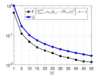
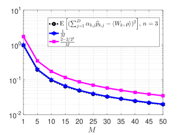
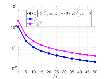
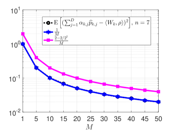
Figure 1: Numerical computation of $\operatorname{\mathbb{E}}[(\sum_{j=1}^{D}\alpha_{k,j}\cdot\widehat{p}_{k,j}-\langle\bm{W}_{k},\bm{\rho}\rangle)^{2}]$ for different $n$ and $M$.

3 Recovery Guarantee for Pauli Observable Measurements

In this section, we will study the recovery of a ground truth density matrix $\bm{\rho}^{\star}$ from the above-mentioned Pauli observable measurements.

3.1 Measurement setting and the matrix factorization approach

Definition 1 (Measurement setting).

Suppose we draw $\bm{A}_{1},\ldots,\bm{A}_{K}$ i.i.d. uniformly at random (with replacement) from the Pauli matrices $\{\bm{W}_{1},\ldots,\bm{W}_{D^{2}}\}$ defined in (5). We can generate $K$ Pauli observables for $\bm{\rho}^{\star}$ through the linear measurement operator $\mathcal{A}:\mathbb{C}^{D\times D}\rightarrow\mathbb{R}^{K}$ as

$$\bm{y}=\mathcal{A}(\bm{\rho}^{\star})=\begin{bmatrix}y_{1}\\ \vdots\\ y_{K}\end{bmatrix}=\begin{bmatrix}\langle\bm{A}_{1},\bm{\rho}^{\star}\rangle\\ \vdots\\ \langle\bm{A}_{K},\bm{\rho}^{\star}\rangle\end{bmatrix}=\begin{bmatrix}\sum_{j=1}^{D}\alpha_{1,j}\cdot p_{1,j}\\ \vdots\\ \sum_{j=1}^{D}\alpha_{K,j}\cdot p_{K,j}\end{bmatrix},$$ (16)

where $\{p_{k,1},\ldots,p_{k,D}\}$ are the Pauli basis measurements in (12). Note that $K$ also denotes the number of POVMs. For each $D$-outcome POVM, suppose we repeat the measurement process $M$ times and take the average of the outcomes to generate empirical probabilities

$$\widehat{p}_{k,j}=\frac{f_{k,j}}{M},\ k\in[K],\ j\in[D],$$ (17)

where $f_{k,j}$ denotes the number of times the $j$-th output is observed when using the $k$-th POVM $M$ times. We further denote the empirical Pauli observable measurements as

$$\widehat{\bm{y}}=\begin{bmatrix}\widehat{y}_{1}\\ \vdots\\ \widehat{y}_{K}\end{bmatrix}=\begin{bmatrix}\sum_{j=1}^{D}\alpha_{1,j}\cdot\widehat{p}_{1,j}\\ \vdots\\ \sum_{j=1}^{D}\alpha_{K,j}\cdot\widehat{p}_{K,j}\end{bmatrix}.$$ (18)

We denote by $\bm{e}$ the error in the empirical Pauli observable measurements:

$$\bm{e}=\widehat{\bm{y}}-\bm{y}\in\mathbb{R}^{K}.$$ (19)

Before introducing the loss function, it is helpful to incorporate a low-dimensional structure into the ground truth state $\bm{\rho}^{\star}$. The dimension of a quantum system grows exponentially with its components, such as the number of particles in the system. Consequently, the matrix size of $\bm{\rho}^{\star}$ becomes very large even for a moderately sized quantum system. To overcome challenges related to the direct estimation of the density matrix, such as computational and storage costs, we can exploit the inherent structure of pure or nearly pure quantum states characterized by low entropy and represented as low-rank density matrices [16, 13, 14, 15, 41]. However, dealing with the rank constraint in the density matrix often requires an expensive singular value decomposition (SVD), leading to high computational complexity. To address this, we propose a Burer-Monteiro type decomposition [42, 43] to represent the density matrix as follows:

$$\bm{\rho}=\bm{U}\bm{U}^{\rm H},\ \text{where}\ \bm{U}\in\mathbb{C}^{2^{n}\times r}\ \text{and}\ \|\bm{U}\|_{F}=1.$$ (20)

Based on this parameterization, we might consider a non-convex optimization problem as follows:

$$\operatorname*{\text{minimize}}_{\bm{U}\in\mathbb{C}^{2^{n}\times r}}f(\bm{U})=\frac{D}{2K}\bigg{\|}\mathcal{A}(\bm{U}\bm{U}^{\rm H})-\widehat{\bm{y}}\bigg{\|}_{2}^{2},$$ (21)

where $\mathcal{A}$ is the induced linear map as defined in (16).

We note, however, that as defined, $f(\bm{U})$ is non-holomorphic in the complex variable domain, rendering the computation and analysis of gradients and Hessians cumbersome. For this reason, we consider instead the problem

$$\operatorname*{\text{minimize}}_{\bm{U},\bm{U}^{*}\in\mathbb{C}^{D\times r}}f(\bm{U},\bm{U}^{*})=\frac{D}{2K}\bigg{\|}\mathcal{A}(\bm{U}{\bm{U}^{*}}^{\top})-\widehat{\bm{y}}\bigg{\|}_{2}^{2},$$ (22)

where $\bm{U}^{*}$, representing the complex conjugate of the matrix $\bm{U}$, is considered a second variable in the optimization. The benefit of parameterizing the objective function by both $\bm{U}$ and $\bm{U}^{*}$ is that $f(\bm{U},\bm{U}^{*})$ remains holomorphic in $\bm{U}$ for a fixed $\bm{U}^{*}$, and vice versa, allowing the use of Wirtinger derivatives to compute gradients and Hessians. While one could alternatively parameterize $f(\bm{U})$ by $\operatorname{Re}\left\{\bm{U}\right\}$ and $\operatorname{Im}\left\{\bm{U}\right\}$, this would increase the complexity of the analysis. We refer readers to [44, Chapter 3] for a comprehensive discussion on complex matrix analysis.

We also note that the solution set presented in (22) only comprises low-rank and PSD matrices, omitting the unit trace constraint. This omission arises because imposing the unit Frobenius norm does not notably diminish the magnitude of the recovery error. We refer readers to the additional discussions after Theorem 4 and Corollary 1. Thus, we will exclusively concentrate on the set of low-rank and PSD matrices without the unit trace constraint.

Despite $\ell_{2}$ loss being a convex function, the bilinear form in (20) renders the objective function of (22) nonconvex. This indicates that (22) may contain many saddle points or spurious local minima at which algorithms like Wirtinger gradient descent could get stuck. Therefore, it is crucial to conduct a thorough analysis of the landscape of (22) to better understand the distribution and characteristics of saddle points and local minima. Specifically, through the following analysis under the restricted isometry property (RIP) for Pauli observable measurements, we divide the objective function landscape into two regions. In one region, any critical points must be strict saddle points, at which algorithms like Wirtinger gradient descent will not get stuck. This implies that any local minima in (22) must reside in the other region. Then, by delving further into the information gleaned from the local minima, we explore the relationship between the total number of state copies $KM$ and recovery error.

Restricted isometry property with Pauli observable measurements

Our goal is to recover the low-rank density matrix $\bm{\rho}^{\star}$ from the underdetermined set of empirical Pauli observable measurements $\widehat{\bm{y}}$, where the number of coefficients $K$ is much smaller than the total number of entries in $\bm{\rho}^{\star}$, i.e., $K\ll D^{2}$. The key property necessary to achieve this is the restricted isometry property (RIP). The following results establish the RIP for $\mathcal{A}$ over low-rank matrices.

Theorem 2.

([12, Theorem 2.1]) Let the linear map $\mathcal{A}:\mathbb{C}^{D\times D}\rightarrow\mathbb{R}^{K}$ be defined in (16) and $0\leq\delta_{r}<1$. When the number of coefficients satisfies

$$K\geq C\cdot\frac{1}{\delta_{r}^{2}}Dr(\log D)^{6}$$ (23)

for some constant $C$, then, with overwhelming probability $1-e^{-C}$ over matrices $\bm{A}_{1},\ldots,\bm{A}_{K}$ selected i.i.d. uniformly from the set of Pauli matrices $\{\bm{W}_{1},\ldots,\bm{W}_{D^{2}}\}$, $\mathcal{A}$ satisfies the $(r,\delta_{r})$-RIP. That is, for all rank-$r$ $\bm{\rho}$, we have

$$(1-\delta_{r})\left\|\bm{\rho}\right\|_{F}^{2}\leq\frac{D}{K}\|\mathcal{A}(\bm{\rho})\|_{2}^{2}\leq(1+\delta_{r})\left\|\bm{\rho}\right\|_{F}^{2}.$$ (24)

In accordance with equation (24), when $\bm{\rho}$ has low rank, the RIP guarantees that the energy $\frac{D}{K}\|\mathcal{A}(\bm{\rho})\|_{2}^{2}$ is close to $\|\bm{\rho}\|_{F}^{2}$. The RIP can then be used to guarantee the recovery of $\bm{\rho}$ using only $O(Dr(\log D)^{6})$ Pauli observables. For example, for any two distinct low-rank Hermitian matrices $\bm{\rho}_{1},\bm{\rho}_{2}$ with rank $r$, the $(2r,\delta_{2r})$-RIP guarantees distinct measurements since

$$\frac{D}{K}\|\mathcal{A}(\bm{\rho}_{1})-\mathcal{A}(\bm{\rho}_{2})\|_{2}^{2}=\frac{D}{K}\|\mathcal{A}(\bm{\rho}_{1}-\bm{\rho}_{2})\|_{2}^{2}\geq(1-\delta_{2r})\|\bm{\rho}_{1}-\bm{\rho}_{2}\|_{F}^{2}.$$ (25)

3.2 Global landscape analysis

Before analyzing the recovery error, we need to characterize the locations of the critical points of $f(\bm{U},\bm{U}^{*})$. It is also necessary to characterize the second derivative behavior at these critical points. We commence by introducing the concepts of critical points, strict saddles, and the strict saddle property. Unlike in real matrix analysis, our consideration extends beyond $\bm{U}$ to also encompass $\bm{U}^{*}$ in the complex variable function, as $\bm{U}$ and $\bm{U}^{*}$ are regarded as two independent variables. For a comprehensive understanding of complex variable functions, please refer to [44, Chapters 3-4].

Definition 2.

(Critical points) We say $(\bm{U},\bm{U}^{*})$ is a critical point if the Wirtinger gradient at $(\bm{U},\bm{U}^{*})$ vanishes, i.e.,

$$\nabla f(\bm{U},\bm{U}^{*})=\begin{bmatrix}\nabla_{\bm{U}}f(\bm{U},\bm{U}^{*})\\ \nabla_{\bm{U}^{*}}f(\bm{U},\bm{U}^{*})\end{bmatrix}={\bm{0}}.$$ (26)

Note that $(\nabla_{\bm{U}}f(\bm{U},\bm{U}^{*}))^{*}=\nabla_{\bm{U}^{*}}f(\bm{U},\bm{U}^{*})$ always holds for a real-valued function $f(\bm{U},\bm{U}^{*})$.

Definition 3.

(Strict saddles) A critical point $(\bm{U},\bm{U}^{*})$ is a strict saddle if the Wirtinger Hessian matrix evaluated at this point has a strictly negative eigenvalue, i.e.,

$$\lambda_{\min}(\nabla^{2}f(\bm{U},\bm{U}^{*}))=\lambda_{\min}\bigg{(}\begin{bmatrix}\frac{\partial^{2}f(\bm{U},\bm{U}^{*})}{\partial{\text{vec}(\bm{U}^{*})}\partial{\text{vec}(\bm{U})^{\top}}}\frac{\partial^{2}f(\bm{U},\bm{U}^{*})}{\partial{\text{vec}(\bm{U}^{*})}\partial{\text{vec}(\bm{U}^{*})^{\top}}}\\ \frac{\partial^{2}f(\bm{U},\bm{U}^{*})}{\partial{\text{vec}(\bm{U})}\partial{\text{vec}(\bm{U})^{\top}}}\frac{\partial^{2}f(\bm{U},\bm{U}^{*})}{\partial{\text{vec}(\bm{U})}\partial{\text{vec}(\bm{U}^{*})^{\top}}}\end{bmatrix}\bigg{)}<0.$$ (27)

All other critical points that satisfy the second-order optimality condition, i.e., $\nabla^{2}f(\bm{U},\bm{U}^{*})\succeq 0$, are called second-order critical points.

Note that without distinguishing between local maxima and saddle points, we refer to a critical point as a strict saddle point only if its Wirtinger Hessian matrix has at least one strictly negative eigenvalue. Next, following the analysis in Appendix A, we formally establish the following theorem.

Theorem 3.

Suppose that $\bm{\rho}^{\star}\in\mathbb{C}^{D\times D}$ is a target density matrix of rank $r$ and linear map $\mathcal{A}$ satisfies the $(2r,\delta_{2r})$-RIP with $\delta_{2r}\leq 0.09$. Then any second-order critical point $(\bm{U},\bm{U}^{*})$ in the optimization problem (22) satisfies

$$\left\|\bm{U}\bm{U}^{\rm H}-\bm{\rho}^{\star}\right\|_{F}\leq D\sqrt{r}h(\delta_{2r})\frac{\|\mathcal{A}^{*}(\bm{e})\|}{K},$$ (28)

where $\bm{e}$ is defined in (19), $\mathcal{A}^{*}$ is the adjoint operator of $\mathcal{A}$ with $\mathcal{A}^{*}(\bm{e})=\sum_{k=1}^{K}e_{k}\bm{A}_{k}$, and $h(\delta_{2r})$ is defined as

$$h(\delta_{2r})=\frac{\sqrt{2}+\sqrt{82.55-762.54\delta_{2r}-843.09\delta_{2r}^{2}}}{1.5-15.7\delta_{2r}}.$$ (29)

In words, Theorem 3 implies that any critical point $(\bm{U},\bm{U}^{*})$ that is not close to the target solution, i.e., for which $\left\|\bm{U}\bm{U}^{\rm H}-\bm{\rho}^{\star}\right\|_{F}\geq D\sqrt{r}h(\delta_{2r})\frac{\|\mathcal{A}^{*}(\bm{e})\|}{K}$, must be a strict saddle point. As various iterative algorithms can escape strict saddles [45], this property ensures the convergence to a solution with the recovery guarantee in (28). The term $h(\delta_{2r})$ in the upper bound, as illustrated in Figure 2, is monotonically increasing with respect to $\delta_{2r}$, indicating that a smaller $\delta_{2r}$ could give a relatively better recovery as per (28). The term $\|\mathcal{A}^{*}(\bm{e})\|/K$ in (28) can be upper bounded by the following result.

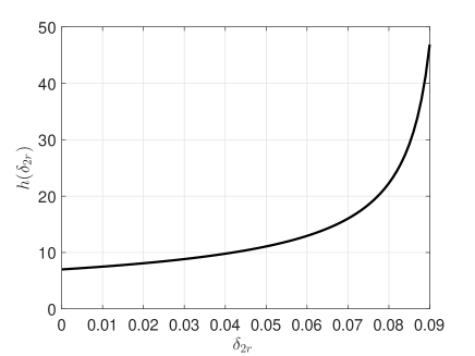
Figure 2: Plot of $h(\delta_{2r})$ in (29).

Lemma 2.

Assuming $M\leq O(K/n)$, then with probability at least $1-e^{-\Omega(n/(1+\sqrt{Mn/K}))}$, $\mathcal{A}$ in Definition 1 satisfies

$$\frac{\|\mathcal{A}^{*}(\bm{e})\|}{K}\lesssim\sqrt{\frac{\log D}{KM}}.$$ (30)

The proof is provided in Appendix B. Lemma 2 shows that the term $\|\mathcal{A}^{*}(\bm{e})\|/K$ caused by the statistical error in the empirical Pauli observable measurements depends only on the overall experimental resources $N=KM$, if ignoring the difference in the failure probability. This suggests that the recovery error remains comparable across various selections of $K$ and $M$, provided that $N=KM$ remains constant. However, we note that the probability of failure may increase significantly when $K$ is excessively small. The assumption $M\leq O(K/n)$ stems from a technical difficulty in applying the matrix Bernstein’s inequality, but we believe this assumption can be removed by more sophisticated analysis. By incorporating this result into Theorem 3, we can then obtain a recovery guarantee in terms of $K$ and $M$.

Theorem 4.

Under the Pauli observable setting in Definition 1, assume that $K\geq C\cdot\frac{1}{\delta_{2r}^{2}}Dr(\log D)^{6}$ for a positive constant $C$ such that $\mathcal{A}$ satisfies $(2r,\delta_{2r})$-RIP with constant $\delta_{2r}\leq 0.09$, as guaranteed by Theorem 2 with high probability. Supposing $M\leq O(K/n)$, then with probability at least $1-e^{-C/2}-e^{-\Omega(n/(1+\sqrt{Mn/K}))}$, any second-order critical point $(\bm{U},\bm{U}^{*})$ in the optimization problem (22) satisfies

$$\|\bm{U}\bm{U}^{\rm H}-\bm{\rho}^{\star}\|_{F}\lesssim h(\delta_{2r})\cdot\sqrt{\frac{D^{2}\log Dr}{KM}},$$ (31)

where $h(\delta_{2r})$ is defined in (29).

Quality versus quantity of Pauli observable measurements

When ignoring the term $h(\delta_{2r})$, the upper bound for the recovery error $\|\bm{U}\bm{U}^{\rm H}-\bm{\rho}^{\star}\|_{F}$ in (31) decays with the overall experimental resources $N=KM$. Specifically, a favorable scaling of $1/KM$ for the mean-squared error (i.e., $\|\bm{U}\bm{U}^{\rm H}-\bm{\rho}^{\star}\|_{F}^{2}$) is maintained for all sufficiently large $K$ such that the RIP is satisfied. On the other hand, the constant $\delta_{2r}$ decays with $K$ and $h(\delta_{2r})$ increases monotonically, albeit slowly, with $\delta_{2r}$ as depicted in Figure 2. From this perspective, for fixed total experimental resources $N$, using a larger value of $K$ generally results in a smaller recovery error bound. In particular, the extreme case with a single-sample measurement (i.e., $M=1$ and $K=N$), where each empirical Pauli observable measurement is extremely noisy, would give the best bound. This explains the successful application of single-sample measurements in recent work [17]. We will provide experiments in Section 5 to demonstrate the recovery performance for the different choices of $M$ and $K$.

For any $\epsilon>0$, (31) implies that $\|\bm{U}\bm{U}^{\rm H}-\bm{\rho}^{\star}\|_{F}\leq\epsilon$ when the number of state copies $KM\gtrsim D^{2}(\log D)r/\epsilon^{2}$. By using the inequality $\|\bm{U}\bm{U}^{\rm H}-\bm{\rho}^{\star}\|_{1}\leq\sqrt{2r}\left\|\bm{U}\bm{U}^{\rm H}-\bm{\rho}^{\star}\right\|_{F}$ since $\operatorname{rank}(\bm{U}\bm{U}^{\rm H}-\bm{\rho}^{\star})\leq 2r$, we can ensure $\epsilon$-accurate recovery in the trace distance with $\Omega(D^{2}(\log D)r^{2}/\epsilon^{2})$ state copies. When omitting the $\log D$ term, which might have been introduced for technical reasons, this sampling complexity is optimal for empirical Pauli observable measurements according to [19]. Finally, we note that while the solution $\bm{U}\bm{U}^{\rm H}$ of (22) may be non-physical as it may not have trace 1, we can easily obtain a physical state without compromising the recovery guarantee in Equation 31. Specifically, denoting by $\mathbb{S}_{+}:=\{\bm{\rho}\in\mathbb{C}^{2^{n}\times 2^{n}}:\bm{\rho}\succeq\bm{0},\operatorname{trace}(\bm{\rho})=1\}$ the set of physical states and $P_{\mathbb{S}_{+}}$ the projection onto the set $\mathbb{S}_{+}$ which can be efficiently computed by projecting the eigenvalues onto a simplex [46], we have

$$\|\mathcal{P}_{\mathbb{S}_{+}}(\bm{U}\bm{U}^{\rm H})-\bm{\rho}^{\star}\|_{F}\leq\|\bm{U}\bm{U}^{\rm H}-\bm{\rho}^{\star}\|_{F},$$ (32)

where the second inequality follows from the nonexpansiveness property of the convex set. This implies that the projection step ensures the state becomes physically valid while preserving or even improving the recovery guarantee.

4 Wirtinger Gradient Descent with Linear Convergence

Theorem 4 provides an upper bound on the recovery error for any second-order critical point of the least squares objective with empirical Pauli observable measurements. This result offers favorable guarantees for many iterative algorithms, including the computationally efficient gradient descent, which can almost surely converge to a second-order critical point [45]. However, this does not imply that gradient descent can efficiently find a second-order critical point. Indeed, gradient descent can be significantly slowed down by saddle points and may take exponential time to escape [47]. In this section, we study the optimization landscape near the target solution and show that the problem has a basin of attraction within which Wirtinger gradient descent has a fast convergence, with recovery error similar to (28).

In particular, with an appropriate initialization $\bm{U}_{0}$, we use the following Wirtinger gradient descent (GD):

$${\bm{U}}_{t}=\bm{U}_{t-1}-\mu\nabla_{\bm{U}^{*}}f(\bm{U}_{t-1},\bm{U}^{*}_{t-1}),$$ (33)

where $\mu$ is the step size. The complex conjugate part can also be updated as ${\bm{U}}_{t}^{*}=\bm{U}_{t-1}^{*}-\mu\nabla_{\bm{U}}f(\bm{U}_{t-1},\bm{U}^{*}_{t-1})$, which is exactly the same as taking the complex conjugate of (33) for the real-valued $f(\bm{U},\bm{U}^{*})$. Thus, one only needs to perform the gradient descent and study the performance for $\bm{U}_{t}$. To analyze the convergence, we need an appropriate metric to capture the distance between the factors $\bm{U}_{t}$ and the ground-truth factor $\bm{U}^{\star}$ that satisfies $\bm{\rho}^{\star}=\bm{U}^{\star}\bm{U}^{\star\mathrm{H}}$. Noting that for any unitary matrix $\bm{R}\in\mathcal{U}_{r}:=\{\bm{R}\in\mathbb{C}^{r\times r},\bm{R}^{\mathrm{H}}\bm{R}={\bf I}\}$, $\bm{U}^{\star}\bm{R}$ is also a factor of $\bm{\rho}^{\star}$ since $\bm{U}^{\star}\bm{R}\bm{R}^{\rm H}\bm{U}^{\star\rm H}=\bm{\rho}^{\star}$, we define the distance between any factor $\bm{U}$ and $\bm{U}^{\star}$ as [27]

$$\operatorname{dist}(\bm{U},\bm{U}^{\star})=\|\bm{U}-\bm{U}^{\star}\bm{R}\|_{F},\ \text{where}\ \bm{R}=\operatorname*{\text{arg~{}min}}_{\bm{R}^{\prime}\in\mathcal{U}_{r}}\|\bm{U}-\bm{U}^{\star}\bm{R}^{\prime}\|_{F}.$$ (34)

Based on the distance defined above, we can analyze the convergence of the Wirtinger GD by

$$\operatorname{dist}^{2}(\bm{U}_{t},\bm{U}^{\star}) \!\!\!\!=\!\!\!\! \|\bm{U}_{t}-\bm{U}^{\star}\bm{R}_{t}\|_{F}^{2}$$ (35)

$$\!\!\!\!\leq\!\!\!\! \|\bm{U}_{t-1}-\mu\nabla_{\bm{U}^{*}}f(\bm{U}_{t-1},\bm{U}_{t-1}^{*})-\bm{U}^{\star}\bm{R}_{t-1}\|_{F}^{2}$$

$$\!\!\!\!=\!\!\!\! \|\bm{U}_{t-1}-\bm{U}^{\star}\bm{R}_{t-1}\|_{F}^{2}+\mu^{2}\|\nabla_{\bm{U}^{*}}f(\bm{U}_{t-1},\bm{U}_{t-1}^{*})\|_{F}^{2}$$

$$-2\mu\operatorname{Re}\left\{\langle\bm{U}_{t-1}-\bm{U}^{\star}\bm{R}_{t-1},\nabla_{\bm{U}^{*}}f(\bm{U}_{t-1},\bm{U}_{t-1}^{*})\rangle\right\}.$$

To enable a sufficient decrease of the distance, the term $\operatorname{Re}\left\{\langle\bm{U}_{t-1}-\bm{U}^{\star}\bm{R}_{t-1},\nabla_{\bm{U}^{*}}f(\bm{U}_{t-1},\bm{U}_{t-1}^{*})\rangle\right\}$ needs to be sufficiently large, i.e., the search direction $-\nabla_{\bm{U}^{*}}f(\bm{U}_{t-1},\bm{U}_{t-1}^{*})$ needs to point towards to the target factor $\bm{U}^{\star}\bm{R}_{t-1}$, which can be guaranteed by strong convexity for convex functions. For real-valued matrix factorization problems, a regularity condition has been established to achieve that goal [27, Lemma 5.7]. Here, we extend the analysis to the complex domain.

Lemma 3.

(Regularity Condition) Under the Pauli observable setting in Definition 1, assume that $K\geq C\cdot\frac{1}{\delta_{3r}^{2}}Dr(\log D)^{6}$ for a positive constant $C$ such that $\mathcal{A}$ satisfies $(3r,\delta_{3r})$-RIP with constant $\delta_{3r}\leq 1/40$, as guaranteed by Theorem 2. Then, with probability at least $1-e^{-C/3}$, any $\bm{U}$ that is close to $\bm{U}^{\star}$ in the sense $\operatorname{dist}(\bm{U},\bm{U}^{\star})\leq\frac{\sigma_{r}(\bm{U}^{\star})}{4}$ satisfies

$$\operatorname{Re}\left\{\langle\nabla_{\bm{U}^{*}}f(\bm{U},\bm{U}^{*}),\bm{U}-\bm{U}^{\star}\bm{R}\rangle\right\}$$ (36)

$$\!\!\!\!\geq\!\!\!\! \frac{\sigma_{r}^{2}(\bm{U}^{\star})}{4}\|\bm{U}-\bm{U}^{\star}\bm{R}\|_{F}^{2}+\frac{2(1-4\delta_{3r})}{25(1+2\delta_{3r})^{2}}\|\nabla_{\bm{U}^{*}}f(\bm{U},\bm{U}^{*})\|_{F}^{2}-\frac{11D^{2}r}{K^{2}}\|\mathcal{A}^{*}(\bm{e})\|^{2}.$$

The proof is given in Appendix C. Towards interpreting the right hand side (RHS) of (36), first recall Lemma 2 and the subsequent discussion that the term $\|\mathcal{A}^{*}(\bm{e})\|/K$ decays with the overall experimental resources on the order of $1/\sqrt{KM}$. On the other hand, a larger $K$ can result in a smaller $\delta_{3r}$, and hence a larger $\frac{2(1-4\delta_{3r})}{25(1+2\delta_{3r})^{2}}$. This aligns with the observation in Theorem 4 that performance roughly depends on the entire experimental resources $KM$, but increasing $K$ can enhance performance. Note that the first two terms in the RHS of (36) decay as $\bm{U}$ approaches $\bm{U}^{\star}$, while the third term is constant for any $\bm{U}$. Thus, roughly speaking, the RHS is positive when $\bm{U}$ is relatively far from $\bm{U}^{\star}$, ensuring a sufficient decrease of one step of the Wirtinger GD update. However, it becomes negative when $\bm{U}$ is close to $\bm{U}^{\star}$, indicating that no further decrease can be ensured. Formally, plugging Lemma 3 into (35) gives

$$\|\bm{U}_{t}-\bm{U}^{\star}\bm{R}_{t}\|_{F}^{2} \!\!\!\!\leq\!\!\!\! \bigg{(}1-\frac{\sigma_{r}^{2}(\bm{U}^{\star})}{2}\mu\bigg{)}\|\bm{U}_{t-1}-\bm{U}^{\star}\bm{R}_{t-1}\|_{F}^{2}+\frac{22D^{2}r\mu}{K^{2}}\|\mathcal{A}^{*}(\bm{e})\|^{2}$$ (37)

$$\!\!\!\!\leq\!\!\!\! \bigg{(}1-\frac{\sigma_{r}^{2}(\bm{U}^{\star})}{2}\mu\bigg{)}^{t}\|\bm{U}_{0}-\bm{U}^{\star}\bm{R}_{0}\|_{F}^{2}+O\bigg{(}\frac{D^{2}(\log D)r}{\sigma_{r}^{2}(\bm{U}^{\star})KM}\bigg{)},$$

where the first inequality assumes $\mu\leq\frac{4(1-4\delta_{3r})}{25(1+2\delta_{3r})^{2}}$ and the second inequality uses Lemma 2. We summarize this local convergence property of Wirtinger GD in the following corollary.

Corollary 1.

(Local Convergence) Under the same setup as in Lemma 3, suppose the Wirtinger GD (33) starts with an initialization $\bm{U}_{0}$ that satisfies

$$\|\bm{U}_{0}-\bm{U}^{\star}\bm{R}_{0}\|_{F}\leq\frac{\sigma_{r}(\bm{U}^{\star})}{4}$$ (38)

and uses step size $\mu\leq\frac{4(1-4\delta_{3r})}{25(1+2\delta_{3r})^{2}}$. Then with probability at least $1-e^{-C/3}-e^{-\Omega(n/(1+\sqrt{Mn/K}))}$, we have

$$\|\bm{U}_{t}-\bm{U}^{\star}\bm{R}_{t}\|_{F}^{2}\leq\bigg{(}1-\frac{\sigma_{r}^{2}(\bm{U}^{\star})}{2}\mu\bigg{)}^{t}\|\bm{U}_{0}-\bm{U}^{\star}\bm{R}_{0}\|_{F}^{2}+O\bigg{(}\frac{D^{2}(\log D)r}{\sigma_{r}^{2}(\bm{U}^{\star})KM}\bigg{)}.$$ (39)

As above discussed, the first term in the RHS of (39) indicates that Wirtinger GD achieves a linear convergence rate in the first phase (when $\bm{U}_{t}$ has a large distance to the target), which is similar to the noiseless real-valued cases [27]. The second term in the RHS of (39), which dominates after a certain number of iterations, is consistent with the recovery guarantee in Theorem 4 except for the additional term $\sigma_{r}^{2}(\bm{U}^{\star})$ that only depends on the target state. Notice that based on the initialization condition $\|\bm{U}_{0}-\bm{U}^{\star}\bm{R}_{0}\|_{F}\leq\frac{\sigma_{r}(\bm{U}^{\star})}{4}$, we can obtain $\|\bm{U}_{t}\|\leq\|\bm{U}_{t}-\bm{U}^{\star}\bm{R}_{t}\|+\|\bm{U}^{\star}\bm{R}_{t}\|\leq\frac{5}{4}$ and further derive

$$\|\bm{\rho}_{t}-\bm{\rho}^{\star}\|_{F}^{2} \!\!\!\!=\!\!\!\! \|\bm{U}_{t}\bm{U}_{t}^{\rm H}-\bm{U}_{t}\bm{R}_{t}^{\rm H}{\bm{U}^{\star}}^{\rm H}+\bm{U}_{t}\bm{R}_{t}^{\rm H}{\bm{U}^{\star}}^{\rm H}-\bm{U}^{\star}{\bm{U}^{\star}}^{\rm H}\|_{F}^{2}$$ (40)

$$\!\!\!\!\leq\!\!\!\! (2\|\bm{U}_{t}\|+2\|\bm{U}^{\star}\|)\|\bm{U}_{t}-\bm{U}^{\star}\bm{R}_{t}\|_{F}^{2}\leq O\bigg{(}\frac{D^{2}(\log D)r}{\sigma_{r}^{2}(\bm{U}^{\star})KM}\bigg{)}.$$

Combing (32) and (40), we can conclude that the recovery error bound mentioned above is also applicable to the physical state.

Spectral initialization

To provide a good initialization that satisfies (38), we utilize the spectral initialization approach that has been widely used in the literature [38, 48, 29]. Specifically,

$$\bm{U}_{0}=\begin{bmatrix}(\lambda_{1})_{+}^{1/2}\bm{c}_{1}&\cdots&(\lambda_{r})_{+}^{1/2}\bm{c}_{r}\end{bmatrix},\quad\bm{C}\bm{\Lambda}\bm{C}^{\rm H}=\frac{D}{K}\sum_{k=1}^{K}\widehat{y}_{k}\bm{A}_{k},$$ (41)

where $(a)_{+}=\max(a,0)$, $\bm{c}_{i}$ denotes the $i$-th column of $\bm{C}$, and $\bm{C}\bm{\Lambda}\bm{C}^{\mathrm{H}}$ is the eigenvalue decomposition of $\frac{D}{K}\sum_{k=1}^{K}\widehat{y}_{k}\bm{A}_{k}$ with nonincreasing eigenvalues $\lambda_{1}\geq\cdots\geq\lambda_{D}$. The following result guarantees the performance of this initialization.

Theorem 5.

(Spectral Initialization) Under the same setup as in Lemma 3, assuming $M\lesssim K/n$, then with probability at least $1-e^{-C/3}-e^{-\Omega(n/(1+\sqrt{Mn/K}))}$, the spectral initialization (41) satisfies

$$\|\bm{U}_{0}-\bm{U}^{\star}\bm{R}_{0}\|_{F}^{2}\leq\frac{\bigg{(}4\delta_{3r}\|\bm{\rho}^{\star}\|_{F}+O\bigg{(}\sqrt{\frac{D^{2}(\log D)r}{KM}}\bigg{)}\bigg{)}^{2}}{2(\sqrt{2}-1)\sigma_{r}^{2}(\bm{U}^{\star})}.$$ (42)

The proof is provided in Appendix D. The RHS of (42) decays with $K$ and $M$, which can be chosen relatively large to ensure the spectral initialization satisfies the requirement in (38). We again observe a similar phenomenon in how $K$ and $M$ affect the RHS of (42): the first term $\delta_{3r}$ decays with $K$, while the second term $O(\sqrt{\frac{D^{2}(\log D)r}{KM}})$ only decreases with the total number of state copies.

5 Numerical Experiments

In this section, we present numerical experiments on quantum state tomography, focusing on low-rank density matrices, to demonstrate the applicability of our theoretical results. To begin, we randomly generate $K$ Pauli matrices and a rank-$r$ density matrix $\bm{\rho}^{\star}=\bm{U}^{\star}{\bm{U}^{\star}}^{\rm H}\in\mathbb{C}^{2^{n}\times 2^{n}}$, where $\bm{U}^{\star}=\frac{\bm{A}^{\star}+i\cdot\bm{B}^{\star}}{\|\bm{A}^{\star}+i\cdot\bm{B}^{\star}\|_{F}}\in\mathbb{C}^{2^{n}\times r}$ with the entries of $\bm{A}^{\star}$ and $\bm{B}^{\star}$ being drawn i.i.d. from the standard normal distribution. For all the following experiments, we simulate each over 20 Monte Carlo independent trials and compute the average over these 20 trials.

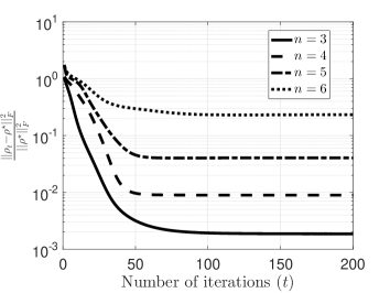
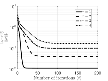
Figure 3: Performance comparison of Wirtinger GD, (a) for different $n$ with $r=2$, $\mu=0.3$, $K=2000$ and $M=100$, (b) for different $r$ with $n=5$, $\mu=0.3$, $K=2000$ and $M=100$.

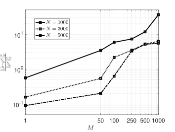
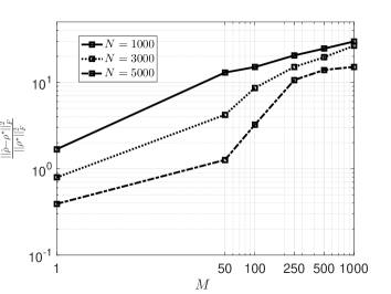
Figure 4: Performance comparison of Wirtinger GD for different $N$ and $M$ with (a) $n=4$, $r=1$, (b) $n=4$, $r=2$.

Convergence of Wirtinger GD

In the first set of experiments, we evaluate the performance of Wirtinger GD for various values of $n$ and $r$. Figures 3 and 3 illustrate the convergence behavior of the algorithm in minimizing the loss function defined in (22). We notice that as the values of $n$ or $r$ increase, the convergence rate of the Wirtinger GD decreases while recovery errors increase, which is aligned with the findings in 1.

Quality versus quantity of Pauli observable measurements

In the second set of experiments, we investigate the trade-off between the number of POVMs and the number of repeated measurements by choosing different $M$ when the total number of state copies $N=KM$ is fixed. To ensure convergence, we set step sizes $\mu=0.05$ for all the experiments. We plot the results for different choices of $r$ in Figures 4-4. As anticipated, when $N$ is fixed, overall we observe a reduction in the recovery error as $M$ decreases (or $K$ increases). This is because a larger $K$ produces more measurements and reduces the RIP constant of the measurement operator in (23), overcoming the issue of higher statistical error in the measurements. This finding corroborates the results presented in Theorem 4 and the practical use of single-sample measurements [17, 18].

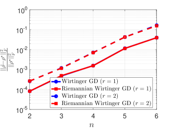
Figure 5: Performance comparison of different algorithms with $\mu=0.1$, $K=4000$ and $M=50$.

Incorporating sphere constraint

In the previous analysis, we have omitted the unit trace constraint for the factor in (20) because imposing the unit Frobenius norm does not notably improve the performance. To support this argument, in the third set of experiments, we compare the approaches with and without this constraint. Specifically, we impose the unit trace constraint on the factors $\{\bm{U}:\|\bm{U}\|_{F}=1\}$ in (22) and then employ the Riemannian Wirtinger GD to solve the corresponding problem, with updates

$$\widehat{\bm{U}}_{t}=\bm{U}_{t-1}-\mu\mathcal{P}_{T_{\bm{U}}\text{Sp}}(\nabla_{\bm{U}^{*}}f(\bm{U}_{t-1},\bm{U}^{*}_{t-1}))\ \ \text{and}\ \ {\bm{U}}_{t}=\frac{\widehat{\bm{U}}_{t}}{\|\widehat{\bm{U}}_{t}\|_{F}},$$ (43)

where $\mu$ is the step size and $\mathcal{P}_{T_{\bm{U}}\text{Sp}}(\bm{V})=\bm{V}-\langle\bm{U},\bm{V}\rangle\bm{U}$ denotes the projection onto the tangent space $T_{\bm{U}}\text{Sp}=\{\bm{Q}\in\mathbb{C}^{D\times r}:\langle\bm{U},\bm{Q}\rangle=0\}$, giving a Riemannian gradient. As shown in Figure 5, we observe that the two algorithms, Wirtinger GD and Riemannian Wirtinger GD, achieve on-par performance.

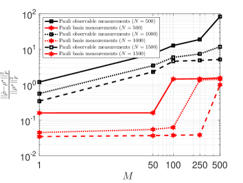
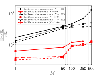
Figure 6: Performance comparison of the Wirtinger GD using empirical Pauli observable measurements and Pauli basis measurements with $\mu=1$ for different $N$, $M$ and (a) $n=4$, $r=1$, (b) $n=4$, $r=2$.

Directly using Pauli basis measurements for QST

Our work focused on the use of the expectation values of $n$-body Pauli observables in low-rank quantum state tomography to study the trade-off between the number of POVMs and the number of repeated measurements since the RIP with Pauli observables facilitates the analysis. Note that the Pauli observables are actually measured using the local Pauli basis, one could also recover the target state directly from the empirical probabilities of the Pauli basis measurement (see (14)).

Since Pauli basis measurements are also linear measurements of $\bm{\rho}^{\star}$, as described in (12), we can formulate a similar least squares minimization problem (22) and use the same Wirtinger GD to solve the problem. We conduct the numerical experiments under the same setting as the second set of experiments. By keeping the total number of measurements $N=KM$ constant, it becomes apparent that the Pauli basis measurements outperform Pauli observable measurements. One plausible explanation for this result is that the Pauli basis measurements involve $KD$ measurements, whereas the Pauli observable measurements involve only $K$ coefficients which are linear combinations of the Pauli basis measurements. On the other hand, with a fixed $N$, the recovery error associated with Pauli basis measurements also increases as $M$ grows. While we expect the analysis of the trade-off between the quality and quantity of measurements can be extended to Pauli basis measurements, one challenge is the lack of the RIP condition [12] for the Pauli basis measurements. We leave the investigation to future studies.

6 Conclusion

In this paper, we investigate the trade-off between the number of POVMs and the number of repeated measurements that control the quality of measurements for quantum state tomography, focusing on low-rank states and Pauli observable measurements for theoretical analysis. By exploiting the matrix factorization approach, we first study the global landscape of the factorized problem and show that every second-order critical point is a good estimator of the target state, with better recovery achieved by using a greater number of measurement settings, despite the large statistical error in each measurement. This finding suggests the advantage of using single-sample measurements when the total number of state copies is kept constant. Additionally, we prove that Wirtinger gradient descent converges locally at a linear rate. Numerical simulation results support our theoretical findings.

Appendix A Proof of Theorem 3

Proof.

Recall the objective $f(\bm{U},\bm{U}^{*})=\frac{D}{2K}\big{\|}\mathcal{A}(\bm{U}\bm{U}^{\rm H})-\widehat{\bm{y}}\big{\|}_{2}^{2}$ in (22). We first derive its Wirtinger gradient as follows:

$$\nabla f(\bm{U},\bm{U}^{*})=\begin{bmatrix}\nabla_{\bm{U}}f(\bm{U},\bm{U}^{*})\\ \nabla_{\bm{U}^{*}}f(\bm{U},\bm{U}^{*})\end{bmatrix}=\frac{D}{K}\sum_{k=1}^{K}\begin{bmatrix}(\langle\bm{A}_{k},\bm{U}\bm{U}^{\rm H}\rangle-\widehat{y}_{k})\bm{A}_{k}^{*}\bm{U}^{*}\\ (\langle\bm{A}_{k},\bm{U}\bm{U}^{\rm H}\rangle-\widehat{y}_{k})\bm{A}_{k}\bm{U}\end{bmatrix},$$ (44)

where we utilize the fact $\bm{A}_{k}=\bm{A}_{k}^{\rm H}$. It is noteworthy that within the framework of complex derivatives, the function $f(\bm{U})$ is written as $f(\bm{U},\bm{U}^{*})$ in the conjugate coordinates $(\bm{U},\bm{U}^{*})$. Therefore, we can independently compute the complex partial derivative $\nabla_{\bm{U}}f(\bm{U},\bm{U}^{*})$ and the complex conjugate partial derivative $\nabla_{\bm{U}^{*}}f(\bm{U},\bm{U}^{*})$, treating the complex variable $\bm{U}$ and its complex conjugate $\bm{U}^{*}$ as two independent variables.

Now we assume that $(\bm{U},\bm{U}^{*})$ is a critical point, i.e., $\nabla_{\bm{U}}f(\bm{U},\bm{U}^{*})={\bm{0}}$ and $\nabla_{\bm{U}^{*}}f(\bm{U},\bm{U}^{*})={\bm{0}}$. Let $\mathcal{P}_{\bm{U}}=\bm{U}^{{\rm H}\dagger}\bm{U}^{\rm H}$ be the orthogonal projection onto the range space of $\bm{U}$. Then, for any $\bm{Z}\in\mathbb{C}^{D\times r}$, we have

$$0 \!\!\!\!\!\!\!\!\!\!=\left\langle\nabla_{\bm{U}^{*}}f(\bm{U},\bm{U}^{*}),\bm{Z}\right\rangle=\frac{D}{K}\left\langle\mathcal{A}^{*}\mathcal{A}(\bm{U}\bm{U}^{\rm H}-\bm{\rho}^{\star}),\bm{Z}\bm{U}^{\rm H}\right\rangle-\frac{D}{K}\left\langle\mathcal{A}^{*}(\bm{e}),\bm{Z}\bm{U}^{\rm H}\right\rangle$$

$$\Longrightarrow \!\!\!\!\!\!\!\!\!\!\left\langle\bm{U}\bm{U}^{\rm H}-\bm{\rho}^{\star},\bm{Z}\bm{U}^{\rm H}\right\rangle=\left\langle\bm{U}\bm{U}^{\rm H}-\bm{\rho}^{\star},\bm{Z}\bm{U}^{\rm H}\right\rangle-\frac{D}{K}\left\langle\mathcal{A}^{*}\mathcal{A}(\bm{U}\bm{U}^{\rm H}-\bm{\rho}^{\star}),\bm{Z}\bm{U}^{\rm H}\right\rangle+\frac{D}{K}\left\langle\mathcal{A}^{*}(\bm{e}),\bm{Z}\bm{U}^{\rm H}\right\rangle$$

$$\Longrightarrow \!\!\!\!\!\!\!\!\!\!\left|\left\langle\bm{U}\bm{U}^{\rm H}-\bm{\rho}^{\star},\bm{Z}\bm{U}^{\rm H}\right\rangle\right|\leq 2\delta_{2r}\left\|\bm{U}\bm{U}^{\rm H}-\bm{\rho}^{\star}\right\|_{F}\left\|\bm{Z}\bm{U}^{\rm H}\right\|_{F}+\frac{D}{K}\left|\left\langle\mathcal{A}^{*}(\bm{e}),\bm{Z}\bm{U}^{\rm H}\right\rangle\right|$$

$$\Longrightarrow \!\!\!\!\!\!\!\!\!\!\left\|(\bm{U}\bm{U}^{\rm H}-\bm{\rho}^{\star})\mathcal{P}_{\bm{U}}\right\|_{F}^{2}\leq 2\delta_{2r}\left\|\bm{U}\bm{U}^{\rm H}-\bm{\rho}^{\star}\right\|_{F}\left\|(\bm{U}\bm{U}^{\rm H}-\bm{\rho}^{\star})\mathcal{P}_{\bm{U}}\right\|_{F}+\frac{D\sqrt{2r}}{K}\|\mathcal{A}^{*}(\bm{e})\|\left\|(\bm{U}\bm{U}^{\rm H}-\bm{\rho}^{\star})\mathcal{P}_{\bm{U}}\right\|_{F}$$

$$\Longrightarrow \!\!\!\!\!\!\!\!\!\!\left\|(\bm{U}\bm{U}^{\rm H}-\bm{\rho}^{\star})\mathcal{P}_{\bm{U}}\right\|_{F}\leq 2\delta_{2r}\left\|\bm{U}\bm{U}^{\rm H}-\bm{\rho}^{\star}\right\|_{F}+\frac{D\sqrt{2r}}{K}\|\mathcal{A}^{*}(\bm{e})\|,$$ (45)

where $\mathcal{A}^{*}$ is the adjoint operator of $\mathcal{A}$ and is defined as $\mathcal{A}^{*}({\bm{x}})=\sum_{k=1}^{K}x_{k}\bm{A}_{k}$ in the first equation, $\bm{e}$ is defined in (19), the first inequality follows Lemma 5, and the second inequality uses the substitutions $\bm{Z}=(\bm{U}\bm{U}^{\rm H}-\bm{\rho}^{\star})\bm{U}^{{\rm H}\dagger}$ and $\left|\left\langle\mathcal{A}^{*}(\bm{e}),\bm{Z}\bm{U}^{\rm H}\right\rangle\right|\leq\|\mathcal{A}^{*}(\bm{e})\|\left\|(\bm{U}\bm{U}^{\rm H}-\bm{\rho}^{\star})\mathcal{P}_{\bm{U}}\right\|_{*}\leq\sqrt{2r}\|\mathcal{A}^{*}(\bm{e})\|\left\|(\bm{U}\bm{U}^{\rm H}-\bm{\rho}^{\star})\mathcal{P}_{\bm{U}}\right\|_{F}$ according to the Von Neumann trace inequality.

To further characterize the locations of critical points, we need to leverage second derivative information to determine their signatures. By computing directional second derivatives, we can obtain the Wirtinger Hessian quadrature form for $\widetilde{\bm{\Delta}}=\begin{bmatrix}\bm{\Delta}\\ \bm{\Delta}^{*}\end{bmatrix}\in\mathbb{C}^{2D\times r}$ as follows:

$$\nabla^{2}f(\bm{U},\bm{U}^{*})[\widetilde{\bm{\Delta}},\widetilde{\bm{\Delta}}]$$ (46)

$$\!\!\!\!=\!\!\!\! \begin{bmatrix}(\text{vec}(\bm{\Delta}))^{\rm H}&(\text{vec}(\bm{\Delta}^{*}))^{\rm H}\end{bmatrix}\begin{bmatrix}\frac{\partial^{2}f(\bm{U},\bm{U}^{*})}{\partial{\text{vec}(\bm{U}^{*})}\partial{\text{vec}(\bm{U})^{\top}}}\frac{\partial^{2}f(\bm{U},\bm{U}^{*})}{\partial{\text{vec}(\bm{U}^{*})}\partial{\text{vec}(\bm{U}^{*})^{\top}}}\\ \frac{\partial^{2}f(\bm{U},\bm{U}^{*})}{\partial{\text{vec}(\bm{U})}\partial{\text{vec}(\bm{U})^{\top}}}\frac{\partial^{2}f(\bm{U},\bm{U}^{*})}{\partial{\text{vec}(\bm{U})}\partial{\text{vec}(\bm{U}^{*})^{\top}}}\end{bmatrix}\begin{bmatrix}\text{vec}(\bm{\Delta})\\ \text{vec}(\bm{\Delta}^{*})\end{bmatrix}$$

$$\!\!\!\!=\!\!\!\! \bigg{\langle}\bm{\Delta},\lim_{t\to 0}\frac{\nabla_{\bm{U}^{*}}f(\bm{U}+t\bm{\Delta},\bm{U}^{*})-\nabla_{\bm{U}^{*}}f(\bm{U},\bm{U}^{*})}{t}\bigg{\rangle}+\bigg{\langle}\bm{\Delta},\lim_{t\to 0}\frac{\nabla_{\bm{U}^{*}}f(\bm{U},\bm{U}^{*}+t\bm{\Delta}^{*})-\nabla_{\bm{U}^{*}}f(\bm{U},\bm{U}^{*})}{t}\bigg{\rangle}$$

$$+\bigg{\langle}\bm{\Delta}^{*},\lim_{t\to 0}\frac{\nabla_{\bm{U}}f(\bm{U}+t\bm{\Delta},\bm{U}^{*})-\nabla_{\bm{U}}f(\bm{U},\bm{U}^{*})}{t}\bigg{\rangle}+\bigg{\langle}\bm{\Delta}^{*},\lim_{t\to 0}\frac{\nabla_{\bm{U}}f(\bm{U},\bm{U}^{*}+t\bm{\Delta}^{*})-\nabla_{\bm{U}}f(\bm{U},\bm{U}^{*})}{t}\bigg{\rangle}$$

$$\!\!\!\!=\!\!\!\! \frac{2D}{K}\sum_{k=1}^{K}|\langle\bm{A}_{k},\bm{U}\bm{\Delta}^{\rm H}\rangle|^{2}+\frac{D}{K}\sum_{k=1}^{K}\langle\bm{A}_{k},\bm{U}\bm{\Delta}^{\rm H}\rangle\langle\bm{A}_{k},\bm{U}\bm{\Delta}^{\rm H}\rangle+\frac{D}{K}\sum_{k=1}^{K}\langle\bm{A}_{k},\bm{U}\bm{\Delta}^{\rm H}\rangle^{*}\langle\bm{A}_{k},\bm{U}\bm{\Delta}^{\rm H}\rangle^{*}$$

$$+\frac{2D}{K}\left\langle\mathcal{A}^{*}(\mathcal{A}(\bm{U}\bm{U}^{\rm H})-\widehat{\bm{y}}),\bm{\Delta}\bm{\Delta}^{\rm H}\right\rangle,$$

where we utilize $\bm{A}_{k}=\bm{A}_{k}^{\rm H}$ and $\langle\bm{A}_{k},\bm{U}\bm{\Delta}^{\rm H}\rangle=\langle\bm{A}_{k},\bm{\Delta}\bm{U}^{\rm H}\rangle^{*}$ in the last line.

With (A), the Wirtinger Hessian at any critical point $\bm{U}$ along the direction $\widetilde{\bm{\Delta}}=\bm{U}-\bm{U}^{\star}$ is given by

$$\nabla^{2}f(\bm{U},\bm{U}^{*})[\widetilde{\bm{\Delta}},\widetilde{\bm{\Delta}}]$$

$$\!\!\!\!\leq\!\!\!\! \frac{2D}{K}\left\langle\mathcal{A}^{*}(\mathcal{A}(\bm{U}\bm{U}^{\rm H})-\widehat{\bm{y}}),\bm{\Delta}\bm{\Delta}^{\rm H}\right\rangle+\frac{4D}{K}\|\mathcal{A}(\bm{U}\bm{\Delta}^{\rm H})\|_{2}^{2}$$

$$\!\!\!\!=\!\!\!\! \frac{2D}{K}\left\langle\mathcal{A}^{*}(\mathcal{A}(\bm{U}\bm{U}^{\rm H})-\widehat{\bm{y}}),(\bm{U}-\bm{U}^{\star})(\bm{U}-\bm{U}^{\star})^{\rm H}\right\rangle+\frac{4D}{K}\left\|\mathcal{A}(\bm{U}(\bm{U}-\bm{U}^{\star})^{\rm H})\right\|_{2}^{2}$$

$$\!\!\!\!=\!\!\!\! \frac{4D}{K}\left\|\mathcal{A}(\bm{U}(\bm{U}-\bm{U}^{\star})^{\rm H})\right\|_{2}^{2}-\frac{2D}{K}\left\langle\mathcal{A}^{*}(\mathcal{A}(\bm{U}\bm{U}^{\rm H})-\widehat{\bm{y}}),\bm{U}\bm{U}^{\rm H}-\bm{\rho}^{\star}\right\rangle$$

$$\!\!\!\!=\!\!\!\! \frac{4D}{K}\left\|\mathcal{A}(\bm{U}(\bm{U}-\bm{U}^{\star})^{\rm H})\right\|_{2}^{2}-\frac{2D}{K}\left\|\mathcal{A}(\bm{U}\bm{U}^{\rm H}-\bm{\rho}^{\star})\right\|_{2}^{2}+\frac{2D}{K}\left\langle\mathcal{A}^{*}(\bm{e}),\bm{U}\bm{U}^{\rm H}-\bm{\rho}^{\star}\right\rangle$$

$$\!\!\!\!\leq\!\!\!\! 4(1+\delta_{2r})\left\|\bm{U}(\bm{U}-\bm{U}^{\star})^{\rm H}\right\|_{F}^{2}-2(1-\delta_{2r})\left\|\bm{U}\bm{U}^{\rm H}-\bm{\rho}^{\star}\right\|_{F}^{2}+\frac{2\sqrt{2}D\sqrt{r}}{K}\|\mathcal{A}^{*}(\bm{e})\|\left\|\bm{U}\bm{U}^{\rm H}-\bm{\rho}^{\star}\right\|_{F}$$

$$\!\!\!\!\leq\!\!\!\! 4(1+\delta_{2r})\left(\frac{1}{8}\left\|\bm{U}\bm{U}^{\rm H}-\bm{\rho}^{\star}\right\|_{F}^{2}+\left(3+\frac{1}{2(\sqrt{2}-1)}\right)\left\|(\bm{U}\bm{U}^{\rm H}-\bm{\rho}^{\star})\mathcal{P}_{\bm{U}}\right\|_{F}^{2}\right)$$

$$-2(1-\delta_{2r})\left\|\bm{U}\bm{U}^{\rm H}-\bm{\rho}^{\star}\right\|_{F}^{2}+\frac{2\sqrt{2}D\sqrt{r}}{K}\|\mathcal{A}^{*}(\bm{e})\|\left\|\bm{U}\bm{U}^{\rm H}-\bm{\rho}^{\star}\right\|_{F}$$

$$\!\!\!\!\leq\!\!\!\! -\left(\frac{3}{2}-\frac{5}{2}\delta_{2r}-32(1+\delta_{2r})\delta_{2r}^{2}\left(3+\frac{1}{2(\sqrt{2}-1)}\right)\right)\left\|\bm{U}\bm{U}^{\rm H}-\bm{\rho}^{\star}\right\|_{F}^{2}$$

$$+\frac{16D^{2}r}{K^{2}}(1+\delta_{2r})\left(3+\frac{1}{2(\sqrt{2}-1)}\right)\|\mathcal{A}^{*}(\bm{e})\|^{2}+\frac{2\sqrt{2}D\sqrt{r}}{K}\|\mathcal{A}^{*}(\bm{e})\|\left\|\bm{U}\bm{U}^{\rm H}-\bm{\rho}^{\star}\right\|_{F}$$

$$\!\!\!\!\leq\!\!\!\! -(1.5-15.7\delta_{2r})\left\|\bm{U}\bm{U}^{\rm H}-\bm{\rho}^{\star}\right\|_{F}^{2}+\frac{53.7D^{2}r}{K^{2}}(1+\delta_{2r})\|\mathcal{A}^{*}(\bm{e})\|^{2}+\frac{2\sqrt{2}D\sqrt{r}}{K}\|\mathcal{A}^{*}(\bm{e})\|\left\|\bm{U}\bm{U}^{\rm H}-\bm{\rho}^{\star}\right\|_{F},$$

where the first inequality follows $\langle\bm{A}_{k},\bm{U}\bm{\Delta}^{\rm H}\rangle\langle\bm{A}_{k},\bm{U}\bm{\Delta}^{\rm H}\rangle+\langle\bm{A}_{k},\bm{U}\bm{\Delta}^{\rm H}\rangle^{*}\langle\bm{A}_{k},\bm{U}\bm{\Delta}^{\rm H}\rangle^{*}\leq 2|\langle\bm{A}_{k},\bm{U}\bm{\Delta}^{\rm H}\rangle|^{2}$, the second equality utilizes the first-order optimality condition $\nabla_{\bm{U}^{*}}f(\bm{U},\bm{U}^{*})=0$, the second inequality applies Equation 23, the third inequality uses Lemma 7, the fourth inequality uses (A), and the last line uses the assumption $\delta_{2r}\leq 0.09$.

Now the right hand side of (A) is negative when

$$\left\|\bm{U}\bm{U}^{\rm H}-\bm{\rho}^{\star}\right\|_{F}\geq\underbrace{\frac{\sqrt{2}+\sqrt{82.55-762.54\delta_{2r}-843.09\delta_{2r}^{2}}}{1.5-15.7\delta_{2r}}}_{h(\delta_{2r})}\frac{D\sqrt{r}}{K}\|\mathcal{A}^{*}(\bm{e})\|,$$ (48)

ensuring that $\lambda_{\min}(\nabla^{2}f(\bm{U},\bm{U}^{*}))<0$ and hence these critical points are strict saddle points.

In other words, when both the first- and second-order optimality conditions are satisfied at $\bm{U}$, the Wirtinger Hessian matrix is PSD and the right hand side of (A) is non-negative, implying that $\bm{U}$ satisfies

$$\left\|\bm{U}\bm{U}^{\rm H}-\bm{\rho}^{\star}\right\|_{F}\leq h(\delta_{2r})\frac{D\sqrt{r}}{K}\|\mathcal{A}^{*}(\bm{e})\|.$$ (49)

∎

Appendix B Proof of Lemma 2

Proof.

To bound

$$\|\mathcal{A}^{*}(\bm{e})\|=\bigg{\|}\sum_{k=1}^{K}e_{k}\bm{A}_{k}\bigg{\|}=\bigg{\|}\sum_{k=1}^{K}\left(\sum_{j=1}^{D}\alpha_{k,j}\widehat{p}_{k,j}-\left\langle\bm{A}_{k},\bm{\rho}^{\star}\right\rangle\right)\bm{A}_{k}\bigg{\|},$$ (50)

we first utilize $\operatorname{\mathbb{E}}[f_{k,j}]=Mp_{k,j}$ to get

$$\operatorname{\mathbb{E}}\bigg{[}{\bigg{(}\sum_{j=1}^{D}\alpha_{k,j}\widehat{p}_{k,j}-\left\langle\bm{A}_{k},\bm{\rho}^{\star}\right\rangle\bigg{)}\bm{A}_{k}}\bigg{]}$$ (51)

$$\!\!\!\!=\!\!\!\! \operatorname{\mathbb{E}}_{f_{k,j}}\bigg{[}{\bigg{(}\sum_{j=1}^{D}\alpha_{k,j}\frac{f_{k,j}}{M}-\sum_{j=1}^{D}\alpha_{k,j}p_{k,j}\bigg{)}\bm{A}_{k}}\bigg{|}\bm{A}_{k}\bigg{]}\operatorname{\mathbb{E}}[\bm{A}_{k}]={\bm{0}}.$$

It follows from $\|\bm{A}_{k}\|=1$ and $\left|\sum_{j=1}^{D}\alpha_{k,j}\widehat{p}_{k,j}-\left\langle\bm{A}_{k},\bm{\rho}^{\star}\right\rangle\right|\leq 2$ that

$$\bigg{\|}\bigg{(}\sum_{j=1}^{D}\alpha_{k,j}\widehat{p}_{k,j}-\left\langle\bm{A}_{k},\bm{\rho}^{\star}\right\rangle\bigg{)}\bm{A}_{k}\bigg{\|}\leq 2.$$ (52)

Moreover, with $\operatorname{\mathbb{E}}[\bm{A}_{k}^{2}]={\bf I}_{D}$ and $\operatorname{\mathbb{E}}\left[\left(\sum_{j=1}^{D}\alpha_{k,j}\widehat{p}_{k,j}-\left\langle\bm{A}_{k},\bm{\rho}^{\star}\right\rangle\right)^{2}\right]\leq\frac{2}{M}$ which follows Lemma 4, we have

$$\bigg{\|}\sum_{k=1}^{K}\operatorname{\mathbb{E}}\left[\left(\left(\sum_{j=1}^{D}\alpha_{k,j}\widehat{p}_{k,j}-\left\langle\bm{A}_{k},\bm{\rho}^{\star}\right\rangle\right)\bm{A}_{k}\right)^{2}\right]\bigg{\|}$$ (53)

$$\!\!\!\!\leq\!\!\!\! \sum_{k=1}^{K}\operatorname{\mathbb{E}}_{\widehat{p}_{k,j}}\bigg{[}\left(\sum_{j=1}^{D}\alpha_{k,j}\widehat{p}_{k,j}-\left\langle\bm{A}_{k},\bm{\rho}^{\star}\right\rangle\right)^{2}\bigg{|}\bm{A}_{k}\bigg{]}\|\operatorname{\mathbb{E}}[\bm{A}_{k}^{2}]\|\leq\frac{2K}{M}.$$

Now, plugging (51), (52) and (53) into the matrix Bernstein’s inequality in Lemma 8 gives that

$$\operatorname{\mathbb{P}}\left(\bigg{\|}\sum_{k=1}^{K}\left(\sum_{j=1}^{D}\alpha_{k,j}\widehat{p}_{k,j}-\left\langle\bm{A}_{k},\bm{\rho}^{\star}\right\rangle\right)\bm{A}_{k}\bigg{\|}\geq t\right)\leq D\exp\left(\frac{-t^{2}}{4K/M+\frac{4}{3}t}\right).$$ (54)

Using $t=c\sqrt{K\log D/M}$ with a constant $c$ and $M\leq O(\frac{K}{n})$ in the above inequality leads to

$$\operatorname{\mathbb{P}}\left(\|\mathcal{A}^{*}(\bm{e})\|\geq c\sqrt{K\log D/M}\right)$$ (55)

$$\!\!\!\!=\!\!\!\! \operatorname{\mathbb{P}}\left(\bigg{\|}\sum_{k=1}^{K}\left(\sum_{j=1}^{D}\alpha_{k,j}\widehat{p}_{k,j}-\left\langle\bm{A}_{k},\bm{\rho}^{\star}\right\rangle\right)\bm{A}_{k}\bigg{\|}\geq c\sqrt{K\log D/M}\right)$$

$$\!\!\!\!\leq\!\!\!\! D\exp\left(\frac{-c^{2}\log D}{4+\frac{4}{3}c\sqrt{\frac{M\log D}{K}}}\right).$$

Hence, we have $\|\mathcal{A}^{*}(\bm{e})\|\leq c\sqrt{K\log D/M}$ with probability $1-e^{-\Omega(n/(1+\sqrt{Mn/K}))}$. ∎

Appendix C Proof of Lemma 3

Proof.

We first define one loss function $F(\bm{U},\bm{U}^{*})=\frac{1}{2}\|\bm{U}\bm{U}^{\rm H}-\bm{U}^{\star}{\bm{U}^{\star}}^{\rm H}\|_{F}^{2}$. Then we analyze

$$\operatorname{Re}\left\{\bigg{\langle}\nabla_{\bm{U}^{*}}F(\bm{U},\bm{U}^{*})-\nabla_{\bm{U}^{*}}f(\bm{U},\bm{U}^{*}),\bm{U}-\bm{U}^{\star}\bm{R}\bigg{\rangle}\right\}$$ (56)

$$\!\!\!\!=\!\!\!\! \operatorname{Re}\left\{\bigg{\langle}(\bm{U}\bm{U}^{\rm H}-\bm{U}^{\star}{\bm{U}^{\star}}^{\rm H})\bm{U}-\frac{D}{K}\sum_{k=1}^{K}\langle\bm{A}_{k},\bm{U}\bm{U}^{\rm H}-\bm{U}^{\star}{\bm{U}^{\star}}^{\rm H}\rangle\bm{A}_{k}\bm{U}+\frac{D}{K}\sum_{k=1}^{K}e_{k}\bm{A}_{k}\bm{U},\bm{U}-\bm{U}^{\star}\bm{R}\bigg{\rangle}\right\}$$

$$\!\!\!\!=\!\!\!\! \operatorname{Re}\left\{\langle(\bm{U}\bm{U}^{\rm H}-\bm{U}^{\star}{\bm{U}^{\star}}^{\rm H}),(\bm{U}-\bm{U}^{\star}\bm{R})\bm{U}^{\rm H}\rangle\right\}-\frac{D}{K}\operatorname{Re}\left\{\langle\mathcal{A}(\bm{U}\bm{U}^{\rm H}-\bm{U}^{\star}{\bm{U}^{\star}}^{\rm H}),\mathcal{A}((\bm{U}-\bm{U}^{\star}\bm{R})\bm{U}^{\rm H})\rangle\right\}$$

$$+\operatorname{Re}\left\{\bigg{\langle}\frac{D}{K}\sum_{k=1}^{K}e_{k}\bm{A}_{k},(\bm{U}-\bm{U}^{\star}\bm{R})\bm{U}^{\rm H}\bigg{\rangle}\right\}$$

$$\!\!\!\!\leq\!\!\!\! 2\delta_{3r}\|\bm{U}\bm{U}^{\rm H}-\bm{U}^{\star}{\bm{U}^{\star}}^{\rm H}\|_{F}\|(\bm{U}-\bm{U}^{\star}\bm{R})\bm{U}^{\rm H}\|_{F}+\frac{D\sqrt{r}}{K}\|(\bm{U}-\bm{U}^{\star}\bm{R})\bm{U}^{\rm H}\|_{F}\|\mathcal{A}^{*}(\bm{e})\|$$

$$\!\!\!\!=\!\!\!\! \delta_{3r}\|\bm{U}\bm{U}^{\rm H}-\bm{U}^{\star}{\bm{U}^{\star}}^{\rm H}\|_{F}^{2}+(\frac{1}{40}+\delta_{3r})\|(\bm{U}-\bm{U}^{\star}\bm{R})\bm{U}^{\rm H}\|_{F}^{2}+\frac{10D^{2}r}{K^{2}}\|\mathcal{A}^{*}(\bm{e})\|^{2},$$

where the first inequality uses Lemma 5 and $\langle\sum_{k=1}^{K}e_{k}\bm{A}_{k}\bm{U},\bm{U}-\bm{U}^{\star}\bm{R}\rangle\leq\|\mathcal{A}^{*}(\bm{e})\|\|(\bm{U}-\bm{U}^{\star}\bm{R})\bm{U}^{\rm H}\|_{*}\leq\sqrt{r}\|(\bm{U}-\bm{U}^{\star}\bm{R})\bm{U}^{\rm H}\|_{F}\|\mathcal{A}^{*}(\bm{e})\|$ based on the Von Neumann trace inequality.

Moreover, we can also derive

$$\|\nabla_{\bm{U}^{*}}f(\bm{U},\bm{U}^{*})\|_{F}-\|\nabla_{\bm{U}^{*}}F(\bm{U},\bm{U}^{*})\|_{F}$$ (57)

$$\!\!\!\!\leq\!\!\!\! \|\nabla_{\bm{U}^{*}}f(\bm{U},\bm{U}^{*})-\nabla_{\bm{U}^{*}}F(\bm{U},\bm{U}^{*})\|_{F}$$

$$\!\!\!\!=\!\!\!\! \bigg{\|}\frac{D}{K}\sum_{k=1}^{K}\langle\bm{A}_{k},\bm{U}\bm{U}^{\rm H}-\bm{U}^{\star}{\bm{U}^{\star}}^{\rm H}\rangle\bm{A}_{k}\bm{U}-\frac{D}{K}\sum_{k=1}^{K}e_{k}\bm{A}_{k}\bm{U}-(\bm{U}\bm{U}^{\rm H}-\bm{U}^{\star}{\bm{U}^{\star}}^{\rm H})\bm{U}\bigg{\|}_{F}$$

$$\!\!\!\!\leq\!\!\!\! \bigg{\|}\frac{D}{K}\sum_{k=1}^{K}\langle\bm{A}_{k},\bm{U}\bm{U}^{\rm H}-\bm{U}^{\star}{\bm{U}^{\star}}^{\rm H}\rangle\bm{A}_{k}\bm{U}-(\bm{U}\bm{U}^{\rm H}-\bm{U}^{\star}{\bm{U}^{\star}}^{\rm H})\bm{U}\bigg{\|}_{F}+\bigg{\|}\frac{D}{K}\sum_{k=1}^{K}e_{k}\bm{A}_{k}\bm{U}\bigg{\|}_{F}$$

$$\!\!\!\!\leq\!\!\!\! \frac{5\delta_{3r}}{2}\|\bm{U}\bm{U}^{\rm H}-\bm{U}^{\star}{\bm{U}^{\star}}^{\rm H}\|_{F}+\frac{5D}{4K}\|\mathcal{A}^{*}(\bm{e})\|,$$

where the last line follows Lemma 5 and $\|\bm{U}\|_{F}\leq\frac{5}{4}$ due to $\|\bm{U}-\bm{U}^{\star}\bm{R}\|_{F}\leq\frac{\sigma_{r}(\bm{U}^{\star})}{4}$ and $\|\bm{U}^{\star}\|_{F}=1$.

Considering that $\|\nabla_{\bm{U}^{*}}F(\bm{U},\bm{U}^{*})\|_{F}\leq\frac{5}{4}\|\bm{U}\bm{U}^{\rm H}-\bm{U}^{\star}{\bm{U}^{\star}}^{\rm H}\|_{F}$, we have

$$\|\nabla_{\bm{U}^{*}}f(\bm{U},\bm{U}^{*})\|_{F}^{2}\leq\frac{25}{8}(1+2\delta_{3r})^{2}\|\bm{U}\bm{U}^{\rm H}-\bm{U}^{\star}{\bm{U}^{\star}}^{\rm H}\|_{F}^{2}+\frac{25D^{2}}{8K^{2}}\|\mathcal{A}^{*}(\bm{e})\|^{2}.$$ (58)

Combining Lemma 9 and (56), we finally have

$$\operatorname{Re}\left\{\langle\nabla_{\bm{U}^{*}}f(\bm{U},\bm{U}^{*}),\bm{U}-\bm{U}^{\star}\bm{R}\rangle\right\}$$ (59)

$$\!\!\!\!=\!\!\!\! \operatorname{Re}\left\{\langle\nabla_{\bm{U}^{*}}f(\bm{U},\bm{U}^{*})-\nabla_{\bm{U}^{*}}F(\bm{U},\bm{U}^{*}),\bm{U}-\bm{U}^{\star}\bm{R}\rangle\right\}+\operatorname{Re}\left\{\langle\nabla_{\bm{U}^{*}}F(\bm{U},\bm{U}^{*}),\bm{U}-\bm{U}^{\star}\bm{R}\rangle\right\}$$

$$\!\!\!\!\geq\!\!\!\! -\delta_{3r}\|\bm{U}\bm{U}^{\rm H}-\bm{U}^{\star}{\bm{U}^{\star}}^{\rm H}\|_{F}^{2}-\bigg{(}\frac{1}{40}+\delta_{3r}\bigg{)}\|(\bm{U}-\bm{U}^{\star}\bm{R})\bm{U}^{\rm H}\|_{F}^{2}-\frac{10D^{2}r}{K^{2}}\|\mathcal{A}^{*}(\bm{e})\|^{2}$$

$$+\frac{1}{4}\|\bm{U}\bm{U}^{\rm H}-\bm{U}^{\star}{\bm{U}^{\star}}^{\rm H}\|_{F}^{2}+\frac{1}{20}\|(\bm{U}-\bm{U}^{\star}\bm{R})\bm{U}^{\rm H}\|_{F}^{2}+\frac{\sigma_{r}^{2}(\bm{U}^{\star})}{4}\|\bm{U}-\bm{U}^{\star}\bm{R}\|_{F}^{2}$$

$$\!\!\!\!\geq\!\!\!\! \bigg{(}\frac{1}{4}-\delta_{3r}\bigg{)}\|\bm{U}\bm{U}^{\rm H}-\bm{U}^{\star}{\bm{U}^{\star}}^{\rm H}\|_{F}^{2}+\frac{\sigma_{r}^{2}(\bm{U}^{\star})}{4}\|\bm{U}-\bm{U}^{\star}\bm{R}\|_{F}^{2}-\frac{10D^{2}r}{K^{2}}\|\mathcal{A}^{*}(\bm{e})\|^{2}$$

$$\!\!\!\!\geq\!\!\!\! \frac{\sigma_{r}^{2}(\bm{U}^{\star})}{4}\|\bm{U}-\bm{U}^{\star}\bm{R}\|_{F}^{2}+\frac{2(1-4\delta_{3r})}{25(1+2\delta_{3r})^{2}}\|\nabla_{\bm{U}^{*}}f(\bm{U},\bm{U}^{*})\|_{F}^{2}-\frac{11D^{2}r}{K^{2}}\|\mathcal{A}^{*}(\bm{e})\|^{2},$$

where the second and last inequalities respectively follow $\delta_{3r}\leq\frac{1}{40}$ and (58).

∎

Appendix D Proof of Theorem 5

Proof.

Following [49], we begin by introducing the restricted Frobenius norm, defined as

$$\|\bm{X}\|_{F,r}=\max_{\bm{Y}\in\mathbb{C}^{m\times n},\ \|\bm{Y}\|_{F}\leq 1,\atop\text{rank}(\bm{Y})=r}|\langle\bm{X},\bm{Y}\rangle|$$ (60)

for any $\bm{X}\in\mathbb{C}^{m\times n}$. Next, we analyze

$$\|\bm{\rho}_{0}-\bm{\rho}^{\star}\|_{F} \!\!\!\!=\!\!\!\! \|\bm{U}_{0}\bm{U}_{0}^{\rm H}-\bm{\rho}^{\star}\|_{F,2r}$$ (61)

$$\!\!\!\!\leq\!\!\!\! 2\bigg{\|}\frac{D}{K}\sum_{k=1}^{K}\widehat{y}_{k}\bm{A}_{k}-\bm{\rho}^{\star}\bigg{\|}_{F,2r}$$

$$\!\!\!\!\leq\!\!\!\! 2\bigg{\|}\frac{D}{K}\mathcal{A}^{*}(\mathcal{A}(\bm{\rho}^{\star}))-\bm{\rho}^{\star}\bigg{\|}_{F,2r}+\frac{2D}{K}\|\mathcal{A}^{*}(\bm{e})\|_{2r}$$

$$\!\!\!\!\leq\!\!\!\! 2\max_{\bm{Y}\in\mathbb{C}^{D\times D},\ \|\bm{Y}\|_{F}\leq 1,\atop\text{rank}(\bm{Y})=2r}\bigg{\langle}\bigg{(}\frac{D}{K}\mathcal{A}^{*}\mathcal{A}-\mathcal{I}\bigg{)}(\bm{\rho}^{\star}),\bm{Y}\bigg{\rangle}+\frac{2D\sqrt{2r}}{K}\|\mathcal{A}^{*}(\bm{e})\|$$

$$\!\!\!\!\leq\!\!\!\! 4\delta_{3r}\|\bm{\rho}^{\star}\|_{F}+O\bigg{(}\sqrt{\frac{D^{2}(\log D)r}{KM}}\bigg{)},$$

where the first inequality follows from the quasi-optimality property of truncated eigenvalue decomposition projection [50] and the last line uses Lemma 5 and Lemma 2 which are simultaneously satisfied with probability $1-e^{-C/3}-e^{-\Omega(n/(1+\sqrt{Mn/K}))}$.

Furthermore, based on Lemma 10, we can obtain

$$\|\bm{U}_{0}-\bm{U}^{\star}\bm{R}_{0}\|_{F}^{2} \!\!\!\!\leq\!\!\!\! \frac{1}{2(\sqrt{2}-1)\sigma_{r}^{2}(\bm{U}^{\star})}\|\bm{\rho}_{0}-\bm{\rho}^{\star}\|_{F}^{2}$$ (62)

$$\!\!\!\!\leq\!\!\!\! \frac{\bigg{(}4\delta_{3r}\|\bm{\rho}^{\star}\|_{F}+O\bigg{(}\sqrt{\frac{D^{2}(\log D)r}{KM}}\bigg{)}\bigg{)}^{2}}{2(\sqrt{2}-1)\sigma_{r}^{2}(\bm{U}^{\star})},$$

where $\bm{R}_{0}=\operatorname*{\text{arg~{}min}}_{\bm{R}^{\prime}\in\mathcal{U}_{r}}\|\bm{U}_{0}-\bm{U}^{\star}\bm{R}^{\prime}\|_{F}$.

∎

Appendix E Auxiliary Materials

Lemma 4.

Given a set of probabilities $(p_{1},\dots,p_{D})$, we can generate empirical probabilities $\widehat{p}_{q}=\frac{\#\text{ of $q$-th output}}{M},\ \forall q\in[D]:=\{1,\ldots,D\}$ by repeating the measurement process $M$ times and taking the average of the outcomes. So $(\widehat{p}_{1},\dots,\widehat{p}_{D})$ follows the multinomial distribution $\operatorname{Multinomial}(M,\bm{p})$ with the covariance matrix $\bm{\Sigma}$. Elements of $\bm{\Sigma}$ are $\Sigma_{i,k}=\begin{cases}\frac{p_{i}(1-p_{i})}{M},&i=k,\\ -\frac{p_{i}p_{k}}{M},&i\neq k.\end{cases}$. Then

$$\operatorname{\mathbb{E}}\left(\sum_{q=1}^{D}\alpha_{q}\left(\widehat{p}_{q}-p_{q}\right)\right)^{2}\leq\frac{2-1/D}{M}$$ (63)

holds for any $\alpha_{q}=\pm 1,q=1,\ldots,D$.

Proof.

Based on the covariance matrix of the multinomial distribution, we have

$$\operatorname{\mathbb{E}}\left[(\widehat{p}_{q}-p_{q})(\widehat{p}_{q^{\prime}}-p_{q^{\prime}})\right]=\begin{cases}-\frac{1}{M}p_{q}p_{q^{\prime}},&q\neq q^{\prime},\\ \frac{1}{M}p_{q}(1-p_{q}),&q=q^{\prime},\end{cases}$$ (64)

and further derive

$$\operatorname{\mathbb{E}}\left(\sum_{q=1}^{D}\alpha_{j}\left(\widehat{p}_{q}-p_{q}\right)\right)^{2} \!\!\!\!=\!\!\!\! \sum_{q=1}^{D}\sum_{q^{\prime}=1}^{D}\alpha_{q}\alpha_{q^{\prime}}\operatorname{\mathbb{E}}\left[\left(\widehat{p}_{q}-p_{q}\right)\left(\widehat{p}_{q^{\prime}}-p_{q^{\prime}}\right)\right]$$ (65)

$$\!\!\!\!\leq\!\!\!\! \sum_{q=1}^{D}\sum_{q^{\prime}=1}^{D}\left|\operatorname{\mathbb{E}}\left[\left(\widehat{p}_{q}-p_{q}\right)\left(\widehat{p}_{q^{\prime}}-p_{q^{\prime}}\right)\right]\right|$$

$$\!\!\!\!=\!\!\!\! \sum_{q\neq q^{\prime}}\frac{1}{M}p_{q}p_{q^{\prime}}+\sum_{q=1}^{D}\frac{1}{M}p_{q}(1-p_{q})$$

$$\!\!\!\!\leq\!\!\!\! \frac{2-2/D}{M},$$

where the last inequality follows $\sum_{q\neq q^{\prime}}p_{q}p_{q^{\prime}}-\sum_{q=1}^{D}p_{q}^{2}=1-2\sum_{q=1}^{D}p_{q}^{2}\leq 1-\frac{2}{D}$ and $\sum_{q=1}^{D}p_{q}=1$.

∎

Lemma 5.

Suppose that $\mathcal{A}$ obeys the $(2r,\delta_{2r})$-RIP in Theorem 2. Then for any $\bm{\rho}_{1},\bm{\rho}_{2}\in\mathbb{C}^{D\times D}$ of rank at most $r$, one has

$$\bigg{|}\frac{D}{K}\langle\mathcal{A}(\bm{\rho}_{1}),\mathcal{A}(\bm{\rho}_{2})\rangle-\langle\bm{\rho}_{1},\bm{\rho}_{2}\rangle\bigg{|}\leq 2\delta_{2r}\|\bm{\rho}_{1}\|_{F}\|\bm{\rho}_{2}\|_{F},$$ (66)

or equivalently,

$$\bigg{|}\bigg{\langle}\bigg{(}\frac{D}{K}\mathcal{A}^{*}\mathcal{A}-\mathcal{I}\bigg{)}(\bm{\rho}_{1}),\bm{\rho}_{2}\bigg{\rangle}\bigg{|}\leq 2\delta_{2r}\|\bm{\rho}_{1}\|_{F}\|\bm{\rho}_{2}\|_{F},$$ (67)

where $\mathcal{A}^{*}$ is the adjoint operator of $\mathcal{A}$ and is defined as $\mathcal{A}^{*}({\bm{x}})=\sum_{k=1}^{K}x_{k}\bm{A}_{k}$.

In addition, we also have

$$\bigg{\|}\frac{D}{K}\sum_{k=1}^{K}\langle\bm{A}_{k},\bm{\rho}\rangle\bm{A}_{k}\bm{B}-\bm{\rho}\bm{B}\bigg{\|}_{F}\leq 2\delta_{2r}\|\bm{\rho}\|_{F}\|\bm{B}\|,$$ (68)

where $\bm{\rho}\in\mathbb{C}^{D\times D}$ and $\bm{B}\in\mathbb{C}^{D\times r}$.

Proof.

To conveniently analyze Lemma 5. we assume that $\|\bm{\rho}_{1}\|_{F}=\|\bm{\rho}_{2}\|_{F}=1$ for $\bm{\rho}_{1},\bm{\rho}_{2}\in\mathbb{C}^{D\times D}$. We can expand $|\langle\mathcal{A}(\bm{\rho}_{1}),\mathcal{A}(\bm{\rho}_{2})\rangle|$ as follows:

$$\bigg{|}\frac{D}{K}\langle\mathcal{A}(\bm{\rho}_{1}),\mathcal{A}(\bm{\rho}_{2})\rangle-\langle\bm{\rho}_{1},\bm{\rho}_{2}\rangle\bigg{|}$$ (69)

$$\!\!\!\!=\!\!\!\! \frac{1}{4}\bigg{|}\frac{D}{K}\bigg{(}\|\mathcal{A}(\bm{\rho}_{1}+\bm{\rho}_{2})\|_{2}^{2}-\|\mathcal{A}(\bm{\rho}_{1}-\bm{\rho}_{2})\|_{2}^{2}-i\|\mathcal{A}(\bm{\rho}_{1}+i\bm{\rho}_{2})\|_{2}^{2}+i\|\mathcal{A}(\bm{\rho}_{1}-i\bm{\rho}_{2})\|_{2}^{2}\bigg{)}$$

$$-\bigg{(}\|\bm{\rho}_{1}+\bm{\rho}_{2}\|_{F}^{2}-\|\bm{\rho}_{1}-\bm{\rho}_{2}\|_{F}^{2}-i\|\bm{\rho}_{1}+i\bm{\rho}_{2}\|_{F}^{2}+i\|\bm{\rho}_{1}-i\bm{\rho}_{2}\|_{F}^{2}\bigg{)}\bigg{|}$$

$$\!\!\!\!\leq\!\!\!\! \frac{1}{4}\bigg{(}\bigg{|}\frac{D}{K}\|\mathcal{A}(\bm{\rho}_{1}+\bm{\rho}_{2})\|_{2}^{2}-\|\bm{\rho}_{1}+\bm{\rho}_{2}\|_{F}^{2}\bigg{|}+\bigg{|}\frac{D}{K}\|\mathcal{A}(\bm{\rho}_{1}-\bm{\rho}_{2})\|_{2}^{2}-\|\bm{\rho}_{1}-\bm{\rho}_{2}\|_{F}^{2}\bigg{|}$$

$$+\bigg{|}\frac{D}{K}\mathcal{A}(\bm{\rho}_{1}+i\bm{\rho}_{2})\|_{2}^{2}-\|\bm{\rho}_{1}+i\bm{\rho}_{2}\|_{F}^{2}\bigg{|}+\bigg{|}\frac{D}{K}\|\mathcal{A}(\bm{\rho}_{1}-i\bm{\rho}_{2})\|_{2}^{2}-\|\bm{\rho}_{1}-i\bm{\rho}_{2}\|_{F}^{2}\bigg{|}\bigg{)}$$

$$\!\!\!\!\leq\!\!\!\! \frac{\delta_{2r}}{4}(\|\bm{\rho}_{1}+\bm{\rho}_{2}\|_{F}^{2}+\|\bm{\rho}_{1}-\bm{\rho}_{2}\|_{F}^{2}+\|\bm{\rho}_{1}+i\bm{\rho}_{2}\|_{F}^{2}+\|\bm{\rho}_{1}-i\bm{\rho}_{2}\|_{F}^{2})$$

$$\!\!\!\!=\!\!\!\! 2\delta_{2r}.$$

Now, we can obtain

$$\bigg{|}\frac{D}{K}\langle\mathcal{A}(\bm{\rho}_{1}),\mathcal{A}(\bm{\rho}_{2})\rangle-\langle\bm{\rho}_{1},\bm{\rho}_{2}\rangle\bigg{|}\leq 2\delta_{2r}\|\bm{\rho}_{1}\|_{F}\|\bm{\rho}_{2}\|_{F}.$$ (70)

Furthermore, by referring to [48] and utilizing equation (70), we can directly obtain the following result:

$$\bigg{\|}\frac{D}{K}\sum_{k=1}^{K}\langle\bm{A}_{k},\bm{\rho}\rangle\bm{A}_{k}\bm{B}-\bm{\rho}\bm{B}\bigg{\|}_{F}\leq 2\delta_{2r}\|\bm{\rho}\|_{F}\|\bm{B}\|,$$ (71)

where $\bm{\rho}\in\mathbb{C}^{D\times D}$ and $\bm{B}\in\mathbb{C}^{D\times r}$.

∎

Lemma 6.

Let $\bm{U},\bm{Y}\in\mathbb{C}^{D\times r}$. Additionally, let $\bm{U}^{\rm H}\bm{Y}=\bm{Y}^{\rm H}\bm{U}$ be a PSD matrix. Then, we have

$$\|(\bm{U}-\bm{Y})\bm{U}^{\rm H}\|_{F}^{2}\leq\frac{1}{2(\sqrt{2}-1)}\|\bm{U}\bm{U}^{\rm H}-\bm{Y}\bm{Y}^{\rm H}\|_{F}^{2}.$$ (72)

Proof.

First we define $\bm{\Delta}=\bm{U}-\bm{Y}$ and then expand the right hand side in (72).

$$\|\bm{U}\bm{U}^{\rm H}-\bm{Y}\bm{Y}^{\rm H}\|_{F}^{2}$$ (73)

$$\!\!\!\!=\!\!\!\! \|\bm{U}\bm{\Delta}^{\rm H}+\bm{\Delta}\bm{U}^{\rm H}-\bm{\Delta}\bm{\Delta}^{\rm H}\|_{F}^{2}$$

$$\!\!\!\!=\!\!\!\! \operatorname{trace}(\bm{\Delta}\bm{U}^{\rm H}\bm{U}\bm{\Delta}^{\rm H}+\bm{U}\bm{\Delta}^{\rm H}\bm{\Delta}\bm{U}^{\rm H}+\bm{\Delta}\bm{\Delta}^{\rm H}\bm{\Delta}\bm{\Delta}^{\rm H}+2\bm{\Delta}\bm{U}^{\rm H}\bm{\Delta}\bm{U}^{\rm H}$$

$$-2\bm{\Delta}\bm{\Delta}^{\rm H}\bm{\Delta}\bm{U}^{\rm H}-2\bm{\Delta}\bm{\Delta}^{\rm H}\bm{U}\bm{\Delta}^{\rm H})$$

$$\!\!\!\!=\!\!\!\! 2\operatorname{trace}(\bm{U}^{\rm H}\bm{U}\bm{\Delta}^{\rm H}\bm{\Delta})+\|\bm{\Delta}^{\rm H}\bm{\Delta}\|_{F}^{2}+\|\sqrt{2}\bm{U}^{\rm H}\bm{\Delta}\|_{F}^{2}-2\sqrt{2}\operatorname{Re}\left\{\langle\bm{\Delta}^{\rm H}\bm{\Delta},\bm{U}^{\rm H}\bm{\Delta}\rangle\right\}$$

$$+2\sqrt{2}\operatorname{Re}\left\{\langle\bm{\Delta}^{\rm H}\bm{\Delta},\bm{U}^{\rm H}\bm{\Delta}\rangle\right\}-4\operatorname{Re}\left\{\operatorname{trace}(\bm{\Delta}\bm{\Delta}^{\rm H}\bm{\Delta}\bm{U}^{\rm H})\right\}$$

$$\!\!\!\!=\!\!\!\! 2\operatorname{trace}(\bm{U}^{\rm H}\bm{U}\bm{\Delta}^{\rm H}\bm{\Delta})+\|\bm{\Delta}^{\rm H}\bm{\Delta}-\sqrt{2}\bm{U}^{\rm H}\bm{\Delta}\|_{F}^{2}-2(2-\sqrt{2})\operatorname{Re}\left\{\operatorname{trace}(\bm{U}^{\rm H}\bm{\Delta}\bm{\Delta}^{\rm H}\bm{\Delta})\right\}$$

$$\!\!\!\!\geq\!\!\!\! 2\operatorname{trace}(\bm{U}^{\rm H}\bm{U}\bm{\Delta}^{\rm H}\bm{\Delta})-2(2-\sqrt{2})\operatorname{Re}\left\{\operatorname{trace}(\bm{U}^{\rm H}\bm{\Delta}\bm{\Delta}^{\rm H}\bm{\Delta})\right\}$$

$$\!\!\!\!=\!\!\!\! 2\operatorname{Re}\left\{\operatorname{trace}(((\sqrt{2}-1)\bm{U}^{\rm H}\bm{U}+(2-\sqrt{2})\bm{U}^{\rm H}\bm{Y})\bm{\Delta}^{\rm H}\bm{\Delta})\right\}$$

$$\!\!\!\!\geq\!\!\!\! 2(\sqrt{2}-1)\operatorname{Re}\left\{\operatorname{trace}(\bm{U}^{\rm H}\bm{U}\bm{\Delta}^{\rm H}\bm{\Delta})\right\}$$

$$\!\!\!\!=\!\!\!\! 2(\sqrt{2}-1)\|(\bm{U}-\bm{Y})\bm{U}^{\rm H}\|_{F}^{2},$$

where the third equation follows $\bm{\Delta}^{\rm H}\bm{U}=(\bm{U}-\bm{Y})^{\rm H}\bm{U}=\bm{U}^{\rm H}\bm{U}-\bm{U}^{\rm H}\bm{Y}=\bm{U}^{\rm H}\bm{\Delta}$. In addition, we use $\operatorname{trace}(\bm{A}\bm{B})\geq 0$ for PSD matrices $\bm{A}$ and $\bm{B}$ in the second inequality. ∎

Following Lemma 6, we can directly extend the result from the real case in [36, Lemma 3.6] to the complex case.

Lemma 7.

For any matrices $\bm{C},\bm{D}\in\mathbb{C}^{D\times r}$, let $\bm{P}_{\bm{C}}$ be the orthogonal projector onto the range of $\bm{C}$. Let $\bm{R}=\operatorname*{\text{arg~{}min}}_{\bm{R}^{\prime}\in\mathcal{U}_{r}}\|\bm{C}-\bm{D}\bm{R}^{\prime}\|_{F}$ where $\mathcal{U}_{r}$ denotes the unitary matrix of size $r$. Then, we have

$$\|\bm{C}\left(\bm{C}-\bm{D}\bm{R}\right)^{\rm H}\|_{F}^{2}\leq\frac{1}{8}\|\bm{C}\bm{C}^{\mathrm{H}}-\bm{D}\bm{D}^{\mathrm{H}}\|_{F}^{2}+\left(3+\frac{1}{2(\sqrt{2}-1)}\right)\|(\bm{C}\bm{C}^{\mathrm{H}}-\bm{D}\bm{D}^{\mathrm{H}})\bm{P}_{\bm{C}}\|_{F}^{2}.$$ (74)

Lemma 8.

(Matrix Bernstein’s inequality [51, Theorem 6.6.1]) Let $\bm{A}_{1},\ldots,\bm{A}_{n}\in\mathbb{C}^{D\times D}$ be independent, random, Hermitian matrices, and assume that each one is uniformly bounded:

$$\operatorname{\mathbb{E}}[\bm{A}_{q}]={\bm{0}}\ \ \text{and}\ \ \|\bm{A}_{q}\|\leq R,\ \ \forall q=1,\ldots,Q.$$ (75)

Then, for any $t>0$,

$$\operatorname{\mathbb{P}}\left(\bigg{\|}\sum_{q=1}^{Q}\bm{A}_{q}\bigg{\|}\geq t\right)\leq D\exp\left(\frac{-t^{2}}{2\|\sum_{q=1}^{Q}\operatorname{\mathbb{E}}[\bm{A}_{q}^{2}]\|+\frac{2R}{3}t}\right).$$ (76)

Lemma 9.

Consider the loss function $F(\bm{U},\bm{U}^{*})=\frac{1}{2}\|\bm{U}\bm{U}^{\rm H}-\bm{U}^{\star}{\bm{U}^{\star}}^{\rm H}\|_{F}^{2}$  for $\bm{U},\bm{U}^{\star}\mathbb{C}^{D\times r}$. For all $\bm{U}$ satisfying the condition

$$\|\bm{U}-\bm{U}^{\star}\bm{R}\|\leq\frac{\sigma_{r}(\bm{U}^{\star})}{4},$$ (77)

we have the following conclusion:

$$\operatorname{Re}\left\{\langle\nabla_{\bm{U}^{*}}F(\bm{U},\bm{U}^{*}),\bm{U}-\bm{U}^{\star}\bm{R}\rangle\right\}$$ (78)

$$\!\!\!\!\geq\!\!\!\! \frac{1}{4}\|\bm{U}\bm{U}^{\rm H}-\bm{U}^{\star}{\bm{U}^{\star}}^{\rm H}\|_{F}^{2}+\frac{1}{20}\|(\bm{U}-\bm{U}^{\star}\bm{R})\bm{U}^{\rm H}\|_{F}^{2}+\frac{\sigma_{r}^{2}(\bm{U}^{\star})}{4}\|\bm{U}-\bm{U}^{\star}\bm{R}\|_{F}^{2}.$$

Proof.

Let $\bm{U},\bm{U}^{\star}\in\mathbb{C}^{D\times r}$, and define $\bm{\Delta}=\bm{U}-\bm{U}^{\star}\bm{R}$, where $\bm{R}$ is the unitary matrix that minimizes $\|\bm{U}-\bm{U}^{\star}\bm{R}\|_{F}$. We denote $\bm{A}\bm{\Sigma}\bm{B}^{\rm H}$ as the singular value decomposition of ${\bm{U}^{\star}}^{\rm H}\bm{U}$, and we have the optimal $\bm{R}=\bm{A}\bm{B}^{\rm H}$. Consequently, we can further obtain $\bm{U}^{\rm H}\bm{U}^{\star}\bm{R}=\bm{B}\bm{\Sigma}\bm{B}^{\rm H}=(\bm{U}^{\star}\bm{R})^{\rm H}\bm{U}$, which means that $\bm{U}^{\rm H}\bm{U}^{\star}\bm{R}$ is a Hermitian PSD matrix. Additionally, we also have $\bm{\Delta}^{\rm H}\bm{U}^{\star}\bm{R}=\bm{U}^{\rm H}\bm{U}^{\star}\bm{R}-\bm{R}^{\rm H}{\bm{U}^{\star}}^{\rm H}\bm{U}^{\star}\bm{R}=(\bm{U}^{\star}\bm{R})^{\rm H}\bm{U}-(\bm{U}^{\star}\bm{R})^{\rm H}\bm{U}^{\star}\bm{R}=(\bm{U}^{\star}\bm{R})^{\rm H}\bm{\Delta}$. Hence, $\bm{\Delta}^{\rm H}\bm{U}^{\star}\bm{R}$ is a Hermitian matrix. To avoid carrying $\bm{R}$ in our equations, we perform the change of variable $\bm{U}^{\star}\leftarrow\bm{U}^{\star}\bm{R}$. Without loss of generality, we assume $\bm{R}={\bf I}$ and have $\bm{U}^{\rm H}\bm{U}^{\star}\succeq 0$ and $\bm{\Delta}^{\rm H}\bm{U}^{\star}={\bm{U}^{\star}}^{\rm H}\bm{\Delta}$.

Based on the fact

$$\operatorname{Re}\left\{\langle\nabla_{\bm{U}^{*}}F(\bm{U},\bm{U}^{*}),\bm{U}-\bm{U}^{\star}\rangle\right\}$$ (79)

$$\!\!\!\!=\!\!\!\! \frac{1}{2}\operatorname{trace}\big{(}(\nabla_{\bm{U}^{*}}F(\bm{U},\bm{U}^{*}))^{\rm H}(\bm{U}-\bm{U}^{\star})\big{)}+\frac{1}{2}\operatorname{trace}\big{(}(\bm{U}-\bm{U}^{\star})^{\rm H}\nabla_{\bm{U}^{*}}F(\bm{U},\bm{U}^{*})\big{)}$$

and $\nabla_{\bm{U}^{*}}F(\bm{U},\bm{U}^{*})=(\bm{U}\bm{U}^{\rm H}-\bm{U}^{\star}{\bm{U}^{\star}}^{\rm H})\bm{U}$, we will instead prove

$$\frac{1}{2}\operatorname{trace}((\bm{U}\bm{U}^{\rm H}-\bm{U}^{\star}{\bm{U}^{\star}}^{\rm H})\bm{\Delta}\bm{U}^{\rm H})+\frac{1}{2}\operatorname{trace}(\bm{U}\bm{\Delta}^{\rm H}(\bm{U}\bm{U}^{\rm H}-\bm{U}^{\star}{\bm{U}^{\star}}^{\rm H}))$$

$$-c_{1}\|\bm{U}\bm{U}^{\rm H}-\bm{U}^{\star}{\bm{U}^{\star}}^{\rm H}\|_{F}^{2}-c_{2}\sigma_{r}^{2}(\bm{U}^{\star})\|\bm{U}-\bm{U}^{\star}\|_{F}^{2}-c_{3}\|(\bm{U}-\bm{U}^{\star})\bm{U}^{\rm H}\|_{F}^{2}\geq 0,$$ (80)

where $c_{1},c_{2},c_{3}$ are positive constants.

By $\bm{U}=\bm{\Delta}+\bm{U}^{\star}$, we can expand the LHS of (E) as following:

$$\frac{1}{2}\operatorname{trace}((\bm{U}\bm{U}^{\rm H}-\bm{U}^{\star}{\bm{U}^{\star}}^{\rm H})\bm{\Delta}\bm{U}^{\rm H})+\frac{1}{2}\operatorname{trace}(\bm{U}\bm{\Delta}^{\rm H}(\bm{U}\bm{U}^{\rm H}-\bm{U}^{\star}{\bm{U}^{\star}}^{\rm H}))$$ (81)

$$-c_{1}\|\bm{U}\bm{U}^{\rm H}-\bm{U}^{\star}{\bm{U}^{\star}}^{\rm H}\|_{F}^{2}-c_{2}\sigma_{r}^{2}(\bm{U}^{\star})\|\bm{U}-\bm{U}^{\star}\|_{F}^{2}-c_{3}\|(\bm{U}-\bm{U}^{\star})\bm{U}^{\rm H}\|_{F}^{2}$$

$$\!\!\!\!=\!\!\!\! (1-c_{1}-c_{3})\operatorname{trace}(\bm{\Delta}\bm{\Delta}^{\rm H}\bm{\Delta}\bm{\Delta}^{\rm H})-c_{2}\sigma_{r}^{2}(\bm{U}^{\star})\operatorname{trace}(\bm{\Delta}^{\rm H}\bm{\Delta})+(1-2c_{1}-c_{3})\operatorname{trace}({\bm{U}^{\star}}^{\rm H}\bm{U}^{\star}\bm{\Delta}^{\rm H}\bm{\Delta})$$

$$+(\frac{3}{2}-2c_{1}-c_{3})\operatorname{trace}(\bm{\Delta}\bm{\Delta}^{\rm H}\bm{\Delta}{\bm{U}^{\star}}^{\rm H})+(\frac{3}{2}-2c_{1}-c_{3})\operatorname{trace}(\bm{\Delta}^{\rm H}\bm{\Delta}\bm{\Delta}^{\rm H}\bm{U}^{\star})$$

$$+(\frac{1}{2}-c_{1})\operatorname{trace}(\bm{\Delta}{\bm{U}^{\star}}^{\rm H}\bm{\Delta}{\bm{U}^{\star}}^{\rm H})+(\frac{1}{2}-c_{1})\operatorname{trace}(\bm{U}^{\star}\bm{\Delta}^{\rm H}\bm{U}^{\star}\bm{\Delta}^{\rm H})$$

$$\!\!\!\!=\!\!\!\! (1-c_{1}-c_{3})\operatorname{trace}(\bm{\Delta}\bm{\Delta}^{\rm H}\bm{\Delta}\bm{\Delta}^{\rm H})-c_{2}\sigma_{r}^{2}(\bm{U}^{\star})\operatorname{trace}(\bm{\Delta}^{\rm H}\bm{\Delta})+(1-2c_{1}-c_{3})\operatorname{trace}({\bm{U}^{\star}}^{\rm H}\bm{U}^{\star}\bm{\Delta}^{\rm H}\bm{\Delta})$$

$$+(3-4c_{1}-2c_{3})\operatorname{Re}\left\{\operatorname{trace}(\bm{\Delta}\bm{\Delta}^{\rm H}\bm{\Delta}{\bm{U}^{\star}}^{\rm H})\right\}+(1-2c_{1})\operatorname{Re}\left\{\operatorname{trace}(\bm{\Delta}{\bm{U}^{\star}}^{\rm H}\bm{\Delta}{\bm{U}^{\star}}^{\rm H})\right\}$$

$$\!\!\!\!=\!\!\!\! (1-c_{1}-c_{3})\operatorname{trace}(\bm{\Delta}\bm{\Delta}^{\rm H}\bm{\Delta}\bm{\Delta}^{\rm H})-c_{2}\sigma_{r}^{2}(\bm{U}^{\star})\operatorname{trace}(\bm{\Delta}^{\rm H}\bm{\Delta})+(1-2c_{1}-c_{3})\|\bm{\Delta}{\bm{U}^{\star}}^{\rm H}\|_{F}^{2}$$

$$+(3-4c_{1}-2c_{3})\operatorname{trace}(\bm{\Delta}\bm{\Delta}^{\rm H}\bm{\Delta}{\bm{U}^{\star}}^{\rm H})+(1-2c_{1})\|{\bm{U}^{\star}}^{\rm H}\bm{\Delta}\|_{F}^{2}$$

$$\!\!\!\!=\!\!\!\! \bigg{\|}\frac{3-4c_{1}-2c_{3}}{2\sqrt{1-2c_{1}-c_{3}}}\bm{\Delta}\bm{\Delta}^{\rm H}+\sqrt{1-2c_{1}-c_{3}}\bm{\Delta}{\bm{U}^{\star}}^{\rm H}\bigg{\|}_{F}^{2}+(1-2c_{1})\|{\bm{U}^{\star}}^{\rm H}\bm{\Delta}\|_{F}^{2}$$

$$+\bigg{(}1-c_{1}-c_{3}-\frac{(3-4c_{1}-2c_{3})^{2}}{4(1-2c_{1}-c_{3})}\bigg{)}\operatorname{trace}(\bm{\Delta}\bm{\Delta}^{\rm H}\bm{\Delta}\bm{\Delta}^{\rm H})-c_{2}\sigma_{r}^{2}(\bm{U}^{\star})\operatorname{trace}(\bm{\Delta}^{\rm H}\bm{\Delta})$$

where the third equation follows from the fact that $\operatorname{trace}(\bm{\Delta}\bm{\Delta}^{\rm H}\bm{\Delta}{\bm{U}^{\star}}^{\rm H})$ and $\operatorname{trace}(\bm{\Delta}{\bm{U}^{\star}}^{\rm H}\bm{\Delta}{\bm{U}^{\star}}^{\rm H})$ are real. This is due to the property that, by using $\bm{\Delta}^{\rm H}\bm{U}^{\star}={\bm{U}^{\star}}^{\rm H}\bm{\Delta}$, we can respectively show that

$$(\operatorname{trace}(\bm{\Delta}\bm{\Delta}^{\rm H}\bm{\Delta}{\bm{U}^{\star}}^{\rm H}))^{*}=\operatorname{trace}(\bm{\Delta}^{*}\bm{\Delta}^{\top}\bm{\Delta}^{*}{\bm{U}^{\star}}^{\top})=\operatorname{trace}(\bm{\Delta}^{\rm H}\bm{\Delta}\bm{\Delta}^{\rm H}{\bm{U}^{\star}})=\operatorname{trace}(\bm{\Delta}\bm{\Delta}^{\rm H}\bm{\Delta}{\bm{U}^{\star}}^{\rm H}),$$ (82)

$$\operatorname{trace}(\bm{\Delta}{\bm{U}^{\star}}^{\rm H}\bm{\Delta}{\bm{U}^{\star}}^{\rm H})=\operatorname{trace}(\bm{\Delta}\bm{\Delta}^{\rm H}\bm{U}^{\star}{\bm{U}^{\star}}^{\rm H})=\|{\bm{U}^{\star}}^{\rm H}\bm{\Delta}\|_{F}^{2}.$$ (83)

To ensure $\eqref{factorization regualrity condition 3}\geq 0$, by the fact $1-c_{1}-c_{3}-\frac{(3-4c_{1}-2c_{3})^{2}}{4(1-2c_{1}-c_{3})}\leq 0$ for $0\leq c_{1},c_{3}\leq 1$, we need to guarantee that

$$(1-2c_{1})\|{\bm{U}^{\star}}^{\rm H}\bm{\Delta}\|_{F}^{2}+(1-c_{1}-c_{3}-\frac{(3-4c_{1}-2c_{3})^{2}}{4(1-2c_{1}-c_{3})})\operatorname{trace}(\bm{\Delta}\bm{\Delta}^{\rm H}\bm{\Delta}\bm{\Delta}^{\rm H})-c_{2}\sigma_{r}^{2}(\bm{U}^{\star})\operatorname{trace}(\bm{\Delta}^{\rm H}\bm{\Delta})$$ (84)

$$\!\!\!\!\geq\!\!\!\! (1-2c_{1})\sigma_{r}^{2}(\bm{U}^{\star})\|\bm{\Delta}\|_{F}^{2}-(c_{1}+c_{3}+\frac{(3-4c_{1}-2c_{3})^{2}}{4(1-2c_{1}-c_{3})}-1)\|\bm{\Delta}\|^{2}\|\bm{\Delta}\|_{F}^{2}-c_{2}\sigma_{r}^{2}(\bm{U}^{\star})\|\bm{\Delta}\|_{F}^{2}\geq 0.$$

Note that (84) can be satisfied when $\|\bm{\Delta}\|^{2}\leq\frac{1-2c_{1}-c_{2}}{c_{1}+c_{3}+\frac{(3-4c_{1}-2c_{3})^{2}}{4(1-2c_{1}-c_{3})}-1}\sigma_{r}^{2}(\bm{U}^{\star})\leq\frac{9}{47}\sigma_{r}^{2}(\bm{U}^{\star})\leq\frac{\sigma_{r}^{2}(\bm{U}^{\star})}{4}$ for $c_{1}=c_{2}=\frac{1}{4}$ and $c_{3}=\frac{1}{20}$.

This completes the proof.

∎

By directly extending [27, Lemma 5.4] to the complex case, we have

Lemma 10.

For any $\bm{U},\bm{X}\in\mathbb{C}^{D\times r}$, we have

$$\|\bm{U}-\bm{X}\bm{R}\|_{F}^{2}\leq\frac{1}{2(\sqrt{2}-1)\sigma_{r}^{2}(\bm{X})}\|\bm{U}\bm{U}^{\rm H}-\bm{X}\bm{X}^{\rm H}\|_{F}^{2},$$ (85)

where $\bm{R}\in\mathcal{U}_{r}$.

References

• [1] Michael A Nielsen and Isaac Chuang. Quantum computation and quantum information, 2002.
• [2] Yazhen Wang. Quantum computation and quantum information. 2012.
• [3] Nicolas Gisin and Rob Thew. Quantum communication. Nature photonics, 1(3):165–171, 2007.
• [4] Daniele Cozzolino, Beatrice Da Lio, Davide Bacco, and Leif Katsuo Oxenløwe. High-dimensional quantum communication: benefits, progress, and future challenges. Advanced Quantum Technologies, 2(12):1900038, 2019.
• [5] Vladimir B Braginsky, Vladimir Borisovich Braginskiĭ, and Farid Ya Khalili. Quantum measurement. Cambridge University Press, 1995.
• [6] Časlav Brukner. On the quantum measurement problem. Quantum [Un] Speakables II: Half a Century of Bell’s Theorem, pages 95–117, 2017.
• [7] Jacqueline Bertrand and Pierre Bertrand. A tomographic approach to wigner’s function. Foundations of Physics, 17(4):397–405, 1987.
• [8] K Vogel and H Risken. Determination of quasiprobability distributions in terms of probability distributions for the rotated quadrature phase. Physical Review A, 40(5):2847, 1989.
• [9] Ulf Leonhardt. Quantum-state tomography and discrete wigner function. Physical review letters, 74(21):4101, 1995.
• [10] Zdenek Hradil. Quantum-state estimation. Physical Review A, 55(3):R1561, 1997.
• [11] Zhen Qin, Casey Jameson, Zhexuan Gong, Michael B Wakin, and Zhihui Zhu. Quantum state tomography for matrix product density operators. IEEE Transactions on Information Theory, 70(7):5030–5056, 2024.
• [12] Yi-Kai Liu. Universal low-rank matrix recovery from pauli measurements. Advances in Neural Information Processing Systems, 24, 2011.
• [13] Madalin Guţă, Jonas Kahn, Richard Kueng, and Joel A Tropp. Fast state tomography with optimal error bounds. Journal of Physics A: Mathematical and Theoretical, 53(20):204001, 2020.
• [14] Daniel Stilck França, Fernando GS Brandão, and Richard Kueng. Fast and robust quantum state tomography from few basis measurements. In 16th Conference on the Theory of Quantum Computation, Communication and Cryptography (TQC 2021). Schloss Dagstuhl-Leibniz-Zentrum für Informatik, 2021.
• [15] Vladislav Voroninski. Quantum tomography from few full-rank observables. arXiv:1309.7669, 2013.
• [16] Richard Kueng, Holger Rauhut, and Ulrich Terstiege. Low rank matrix recovery from rank one measurements. Applied and Computational Harmonic Analysis, 42(1):88–116, 2017.
• [17] Jun Wang, Zhao-Yu Han, Song-Bo Wang, Zeyang Li, Liang-Zhu Mu, Heng Fan, and Lei Wang. Scalable quantum tomography with fidelity estimation. Physical Review A, 101(3):032321, 2020.
• [18] Hsin-Yuan Huang, Richard Kueng, and John Preskill. Predicting many properties of a quantum system from very few measurements. Nature Physics, 16(10):1050–1057, 2020.
• [19] Steven T Flammia, David Gross, Yi-Kai Liu, and Jens Eisert. Quantum tomography via compressed sensing: error bounds, sample complexity and efficient estimators. New Journal of Physics, 14(9):095022, 2012.
• [20] Junhyung Lyle Kim, George Kollias, Amir Kalev, Ken X Wei, and Anastasios Kyrillidis. Fast quantum state reconstruction via accelerated non-convex programming. In Photonics, volume 10, page 116. MDPI, 2023.
• [21] Ming-Chien Hsu, En-Jui Kuo, Wei-Hsuan Yu, Jian-Feng Cai, and Min-Hsiu Hsieh. Quantum state tomography via nonconvex riemannian gradient descent. Physical Review Letters, 132(24):240804, 2024.
• [22] Jiaojiao Zhang, Kezhi Li, Shuang Cong, and Haitao Wang. Efficient reconstruction of density matrices for high dimensional quantum state tomography. Signal Processing, 139:136–142, 2017.
• [23] Anastasios Kyrillidis, Amir Kalev, Dohyung Park, Srinadh Bhojanapalli, Constantine Caramanis, and Sujay Sanghavi. Provable compressed sensing quantum state tomography via non-convex methods. npj Quantum Information, 4(1):1–7, 2018.
• [24] Fernando GSL Brandão, Richard Kueng, and Daniel Stilck França. Fast and robust quantum state tomography from few basis measurements. arXiv:2009.08216, 2020.
• [25] Prateek Jain, Praneeth Netrapalli, and Sujay Sanghavi. Low-rank matrix completion using alternating minimization. In Proceedings of the forty-fifth annual ACM symposium on Theory of computing, pages 665–674, 2013.
• [26] Qinqing Zheng and John Lafferty. A convergent gradient descent algorithm for rank minimization and semidefinite programming from random linear measurements. Advances in Neural Information Processing Systems, 28, 2015.
• [27] Stephen Tu, Ross Boczar, Max Simchowitz, Mahdi Soltanolkotabi, and Ben Recht. Low-rank solutions of linear matrix equations via procrustes flow. In International Conference on Machine Learning, pages 964–973. PMLR, 2016.
• [28] Vasileios Charisopoulos, Yudong Chen, Damek Davis, Mateo Díaz, Lijun Ding, and Dmitriy Drusvyatskiy. Low-rank matrix recovery with composite optimization: good conditioning and rapid convergence. Foundations of Computational Mathematics, 21(6):1505–1593, 2021.
• [29] Tian Tong, Cong Ma, and Yuejie Chi. Accelerating ill-conditioned low-rank matrix estimation via scaled gradient descent. Journal of Machine Learning Research, 22(150):1–63, 2021.
• [30] Xiao Li, Zhihui Zhu, Anthony Man-Cho So, and Rene Vidal. Nonconvex robust low-rank matrix recovery. SIAM Journal on Optimization, 30(1):660–686, 2020.
• [31] Srinadh Bhojanapalli, Behnam Neyshabur, and Nati Srebro. Global optimality of local search for low rank matrix recovery. Advances in Neural Information Processing Systems, 29, 2016.
• [32] Dohyung Park, Anastasios Kyrillidis, Constantine Carmanis, and Sujay Sanghavi. Non-square matrix sensing without spurious local minima via the burer-monteiro approach. In Artificial Intelligence and Statistics, pages 65–74. PMLR, 2017.
• [33] Lingxiao Wang, Xiao Zhang, and Quanquan Gu. A unified computational and statistical framework for nonconvex low-rank matrix estimation. In Artificial Intelligence and Statistics, pages 981–990. PMLR, 2017.
• [34] Rong Ge, Chi Jin, and Yi Zheng. No spurious local minima in nonconvex low rank problems: A unified geometric analysis. In International Conference on Machine Learning, pages 1233–1242. PMLR, 2017.
• [35] Zhihui Zhu, Qiuwei Li, Gongguo Tang, and Michael B Wakin. Global optimality in low-rank matrix optimization. IEEE Transactions on Signal Processing, 66(13):3614–3628, 2018.
• [36] Qiuwei Li, Zhihui Zhu, and Gongguo Tang. The non-convex geometry of low-rank matrix optimization. Information and Inference: A Journal of the IMA, 8(1):51–96, 2019.
• [37] Zhihui Zhu, Qiuwei Li, Gongguo Tang, and Michael B Wakin. The global optimization geometry of low-rank matrix optimization. IEEE Transactions on Information Theory, 67(2):1308–1331, 2021.
• [38] Emmanuel J Candes, Xiaodong Li, and Mahdi Soltanolkotabi. Phase retrieval via wirtinger flow: Theory and algorithms. IEEE Transactions on Information Theory, 61(4):1985–2007, 2015.
• [39] Ju Sun, Qing Qu, and John Wright. A geometric analysis of phase retrieval. Foundations of Computational Mathematics, 18:1131–1198, 2018.
• [40] Thomas A Severini. Elements of distribution theory, volume 17. Cambridge University Press, 2005.
• [41] J Haah, AW Harrow, Z Ji, X Wu, and N Yu. Sample-optimal tomography of quantum states. IEEE Transactions on Information Theory, 63(9):5628–5641, 2017.
• [42] Samuel Burer and Renato DC Monteiro. A nonlinear programming algorithm for solving semidefinite programs via low-rank factorization. Mathematical programming, 95(2):329–357, 2003.
• [43] Samuel Burer and Renato DC Monteiro. Local minima and convergence in low-rank semidefinite programming. Mathematical programming, 103(3):427–444, 2005.
• [44] Xian-Da Zhang. Matrix analysis and applications. Cambridge University Press, 2017.
• [45] Jason D Lee, Ioannis Panageas, Georgios Piliouras, Max Simchowitz, Michael I Jordan, and Benjamin Recht. First-order methods almost always avoid strict saddle points. Mathematical programming, 176:311–337, 2019.
• [46] Laurent Condat. Fast projection onto the simplex and the l 1 ball. Mathematical Programming, 158(1):575–585, 2016.
• [47] Simon S Du, Chi Jin, Jason D Lee, Michael I Jordan, Aarti Singh, and Barnabas Poczos. Gradient descent can take exponential time to escape saddle points. Advances in neural information processing systems, 30, 2017.
• [48] Cong Ma, Yuanxin Li, and Yuejie Chi. Beyond procrustes: Balancing-free gradient descent for asymmetric low-rank matrix sensing. IEEE Transactions on Signal Processing, 69:867–877, 2021.
• [49] Jialun Zhang, Salar Fattahi, and Richard Y Zhang. Preconditioned gradient descent for over-parameterized nonconvex matrix factorization. Advances in Neural Information Processing Systems, 34:5985–5996, 2021.
• [50] Ivan V Oseledets. Tensor-train decomposition. SIAM Journal on Scientific Computing, 33(5):2295–2317, 2011.
• [51] Joel A Tropp et al. An introduction to matrix concentration inequalities. Foundations and Trends® in Machine Learning, 8(1-2):1–230, 2015.