Long-Range Correlations under Temperature Gradients:
A Molecular Dynamics Study of Simple Fluids

Abstract

In fluids under temperature gradients, long-range correlations (LRCs) emerge generically, leading to enhanced density fluctuations. This phenomenon, characterized by the $\bm{q}^{-4}$ divergence in the static structure factor (where $\bm{q}$ is the wavenumber), has been extensively studied both theoretically and experimentally. However, they remain unexplored in Hamiltonian particle systems using molecular dynamics (MD) simulations. This Letter reports the first MD study to provide unambiguous observations of the LRCs. We demonstrate this by three distinct approaches: (1) measuring the static structure factor and directly observing the $\bm{q}^{-4}$ divergence characterizing the LRCs; (2) detecting the corresponding $\bm{q}^{-4}$ divergence in the dynamic structure factor; (3) establishing a quantitative agreement between MD results and predictions from fluctuating hydrodynamics, the phenomenological theory that predicts the LRCs. Our findings demonstrate that MD simulations offer a powerful complementary tool to theoretical and experimental investigations of LRCs.

Introduction.— In equilibrium systems, the spatial correlations of fluctuations typically decay exponentially with a finite correlation length. Long-range correlations (LRCs), characterized by algebraic decay, are restricted to exceptional cases, such as critical points of second-order phase transitions and ordered states with continuous symmetry breaking. Such singular behaviors of fluctuations have been extensively studied as a central theme in equilibrium statistical mechanics. In contrast, divergent correlation lengths and LRCs are ubiquitous in nonequilibrium steady states [1, 2, 3, 4]. Indeed, nonequilibrium LRCs are considered to appear in a variety of nonequilibrium systems, such as lattice gases subjected to driving forces [1, 5, 2, 6, 7], fluids under temperature gradients [3, 4, 8, 9, 10, 11, 12, 13, 14, 15, 16, 17, 18, 19, 20, 21, 22, 23, 8, 24, 25, 26, 27] or shear flow [28, 29, 30, 31, 32, 33, 34, 35], liquid mixture subjected to concentration gradients [3, 4, 8, 9, 10, 36, 37, 38, 39, 40, 41, 42, 43, 44, 45, 46, 47, 48, 49, 50, 51], and active matter systems with anisotropy [52, 53, 54]. The existence of nonequilibrium LRCs serves as a prime example of the rich behaviors of nonequilibrium systems beyond the equilibrium statistical mechanics, which continues to attract considerable attention [55, 56, 57, 58].

The exploration of nonequilibrium LRCs has mainly been carried out using phenomenological models such as kinetic theory [11] or fluctuating hydrodynamics [2, 4] and toy models such as driven lattice gases [1, 5]. However, beyond these simplified and phenomenological approaches, only a handful of instances have been directly demonstrated in real experiments or microscopic Hamiltonian particle systems. Improving this situation is crucial not only for advancing our understanding of nonequilibrium LRCs but also for discussing their implications for nonequilibrium properties of real materials.

The aim of this Letter is to directly observe LRCs appearing in nonequilibrium fluids under temperature gradients [11, 12, 13, 14, 15, 16, 17, 18, 19, 20, 21, 22, 23, 8, 24, 25, 26, 27] by performing large-scale molecular dynamics (MD) simulations of a Hamiltonian particle system. Fluids under temperature gradients stand out as one of the few systems where nonequilibrium LRCs have been successfully observed in experiments [9]. This phenomenon was first theoretically predicted in the early 1980s [11, 12] and subsequently confirmed through experimental observations around 1988 [13, 14, 15]. In these experiments, a nonequilibrium correction term of the time-dependent structure factor was observed and evidence of the LRCs was found from its wave number dependence. Recent experimental advances [22, 23, 38, 39, 40, 41, 42, 43] have further confirmed these findings by eliminating the influence of gravity under microgravity conditions and achieving unambiguous observations of the static structure factor [23]. The recent experimental studies are summarized in Ref. [8, 9, 10].

We here present the MD results for dense liquids. The simulation focuses on two-dimensional systems, which enables the study of large-size systems, but we expect the results to remain qualitatively unchanged in three dimensions. We demonstrate that the large-scale MD simulations, with $1$ to $10$ million particles, successfully reproduce all of the evidence for the LRCs previously observed in experiments. Although strong finite-size effects, consistent with previous studies [20, 21, 39, 40, 23, 41, 45, 42], hinder the observation of the LRCs and require the large-scale simulations, such simulations are achievable with current computational resources. Thus, our results suggest that MD simulations can be a powerful tool for exploring LRCs in realistic nonequilibrium situations. While this Letter primarily focuses on dense liquids, we also performed the MD simulations of dilute gases. See the Supplemental Material (SM)  for the results, which show that identical results hold for dilute gases as well, revealing the generality of our findings.

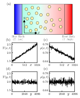
Figure 1: (a) Schematic illustration of the system. The $x$ axis is taken along the direction of the temperature gradient. (b)-(e) Typical one-dimensional temperature and density profiles in the nonequilibrium steady state, observed in the MD simulation. The setup is the same as that of the red curve in Fig. 2 (b), which will be explained later.

Basic properties of long-range correlations.— Before proceeding to the main part of this Letter, we briefly review the LRCs appearing in fluids under temperature gradients. Let us consider a fluid with a uniform temperature gradient along the $x$ axis, as illustrated in Fig. 1 (a). To aid in understanding the phenomenon of LRCs, we first present one-dimensional temperature and density profiles in Figs 1 (b)-(e). These profiles, observed in the MD simulation (described later), illustrate fluctuations of temperature and density around their steady-state profiles at a given time $t$. Here, one-dimensional profiles are obtained from the two-dimensional temperature and density fields, $T(\bm{r},t)$ and $\rho(\bm{r},t)$, by integrating along the $x$ or $y$ direction, for example, $T(x,t):=\int dyT(\bm{r},t)/L_{y}$ or $T(y,t):=\int dxT(\bm{r},t)/L_{x}$. The temperature difference at the boundaries induces a nearly uniform temperature gradient in $T(x,t)$, which in turn leads to a density gradient in $\rho(x,t)$. Moreover, we can clearly observe fluctuations around these steady-state profiles.

The dynamics of such fluctuations at the mesoscopic scale is considered to be effectively captured by fluctuating hydrodynamics, a phenomenological framework that incorporates thermal fluctuations into the hydrodynamic equations [60, 49, 50, 51]. In particular, it has been used to predict fluctuation behavior under temperature gradients [4]. Here, based on this framework, we explain the basic nature of the LRCs in the presence of a temperature gradient. A detailed review of fluctuating hydrodynamics, including the key results used in this Letter, is summarized in Ref. [4].

The main focus of this Letter is density fluctuations. We then calculate the density-density correlation function $\langle\rho(\bm{r},t)\rho(\bm{r}^{\prime},t)\rangle^{\rm th}_{\rm ss}$ or equivalently, the static structure factor $S^{\rm th}(\bm{q})$, defined by

$$\langle\rho(\bm{q},t)\rho(\bm{q}^{\prime},t)\rangle^{\rm th}_{\rm ss}=\rho_{0}S^{\rm th}(\bm{q})(2\pi)^{2}\delta(\bm{q}+\bm{q}^{\prime}),$$ (1)

where $\rho(\bm{r},t)$ is the density field, $\rho(\bm{q},t)$ its Fourier transform, and $\rho_{0}$ the averaged density. Here, we use the superscript ”th” to denote quantities obtained from theoretical discussions.

In equilibrium, $\langle\rho(\bm{r},t)\rho(\bm{r}^{\prime},t)\rangle^{\rm th}_{\rm ss}$ decays exponentially with a correlation length on the microscopic scale. On the hydrodynamic scale, this decay is described by a delta function:

$$\langle\rho(\bm{r},t)\rho(\bm{r}^{\prime},t)\rangle^{\rm th}_{\rm ss}=\rho_{0}S^{\rm th}_{\rm eq}\delta(\bm{r}-\bm{r}^{\prime})\ \ \ {\rm with}\ \ S^{\rm th}_{\rm eq}:=\frac{k_{B}\alpha_{p}^{2}T}{c_{p}-c_{v}}.$$ (2)

Here, $T$ is the temperature, $c_{p}$ the specific heat capacity at constant pressure, $c_{v}$ the specific heat capacity at constant volume, and $\alpha_{p}$ the thermal expansion coefficient. The corresponding static structure factor $S^{\rm th}(\bm{q})$ is then given by:

$$S^{\rm th}(\bm{q})=S^{\rm th}_{\rm eq}.$$ (3)

Fluctuating hydrodynamics predicts that $S^{\rm th}(\bm{q})$ is enhanced due to the temperature gradient $(\nabla T)_{0}$, which is expressed to leading order as follows:

$$S^{\rm th}(\bm{q})=S^{\rm th}_{\mathrm{eq}}+(\nabla T)_{0}^{2}S^{\rm th}_{\mathrm{neq}}(\bm{q}),$$ (4)

where the nonequilibrium correction is proportional to $(\nabla T)_{0}^{2}$. For an infinitely large system, where boundary effects can be neglected, the explicit expression for $S^{\rm th}_{\mathrm{neq}}(\bm{q})$ is given by:

$$S^{\rm th}_{\mathrm{neq}}(\bm{q}) =A_{\mathrm{neq}}\frac{\hat{q}_{y}^{2}}{\bm{q}^{4}}\quad\textrm{with}\quad A_{\mathrm{neq}}=\frac{\alpha_{p}^{2}k_{B}T_{\mathrm{mid}}}{a_{T}(\nu+a_{T})},$$ (5)

where $T_{\mathrm{mid}}$ is the temperature at the center of the system, $\hat{q}_{y}:=q_{y}/|\bm{q}|$, $\nu$ the kinetic viscosity, and $a_{T}$ the thermal diffusivity. This $\bm{q}^{-4}$ divergence in $S^{\rm th}_{\rm neq}(\bm{q})$ is a direct manifestation of the LRCs. Interestingly, it is much stronger than the $\bm{q}^{-2}$ divergence of critical density fluctuations at a liquid-vapor critical point.

The corresponding real-space correlation function is:

$$\frac{\langle\rho(t,\bm{r})\rho(t,\bm{r}^{\prime})\rangle^{\rm th}_{\rm ss}}{\rho_{0}}=S^{\rm th}_{\rm eq}\delta(\bm{r}-\bm{r}^{\prime})+(\nabla T)_{0}^{2}C^{\rm th}_{\mathrm{neq}}(\bm{r},\bm{r}^{\prime}).$$ (6)

The nonequilibrium contribution $C^{\rm th}_{\mathrm{neq}}(\bm{r},\bm{r}^{\prime})$ has a complicated form; for example, for $x=x^{\prime}$ and $y,y^{\prime}\ll L_{y}$, it is:

$$C^{\rm th}_{\mathrm{neq}}(\bm{r},\bm{r}^{\prime})$$

$$=\frac{A_{\mathrm{neq}}L_{y}^{2}}{32\pi^{3}}\left[1+3\Big{|}\frac{y-y^{\prime}}{L_{y}/\pi}\Big{|}^{2}\log\Big{|}\frac{y-y^{\prime}}{L_{y}/\pi}\Big{|}-B\Big{|}\frac{y-y^{\prime}}{L_{y}/\pi}\Big{|}^{2}+\cdots\right]$$ (7)

with $B:=(11-12\gamma)/4$ ($\gamma$: Euler’s constant). Notably, this real-space correlation function lacks a characteristic decay length and its magnitude is proportional to $L_{y}^{2}$. This manifests that the temperature gradient significantly enhances density fluctuations, resulting in the LRCs that persist across the entire system.

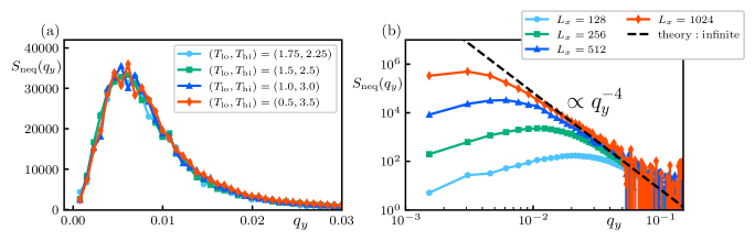
Figure 2: The MD results of the nonequilibrium correction of the static structure factor $S_{\rm neq}(q_{y}):=(S(q_{y})-S_{\mathrm{eq}})/(\nabla T)_{0}^{2}$. (a) Dependence of $S_{\rm neq}(q_{y})$ on the temperature gradients $(\nabla T)_{0}$. We fix the system size at $(L_{x},L_{y})=(512,8192)$ and vary the temperatures at the two ends as $(T_{\mathrm{left}},T_{\mathrm{right}})=(1.75,2.25)$, $(1.5,2.5)$, $(1.0,3.0)$, $(0.5,3.5)$, where the midpoint temperature is fixed at $T_{\mathrm{mid}}:=(T_{\mathrm{left}}+T_{\mathrm{right}})/2=2.0$. The MD results are not influenced by the value of $(\nabla T)_{0}$. (b) Dependence of $S_{\rm neq}(q_{y})$ on the system size $L_{x}$. Data is presented on a log-log scale. We maintain the temperatures at the two ends at $(T_{\mathrm{left}},T_{\mathrm{right}})=(1.5,2.5)$ and vary the system size as $(L_{x},L_{y})=(128,8192)$, $(256,8192)$, $(512,8192)$, $(1024,8192)$. The blue curve presents the same data as the green curve in panel (a), but plotted on a log-log scale. The black dashed line represents the theoretical prediction [Eq. (5)] for an infinitely large system. The MD results approach the theoretical prediction as the wall distance $L_{x}$ increases.

Setting of MD simulations.— We consider a system of $N$ particles confined within a rectangular box of dimensions $[-0.5L_{x},0.5L_{x}]\times[-0.5L_{y},0.5L_{y}]$ (see Fig. 1 (a)). These particles interact via the Weeks–Chandler–Andersen (WCA) potential, given by

$$V_{\mathrm{WCA}}(r)=\begin{cases}4\epsilon\Big{[}\left(\frac{\sigma}{r}\right)^{12}-\left(\frac{\sigma}{r}\right)^{6}+\frac{1}{4}\Big{]},&r\leq 2^{1/6}\sigma\\ 0,&{\mathrm{otherwise}},\end{cases}$$ (8)

where $\epsilon$ and $\sigma$ represent the well depth and atomic diameter, respectively. All particles have the same mass $m$. The particles are confined by walls at $x=-0.5L_{x}$ and $x=0.5L_{x}$, while the periodic boundary condition is applied along the $y$ axis. To establish a temperature gradient along the $x$ axis, we apply Langevin thermostats in the regions $[-0.5L_{x},-0.48L_{x}]$ and $[0.48L_{x},0.5L_{x}]$. The temperatures of these thermostats are, respectively, set to $T_{\mathrm{left}}$ and $T_{\mathrm{right}}$ ($T_{\mathrm{left}}<T_{\mathrm{right}}$), as illustrated in Fig. 1 (a). Our analysis focuses on the bulk region, $\mathcal{B}:=[-0.48L_{x},0.48L_{x}]\times[-0.5L_{y},0.5L_{y}]$, which excludes the thermostatted zones.

We measure physical quantities in units of energy $\epsilon$, length $\sigma$, and time $\tau=\sigma\sqrt{m/\epsilon}$. All the MD simulations are performed by LAMMPS [61]. We fix the density to $\rho=0.7$ and the temperature at the center of the system to $T_{\mathrm{mid}}:=(T_{\mathrm{left}}+T_{\mathrm{right}})/2=2.0$. See SM  for observation protocols and the thermodynamic and transport properties of the fluid.

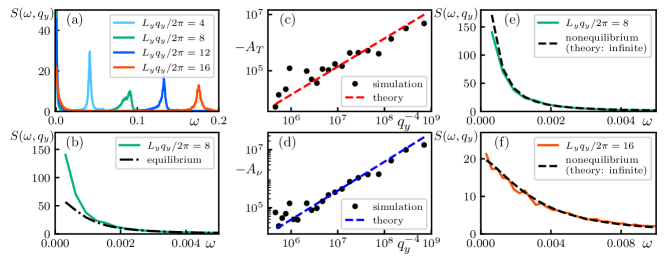
Figure 3: The MD results of the dynamic structure factor $S(\omega,q_{y})$. The parameters are chosen as $(L_{x},L_{y})=(1024,4096)$ and $(T_{\mathrm{left}},T_{\mathrm{right}})=(1.5,2.5)$, corresponding to the red line in Fig. 1 (b). (a) Rayleigh and Brillouin peaks of $S(\omega,q_{y})$ for several wavenumbers, $q_{y}$. (b) $S(\omega,q_{y})$ near the Rayleigh peak for $q_{y}/2\pi=8/L_{y}$. The colored solid curve represents an enlarged view of the data in panel (a), while the black dot-dashed curve represents the corresponding equilibrium result. Nonequilibrium effects dominate the behavior at small $\omega$. (c, d) The $q_{y}^{-4}$ dependence of $A_{T}(q_{y})$ and $A_{\nu}(q_{y})$. The colored dashed lines represent the theoretical predictions [Eq. (15)] for an infinitely large system. The MD results agree accurately with the theoretical predictions, revealing that $A_{T}(q_{y})$ and $A_{\nu}(q_{y})$ exhibit the $q_{y}^{-4}$ divergence. (e, f) Comparison of the Rayleigh peak of $S(\omega,q_{y})$ with theoretical predictions for $q_{y}/2\pi=8/L_{y}$ and $q_{y}/2\pi=16/L_{y}$. The colored solid lines represent the MD results (in particular, the data in panel (e) are replotted from panel (b)). The black dashed curves represent the theoretical predictions under the temperature gradient for an infinitely large system. We observe excellent agreement between the MD results and theoretical predictions.

Direct observation of long-range correlations.— The LRCs can be directly observed through the static structure factor $S(\bm{q})$. In our setup, it is defined as:

$$\langle\rho(t,\bm{q})\rho(t,\bm{q}^{\prime})\rangle_{\rm ss}=\rho_{0}S(\bm{q})(2\pi)^{2}\delta(\bm{q}+\bm{q}^{\prime}),$$ (9)

where $\rho(t,\bm{q}):=\int_{\mathcal{B}}d^{2}\bm{r}\rho(t,\bm{r})e^{-i\bm{q}\cdot\bm{r}}$, $\rho_{0}$ is the average density in the bulk region $\mathcal{B}$, and $\bm{q}=(2\pi n/(0.96L_{x}),2\pi m/L_{y})$ for $n,m\in\mathbb{Z}$. In this study, we focus on the case of $q_{x}=0$, specifically, $S(q_{y}):=S(q_{x}=0,q_{y})$, which is readily accessible through small-angle scattering experiments.

To analyze the nonequilibrium correction to the static structure factor, we decompose $S(q_{y})$ into an equilibrium contribution and a nonequilibrium correction, as suggested by Eq. (4):

$$S(q_{y})=S_{\rm eq}+(\nabla T)_{0}^{2}S_{\rm neq}(q_{y}).$$ (10)

Figure 2 presents the MD results for $S_{\rm neq}(q_{y})$. The typical instantaneous temperature and density profiles are shown in Fig. 1 (b)-(e).

We first investigate the dependence of $S_{\rm neq}(q_{y})$ on the applied temperature gradient $(\nabla T)_{0}$. The results of this analysis are shown in Fig. 2 (a). We observe that $S_{\rm neq}(q_{y})$ collapses onto a single universal curve over a wide range of temperature gradients, indicating that $S_{\rm neq}(q_{y})$ is independent of $(\nabla T)_{0}$. This finding is noteworthy because the temperature dependence of the fluid properties, such as the thermal conductivity, could potentially influence $S_{\rm neq}(q_{y})$, as predicted by fluctuating hydrodynamics in Eq. (5). Indeed, using argon parameters for the WCA potential, our system [red curve in Fig. 2 (a)] experiences a temperature gradient as large as $360\textrm{K}$ over $167\textrm{nm}$. Even under such extreme conditions, $S_{\rm neq}(q_{y})$ is entirely independent of $(\nabla T)_{0}$.

We now turn our attention to the $q_{y}$ dependence of $S_{\rm neq}(q_{y})$. Figure 2 (b) shows the behavior of $S_{\rm neq}(q_{y})$ as we systematically vary the wall separation $L_{x}$ while keeping the temperatures at the ends, $(T_{\mathrm{left}},T_{\mathrm{right}})$, constant. The blue curve presents the same data as the green curve in Fig. 2 (a), but plotted on a log-log scale. The MD results are compared against the theoretical prediction for $S^{\rm th}_{\rm neq}(q_{y})$ [Eq. (5)]. Note that this prediction is for an infinitely large system. For comparison, no fitting parameters were used; the parameters in Eq. (5) were determined from the separate MD simulation . As $L_{x}$ increases, the MD results converge towards the theoretical prediction, clearly revealing the emergence of the $q_{y}^{-4}$ divergence [Eq. (5)]. This direct observation of the $q_{y}^{-4}$ divergence confirms the successful detection of the LRCs in our MD simulation.

Detection of long-range correlations from dynamical structure factor.— Historically, experimental detections of the LRCs under temperature gradients have relied on observations of the dynamic structure factor $S(\omega,\bm{q})$ [13, 14, 15, 16, 17, 18]. This quantity is defined as:

$$S(\omega,\bm{q})=\int_{-\infty}^{\infty}\frac{dt}{2\pi}S(t,\bm{q})e^{-i\omega t}$$ (11)

with $\langle\rho(t,\bm{q})\rho(0,\bm{q}^{\prime})\rangle_{\rm ss}=\rho_{0}S(t,\bm{q})(2\pi)^{2}\delta(\bm{q}+\bm{q}^{\prime})$. The static structure factor $S(\bm{q})$ corresponds to $S(t,\bm{q})$ at $t=0$.

Figure 3 (a) presents the MD results, showing the overall behaviors of $S(\omega,q_{y})$ for various wavenumbers $q_{y}$. For each $q_{y}$, $S(\omega,q_{y})$ exhibits two types of peaks: Rayleigh and Brillouin peaks. The Rayleigh peak is located near $\omega=0$, while the Brillouin peaks are located near $\omega=\pm c_{s}q_{y}$, where $c_{s}$ is the speed of sound. According to fluctuating hydrodynamics, temperature gradients primarily affect the Rayleigh peak. Based on this prediction, we provide an enlarged view of $S(\omega,\bm{q})$ near the Rayleigh peak in Fig. 3 (b), comparing the MD result under the temperature gradient with that for the equilibrium system. As seen in this figure, $S(\omega,\bm{q})$ is enhanced by the temperature gradient for small $\omega$. To identify the presence of the LRCs from this data, we implement two distinct protocols.

The first protocol is to detect, within $S(\omega,\bm{q})$, the counterpart to the $q_{y}^{-4}$ divergence observed in $S(\bm{q})$. To understand the basis of this approach, we present the explicit expressions of $S(t,\bm{q})$ and $S(\omega,\bm{q})$ calculated from fluctuating hydrodynamics for an infinitely large system [4]:

$$S^{\rm th}(t,q_{y}) =S^{\rm th}_{\mathrm{Ray},\mathrm{eq}}\Big{\{}\left(1+(\nabla T)_{0}^{2}A_{T}(q_{y})\right)e^{-a_{T}q_{y}^{2}|t|}$$

$$\hskip 85.35826pt-(\nabla T)_{0}^{2}A_{\nu}(q_{y})e^{-\nu q_{y}^{2}|t|}\Big{\}}$$ (12)

$$S^{\rm th}(\omega,q_{y}) =S^{\rm th}_{\mathrm{Ray},\mathrm{eq}}\Biggl{\{}\left(1+(\nabla T)_{0}^{2}A_{T}(q_{y})\right)\frac{2a_{T}q_{y}^{2}}{\omega^{2}+a_{T}^{2}q_{y}^{4}}$$

$$\hskip 71.13188pt-(\nabla T)_{0}^{2}A_{\nu}(q_{y})\frac{2\nu q_{y}^{2}}{\omega^{2}+\nu^{2}q_{y}^{4}}\Biggr{\}},$$ (13)

where $S^{\rm th}_{\mathrm{Ray},\mathrm{eq}}$ represents the equilibrium contribution from the Rayleigh line, given by

$$S^{\rm th}_{\mathrm{Ray},\mathrm{eq}}=\frac{c_{p}-c_{v}}{c_{p}}S^{\rm th}_{\mathrm{eq}}.$$ (14)

Here, the nonequilibrium correction is proportional to $(\nabla T)_{0}^{2}$, similar to $S(q_{y})$. The coefficients of the nonequilibrium correction, $A_{\nu}(q_{y})$ and $A_{T}(q_{y})$, exhibits the $q_{y}^{-4}$ divergence, given by

$$A_{\nu}(q_{y})=\frac{a_{T}}{\nu}A_{T}(q_{y})=\frac{k_{B}c_{p}}{T_{\mathrm{mid}}(\nu^{2}-a_{T}^{2})}\frac{1}{q_{y}^{4}}.$$ (15)

Since the static structure factor $S(\bm{q})$ is simply $S(t,\bm{q})$ at $t=0$, the $q_{y}^{-4}$ divergence of $A_{\nu}(q_{y})$ and $A_{T}(q_{y})$ manifests the presence of the LRCs.

To detect this $q_{y}^{-4}$ divergence in our MD simulations, we fit $S(\omega,q_{y})$ to Eq. (13) and extract $A_{\nu}(q_{y})$ and $A_{T}(q_{y})$. The results are shown in Figs. 3 (c) and (d), where the obtained $A_{\nu}(q_{y})$ and $A_{T}(q_{y})$ are plotted as a function of $q_{y}^{-4}$. The colored dashed lines represent the theoretical prediction Eq. (15) with the parameters obtained from the separate MD simulation . These figures show a good agreement between the MD results and the theoretical prediction, confirming that both $A_{\nu}(q_{y})$ and $A_{T}(q_{y})$ exhibit a clear $q_{y}^{-4}$ scaling, revealing the presence of LRCs.

The second protocol aims to demonstrate that the MD results for $S(\omega,\bm{q})$ can be quantitatively described by fluctuating hydrodynamics. To this end, Figs. 3 (e) and (f) compare the MD results with the theoretical prediction [Eq. (13) with Eq. (15)]. We present the results for two values of $q_{y}$ to provide unambiguous evidence. These figures show excellent agreement between the MD results and the theoretical prediction. We stress that no fitting parameters were used in these figures; the parameters in Eqs. (13) and (15) were determined from the separate MD simulation . As shown in Fig. 3 (b), $S(\omega,\bm{q})$ clearly contains the nonequilibrium contribution. The excellent agreement shown in Figs. 3 (e) and (f) indicates that fluctuating hydrodynamics accurately describes these nonequilibrium effects. By recalling that fluctuating hydrodynamics predicts the LRCs under temperature gradients [Eq. (5)], we can interpret this excellent agreement as indirect evidence for the presence of the LRCs.

Figure 4: The finite-size effects on the static structure factor $S(q_{y})$, shown as a log-log plot. The inset shows the same data on a linear scale. The parameters are chosen as $(L_{x},L_{y})=(512,8192)$ and $(T_{\mathrm{left}},T_{\mathrm{right}})=(1.5,2.5)$. The black curve represents the MD result, which is the same as that in Fig. 2 (a) The blue dashed and red dot-dashed curves represent the theoretical predictions with the free [20] and rigid boundary conditions [21], respectively. Fluctuating hydrodynamics, irrespective of the boundary conditions, accurately reproduces the shape of the $S_{\rm neq}(q_{y})$ curve obtained from MD simulations.

Approach	Description	Figure	Experimental counterpart
1	Direct observation of $q_{y}^{-4}$ divergence in $S(q_{y})$	Fig. 2 (b)	[19, 23]
2	Observation of $q_{y}^{-4}$ divergence in $S(\omega,q_{y})$	Figs. 3 (c) and (d)	[13, 14, 15, 16, 17, 18]
3	Comparison of $S(\omega,q_{y})$ with fluctuating hydrodynamics	Figs. 3 (e) and (f)	[22, 23]

Table 1: Summary of the three approaches used to investigate the LRCs. Each approach has a corresponding experimental counterpart. A review of early experimental studies can be found in Refs. [3, 4]. More recent experimental investigations are reviewed in Refs. [8, 9, 10].

Discussions.— We address the finite-size effects observed in Fig. 2 (b). These finite-size effects hinder the observation of the LRCs, necessitating large-scale MD simulations. Indeed, as seen in Fig. 2 (b), a large-scale simulation with a wall distance $L_{x}$ of at least $512$ or $1024$ was required to clearly identify the $q_{y}^{-4}$ scaling of $S(q_{y})$. Similar finite-size effects have been previously reported in theoretical [20, 21, 45] and experimental studies [39, 40, 23, 41, 42].

To investigate the origin of these effects, we focus on the MD result for the system with $(L_{x},L_{y})=(512,8192)$ and $(T_{\mathrm{left}},T_{\mathrm{right}})=(1.5,2.5)$ shown in Fig. 2 (a). Figure 4 replots the result of this simulation on a log-log scale (black curve). We compare this MD result with the predictions from fluctuating hydrodynamics, explicitly incorporating the finite-size effects through the application of boundary conditions. We consider two types of boundary conditions: a free boundary condition [20] and a rigid boundary condition [21]. Ortiz de Z‘arate et al. analyzed fluctuating hydrodynamics incorporating these boundary conditions and provided theoretical expressions for $S(\bm{q})$ in Refs. [20, 21]. We will rely on their results to develop our discussion.

Figure 4 reveals two principal mechanisms responsible for the observed finite-size effects. First, the elongated geometry of our system ($L_{x}\ll L_{y}$) restricts the development of the LRCs. This is evident from the remarkable agreement between the shape of the $S_{\rm neq}(q_{y})$ curve obtained from MD simulations and those predicted by fluctuating hydrodynamics, irrespective of the boundary conditions. The theoretical prediction indicates that the maximum intensity occurs at approximately $q_{y}\simeq 1/L_{x}$ [20, 21]. Therefore, this correspondence of the peak positions suggests that a sufficiently large wall distance $L_{x}$ is necessary to induce observable LRCs. Second, the specific boundary conditions applied to the velocity field further suppress the emergence of the LRCs. We find that the MD result is roughly $30\%$ lower than the prediction for the free boundary condition. This discrepancy highlights the suppression of the LRCs by the boundary conditions and suggests that designing boundary conditions could be a strategy for observing stronger LRCs.

Concluding remarks.— In this study, we performed MD simulations to investigate the presence of the LRCs in fluids under temperature gradients. Our simulations employed the three distinct approaches, each with a corresponding experimental counterpart, as summarized in Table 1. First, we directly observed the characteristic $q_{y}^{-4}$ divergence in the static structure factor, $S(q_{y})$, consistent with the experimental observations by Vailati et al. [19] and Takacs et al. [23]. This approach provides direct confirmation of the existence of the LRCs. Second, we examined the dynamic structure factor $S(\omega,q_{y})$ and detected the same $q_{y}^{-4}$ divergence as in $S(q_{y})$. The corresponding experimental observation has been extensively performed since the 1980s [13, 14, 15, 16, 17, 18]. Finally, we compared our MD results for $S(\omega,q_{y})$ with the predictions from fluctuating hydrodynamics and found excellent quantitative agreement. This agreement further validates the existence of the LRCs, whose approach was used experimentally by Takacs et al. [22, 23]. In addition, we observed the similar finite-size effects as those observed in previous experiments [39, 40, 23, 41, 42] From these observations, we conclude that MD simulations are a powerful complementary tool to experiments for investigating LRCs in realistic non-equilibrium situations.

We disregard the role of gravity in fluids under temperature gradients. When fluids are heated from above and cooled from below, gravity suppresses the LRCs, although they persist. Indeed, Vailati et al. [19] and Takacs et al. [23] unambiguously demonstrated the presence of the LRCs even under gravity. Investigating the effect of gravity in MD simulations is left for future work.

S1 MD results for a dilute gas

We present the MD results for a dilute gas. The simulation setup is the same as in the main text, but the density is chosen to be $\rho=0.05$. The fundamental properties of the fluid at this density are summarized in Sec. S3.

S1.1 Static structure factor

Figure S1 illustrates how the nonequilibrium correction of the static structure factor $S_{\rm neq}(q_{y}):=(S(q_{y})-S_{\rm eq})/(\nabla T)_{0}^{2}$ behaves under different temperature gradients and system sizes. In Fig. S1 (a), we keep the system size constant and vary the temperature gradient $(\nabla T)_{0}$. As seen in this panel, $S_{\rm neq}(q_{y})$ exhibits a slight dependence on the temperature gradient. While this dependence is stronger than that observed in the dense liquid [Fig. 2(a)], it is less pronounced than expected, considering that the applied temperature gradients are quite large. In Fig. S1 (b), we maintain the temperatures at the two ends constant and vary the wall distance $L_{x}$. With increasing $L_{x}$, the simulation results converge towards the theoretical prediction for an infinitely large system [Eq. (5)], which is consistent with the case of the dense liquid [Fig. 2(b)]. This convergence confirms that our MD simulations accurately capture the expected $q_{y}^{-4}$ divergence, providing direct evidence of the LRCs even in the dilute gas.

S1.2 Dynamics structure factor

Figure S2 presents a detailed analysis of the dynamical structure factor $S(q_{y},\omega)$. Figure S2 (a) presents the overall behavior of $S(q_{y},\omega)$ for $\omega>0$. Compared to the dense liquid, the dilute gas has a larger sound speed, resulting in a smaller separation between the Rayleigh peak ($\omega=0$) and the Brillouin peaks ($\omega=\pm c_{s}q_{y}$). Figure S2 (b) shows an enlarged view of the Rayleigh peak, comparing the nonequilibrium MD result with the corresponding equilibrium result. We clearly observe the enhancement of the Rayleigh peak due to the temperature gradient.

To quantify this enhancement, we extract $A_{T}(q_{y})$ and $A_{\nu}(q_{y})$ by fitting the MD results for the Rayleigh peak with the theoretical prediction for an infinitely large system [Eq. (13)]. Figures S2 (c) and (d) show $A_{T}(q_{y})$ and $A_{\nu}(q_{y})$ as a function of $q_{y}^{-4}$. In the small $q_{y}$ regime (large $q_{y}^{-4}$), we observe the good agreement between the MD results and the theoretical prediction [Eq. (15)], confirming the expected $q_{y}^{-4}$ divergence of $A_{T}(q_{y})$ and $A_{\nu}(q_{y})$. This is the signature of the LRCs.

However, compared to the dense liquid case, the data in Figure S2 (c) and (d) exhibit more significant deviations from the theoretical prediction. This discrepancy can be attributed to two main factors. First, in the small $q_{y}$ regime, the Rayleigh and Brillouin peaks are not well-separated, making it challenging to isolate the contribution of the Rayleigh peak. Second, in the large $q_{y}$ regime, the enhancement of fluctuations due to the temperature gradient is relatively weak, leading to larger measurement errors. More refined simulations are required to obtain clearer data.

Finally, Figs. S2 (e) and (f) present a direct comparison between the MD results for $S(q_{y},\omega)$ and the theoretical prediction [Eq. (13)] without any fitting parameters. The excellent agreement shown in these panels confirms the validity of fluctuating hydrodynamics for describing nonequilibrium fluctuations even in dilute gas systems.

S1.3 Finite-size effects

Figure S3 presents the finite-size effects on the static structure factor $S(q_{y})$, comparing the MD result with theoretical predictions for free and rigid boundary conditions. The MD result more closely resembles the prediction for the rigid boundary condition. This resemblance is stronger than in the dense liquid discussed in the main text. However, a precise quantitative comparison is difficult due to the limitations of the first-order Galerkin approximation used for the rigid boundary condition. We can at least conclude that our MD setup does not correspond to a system with free boundaries since the theoretical result for the free boundary condition is exact.

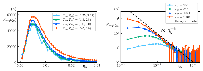
Figure S1: The MD results of the static structure factor $S(q_{y})$, corresponding to Fig. 2 in the main text. (a) Dependence of $S(q_{y})$ on the temperature gradient $(\nabla T)_{0}$. We fix the system size at $(L_{x},L_{y})=(512,8192)$ and vary the temperatures at the two ends as $(T_{\mathrm{lo}},T_{\mathrm{hi}})=(1.75,2.25)$, $(1.5,2.5)$, $(1.0,3.0)$, $(0.5,3.5)$, where the midpoint temperature is fixed at $T_{\mathrm{mid}}:=(T_{\mathrm{lo}}+T_{\mathrm{hi}})/2=2.0$. (b) Dependence of $S(q_{y})$ on the system size $L_{x}$. We maintain the temperatures at the two ends at $(T_{\mathrm{lo}},T_{\mathrm{hi}})=(1.5,2.5)$ and vary the system size as $(L_{x},L_{y})=(256,4096)$, $(512,4096)$, $(1024,4096)$, $(2048,4096)$. The black dashed line represents the theoretical prediction [Eq. (5)] for an infinitely large system.

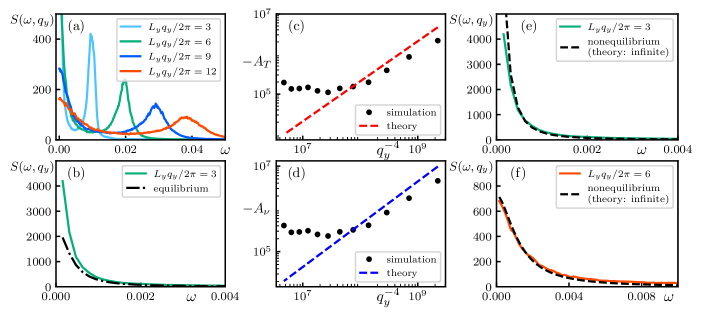
Figure S2: The MD results of the dynamic structure factor $S(\omega,q_{y})$, corresponding to Fig. 3 in the main text. The parameters are chosen as $(L_{x},L_{y})=(2048,4096)$ and $(T_{\mathrm{lo}},T_{\mathrm{hi}})=(1.5,2.5)$, corresponding to the red line in Fig. S2 (a) Rayleigh and Brillouin peaks of $S(\omega,q_{y})$ for several wavenumbers, $q_{y}$. (b) $S(\omega,q_{y})$ near the Rayleigh peak for $q_{y}/2\pi=8/L_{y}$. The colored solid curve represents an enlarged view of the data in panel (a), while the black dot-dashed curve represents the corresponding equilibrium result. (c, d) The $q_{y}^{-4}$ dependence of $A_{T}(q_{y})$ and $A_{\nu}(q_{y})$. The colored solid lines represent the theoretical predictions [Eq. (15)] for an infinitely large system. (e, f) Comparison of the Rayleigh peak of $S(\omega,q_{y})$ with theoretical predictions for $q_{y}/2\pi=6/L_{y}$ and $q_{y}/2\pi=12/L_{y}$. The colored solid lines represent the MD results; in particular, the data in panel (e) are the same as those in panel (b). The black dashed curves represent the theoretical predictions [Eq. (13)] for an infinitely large system.

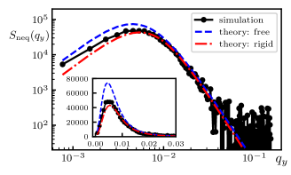
Figure S3: The finite-size effects on the static structure factor $S(q_{y})$, corresponding to Fig. 4 in the main text. This figure is shown as a log-log plot, while the inset shows the same data on a linear scale. The parameters are chosen as $(L_{x},L_{y})=(512,8192)$ and $(T_{\mathrm{lo}},T_{\mathrm{hi}})=(1.5,2.5)$, corresponding to the green line in Fig. 2(a). The black curve represents the MD result, which is the same as those in Fig. 1(a). The blue dashed and red dot-dashed curves represent the theoretical predictions with the free and rigid boundary conditions, respectively.

Density $\rho$	System Size $(L_{x},L_{y})$	Temperatures $(T_{\rm lo},T_{\rm hi})$	Relaxation Loop (steps)	Observation Loop (steps)	Number of Samples
$0.05$	$(256,4096)$	$(1.5,2.5)$	$2,000,000$	$10,000,000$	1152
$0.05$	$(512,4096)$	$(1.5,2.5)$	$5,000,000$	$30,000,000$	1152
$0.05$	$(1024,4096)$	$(1.5,2.5)$	$15,000,000$	$30,000,000$	1440
$0.05$	$(2048,4096)$	$(1.5,2.5)$	$20,000,000$	$40,000,000$	2304
$0.05$	$(512,8192)$	$(1.75,2.25)$	$5,000,000$	$40,000,000$	288
$0.05$	$(512,8192)$	$(1.5,2.5)$	$5,000,000$	$30,000,000$	288
$0.05$	$(512,8192)$	$(1.0,3.0)$	$5,000,000$	$30,000,000$	288
$0.05$	$(512,8192)$	$(0.5,3.5)$	$5,000,000$	$30,000,000$	288
$0.7$	$(128,4096)$	$(1.5,2.5)$	$4,000,000$	$10,000,000$	576
$0.7$	$(256,4096)$	$(1.5,2.5)$	$5,000,000$	$10,000,000$	576
$0.7$	$(512,4096)$	$(1.5,2.5)$	$10,000,000$	$10,000,000$	288
$0.7$	$(1024,4096)$	$(1.5,2.5)$	$15,000,000$	$20,000,000$	288
$0.7$	$(512,8192)$	$(1.75,2.25)$	$10,000,000$	$10,000,000$	144
$0.7$	$(512,8192)$	$(1.5,2.5)$	$10,000,000$	$10,000,000$	72
$0.7$	$(512,8192)$	$(1.0,3.0)$	$10,000,000$	$10,000,000$	72
$0.7$	$(512,8192)$	$(0.5,3.5)$	$10,000,000$	$10,000,000$	72

Table S1: Relaxation steps, observation steps, and the number of samples used to observe the static structure factor $S(q_{y})$ for each set of parameters.

S2 Observation protocol

We provide supplementary information regarding the MD simulations. All simulations were carried out using LAMMPS. We utilized the velocity Verlet algorithm with a time step of $dt=0.002$ for time integration. The particles are confined by walls at $x=-0.5L_{x}$ and $x=0.5L_{x}$, while the periodic boundary condition is applied along the $y$ axis [Fig. 1(a)]. To establish a temperature gradient along the $x$ axis, we applied Langevin thermostats in the regions $[-0.5L_{x},-0.48L_{x}]$ and $[0.48L_{x},0.5L_{x}]$. The dynamics of particles were implemented using different LAMMPS commands depending on their location. In the non-thermostatted region, we used the ”fix nve” command, which solves Newton’s equation of motion. In the thermostatted zones, we used the ”fix langevin” command and simulated Langevin dynamics. To confine the particles within the simulation domain, we introduced walls at $x=-0.5L_{x}$ and $x=0.5L_{x}$. These walls were implemented using the ”fix wall/lj126” command, which models the interaction between the particles and the walls using a Lennard-Jones 12-6 potential.

Two different systems were investigated: a dense liquid with $\rho=0.7$ and a dilute gas with $\rho=0.05$. In both cases, the temperature at the center of the system was maintained at $T_{\mathrm{mid}}:=(T_{\textrm{lo}}+T_{\textrm{hi}})/2=2.0$.

Our simulation procedure consisted of a relaxation phase and an observation phase. As an initial condition, we generated a random spatial configuration of particles and assigned velocities drawn from a Maxwell–Boltzmann distribution at temperature $T$. For larger systems [$(L_{x},L_{y})=(1024,4096)$ for $\rho=0.7$], as an exception, we first performed a pre-equilibration run, where we relaxed the system to thermal equilibrium by applying the Langevin thermostat with temperature $T$ to all particles. To relax the system to a nonequilibrium steady state, we performed a relaxation run with sufficiently large steps. After that, we performed a production run, during which measurements were collected every $250$ steps (equivalently, $250dt=0.5$ time units). Moreover, to enhance the statistical accuracy, multiple independent simulations were performed for each set of parameters, each with different initial conditions and random noise realizations The final results were obtained by averaging over these independent simulations. Table S1 provides the relaxation steps, the observation steps, and the number of samples used to observe the static structure factor $S(q_{y})$ for each set of parameters.

Density $\rho$	Temperature $T$	Pressure $P$	Specific heat capacity at constant volume $c_{v}$	Specific heat capacity at constant pressure $c_{p}$	Thermal expansion coefficient $\alpha_{p}$
0.05	2.0	0.108	1.01	2.00	0.475
0.7	2.0	6.51	1.30	2.22	0.126

Density $\rho$	Temperature $T$	Shear viscosity $\eta$	Kinetic viscosity $\eta/\rho$	Thermal conductivity $\kappa$	Thermal diffusivity $\kappa/\rho c_{p}$
0.05	2.0	0.410	8.20	1.71	17.2
0.7	2.0	1.61	2.30	8.96	5.77

Table S2: the thermodynamic and transport properties of the fluids

S3 Fundamental properties of fluids

Table S2 lists the thermodynamic and transport properties of the fluids. We summarize below how these properties were measured.

S3.1 Specific heat capacity at constant volume $c_{v}$

The specific heat capacity at constant volume $c_{v}$ is defined by

$$c_{v}:=\frac{1}{N}\Biggl{(}\frac{\partial E}{\partial T}\Biggr{)}_{V}.$$ (S1)

where $E$ is the energy, and $N$ is the particle number. To determine $c_{v}$ in our atomic systems from Eq. (S1), we prepare the NVT ensemble with the periodic boundary condition for all directions and observe the energy $E$. The derivative is calculated by fitting the energy data as a function of temperature with a linear function.

The energy is measured for the system size of $(L_{x},L_{y})=(512,512)$ over $64$ or $128$ independent samples. Each sample undergoes the preliminary run with the ”fix nve” command in LAMMPS for the $5000000$ step (i.e. $5000000dt=10000$ time) to reach equilibrium. After that, we collect the energy data every $100$ step during the $5000000$ step (i.e. $5000000dt=10000$ time).

S3.2 Specific heat capacity at constant pressure $c_{p}$

The specific heat capacity at constant pressure $c_{p}$ is defined by

$$c_{p}:=\frac{1}{N}\Biggl{(}\frac{\partial H}{\partial T}\Biggr{)}_{P},$$ (S2)

where $H$ is the enthalpy. To determine $c_{p}$ in our atomic systems from Eq. (S2), we prepare the NPT ensemble with the periodic boundary condition and observe the enthalpy $H:=E+PV$, where $E$ is the energy and $PV$ is the pressure-volume product. The derivative is calculated by fitting the enthalpy data as a function of temperature with a linear function.

The enthalpy is measured for the system size of $(L_{x},L_{y})=(512,512)$ over $64$ or $128$ independent samples. Each sample undergoes the preliminary run with the ”fix npt” command in LAMMPS for the $4000000$ step (i.e. $4000000dt=8000$ time) to reach equilibrium. Subsequently, we switch the time evolution to the Hamiltonian dynamics with the ”fix nve” command in LAMMPS. After an additional $1000000$ step (i.e. $1000000dt=2000$ time), we collect the enthalpy data every $100$ step during the $5000000$ step (i.e. $5000000dt=10000$ time).

S3.3 Thermal expansion coefficient

Thermal expansion coefficient $\alpha_{p}$ quantifies how volume changes per unit temperature change, which is mathematically defined by

$$\alpha_{p}:=\frac{1}{V}\Biggl{(}\frac{\partial V}{\partial T}\Biggr{)}_{P}=-\frac{1}{\rho}\Biggl{(}\frac{\partial\rho}{\partial T}\Biggr{)}_{P}$$ (S3)

where $V$ is the area of the system. The determination of $\alpha_{p}$ in our atomic systems is performed simultaneously with the one for specific heat capacity $c_{p}$. We measure the area as the function of the temperature and estimate the thermal expansion coefficient $\alpha_{p}$ from Eq. (S3).

S3.4 Shear viscosity

The shear viscosity $\eta$ is defined through the constitute equation of fluids

$$\Pi_{ij}=p\delta_{ij}+\rho v_{i}v_{j}-\eta\Biggl{(}\frac{\partial v_{j}}{\partial x_{i}}+\frac{\partial v_{i}}{\partial x_{j}}-\delta_{ij}\frac{\partial v_{k}}{\partial x_{k}}\Biggr{)}-\zeta\delta_{ij}\frac{\partial v_{k}}{\partial x_{k}}$$ (S4)

where $\Pi_{ij}$ represents the momentum flux. To determine the shear viscosity $\eta$ in our atomic systems, we use the simpler form of the constitute equation in the Couette flow setup as

$$\Pi_{xy}=\eta\frac{\partial v^{x}}{\partial y}$$ (S5)

The measurement is performed for the system with $(L_{x},L_{y})=(512,512)$. We perform the $128$ independent runs to take an ensemble average. Each of the $128$ samples undergoes the relaxation run for the $500000$ step (i.e. $500000dt=10000$ time). After the system reached the nonequilibrium steady state, we observe the shear stress $\Pi_{xy}(x)$ and the velocity field $v_{x}(x)$ every $1000$ step during the $500000$ step. Then, the shear viscosity is then estimated as a ratio of the shear stress to the velocity gradient.

S3.5 Thermal conductivity

Thermal conductivity $\kappa$ is defined through Fourier’s law

$$\bm{q}=-\kappa\frac{\partial T}{\partial\bm{x}},$$ (S6)

where $\bm{q}$ represents the heat flux. To determine $\kappa$ in our atomic systems, we use the same setup as given in the main text (Fig. 1(a)). Because the heat flows only along the $x$ axis, we can apply the simpler form of Fourier’s law

$$q_{x}=-\kappa\frac{\partial T}{\partial x}.$$ (S7)

The measurement is performed for the system with $(L_{x},L_{y})=(512,512)$. We perform the $128$ independent runs to take an ensemble average. Each of the $128$ samples undergoes the relaxation run for the $10000000$ step (i.e. $10000000dt=10000$ time). After the system reached the nonequilibrium steady state, we observe the heat flux $q_{x}(x)$ and the temperature field $T(x)$ every $1000$ step during the $15000000$ step. Then, the thermal conductivity is then estimated as a ratio of the heat flux to the temperature gradient.