Autonomous Quantum Heat Engine Enabled by Molecular Optomechanics and Hysteresis Switching

Abstract

By integrating molecular optomechanics with molecular switches, we propose a scheme for a molecular quantum heat engine that operates autonomously through hysteretic feedback without external driving or modulation. Through a comparative analysis conducted within both semiclassical and fully quantum frameworks, we reveal the influence of quantum properties embedded within the autonomous control elements on the operational efficiency and performance of this advanced molecular machine.

Introduction.—Artificial Molecular Machines (AMMs), are bottom-up designed nanomachines aimed at mimicking the behavior of molecular proteins in living systems, efficiently converting various forms of energy into mechanical work to drive essential biological processes Jülicher et al. (1997); Schliwa and Woehlke (2003); Kassem et al. (2017); Iino et al. (2020); Vale (2003); Hernandez et al. (2004); Balzani et al. (2006); Hugel et al. (2002); Harris et al. (2018); Torres-Cavanillas et al. (2024); Avellini et al. (2012); Yao et al. (2020); Chen et al. (2016); Merino et al. (2018); Goodwin et al. (2017); Hicks (2011); Shepherd et al. (2013); Nguyen et al. (2007); Kornilovitch et al. (2002); Emberly and Kirczenow (2003); Martin et al. (2006); Thijssen et al. (2006); Litman and Rossi (2020); Wang et al. (2023); Venkataramani et al. (2011). Advances in nanofabrication have markedly improved our ability to detect and manipulate molecules on surfaces, facilitating the transition of AMMs from traditional solution-phase chemistry to surface and interface physics. Electric, magnetic, and optical energy have emerged as viable alternatives to chemical energy for powering AMMs. In particular, the strong coupling between molecules and light achievable in minute plasmonic cavities has led to the emerging field of molecular optomechanics Benz et al. (2016); Esteban et al. (2022); Roelli et al. (2016); Ashrafi et al. (2019); Lombardi et al. (2018); Schmidt et al. (2016), where optomechanical coupling strengths can exceed those of state-of-the-art microfabricated devices by several orders of magnitude and provide a promising platform to realize quantum AMMs operable at room temperature.

Power and control are two essential functional components of AMMs, resulting in considerable research interest in molecular motors Jülicher et al. (1997); Schliwa and Woehlke (2003); Kassem et al. (2017); Iino et al. (2020); Vale (2003); Hernandez et al. (2004); Balzani et al. (2006) and switches Hugel et al. (2002); Harris et al. (2018); Torres-Cavanillas et al. (2024); Avellini et al. (2012); Yao et al. (2020); Chen et al. (2016); Merino et al. (2018); Goodwin et al. (2017); Hicks (2011); Shepherd et al. (2013); Nguyen et al. (2007); Kornilovitch et al. (2002); Emberly and Kirczenow (2003); Martin et al. (2006); Thijssen et al. (2006); Litman and Rossi (2020); Wang et al. (2023); Venkataramani et al. (2011). The former function essentially as heat engines, akin to proteins that extract energy from the environment, convert a fraction into productive motion, and dissipate the rest as heat. The latter are molecules capable of reversibly transitioning between two or more stable states in response to environmental stimuli. In this work we theoretically demonstrate a molecular optomechanical platform that integrates these two components to operate an autonomous optomechanical quantum heat engine, a key building block for the development of more intricate and functional quantum AMMs powered by light.

Much work in traditional optomechanics has been devoted to quantum versions of classical reciprocating engines Blickle and Bechinger (2012); Quan et al. (2007); Feldmann and Kosloff (2003); Zhang et al. (2014); Peterson et al. (2019); Roßnagel et al. (2016); Serra-Garcia et al. (2016). But due to their periodic external control consuming more energy than produced, there is a growing interest in autonomous quantum heat engines, inspiring several proposals featuring quantum versions of clocks and flywheels, analogous to classical automatic control Carollo et al. (2020); Elouard et al. (2015); Serra-Garcia et al. (2016); Seah et al. (2018); Mari et al. (2015); Tonner and Mahler (2005); Roulet et al. (2017); Toyabeme and Izumida (2020).

We focus here on the use of feedback control as an automatic control mechanism as there are already extensive architectures that integrate bistability and hysteresis into molecular machines to create hysteretic molecular switches Torres-Cavanillas et al. (2024); Yao et al. (2020); Chen et al. (2016); Goodwin et al. (2017); Hicks (2011); Shepherd et al. (2013); Kornilovitch et al. (2002). These switches can establish a history-dependent negative feedback control loop for the quantum heat engine. Compared to the more common measurement feedback control Zhang et al. (2017), this method avoids consuming additional energy when storing and amplifying measured signals. And importantly, optomechanical heat engines controlled by such a hysteretic molecular switch also offer a unique opportunity to investigate changes in the nature of automatic control and work extraction as they transition from the classical to the quantum regime, a consequence of their ultrasmall size and remarkable robustness to thermal noise. As we will show, when both quantum tunneling in the molecular switch and the quantum correlations between the engine and feedback controller are taken into account, the autonomous molecular engine exhibits distinct characteristics in terms of output power, operational parameter range, and plasmon statistics.

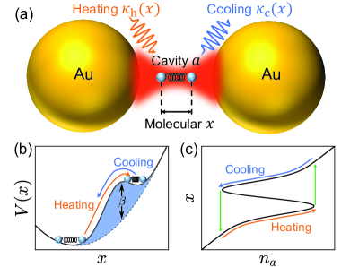
Figure 1: (Color online) (a) Autonomous molecular heat engine with a molecular switch in a plasmonic cavity (gold spheres), coupled via dispersive and dissipative optomechanics. (b) The effective potential of the hysteretic molecular switch, where radiation pressure triggers the transition between states. (c) Heat engine’s working cycle, featuring a hysteresis loop in the molecular reaction coordinate $x$, driven by radiation pressure proportional to plasmon number $n_{\rm a}$. The parameters are $\theta=\hbar\omega_{\rm m}x_{0}^{-1},L=x_{0},\beta=2\hbar\omega_{\rm m}$, where $x_{0}=\sqrt{\hbar/2m\omega_{\rm m}}$ represents the vacuum fluctuation of the reaction coordinate.

Model—Hysteretic molecular switches are unique molecules that transit between stable configurations at different thresholds, depending on the direction of the switch. This results in hysteretic changes in properties such as adsorption/desorption Chen et al. (2017); Merino et al. (2018), conductivity Lotze et al. (2012); Thijssen et al. (2006); Halbritter et al. (2008); Trouwborst et al. (2009); Kornilovitch et al. (2002); Emberly and Kirczenow (2003); Martin et al. (2006); Xia et al. (2024), and magnetism Goodwin et al. (2017); Sano (1997); Torres-Cavanillas et al. (2024); Hicks (2011); Shepherd et al. (2013); Venkataramani et al. (2011) in response to chemical, electrical, or optical stimuli. The switching dynamics can be modeled by an oscillator in a double-well potential

$$V(\hat{x})=\frac{1}{2}m\omega_{\rm m}^{2}\hat{x}^{2}+\theta\hat{x}+\beta e^{-\hat{x}^{2}/L^{2}},$$ (1)

where $\hat{x}$ is the molecular reaction coordinate, an abstract 1D representation of molecular configuration changes in response to stimuli, often related to geometric parameters such as molecular bond length or bond angle, and $m$ and $\omega_{\rm m}$ represent the oscillator’s effective mass and frequency, respectively. The parameter $\theta$ accounts for the potential asymmetry, while $\beta$ and $L$ characterize the energy barrier’s height and width. The two energy minima correspond to bistable molecular configurations that originate directly from distinct internal vibrational states Thijssen et al. (2006); Shepherd et al. (2013), alternative molecular isomeric states Hugel et al. (2002); Avellini et al. (2012); Chen et al. (2016); Goodwin et al. (2017); Hicks (2011); Nguyen et al. (2007); Kornilovitch et al. (2002); Venkataramani et al. (2011), or varying adsorption states on surfaces Merino et al. (2018); Emberly and Kirczenow (2003); Martin et al. (2006); Litman and Rossi (2020); Wang et al. (2023); Xia et al. (2024). As a result of the potential’s asymmetry, the required stimulus energy differs during state switching, as illustrated in Fig. 1(b).

We proceed by embedding the molecular switch within a plasmonic nanocavity crafted from gold nanospheres (Fig. 1(a)) – or alternative structures exhibiting surface-enhanced Raman scattering effects Esteban et al. (2022); Roelli et al. (2016); Ashrafi et al. (2019); Lombardi et al. (2018); Schmidt et al. (2016); Benz et al. (2016) – in such a way that the reaction coordinate aligns with the Raman-excitable molecular vibration. This results in the cavity optomechanical coupling between the local plasmon field ($\hat{E}\sim\hat{a}+\hat{a}^{\dagger}$) and the induced Raman dipole ($\hat{d}\sim\hat{x}\hat{E}$) of the molecule, and variations in the intensity of the plasmon field can then stimulate a switch of the molecule between two states of the bistable potential $V(\hat{x})$. At the same time, this coupling also results in a shift and broadening in the cavity mode frequency, phenomena that are respectively referred to as dispersive and dissipative cavity optomechanical effects Primo et al. (2020); Sankey et al. (2010); Kyriienko et al. (2014); Gu and Li (2013); Li et al. (2009).

When coupling this system to both a hot and a cold reservoir that exhibit distinct, narrowly peaked frequency spectra, we can then exploit the molecular switch as a feedback controller to automate the thermodynamic cycle of the optomechanical heat engine. To see how this works, assume that the cavity plasmon mode is initially at the peak frequency of the hot reservoir. The cavity mode will therefore be energized, and the increase in radiation pressure triggers a molecular state transition via dispersive optomechanical coupling. As a result the cavity mode frequency will be shifted in such a way that it is now at the peak frequency of the cold reservoir, leading to the cooling of the cavity mode. The reduced radiation pressure triggers a reversed molecular transition back to its initial state. At that point the mode frequency has returned at the peak frequency of the hot reservoir, and the next heating-cooling sequence can proceed, establishing a feedback control loop. The hysteresis of the molecular switch in Fig. 1(c), enabling periodic self-sustaining oscillations under suitable conditions, is key to maintaining the loop.

This heat engine can be modeled as a coupled system of three oscillators, the first one describing the molecule and the other two a pair of cavity modes of distinct frequencies, which can be realized through meticulously designed dielectric structures such as hybrid cavity-antenna resonators Shlesinger et al. (2021, 2023); Abutalebi et al. (2024). To simplify the thermodynamic analysis, we combine the two coupled cavity modes into a normal mode $\hat{a}$, reducing the analysis to a two-oscillator model. The full model and detailed derivation are provided in the supplementary material (SM). The dynamics of the system is then governed by the master equation

$$\dot{\rho}=-\frac{i}{\hbar}[\hat{H}_{\rm om},\rho]+(\hat{\mathcal{L}}_{\rm h}+\hat{\mathcal{L}}_{\rm c}+\hat{\mathcal{L}}_{\gamma})\rho,$$ (2)

where the total Hamiltonian is given by

$$\hat{H}_{\rm om}=\hbar(\omega_{\rm a}+g_{\omega}\hat{x})\hat{a}^{\dagger}\hat{a}+\frac{\hat{p}^{2}}{2m}+V(\hat{x}),$$ (3)

where $g_{\omega}$ represents the dispersive optomechanical coupling strength. The Lindblad superoperators $\hat{\mathcal{L}}_{j=\rm h,c}$ describe the dissipation of the normal cavity mode $\hat{a}$ due to the hot and cold reservoirs, respectively. Accounting for the fact that the molecular motion alters the proportion of the two cavity modes in the normal mode $a$ results in an $x$-dependent dissipation rate—a dissipative optomechanical coupling effect— they take the form

$$\hat{\mathcal{L}}_{j}\rho=(\bar{n}_{j}+1)\mathcal{D}\Big{[}\sqrt{\kappa_{j}(\hat{x})}\hat{a}\Big{]}\rho+\bar{n}_{j}\mathcal{D}\Big{[}\sqrt{\kappa_{j}(\hat{x})}\hat{a}^{\dagger}\Big{]}\rho,$$ (4)

$j=\{{\rm h,c}\}$, where the Lindblad dissipator is defined as $\mathcal{D}[\hat{O}]\rho=\hat{O}\rho\hat{O}^{\dagger}-\frac{1}{2}\{\hat{O}^{\dagger}\hat{O},\rho\}$, and $\bar{n}_{\rm h,c}$ are the thermal occupation numbers of the two reservoirs. As discussed in the SM, we approximate their complex expressions following the normal mode transformation by the smooth logistic functions

$$\kappa_{\rm h,c}(\hat{x})=\frac{\kappa_{0}}{1+e^{\pm g_{\kappa}\hat{x}}}.$$ (5)

Here $g_{\kappa}$ and $\kappa_{0}$ denote the dissipative optomechanical coupling strength and maximum dissipation rate achievable by the cavity mode. In addition the environmental impact on the molecular switch is characterized by Brownian noise in the form of a Caldeira-Leggett superoperator,

$$\hat{\mathcal{L}}_{\gamma}[\rho]=-\frac{i\gamma}{2\hbar}\Big{[}\hat{x},\{\hat{p},\rho\}\Big{]}-\frac{\gamma}{\hbar}\left(n_{\mathrm{th}}+\frac{1}{2}\right)\Big{[}\hat{x},[\hat{x},\rho]\Big{]}.$$ (6)

In the present scheme, the cavity mode, coupled to the molecular switch and two reservoirs, serves as the working fluid of the heat engine. According to the first law of thermodynamics Alicki (1979); Kosloff and Levy (2014); Kosloff (2013), the heat engine’s instantaneous power $\mathcal{P}$ is the net heat transfer rate, given by

$$\mathcal{P}=\dot{Q}_{\rm h}+\dot{Q}_{\rm c}={\rm Tr}[\hat{H}_{\rm a}^{\rm eff}\hat{\mathcal{L}}_{\rm h}\rho]+{\rm Tr}[\hat{H}_{\rm a}^{\rm eff}\hat{\mathcal{L}}_{\rm c}\rho],$$ (7)

where $\hat{H}_{\rm a}^{\rm eff}=\hbar(\omega_{\rm a}+g_{\omega}\hat{x})\hat{a}^{\dagger}\hat{a}$ is the Hamiltonian of the cavity mode. The detailed thermodynamics analysis is included in the SM. Note that there is no explicit workload or battery in this system, and all the work output is absorbed by the molecular switch, i.e., the feedback controller.

Classical switch—For large molecules and/or high operating temperatures, the molecular switch behaves as a classical bistable oscillator. In this limit we substitute the operator $\hat{x}$ with its mean value $x$, whose evolution is governed by a classical Langevin equation which can be simplified to the overdamped equation of motion

$$\dot{x}=-\frac{1}{m\gamma}(\partial_{x}V+\hbar g_{\omega}n_{\rm a}).$$ (8)

The evolution of the mean plasmon number, $n_{\rm a}={\rm Tr}[\rho_{\rm a}\hat{a}^{\dagger}\hat{a}]$, is then captured by the equation

$$\dot{n}_{\rm a}=-\kappa_{0}(n_{\rm a}-\bar{n}_{\rm eff}(x)),$$ (9)

where the equilibrium photon number $\bar{n}_{\rm eff}(x)=(\kappa_{\rm h}(x)\bar{n}_{\rm h}+\kappa_{\rm c}(x)\bar{n}_{\rm c})/\kappa_{0}$, depends on the reaction coordinate $x$ of the molecular switch. These coupled differential equations regulate the classical dynamics of the autonomous molecular optomechanical heat engine, with periodic, self-sustaining oscillations arising spontaneously under favorable parametric conditions, see SM for more details.

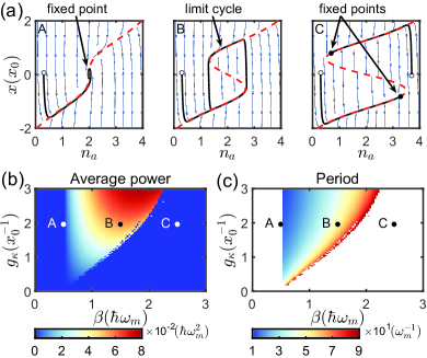
Figure 2: (Color online) (a) Phase trajectories (black lines) in $(n_{\rm a},x)$ phase space for cases A, B, C. The hollow/solid dots mark initial/final states and the blue arrows are streamlines $(\dot{n}_{\rm a},\dot{x})$. The contour plots show the engine power $P$ (b) and working cycle period $T$ (c) as functions of $g_{\kappa}$ and $\beta$. The system parameters are $\kappa_{0}=0.05\omega_{\rm m}$, $\gamma=0.5\omega_{\rm m}$, $n_{\rm c}=0$, $n_{\rm h}=4$, $g_{\omega}=-\omega_{\rm m}x_{0}^{-1}$, and $\omega_{\rm a}=100\omega_{\rm m}$.

For a classical switch, combining Eqs. (7) and (2) simplifies the expression for the power to $\mathcal{P}=-\hbar g_{\omega}n_{\rm a}\dot{x}$, so that the average power output of the heat engine becomes $P=\frac{1}{T}\oint\mathcal{P}dt$, where the integration encompasses a complete working cycle of the heat engine, that is one period $T$ of the self-sustaining oscillations.

Figs. 2(b) and (c) show how the energy barrier height $\beta$ and dissipative coupling strength $g_{\kappa}$ affect $P$ and $T$. Optimal engine performance requires a high $g_{\kappa}$ and moderate $\beta$. Low barrier heights $\beta$ weaken the hysteresis loop, while excessive $\beta$ hinders optomechanical switching. Fig. 2(a) illustrates the system dynamics at points A (low $\beta$), B (moderate $\beta$), and C (high $\beta$) in the 2D phase space $(n_{\rm a},x)$. For B, the equilibrium positions derived from Eq. (8) form a hysteresis loop with two stable branches (red dashed line), as confirmed by the streamlines $(\dot{n}_{\rm a},\dot{x})$ (blue arrows). Any phase trajectory (black line) evolves to a limit cycle, indicating self-oscillations between branches. In contrast, for the parameters of A the system converges to a fixed point (rest state). Finally, for C the system exhibits two fixed points, the final state depending on the specific initial conditions.

A distinct boundary exists between the operational and non-operational domains of the autonomous heat engine. This boundary can be derived through an analysis of the self-sustaining oscillation’s trigger threshold from Eqs. (9) and (8), resulting in two specific curves, $\hbar g_{\omega}\bar{n}_{\rm eff}(x_{\pm})+\partial_{x}V(x_{\pm})=0$, where $x_{\pm}$ represent the two inflection points of potential $V(x)$ (see SM for more details). The output work $W$ approaches its maximum value near this boundary, but the power $P$ decreases due to the simultaneously maximized period $T$.

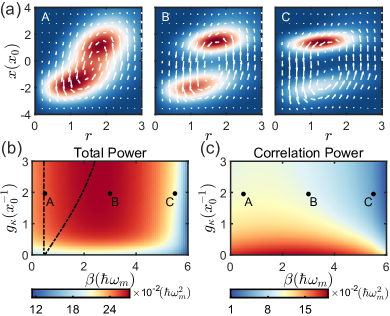
Figure 3: (Color online) (a) Quasi-probability density $\tilde{\mathcal{Q}}(r,x)$ for cases corresponding to points A, B, and C in (b), respectively, with white arrows indicating the quasi-probability flows. The contour plots illustrate (b) the steady-state engine power and (c) the contribution from quantum correlation, within the framework of a quantum switch, where the dashed line outlines the boundary separating the classical operational domain. The parameters utilized are identical to those in Fig. 2, and $n_{\rm th}=0$.

Quantum switch—For small molecules operating at low temperatures the dynamics of the engine are governed by the full master equation (2), which results in its evolution toward a steady state density operator $\rho_{\rm s}$. This means in particular that the mean field intensity of the plasmonic field and molecular reaction coordinate no longer exhibit a bistable behavior Drummond and Walls (1980), so the heat engine can no longer be understood in terms of phase space trajectories as depicted in Fig. 2. Rather, its operation, and more specifically the exchange of heat and work that still persist under these conditions, rely now fully on the quantum properties of the molecule-field system, most importantly on quantum tunneling within the double-well potential, but also the quantum correlations that it develops with the cavity mode.

The steady-state instantaneous power $\mathcal{P}_{\rm s}$, as defined in Eq. (7), is depicted in Fig. 3(b). In contrast to the classical case, no boundary circumscribes the operational region. This is because the molecular switch operates via quantum tunneling, even when the plasmon number $n_{\rm a}$ is insufficient to propel the molecule across the barrier $\beta$. Moreover, the power significantly exceeds that of the classical case due to the incorporation of both the mechanical work’s power and an additional energy flow that is overlooked in the classical approach but fosters quantum correlations between the molecule and the plasmon Francica et al. (2017); Manzano et al. (2018). This is exemplified by the difference $-(\hbar g_{\omega}/m)(\langle\hat{a}^{\dagger}\hat{a}\hat{p}\rangle-\langle\hat{a}^{\dagger}\hat{a}\rangle\langle\hat{p}\rangle)$ illustrated in Fig. 3(c).

Although $\mathcal{P}_{\rm s}$ is independent of time, the quantum dynamics of the engine can be described by quasi-probability distributions and flows in phase space. The former is represented by a modified Husimi $Q$-function

$$\tilde{\mathcal{Q}}(r,x)=\frac{1}{\pi}\int_{0}^{2\pi}\langle{re^{i\phi},x}|\rho_{\rm s}|{re^{i\phi},x}\rangle{r}\,{\rm d}\phi,$$ (10)

where $|re^{i\phi}\rangle$ denotes coherent states of the cavity mode with amplitude $r$ and phase $\phi$, while $|x\rangle$ represents eigenstates of the molecular reaction coordinate operator. The quasi-probability flow is characterized by the vector field $(u(r,x),v(r,x))$, where $u$ and $v$ represent flow amplitudes in the $r$ and $x$ coordinates, respectively, and are derived from (see SM for more details)

$$u(r,x) = -\int_{0}^{r}\tilde{D}(r^{\prime},x){\rm d}r^{\prime},\quad v(r,x)=\int_{-\infty}^{x}\tilde{D}(r,x^{\prime}){\rm d}x^{\prime},$$

$$\tilde{D}(r,x) = \frac{1}{\pi}\int_{0}^{2\pi}\langle{re^{i\phi},x}|(\hat{\mathcal{L}}_{\rm h}\rho_{\rm s}+\hat{\mathcal{L}}_{\rm c}\rho_{\rm s})|{re^{i\phi},x}\rangle{r}\,{\rm d}\phi.$$ (11)

Analogous to the classical case, Fig. 3(a) illustrates the quasi-probability distribution and flow for cases involving low, medium, and high energy barriers ($\beta$). In case A (low $\beta$), the double-well potential collapses into a single well, but non-zero displacement fluctuations sustain the quasi-probability flow, keeping the engine operational. In contrast, case C (high $\beta$) displays pronounced quasi-probability localization, as the barrier impedes probability transfer between wells, effectively stalling the engine. Case B (medium $\beta$) exhibits a bimodal quasi-probability distribution, where the flow lines signify the dynamics of quasi-probability exchange between the peaks, reminiscent of the hysteresis loop in the classical case.

In contrast to the classical scenario, where the cavity mode maintains thermal states throughout the engine’s operational cycle, the quantum nature of the molecular switch results in the emergence of steady-state quantum correlations and in nonclassical statistics for the cavity mode. As illustrated in Fig. 4(b), the second-order correlation function, $g^{(2)}(0)=\langle\hat{a}^{\dagger}\hat{a}^{\dagger}\hat{a}\hat{a}\rangle/\langle\hat{a}^{\dagger}\hat{a}\rangle^{2}$, dips below unity as the optomechanical couplings $g_{\omega}$ and $g_{\kappa}$ intensify, a phenomenon that coincides with the presence of negative Wigner functions in Fig. 4(a). The negativity of the Wigner function underscores the pronounced nonclassical characteristics of the heat engine.

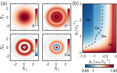
Figure 4: (a) Wigner function of the cavity mode for four selected points indicated in (b). (b) Second-order field correlation $g^{(2)}(0)$ of the cavity mode as a function of optomechanical couplings $g_{\omega}$ and $g_{\kappa}$, with $g^{(2)}(0)=1$ indicated by a dashed line. All parameters as in Fig. 2, except for $\beta=4\hbar\omega_{\rm m}$.

Conclusion.—In summary, we have proposed and analyzed a quantum AMM that combines molecular optomechanical coupling and hysteretic molecular switches to achieve an autonomous quantum heat engine. The inherent nonclassical features of the molecular switch, encompassing quantum fluctuations, correlations, and tunneling, profoundly influence the autonomous operation and overall performance of the heat engine. This work also validates the potential of molecular optomechanical systems to serve as a platform for exploring AMMs that transcend the classical-to-quantum boundary. Future research endeavors will explore the diverse applications of molecular optomechanics in other AMMs such as molecular shuttles and molecular logic gates while also investigating their performance at the quantum scale.

Supplemental Materials

I Model and Master Equation

In a plasmonic nanocavity, well-designed dielectric structures (e.g., hybrid cavity-antenna architecture, see Ref[58,59] in the main text) enable strong coupling between photonic and plasmonic modes, causing spectrum splitting. A molecular switch inside alters mode frequencies, leading to resonance anticrossing and mode property shifts between photonic and plasmonic states. The following total Hamiltonian describes this phenomenon

$$\hat{H}_{\rm OM}=\hbar(\omega_{A}+g_{A}\hat{x})\hat{A}^{\dagger}\hat{A}+\hbar(\omega_{B}+g_{B}\hat{x})\hat{B}^{\dagger}\hat{B}+\frac{\hbar g}{2}(\hat{A}^{\dagger}\hat{B}+\hat{A}\hat{B}^{\dagger})+\hat{H}_{\rm m},$$ (S1)

where $\hat{A}$ and $\hat{B}$ denote the annihilation operators for a pair of coupled plasmonic and photonic modes, respectively, with frequencies $\omega_{A}$ and $\omega_{B}$. The coefficients $g_{A}$, $g_{B}$, and $g$ represent the molecular optomechanical coupling strengths and the photon-plasmon coupling strength, respectively. Additionally, $\hat{H}_{\rm m}=\frac{\hat{p}^{2}}{2m}+\hat{V}(\hat{x})$ represents the Hamiltonian of the molecular switch.

By employing a Bogoliubov transformation, the Hamiltonian pertaining to the cavity modes can be diagonalized into two distinct, non-interacting bosonic normal modes,

$$\hat{H}_{\rm OM}=\hbar\omega_{a}(\hat{x})\hat{a}^{\dagger}\hat{a}+\hbar\omega_{b}(\hat{x})\hat{b}^{\dagger}\hat{b}+\hat{H}_{\rm m},$$ (S2)

where the frequencies of these normal modes, $\omega_{a}$ and $\omega_{b}$, are dependent on the molecular reaction coordinate $\hat{x}$,

$$\omega_{a,b}=\frac{1}{2}\left[\omega_{A}+\omega_{B}+(g_{A}+g_{B})\hat{x}\pm\sqrt{\left(\omega_{A}-\omega_{B}+(g_{A}-g_{B})\hat{x}\right)^{2}+g^{2}}\right].$$ (S3)

The Bogoliubov transformation matrix is expressed as

$$\begin{bmatrix}\hat{a}\\ \hat{b}\end{bmatrix}=\begin{bmatrix}u_{11}&u_{12}\\ u_{21}&u_{22}\end{bmatrix}\begin{bmatrix}\hat{A}\\ \hat{B}\end{bmatrix}=\begin{bmatrix}\frac{-g}{\sqrt{2\Omega^{2}+2\Omega\Delta}}&\frac{\Omega+\Delta}{\sqrt{2\Omega^{2}+2\Omega\Delta}}\\ \frac{g}{\sqrt{2\Omega^{2}-2\Omega\Delta}}&\frac{\Omega-\Delta}{\sqrt{2\Omega^{2}-2\Omega\Delta}}\end{bmatrix}\begin{bmatrix}\hat{A}\\ \hat{B}\end{bmatrix},$$ (S4)

where the matrix elements are also functions of $\hat{x}$ through the relations $\Omega=\sqrt{\Delta^{2}+g^{2}}$ and $\Delta=\omega_{A}-\omega_{B}+(g_{A}-g_{B})\hat{x}$. The inverse transformation is given by

$$\begin{bmatrix}\hat{A}\\ \hat{B}\end{bmatrix}=\begin{bmatrix}u_{11}&u_{21}\\ u_{12}&u_{22}\end{bmatrix}\begin{bmatrix}\hat{a}\\ \hat{b}\end{bmatrix}.$$ (S5)

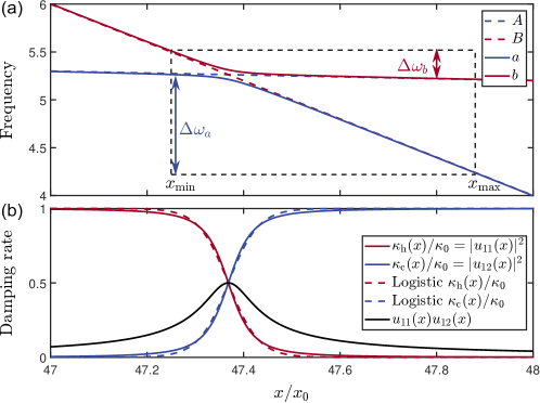
Figure S1: (color online) (a) Frequency comparison of bared modes $A,B$ (dashed lines) and normal modes $a,b$ (solid lines) as functions of the molecular reaction coordinate $x$. (b) Comparison of exact (solid lines) and approximated (dashed lines) dissipation rates. The parameters are defined as $\omega_{A}=10^{2}g$, $\omega_{B}=10^{3}g$, $g_{A}=-gx_{0}^{-1}$, and $g_{B}=-20gx_{0}^{-1}$, where $x_{0}=\sqrt{\hbar/2m\omega_{m}}$ represents the vacuum fluctuation of the reaction coordinate.

As depicted in Fig. S1(a), the frequencies of the normal modes $a$ and $b$ undergo transitions between photon-like and plasmon-like characteristics as $\hat{x}$ varies. Similarly, their environment transitions between one governed by a hot plasmon reservoir and another dominated by a cold photon reservoir. This behavior becomes apparent when applying Bogoliubov transformations to the dissipation dynamics of modes $A$ and $B$.

The derivation proceeds as follows: the dissipation of modes $A$ and $B$ is characterized by the application of superoperators $\hat{\mathcal{L}}_{A,B}$ on the density matrix $\rho$,

$$\hat{\mathcal{L}}_{O}\rho=\kappa_{O}(\bar{n}_{O}+1)\mathcal{D}[\hat{O}]\rho+\kappa_{O}\bar{n}_{O}\mathcal{D}[\hat{O}^{\dagger}]\rho,$$ (S6)

where $\mathcal{D}[\hat{O}]\rho=\hat{O}\rho\hat{O}^{\dagger}-\frac{1}{2}\{\hat{O}^{\dagger}\hat{O},\rho\}$ denotes the standard Lindblad dissipator for mode $O$ ($O=A,B$), and $\kappa_{A,B}$ and $\bar{n}_{A,B}$ represent the dissipation rates and thermal occupation numbers, respectively, of the corresponding modes. By employing the Bogoliubov transformation, we can express these superoperators in terms of the normal mode operators $\hat{a}$ and $\hat{b}$:

$$\hat{\mathcal{L}}_{a}\rho =\left(\kappa_{A}|u_{11}|^{2}(\bar{n}_{A}+1)+\kappa_{B}|u_{12}|^{2}(\bar{n}_{B}+1)\right)\mathcal{D}[\hat{a}]\rho$$ (S7)

$$\quad+\left(\kappa_{A}|u_{11}|^{2}\bar{n}_{A}+\kappa_{B}|u_{12}|^{2}\bar{n}_{B}\right)\mathcal{D}[\hat{a}^{\dagger}]\rho,$$

$$\hat{\mathcal{L}}_{b}\rho =\left(\kappa_{A}|u_{21}|^{2}(\bar{n}_{A}+1)+\kappa_{B}|u_{22}|^{2}(\bar{n}_{B}+1)\right)\mathcal{D}[\hat{a}]\rho$$

$$\quad+\left(\kappa_{A}|u_{21}|^{2}\bar{n}_{A}+\kappa_{B}|u_{22}|^{2}\bar{n}_{B}\right)\mathcal{D}[\hat{a}^{\dagger}]\rho.$$

Note that the expressions for $\hat{\mathcal{L}}_{a}\rho$ and $\hat{\mathcal{L}}_{b}\rho$ have been refined to correctly represent the terms in accordance with the Lindblad form. Moreover, cross terms like $\sqrt{\kappa_{A}\kappa_{B}}u_{11}u_{21}\left(\hat{a}\rho\hat{b}^{\dagger}-\frac{1}{2}\{\hat{b}^{\dagger},\hat{a}\}\rho-\frac{1}{2}\rho\{\hat{b}^{\dagger},\hat{a}\}\right)$ have been omitted, as the coefficient $u_{11}u_{21}$ is significant only in the transient switching region, denoted by the black line in Fig. S1(b). When the cavity’s dissipation rates are much smaller than the molecule’s, i.e., $\kappa_{A,B}\ll\gamma$, their contributions can be safely disregarded.

Considering the dependence of $u_{ij}$ on $\hat{x}$, we define effective optomechanical dissipation rates: $\kappa_{\rm h}(\hat{x})=\kappa_{A}|u_{11}|^{2}$ for the hot reservoir ($\bar{n}_{\rm h}=\bar{n}_{A}$) and $\kappa_{\rm c}(\hat{x})=\kappa_{B}|u_{12}|^{2}$ for the cold reservoir ($\bar{n}_{\rm c}=\bar{n}_{B}$). The temperature difference arises from $\omega_{A}<\omega_{B}$. Based on these, we decompose $\hat{\mathcal{L}}_{a}$ into heating and cooling components: $\hat{\mathcal{L}}_{a}\rho=\hat{\mathcal{L}}_{h}\rho+\hat{\mathcal{L}}_{c}\rho$, where

$$\hat{\mathcal{L}}_{h}\rho =(\bar{n}_{\rm h}+1)\mathcal{D}[\sqrt{\kappa_{\rm h}(\hat{x})}\hat{a}]\rho+\bar{n}_{\rm h}\mathcal{D}[\sqrt{\kappa_{\rm h}(\hat{x})}\hat{a}^{\dagger}]\rho,$$ (S8)

$$\hat{\mathcal{L}}_{c}\rho =(\bar{n}_{\rm c}+1)\mathcal{D}[\sqrt{\kappa_{\rm c}(\hat{x})}\hat{a}]\rho+\bar{n}_{\rm c}\mathcal{D}[\sqrt{\kappa_{\rm c}(\hat{x})}\hat{a}^{\dagger}]\rho.$$

This formulation facilitates the description of the coupling between the normal mode $a$ and both the hot and cold reservoirs, governed by $\hat{x}$, representing a dissipative optomechanical coupling.

Assuming $\kappa_{A}=\kappa_{B}=\kappa_{0}$ for simplicity, we derive that $\kappa_{\rm h}(\hat{x})+\kappa_{\rm c}(\hat{x})=\kappa_{0}$ given the condition $|u_{11}|^{2}+|u_{12}|^{2}=1$. This indicates that the coupling strengths to the hot and cold reservoirs exhibit opposite trends as a function of $\hat{x}$. Given the complexity of the expressions for $\kappa_{\rm h,c}(\hat{x})$, we approximate their behavior in the main text using smooth logistic functions,

$$\kappa_{\rm h,c}(\hat{x})\approx\frac{\kappa_{0}}{1+e^{\pm g_{\kappa}\hat{x}}},$$ (S9)

where $g_{\kappa}$ represents the effective dissipative optomechanical coupling strength. The sign ($\pm$) indicates opposite variations with $\hat{x}$, distinguishing the coupling to the hot and cold reservoirs. This approximation aligns well with the exact values (see Fig. S1(b)).

Besides, the frequency $\omega_{a}(\hat{x})$ of the normal mode $a$ exhibits a monotonic dependence on $\hat{x}$ as illustrated in Fig. S1(a). For simplicity in theoretical analysis, we linearize this dependence by approximating it as

$$\omega_{a}(\hat{x})\approx\omega_{a}+g_{\omega}\hat{x},$$ (S10)

where $g_{\omega}$ represents the effective dispersive optomechanical coupling strength and $\omega_{a}$ represents the base frequency of mode $\hat{a}$, respectively.

While the expressions for $\hat{\mathcal{L}}_{b}$ and $\omega_{b}(\hat{x})$ of normal mode $b$ bear a resemblance to those of normal mode $a$, their variation with respect to $x$ is opposite to that of normal mode $\hat{a}$. As depicted in Fig. S1(a), when the operational range of $x$ is asymmetric relative to the spectral anticrossing point, the frequency shift of mode $\hat{b}$ is notably smaller compared to that of mode $\hat{a}$. Therefore, we exclude mode $\hat{b}$ from our subsequent analysis and derive the master equation of the system as in the main text,

$$\dot{\rho}=-\frac{i}{\hbar}[\hat{H}_{\rm om},\rho]+(\hat{\mathcal{L}}_{\rm h}+\hat{\mathcal{L}}_{\rm c}+\hat{\mathcal{L}}_{\gamma})\rho,$$ (S11)

where $\hat{\mathcal{L}}_{\gamma}\rho$ describes the Brownian dissipation of the molecular switch.

II Classical Dynamics

When we neglect the quantum correlation between the molecular switch and the cavity field, allowing the joint density matrix to be factorized as $\rho(t)\approx\rho_{\rm a}(t)\otimes\rho_{\rm m}(t)$, the master equation (S11) can be decoupled into two separate reduced master equations, one for the cavity mode and the other for the molecular switch,

$$\dot{\rho}_{\rm a} \approx-i\left[(\omega_{\rm a}+g_{\omega}\langle\hat{x}\rangle)\hat{a}^{\dagger}\hat{a},\rho_{\rm a}\right]+\langle\hat{\kappa}_{\rm h}\rangle((\bar{n}_{\rm h}+1)\mathcal{D}[\hat{a}]\rho_{\rm a}+\bar{n}_{\rm h}\mathcal{D}[\hat{a}^{\dagger}]\rho_{\rm a})+\langle\hat{\kappa}_{\rm c}\rangle((\bar{n}_{\rm c}+1)\mathcal{D}[\hat{a}]\rho_{\rm a}+\bar{n}_{\rm c}\mathcal{D}[\hat{a}^{\dagger}]\rho_{\rm a}),$$ (S12)

$$\dot{\rho}_{\rm m} \approx-\frac{i}{\hbar}\left[\frac{\hat{p}^{2}}{2m}+\hat{V}(\hat{x})+\hbar g_{\omega}\langle\hat{a}^{\dagger}\hat{a}\rangle\hat{x},\rho_{\rm m}\right]-\frac{i\gamma}{2\hbar}[\hat{x},\{\hat{p},\rho_{\rm m}\}]-\frac{\gamma}{\hbar}\left(n_{\mathrm{th}}+\frac{1}{2}\right)[\hat{x},[\hat{x},\rho_{\rm m}]]$$

where we ignore the small contribution terms like ${\rm Tr}_{a}[\mathcal{D}[\sqrt{\kappa(\hat{x})}\hat{a}]\rho_{a}\rho_{m}]$ in $\dot{\rho}_{\rm m}$ due to the condition $\gamma\gg\kappa_{0}$.

Furthermore, if we neglect their quantum fluctuations, the dynamics of the system can be described by a set of coupled equations involving the classical mean values $n_{\rm a}$, $x$, and $p$,

$$\dot{n}_{\rm a} ={\rm Tr}[\hat{a}^{\dagger}\hat{a}\dot{\rho}_{\rm m}]=-\kappa_{\rm h}(x)(n_{\rm a}-\bar{n}_{\rm h})-\kappa_{\rm c}(x)(n_{\rm a}-\bar{n}_{\rm c}),$$ (S13)

$$\dot{x} ={\rm Tr}[\hat{x}\dot{\rho}_{\rm m}]=\frac{p}{m},$$

$$\dot{p} ={\rm Tr}[\hat{p}\dot{\rho}_{\rm m}]=-\partial_{x}V(x)-\hbar g_{\omega}n_{\rm a}-\gamma p.$$

When the molecular damping $\gamma\gg\kappa_{0},\omega_{m}$, we can adiabatically eliminate the equation for $p$, and obtain the equations of motion presented in the main text,

$$\dot{n}_{\rm a} =-\kappa_{0}(n_{\rm a}-\bar{n}_{\rm eff}(x)),$$ (S14)

$$\dot{x} =-\frac{1}{m\gamma}(\partial_{x}V(x)+\hbar g_{\omega}n_{\rm a}),$$

where

$$\bar{n}_{\rm eff}(x)=[\kappa_{\rm h}(x)\bar{n}_{\rm h}+\kappa_{\rm c}(x)\bar{n}_{\rm c}]/\kappa_{0}.$$ (S15)

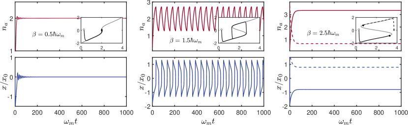
Figure S2: Time evolution of $x$ and $n_{\text{a}}$ is shown for different potential barrier heights: $\beta=0.5\hbar\omega_{m}$ (left), $\beta=1.5\hbar\omega_{m}$ (middle), and $\beta=2.5\hbar\omega_{m}$ (right), with the corresponding phase-space trajectories depicted in the insets. Other parameters remain the same as in Figure 2 of the main text.

Fig. S2 illustrates the dynamical behavior of the system, governed by Eq. (S14), for three distinct potential barrier heights denoted as $\beta$, as detailed in the main text. In the absence of a potential barrier, $x$ and $n_{\text{a}}$ exhibit rapid relaxation, ultimately converging to a fixed point in the phase space $(n_{\text{a}},x)$, as depicted in the left panel. As the potential barrier increases, $x$ and $n_{\text{a}}$ undergo periodic oscillations, corresponding to a limit cycle within the phase space, as shown in the middle panel. This represents the system alternating between two distinct steady states through self-sustained oscillations. When the potential barrier becomes excessively high, $x$ and $n_{\text{a}}$ once again undergo rapid relaxation but remain in one of the two fixed points, determined by the initial conditions, as illustrated in the right panel.

By conducting a stability analysis, we can delineate the boundaries of these three distinct dynamic regions within the parameter space $(g_{\kappa},\beta)$, which correspond to the thresholds at which self-sustained oscillations emerge. To accomplish this, we introduce small perturbations $(\delta_{n},\delta_{x})$ to the steady-state solutions $(n_{s},x_{s})$ of Equation (S14). Neglecting higher-order infinitesimals, we obtain the matrix equation

$$\partial_{t}\binom{\delta_{n}}{\delta_{x}}=\binom{-\kappa_{0}\,\,\,\kappa_{0}\partial_{x}\bar{n}_{\rm eff}(x_{s})}{-\frac{\hbar g_{\omega}}{m\gamma}\,\,\,-\frac{1}{m\gamma}\partial_{x}^{2}V(x_{s})}\binom{\delta_{n}}{\delta_{x}}.$$ (S16)

The steady solution is stable only when both eigenvalues of the coefficient matrix are non-positive.

In cases where the molecular damping is significantly larger, specifically $\gamma\gg\kappa_{0}$, the eigenvalues can be approximated as $\lambda_{1}\approx 0$ and $\lambda_{2}\approx-\frac{1}{m\gamma}\frac{\partial^{2}V(x_{s})}{\partial x^{2}}$. Consequently, the threshold values for stable $x_{s}$ are determined by the equation $\frac{\partial^{2}V(x_{s})}{\partial x^{2}}=0$, yielding two solutions: $x_{s}=x_{\pm}$. The boundary of the self-sustained oscillation region in the parameter space $(g_{\kappa},\beta)$, as depicted in Fig. 2 of the main text, can be established by substituting $x_{\pm}$ into Eq. (S14), which results in

$$\hbar g_{\omega}\bar{n}_{\rm eff}(x_{\pm})+\frac{\partial V(x_{\pm})}{\partial x}=0.$$ (S17)

III Thermodynamic Analysis

In our heat engine model, the cavity mode field serves as the working medium, while the reaction coordinates of the molecular switch represent the working degree of freedom. Thus, the effective Hamiltonian of the working medium is given by

$$\hat{H}_{\rm a}^{\rm eff}=\hbar(\omega_{\rm a}+g_{\omega}\hat{x})\hat{n}_{\rm a}.$$ (S18)

Based on the first law of thermodynamics and the definitions of work and heat within the framework of quantum thermodynamics, the instantaneous power output $\mathcal{P}$ of the heat engine is given by the sum of the heat exchange rates with the hot and cold reservoirs,

$$\mathcal{P}=\dot{Q}_{\rm h}+\dot{Q}_{\rm c}=\text{Tr}[\hat{H}_{\rm a}^{\rm eff}(\hat{\mathcal{L}}_{\rm h}+\hat{\mathcal{L}}_{\rm c})\rho].$$ (S19)

Using the master equation in Eq. (S11), we derive:

$$(\hat{\mathcal{L}}_{\rm h}+\hat{\mathcal{L}}_{\rm c})\rho=\dot{\rho}+\frac{i}{\hbar}[\hat{H}_{\rm om},\rho]-\hat{\mathcal{L}}_{\gamma}\rho.$$ (S20)

Substituting this into Eq. (S19), and utilizing the relationship $\hat{H}_{\rm om}=\hat{H}_{\rm a}^{\rm eff}+\hat{H}_{\rm m}$ along with the property of the Brownian dissipation superoperator, $\text{Tr}[\hat{H}_{\rm a}^{\rm eff}\hat{\mathcal{L}}_{\gamma}\rho]=0$, we obtain a revised expression for the power,

$$\mathcal{P} =\text{Tr}[\hat{H}_{\rm a}^{\rm eff}\dot{\rho}]+\frac{i}{\hbar}\langle[\hat{H}_{\rm a}^{\rm eff},\hat{H}_{\rm om}]\rangle$$ (S21)

$$=\frac{d\langle\hat{H}_{\rm a}^{\rm eff}\rangle}{dt}-\frac{\hbar g_{\omega}}{m}\langle\hat{n}_{\rm a}\hat{p}\rangle,$$

where the first term is the rate of change of internal energy, and the second term represents power done on the molecular switch. We show below that the first term does not contribute to average power and highlight differences in the second term between classical and quantum cases.

In the classical case, the operation of the heat engine is periodic, thus the average power is defined over a complete cycle,

$$P=\frac{1}{T}\oint\mathcal{P}\,dt,$$ (S22)

where the integral is taken over one cycle period $T$. Utilizing Eq. (S21) and disregarding quantum fluctuations and correlations, we obtain

$$P=\frac{1}{T}\oint\dot{H}_{\rm a}^{\rm eff}\,dt-\frac{1}{T}\frac{\hbar g_{\omega}}{m}\oint n_{\rm a}p\,dt,$$ (S23)

where the first term on the right-hand side disappears due to the periodic nature of energy changes. Notably, if we substitute $p=m\dot{x}$ and define $F=-\hbar g_{\omega}n_{\rm a}$, the second term takes the form of the power exerted by the radiation pressure force, $\frac{1}{T}\oint Fdx$.

In the quantum case, the system attains a steady state characterized by $\dot{\rho}_{\rm s}=0$. Consequently, the term representing the internal energy change in Eq. (S21) diminishes. Hence, the steady-state power is expressed as

$$\mathcal{P}_{s}=-\frac{\hbar g_{\omega}}{m}\langle\hat{n}_{\rm a}\hat{p}\rangle.$$ (S24)

Distinct from the classical case, the steady-state power in the quantum realm is influenced by the correlation between the cavity mode and the molecular switch. This component of the power, termed “correlation power” in the main text, can be measured by the difference

$$\Delta\mathcal{P}_{s}=-\frac{\hbar g_{\omega}}{m}(\langle\hat{n}_{\rm a}\hat{p}\rangle-\langle\hat{n}_{\rm a}\rangle\langle\hat{p}\rangle).$$ (S25)

IV Quasi-probability Picture

In the quantum case, the heat engine operates in a steady state, with continuous energy exchange between the cavity field and the molecule to maintain equilibrium. We can visualize these dynamics using quasi-probability distribution and flow fields in phase space.

The full phase space of the cavity-molecule coupled system is four-dimensional. However, a reduced phase space focusing on the amplitude of the cavity field and the molecule’s reaction coordinate is sufficient to capture the main quantum dynamics and enable comparisons with the classical case. Thus, we represent the quasi-probability distribution of the steady state $\rho_{s}$ using a modified Husimi-Q function based on the coherent state $|\alpha=re^{i\phi}\rangle$ with a phase integral and coordinate eigenstate $|x\rangle$, defined as

$$\tilde{\mathcal{Q}}(r,x)=\frac{1}{\pi}\int_{0}^{2\pi}\langle\alpha|\langle x|\rho_{\rm s}|x\rangle|\alpha\rangle rd\phi.$$ (S26)

In the case of overdamping, where $\gamma\gg\kappa_{0}$, the molecular switch adiabatically tracks the changes in the cavity mode and settles into the ground state $|g(n)\rangle$ of the effective potential $V(\hat{x})+\hbar g_{\omega}n\hat{x}$. Subsequently, the steady state of the system can be approximately expressed as

$$\rho_{s}\approx\sum_{n}P_{n}|n\rangle\langle n|\otimes|g(n)\rangle\langle g(n)|,$$ (S27)

where $|n\rangle$ denotes the number state of the cavity mode with a probability $P_{n}$. Given this, the term $[H_{\rm om},\rho_{s}]=0$, and the master equation for the steady state simplifies to

$$(\hat{\mathcal{L}}_{\rm h}+\hat{\mathcal{L}}_{\rm c}+\hat{\mathcal{L}}_{\gamma})\rho_{\rm s}=0.$$ (S28)

The superoperators $\hat{\mathcal{L}}_{\rm h,c}$ and $\hat{\mathcal{L}}_{\gamma}$ give rise to variations in the amplitude of the cavity field and the molecular displacement, respectively. These variations manifest as two non-zero time derivatives of the quasi-probability distribution, which are defined as

$$\tilde{D}(r,x) =\frac{1}{\pi}\int_{0}^{2\pi}\langle\alpha|\langle x|(\hat{\mathcal{L}}_{\rm h}\rho_{\rm s}+\hat{\mathcal{L}}_{\rm c}\rho_{\rm s})|x\rangle|\alpha\rangle rd\phi,$$ (S29)

$$\tilde{M}(r,x) =\frac{1}{\pi}\int_{0}^{2\pi}\langle\alpha|\langle x|\hat{\mathcal{L}}_{\rm\gamma}\rho_{\rm s}|x\rangle|\alpha\rangle rd\phi.$$

Given the steady state condition Eq. (S28), it follows that $\tilde{M}(r,x)=-\tilde{D}(r,x)$.

With these definitions, we can introduce a vector field $\vec{F}=(u,v)$ that delineates the quasi-probability flow within phase space $(r,x)$. The components of this vector field, $u(r^{\prime},x^{\prime})$ and $v(r^{\prime},x^{\prime})$, signify the flow density in the $r$ and $x$ dimensions, respectively, at any arbitrary position $(r^{\prime},x^{\prime})$ in phase space. These components are expressed through the integrals of $\tilde{D}(r,x)$ along the $r$-dimension and $\tilde{M}(r,x)$ along the $x$-dimension, respectively, as follows

$$u(r^{\prime},x^{\prime}) =-\int_{0}^{r^{\prime}}\tilde{D}(r,x^{\prime})\,dr,$$ (S30)

$$v(r^{\prime},x^{\prime}) =-\int_{-\infty}^{x^{\prime}}\tilde{M}(r^{\prime},x)\,dx=\int_{-\infty}^{x^{\prime}}\tilde{D}(r^{\prime},x)\,dx.$$

Note that a key feature of this quasi-probability flow field is its zero divergence,

$$\nabla\cdot\vec{F}=\partial_{r}u(r,x)+\partial_{x}v(r,x)=0,$$ (S31)

reflecting the conservation of probability, i.e., ${\rm Tr}\rho_{\rm s}=1$.