Efficient Data-Driven Leverage Score Sampling Algorithm for the Minimum Volume Covering Ellipsoid Problem in Big Data
Abstract
The Minimum Volume Covering Ellipsoid (MVCE) problem, characterised by observations in dimensions where , can be computationally very expensive in the big data regime. We apply methods from randomised numerical linear algebra to develop a data-driven leverage score sampling algorithm for solving MVCE, and establish theoretical error bounds and a convergence guarantee. Assuming the leverage scores follow a power law decay, we show that the computational complexity of computing the approximation for MVCE is reduced from to , which is a significant improvement in big data problems. Numerical experiments demonstrate the efficacy of our new algorithm, showing that it substantially reduces computation time and yields near-optimal solutions.
1 Introduction
The Minimum Volume Covering Ellipsoid (MVCE) problem arises in many applied and theoretical areas. Statistical applications include outlier detection [33], clustering [26], and the closely related D-optimal design problem [30]. In fact, the MVCE problem and the D-optimal design problem are dual to one another [29, 32]. Containing ellipsoids are used in parameter identification and control theory to describe uncertainty sets for parameters and state vectors [4, 28]. Minimum volume covering ellipsoids are also used in computational geometry and computer graphics [10], in particular, for collision detection [3].
Many algorithms for computing MVCEs and D-optimal designs have been studied in the literature. These include Frank-Wolfe type algorithms [13, 37, 1, 17, 20], interior point algorithms [18, 22], the Dual Reduced Newton algorithm [31], the Cocktail algorithm [39], the Randomised Exchange algorithm [14], and the Fixed Point algorithm [5, 38]. However, when these algorithms are applied to very large datasets, they may be computationally inefficient, and may exceed storage limitations [14]. One solution is to combine such solution algorithms with active set or batching strategies [31, 16, 19, 25]. The main idea of this approach is to iteratively apply the solution algorithm to a smaller subset of points until convergence to the solution. The motivation for this approach is that an ellipsoid is only determined by at most points on its boundary [15].
Instead of applying an active set strategy, we apply deterministic sampling to reduce the number of points considered by the algorithm. This deterministic sampling method selects points corresponding to the highest statistical leverage scores. The resulting compressed dataset approximately maintains many of the qualities of the original dataset, provided that the number of samples is sufficiently large [24, 21]. However, there is no immediate guarantee of the quality of solution to the MVCE problem for this compressed dataset. In this paper, we provide the first theoretical guarantees on the quality of initial and final solution for the MVCE problem for this deterministic sampling method. In numerical experiments, we apply the MVCE algorithm to just our sampled data. Our experiments show that this sampling method greatly improves computation time, and provides near-optimal final solutions.
For the remainder of Section 1, we outline the contributions and limitations of our approach. In Sections 2 and 3, we formally introduce the MVCE problem, and leverage score based sampling, respectively. Our approach is presented in Section 4, and our theoretical results in Sections 5 and 6. In Section 7, we show our numerical results. We present our conclusions in Section 8. Some proofs are provided in Appendices A, B, C, D, and additional numerical results are presented in Appendix E.
1.1 Contributions
In this paper, we present a new simplified proof of Theorem 1 in [21]. Using this theorem, we provide the first theoretical guarantees on the quality of initial and final solution for the MVCE problem when using deterministic leverage score sampling. Further, we show that these guarantees still hold (with high probability) when approximate leverage scores are used.
Assuming a power law decay on the leverage scores, we show that our method improves the theoretical computation time required to approximate the MVCE. We also demonstrate the efficiency of our approach on synthetic and real world datasets.
1.2 Limitations
We require the leverage scores to follow a power law decay, so that our sample size is guaranteed to be much smaller than . However, in our numerical experiments, we demonstrate that this requirement can usually be relaxed in practice. In future work, we aim to remove the power law decay requirement.
We also assume . This is because our base algorithm, the Wolfe-Atwood (WA) algorithm [37, 1], performs best under this assumption. However, if this condition is violated, we can use a different underlying algorithm which performs well when and are of similar order (e.g., the Fixed Point algorithm [5, 38]).
Finally, we make no assumption on the sparsity of our data matrix . Although this gives wider applicability, it means we do not take advantage of any sparse input. Again, this can be resolved by using a different underlying algorithm (e.g., the Fixed Point algorithm [5, 38]).
Notation.
Throughout this paper, vectors and matrices are denoted by bold lowercase and bold uppercase letters, respectively (e.g. and ). The th entry of is denoted , and the th entry of is denoted . Let and be symmetric positive definite matrices, then if is symmetric positive semidefinite; and if is symmetric positive definite. The determinant of a matrix is denoted . Unless otherwise specified, . We use regular lowercase to denote scalar constants (e.g. ). Finally, denotes a vector of ones, and denotes the vector with one at position , and zero otherwise.
2 The minimum volume covering ellipsoid problem
Let be a set of data points in . Then the minimum volume covering ellipsoid is the ellipsoid that covers , which attains the minimum volume of all covering ellipsoids of . We assume throughout that there exists a non-degenerate minimum volume covering ellipsoid.
We define the ellipsoid as
where is the centre of the ellipsoid, and is an -dimensional symmetric positive definite matrix. Its volume is given by
where is the volume of the unit ball in (e.g., see [34]).
We can now write the mathematical formulation of the Minimum Volume Covering Ellipsoid problem. Suppose we have a finite set of points . Then its minimum volume covering ellipsoid can be found by solving
| (P0) | ||||
| subject to |
Although the objective function is convex, (P0) itself is not convex [34].
We therefore reformulate (P0) so that it is convex. At the cost of working in , we can calculate the centred minimum volume covering ellipsoid, and recover the solution to (P0) [32]. Therefore, we can set , and obtain
| (P) | ||||
| subject to |
We let denote an optimal solution to Problem (P). Then MVCE is the minimum volume covering ellipsoid. We will refer to Problem (P) as the MVCE problem.
The dual problem to Problem (P) is the D-optimal design problem. This problem is concave, and can be formulated as
| (D) | ||||
| subject to |
where is called the design vector. We note that for every design vector , we can find its associated shape matrix
provided that the inverse exists. Hence if we have an optimal solution to Problem (D), then the optimal solution to Problem (P) is .
We note that Problem (D) (and Problem (P)) cannot usually be solved exactly, so we will focus on deriving approximate solutions. To ensure the chosen algorithm terminates with a guaranteed quality of solution, we will define some approximate optimality conditions. A feasible for Problem (D) is called -primal feasible if satisfies
for all . If additionally satisfies
for all , then we say that is -approximately optimal. These optimality conditions ensure the optimality gap is small.
3 Sampling using leverage scores
The concept of statistical leverage scores has long been used in statistical regression diagnostics to identify outliers [27]. Given a data matrix with , consider any orthogonal matrix such that . The th leverage score corresponding to the th row of is defined as
It can be easily shown that this is well defined in that the leverage score does not depend on the particular choice of the basis matrix . Furthermore, the th leverage score is the th diagonal entry of the hat matrix, that is,
where
The hat matrix is symmetric and idempotent. We can use these properties to easily show that
for all , and
We only consider full rank matrices, , that is, with . Thus
3.1 Deterministic sampling
When sampling deterministically, we sample the rows from with highest leverage scores. Without loss of generality, assume that the leverage scores are ordered . We summarise the sampling procedure in Algorithm 1.
We note that is carefully chosen, to ensure the following subspace embedding result.
Algorithm 1 has time complexity , due to the cost of calculating the leverage scores exactly. This can be improved by using approximate leverage score algorithms. Drineas et al. [8] developed a fast sampled randomised Hadamard transform (SRHT) with time complexity . More recently, Eshragh et al. [11] developed the Sequential Approximate Leverage-Score Algorithm (SALSA) with time complexity . Moreover, we can use these approximate leverage score algorithms to prove an analogous result to Theorem 3.1 (see Appendix B).
4 Our approach
We are interested in calculating MVCE, where , . For very large (and ), this can be very computationally expensive. Instead of calculating MVCE directly, we will calculate the MVCE on a much smaller subset of . We select our subset by using leverage score based sampling, as introduced in Section 3. Let this subset be , where contains up to points sampled from . For ease of calculation, let the points from be stored in the rows of the data matrix . Then we sample rows from , which we store in the rows of . We then use instead of in our solution algorithm. That is, our solution algorithm solves the concave problem
| (Ds) | ||||
| subject to |
4.1 Computational complexity
We compare the computational complexity of our algorithm to the current state of the art algorithm, the Wolfe-Atwood (WA) algorithm [37, 1], which computes a -approximately optimal solution to (D). It uses the Kumar-Yildirim (KY) initialisation [20], which places equal weight on a small subset of points. These algorithms have time complexity [36] and [20], respectively. Together, this costs .
The computational complexity of our approach is as follows. We calculate approximate leverage scores in time, which, with high probability, satisfy , for some [11]. Then Algorithm 1 also runs in time. We then use the WA algorithm with KY initialisation to find an optimal solution to (Ds). Since , these algorithms have time complexity and , respectively. Thus, the total time complexity is . Further, if the leverage scores exhibit a power law decay, then (see Appendix B).
4.2 Comparison with the work of Cohen et. al.
Recently, Cohen et. al. [5] developed the Fixed Point algorithm, which computes a -primal feasible solution to (D). Woodruff and Yasuda [38] extend this result; by sampling rows of with probabilities proportionate to the weights calculated by the Fixed Point algorithm, they obtain a -approximately optimal solution to (D).
The computational complexity of the Fixed Point algorithm is as follows. We examine Algorithm 2 from [5], which uses sketching techniques from randomised numerical linear algebra to speed up each iteration. Theorem C.7 from [5] states that Algorithm 2 takes at most iterations to complete. In each iteration there are linear systems of the form to be solved. Assuming is dense, solving each of these linear systems costs . This gives a total time complexity of for dense matrices.
In big data regimes with , it is reasonable to assume that is desirable. This assumption holds for many problem instances considered in the MVCE literature, since these problems typically have dimension , and are solved until tolerance (or stricter) is achieved (see, e.g. [31, 7, 39, 16, 19]). With this assumption, Algorithm 2 has total time complexity and our algorithm has total time complexity , where . Thus, in the context of tall data matrices with dense input, our algorithm outperforms the Fixed Point algorithm theoretically. (This also holds numerically, see Appendix E.1.)
5 Initial optimality gap
We would like to know how well MVCE approximates MVCE. We will first provide an upper bound for the initial optimality gap, for a particular choice of initial . This must be feasible for Problem (Ds), that is, we must have , and . We choose
Then the initial optimality gap is given by
where is the optimal objective value when the full set is considered.
To derive our bound, we will compare our initial solution with an initialisation due to Khachiyan [17]. Khachiyan’s initialisation puts equal weight on all points of , and guarantees that
as shown by Khachiyan [17]. Therefore, our bound can be found by exploiting the fact that
Upon simplification,
| (1) |
and, similarly,
| (2) |
Hence
| (3) |
This suggests the need to compare with .
Suppose we construct as in Algorithm 1. Then Theorem 3.1 guarantees that
Now, for positive semidefinite matrices , , with , we have
| (4) |
Since the logarithm is monotonic, it then follows that . Hence
| (5) |
Combining Equations (3) and (5), we obtain the bound presented in Theorem 5.1.
Theorem 5.1.
Select using Algorithm 1, and let our initial solution be given by . Then
Proof.
See Appendix C. ∎
6 Final optimality gap
We now provide an upper bound for the final optimality gap. The final optimality gap is given by
where is the optimal objective value when only is considered. Note that for any feasible for (Ds), we have
since is concave.
Consider the feasible solution for (Ds), given by
where contains the first entries of . We would like a bound similar to the one in Theorem 3.1, with replaced with a rescaled version . More precisely, let
To apply Theorem 3.1, we require
for some . The strategy is to show that
| (6) |
which is less than by construction of Algorithm 1. Therefore, we may apply Theorem 3.1 with instead of , to obtain the bound
That is, the feasible solution satisfies
Hence
Theorem 6.1.
Proof.
See Appendix D. ∎
7 Numerical results
We generate three large datasets of size , . Without loss of generality, we assume the leverage scores are sorted in descending order, that is, . The first dataset is Rotated Cauchy [34]. The points are generated so that they have rotational symmetry, and the distances of the points from the origin are Cauchy. The leverage scores of these points quickly decay. The second dataset is Lognormal, which has a shallower leverage score decay. The third dataset is Gaussian, which has leverage scores that are close to uniform. We provide additional numerical results in Appendix E.
All computations are performed on a personal laptop with a 64 bit MacOS 13 operating system, and a 2.4 GHz Quad-Core Intel Core i5 processor with 8 GB of RAM. The algorithms are run using MATLAB (R2021a).
We use the WA algorithm [37, 1] to calculate the MVCEs of the two datasets, with . We initialise using the KY algorithm [20]. We use Todd’s Matlab implementation of these algorithms [35]. Then, for varying from to 10 of , we sample from each dataset in three ways: deterministic leverage score sampling, uniform sampling, and randomised leverage score sampling (sampling with probabilities proportionate to the leverage scores [9]). In these results, we use the exact leverage scores.
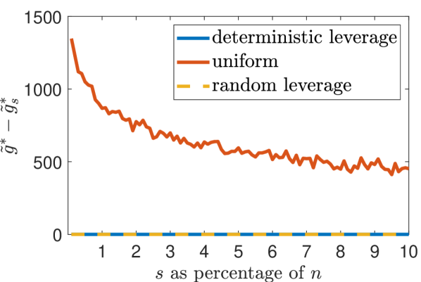
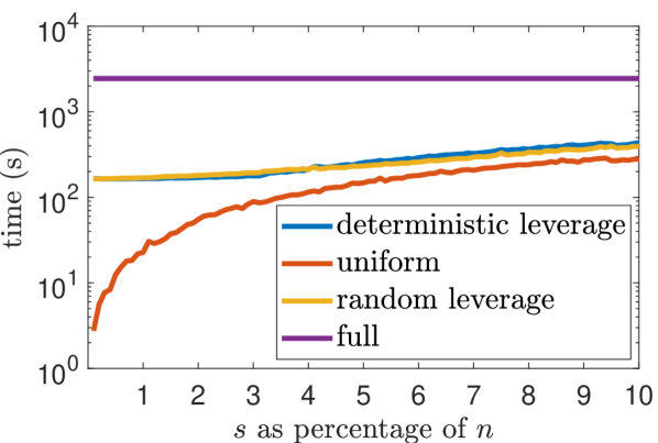
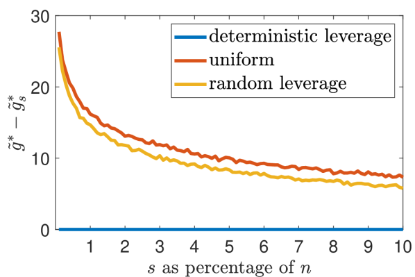
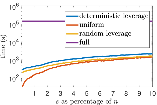
Let and be the optimal values obtained when using the WA algorithm on the full and sampled datasets respectively. In Figure 1(a), we summarise the calculated optimality gaps for the Rotated Cauchy dataset. The deterministic and randomised leverage score sampling performed similarly, with near zero optimality gap for all values of . Uniform sampling performed poorly, its optimality gap decreasing with increasing . In Figure 1(b) we summarise the total computation time for calculating the MVCEs. For the sampled datasets, this also includes the computation time for calculating leverage scores (if applicable), and sampling from the dataset. The total computation time for the full dataset was seconds, that is, just over minutes. Uniform sampling was faster than the leverage score sampling methods (due to the calculation of the leverage scores), but had very large optimality gaps (see Figure 1(a)).
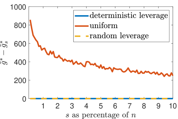
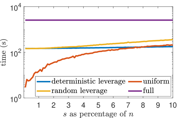
In Figure 2(a), we summarise the calculated optimality gaps for the Lognormal dataset. The deterministic and randomised leverage score sampling performed similarly, with zero optimality gap for all values of . Uniform sampling performed poorly, its optimality gap decreasing with increasing . In Figure 2(b) we summarise the total computation time for calculating the MVCEs. The total computation time for the full dataset was seconds, that is, just over minutes. Uniform sampling was generally faster than the leverage score sampling methods (due to the calculation of the leverage scores), but had very large optimality gaps (see Figure 2(a)).
In Figure 3(a), we summarise the calculated optimality gaps for the Gaussian dataset. Only the deterministic leverage score sampling performed well, with near zero optimality gap for all . The uniform and randomised leverage score sampling performed similarly, with optimality gaps decreasing with increasing . This is unsurprising, since the leverage scores for a Gaussian dataset are close to uniform. In Figure 3(b) we summarise the total computation time for calculating the MVCEs. The total computation time for the full dataset was very large, at seconds, that is, over hours. As with the other dataset, uniform sampling was the fastest, but at the cost of a larger optimality gap (see Figure 3(a)). Additionally, both leverage score sampling methods had similar runtimes, but only the deterministic sampling had near zero optimality gap (see Figure 3(a)).
Overall, the deterministic leverage score sampling performs the best, achieving both a small optimality gap and greatly decreasing computation time on all three datasets.
8 Conclusion
In this paper, we have provided the first theoretical guarantees on the quality of initial and final solutions for the MVCE problem, when sampling points deterministically according to their statistical leverage scores. We proved this approach is efficient, assuming the leverage scores exhibit a power law decay. Numerical results show that our data-driven leverage score sampling algorithm performs even better than the established theoretical error bounds, even in cases where the leverage scores are close to uniform distribution, which could be a by-product of our analysis. Future work could include extending these results to other data-driven sampling methods, including randomised leverage score sampling, and also implementing this algorithm extensively on real-world large-scale datasets.
References
- [1] Corwin L. Atwood. Sequences converging to D-optimal designs of experiments. The Annals of Statistics, 1(2):342–352, 1973.
- [2] Rajen Bhatt and Abhinav Dhall. Skin Segmentation. UCI Machine Learning Repository, 2012. DOI: https://doi.org/10.24432/C5T30C. License: CC BY 4.0.
- [3] Yu-Jen Chen, Ming-Yi Ju, and Kao-Shing Hwang. A virtual torque-based approach to kinematic control of redundant manipulators. IEEE Transactions on Industrial Electronics, 64(2):1728–1736, 2016.
- [4] F. L. Chernousko. Ellipsoidal state estimation for dynamical systems. Nonlinear Analysis: Theory, Methods & Applications, 63(5-7):872–879, 2005.
- [5] Michael B Cohen, Ben Cousins, Yin Tat Lee, and Xin Yang. A near-optimal algorithm for approximating the John ellipsoid. In Conference on Learning Theory, pages 849–873. PMLR, 2019.
- [6] Michael B. Cohen, Yin Tat Lee, Cameron Musco, Christopher Musco, Richard Peng, and Aaron Sidford. Uniform sampling for matrix approximation. In Proceedings of the 2015 Conference on Innovations in Theoretical Computer Science, pages 181–190, 2015.
- [7] S Damla Ahipasaoglu, Peng Sun, and Michael J Todd. Linear convergence of a modified Frank–Wolfe algorithm for computing minimum-volume enclosing ellipsoids. Optimisation Methods and Software, 23(1):5–19, 2008.
- [8] P. Drineas, M. Magdon-Ismail, M.W. Mahoney, and D.P. Woodruff. Fast approximation of matrix coherence and statistical leverage. Journal of Machine Learning Research, 13(Dec):3475–3506, 2012.
- [9] Petros Drineas, Michael W. Mahoney, and Shan Muthukrishnan. Relative-error CUR matrix decompositions. SIAM Journal on Matrix Analysis and Applications, 30(2):844–881, 2008.
- [10] David Eberly. 3D game engine design: a practical approach to real-time computer graphics. CRC Press, 2006.
- [11] Ali Eshragh, Luke Yerbury, Asef Nazari, Fred Roosta, and Michael W. Mahoney. SALSA: Sequential approximate leverage-score algorithm with application in analyzing big time series data. arXiv preprint arXiv:2401.00122, 2023.
- [12] Jordi Fonollosa. Gas sensor array under dynamic gas mixtures. UCI Machine Learning Repository, 2015. DOI: https://doi.org/10.24432/C5WP4C. License: CC BY 4.0.
- [13] Marguerite Frank, Philip Wolfe, et al. An algorithm for quadratic programming. Naval research logistics quarterly, 3(1-2):95–110, 1956.
- [14] Radoslav Harman, Lenka Filová, and Peter Richtárik. A randomized exchange algorithm for computing optimal approximate designs of experiments. Journal of the American Statistical Association, 115(529):348–361, 2020.
- [15] Fritz John. Extremum problems with inequalities as subsidiary conditions. In Traces and Emergence of Nonlinear Programming, pages 197–215. Springer Basel, 2014.
- [16] Linus Källberg and Daniel Andrén. Active set strategies for the computation of minimum-volume enclosing ellipsoids. Technical report, Mälardalen Real-Time Research Centre, Mälardalen University, November 2019.
- [17] Leonid G. Khachiyan. Rounding of polytopes in the real number model of computation. Mathematics of Operations Research, 21(2):307–320, 1996.
- [18] Leonid G. Khachiyan and Michael J. Todd. On the complexity of approximating the maximal inscribed ellipsoid for a polytope. Mathematical Programming, 61(1-3):137–159, 1993.
- [19] Jakub Kudela. Minimum-volume covering ellipsoids: Improving the efficiency of the Wolfe-Atwood algorithm for large-scale instances by pooling and batching. In MENDEL, volume 25, pages 19–26, 2019.
- [20] Piyush Kumar and E. Alper Yildirim. Minimum-volume enclosing ellipsoids and core sets. Journal of Optimization Theory and applications, 126(1):1–21, 2005.
- [21] Shannon R McCurdy, Vasilis Ntranos, and Lior Pachter. Deterministic column subset selection for single-cell rna-seq. Plos one, 14(1):e0210571, 2019.
- [22] Yurii Nesterov and Arkadii Nemirovskii. Interior-point polynomial algorithms in convex programming. SIAM, 1994.
- [23] Bruno Ordozgoiti, Antonis Matakos, and Aristides Gionis. Generalized leverage scores: Geometric interpretation and applications. In International Conference on Machine Learning, pages 17056–17070. PMLR, 2022.
- [24] Dimitris Papailiopoulos, Anastasios Kyrillidis, and Christos Boutsidis. Provable deterministic leverage score sampling. In Proceedings of the 20th ACM SIGKDD international conference on Knowledge discovery and data mining, pages 997–1006, 2014.
- [25] Samuel Rosa and Radoslav Harman. Computing minimum-volume enclosing ellipsoids for large datasets. Computational Statistics & Data Analysis, 171:107452, 2022.
- [26] Judah Ben Rosen. Pattern separation by convex programming. Journal of Mathematical Analysis and Applications, 10(1):123–134, 1965.
- [27] Peter J. Rousseeuw and Mia Hubert. Robust statistics for outlier detection. Wiley interdisciplinary reviews: Data mining and knowledge discovery, 1(1):73–79, 2011.
- [28] Fred Schweppe. Recursive state estimation: Unknown but bounded errors and system inputs. IEEE Transactions on Automatic Control, 13(1):22–28, 1968.
- [29] R. Sibson. Discussion of Dr Wynn’s and of Dr Laycock’s papers. Journal of the Royal Statistical Society: Series B (Methodological), 34(2):181–183, 1972.
- [30] S. D. Silvey. Optimal design: and introduction to the theory for parameter estimation. London, Chapman and Hall/CRC, 1980.
- [31] Peng Sun and Robert M. Freund. Computation of minimum-volume covering ellipsoids. Operations Research, 52(5):690–706, 2004.
- [32] D. M. Titterington. Optimal design: some geometrical aspects of D-optimality. Biometrika, 62(2):313–320, 1975.
- [33] D. M. Titterington. Estimation of correlation coefficients by ellipsoidal trimming. Journal of the Royal Statistical Society: Series C (Applied Statistics), 27(3):227–234, 1978.
- [34] Michael J. Todd. Minimum-volume ellipsoids: Theory and algorithms. SIAM, 2016.
- [35] Michael J. Todd. Minvol. SIAM, 2016. URL: http://archive.siam.org/books/mo23/.
- [36] Michael J. Todd and E. Alper Yıldırım. On Khachiyan’s algorithm for the computation of minimum-volume enclosing ellipsoids. Discrete Applied Mathematics, 155(13):1731–1744, 2007.
- [37] Philip Wolfe. Convergence theory in nonlinear programming. Integer and nonlinear programming, pages 1–36, 1970.
- [38] David P Woodruff and Taisuke Yasuda. New subset selection algorithms for low rank approximation: Offline and online. In Proceedings of the 55th Annual ACM Symposium on Theory of Computing, pages 1802–1813, 2023.
- [39] Yaming Yu. D-optimal designs via a cocktail algorithm. Statistics and Computing, 21(4):475–481, 2011.
Appendix A Alternative proof for Theorem 3.1
We provide a proof of Theorem 3.1, including a new simplified proof of the lower bound.
Theorem A.1.
Let Suppose the rows of are ordered such that , for some . Let contain the first rows of . Then
Proof.
We consider the upper bound first. For any sampling matrix , we have that
Now, the conjugation rule states that if and are symmetric positive semidefinite matrices with , and is any real matrix of compatible dimension, then . Using this, we obtain
which rearranges to give our upper bound.
We now prove the lower bound. We will use the fact that for any ,
see, for example, the proof of Lemma 4 in [6]. Hence
since . Rearranging, we obtain our lower bound. ∎
Appendix B Deterministic approximate leverage score sampling
The computation time in Algorithm 1 is dominated by the cost of calculating the leverage scores exactly, which is . We can instead use approximate leverage scores, which are more computationally efficient to calculate. We demonstrate the approach using the algorithm of Eshragh et al. [11].
Theorem B.1 ([11], Theorem 4).
Fix a constant . Let the leverage scores of the rows of a matrix be given by . Then there exists a randomised algorithm that calculates approximate leverage scores such that with high probability, simultaneously for all , . This algorithm has time complexity .
We then sample deterministically according to these approximate leverage scores. We summarise the modified sampling procedure in Algorithm 2. For simplicity, assume we can write , for some .
We have chosen carefully, to ensure the following subspace embedding result.
Corollary B.2.
Let , and . Use Algorithm 2 to construct . Then, with high probability, we have
Proof.
For this proof, we only need to show that holds with high probability. We can then apply Theorem A.1 to obtain our bound.
Assume that holds simultaneously for all . By construction of Algorithm 2, we have
Then since , for all , we have
that is,
∎
Corollary B.3.
If the leverage scores exhibit a power law decay, then .
Appendix C Missing details in proof of Theorem 5.1
C.1 Proof of Equations (1) and (2)
We have that
and, similarly,
C.2 Proof of Inequality (4)
We first need to prove the following lemma.
Lemma C.1.
Suppose we have two symmetric positive semidefinite matrices and , with . Let the eigenvalues of be given by , and the eigenvalues of be given by . Then for all , we have
Proof.
Use Min-max Theorem, along with the fact that for all . ∎
We are now ready to prove the inequality.
Lemma C.2.
Suppose we have two symmetric positive semidefinite matrices and , with . Then
Proof.
We have that
where the inequality uses Lemma C.1 and the fact that is a monotonically increasing function. Then
where the inequality is because the exponential function is monotonically increasing. ∎
Appendix D Final optimality gap
We break this proof into two cases:
-
1.
, for all , and
-
2.
, for all .
We do this because the proof of Inequality (6) relies on scaling so that the first diagonal terms are , and the last diagonal terms are . Having any zeros in the first terms prevents such a scaling.
We consider Case 1 first. First, follow the proof outline from Section 6. Then, what remains to be shown is that Inequality (6) holds.
D.1 Case 1: for all
The following lemma will be useful for proving Inequality (6). It shows the change in leverage scores when one row of is scaled.
Lemma D.1 ([23], Lemma 3.2).
Let have rank . Let . Define as the diagonal matrix satisfying , , if . Then
and, in particular,
We now ready to prove the inequality.
Proposition D.2.
Proof.
The structure of this proof is based on the proof of Theorem 3.2 in [23]. We will show that the sum of the last leverage scores of do not increase when we premultiply it by . Without loss of generality, we assume that . This is because, for any , we can write
where , such that is sufficiently small.
First, we scale so that the first diagonal terms are , and the last diagonal terms are . Let . We define
We exploit the fact that
To see how affects the leverage scores of , we will consider scaling each row separately. We define as the diagonal matrix satisfying and , if . Now, we consider the leverage scores of . From Lemma D.1, we have
-
1.
If , then . Hence , and if .
-
2.
If , then . Hence , and if .
Now, we consider scaling the first rows. From the previous discussion, we can conclude that the leverage scores of the last rows do not increase. Therefore, the sum of the first leverage scores does not decrease. (This is because the sum of the leverage scores remains constant, since scaling rows by non-zero constants does not affect the rank.) Next, consider scaling the last rows. From the discussion above, all the leverage scores of the first rows cannot decrease. That is, the sum of the first leverage scores again does not decrease. We conclude that the sum of the last leverage scores cannot increase. (This is because the sum of the leverage scores remains constant. Suppose . Then , which is a contradiction, since is invertible.) Hence
∎
D.2 Case 2: for all
This time, we will examine a -feasible solution for (D), which has for all . Such a solution can be achieved by using the Frank-Wolfe algorithm [13, 37] with Khachiyan’s initialisation [17].
Consider the feasible solution for (Ds), given by
where contains the first entries of . We would like a bound similar to the one in Theorem A.1, with replaced with
We require the following result.
Proof.
Follow the proof of Proposition D.2, but replace with , and redefine . ∎
Then, by the construction of Algorithm 1, we have
for some . Therefore, we may apply Theorem A.1 with instead of , to obtain the bound
That is, the feasible solution satisfies
We are now ready to prove the final optimality gap.
Appendix E More numerical results
E.1 Comparison of our algorithm with the Fixed Point algorithm
All computations in this section are performed on a personal laptop with a 64 bit Windows 11 Home operating system (Version 23H2), and a 3.30 GHz 11th Gen Intel Core i7-11370H processor with 40 GB of RAM. The algorithms are run using MATLAB (R2021a).
In this subsection, we compare our algorithm to the Fixed Point algorithm [5]. For consistency, we run our algorithm using of . We run both algorithms on Gaussian datasets of size , with dimension ranging from 2 to 10. Table 1 summarises the total computation time required for both algorithms, for varying values of accuracy parameter .
| Time (s) | ||||
|---|---|---|---|---|
| Our algorithm | Fixed Point algorithm | |||
| 2 | 0.0914 0.0220 | 1.4331 0.0877 | ||
| 0.0922 0.0210 | 12.1627 0.8764 | |||
| 0.0873 0.0215 | 63.1388 6.2418 | |||
| 5 | 0.1330 0.0219 | 3.6558 0.2074 | ||
| 0.1956 0.0442 | 12.1783 1.3380 | |||
| 0.2125 0.0390 | 47.2873 11.6625 | |||
| 10 | 0.2483 0.0618 | 6.0298 0.7460 | ||
| 0.4177 0.1025 | 21.8280 3.9056 | |||
| 0.4313 0.1077 | 117.9867 41.5669 | |||
We now apply the same methods to Gaussian matrices of dimension , with varying number of points and accuracy parameter . Table 2 summarises the total computation time required for both algorithms.
| Time (s) | |||||
|---|---|---|---|---|---|
| runs | Our algorithm | Fixed Point algorithm | |||
| 100 | 100 | 0.0927 0.0402 | 0.7270 0.1886 | ||
| 100 | 0.2578 0.1991 | 5.6216 1.5382 | |||
| 100 | 0.3013 0.0833 | 18.6236 4.8307 | |||
| 50 | 0.5162 0.1292 | 82.4097 26.7802 | |||
| 20 | 1.9359 0.1371 | 160.1398 34.8062 | |||
| 1 | 101.0625 | 4837.5313 | |||
In both Tables 1 and 2, we notice that as increases, the time taken for both methods generally increases. However, the increase in time for our algorithm is minimal, while the increase in time for the Fixed Point algorithm is significant. In the final row of Table 2, our algorithm takes less than 2 minutes, compared with the Fixed Point algorithm, which took about 80 minutes.
We emphasise that the examples considered here are smaller than those we considered in Section 7, and the accuracy parameter is much larger than our desired . Regardless, we ran the Fixed Point algorithm on the examples from Section 7. We found that for all three datasets, the algorithm did not converge in two hours of runtime.
E.2 Real world data
All computations in this section are performed on a personal laptop with a 64 bit MacOS 13 operating system, and a 2.4 GHz Quad-Core Intel Core i5 processor with 8 GB of RAM. The algorithms are run using MATLAB (R2021a).
We now test our algorithm on three smaller datasets from the UCI Machine Learning Repository. Table 3 summarises the size of each dataset, and time to compute the MVCE using the WA algorithm [37, 1].
| Dataset | Time (s) | ||
|---|---|---|---|
| Ethylene CO [12] | 19 | 85.92 0.17 | |
| Ethylene CH4 [12] | 19 | 75.89 0.38 | |
| Skin [2] | 4 | 0.54 0.04 |
We then apply our algorithm on each dataset, varying sample size from 1 to 10 of . In Table 4, we summarise the optimality gaps. The deterministic sampling performed well on all datasets, achieving very small optimality gaps when is 10 of . In Table 5, we summarise the computation times. Although the deterministic sampling was the slowest, all sampling methods decreased the total computation time required to calculate the MVCE.
| Optimality Gap | ||||
|---|---|---|---|---|
| Dataset | det | prob | unif | |
| Ethylene CO [12] | 1 | 4.66 | 1.01 0.11 | 5.47 0.65 |
| 5 | 0.02 | 0.43 0.03 | 4.40 1.03 | |
| 10 | 5.67E-06 | 0.25 0.04 | 3.24 0.48 | |
| Ethylene CH4 [12] | 1 | 1.59 | 1.48 0.09 | 3.53 0.42 |
| 5 | 0.05 | 0.66 0.05 | 1.69 0.15 | |
| 10 | 0.01 | 0.37 0.08 | 1.35 0.11 | |
| Skin [2] | 1 | 0.75 | 0.07 0.02 | 0.25 0.13 |
| 5 | 0.56 | 0.02 0.01 | 0.05 0.03 | |
| 10 | -3.55E-15 | 0.03 0.01 | 0.04 0.02 | |
| Time (s) | ||||
|---|---|---|---|---|
| Dataset | det | prob | unif | |
| Ethylene CO [12] | 1 | 6.00 0.12 | 5.42 0.74 | 4.01 0.39 |
| 5 | 15.00 0.56 | 9.94 0.47 | 7.55 0.05 | |
| 10 | 15.71 0.14 | 14.32 1.26 | 11.66 0.95 | |
| Ethylene CH4 [12] | 1 | 5.91 0.30 | 5.24 0.36 | 3.35 0.30 |
| 5 | 13.56 0.58 | 10.00 1.10 | 7.95 1.08 | |
| 10 | 15.18 0.34 | 13.05 0.81 | 10.26 0.93 | |
| Skin [2] | 1 | 0.04 0.01 | 0.04 0.01 | 0.05 0.03 |
| 5 | 0.15 0.03 | 0.13 0.01 | 0.10 0.02 | |
| 10 | 0.15 0.03 | 0.17 0.03 | 0.13 0.02 | |