Structure factor and topological bound of twisted bilayer semiconductors
at fractional fillings

Abstract

The structure factor is a useful observable for probing charge density correlations in real materials, and its long-wavelength behavior encapsulated by “quantum weight” has recently gained prominence in the study of quantum geometry and topological phases of matter. Here we employ the static structure factor, $S(\mathbf{q})$, to explore the phase diagram of twisted transition metal dichalcogenides (TMDs), specifically $t$MoTe₂, at a filling factors $\nu=1/3$, $2/3$ under varying displacement fields. Our results reveal a topological phase transition between a fractional Chern insulator (FCI) and a generalized Wigner crystal (GWC). This transition is marked by the appearance of Bragg peaks at charge-density-wave vectors, and simultaneously, large decrease of $S(\mathbf{q})$ at small $\mathbf{q}$ which lowers the interaction energy. We further calculate the quantum weight of various FCI states, verifying the universal topological bound. Our findings provide new insights into the phase diagram of twisted TMDs and establish a general framework for characterizing topological phases through structure factor analysis.

Introduction—. The structure factor is a fundamental quantity for probing crystal structure and charge/spin density fluctuations in real materials, which can be measured by X-ray diffraction, electron loss spectroscopy and neutron scattering. In particular, the static (or equal-time) structure factor $S(\mathbf{q})$ is a ground state property defined as the Fourier transform of spatial density correlation. In periodic solids, Bragg peaks in the structure factor identify crystal structures and charge density wave orders [1]. In quantum liquids, the static structure factor encodes useful information about the ground state and excitation spectrum [2]. For example, the structure factor of helium exhibits a characteristic peak at the wavevector set by the inverse particle distance, which is closely related to the roton excitation [3].

Recently, the behavior of the structure factor $S(\mathbf{q})$ at small $\mathbf{q}$, which characterizes long-wavelength density correlations, has received growing attention. For gapped many-body systems, $S(\mathbf{q}\rightarrow 0)$ is generally quadratic in $\mathbf{q}$ and the quadratic coefficient $K$ defines a fundamental ground state property recently termed quantum weight [4, 5]. Interestingly, quantum weight is directly related to optical response [5], charge fluctuation [6, 7, 8] and many-body quantum geometry [9]. It also sets an upper bound on the energy gap and a lower bound on the static dielectric constant of solids [10, 5, 11].

Very recently, a universal lower bound for quantum weight has been established for Chern insulators [12]: $K\geq|C|$, where $C$ is the many-body Chern number. This inequality is derived from fundamental principles of physics and therefore applies generally to two-dimensional electron systems with either integral or fractional quantized Hall conductivity $\sigma_{xy}=Ce^{2}/h$, with or without magnetic field. The bound on quantum weight is saturated in (integer and fractional) quantum Hall states that occur in a two-dimensional electron gas under strong magnetic fields [1], whereas the opposite behavior $K\gg|C|=1$ is found for the magnetic topological insulator MnBi₂Te₄ [13].

For noninteracting band insulators, the quantum weight $K$ is directly related to the spread of Wannier functions in real space [14]. Narrow-gap semiconductors have more extended Wannier functions and therefore larger $K$. For a Chern band, the bound $K\geq|C|$ dictates that the corresponding Wannier functions must have a minimum spread that is given by $C$ times lattice constant. More generally, the quantum weight of interacting two-dimensional systems is directly related to many-body quantum geometry, which is defined by the ground state wavefunction over twisted boundary conditions [15, 9]. While the geometry of Chern bands has been intensively studied in recent years [16, 17, 18, 19, 20, 21, 22, 23], little is known about the many-body quantum geometry of fractional Chern insulators (FCIs).

In this work, we use band-projected exact diagonalization (ED) to calculate the full structure factor of twisted homobilayer transition metal dichalcogenides (TMDs) at various fractional fillings and displacement fields. Small-twist-angle bilayer TMDs host flat Chern bands [24, 25], which can enable robust ferromagnetism and fractional quantum anomalous Hall effect at fractional band fillings [26, 27]. Recent experiments on twisted bilayer MoTe₂ have revealed a sequence of FCIs at zero magnetic field [28, 29, 30], which bears a remarkable similarity with the Jain sequence fractional quantum Hall states in the lowest Landau level [31, 32, 33, 34, 35, 36, 37, 38, 39, 40, 41]. Unlike the latter, however, theory predicts that $t$MoTe₂ also hosts generalized Wigner crystals (GWCs) [31, 42, 43], anomalous Hall metals [37], and quantum anomalous Hall crystals [44, 45], leading to a fascinating phase diagram.

Based on the structure factor, we identify and distinguish FCIs and GWCs at $\nu=1/3$ and $2/3$ fillings under small and large displacement fields respectively. The displacement field induced topological phase transition between the FCI and GWC states at $\nu=2/3$ is marked by the abrupt decrease of quantum weight below the topological bound, which occurs in tandem with the emergence of charge-density-wave Bragg peaks in order to lower the interaction energy. Our work further reveals a magic angle where the topological bound for FCIs is nearly saturated and demonstrates the persistence of $\nu=2/3$ FCI to larger twist angles where the quantum weight significantly exceeds the bound.

Moiré band structure and band topology—. Our study is based on the interacting continuum model for holes in twisted TMD homobilayers schematically represented in Fig. 1 (a). The single-particle Hamiltonian for spin-$1/2$ holes is given by [24]

$$\mathcal{H}_{\uparrow}=\begin{pmatrix}\frac{\hbar^{2}(-i\nabla-\kappa_{+})^{2}}{2m^{*}}+\tilde{V}_{+}(\mathbf{r})&t(\mathbf{r})\\ t^{\dagger}(\mathbf{r})&\frac{\hbar^{2}(-i\nabla-\kappa_{-})^{2}}{2m^{*}}+\tilde{V}_{-}(\mathbf{r})\end{pmatrix},$$ (1)

while $\mathcal{H}_{\downarrow}$ is its time reversal conjugate. Here, $\mathbf{\kappa}_{\pm}=\frac{4\pi}{3a_{M}}\left(-\frac{\sqrt{3}}{2},\pm\frac{1}{2}\right)$ is introduced by rotational misalignment, with $a_{M}$ the moiré period. $\tilde{V}_{\pm}(\mathbf{r})=V_{\pm}(\mathbf{r})\mp\frac{D}{2}$, where $V_{\pm}(\mathbf{r})$ denotes the moiré potential on each layer, $D$ is the layer potential bias introduced by the displacement field, and $t(\mathbf{r})$ represents the interlayer tunneling. We take the explicit forms of the parameters for $t$MoTe₂ from Ref. [31].

Figure 1: Schematics and single particle picture. (a) Schematic of emergent moiré superlattice in real space and (b) the single particle Chern number as a function of displacement field and twist angle. There is a clear trend that as displacement field gets larger, one must go to larger twist angle to expect topology. (c, d) the continuum band structure at $D=0,40$ meV, respectively.

The displacement field tunes the dispersion, wavefunction and topology of moiré bands [24, 25]. A large displacement field polarizes charges to one layer, and thereby drives the moiré bands from topological ($C=1$) to trivial ($C=0$), as shown in Fig. 2 (b). Fig. 2 (c) and (d) show the moiré band structure and the Chern number of the lowest band for two representative displacement fields $D=0$ and $40$ meV. This work will focus on the effect of displacement field on the ground state of twisted homobilayer TMDs at fractional fillings.

Band-Projected Exact Diagonalization—. The full continuum model Hamiltonian including electron-electron interaction is given by

$$\begin{split}\bm{H}&=\bm{H}_{0}+\bm{V},\\ \bm{V}&=\frac{1}{2}\sum_{\sigma,\sigma^{\prime}}\int d\mathbf{r}d\mathbf{r^{\prime}}\psi_{\sigma}^{\dagger}(\mathbf{r})\psi_{\sigma^{\prime}}^{\dagger}(\mathbf{r^{\prime}})V(\mathbf{r}-\mathbf{r^{\prime}})\psi_{\sigma^{\prime}}(\mathbf{r^{\prime}})\psi_{\sigma}(\mathbf{r}),\end{split}$$ (2)

where $\bm{H_{0}}=\sum_{\sigma=\uparrow,\downarrow}\int d\bm{r}\psi_{\sigma}^{\dagger}\mathcal{H}_{\sigma}\psi_{\sigma}$. Here we use a long-range Coulomb interaction $V(\mathbf{r})=\frac{e^{2}}{\epsilon r}$. By diagonalizing the one-body Hamiltonian $\bm{H}_{0}$, we obtain the band dispersion and Bloch wavefunction. Then, $\bm{H}$ can be rewritten in Bloch band basis as follows:

$$\bm{\tilde{H}}=\sum_{\sigma,n,\mathbf{k}}\epsilon_{\sigma,n}(\mathbf{k})c_{\sigma,n,\mathbf{k}}^{\dagger}c_{\sigma,n,\mathbf{k}}\\ +\frac{1}{2}\sum_{\begin{subarray}{c}\sigma,\sigma^{\prime};\mathbf{k^{\prime}_{1}}\\ n_{1},n_{2},n_{3},n_{4};\\ \mathbf{k^{\prime}_{2}}\mathbf{k_{1}},\mathbf{k_{2}}\end{subarray}}V_{\mathbf{k^{\prime}_{1}}\mathbf{k^{\prime}_{2}}\mathbf{k_{1}}\mathbf{k_{2}}}^{\sigma\sigma^{\prime}}c^{\dagger}_{\sigma_{1},n_{1},\mathbf{k^{\prime}_{1}}}c^{\dagger}_{\sigma_{2},n_{3},\mathbf{k^{\prime}_{2}}}c_{\sigma_{2},n_{4},\mathbf{k_{2}}}c_{\sigma_{1},n_{2},\mathbf{k_{1}}}$$ (3)

where $c_{\sigma,n,\mathbf{k}}^{\dagger}$ creates a hole in a Bloch state at spin/valley $\sigma$, band $n$, crystal momentum $\mathbf{k}$, which has a corresponding single-particle energy $\epsilon_{\sigma,n}(\mathbf{k})$. The Coulomb interaction matrix elements take on the Bloch basis representation $V_{\mathbf{k^{\prime}_{1}}\mathbf{k^{\prime}_{2}}\mathbf{k_{1}},\mathbf{k_{2}}}^{\sigma\sigma^{\prime}}\equiv\langle\mathbf{k^{\prime}_{1}}\sigma;\mathbf{k^{\prime}_{2}}\sigma^{\prime}|\hat{V}|\mathbf{k_{1}}\sigma;\mathbf{k_{2}}\sigma^{\prime}\rangle$.

To solve many-body ground states at fractional fillings $\nu<1$ with exact diagonalization, we truncate the full Hilbert space to the subspace spanned by the lowest band, i.e., we only keep terms with $n_{1}=n_{2}=n_{3}=n_{4}=1$ in Eq. (3). This band projection neglects band mixing with higher bands, which is accurate when the ratio of the characteristic Coulomb energy $\frac{e^{2}}{\epsilon a_{M}}$ to the moiré band gap is sufficiently small.

We assume that the system at the range of fillings considered hereafter is fully spin-polarized, as found by previous numerical studies [27, 31, 38]. Our ED calculation uses the charge-$U(1)$ and spatial translational symmetries to diagonalize within the common eigenspace of $N_{e}$ and center of mass (CoM) crystal momentum. The ED at $\nu=1/3$, $2/3$ is performed on a 27-unit cell cluster with $C_{6}$ symmetry using periodic boundary conditions, as done in previous studies of this system [37, 39].

Structure Factor and Quantum Weight—. The structure factor is defined as the Fourier transform of the static density-density correlation function:

$$\chi(\mathbf{r}_{i},\mathbf{r}_{j})=\langle\rho(\mathbf{r}_{i})\rho(\mathbf{r}_{j})\rangle=\frac{1}{A}\sum_{\mathbf{q}}e^{i\mathbf{q}(\mathbf{r}_{j}-\mathbf{r}_{i})}S(\mathbf{q}),$$ (4)

where $S(\mathbf{q})=\frac{1}{A}\langle\rho(\mathbf{q})\rho(\mathbf{-q})\rangle$ for general fermionic momentum-space density operators $\rho(\mathbf{q})=\sum_{\mathbf{k}}f^{\dagger}_{\mathbf{k}}f_{\mathbf{k}+\mathbf{q}}$ in the plane wave basis, $\langle\cdots\rangle$ denotes the expectation value over the many-body ground state, and system area $A=\frac{\sqrt{3}a_{M}^{2}N}{2}$ for cluster size $N$.

The structure factor defined above is the standard one, which applies to all electronic systems. In contrast, a different structure factor has been considered in the literature on quantum Hall states [46] and recently twisted TMDs [42, 37, 34, 47], which is defined by the projected density operator in the Chern band instead of the bare density operator $\rho$. It is important to note that the projected structure factor differs from the standard one, even when band mixing is negligible. The difference between the two structure factors is evident from their contrasting behaviors at large $\mathbf{q}$. At $\mathbf{q}\rightarrow\infty$, the projected structure factor vanishes, while the standard one approaches 1. In this work, we study the standard structure factor of twisted TMDs, which has not been calculated before.

As a ground state property, $S(\mathbf{q})$ can be computed with a variety of numerical methods including exact diagonalization, making it a powerful tool for probing strongly correlated and highly entangled systems. Recently, it was recognized that the long-wavelength behavior of the (standard) structure factor $S(\mathbf{q})$ is an important quantity of quantum many-body systems. For systems with an energy gap, $S(\mathbf{q}\rightarrow 0)$ takes the general form

$$S(\mathbf{q})=\frac{K_{\alpha\beta}}{2\pi}q_{\alpha}q_{\beta}+\cdots,$$ (5)

Interestingly, the trace of $K$ has a universal lower bound determined by the many-body Chern number $C$ (or equivalently, the quantized Hall conductivity) [12]:

$$K\equiv K_{xx}+K_{yy}\geq|C|.$$ (6)

This bound is saturated in Landau levels of two-dimensional electron gas due to the Galilean invariance. For (FCIs) such as twisted TMDs at fractional fillings, it remains unknown how close the bound is to the actual quantum weight.

To calculate the structure factor in band-projected ED, we first transform the fermion operators $f_{\mathbf{k^{\prime}}}$ indexed by spin $\sigma$, layer $X$, and plane-wave momentum $\mathbf{k^{\prime}}$ to the fermion operators $c_{\sigma,n,\mathbf{k}}$ in band basis indexed by $\sigma$, band index $n$, crystal momentum $\mathbf{k}$, and reciprocal lattice vector $\mathbf{G}$ as

$$f_{\sigma,X,\mathbf{k}+\mathbf{G}}=\sum_{n}u_{\sigma,n;\mathbf{G},X}(\mathbf{k})c_{\sigma,n,\mathbf{k}},$$ (7)

where $u_{\sigma,n;\mathbf{G},X}$ are the Bloch wavefunctions obtained from solving the single-particle Hamiltonian. Then, the full static structure factor can be expressed solely in terms of the bands in which the many body ground state resides, making numerical calculation far more tractable. The explicit calculation of the structure factor, along with its analytically simplified analogue, is provided in the supplemental material.

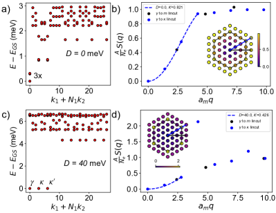
Figure 2: FCI-to-GWC transition driven by displacement field. (a, c) Many Body Spectra on a 27 site cluster at $\nu=2/3$, $\theta=2.8^{\circ}$, $\epsilon=10$ and $D=0,40$ meV respectively. There is a clear near 3-fold degeneracy at $\gamma$ for $D=0$ meV that moves to $\gamma$, $\kappa$, $\kappa^{\prime}$ for $D=40$ meV. (b, d) $\gamma$ to $\kappa$ and $\gamma$ to $M$ linecut of $S(\mathbf{q})$ with the corresponding parameters of (a, c). The 2d inset shows the full $S(\mathbf{q})$ one momentum shell outside of the Brillouin Zone and the points according to their corresponding linecuts.

Results—. We now study the phase diagram of $t$MoTe₂ as displacement field is turned on. Focusing first on $\nu=2/3$ where the FCI state is most robust, we present in Fig. 2 the many-body spectra (MBS) (the energy spectrum partitioned by momentum sector) and ground-state structure factor for $D=0$ and $D=40$ meV, where the lowest moiré band is separated from remote bands and has $C=1$ and $C=0$ respectively. Calculations were done at twist angle $\theta=2.8^{\circ}$ on a $N=27$ cluster with dielectric constant $\epsilon=10$.

For $D=0$, we find three nearly-degenerate ground states in the same momentum sector, consistent with the previously identified FCI phase on this cluster geometry [31]. In contrast, for $D=40$ meV, we find three degenerate ground states at distinct many-body momenta $\gamma,\kappa,\kappa^{\prime}$, which is consistent with a $\sqrt{3}\times\sqrt{3}$ GWC [43].

The emergence of GWC that spontaneously breaks lattice translation symmetry can be diagnosed by the structure factor. Indeed, for $D=40$ meV, $S(\mathbf{q})$ shows a prominent peak at the expected wavevector. Moreover, the peak height is found to increase with system size, which demonstrates the presence of long-range charge-density wave order, as shown in Fig. 3 (c-d). The existence of $\sqrt{3}\times\sqrt{3}$ GWC is expected at large $D$, when charges reside on the MX moiré sites on one layer and form a honeycomb superstructure with tripled unit cell to minimize the Coulomb repulsion, similar to the case of TMD heterobilayers [48]. In contrast, the structure factor of the FCI state at $D=0$ is liquid like and qualitatively similar to that of the $\nu=2/3$ fractional quantum Hall state in the lowest Landau level.

We further analyze the structure factor $S(\mathbf{q})$ at small $\mathbf{q}$ and extract the quantum weight $K$ by a quadratic fitting shown in Fig. 2 (b) and (d) (see Supplementary Material for details). We find $K=0.821$ at $D=0$, which indeed satisfies the universal topological bound of FCIs with $C=2/3$. In contrast, at $D=40$ meV, $K=0.426$ falls below $2/3$, which rules out the possibility of a $C=2/3$ FCI and instead is consistent with a topologically trivial state $C=0$. Our structure factor analysis shows that quantum weight can provide a useful method to distinguish topological and trivial states using a single ground state.

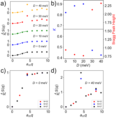
Figure 3: $S(\mathbf{q})$ and quantum weight at various displacement fields for $\nu=2/3$, $\theta=2.8^{\circ}$ and $\epsilon=10$. (a) $S(\mathbf{q})$ of the $\gamma$ to $\kappa$ linecut $S(\mathbf{q})$ vertically displaced to show dependence on displacement field. Bragg peaks emerge at $\kappa$ for $D=30,40$ meV and scale accordingly. (b) Quantum Weight and $S(\mathbf{q})$ value of $\kappa,\kappa^{\prime}$ Bragg peak vs Displacement field. (c, d) $S(\mathbf{q})$ at increasing commensurate system size at $D=0,40$ meV respectively. Bragg peaks emerge and scale as system size in the GWC phase as expected.

We extend this analysis further to identify the phase transition from FCI to GWC as the displacement field $D$ increases. Fig. 3 (a) shows $S(\mathbf{q})$ along the direction $\gamma-\kappa$ at increasing $D$. From $D=0$ to 20 meV, $S(\mathbf{q})$ as a function of $\mathbf{q}$ increases smoothly from 0 to 1, characteristic of a quantum liquid. At $D=30$ meV, a CDW Bragg peak arises abruptly and its magnitude increases further with $D$. Moreover, Fig. 3 (b) shows that immediately when the Bragg peak develops, the $K$ falls below 2/3. Our findings provide strong evidence for a direct transition between FCI and GWC, which appears to be first-order as evidenced by the discontinuity in quantum weight.

Experiments on $t$MoTe₂ have indeed observed at $\nu=2/3$ a transition from FCI to a trivial insulating state ($\sigma_{xy}=0$) under increasing displacement field [30]. The latter is consistent with the GWC, whose $\sqrt{3}\times\sqrt{3}$ charge order may be detected by scanning tunneling microscopy, or identified through different exciton energy shifts at inequivalent moiré sites in the tripled unit cell of the GWC.

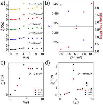
Figure 4: $S(\mathbf{q})$ and quantum weight at various displacement fields for $\nu=1/3$, $\theta=2.0^{\circ}$ and $\epsilon=10$. (a) $S(\mathbf{q})$ of the $\gamma$ to $\kappa$ linecut similar to Fig. 2. (b) Quantum Weight and $S(\mathbf{q})$ value of $\kappa,\kappa^{\prime}$ Bragg peak vs Displacement field. (c, d) $S(\mathbf{q})$ at increasing commensurate system size at $D=0,10$ meV respectively. Bragg peaks emerge and scale as system size in the GWC phase as expected.

We also study $t$MoTe₂ at $\nu=1/3$. Previous numerical studies at $D=0$ [31] have predicted that the $1/3$ state is a trivial $\sqrt{3}\times\sqrt{3}$ GWC at most of the twist angles, except in the neighborhood of a magic angle where the underlying Chern band is most lowest Landau level-like, giving rise to a $C=1/3$ FCI. In this case, our calculations find a similar FCI-to-GWC transition under increasing displacement field, as shown in Fig. 4. Compared to $\nu=2/3$, the FCI-to-GWC transition occurs at a smaller displacement field for $\nu=1/3$.

It is worth noting that across the $D$-induced transition from FCI to GWC at $\nu=2/3$ or $1/3$, the presence of Bragg peak in the structure factor at CDW wavevector is accompanied by a reduction of $S(\mathbf{q})$ at small $\mathbf{q}$, i.e., a decrease of quantum weight. This is not a coincidence and can be heuristically understood from energetic considerations as follows: the transition to the GWC is expected to lower the interaction energy, which is directly related to the structure factor: $E_{\rm int}=\sum_{\mathbf{q}}V(\mathbf{q})\left(\frac{A}{N_{e}}S(\mathbf{q})-1\right)/2A$, where Coulomb interaction $V(\mathbf{q})=2\pi e^{2}/\epsilon|\mathbf{q}|$ is positive at all $\mathbf{q}$, $N_{e}$ is the number of electrons in the system, and $A$ is the system area. On the other hand, the development of Bragg peak in the GWC, however, indicates that $S(\mathbf{q})$ increases at the CDW wavevector. Therefore, the reduction of interaction energy can only be possible due to the decrease of $S(\mathbf{q})$ at other wavevectors, including small $\mathbf{q}$. We confirm the reduction of $E_{int}$ across the FCI-to-GWC transition in the Supplementary Material.

Figure 5: Illustration of the universal topological bound being respected at fractional fillings. Extracted quantum weight is plotted versus twist angle at $\nu=1/3,2/3,1$ (orange, blue, black respectively). The universal topological bound for each filling is plotted as a solid horizontal line in the appropriate color, and the phase of the system at each angle is denoted by the style of the point. The diamonds correspond to points within the FCI phase; the solid circles correspond to points within the GWC phase; the hallow circles correspond to unconfirmed phases [31]. The dashed black line is the non-interacting case, previously shown to respect the topological bound in this system at integer filling [12]. All data is calculated at $\epsilon=10$ and $D=0$ on a 27 site cluster.

Finally, we calculate the structure factor and extract the quantum weight at $D=0$ as a function of twist angle for fillings $\nu=1/3$ and $2/3$ in Fig. 5. For $\nu=1/3$, the system transitions from an FCI to a GWC at $\theta\approx 2.3^{\circ}$, as indicated by the emergence of Bragg peaks, in agreement with the previous study [31]. We note in passing that unlike the GWC at large $D$, here the quantum weight of GWC at larger angle still exceeds $1/3$. Thus while the violation of topological bound suffices to rule out a (fractional) Chern insulator with many-body Chern number $C$, the converse is not true: a large quantum weight $K>|C|$ does not guarantee topological order.

It is interesting to note that the quantum weight of FCI states at $D=0$ reaches a minimum and nearly saturates the topological bound at a magic angle, which is around $1.75^{\circ}$ for $\nu=1/3$, and lies between $1.75^{\circ}$ and $2^{\circ}$ for $\nu=2/3$. This is broadly consistent with the theoretical picture that the moiré band wavefunction at the magic angle closely resembles the lowest Landau level [25, 35], and therefore the corresponding FCI states closely resembles the fractional quantum Hall states, whose quantum weight saturates the topological lower bound.

Perhaps more remarkable is that the $\nu=2/3$ FCI persists to larger angles where the quantum weight far exceeds the topological bound. At $\theta=3.75^{\circ}$, $K=1.034$ is almost twice the bound, signifying a considerably difference between the FCI and the fractional quantum Hall state. It will be interesting to construct variational wavefunction for such non-standard FCI states featuring large quantum weight.

Discussion—. In this work, we mapped out the phase diagram for $t$MoTe₂ at $\nu=1/3$ and $2/3$ as a function of displacement field based primarily on the structure factor calculated by band-projected ED. We use $S(\mathbf{q})$ to distinguish liquid and crystal states, and uncover a displacement field induced topological phase transition using the quantum weight $K$. Our numerical results confirm the topological bound $K\geq|C|$ found by Oinishi and Fu for FCIs and identify the magic angle where this bound is nearly saturated.

We note that band-projected ED is quantitatively accurate when the band gap is large compared to interaction energy. However, near the critical field where the band gap closes and band topology changes $C=1\rightarrow 0$, band mixing may affect the many-body ground states at fractional filling. Nonetheless, our band-projected ED provides variational ground state energies and wavefunctions, which serve as a useful starting point and benchmark for further investigation with advanced numerical methods.

Our work has shown that the static structure factor encodes a wealth of information about topological and correlated states in twisted TMDs. Measuring $S(\mathbf{q})$ directly with conventional x-ray scattering techniques is an experimental challenge due to the ultra-thin nature of 2D layers. In this regard, it is worth noting that the small-$q$ behavior of $S(\mathbf{q})$ encapsulated by the quantum weight can be directly determined from terahertz optical conductivity using the sum rule [5]:

$$K=2\hbar\int_{0}^{\infty}d\omega\frac{{\rm Re}\sigma_{xx}}{\omega},$$ (8)

where the frequency integration should encompasses the energy range of the continuum model for low-energy moiré bands.

Supplementary Material

I. Structure Factor Formalism

A. Explicit Calculation

The static structure factor is defined in the main text is the Fourier transform of the static density-density correlation function, $\tilde{S}(\bm{q})=\frac{1}{A}\langle\rho(\bm{q})\rho(\bm{-q})\rangle$ for general fermionic momentum-space density operators $\rho(\bm{q})=\sum_{\bm{k}}f^{\dagger}_{\bm{k}}f_{\bm{k}+\bm{q}}$ in the plane wave basis. Here in the supplement, we use the standard convention employed in exact diagonalization studies: $S(\bm{q})=\frac{A}{N_{e}}\tilde{S}(\bm{q})=\frac{1}{N_{e}}\langle\rho(\bm{q})\rho(\bm{-q})\rangle$ for number of electrons $N_{e}$ and system area $A$. This convention used in the supplement is to make $S(\bm{q})$ dimensionless, which eases notation of the calculations made in the supplement. The convention used in the main text is done to make quantum weight $K$ dimensionless, as it had been defined in previous works [5]. Referring to equation 7 in the main text, combining the definition of the fermionic momentum-space density operators in the continuum model with the definition of the structure factor, the explicit form of the static structure factor becomes

$$S(\bm{q})=\frac{1}{N_{e}}\left\langle\sum_{\sigma_{1},X_{1},\bm{k_{1}}}f^{\dagger}_{\sigma_{1},X_{1},\bm{k_{1}}}f_{\sigma_{1},X_{1},\bm{k_{1}}+\bm{q}}\sum_{\sigma_{2},X_{2},\bm{k_{2}}}f^{\dagger}_{\sigma_{2},X_{2},\bm{k_{2}}}f_{\sigma_{2},X_{2},\bm{k_{2}}-\bm{q}}\right\rangle\\ =\frac{1}{N_{e}}\sum_{\begin{subarray}{c}\sigma_{1},X_{1},\bm{k_{1}}\\ \sigma_{2},X_{2},\bm{k_{2}}\end{subarray}}\Bigg{\langle}\sum_{\begin{subarray}{c}n_{1},n_{2},n_{3},n_{4}\\ \bm{G},\bm{G^{\prime}},\bm{G^{\prime\prime}},\bm{G^{\prime\prime\prime}}\end{subarray}}u^{*}_{\sigma_{1},n_{1};\bm{G},X_{1}}(\bm{k_{1}})c^{\dagger}_{\sigma_{1},n_{1},\bm{k_{1}}}u_{\sigma_{1},n_{2};\bm{G^{\prime}},X_{1}}(\bm{k_{1}}+\bm{q})c_{\sigma_{1},n_{2},\bm{k_{1}}+\bm{q}}\\ \times u^{*}_{\sigma_{2},n_{3};\bm{G^{\prime\prime}},X_{2}}(\bm{k_{2}})c^{\dagger}_{\sigma_{2},n_{3},\bm{k_{2}}}u_{\sigma_{2},n_{4};\bm{G^{\prime\prime\prime}},X_{2}}(\bm{k_{2}}-\bm{q})c_{\sigma_{2},n_{4},\bm{k_{2}}-\bm{q}}\Bigg{\rangle}.$$ (S1)

Using standard manipulation of fermionic raising and lowering operator algebra and conservation of momentum, we arrive at the full expression for the structure factor:

$$S(\bm{q})=\frac{1}{N_{e}}\sum_{\begin{subarray}{c}\sigma_{1},\sigma_{2},X_{1},\\ X_{2},\bm{k_{1}},\bm{k_{2}}\end{subarray}}\sum_{\begin{subarray}{c}n_{1},n_{2},\\ n_{3},n_{4}\end{subarray}}\sum_{\begin{subarray}{c}\bm{G},\bm{G^{\prime}},\\ \bm{G^{\prime\prime}},\bm{G^{\prime\prime\prime}}\end{subarray}}\Bigg{[}\delta_{\sigma_{1},\sigma_{2}}\delta_{n_{2},n_{3}}\delta_{\bm{k_{2}},\bm{k_{1}}+\bm{q}}u^{*}_{\sigma_{1},n_{1};\bm{G},X_{1}}(\bm{k_{1}})u^{*}_{\sigma_{2},n_{3};\bm{G^{\prime\prime}},X_{2}}(\bm{k_{2}})\\ \times u_{\sigma_{2},n_{4};\bm{G^{\prime}},X_{2}}(\bm{k_{2}}-\bm{q})u_{\sigma_{1},n_{2};\bm{G^{\prime\prime\prime}},X_{1}}(\bm{k_{1}}+\bm{q})\left\langle c^{\dagger}_{\sigma_{1},n_{1},\bm{k_{1}}}c_{\sigma_{2},n_{4},\bm{k_{2}}-\bm{q}}\right\rangle\\ +u^{*}_{\sigma_{1},n_{1};\bm{G},X_{1}}(\bm{k_{1}})u^{*}_{\sigma_{2},n_{3};\bm{G^{\prime}},X_{2}}(\bm{k_{2}})u_{\sigma_{2},n_{4};\bm{G^{\prime\prime}},X_{2}}(\bm{k_{2}}-\bm{q})u_{\sigma_{1},n_{2};\bm{G^{\prime\prime\prime}},X_{1}}(\bm{k_{1}}+\bm{q})\\ \times\left\langle c^{\dagger}_{\sigma_{1},n_{1},\bm{k_{1}}}c^{\dagger}_{\sigma_{2},n_{3},\bm{k_{2}}}c_{\sigma_{2},n_{4},\bm{k_{2}}-\bm{q}}c_{\sigma_{1},n_{2},\bm{k_{1}}+\bm{q}}\right\rangle\Bigg{]},$$ (S2)

which simplifies to our final analytic expression:

$$S(\bm{q})=\frac{1}{N_{e}}\sum_{\begin{subarray}{c}\sigma_{1},X_{1},\\ X_{2},\bm{k_{1}}\end{subarray}}\sum_{\begin{subarray}{c}n_{1},n_{2},n_{3}\\ \bm{G},\bm{G^{\prime}},\bm{G^{\prime\prime}},\bm{G^{\prime\prime\prime}}\end{subarray}}\Bigg{[}u^{*}_{\sigma_{1},n_{1};\bm{G},X_{1}}(\bm{k_{1}})u^{*}_{\sigma_{1},n_{3};\bm{G^{\prime\prime}},X_{2}}(\bm{k_{1}}+\bm{q})u_{\sigma_{1},n_{2};\bm{G^{\prime}},X_{2}}(\bm{k_{1}})u_{\sigma_{1},n_{3};\bm{G^{\prime\prime\prime}},X_{1}}(\bm{k_{1}}+\bm{q})\\ \times\left\langle c^{\dagger}_{\sigma_{1},n_{1},\bm{k_{1}}}c_{\sigma_{1},n_{2},\bm{k_{1}}}\right\rangle\\ +\sum_{\sigma_{2},\bm{k_{2}},n_{4}}u^{*}_{\sigma_{1},n_{1};\bm{G},X_{1}}(\bm{k_{1}})u^{*}_{\sigma_{2},n_{3};\bm{G^{\prime\prime}},X_{2}}(\bm{k_{2}})u_{\sigma_{2},n_{4};\bm{G^{\prime}},X_{2}}(\bm{k_{2}}-\bm{q})u_{\sigma_{1},n_{2};\bm{G^{\prime\prime\prime}},X_{1}}(\bm{k_{1}}+\bm{q})\\ \times\left\langle c^{\dagger}_{\sigma_{1},n_{1},\bm{k_{1}}}c^{\dagger}_{\sigma_{2},n_{3},\bm{k_{2}}}c_{\sigma_{2},n_{4},\bm{k_{2}}-\bm{q}}c_{\sigma_{1},n_{2},\bm{k_{1}}+\bm{q}}\right\rangle\Bigg{]}.$$ (S3)

Going forward, the first term will be referred to as the single body component of the structure factor (Since it only contains the momentum of one particle), $S_{1}(\bm{q})$, and the second term will be referred to as the normal ordered two body component (where $\left\langle:\rho(\bm{q})\rho(\bm{-q}):\right\rangle\equiv\left\langle c^{\dagger}c^{\dagger}cc\right\rangle$ denotes normal ordering), $S_{2}(\bm{q})$, such that $S(\bm{q})=\frac{1}{N_{e}}\left[S_{1}(\bm{q})+S_{2}(\bm{q})\right]$.

B. Numerical Calculation

In practice, calculating the second-quantized fermionic operators for all bands is too computationally expensive, which makes using the explicit form of the full structure factor cumbersome in numerical calculations. Remarkably, we can calculate the full structure factor solely from the components of the projected structure factor. To see this, let us first represent the structure factor in position space and decompose it into our one and two body components (assuming identical atoms):

$$\begin{split}S(\bm{q})&=\frac{1}{N_{e}}\left\langle\sum_{i,j}e^{-i\bm{q}(\bm{r}_{i}-\bm{r}_{j})}\right\rangle\\ &=\frac{1}{N_{e}}\left\langle\sum_{i=j}e^{-i\bm{q}(\bm{r}_{i}-\bm{r}_{j})}+\sum_{i\neq j}e^{-i\bm{q}(\bm{r}_{i}-\bm{r}_{j})}\right\rangle\\ &=\frac{1}{N_{e}}\left[S_{1}(\bm{q})+S_{2}(\bm{q})\right]=1+\frac{1}{N_{e}}S_{2}(\bm{q}).\end{split}$$ (S4)

Now we show that assuming the many-body ground state lives in the projected space, $P|\Psi_{GS}\rangle=|\Psi_{GS}\rangle$ for projection operator $P$, then

$$\begin{split}\bar{S_{2}}(\bm{q})&=\frac{1}{N_{e}}\left\langle:\bar{\rho}(\bm{q})\bar{\rho}(\bm{-q}):\right\rangle\\ &=\frac{1}{N_{e}}\left\langle P\sum_{i\neq j}e^{-i\bm{q}\bm{r}_{i}}P^{2}\sum_{j\neq i}e^{-i\bm{q}\bm{r}_{j}}P\right\rangle\\ &=\frac{1}{N_{e}}\left\langle P\sum_{i\neq j}e^{-i\bm{q}(\bm{r}_{i}-\bm{r}_{j})}P^{3}\right\rangle\\ &=\frac{1}{N_{e}}\left\langle\sum_{i\neq j}e^{-i\bm{q}(\bm{r}_{i}-\bm{r}_{j})}\right\rangle=S_{2}(\bm{q}).\end{split}$$ (S5)

Finally, since the projected structure factor can also be factorized into one and two body components, $\bar{S}(\bm{q})=\frac{1}{N_{e}}\left[\bar{S_{1}}(\bm{q})+\bar{S_{2}}(\bm{q})\right]$, the full structure factor takes on the following form, exclusively in terms of the projected components:

$$S(\bm{q})=1+\frac{1}{N_{e}}\bar{S_{2}}(\bm{q})=1+\frac{1}{N_{e}}\left[\bar{S}(\bm{q})-\bar{S_{1}}(\bm{q})\right].$$ (S6)

The band projected structure factor is simply:

$$\bar{S}(\bm{\tilde{q}})=\frac{1}{N_{e}}\left\langle\bar{\rho}(\bm{\tilde{q}})\bar{\rho}(\bm{-\tilde{q}})\right\rangle_{\bm{GS}}$$ (S7)

where $\bar{\rho}(\bm{\tilde{q}})=\sum_{\bm{\tilde{k}}}\bar{f}^{\dagger}_{\bm{\tilde{k}}}\bar{f}_{\bm{\tilde{k}}+\bm{\tilde{q}}}$ is the band projected fermionic momentum-space density operators , $N_{e}$ is the number of electrons in the system, $\bm{\tilde{k}}$, $\bm{\tilde{q}}$ are vectors in the MBZ, and $\left\langle\right\rangle_{\bm{GS}}$ represents averaging over all degenerate ground states. Note that for the ordinary structure factor, we would be dealing with $\bm{k}=\bm{\tilde{k}}+\bm{g}$ and $\bm{q}=\bm{\tilde{q}}+\bm{g}$ for $\bm{k}$ and $\bm{q}$ in the Brillouin Zone (BZ) and $\bm{g}$ a reciprocal lattice vector. WLOG and to ease notation, we denote $\bm{k}$ and $\bm{q}$ as momentum vectors in the MBZ for the remainder of this section. Thus, we work out an explicit form for our band-projected structure factor:

$$\bar{S}(\bm{q})=\frac{1}{N_{e}}\left\langle\sum_{\sigma_{1},\bm{k_{1}}}\bar{f}^{\dagger}_{\sigma_{1},\bm{k_{1}}}\bar{f}_{\sigma_{1},\bm{k_{1}}+\bm{q}}\sum_{\sigma_{2},\bm{k_{2}}}\bar{f}^{\dagger}_{\sigma_{2},\bm{k_{2}}}\bar{f}_{\sigma_{2},\bm{k_{2}}-\bm{q}}\right\rangle_{\bm{GS}}\\ =\frac{1}{N_{e}}\sum_{\begin{subarray}{c}\sigma_{1},\bm{g},\bm{k_{1}}\\ n_{1},n_{2}\end{subarray}}\Bigg{[}|F(\bm{k_{1}},\bm{k_{1}},n_{1},n_{2},\sigma_{1},\bm{g}_{\bm{q}})|^{2}\left\langle c^{\dagger}_{\sigma_{1},n_{1},\bm{k_{1}}}c_{\sigma_{1},n_{2},\bm{k_{1}}}\right\rangle_{\bm{GS}}\\ +\sum_{\begin{subarray}{c}\sigma_{2},\bm{g^{\prime}},\bm{k_{2}},\\ n_{3},n_{4}\end{subarray}}F(\bm{k_{1}},\bm{k_{1}}+\bm{q},n_{1},n_{2},\sigma_{1},\bm{g}_{\bm{q}})F(\bm{k_{2}},\bm{k_{2}}-\bm{q},n_{3},n_{4},\sigma_{2},\bm{g^{\prime}}_{-\bm{q}})\left\langle c^{\dagger}_{\sigma_{1},n_{1},\bm{k_{1}}}c^{\dagger}_{\sigma_{2},n_{3},\bm{k_{2}}}c_{\sigma_{2},n_{4},\bm{k_{2}}-\bm{q}}c_{\sigma_{1},n_{2},\bm{k_{1}}+\bm{q}}\right\rangle_{\bm{GS}}\Bigg{]}\\ =\frac{1}{N_{e}}\left[\bar{S_{1}}(\bm{q})+\bar{S_{2}}(\bm{q})\right],$$ (S8)

where $\{n_{i}\}_{i=1,2,3,4}$ run over the projected bands, $\bm{g}_{\bm{q}}\equiv\bm{q}-[\bm{q}]$ is the reciprocal lattice component of an arbitrary momentum vector $\bm{q}$, and $F(\bm{k_{1}},\bm{k_{2}},n_{1},n_{2},\sigma,\bm{g})=\sum_{\bm{g^{\prime}},X}u_{\sigma,n_{1};\bm{(\bm{g^{\prime}}+\bm{g})},X}^{*}(\bm{k_{1}})u_{\sigma,n_{2};\bm{\bm{g^{\prime}},X}}(\bm{k_{2}})$ is the form factor coming from the normalization of single particle Bloch states labeled by moiré crystal momentum, band index and spin, $|\bm{k},n,\sigma\rangle=\sum_{\bm{g},X}u_{\sigma,n;\bm{g},X}(\bm{k})|\bm{k}+\bm{g},n,X,\sigma\rangle$. The operator $\left[\right]$ replaces an arbitrary momentum vector with its “mesh” equivalent $\bm{k}$, where each $\bm{k}$ is an unique representative of crystal momentum within the MBZ “mesh”. From this convention, it follows that any arbitrary momentum vector, $\bm{q}=[\bm{q}]+\bm{g}_{\bm{q}}$, can be uniquely represented on a computational grid. Thus, the explicit form for $S(\bm{q})$ is simply $1+\frac{1}{N_{e}}\bar{S}_{2}(\bm{q})$ where $\bar{S}_{2}(\bm{q})$ is the second term in equation S8.

In this section, we provide a brief overview for how the quantum weight can be extracted from the full structure factor. As mentioned in the main text, the quantum weight, $K$, is the leading order coefficient of the structure factor in materials with $U(1)$ symmetry:

$$\tilde{S}(\bm{q})=\frac{K_{\alpha\beta}}{2\pi}q_{\alpha}q_{\beta}+\cdots,$$ (S9)

where $\bm{A}$ is the uniform $U(1)$ vector potential [12, 5]. It can also be shown by through a quantum geometric formulation of the structure factor $\tilde{S}(\bm{q)}=\int_{BZ}\frac{d^{d}\bm{k}}{(2\pi)^{d}}\text{Tr}\left[P(\bm{k})\big{(}P(\bm{k})-P(\bm{k}+\bm{q}\big{)}\right]$ for projection oporator $P(\bm{k})$, that $K$ is simply the integral of the Fubini-Study metric of the occupied bands over the BZ:

$$K^{\mu\nu}\equiv 2\pi\int_{BZ}\frac{d^{d}\bm{k}}{(2\pi)^{d}}g^{\mu\nu}$$ (S10)

for occupied bands $\mu,\nu$. This formulation, however, becomes very difficult to calculate in the strongly coupled limit. As such, we can find $K$ for the interacting or fractional case by calculating $S(\bm{q})$, fitting the low $q$ behavior and extracting the quadratic coefficient. Since $S(\bm{q})$ is an even function, we only need to use even-powered expansion coefficients in our fit. Since $S(\bm{q}=0)=0$, the first point of is fully determined and we must include at least the next 2 points to avoid over-fitting. Since the next two points in the 27 site cluster along the $\gamma$ to $\kappa$ linecut are 1/4 and 3/4 of the way to $\kappa$ from $\gamma$ respectively, fitting the next two points with only 1 quadratic coefficient has high variance and does not truly capture the $q\rightarrow 0$ behavior. As a result, we fit the first 4 points ($\gamma$ to $\kappa$), using $q^{2}$ and $q^{4}$ coefficients and extract the $q^{2}$ coefficient as the quantum weight $K$ (up to a numerical factor of $\frac{4\pi A}{N_{e}}=2\sqrt{3}\pi\frac{a_{M}^{2}}{\nu}$) (Since Bragg peaks are also not reflective of $q\rightarrow 0$ behavior, we fit the first 3 points with 1 quadratic coefficient when Bragg peaks are present). In Fig S1, we show that this extraction of $K$ converges nicely in the non-interacting case where we can go to larger system sizes. Fig. S1 demonstrates the minimal finite size effects in the quantum weight extraction of the 27 site cluster. The 27 site cluster (pictured in the inset of Fig. 2 in main text) has a favorable geometry with a maximal point density in the $\gamma$ to $\kappa$ line-cut, which in effect limits the finite size impact on the extracted quantum weight. Indeed the extracted quantum weight for the 27 site cluster is closer to the convergent value of $K=1.069$ than the next 5 system sizes (up to $N=121$), demonstrating the robustness of the extracted quantum weight on the 27 site cluser.

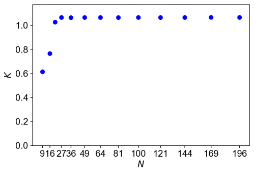
Figure S1: Extracted quantum weight as a function of system size for $\nu=1$ at $\theta=1.75^{\circ}$, $\epsilon=10$, and $D=0$.

III. Bragg Peak Scaling

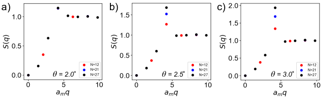
Figure S2: $S(\bm{q})$ vs $q$ along $\gamma$ to $\kappa$ linecut for $\nu=1/3$ at different system sizes. Panels (a-c) are demonstrated for $\theta=2.0^{\circ},2.5^{\circ},3.0^{\circ}$ respectively.

In order to evaluate how Bragg peaks scale with system size, we first note the expression for $S(\bm{q})$ with the Bragg peak divergence subtraced, otherwise known as the disconnected part of $S(\bm{q})$:

$$S(\bm{q})_{disconnected}=\frac{1}{N_{e}}\big{(}\langle\rho(\bm{q})\rho(\bm{-q})\rangle-\langle\rho(\bm{q})\rangle\langle\rho(\bm{-q})\rangle\big{)}$$ (S11)

The Bragg peaks themselves will scale as $S(\bm{q})-S(\bm{q})_{disconnected}=\frac{1}{N_{e}}\langle\rho(\bm{q})\rangle\langle\rho(\bm{-q})\rangle=\frac{1}{N_{e}}n(\bm{k})$, which is just the orbital occupation number divided by the particle number. Thus since the density operator scales on the order of system size, the Bragg peaks will also scale linearly with system size. In Fig. S2, $S(\bm{q})$ is plotted for $\nu=1/3$ at different system sizes for increasing $\theta$. As $\theta$ changes from $2^{\circ}$ to $3^{\circ}$, $t$MoTe₂ transitions from an FCI to a GWC, just like we show in the main text at $\theta=2.0^{\circ}$ as displacement field increases. While this transition at $\nu=1/3$ is already well known [31], we use the clear FCI to GWC transition to demonstrate the finite scaling signature of a crystal. With the current parameters, the system transitions from a FCI to a GWC at $\theta\approx 2.3^{\circ}$; however, the phases compete near this angle. From Fig. S2, peaks at $\kappa,\kappa^{\prime}$ clearly emerge as twist angle increases, and the Bragg peak scaling becomes conspicuously linear at $\theta=2.5^{\circ}$, conclusively demonstrating the Bragg peak signature of the electron crystal, as mentioned in the main text.

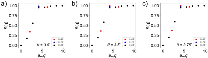
Figure S3: $S(\bm{q})$ vs $q$ along $\gamma$ to $\kappa$ linecut for $\nu=2/3$ at different system sizes. Panels (a-c) are demonstrated for $\theta=3.0^{\circ},3.5^{\circ},3.75^{\circ}$ respectively.

In sharp contrast, Fig. S3 shows that for $\theta>3.0^{\circ}$, where the system is outside the known FCI range, no clear crystal signature emerges. While Bragg peaks are present, they do not scale linearly with system size, indicating a non-pure crystalline state. These results add clarity to the potential phases beyond $\theta=3.0^{\circ}$ and reinforce the power fo the structure factor to help diagnosis phases of strongly correlated systems.

IV. Interaction Energy and Quantum Weight

As mentioned in the main text, we can relate the interaction energy, $\langle V\rangle_{GS}$, to the structure factor $S(\bm{q})$ since they both can be expressed in terms of fermionic momentum-space density operators. Specifically,

$$E_{int}=\langle\bm{V}\rangle=\left\langle\frac{1}{2}\sum_{\begin{subarray}{c}\sigma,\sigma^{\prime};\bm{k^{\prime}_{1}}\\ n_{1},n_{2},n_{3},n_{4};\\ \bm{k^{\prime}_{2}}\bm{k_{1}},\bm{k_{2}}\end{subarray}}V_{\bm{k^{\prime}_{1}}\bm{k^{\prime}_{2}}\bm{k_{1}}\bm{k_{2}}}^{\sigma\sigma^{\prime}}c^{\dagger}_{\sigma_{1},n_{1},\bm{k^{\prime}_{1}}}c^{\dagger}_{\sigma_{2},n_{3},\bm{k^{\prime}_{2}}}c_{\sigma_{2},n_{4},\bm{k_{2}}}c_{\sigma_{1},n_{2},\bm{k_{1}}}\right\rangle,$$ (S12)

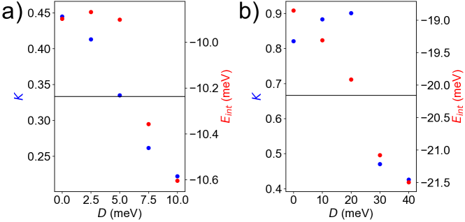
Figure S4: (a,b) Quantum weight and Interaction Energy as a function of displacement field for $\nu=1/3,2/3$ respectively. The drop in interaction energy is accompanied by drop in quantum weight, explaining why quantum weight experiences a sharp decrease in the GWC phase.

while Eq. S3 shows the similar form for $S(\bm{q})$. If we equate Eq. S12 with the second term in S3 (the normal ordered term) and sum over all $\bm{q}$, we arrive at the result:

$$E_{\rm int}=\sum_{\bm{q}}\frac{V(\bm{q})\left(S_{2}(\bm{q})/N_{e}\right)}{2A}=\sum_{\bm{q}}\frac{V(\bm{q})\left(S(\bm{q})-1\right)}{2A}$$ (S13)

where Coulomb interaction $V(\bm{q})=2\pi e^{2}/\epsilon|\bm{q}|$ is positive at all $\bm{q}$, $N_{e}$ is the number of electrons in the system, and $A$ is system area, as stated in the main text (The last equality follows from Eq. S6). In practice, we calculate $\bar{S}_{2}(\bm{q})$, which implies $E_{\rm int}=\sum_{\bm{q}}\frac{V(\bm{q})\left(\bar{S}_{2}(\bm{q})/N_{e}\right)}{2A}$ by Eq. S5. As noted in section I., the use of the band-projected structure factor is valid when the ground state wavefunction lives in the projected band subspace, which is indeed true for all systems studied in this paper. We noted that interaction energy decreases over the FCI-to-GWC transition since electrons localize to a configuration that minimizes energy. However the emergence of Bragg peaks indicates a spike of $S(\bm{q})$ at the reciprocal lattice harmonic wavevector. Thus, if interaction energy is lowered over this transition, $S(\bm{q})$ must decrease considerably for all other $\bm{q}$, namely for $\bm{q}\rightarrow 0$. We demonstrate this phenomena numerically in Fig. S4 by plotting the interaction energy and quantum weight side by side as the system undergoes the FCI-to-GWC transition under increasing displacement field.