LASER: Attention with Exponential Transformation

Abstract

Transformers have had tremendous impact for several sequence related tasks, largely due to their ability to retrieve from any part of the sequence via softmax based dot-product attention. This mechanism plays a crucial role in Transformer’s performance. We analyze the gradients backpropagated through the softmax operation in the attention mechanism and observe that these gradients can often be small. This poor gradient signal backpropagation can lead to inefficient learning of parameters preceeding the attention operations. To this end, we introduce a new attention mechanism called LASER, which we analytically show to admit a larger gradient signal. We show that LASER Attention can be implemented by making small modifications to existing attention implementations. We conduct experiments on autoregressive large language models (LLMs) with upto 2.2 billion parameters where we show upto 3.38% and an average of $\sim$1% improvement over standard attention on downstream evaluations. Using LASER gives the following relative improvements in generalization performance across a variety of tasks (vision, text and speech): 4.67% accuracy in Vision Transformer (ViT) on Imagenet, 2.25% error rate in Conformer on the Librispeech speech-to-text and 0.93% fraction of incorrect predictions in BERT with 2.2 billion parameters.

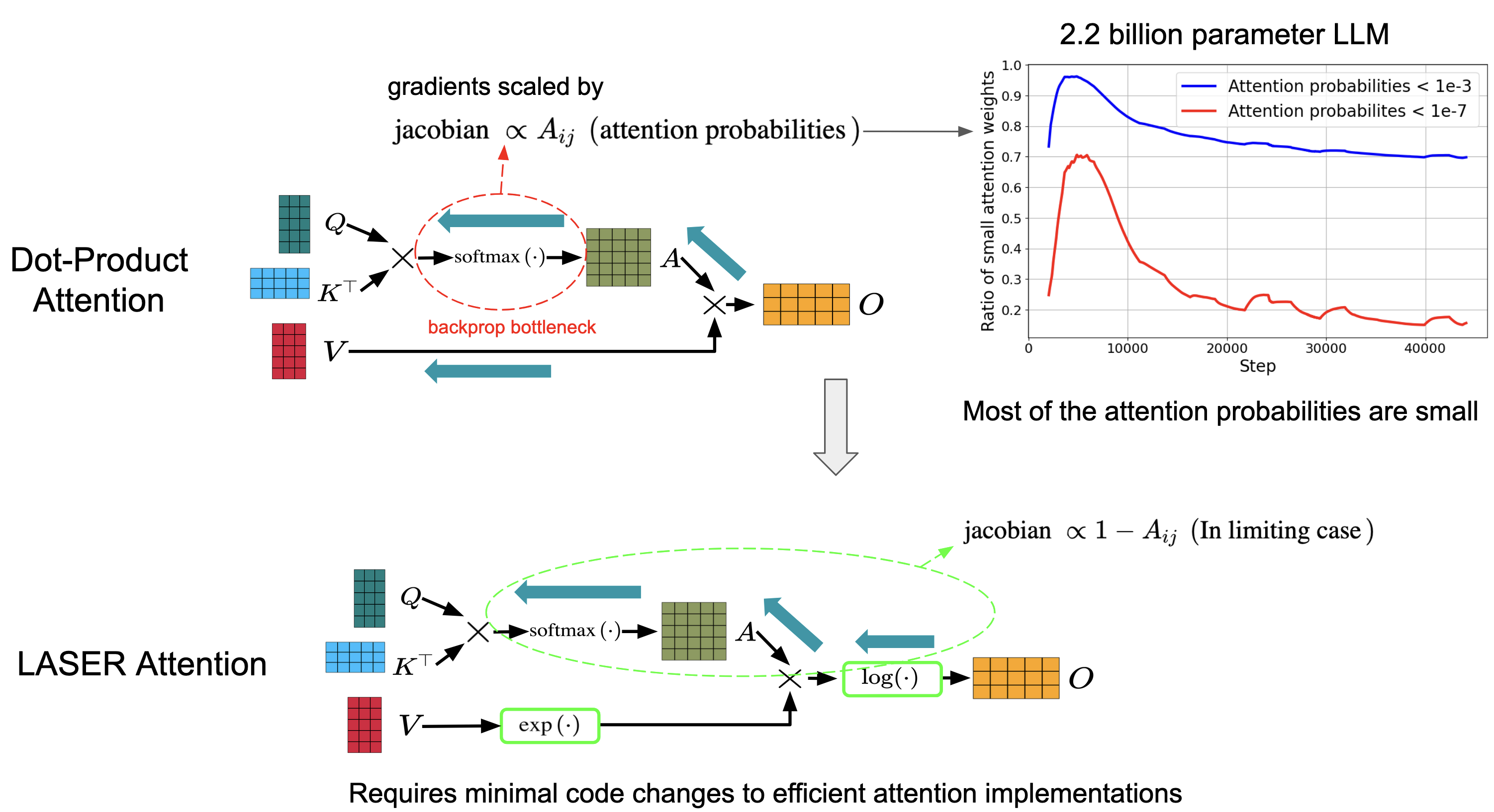
Figure 1: Backpropagating gradients through the softmax operation in the attention mechanism requires scaling with the Jacobian of softmax. We show that this Jacobian scales with attention probabilities/weights, which are typically small in large language models (LLMs) with about 80% of the probabilties less than $10^{-3}$ and about 20% less than $10^{-7}$. We propose LASER attention that involves conducting dot-product attention with an $\exp(\cdot)$-transformed value matrix $V$, i.e., conducting attention on $\exp(V)$. We show that LASER admits a larger Jacobian, is easier to implement and does not require any change to the underlying attention function, which may have a more nuanced implementation (e.g., FlashAttention (Dao et al., 2022)). In the image, $\exp(.)$ and $\log(.)$ are element-wise operations.

1 Introduction

Transformer architectures (Vaswani et al., 2017) have gained prominence over traditional models like LSTMs (Long-Short-Term-Memory) (Hochreiter & Schmidhuber, 1997) for various sequence-based tasks due to their ability to better capture long-range dependencies (Gemini, 2024; Meta-AI, 2024) without suffering from the vanishing gradient problem (Glorot & Bengio, 2010; Bengio et al., 1994). The attention mechanism plays a key role in Transformers, where different weights or probabilities are assigned to token representations in a sequence, indicating their relative importance, and these weights are computed via a softmax function (Vaswani et al., 2017). The Transformer architecture consists of multiple stacked layers comprising attention mechanism, where each layer operates on the output of the previous one, forming the Transformer encoder or decoder. Learning within a neural network is performed via gradient backpropagation, wherein gradients propagate backward through the network layer by layer using the chain rule (LeCun et al., 2002). During backpropagation, gradient magnitudes tend to diminish, resulting in a weaker gradient signal reaching the bottom layers and inefficient learning, which is called as vanishing gradient problem (Glorot & Bengio, 2010; Bengio et al., 1994). Residual connections (He et al., 2016) are used in Transformers so that gradients can bypass the layers via skip connections during backpropagation to improve the gradient magnitude for bottom layers, reinforcing the idea that architectures capable of efficient gradient backpropagation tend to offer better training performance.

In this paper, we theoretically analyze the gradient backpropagation in the attention mechanism of a Transformer and identify a vanishing gradient issue. During backpropagation, the gradient can be scaled by a very small value due to the softmax operation in the attention mechanism. Based on this observation, we propose a modification to the attention mechanism - LASER - LogArithm of Summed Exponentials of Representations. LASER is equivalent to conducting attention on exponentially transformed inputs and admits a log-sum-exp structure. We analytically show that gradients propagated via LASER attention are typically large. Since $\exp(\cdot)$ transformation in LASER can lead to numerical overflow, we develop a novel implementation - Log-Weighted-Sum-Exp trick, inspired from the Log-Sum-Exp trick (Blanchard et al., 2019). This technique allows LASER to scale to large models with upto 2.2 billion parameter models. We show that our implementation requires small modifications, and doesn’t need any changes to the underlying attention mechanism which might admit a more nuanced implementation, for e.g., FlashAttention (Dao et al., 2022).

We conduct thorough empirical verification across a variety of Transformer models: Conformer (Gulati et al., 2020) for Librispeech speech-to-text (Panayotov et al., 2015), Vision Transformer(Dosovitskiy et al., 2021) for ImageNet classification (Deng et al., 2009), decoder-only text Transformer (Brown et al., 2020) on C4 dataset (Raffel et al., 2020) and BERT ((Devlin et al., 2018)). We conduct experiments on decoder-only autoregressive language models from 234 million parameters to 2.2 billion parameter models, where we demonstate improvements of up to 1.7% relative improvement in test loss over standard attention. We conduct one-shot evaluation on 17 downstream tasks and show that LASER outperforms standard attention on 14 tasks with upto 3.38% improvement in accuracy and 1% accuracy improvement on average. On a 2.2 billion parameter BERT (Devlin et al., 2018), LASER gives a relative improvement of 0.93% on masked language modeling prediction error rate. LASER also demonstrates a 4.67% relative improvement in validation error rate in Vision Transformer and 1.2% absolute improvement in accuracy, and a 2.25% relative improvement in validation word error rate in the Conformer benchmark.

2 Related Work

The attention mechanism was used in Bahdanau et al. (2015) to drastically improve machine translation performance compared to encoder-decoder recurrent neural networks (RNNs) (Cho, 2014). This was later adopted in Transformers (Vaswani et al., 2017), which introduced self-attention to improve the performance in machine translation even further. Efficient attention mechanisms have been an active area of research due to the quadratic computational complexity in sequence length of Attention, which prevents long-context language modeling. One notable contribution is Linear Attention (Katharopoulos et al., 2020), which reduces the quadratic complexity of self-attention to linear in sequence length by using kernel approximation of the softmax operation. Similarly, the Performer (Choromanski et al., 2021) develops an alternative kernel approximation using random feature maps to achieve linear complexity.

The Mamba architecture introduces state-space models (SSMs) as a replacement for traditional attention. Models like S6 (S4+selection+scan) (Gu & Dao, 2023) from Mamba and SSD from Mamba-2 (Dao & Gu, 2024) have linear computational complexity in sequence length without the use of attention. However, despite these innovations, attention-based models like Gemini 1.5 Flash (Gemini, 2024) and LLaMA 3 (Dubey et al., 2024) continue to dominate long context regime, particularly through advancements in context parallelism (Liu et al., 2023), which ensures scalability while maintaining the strengths of attention mechanisms in Transformer models.

Efficient attention mechanisms have become critical in handling long sequences, especially in Transformer-based architectures. This mechanism is used for faster inference and training, particularly when scaling up to large sequence lengths. Sparse Transformers (Child et al., 2019) use fixed sparse attention patterns, enabling them to efficiently handle very long sequences by reducing the quadratic complexity of standard attention to linear or sub-quadratic in practice. Routing Transformers (Roy et al., 2021) take a different approach by introducing a mechanism that sparsifies attention through data-dependent sparsity patterns with subquadratic computational complexity in sequence length. Similarly, Longformer (Beltagy et al., 2020) modifies the standard self-attention mechanism to handle long documents by combining local windowed attention with global attention. FlashAttention (Dao et al., 2022; 2024) is a recent advancement that reduces HBM memory accesses by using GPU SRAM during attention computation, improving the speed of attention computation. LASER Attention can be thought of as complementing these approaches, as it conducts attention using the exponential transformation of inputs, without any change to the underlying attention function.

3 LASER Attention: LogArithm of Summed Exponentials of Representations

We first formally introduce Transformers (Vaswani et al., 2017) and the underlying softmax dot-product attention in Section 3.1. In Section 3.2, we introduce LASER Attention by first deriving the gradients of standard attention by making observations on a simple case of sequence length $2$, and then generalizing to larger sequence lengths.

3.1 Transformers and Softmax Dot-Product Attention

Let $X\in\mathbb{R}^{N\times d}$ represent the input sequence with $N$ tokens, where the $i$-th row is a $d$-dimensional representation of the $i$-th token. We describe the Transformer layer $T:\mathbb{R}^{N\times d}\to\mathbb{R}^{N\times d}$ similar to Katharopoulos et al. (2020) as follows:

$$T(X)=f(X+\operatorname{attn}(X)W_{O}),$$ (1)

where $f:\mathbb{R}^{N\times d}\to\mathbb{R}^{N\times d}$ is usually implemented using a 2-layer feed-forward neural network which acts on each token representation independently and $W_{O}\in\mathbb{R}^{d\times d}$ is a tunable parameter matrix. The attention function $\operatorname{attn}(.)$ is the only operation in the Transformer which is applied across the sequence axis. A single headed attention mechanism (Vaswani et al., 2017) can be described as follows:

$$Q=XW_{Q},\quad K=XW_{K},\quad V=XW_{V},$$

$$\tilde{A} =QK^{\top}$$

$$\operatorname{attn}(X) =\operatorname{softmax}(\tilde{A})V,$$ (2)

where $Q,K,V,\operatorname{attn}(X)\in\mathbb{R}^{N\times d}$. The $\operatorname{softmax}$ (Bridle, 1990) operation is applied for each row $\tilde{a}$ of attention logits $\tilde{A}=QK^{\top}$ separately:

$$(\operatorname{softmax}(\tilde{a}))_{i} =\exp(\tilde{a}_{i})/\left(\sum_{j=1}^{N}\exp(\tilde{a}_{j})\right).$$

Layer normalizations (Ba et al., 2016) are usually applied before or after $f(.)$ and $\operatorname{attn}(.)$ (Xiong et al., 2020), but we omit this for brevity. A Transformer is a composition of multiple layers (1) — $T_{l}(X)$, $\l\in\{1,\ldots,L\}$ sandwiched by the input embedding layer $E:\mathbb{R}^{N\times V}\to\mathbb{R}^{N\times d}$ and output softmax layer $S:\mathbb{R}^{N\times d}\to\mathbb{R}^{N\times V}$ as follows:

$$\operatorname{Transformer}(Z)=S\circ T_{L}\circ\cdots\circ T_{1}\circ E\ (Z)\in\mathbb{R}^{N\times V},$$

where the inputs to the network $Z\in\mathbb{R}^{N\times V}$. Thus choosing a suboptimal attention function $\operatorname{attn}(.)$ can affect every layer of the final $\operatorname{Transformer}(.)$. Let $\ell(\operatorname{Transformer}(Z),Y)$ be the loss function used to learn the parameters of the Transformer, where $Y$ is the true label information. Autoregressive language modeling (Radford et al., 2018; Brown et al., 2020) involves using a causal mask $M$, which is a lower triangular matrix, and is multiplied before the softmax operation as follows:

$$\operatorname{attn}(X) =\operatorname{softmax}(M\odot QK^{\top})V,$$

$$M_{ij} =\mathbbm{1}\{i\leq j\}$$

where $\odot$ denotes element-wise multiplication. During training, the gradients $\frac{\partial\ell}{\partial W_{K}},\ \frac{\partial\ell}{\partial W_{Q}},\ \frac{\partial\ell}{\partial W_{V}}$ are computed via backpropagation in a layer-by-layer fashion from layer $L$ to layer $1$ and are used to update the parameters. In the next section, we analyze the gradient backpropagation through $\operatorname{attn}(.)$ and propose LASER attention.

3.2 Gradient Analysis of Attention

For simplicity, we first let the sequence length $N$ be $2$ with attention probabilities $A=\operatorname{softmax}(KQ^{\top})$ and attention logits as $\tilde{A}=KQ^{\top}$. Expanding the matrices $A$ and $\tilde{A}$, we get:

$$A=\begin{pmatrix}a_{11}&a_{12}\\ a_{21}&a_{22}\end{pmatrix} =\operatorname{softmax}\begin{pmatrix}\tilde{a}_{11}&\tilde{a}_{12}\\ \tilde{a}_{21}&\tilde{a}_{22}\end{pmatrix}$$

$$=\begin{pmatrix}\frac{\exp(\tilde{a}_{11})}{\exp(\tilde{a}_{11})+\exp(\tilde{a}_{12})}&\frac{\exp(\tilde{a}_{12})}{\exp(\tilde{a}_{11})+\exp(\tilde{a}_{12})}\\ \frac{\exp(\tilde{a}_{21})}{\exp(\tilde{a}_{21})+\exp(\tilde{a}_{22})}&\frac{\exp(\tilde{a}_{22})}{\exp(\tilde{a}_{21})+\exp(\tilde{a}_{22})}\end{pmatrix}$$

Dividing the numerators and denominators by $\exp(\tilde{a}_{ij})$ gives:

$$A=\begin{pmatrix}a_{11}&a_{12}\\ a_{21}&a_{22}\end{pmatrix} =\begin{pmatrix}\frac{1}{1+\exp(\tilde{a}_{12}-\tilde{a}_{11})}&\frac{1}{\exp(\tilde{a}_{11}-\tilde{a}_{12})+1}\\ \frac{1}{1+\exp(\tilde{a}_{22}-\tilde{a}_{21})}&\frac{1}{\exp(\tilde{a}_{21}-\tilde{a}_{22})+1}\end{pmatrix}$$

$$=\begin{pmatrix}\sigma(\tilde{a}_{11}-\tilde{a}_{12})&1-\sigma(\tilde{a}_{11}-\tilde{a}_{12})\\ \sigma(\tilde{a}_{21}-\tilde{a}_{22})&1-\sigma(\tilde{a}_{21}-\tilde{a}_{22})\end{pmatrix},$$ (3)

where $\sigma$ denotes the sigmoid operation $\sigma(x)=1/(1+\exp(-x))$. As in (2), we now multiply the attention probabilities $A$ with the value matrix $V$. For simplicity, let the representation dimension $d=1$, then the attention output will be as follows:

$$\text{Attention output:}\ \ \operatorname{attn}(X)=\begin{pmatrix}o_{1}\\ o_{2}\end{pmatrix} =AV=\begin{pmatrix}\sigma(\tilde{a}_{11}-\tilde{a}_{12})v_{1}+(1-\sigma(\tilde{a}_{11}-\tilde{a}_{12}))v_{2}\\ \sigma(\tilde{a}_{21}-\tilde{a}_{22})v_{1}+(1-\sigma(\tilde{a}_{21}-\tilde{a}_{22}))v_{2}\end{pmatrix},$$ (4)

where $V=\begin{pmatrix}v_{1}\\ v_{2}\end{pmatrix}$. We now find the gradient with respect to $\tilde{A}$ via the chain rule:

$$\underbrace{\frac{\partial\ell}{\partial\tilde{A}}}_{\text{backpropagated gradient}}=\frac{\partial\ell}{\partial\operatorname{attn}(X)}\cdot\underbrace{\frac{\partial\operatorname{attn}(X)}{\partial\tilde{A}}}_{\text{Jacobian}}.$$

Thus, small Jacobian magnitude can lead to small backpropagated gradient. We now analyze an element of the Jacobian:

$$\operatorname{attn}\text{ Jacobian:}\ \ \frac{\partial o_{1}}{\partial\tilde{a}_{11}} =v_{1}\sigma(\tilde{a}_{11}-\tilde{a}_{12})(1-\sigma(\tilde{a}_{11}-\tilde{a}_{12}))-v_{2}\sigma(\tilde{a}_{11}-\tilde{a}_{12})(1-\sigma(\tilde{a}_{11}-\tilde{a}_{12}))$$

$$=(v_{1}-v_{2})\underbrace{\sigma(\tilde{a}_{11}-\tilde{a}_{12})(1-\sigma(\tilde{a}_{11}-\tilde{a}_{12}))}_{\text{possible saturation}}.$$ (5)

The sigmoid function value, $\sigma(\tilde{a}_{11}-\tilde{a}_{12})$ saturates to $1$ when $\tilde{a}_{11}-\tilde{a}_{12}$ becomes sufficiently large. Conversely, when $\tilde{a}_{11}-\tilde{a}_{12}$ is large and negative, the function value saturates to $0$. In both cases, saturation leads to vanishing gradients, where the gradient becomes very small. This phenomenon is a well-documented limitation of the sigmoid function (LeCun et al., 2002).

We extend this observation to sequence length of size $N$ as follows:

Lemma 3.1 (Gradient saturation in softmax).

Let $a\in\mathbb{R}^{N}$ be a row in attention weights/probabilities $A$ and similarly let $\tilde{a}$ be a row in attention logits $\tilde{A}$, then:

forward pass: $$\quad a=\operatorname{softmax}(\tilde{a}),$$

backward pass: $$\quad\frac{\partial\ell}{\partial\tilde{a}}=(\operatorname{diag}(a)-aa^{\top})\frac{\partial\ell}{\partial a},$$

softmax Jacobian: $$\quad\frac{\partial a_{j}}{\partial\tilde{a}_{i}}=a_{j}(\mathbbm{1}\{i=j\}-a_{i}),$$

where $\operatorname{diag}(a)$ denotes the diagonal matrix with diagonal elements $a$.

We give a proof of this lemma in Section A.2

To address this issue, we now introduce LASER Attention which applies attention in exponential value space, $\exp(V)$, as follows:

$$\exp(\operatorname{laser}(X)) =\operatorname{softmax}(QK^{\top})\exp(V)$$

$$\implies\operatorname{laser}(X) =\log(\operatorname{softmax}(QK^{\top})\exp(V))\quad\rightarrow\quad\text{LASER Attention},$$ (6)

where $\log(.)$ and $\exp(.)$ are applied elementwise. Expanding (6) for $N=2$ and $d=1$ as done for standard attention (4) gives:

$$\text{LASER output: }\begin{pmatrix}o_{1}\\ o_{2}\end{pmatrix}=\begin{pmatrix}\log(\sigma(\tilde{a}_{11}-\tilde{a}_{12})\exp(v_{1})+(1-\sigma(\tilde{a}_{11}-\tilde{a}_{12}))\exp(v_{2}))\\ \log(\sigma(\tilde{a}_{21}-\tilde{a}_{22})\exp(v_{1})+(1-\sigma(\tilde{a}_{21}-\tilde{a}_{22}))\exp(v_{2}))\end{pmatrix},$$ (7)

Low gradient saturation. Computing an element in the Jacobian ${\partial\operatorname{laser}(X)}/{\partial\tilde{A}}$ as done for standard attention in (5) gives the following:

$$\text{LASER Jacobian:}\quad\frac{\partial o_{1}}{\partial\tilde{a}_{11}} =\frac{(\exp(v_{1})-\exp(v_{2}))\sigma(\tilde{a}_{11}-\tilde{a}_{12})(1-\sigma(\tilde{a}_{11}-\tilde{a}_{12}))}{\sigma(\tilde{a}_{11}-\tilde{a}_{12})\exp(v_{1})+(1-\sigma(\tilde{a}_{11}-\tilde{a}_{12}))\exp(v_{2})}$$

$$=\frac{(\exp(v_{1})-\exp(v_{2}))\sigma(\tilde{a}_{11}-\tilde{a}_{12})(1-\sigma(\tilde{a}_{11}-\tilde{a}_{12}))}{\sigma(\tilde{a}_{11}-\tilde{a}_{12})(\exp(v_{1})-\exp(v_{2}))+\exp(v_{2})}.$$

We now consider a limiting case to simplify the above equation: if $v_{1}-v_{2}\gg 0$, then

$$\text{LASER Jacobian:}\quad\frac{\partial o_{1}}{\partial\tilde{a}_{11}} =\frac{\sigma(\tilde{a}_{11}-\tilde{a}_{12})(1-\sigma(\tilde{a}_{11}-\tilde{a}_{12}))}{\sigma(\tilde{a}_{11}-\tilde{a}_{12})+\exp(v_{2})/(\exp(v_{1})-\exp(v_{2}))}$$

$$\approx\underbrace{(1-\sigma(\tilde{a}_{11}-\tilde{a}_{12}))}_{\text{low saturation}},$$

where the approximation is due to $\exp(v_{2})/(\exp(v_{1})-\exp(v_{2})\approx 0$.

Relation between LASER Attention and max function.

From definitions (3) and (7), LASER output can be written in a log-sum-exp form (Blanchard et al., 2019) as follows:

$$o_{1} =\log(a_{11}\exp(v_{1})+a_{12}\exp(v_{2}))$$

$$=\log(\exp(v_{1}+\log(a_{11})+\exp(v_{2}+\log(a_{12}))$$ (8)

Log-exp-sum function can be thought of as a differentiable approximation of $\max$ function:

Lemma 3.2 (Boyd & Vandenberghe (2004)).

The function $f(x_{1},\ldots,x_{n})=\log\left(e^{x_{1}}+\cdots+e^{x_{n}}\right)$ is convex on $\mathbb{R}^{n}$. This function can be interpreted as a differentiable approximation of the $\max$ function, since

$$\max\{x_{1},\dots,x_{n}\}\leq f(x_{1},\ldots,x_{n})\leq\max\{x_{1},\dots,x_{n}\}+\log n$$

for all $x\in\mathbb{R}^{n}$. (The second inequality is tight when all components of $x$ are equal.)

Given that $\max(x_{1},\ldots,x_{n})$ function is not differentiable at points where two or more elements take the same value, log-sum-exp can serve as a differentiable approximation. Using Lemma 3.2, we can relate LASER (8) to $\max(\cdot)$ operation as follows:

$$\max(v_{1}+\log(a_{11}),v_{2}+\log(a_{12}))\leq o_{1}\leq\max(v_{1}+\log(a_{11}),v_{2}+\log(a_{12}))+\log(2)$$

3.3 LASER Implementation via Log-Weighted-Sum-Exp Trick

In this section we explore implementing LASER and provide pseudocode. Given the log-sum-exp structure from (8):

$$o_{1}=\log(\sigma(\tilde{a}_{11}-\tilde{a}_{12})\exp(v_{1})+(1-\sigma(\tilde{a}_{11}-\tilde{a}_{12}))\exp(v_{2})),$$

one can notice that $\exp(.)$ operations can lead to overflow. This problem has been recognized in Blanchard et al. (2019) and the “log-sum-exp trick” is used to avoid overflows. However, the log-sum-exp trick cannot be applied directly as it would be difficult to implement without changing the underlying attention function. We propose a “log-weighted-sum trick”, where we subtract the maximum value $m=\max(v_{1},v_{2})$ from $v_{1}$ and $v_{2}$ and rewrite the above equation as follows:

$$o_{1} =\log((\sigma(\tilde{a}_{11}-\tilde{a}_{12})\exp(v_{1}-m)+(1-\sigma(\tilde{a}_{11}-\tilde{a}_{12}))\exp(v_{2}-m))*\exp(m))$$

$$=\log(\sigma(\tilde{a}_{11}-\tilde{a}_{12})\exp(v_{1}-m)+(1-\sigma(\tilde{a}_{11}-\tilde{a}_{12}))\exp(v_{2}-m))+m.$$

Now conducting $\exp(.)$ operation on $v_{1}-m$ and $v_{2}-m$ will not lead to overflows. We can extend this to matrix-version (6) by conducting column-wise maximum of value matrix $V\in\mathbb{R}^{N\times d}$ as follows:

$$m_{j} =\max_{i\in\{1,\ldots,N\}}V_{ij},\ j\in\{1,\ldots,d\}$$

Define $$\hat{V}\in\mathbb{R}^{N\times d}\text{ such that }\hat{V}_{ij}=(V_{ij}-m_{j}).$$

The above operations helps us conduct $\exp(.)$ operation without overflows. Then the final LASER attention operation would be as follows:

$$\text{Define $O\in\mathbb{R}^{N\times d}$ as: }O =\log(\operatorname{softmax}(QK^{\top})\exp(\hat{V})\operatorname{diag}(\exp(m)))$$

$$O_{ij} =(\log(\operatorname{softmax}(QK^{\top})\exp(\hat{V})))_{ij}+m_{j}.$$ (9)

Here, $m=(m_{1},\ldots,m_{d})$ and $\operatorname{diag}(m)$ is a diagonal matrix with elements of $m$ as diagonals. Log-weighted-sum-exp trick allows us to implement LASER attention via merely modifying the inputs and outputs of standard attention, without changing the underlying attention function. Additionally, we show in Section 4.1 that this trick helps avoid overflows in large scale settings. The following JAX (Bradbury et al., 2018) code demonstrates that LASER attention can be implemented by utilizing standard attention functions.

Algorithm 1 LASER Attention with Log-Weighted-Sum-Exp Trick

1:  Input: Values $V\in\mathbb{R}^{N\times d}$, Queries $Q\in\mathbb{R}^{N\times d}$, Keys $K\in\mathbb{R}^{N\times d}$

2:  Output: LASER Attention output $O\in\mathbb{R}^{N\times d}$

3:  Compute the column-wise maximum for the value matrix $V$:

$$m_{j} =\max_{i\in\{1,\ldots,N\}}V_{ij},\quad j\in\{1,\ldots,d\}$$

4:  Subtract $m_{j}$ from the $j$th column of $V$:

$$\hat{V}\in\mathbb{R}^{N\times d}\text{ such that }\hat{V}_{ij}=(V_{ij}-m_{j})\quad\text{// Shift values to avoid overflow in the following }\exp(.)$$

5:  Apply attention with Queries $Q$, Keys $K$ and Values $V$ with $m_{j}$, $j\in\{1,\ldots,d\}$ added back to the output, following (9)

$$\text{Define $O\in\mathbb{R}^{N\times d}$ as: }(O)_{ij}=(\log(\operatorname{softmax}(QK^{\top})\exp(\hat{V})))_{ij}+m_{j}$$

6:  return  LASER attention output $O$

4 Experimental Results

4.1 Autoregressive Language Modeling on C4

In this section, we compare the performance of LASER Attention with standard attention mechanisms in the context of an autoregressive language modeling task.

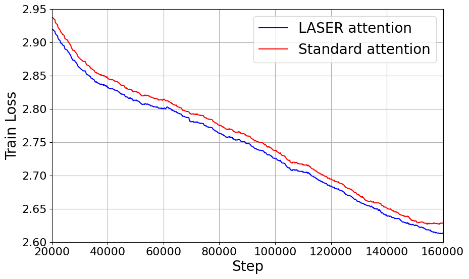
(a) Training Loss Comparison

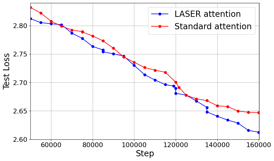
(b) Test Loss Comparison

Figure 2: Comparison between pretraining performance of LASER and standard attention mechanism on a 301 million parameter autoregressive language model with 32 layers, 2048 hidden dimension and 1024 model dimension on 168 billion tokens in C4 dataset. LASER attention shows consistently lower train (left) and test (right) loss values.

Dataset and Setup.

We use the C4 dataset (Raffel et al., 2020) for our experiments. The training is conducted using a batch size of 1024 sequences, each sequence has 1024 tokens. The models are trained for 160,000 iterations, resulting in the utilization of approximately 167.8 billion tokens. Throughout the training process, we monitor both the training and test losses, and we observe a significant improvement in the test set performance when using LASER Attention compared to the standard attention mechanism (as illustrated in Figure 2). We use the AdamW optimizer (Loshchilov & Hutter, 2017) paired with cosine learning rate schedule (Loshchilov & Hutter, 2016) with linear learning rate warmup followed by decay to zero at the end of the training.

Model Architecture.

The base model architecture consists of 301 million parameters of a decoder-only Transformer, which is distributed across 32 layers as defined in (1). Each layer uses 8 attention heads, with each head having a size of 128. The MLP block in this architecture, as defined in (1), has a hidden dimension of 2048.

In addition to this configuration, we also experiment with a variant where the model retains 32 layers but increases the MLP block hidden dimension to 4096. In this variant, we increase the hidden dimension of the MLP block to shift more parameters into the MLP block. This configuration continues to show improvements in both the training and test loss metrics, demonstrating that the effectiveness of LASER Attention is maintained even when attention parameters are reduced. The results of these experiments can be seen in Table 1, where we also include ablation results showing improvements even with a 16-layer setting.

Number of Layers	Hidden Dimension	LASER	Standard Attention
16	4096	2.673	2.681
32	2048	2.595	2.641
32	4096	2.555	2.575

Table 1: Comparison of test loss between LASER and Standard attention mechanisms across different distribution of parameters between MLP block $f(.)$ and attention $\operatorname{attn}(.)$ in (1), where we notice upto 1.74% relative improvement in loss.

Ablation with optimizers.

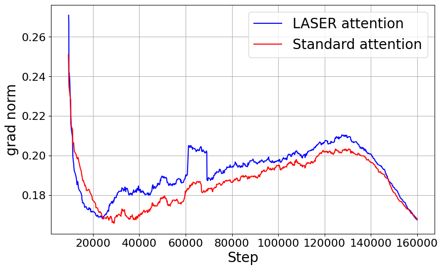
Figure 3: In this figure, we measure grad_norm vs steps for an autoregressive language model with a 301 million parameters model corresponding to Figure 2.

For the 301 million parameter model, we noticed in Figure 3 that LASER had higher gradient norm throughout training. An initial hypothesis was that higher gradient norms might lead to more parameter change, consequently reducing the loss more effectively. To investigate this, we utilized the LAMB optimizer (You et al., 2019), which normalizes and renormalizes updates using the weight norm to ensure that the scale of updates matches the scale of the weights, thus voiding the effect of gradient/update norms on optimization. Interestingly, even with LAMB’s normalization mechanism, we observed a consistent improvement in training (Standard Attention: 2.749 vs LASER: 2.736) and test loss (Standard Attention: 2.758 vs LASER: 2.741), suggesting that the performance gains were not solely driven by larger gradient magnitudes but are intrinsic to the model’s architecture and the LASER Attention mechanism.

Scaling to larger models.

To demonstrate the scalability of our approach, we conducted experiments on a 1.1 billion and 2.2 billion parameter model. We note that without using the log-weighted-sum-exp trick introduced in Section 3.3, the 2.2 billion parameter model training fails due to numerical overflow. In Figure 4, we show that LASER attention outperforms standard-attention in a 2.2 billion parameter model with model dimension 2048 and hidden dimension 8192 with 32 layers and 8 attention heads (each of size 512). We observe the same in 1.1 billion model (Figure 4), which has a scaled down hidden dimension (4096) and attention head size (256).

Evaluation on downstream tasks.

In Figure 2, we mention the performance of our 2.2 billion parameter model on several downstream tasks. Where we evaluate on ARC (Clark et al., 2018), BoolQ (Clark et al., 2019), CB (Wang et al., 2019), COPA (Wang et al., 2019), HellaSwag (Zellers et al., 2019), MultiRC (Khashabi et al., 2018), OpenBookQA (Mihaylov et al., 2018), PIQA (Bisk et al., 2020), RACE (Lai et al., 2017), ReCoRD (Zhang et al., 2018), RTE (Wang et al., 2019), StoryCloze (Mostafazadeh et al., 2016), WiC (Pilehvar & Camacho-Collados, 2019), Winograd (Levesque et al., 2012), Winogrande (Kocijan et al., 2020), and WSC (Wang et al., 2019). We found that LASER outperforms in 14 out 17 datasets with upto 3.38% difference and 0.85% difference on average in accuracy.

	WSC	Winogrande	Winograd	WiC	StoryCloze	RTE	ReCoRD
LASER	81.40	61.88	81.68	51.41	77.87	53.07	85.39
Standard	79.65	62.27	80.22	50.94	76.59	53.07	85.14

	RaceM	RaceH	PIQA	OpenBookQA	MultiRC	HellaSwag	COPA
LASER	50.56	37.71	77.26	48.80	57.51	66.56	82.00
Standard	49.44	37.65	76.88	47.60	54.13	65.49	80.00

	CB	BoolQ	ARC_Easy
LASER	41.07	63.52	61.53
Standard	44.64	60.58	60.82

Table 2: Accuracies of one-shot evaluation of 2.2 billion parameter autoregressive language model trained via LASER and standard attention. We found that LASER outperforms standard attention on 14 out of 17 datasets by upto 3.38%. On average LASER gives an accuracy of 63.48% vs standard attention (62.65%).

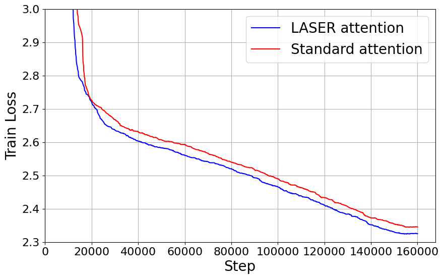
(a) Train loss - 2.2 billion parameter model.

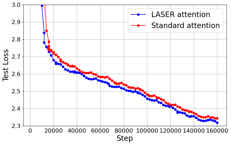
(b) Test loss - 2.2 billion parameter model.

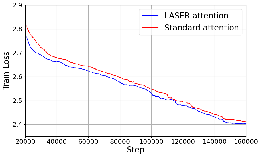
(c) Train loss - 1.1 billion parameter model.

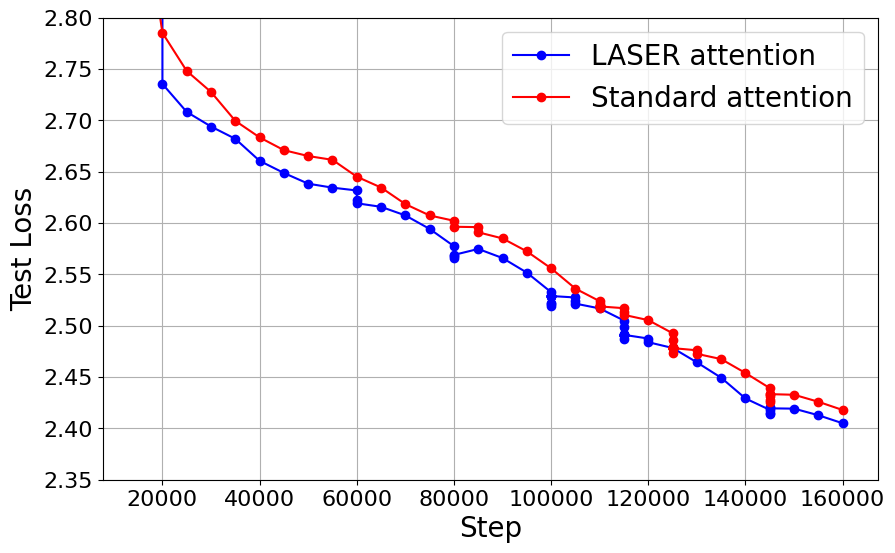
(d) Test loss - 1.1 billion parameter model.

Figure 4: Performance comparison for 2.2 billion and 1.1 billion parameter models. The 2.2 billion model has 32 layers, 8 attention heads with head size 512, MLP hidden dimension 8192, and model dimension 2048. The 1.1 billion model has 32 layers, 8 attention heads (head size 256), MLP hidden dimension 4096, and model dimension 1024. LASER demonstrates better train and test loss compared to Standard Attention even in large scale setting.

Training and evaluation.

All experiments are conducted using the PAX framework (Google, 2023) built on JAX (Bradbury et al., 2018), and executed on TPUv5 chips (Cloud, 2023). We use 64 chips for 300 million parameter model, 128 chips for 1.1 billion and 256 chips for 2.2 billion parameter model. Each training run takes upto 24 hours. We conducted hyperparameter search on 16-layer model mentioned in Table 1 with 15 hyperparameters using search space mentioned in Table 4 and use the optimal hyperparameter for larger models.

4.2 Masked Language Modeling via BERT

In the experiments so far, the focus was mainly on decoder-only models, to diversify our evaluation we now shift to encoder-only model- BERT (Devlin et al., 2018) trained via masked language modeling (as opposed to next token prediction in Section 4.1). We train a 2.2 billion parameter BERT on MLPerf training data which uses wikipedia articles (MLCommons, ). We used model dimension of 2048, hidden dimension - 8192, number of attention heads 16, each of size 256. We get better error rate of masked language model predictions - LASER - 0.2125 vs Standard Attention - 0.2145 (0.93% relative improvement). One can note that LASER shows more improvement in autoregressive language modeling compared to BERT.

4.3 Vision Transformer (ViT) and Conformer - Speech-to-Text

Vision Transformer (ViT) on Imagenet-1k.

In this section, we experiment with the Vision Transformer (ViT) (Dosovitskiy et al., 2021) variant - S/16 on the Imagenet-1k classification task (Deng et al., 2009) which is a part of AlgoPerf benchmarks (Dahl et al., 2023) for optimizer comparisons. These benchmarks are identically implemented in init2winit framework (Gilmer et al., 2023), build on JAX, which we use for our experiments. A hyperparameter sweep was conducted over 50 configurations on NAdamW (Dozat, 2016), focusing on the search space defined in Table 3. We selected the best-performing hyperparameter configuration based on validation performance for standard attention, run it for 5 different random seeds (for initialization) and report the validation curves corresponding to median in Figure 5, where we show that LASER attention provides a 1.15% absolute improvement in error rate (25.27% $\to$ 24.12%), i.e., a $\sim$4% relative improvement over standard attention.

Conformer on Librispeech Speech-to-Text.

We also evaluate the performance of LASER attention on the Librispeech Speech-to-Text dataset (Panayotov et al., 2015) using the Conformer model (Gulati et al., 2020). Similar to the ViT experiments, we use the AlgoPerf benchmark and perform a hyperparameter sweep across 50 configurations to optimize standard attention. We pick the optimal hyperparameters, run them for 5 different random seeds (for initialization) and report the validation curves corresponding to median in Figure 5 where we demonstrate a clear reduction in word error rate (WER) (0.0843 $\to$ 0.0824) when using LASER attention.

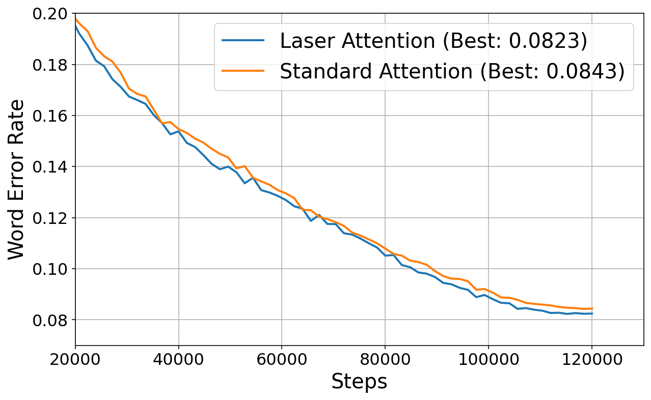
(a) Conformer Speech-to-Text - Validation

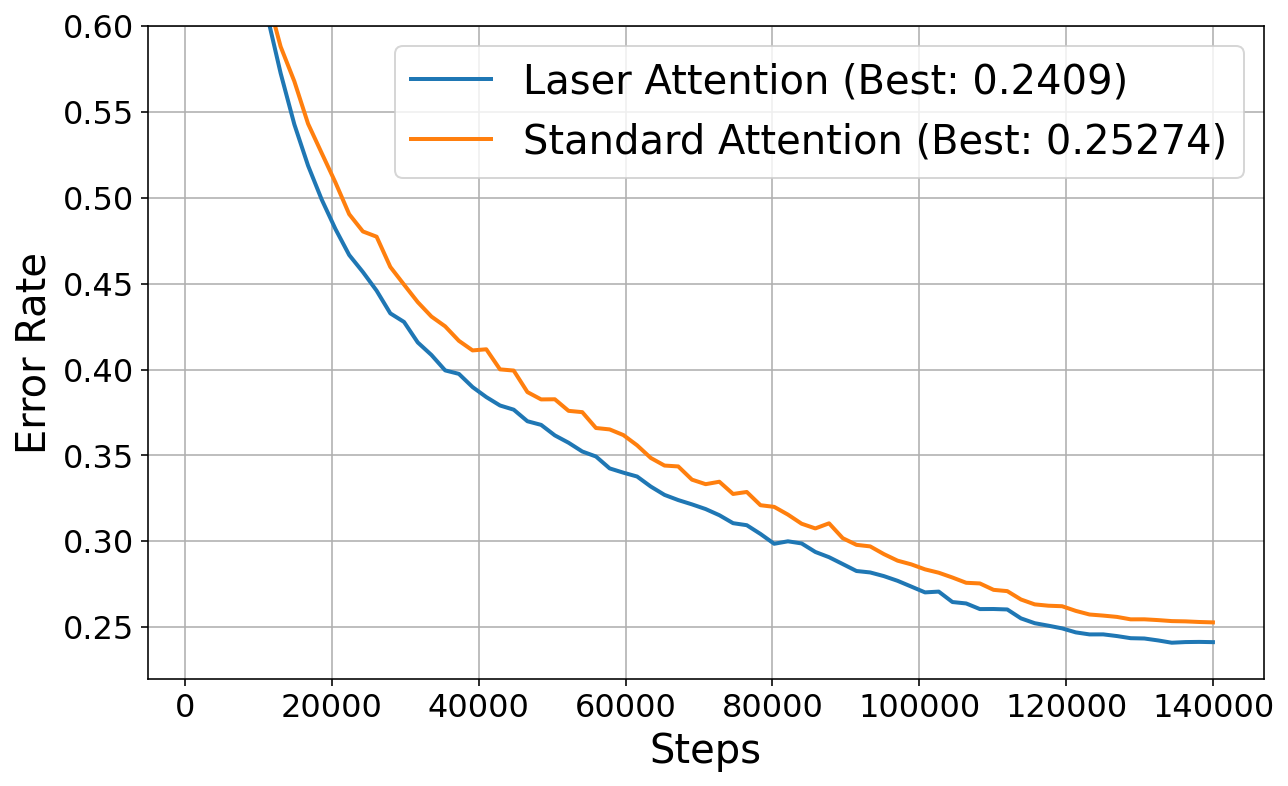
(b) ViT ImageNet Classification - Validation

Figure 5: Comparison of LASER attention vs Standard attention in two tasks: Conformer Speech-to-Text (left) and ViT ImageNet Classification (right). LASER attention provides a 1% absolute improvement in error rate (25.27% $\to$ 24.09%) i.e., a $\sim$4.67% relative improvement. In Conformer, we notice an improvement of word error rate (WER) (0.0843 $\to$ 0.0824) - 2.25% relative improvement. Median curve among 5 random initializations corresponding to the best performing hyperparameter configuration is reported.

Comparisons using OPTLists. In AlgoPerf (Dahl et al., 2023), a list of 5 hyperparameters for NAdamW, tuned for a variety of benchmarks (as opposed to just Conformer and ViT) were provided - OPTList. We also evaluate our models on OPTList by running each hyperparameter with 5 different random seeds (initializations) and picking the median of the best performing hyperparameter. For Imagenet-ViT benchmark we obtain a reduction in validation error rate from 0.21732 to 0.21348. In Librispeech-Conformer benchmark we obtain a reduction in validation word error rate from 0.07728 to 0.07607.

5 Conclusions

In this paper, we first identified a bottleneck in the gradient backpropagation of attention mechanism where the gradients are scaled by small Jacobian values while passing through the softmax operation. We fix this issue by transforming the inputs and outputs of attention mechanism, and show that this leads to larger Jacobians in the limiting case. We demonstrate the improvements in training performance over four types of Transformers spanning different modalities (text, speech and vision): (a) decoder-only (via Large Language model) upto 2.2 billion parameters, (b) encoder-only (BERT) with 2.2 billion parameters, (c)  vision Transformers on Imagenet, and (d) Conformer on Librispeech speech-to-text, where we show significant and consistent improvements in performance.

6 Limitations

Research on novel attention methods have wide applicability, however, due to the quadratic complexity in sequence length, scaling to large sequence lengths can be a major limitation of attention methods.

Appendix A Appendix

A.1 Hyperparameter search space

In Table 3 we outline the hyperparameter search space for all the benchmarks in Section 4.3.

Parameter	Min	Max	Scaling/Feasible Points
learning_rate	$10^{-4}$	$10^{-2}$	log
$1-\beta_{1}$	$10^{-2}$	0.15	log
$\beta_{2}$	-	-	0.9, 0.99, 0.999
warmup_factor	-	-	0.05
weight_decay	$5\times 10^{-3}$	1.0	log
label_smoothing	-	-	0.1, 0.2
dropout_rate	-	-	0.1

Table 3: Hyperparameter search space used in Section 4.3.

Parameter	Value
learning_rate	[1e-1, 1e-2, 1e-3, 1e-4, 1e-5]
weight_decay	[1e-2, 1e-1, 1.0]
beta_1	0.9
beta_2	0.99
epsilon	1e-24
dropout_rate	0.0

Table 4: Hyperparameter search space for language modeling experiments, Section 4.1

A.2 Proofs

Proof of Lemma 3.1. The softmax activation function is applied row-wise on the preactivations $\tilde{A}$; we can expand this computation row-wise as follows:

$$A =\operatorname{softmax}(\tilde{A})$$

$$\implies\begin{pmatrix}{a}_{1}^{\top}\\ \vdots\\ {a}_{s}^{\top}\end{pmatrix} =\begin{pmatrix}\operatorname{softmax}(\tilde{{a}}_{1}^{\top})\\ \vdots\\ \operatorname{softmax}(\tilde{{a}}_{s}^{\top})\end{pmatrix}$$

$$\implies{a}_{i} =\operatorname{softmax}(\tilde{{a}}_{i}),\ \ i\in\{1,\ldots,N\}$$

$$=\left\{\frac{\exp(\tilde{a}_{i1})}{\sum_{k}\exp(\tilde{a}_{ik})},\ldots,\frac{\exp(\tilde{a}_{is})}{\sum_{k}\exp(\tilde{a}_{ik})}\right\}$$

$$\implies a_{ij} =\frac{\exp(\tilde{a}_{ij})}{\sum_{k}\exp(\tilde{a}_{ik})}$$

Taking gradient with respect to $\tilde{a}_{i}$ in the last expression gives:

$$\frac{\partial a_{ij}}{\partial\tilde{a}_{il}} =a_{ij}(1-a_{ij})\ \ \text{if }l=j$$

$$=-a_{ij}a_{il}\ \ \text{else}$$

Putting everything together, the Jacobian of the transformation ${a}_{i}=\operatorname{softmax}(\tilde{{a}}_{i})$ can be written as follows:

$$\frac{\partial{a}_{ij}}{\partial\tilde{{a}}_{il}} =(\operatorname{diag}({a}_{i})-{a}_{i}{a}_{i}^{\top})$$

$$\frac{\partial\ell}{\partial{\tilde{{a}}_{i}}} =(\operatorname{diag}({a}_{i})-{a}_{i}{a}_{i}^{\top})\frac{\partial\ell}{\partial{{{a}}_{i}}}$$ (10)

References

- Ba et al. (2016) Jimmy Lei Ba, Jamie Ryan Kiros, and Geoffrey E Hinton. Layer normalization. arXiv preprint arXiv:1607.06450, 2016.
- Bahdanau et al. (2015) Dzmitry Bahdanau, Kyunghyun Cho, and Yoshua Bengio. Neural machine translation by jointly learning to align and translate. In 3rd International Conference on Learning Representations, ICLR 2015, 2015. URL https://arxiv.org/abs/1409.0473.
- Beltagy et al. (2020) Iz Beltagy, Matthew E Peters, and Arman Cohan. Longformer: The long-document transformer. arXiv preprint arXiv:2004.05150, 2020. URL https://arxiv.org/abs/2004.05150.
- Bengio et al. (1994) Yoshua Bengio, Patrice Simard, and Paolo Frasconi. Learning long-term dependencies with gradient descent is difficult. IEEE Transactions on Neural Networks, 5(2):157–166, 1994.
- Bisk et al. (2020) Yonatan Bisk, Rowan Zellers, Ronan Le Bras, Jianfeng Gao, and Yejin Choi. Piqa: Reasoning about physical commonsense in natural language. In Proceedings of the Thirty-Fourth AAAI Conference on Artificial Intelligence, 2020.
- Blanchard et al. (2019) Pierre Blanchard, Desmond J Higham, and Nicholas J Higham. Accurate computation of the log-sum-exp and softmax functions. arXiv preprint arXiv:1909.03469, 2019.
- Boyd & Vandenberghe (2004) Stephen Boyd and Lieven Vandenberghe. Convex optimization. Cambridge university press, 2004.
- Bradbury et al. (2018) James Bradbury, Roy Frostig, Peter Hawkins, Matthew James Johnson, Chris Leary, and Dougal Maclaurin. JAX: Autograd and XLA. https://github.com/google/jax, 2018. Accessed: 2024-09-25.
- Bridle (1990) John S Bridle. Probabilistic interpretation of feedforward classification network outputs, with relationships to statistical pattern recognition. In Neurocomputing: Algorithms, architectures and applications, pp. 227–236. Springer, 1990.
- Brown et al. (2020) Tom B Brown, Benjamin Mann, Nick Ryder, Melanie Subbiah, Jared Kaplan, Prafulla Dhariwal, Arvind Neelakantan, Pranav Shyam, Girish Sastry, Amanda Askell, Sandhini Agarwal, Ariel Herbert-Voss, Gretchen Krueger, Tom Henighan, Rewon Child, Aditya Ramesh, Daniel M Ziegler, Jeffrey Wu, Clemens Winter, Christopher Hesse, Mark Chen, Eric Sigler, Mateusz Litwin, Scott Gray, Benjamin Chess, Jack Clark, Christopher Berner, Sam McCandlish, Alec Radford, Ilya Sutskever, and Dario Amodei. Language models are few-shot learners. arXiv preprint arXiv:2005.14165, 2020.
- Child et al. (2019) Rewon Child, Scott Gray, Alec Radford, and Ilya Sutskever. Generating long sequences with sparse transformers. arXiv preprint arXiv:1904.10509, 2019. URL https://arxiv.org/abs/1904.10509.
- Cho (2014) Kyunghyun Cho. Learning phrase representations using rnn encoder-decoder for statistical machine translation. arXiv preprint arXiv:1406.1078, 2014.
- Choromanski et al. (2021) Krzysztof Choromanski, Valerii Likhosherstov, David Dohan, Xingyou Song, Andreea Gane, Tamas Sarlos, Peter Hawkins, Jared Q Davis, Afroz Mohiuddin, Łukasz Kaiser, et al. Rethinking attention with performers. In International Conference on Learning Representations, 2021.
- Clark et al. (2019) Christopher Clark, Kenton Lee, Ming-Wei Chang, Tom Kwiatkowski, Michael Collins, and Kristina Toutanova. Boolq: Exploring the surprising difficulty of natural yes/no questions. In Proceedings of the 2019 Conference of the North American Chapter of the Association for Computational Linguistics: Human Language Technologies, 2019.
- Clark et al. (2018) Peter Clark, Isaac Cowhey, Oren Etzioni, Tushar Khot, Ashish Sabharwal, Caroline Schoenick, and Oyvind Tafjord. Think you have solved question answering? try arc, the ai2 reasoning challenge. arXiv preprint arXiv:1803.05457, 2018.
- Cloud (2023) Google Cloud. Google cloud tpu v5e: Next-generation ai hardware for large-scale model training. https://cloud.google.com/blog/products/ai-machine-learning/introducing-tpu-v5e, 2023. Accessed: 2024-09-25.
- Dahl et al. (2023) George E Dahl, Frank Schneider, Zachary Nado, Naman Agarwal, Chandramouli Shama Sastry, Philipp Hennig, Sourabh Medapati, Runa Eschenhagen, Priya Kasimbeg, Daniel Suo, et al. Benchmarking neural network training algorithms. arXiv preprint arXiv:2306.07179, 2023.
- Dao & Gu (2024) Tri Dao and Albert Gu. Transformers are ssms: Generalized models and efficient algorithms through structured state space duality. arXiv preprint arXiv:2405.21060, 2024.
- Dao et al. (2022) Tri Dao, Daniel Y Fu, Stefano Ermon, Atri Rudra, and Christopher Ré. Flashattention: Fast and memory-efficient exact attention with io-awareness. Advances in Neural Information Processing Systems, 2022. URL https://arxiv.org/abs/2205.14135.
- Dao et al. (2024) Tri Dao, Daniel Fu, Xinyang G Wang, et al. Flashattention 2: Faster attention with better memory scheduling. arXiv preprint arXiv:2401.14155, 2024. URL https://arxiv.org/abs/2401.14155.
- Deng et al. (2009) Jia Deng, Wei Dong, Richard Socher, Li-Jia Li, Kai Li, and Li Fei-Fei. Imagenet: A large-scale hierarchical image database. In 2009 IEEE conference on computer vision and pattern recognition, pp. 248–255. Ieee, 2009.
- Devlin et al. (2018) Jacob Devlin, Ming-Wei Chang, Kenton Lee, and Kristina Toutanova. Bert: Pre-training of deep bidirectional transformers for language understanding. arXiv preprint arXiv:1810.04805, 2018.
- Dosovitskiy et al. (2021) Alexey Dosovitskiy, Lucas Beyer, Alexander Kolesnikov, Dirk Weissenborn, Xiaohua Zhai, Thomas Unterthiner, Mostafa Dehghani, Matthias Minderer, Georg Heigold, Sylvain Gelly, et al. An image is worth 16x16 words: Transformers for image recognition at scale. arXiv preprint arXiv:2010.11929, 2021.
- Dozat (2016) Timothy Dozat. Incorporating nesterov momentum into adam. 2016.
- Dubey et al. (2024) Abhimanyu Dubey, Abhinav Jauhri, Abhinav Pandey, Abhishek Kadian, Ahmad Al-Dahle, Aiesha Letman, Akhil Mathur, Alan Schelten, Amy Yang, Angela Fan, et al. The llama 3 herd of models. arXiv preprint arXiv:2407.21783, 2024.
- Gemini (2024) Team Gemini. Gemini 1.5: Unlocking multimodal understanding across millions of tokens of context. arXiv preprint arXiv:2403.05530, 2024. URL https://arxiv.org/abs/2403.05530.
- Gilmer et al. (2023) Justin M. Gilmer, George E. Dahl, Zachary Nado, Priya Kasimbeg, and Sourabh Medapati. init2winit: a jax codebase for initialization, optimization, and tuning research, 2023. URL http://github.com/google/init2winit.
- Glorot & Bengio (2010) Xavier Glorot and Yoshua Bengio. Understanding the difficulty of training deep feedforward neural networks. In Proceedings of the thirteenth international conference on artificial intelligence and statistics, pp. 249–256. JMLR Workshop and Conference Proceedings, 2010.
- Google (2023) Research Google. Pax: A JAX-based neural network training framework. https://github.com/google/paxml, 2023. Accessed: 2024-09-25.
- Gu & Dao (2023) Albert Gu and Tri Dao. Mamba: Linear-time sequence modeling with selective state spaces. arXiv preprint arXiv:2312.00752, 2023.
- Gulati et al. (2020) Anmol Gulati, James Qin, Chung-Cheng Chiu, Niki Parmar, Yu Zhang, Jiahui Yu, Wei Han, Shibo Wang, Zhengdong Zhang, Yonghui Wu, et al. Conformer: Convolution-augmented transformer for speech recognition. In Proc. Interspeech, 2020.
- He et al. (2016) Kaiming He, Xiangyu Zhang, Shaoqing Ren, and Jian Sun. Deep residual learning for image recognition. In Proceedings of the IEEE conference on computer vision and pattern recognition, pp. 770–778, 2016.
- Hochreiter & Schmidhuber (1997) Sepp Hochreiter and Jürgen Schmidhuber. Long short-term memory. Neural computation, 9(8):1735–1780, 1997.
- Katharopoulos et al. (2020) Angelos Katharopoulos, Apoorv Vyas, Nikolaos Pappas, and François Fleuret. Transformers are RNNs: Fast autoregressive transformers with linear attention. In International conference on machine learning, pp. 5156–5165. PMLR, 2020.
- Khashabi et al. (2018) Daniel Khashabi, Snigdha Chaturvedi, Michael Roth, Shyam Upadhyay, and Dan Roth. Looking beyond the surface: A challenge set for reading comprehension over multiple sentences. Proceedings of the 2018 Conference of the North American Chapter of the Association for Computational Linguistics: Human Language Technologies, pp. 252–262, 2018.
- Kocijan et al. (2020) Vid Kocijan, Elias Chamorro-Perera, Damien Sileo, Jonathan Raiman, and Peter Clark. Winogrande: An adversarial winograd schema challenge at scale. In Proceedings of the AAAI Conference on Artificial Intelligence, volume 34, pp. 8732–8740, 2020.
- Lai et al. (2017) Guokun Lai, Qizhe Xie, Hanxiao Liu, Yiming Yang, and Eduard Hovy. Race: Large-scale reading comprehension dataset from examinations. In Proceedings of the 2017 Conference on Empirical Methods in Natural Language Processing, pp. 785–794, 2017.
- LeCun et al. (2002) Yann LeCun, Léon Bottou, Genevieve B Orr, and Klaus-Robert Müller. Efficient backprop. In Neural networks: Tricks of the trade, pp. 9–50. Springer, 2002.
- Levesque et al. (2012) Hector J. Levesque, Ernest Davis, and Leora Morgenstern. The winograd schema challenge. In Proceedings of the Thirteenth International Conference on Principles of Knowledge Representation and Reasoning, pp. 552–561, 2012.
- Liu et al. (2023) Hao Liu, Matei Zaharia, and Pieter Abbeel. Ring attention with blockwise transformers for near-infinite context. arXiv preprint arXiv:2310.01889, 2023.
- Loshchilov & Hutter (2016) Ilya Loshchilov and Frank Hutter. Sgdr: Stochastic gradient descent with warm restarts. arXiv preprint arXiv:1608.03983, 2016.
- Loshchilov & Hutter (2017) Ilya Loshchilov and Frank Hutter. Decoupled weight decay regularization. arXiv preprint arXiv:1711.05101, 2017.
- Meta-AI (2024) Team Meta-AI. The llama 3 herd of models. arXiv preprint arXiv:2407.21783, 2024. URL https://arxiv.org/abs/2407.21783.
- Mihaylov et al. (2018) Todor Mihaylov, Peter Clark, Tushar Khot, and Ashish Sabharwal. Can a suit of armor conduct electricity? a new dataset for open book question answering. In Proceedings of the 2018 Conference on Empirical Methods in Natural Language Processing, pp. 2381–2391, 2018.
- (45) MLCommons. Bert dataset documentation. https://github.com/mlcommons/training/blob/master/language_model/tensorflow/bert/dataset.md. Accessed: 2024-10-16.
- Mostafazadeh et al. (2016) Nasrin Mostafazadeh, Nathanael Chambers, Xiaodong He, Devi Parikh, Dhruv Batra, Lucy Vanderwende, Pushmeet Kohli, and James Allen. A corpus and cloze evaluation for deeper understanding of commonsense stories. In Proceedings of the 2016 Conference of the North American Chapter of the Association for Computational Linguistics: Human Language Technologies, pp. 839–849, 2016.
- Panayotov et al. (2015) Vassil Panayotov, Guoguo Chen, Daniel Povey, and Sanjeev Khudanpur. Librispeech: An asr corpus based on public domain audio books. In 2015 IEEE International Conference on Acoustics, Speech and Signal Processing (ICASSP), pp. 5206–5210. IEEE, 2015.
- Pilehvar & Camacho-Collados (2019) Mohammad Taher Pilehvar and Jose Camacho-Collados. Wic: The word-in-context dataset for evaluating context-sensitive meaning representations. In Proceedings of the 2019 Conference of the North American Chapter of the Association for Computational Linguistics: Human Language Technologies, Volume 1 (Long and Short Papers), pp. 1267–1273, 2019.
- Radford et al. (2018) Alec Radford, Karthik Narasimhan, Tim Salimans, and Ilya Sutskever. Improving language understanding by generative pre-training. 2018. OpenAI.
- Raffel et al. (2020) Colin Raffel, Noam Shazeer, Adam Roberts, Katherine Lee, Sharan Narang, Michael Matena, Yanqi Zhou, Wei Li, and Peter J. Liu. Exploring the limits of transfer learning with a unified text-to-text transformer. In Journal of Machine Learning Research, volume 21, pp. 1–67, 2020. URL http://jmlr.org/papers/v21/20-074.html.
- Roy et al. (2021) Aurko Roy, Mohammad Saffar, Ashish Vaswani, and David Grangier. Efficient routing transformers: Dynamic token interaction models for natural language processing. arXiv preprint arXiv:2003.05997, 2021. URL https://arxiv.org/abs/2003.05997.
- Vaswani et al. (2017) Ashish Vaswani, Noam Shazeer, Niki Parmar, Jakob Uszkoreit, Llion Jones, Aidan N Gomez, Łukasz Kaiser, and Illia Polosukhin. Attention is all you need. In Advances in neural information processing systems, volume 30, 2017.
- Wang et al. (2019) Alex Wang, Yada Pruksachatkun, Nikita Nangia, Amanpreet Singh, Julian Michael, Felix Hill, Omer Levy, and Samuel R Bowman. Superglue: A stickier benchmark for general-purpose language understanding systems. In Advances in Neural Information Processing Systems (NeurIPS), pp. 3261–3275. Curran Associates, Inc., 2019.
- Xiong et al. (2020) Ruibin Xiong, Yingquan Yang, Di He, Kai Zheng, Shuxin Zheng, Yaliang Lan, Jingdong Wang, and Tie-Yan Liu. On layer normalization in the transformer architecture. In International Conference on Machine Learning, pp. 10524–10533. PMLR, 2020.
- You et al. (2019) Yang You, Jing Li, Sashank Reddi, Jason Hseu, Sanjiv Kumar, Srinadh Bhojanapalli, Xiaodan Song, James Demmel, and Cho-Jui Hsieh. Large batch optimization for deep learning: Training bert in 76 minutes. arXiv preprint arXiv:1904.00962, 2019.
- Zellers et al. (2019) Rowan Zellers, Ari Holtzman, Yonatan Bisk, Ali Farhadi, and Yejin Choi. Hellaswag: Can a machine really finish your sentence? In Proceedings of the 57th Annual Meeting of the Association for Computational Linguistics, pp. 4791–4800, 2019.
- Zhang et al. (2018) Shuailong Zhang, Huanbo Liu, Shuyan Liu, Yuwei Wang, Jiawei Liu, Zhiyu Gao, Wei Xu, Yiming Xu, Xin Sun, Lei Cui, et al. Record: Bridging the gap between human and machine commonsense reading comprehension. arXiv preprint arXiv:1810.12885, 2018.