Constraining accretion physics with gravitational waves from
eccentric extreme-mass-ratio inspirals

Abstract

We study the evolution of eccentric, equatorial extreme-mass-ratio inspirals (EMRIs) immersed in the accretion disks of active galactic nuclei. We find that single gravitational-wave observations from these systems could provide measurements with $\sim 10\%$ relative precision of, simultaneously, the disk viscosity and mass accretion rate of the central supermassive black hole. This is possible when the EMRI transitions, within the observation time, from supersonic to subsonic motion relative to the disk gas, for eccentricities $e\gtrsim 0.025-0.1$. The estimate of the accretion rate would assist in the identification of the EMRI’s host galaxy, or the observation of a direct electromagnetic counterpart, improving the chances of using these sources as cosmological sirens. Our work highlights the rich phenomenology of binary evolution in astrophysical environments and the need to improve the modelling and analysis of these systems for future gravitational-wave astronomy.

I Introduction

The role that astrophysical environments play in binary coalescences has gained increasing attention in recent years. Accretion disks Kocsis et al. (2011); Barausse et al. (2014); Derdzinski et al. (2021); Zwick et al. (2021a, 2022); Speri et al. (2022a); Caputo et al. (2020); Garg et al. (2022); Barausse and Rezzolla (2008); Duffell et al. (2024); Zwick et al. (2024), dark matter distributions Speeney et al. (2022); Cardoso et al. (2022a, b); Brito and Shah (2023); Cannizzaro et al. (2023); Destounis et al. (2023); Baumann et al. (2022a, b); Tomaselli et al. (2023); Bamber et al. (2023); Aurrekoetxea et al. (2023); Tomaselli et al. (2024); Duque et al. (2023); Tomaselli et al. (2024); Bošković et al. (2024) and third-body companions Cardoso et al. (2021a); Gupta et al. (2020); Suzuki et al. (2020); Sberna et al. (2022); Gupta et al. (2022); Oancea et al. (2023); Maeda et al. (2023); Zwick et al. (2024); Yin et al. (2024) all lead to distinctive features in the trajectory of a binary, and, consequently, in its gravitational wave (GW) signature Cole et al. (2023); Zwick et al. (2022); Kejriwal et al. (2023); Santoro et al. (2024).

Extreme-mass-ratio inspirals (EMRIs) are particularly prone to environmental effects. EMRIs are composed by a secondary stellar-mass compact object, typically a black hole (BH) with $\sim 10-100\,M_{\odot}$, orbiting around a primary supermassive black hole (SMBH) with $\gtrsim 10^{5}\,M_{\odot}$. They are one of the main scientific targets of the Laser Interferometer Space Antenna (LISA) Babak et al. (2017); Amaro-Seoane et al. (2023); Arun et al. (2022); Afshordi et al. (2023); Colpi et al. (2024), a space-based GW interferometer sensitive to the mHz frequency band, which has recently been adopted by the European Space Agency and is currently planned to be launched in 2035. EMRIs will complete thousands of orbital cycles while in the LISA observation window. Even small deviations from vacuum general relativity (GR), like the ones introduced by the presence of an environment, can become distinguishable when accumulated over so many orbits Speri et al. (2022a); Cole et al. (2023); Barsanti et al. (2023); Kejriwal et al. (2023); Speri et al. (2024).

Most studies of environmental effects for LISA sources have been restricted to circular orbits. However, EMRIs formed via multibody scattering in dense nuclear clusters are expected to enter the observation band with a large eccentricity and retain it up to coalescence Babak et al. (2017); Bonetti and Sesana (2020); Vázquez-Aceves et al. (2022). The interaction with gas-rich environments, like the accretion disk of an active galactic nucleus (AGN), also assists EMRI formation and increases their rates per SMBH by orders of magnitude Pan et al. (2021); Pan and Yang (2021); Wang et al. (2022); Derdzinski and Mayer (2022). In fact, the collision between the secondary and the disk may be the mechanism behind the dozen of Quasi-Periodic Eruptions/Oscillations recently observed in the soft X-ray band ($0.1\,\text{keV}$) Kejriwal et al. (2024); Linial and Metzger (2023); Franchini et al. (2023); Arcodia et al. (2024); Zajaček et al. (2024). EMRIs formed via this wet channel are expected to be equatorial and have negligible eccentricities when entering the LISA band Tanaka et al. (2002); Tanaka and Ward (2004); Pan et al. (2021); Pan and Yang (2021); Zwick et al. (2021b). However, eccentricity damping might be reduced when considering the entire evolution history of these EMRIs, e.g., when considering interactions with other compact bodies or disk turbulence, or the fact that accretion by the SMBH can have quiescent periods where the disk density is smaller Cardoso et al. (2021b); Hu et al. (2023); Zwick et al. (2021a); Gupta et al. (2020); Suzuki et al. (2020); Gupta et al. (2022); Oancea et al. (2023); Maeda et al. (2023); Nelson (2005); Johnson et al. (2006); Yang et al. (2009); Szölgyén et al. (2022); Breslau and Pfalzner (2019); Franchini et al. (2024); Tomaselli et al. (2024); Wang et al. (2024); Wu et al. (2023); Ogihara et al. (2007); Wang et al. (2024). LISA is expected to measure the eccentricity of EMRIs at coalescence with absolute precision of $~{}10^{-5}$ Babak et al. (2017); Colpi et al. (2024), so it is timely to extend studies of these environmental effects to eccentric inspirals.

An EMRI evolving in an AGN disk is subject to several effects Binney and Tremaine (2011): mass accretion by both the primary and the secondary Bondi and Hoyle (1944); Bondi (1952); Kocsis et al. (2011); Barausse et al. (2014); axisymmetric gravitational effects from the disk’s self gravity Kocsis et al. (2011); Barausse et al. (2014); hydrodynamical drag induced by the relative velocity between the secondary and the gas in the disk Barausse and Rezzolla (2008); Kocsis et al. (2011); Barausse et al. (2014); dynamical friction by a density wake generated by the secondary’s gravity, which then trails behind the secondary and exerts an additional gravitational pull on it Chandrasekhar (1943); Ostriker (1999); Vicente et al. (2019). For a circular binary, this wake forms a spiral density wave assisted by the disk’s differential rotation, which can resonantly exchange angular momentum with the secondary Goldreich and Tremaine (1980); Tanaka et al. (2002); Tanaka and Ward (2004); Kocsis et al. (2011); Hirata (2011a, b); Muto et al. (2011); Ida et al. (2020); Gilbaum et al. (2024). This effect is analogous to (planetary) migration in protoplanetary disks.

Past work showed that of all the effects listed above, migration is the most relevant for quasicircular EMRIs where the secondary is embedded in an AGN disk Kocsis et al. (2011); Barausse et al. (2014); Speri et al. (2022a). Using state-of-the-art waveform models for EMRIs Chua et al. (2021); Katz et al. (2021) and a Bayesian framework for parameter estimation, Speri et al. Speri et al. (2022a) prospected that LISA can measure migration torques in different accretion scenarios and impose constraints on the disk properties (e.g. viscosity, accretion rate), if GW observations are combined with multimessenger electromagnetic counterparts. If migration is neglected in the analysis of these systems, one incurs in biases in the mass and spin of the primary that may jeopardize tests of fundamental physics and lead to false deviations from GR Kejriwal et al. (2023).

However, migration arises from resonances between the secondary’s orbital frequency and epicyclic motion at different radii of the disk. This is a global effect, where one needs to consider density/temperature gradients along the extended gas distribution. As eccentricity increases, these resonances become less effective Zwick et al. (2021b); Muto et al. (2011); Ida et al. (2020). In fact, binaries with eccentricities $e\gtrsim 0.025-0.1$ become supersonic relative to the (local) gas in the disk. The transition from subsonic to supersonic motion alters the nature of the secondary-disk interactions. Dynamical friction from the local gas is very weak in the subsonic regime because the wakes in front and behind the secondary are almost symmetric, which cancels their net effect. Rephaeli and Salpeter (1980); Ostriker (1999); Vicente et al. (2019). As the secondary transitions to the supersonic regime, this symmetry is broken, the spiral structure typical of migration does not form, and local dynamical friction becomes the dominant environmental effect Papaloizou and Larwood (2000); Cresswell and Nelson (2008); Bitsch and Kley (2010); Muto et al. (2011); Ida et al. (2020); Sánchez-Salcedo (2019, 2020).

In this work, we extend the study of EMRIs in accretion flows to eccentric orbits, equatorial and prograde with respect to the motion of the gas in the disk. In Section II, we construct a phenomenological model describing the secular correction in the secondary’s trajectory due to the interactions with the gas environment, including the eccentricity evolution. Our model is inspired by previous explorations in the context of planetary migration, where hydrodynamical simulations are used to match analytic estimates in both the subsonic and supersonic limit Muto et al. (2011); Ida et al. (2020); Sánchez-Salcedo (2019). As we will see, in the supersonic regime, eccentricity damping is weakened, and its typical evolution timescale becomes larger than the inspiralling timescale.

We implement our model in the state-of-the-art FastEMRIWaveform (few) package for EMRI waveform computation Chua et al. (2021); Katz et al. (2021); Speri et al. (2023) and use a Fisher-Matrix framework to study inference with LISA in Section III.1. We find that eccentricity typically helps to probe the astrophysical environment of the EMRI, even for values as small as $e_{0}\sim 0.01$ at the start of the observation. Moreover, it allows for independent measurements of both disk viscosity and the primary mass accretion rate, without the need for an electromagnetic counterpart, something that was not possible for circular motion. We also comment, in Section III.2 and III.3, on the implications of our results for EMRI formation in gaseous environments, and multimessenger astronomy with EMRIs, respectively. Finally, in Section IV we discuss the limitations of our work and identify challenges for the future. Unless stated otherwise, we adopt geometric units with $G=c=1$.

II Methods

In this Section, we summarize the adopted disk model and construct a phenomological model for the interaction of the EMRI with the disk environment, valid up to large eccentricities. We also describe how to implement these effects in few for waveform evaluation and the Fisher-matrix framework used for inference.

II.1 Accretion-disk model

We denote the mass of the primary central BH by $M$ and the mass of the secondary compact body by $\mu$. Following Refs. Zwick et al. (2021a); Derdzinski et al. (2021), we consider a Newtonian, radiatively-efficient, stationary, thin-accretion disk, that is accreted by the central SMBH at a steady-state rate

$$\dot{M}\sim 3\pi\nu\Sigma\sim\text{constant}\,,$$ (1)

with $\Sigma$ the disk’s surface density and $\nu$ its kinematic viscosity. The viscosity is taken to be parametrized by a constant $\alpha$, such that $\nu=\alpha c_{s}H$, where $H$ is the disk scale height, $c_{s}=H\Omega_{K}$ the isothermal sound speed, and $\Omega_{K}=\sqrt{M/r^{3}}$ the Keplerian orbital frequency. The disk density is then $\rho=\Sigma/2H$ and the thin-disk approximation needs to satisfy $2H\ll r$ (this is verified throughout the evolution of the EMRI).

We parameterize the disk profile according to a power law for the surface density $\Sigma(r)$ and the aspect ratio $h(r)$

$$\Sigma(r) = \Sigma_{0}\left(\frac{r}{10M}\right)^{-\Sigma_{p}}\,,$$ (2)

$$h(r) = \frac{H(r)}{r}=h_{0}\left(\frac{r}{10M}\right)^{(2\Sigma_{p}-1)/4}\,,$$ (3)

where $\Sigma_{p}\in\mathbb{Z}$, $\Sigma_{0}$ and $h_{0}$ are typical values in the inner region of the disk, and the power appearing in $h(r)$ ensures the primary accretes mass at a constant rate. We adopt this parameterization since it allows to quickly identify when the secondary is in the subsonic or supersonic regime by comparing the orbit’s eccentricity $e$ with $h_{0}$.

Our disk model reformulates the Shakura-Sunayev $\alpha$-model Shakura and Sunyaev (1973); Abramowicz and Fragile (2013); Frank et al. (2002); Derdzinski and Mayer (2022), which captures the general features observed in magnetohydrodynamic simulations of turbulent, radiatively-efficient disks Nouri and Janiuk (2023); Chen et al. (2023); Gangardt et al. (2024). The $\alpha$-disk model takes the viscous stress to be proportional to the total pressure in the disk, i.e. $t_{r\varphi}=\alpha\left(p_{\text{gas}}+p_{\text{rad}}\right)$, where $p_{\text{gas}}$ is the thermal gas pressure and $p_{\text{rad}}$ is the radiation pressure. Observations and numerical simulations indicate that in the disk’s inner region ($r\lesssim 10^{2}M$), pressure is dominated by radiation and opacity by electron scattering Bell and Lin (1994); Sirko and Goodman (2003); Derdzinski and Mayer (2022). Under these assumptions Shakura and Sunyaev (1973); Kocsis et al. (2011); Speri et al. (2022a); Garg et al. (2022)

$$\Sigma_{\alpha} \approx 5.4\times 10^{2}\left(\frac{0.1}{\alpha}\right)\left(\frac{0.1}{f_{\text{Edd}}}\frac{\epsilon}{0.1}\right)\Big{(}\frac{r}{10M}\Big{)}^{3/2}\left[\frac{\text{g}}{\text{cm}^{2}}\right]\,,$$

(4)

$$h_{\alpha} \approx 0.15\left(\frac{f_{\text{Edd}}}{0.1}\frac{0.1}{\epsilon}\right)\Big{(}\frac{r}{10M}\Big{)}^{-1}\,.$$ (5)

Here, $f_{\text{Edd}}$ is the ratio of the Eddington rate at which the primary is accreting and $\epsilon$ is the efficiency of conversion of mass-energy to radiation, such that $\dot{M}=f_{\text{Edd}}L_{\text{Edd}}/\epsilon$, with $L_{\text{Edd}}$ the Eddington luminosity. These quantities appear in the disk structure always through the ratio $f_{\text{Edd}}/\epsilon$. Their typical values are $f_{\text{Edd}}\sim 0.01-0.1$, $\epsilon\sim 0.1$, and for the viscosity coefficient $\alpha\sim 0.001-0.1$ Jiang et al. (2019a); Davis et al. (2010); Nouri and Janiuk (2023). These values correspond to $\Sigma\sim 10^{3}-10^{6}\,\text{g}/\text{cm}^{2}$ and $h\sim 0.01-0.1$, which are compatible with current observations Jiang et al. (2019b).

By picking $\Sigma_{p}=-3/2$ in the power-law model (2)-(3), any choice of $\Sigma_{0}$ and $h_{0}$ can then be mapped to a combination of $\alpha$ and $f_{\text{Edd}}/\epsilon$ of the $\alpha$-model. We will focus on this profile in this work, but one can repeat the mapping for any particular disk solution with different physics, like a different opacity law governing a different region of the disk (see Table 1 and Fig. 1 of Ref. Derdzinski and Mayer (2022)) or a different dependence between the viscous stress and pressure. For example, in the $\beta$-disk model, the viscous stress is proportional to only the thermal gas pressure Shakura and Sunyaev (1973); Abramowicz and Fragile (2013); Frank et al. (2002), i.e. $t_{r\varphi}=\alpha p_{\text{gas}}$. This choice cures the thermal instabilities present in the $\alpha$-disk and leads to $\Sigma_{\beta}\propto r^{-3/5}$, but is less favoured by both simulations and observations. Ultimately, we can remain agnostic about the internal physical properties of the disk and ask instead what regions of the parameter space $\left\{\Sigma_{0},\,h_{0},\,\Sigma_{p}\right\}$ lead to distinguishable environmental effects in the GW signature of an EMRI. Though some of them may not directly correspond to known disk solutions, they might still be physically relevant considering all the uncertainties in the astrophysics of AGN disks, the discrepancies between the finer details of numerical simulations and simple analytical models like the $\alpha$-disk, and the time-dependence in the disk structure due to the inspiral of the secondary and instabilities (e.g. turbulence) Jiang et al. (2019a); Nouri and Janiuk (2023); Derdzinski et al. (2021); Gangardt et al. (2024).

We are also ignoring relativistic corrections Novikov and Thorne (1973) and changes at the inner edge of the disk, which would complicate the power-law profiles proposed in Eqs. (2)-(3). Imposing that viscous stress vanish at the disk’s inner edge at some radius $r_{\text{in}}$ introduces corrective factors of

$$F^{4}=1-\sqrt{r_{\text{in}}/r}\,,$$ (6)

up to some power in the disk structure (e.g. $\Sigma_{\alpha}\propto F^{-1}$ and $h_{\alpha}\propto F^{4}$) Shakura and Sunyaev (1973); Kocsis et al. (2011); Speri et al. (2022a); Garg et al. (2022). Since we are mostly interested in how eccentricity affects the interaction of the secondary with the disk, we ignore these corrections.

II.2 Torque model

The relative velocity $\Delta v$ between the secondary and the (local) gas in the disk dictates the nature of their gravitational interaction. For equatorial orbits prograde with respect to the disk rotation

$$\Delta v\approx ev_{K}=er\Omega_{K}=\frac{e}{h}c_{s}\,,$$ (7)

where $v_{K}$ is the Keplerian velocity at radius $r$. Therefore, for $e\lesssim h$, the EMRI is in the subsonic regime and vice-versa Muto et al. (2011); Ida et al. (2020). Considering that $h\gtrsim 0.02$ in the inner disk region, an EMRI can attain supersonic motion even with moderately low eccentricity.

II.2.1 Subsonic motion

In the quasicircular, subsonic regime, the EMRI excites spiral density waves due to the shear motion of the disk gas Goldreich and Tremaine (1980); Tanaka et al. (2002); Tanaka and Ward (2004); Kocsis et al. (2011); Hirata (2011a, b); Muto et al. (2011); Ida et al. (2020). The wake then backreacts on the binary by exerting additional forces/torques, which excite resonances at specific locations in the disk (e.g., Lindblad resonances). As a consequence, the binary “migrates”, either inwards or outwards depending on the net torque between ingoing spiral waves, which transfer angular momentum to the binary, and outgoing ones, which extract angular momentum from it. Migration can be understood as dynamical friction, but takes into account the differential rotation of the disk gas at radii far-away from the secondary. If the secondary is massive enough, it can open a gap in the disk and migration is said to be of Type-II. The EMRIs we will study do not fulfill this condition Kocsis and Loeb (2008); Gilbaum et al. (2024), and thus we consider only Type-I migration.

In general, migration torques act on the inverse timescale

$$\frac{1}{t_{\text{gas}}}=\varepsilon\left(\frac{\Sigma r^{2}}{M}\right)\frac{\Omega_{K}}{h^{4}}\,,$$ (8)

where $\varepsilon=\mu/M$ is the small mass ratio . Ref. Tanaka et al. (2002); Tanaka and Ward (2004) used linear perturbation theory to compute the force felt by the secondary at every location in a slightly eccentric prograde orbit with $e\ll h$, taking into account corotation torques and the 3D structure of the disk (they also included inclination in their analysis, but we focus on equatorial orbits). This force can then be averaged over one period to obtain the timescales for the evolution of the orbital parameters, namely the semi-major axis $a_{\text{m}}$ (or alternatively the semi-lactus rectum $p$) and eccentricity

$$\frac{1}{t^{\text{sub}}_{a_{\text{m}}}} = -\frac{\left<da_{\text{m}}/dt\right>}{a}=2\frac{C_{\text{sub}}}{t_{\text{gas}}}h^{2}\,,$$ (9)

$$\frac{1}{t^{\text{sub}}_{e}} = -\frac{\left<de/dt\right>}{e}=\frac{0.78}{t_{\text{gas}}}\,,$$ (10)

where the radial-dependent quantities are to be evaluated at $a_{\text{m}}$. $C_{\text{sub}}$ is a numerical factor that may depend on the density and temperature gradient of the disk. It is calibrated with hydrodynamical simulations Jiménez and Masset (2017), but these estimates still have uncertainties and do not take into account all features present in AGN disks, such as:

1. Reflections of the wake at the disk’s inner edge, which are expected to weaken the torque when the reflected wave reaches the secondary Tsang (2011); Miranda and Lai (2018);

2. Increase in the surface density, which increases the torques, at the disk’s inner edge introduced by the $F$ factor (6);

3. Magnetic fields, which can generate turbulent flows Comins et al. (2016); Terquem (2003); Fromang et al. (2005); Uribe et al. (2011); Muto et al. (2008); Sanchez-Salcedo (2012), responsible for stochastic torque fluctuations. These can also arise from asymmetries in the gas flow near the secondary Nelson (2005); Johnson et al. (2006); Kley and Nelson (2012); Yang et al. (2009); Derdzinski et al. (2021); Zwick et al. (2021a). Stochastic torques lead to “diffusive” migration similar to a random walk, and typically increase eccentricity and inclination Nelson (2005); Ogihara et al. (2007);

4. Radiative effects from relaxing the disk isothermality condition Jiménez and Masset (2017), which in turn relaxes the relation between the power-law for the aspect ratio (3) and the one for the surface density (2).

5. “Thermal” torques from heat diffusion near the secondary Masset (2017); Hankla et al. (2020); Grishin et al. (2023); Gangardt et al. (2024). In many disk regions, thermal torques have a positive sign and thus lead to outward migration. They can dominate over gravitational torques (and radiation reaction from GWs) in outer regions of the disk ($r\gtrsim 800M$), and even create migration traps, where the net torque felt by the secondary is zero. Thermal torques also typically increase eccentricity and inclination Fromenteau and Masset (2019).

6. Relativistic effects both in the disk structure and wake dynamics Hirata (2011a, b).

The corrections listed above mostly change the value of $C_{\text{sub}}$ by a numerical factor of $\mathcal{O}(1)$. Though this variation can impact parameter estimation, in this work we are more interested in understanding the role that eccentricity plays in the detectability of environmental effects. Thus, to ease comparison with previous works Kocsis and Loeb (2008); Kocsis et al. (2011); Speri et al. (2022a), in the subsonic limit we adopt the value used there

$$C_{\text{sub}}=1.364+0.541\Sigma_{p}\,.$$ (11)

Note that these modeling uncertainties should also correspond to different numerical factors for the amplitude of $1/t_{e}$, but these have been much less explored. We therefore use the most common value found in literature ($0.78$) Tanaka and Ward (2004); Ida et al. (2020).

Finally, as mentioned above, we focus on prograde motion of the secondary with respect to the gas flow in the disk. The evolution timescales for retrograde motion can differ by orders of magnitude Sánchez-Salcedo et al. (2018); Sánchez-Salcedo (2020) – and also lead to eccentricity excitation – but according to formation models, EMRIs immersed in AGN disks will be already prograde when entering the LISA band Wang et al. (2024); Stone et al. (2017); Derdzinski and Mayer (2022).

II.2.2 Supersonic motion

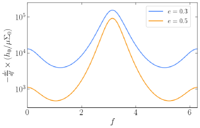
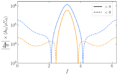
Figure 1: Left: Variation of the eccentricity over one complete orbit due to dynamical friction in the inner region of an $\alpha$-disk ($\Sigma_{p}=-3/2$ for the power-law surface density in Eq. (2)). The secondary is in supersonic motion relative to the gas flow on an orbit with semi-major axis $a_{\text{m}}=10M$. Dynamical friction always acts to circularize the orbit ($de/df<0$ during the whole orbit); Right: same as the left panel but for the semi-major axis. The dashed segments correspond to negative $da_{\text{m}}/df$. At the periapsis (when the true anomaly $f=0,\,2\pi$), dynamical friction is negative and the secondary feels a headwind that takes energy away from the binary. At the apoapsis ($f=\pi$), the opposite occurs and the interaction with the environment is acting as a thrust. In this disk region, the surface density increases with radius, so the contribution at apoapsis will dominate and the net dynamical friction is outwards, decelerating the inspiral.

For larger orbital eccentricities, the EMRI motion relative to the disk becomes supersonic and the gas shear flow becomes less effective. In this case, dynamical friction from the local gas around the secondary becomes the dominant environmental effect. To compute it we employ the so-called local approximation Sánchez-Salcedo (2019), which assumes that:

1. Dominant contributions to the drag force exerted by the disk come from regions close enough to the secondary, such that density and temperature gradients can be ignored to compute the density wake;

2. Differential rotation of the disk is negligible;

3. Curvature of the wake is negligible. In particular, the fact that the secondary can catch its own wake is ignored;

In practice, the drag force is computed assuming (recti)linear motion and a constant density disk. Using the same strategy of Tanaka et al. Tanaka et al. (2002); Tanaka and Ward (2004), this force can then be averaged over one orbit to obtain the typical timescales for the evolution of the orbital parameters. This approach has been validated with hydrodynamical simulations for extreme-mass ratios Sánchez-Salcedo (2019); Ida et al. (2020).

In the supersonic limit, the drag force felt by a small body in a slab-like geometry asymptotes to the time-independent value Muto et al. (2011); Cantó et al. (2013); Vicente et al. (2019)

$$\mathcal{F}_{\text{DF}} = -2\pi\mu^{2}\frac{\Sigma}{2H}\frac{1}{\Delta v^{2}}\eta\,,$$ (12)

where $\eta$ is a softening parameter that takes into account the effective size of the secondary, since in the supersonic regime the force diverges at the location of the point particle. This is typically written in terms of a Couloumb logarithm, with Ref. Cantó et al. (2013) proposing

$$\eta=\log\left(\frac{7.15H}{r_{\text{acc}}}\right)\,,$$ (13)

where $r_{\text{acc}}=2\mu/\Delta v$ is the accretion radius of the secondary. In general, this quantity varies along the trajectory, which complicates the dependence of the drag force (12) on the orbital parameters. However, since the dependence is only logarithmic, the change in $\mathcal{F}_{\text{DF}}$ should be small. Therefore, to simplify the model, we take $\eta=1$ during the inspiral. Note also the drag force is independent of the sound speed/viscosity and thus is independent of the thermal properties of the disk.

To then compute the averaged effect this drag force has on equatorial, eccentric, prograde inspirals we repeat the steps followed in Ref. Muto et al. (2008) (for Keplerian orbits). We take cylindrical coordinates $\left(r,\,\varphi,\,z\right)$ with origin at the SMBH. The velocity of the secondary is

$$\bm{v}_{p}=\sqrt{\frac{M}{p}}e\sin f\bm{e}_{r}+\sqrt{\frac{M}{p}}\left(e\cos f+1\right)\bm{e}_{\varphi}\,,$$ (14)

while the gas velocity at distance $r$ from the primary is

$$\bm{v}_{g}=\sqrt{\frac{M}{r}}\bm{e}_{\varphi}=\sqrt{\frac{M(1+e\cos f)}{p}}\bm{e}_{\varphi}\,,$$ (15)

where $\bm{e}_{r}$ and $\bm{e}_{\varphi}$ are, respectively, the radial and azimuthal unit vectors, $p$ is the semi-lactus rectum and $f$ is the true anomaly. The relative velocity between the secondary and the gas in the accretion disk is thus

$$\Delta\bm{v} = \bm{v}_{p}-\bm{v}_{g}=\Delta v_{r}\bm{e}_{r}+\Delta v_{\varphi}\bm{e}_{\varphi}\,,$$ (16)

$$\Delta v_{r} = \sqrt{\frac{M}{p}}e\sin f\,,$$ (17)

$$\Delta v_{\varphi} = \sqrt{\frac{M}{p}}\left(e\cos f+1\right)-\sqrt{\frac{M(1-e^{2})}{p}}\,,$$ (18)

and it determines the direction of the drag force

$$\bm{\mathcal{F}}_{\text{DF}}=\mathcal{F}_{\text{DF}}\left(\frac{\Delta v_{r}}{\Delta v}\bm{e}_{r}+\frac{\Delta v_{\varphi}}{\Delta v}\bm{e}_{\varphi}\right)\,.$$ (19)

Now consider a generic perturbing force $\bm{\mathcal{F}}=\mathcal{R}\bm{e}_{r}+\mathcal{S}\bm{e}_{\varphi}$ to the Kepler problem. The evolution of the orbital parameters is governed by the osculating equations (also called Gauss or Lagrange planetary equations) Poisson and Will (2014)

$$\frac{dp}{dt} = 2\sqrt{\frac{p^{3}}{M}}\frac{1}{1+e\cos f}\,\mathcal{S}\,,$$ (20)

$$\frac{de}{dt} = \sqrt{\frac{p}{M}}\left[\sin f\,\mathcal{R}+\frac{2\cos f+e(1+\cos^{2}f)}{1+e\cos f}\,\mathcal{S}\,\right],$$ (21)

$$\frac{df}{dt} = \sqrt{\frac{M}{p^{3}}}\left(1+e\cos f\right)^{2}$$ (22)

$$+\frac{1}{e}\sqrt{\frac{p}{M}}\left[\cos f\,\mathcal{R}-\frac{2+e\cos f}{1+e\cos f}\sin f\,\mathcal{S}\right]\,.$$

Assuming the perturbing force is small compared to the gravitational force, one can take the orbital elements to be varying slowly and fix their values on the right-hand side to be constant during one orbit. Rewriting the osculating equations in terms of $f$ at leading order in the perturbing force

$$\frac{dp}{df} \approx 2\frac{p^{3}}{M}\frac{1}{(1+e\cos f)^{3}}\,\mathcal{S}\,,$$ (23)

$$\frac{de}{df} \approx \frac{p^{2}}{M}\left[\frac{\sin f}{(1+e\cos f)^{2}}\,\mathcal{R}+\frac{2\cos f+e(1+\cos^{2}f)}{(1+e\cos f)^{3}}\,\mathcal{S}\,\right],$$

$$\frac{dt}{df} \approx \sqrt{\frac{p^{3}}{M}}\frac{1}{(1+e\cos f)^{2}}\times\Bigg{[}1-\frac{p^{2}}{e\,M}\times$$ (25)

$$\times \Bigg{(}\frac{\cos f}{(1+e\cos f)^{2}}\mathcal{R}-\frac{2+e\cos f}{(1+e\cos f)^{3}}\sin f\,\mathcal{S}\,\Bigg{)}\Bigg{]}\,.$$

The orbit-averaged quantities can be simply obtained by, e.g.

$$\left<\frac{dp}{dt}\right>=\frac{1}{T}\int_{0}^{T}dt\left(\frac{dp}{dt}\right)=\frac{1}{T}\int_{0}^{2\pi}df\left(\frac{dp}{df}\,\right)\,,$$ (26)

where $T$ is the orbital period, and an analogous expression holds for eccentricity. The timescale of evolution of $p$ and the eccentricity $e$ can then be related with the one of $a_{\text{m}}$ through

$$a_{\text{m}}=\frac{p}{1-e^{2}}\,,$$ (27)

which implies

$$\left<\frac{da_{\text{m}}}{dt}\right>=\frac{1}{1-e^{2}}\left<\frac{dp}{dt}\right>+\frac{2\,p\,e}{(1-e^{2})^{2}}\left<\frac{de}{dt}\right>\,.$$ (28)

In Fig. 1, we show the variation of $da_{\text{m}}/df$ and $de/df$ along one orbit for the disk model with $\Sigma_{p}=-3/2$, appropriate to describe the inner region of $\alpha$-disks ($r\lesssim 100M$). Our results are qualitatively similar to previous works Muto et al. (2011), though these studies never use the same disk profile as ours. Note that $da_{\text{m}}/df$ changes sign throughout the orbit. At the periapsis (when the true anomaly $f=0,\,2\pi$), its value is negative, indicating that dynamical friction is extracting energy from the binary. The secondary feels a “headwind” and is being decelerated by the gas. At the apoapsis ($f=\pi$), the opposite occurs, and the gas flow is thrusting the secondary, accelerating it. Since the surface density of our disk model increases with radius, the contribution at the apoapsis dominates, and the net effect of dynamical friction over one orbit will result in outward migration (i.e. positive $\left<da_{\text{m}}/dt\right>$).

We obtain the following dependences for the orbit-averaged evolution of the orbital parameters

$$\frac{1}{t^{\text{sup}}_{a_{\text{m}}}}\propto-\frac{\Sigma_{0}}{h_{0}}\frac{(1-e^{2})}{e}a_{\text{m}}^{3}\propto\frac{1}{t_{\text{gas}}}\frac{h}{e}\left(1-e^{2}\right)\,,$$ (29)

$$\frac{1}{t^{\text{sup}}_{e}}\propto\frac{\Sigma_{0}}{h_{0}}\frac{a_{\text{m}}^{3}}{e^{3}}\propto\frac{1}{t_{\text{gas}}}\left(\frac{h}{e}\right)^{3}\,.$$ (30)

The proportionality factors can be found in Table 2.

As the EMRI transitions from the supersonic to subsonic motion (or vice-versa), the functional dependence of the evolution timescales for $a_{\text{m}}$ and $e$ change. In the next section, we propose a simple phenomenological model for $1/t_{a_{\text{m}}}$ and $1/t_{e}$ that recovers the correct (analytic) behavior in the subsonic ($e\ll h$) and supersonic limit ($e\gg h$).

II.2.3 Matching

	Regime	Dominant Physical Effect	$t_{\text{gas}}/t_{a}$	$t_{\text{gas}}/t_{e}$
$e\ll h$	Subsonic	(Global) Migration Torques	$4.4h^{2}$	$0.78$
$e\gg h$	Supersonic	(Local) Dynamical Friction	$-30(h/e)^{3}(1-e^{2})$	$22(h/e)^{3}$

Table 1: Analytic estimates for the evolution timescales of the semi-major axis, $1/t_{a_{\text{m}}}=-\left<da_{\text{m}}/dt\right>/a_{\text{m}}$, and eccentricity, $1/t_{e}=-\left<de/dt\right>/e$, when the EMRI is in subsonic or supersonic motion relative to the gas in the accretion disk.

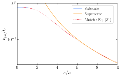
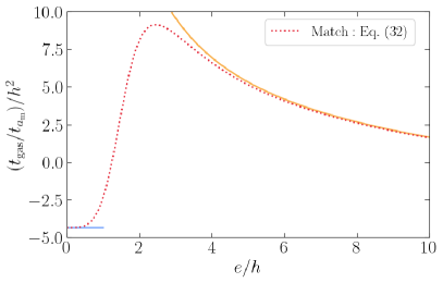
Figure 2: Phenomenological model proposed in Eqs. (31)-(32) for the evolution timescales of the semi-major axis $a_{\text{m}}$ and eccentricity $e$ due to the interaction with the disk, which recovers the analytical estimates presented in Table 1 in their respective limits. This model is based on numerical fits to hydrodynamical simulations Papaloizou and Larwood (2000); Cresswell and Nelson (2008); Ida et al. (2020).

The results from the previous two subsections are summarized in Table 1. When $e\sim h$, the linear analysis from dynamical friction is known to diverge due to the formation of shocks, and non-linear corrections become necessary Muto et al. (2011); Vicente et al. (2019); Suzuguchi et al. (2024); O’Neill et al. (2024). To match the two regimes in this transonic region, we use a phenomenological model based on fits to hydrodynamical simulations Papaloizou and Larwood (2000); Cresswell and Nelson (2008); Ida et al. (2020)

$$\frac{t_{\text{gas}}}{t_{e}} = 0.78\Big{/}\left(1+\frac{1}{30}\left(\frac{e}{h}\right)^{3}\right),$$ (31)

$$\frac{t_{\text{gas}}}{t_{a_{\text{m}}}} = 2C_{\text{Sub}}\,h^{2}\left(1-e^{2}\right)\frac{1-\left(\frac{e}{1.25h}\right)^{4}}{1+\left(\frac{e}{1.75h}\right)^{5}}\,.$$ (32)

This model is illustrated in Fig. 2, compared to the analytical estimates given in Table 2 for subsonic and supersonic limits.

One might question how the results presented in the next sections depend on the matching condition imposed for $e\sim h$, in particular, on the steepness of the transition or the presence of the bump in $1/t_{a_{m}}$ at $e\sim 2h$. We explore this in Appendix A and conclude that our results for the measurement precision of the disk parameters only differ by $\mathcal{O}(1)$, and the overall qualitative picture is left unchanged. We note, however, that the bump in the transition region of $1/t_{a}$ has been reported in several studies and is linked to the resonant excitation of sound waves when the relative velocity of the secondary with respect to the gas flow matches the sound speed, which occurs at $e\sim h$ (in particular see Fig. 1 in Ida et al. (2020)).

Also, recall that we are ignoring relativistic corrections while EMRIs inherently probe strong-field gravity. From previous studies Barausse (2007); Traykova et al. (2023), we expect relativistic corrections in dynamical friction to add a factor of $\sim\left(1+\Delta v^{2}\right)^{2}/\left(1-\Delta v^{2}\right)$ to the overall force. For the eccentricities we are going to consider ($e\lesssim 0.2$), $\Delta v\sim 0.1$, and this is only a factor of $\sim 1-2$ (see Fig. 1 in  Barausse (2007)).

Finally, the extension of Eqs. (31)-(32) to orbits with small inclination, such that the secondary always stays immersed in the accretion disk (i.e., $e\lesssim h$) is straightforward Papaloizou and Larwood (2000); Cresswell and Nelson (2008); Ida et al. (2020). Here, we focus on equatorial motion because inclination is expected to damp more efficiently than eccentricity as a result of the interaction with the disk Wang et al. (2024).

II.3 FastEMRIWaveform package and Fisher-Information Matrix

With a model for the binary-disk interaction in place, we now need a framework for waveform computation and data analysis to study the detectability of gas effects with future EMRI observations.

For the waveform, we use the modular FastEMRIWaveform (few) package Chua et al. (2021); Katz et al. (2021), which allows to input corrections to the trajectory of an EMRI by adding terms to the evolution equations governing the orbital parameters

$$\dot{a}_{\text{m}} = \left(\dot{a}_{\text{m}}\right)_{\text{GW}}+\left(\dot{a}_{\text{m}}\right)_{\text{gas}}\,,$$ (33)

$$\dot{e} = \dot{e}_{\text{GW}}+\dot{e}_{\text{gas}}\,.$$ (34)

Here, the subscript ‘GW’ refers to the contribution from gravitational radiation and ‘gas’ to the interaction with the disk, described in the previous sections. The term $\left(\dot{a}_{\text{m}}\right)_{\text{GW}}$ is the same as in vacuum GR because we neglect the disk’s self-gravity (seen in Ref. Kocsis and Loeb (2008) to be a subdominant effect). The gravitational fluxes are computed based on self-force theory, where Einstein’s equations are solved perturbatively in the mass ratio $\varepsilon$ Barack and Pound (2019); Pound and Wardell (2021). The modified trajectory is then fed into a module to compute the waveform. A key property in this procedure is the fact the orbital phases vary on much shorter timescales than quantities that characterize the orbit, such as the orbital energy and angular momentum Hinderer and Flanagan (2008); Miller and Pound (2021, 2021), allowing to consider orbit-averaged values for $\left(\dot{a}_{\text{m}}\right)_{\text{gas}}$ and $\dot{e}_{\text{gas}}$, capturing their secular evolution. For the systems we will study, typically $\left(\dot{a}_{\text{m}}\right)_{\text{gas}}/\left(\dot{a}_{\text{m}}\right)_{\text{GW}}\lesssim 10^{-3}$ and $\dot{e}_{\text{gas}}/\dot{e}_{\text{GW}}\lesssim 10^{-2}$.

We use a fully relativistic implementation of the Schwarzschild, eccentric waveforms publicly available in few , accurate to leading order in the mass ratio $\varepsilon$ (the adiabatic order). SMBHs are actually expected to have large spin, but a generic, fully-relativistic implementation of Kerr eccentric waveforms is currently being developed. Nonetheless, BH spin should not play a significant role in the measurement of disk effects. This is because spin corrections are more important close to plunge, while environmental effects are more relevant in the early inspiral (they are effectively a negative Post-Newtonian correction, whereas spin corrections enter at 1.5 Post-Newtonian order Poisson and Will (2014)). We could use approximate, non-fully relativistic waveform models (e.g. the Augmented Analytic Kludge model Chua et al. (2017)), which are available for spinning BHs at larger radii, but it was recently noted that these approximants tend to underestimate the power in the early inspiral relative to the plunge Khalvati et al. (2024). Since this is when the interaction with the disk is more important, and the constraints change substantially when using these approximate waveforms, we opt to employ the fully relativistic ones despite their current limitations in the coverage of the parameter space.

For the data analysis, we use the Fisher-Information Matrix Vallisneri (2008) to estimate the statistical uncertainty on a (single) measurement of the true source parameters. In particular, we employ the StableEMRIFisher(SEF) package . The Fisher-Information Matrix is valid in the limit of high signal-to-noise ratio (SNR), assuming a flat prior in the parameter region of interest and stationary, Gaussian noise Vallisneri (2008). Under these assumptions, the posterior distribution of the source parameters $\bm{\theta}$ is given by a multivariate normal distribution around the true values, with covariance $\bm{\Sigma}=\bm{\Gamma}^{-1}$ defined by the inverse of the Fisher matrix

$$\Gamma_{ij}=4\text{Re}\int_{0}^{\infty}\frac{1}{S_{n}(f)}\left(\frac{\partial\tilde{h}^{*}}{\partial\theta_{i}}\right)\left(\frac{\partial\tilde{h}}{\partial\theta_{j}}\right)df\,.$$ (35)

Here, $\tilde{h}=\tilde{h}(f;\bm{\theta})$ is a waveform template in the frequency domain (in our case computed with few) and $S_{n}(f)$ is the one-sided detector’s noise spectral density Babak et al. (2021). More explicitly, the uncertainty in $\theta_{i}$ is given by the $i$th-diagonal element of $\bm{\Sigma}$

$$\Delta\theta_{i}=\sqrt{\Sigma_{ii}}\,.$$ (36)

The covariance matrix also determines the correlations between different parameters

$$\Delta\theta_{i}\Delta\theta_{i}=\Sigma_{ij}\,.$$ (37)

For $S_{n}(f)$, we use the SciRDv1 curve for instrumental noise Team (2018), and include the galactic confusion noise Karnesis et al. (2021) with assumed duration of 4 years.

It will be useful to obtain the Fisher-Information Matrix for a new set of source parameters $\tilde{\bm{\theta}}$ having computed it from the previous set $\bm{\theta}\left(\tilde{\bm{\theta}}\right)$. Having the Jacobian

$$J_{ij}=\frac{\partial\theta_{i}}{\partial\tilde{\theta}_{j}}\Bigg{|}_{\bm{\theta}=\bm{\theta}_{\text{true}}}\,,$$ (38)

one just applies the transformation

$$\tilde{\bm{\Gamma}}\left(\tilde{\bm{\theta}}\right)=\bm{J}^{\text{T}}\cdot\bm{\Gamma}\left(\bm{\theta}\left(\tilde{\bm{\theta}}\right)\right)\cdot\bm{J}\,.$$ (39)

Finally, the FIM also allows to compute the inference bias $\Delta\bm{\theta}$ in the EMRI parameters if the environmental effects are not considered in the analysis. Let us denote the disk-related parameters by $\bm{\theta}_{\text{bv}}$ (beyond-vacuum) and the others by $\bm{\theta}_{\text{v}}$. Additionally, $\bm{\theta}^{0}_{\text{bv}}$ denotes the value of $\bm{\theta}_{\text{bv}}$ for which the environmental effects are zero (e.g. $\Sigma_{0}=0$ and any $h_{0}$). Then Cutler and Vallisneri (2007); Kejriwal et al. (2023)

$$\Delta\bm{\theta}_{\text{v}}=\left[\left(\bm{\Gamma}\right)^{-1}_{\bm{\theta}_{\text{v}}\bm{\theta}_{\text{v}}}\cdot\bm{\Gamma}_{\bm{\theta}_{\text{v}}\bm{\theta}_{\text{bv}}}\right]\Bigg{|}_{\bm{\theta}^{0}_{\text{bv}}}\cdot\left[\bm{\theta}_{\text{bv}}-\bm{\theta}^{0}_{\text{bv}}\right]\,.$$ (40)

III Results

Having developed a model for the effect the disk has on the EMRI evolution, and a framework for the inference of the disk properties with GW observations, we now present the results of our study.

III.1 Constraints on Accretion Physics

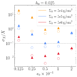
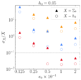
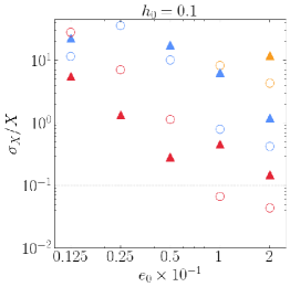
Figure 3: Measurement uncertainty computed via the Fisher-Information Matrix (35) for the disk central surface density, $\Sigma_{0}$, and aspect ratio, $h_{0}$, for an EMRI evolving in different accretion configurations (different pairs $\{\Sigma_{0},h_{0}\}$) as a function of its initial eccentricity $e_{0}$. All other parameters of the EMRI are kept fixed and are listed in Table 2. The initial semi-lactus rectum is chosen so that the EMRI is close to plunge after 4 years of observation with LISA. Larger $\Sigma_{0}$, smaller $h_{0}$ and larger $e_{0}$ help probing accretion physics, in particular if during the evolution the EMRI transitions from supersonic to subsonic motion relative to the gas flow in the disk, which occurs for $e\sim h$. The grey horizontal line, corresponding to $\sigma_{X}/X=0.1$, serves for illustration purposes only. Given a particular disk model, constraints on $\Sigma_{0}$ and $h_{0}$ can be transformed to constraints on the accretion rate and viscosity, which we show in Fig. 4 for the Shakura-Sunayev $\alpha$-disk model.

We focus on a “typical” EMRI, varying only its initial eccentricity while fixing the other parameters. The only exception is luminosity distance, which we vary in order to maintain the same SNR for all eccentricities. The parameters are listed in Table 2, and were picked to be similar to the previous study on circular inspirals Speri et al. (2022a). The initial orbital separation is chosen so that the EMRI is close to plunge after 4 years of observations. Apart from the zero spin (justified in the previous section), the EMRI’s parameters are within the expected values as listed in the LISA Definition Study Report Colpi et al. (2024). The secondary is chosen to be heavy to mimick mass growth via accretion in the disk during EMRI formation Bondi and Hoyle (1944). In fact, LISA could detect even heavier secondaries, in light of recent studies on intermediate-mass black holes Abbott et al. (2020); Rose et al. (2022); Mezcua (2017). This would yield larger SNRs and allows us to probe larger orbital separations, where the environmental effects are stronger, which would in turn improve our projected constraints on the disk parameters.

$M$	$10^{6}\,M_{\odot}$
$\mu$	$50\,M_{\odot}$
$a/M$	0
$p_{0}/M$	16.83
$\Phi_{\varphi 0}$	$\pi/3$
$\Phi_{r0}$	$\pi/2$
$\theta_{S}$	0.9
$\phi_{S}$	1.5
$T_{\text{obs}}$	4 years
SNR	50

Table 2: EMRI parameters fixed to study the variation of the constraints on the accretion disk parameters $\{\Sigma_{0},\,h_{0}\}$ as a function of the initial eccentricity $e_{0}$ of the EMRI (Figs. 3-4 and Section III.1). The parameters are: $M$ - primary mass; $\mu$ - secondary mass; $a$ - primary spin; $p_{0}$ - initial semi-lactus rectum; $\{\Phi_{\varphi 0},\Phi_{r0}\}$ - initial phases of the periodic motion in the azimuthal and radial direction, respectively; $\{\theta_{S}\,,\phi_{S}\}$ - polar and azimuthal sky location angles, respectively; $T_{\text{obs}}$ - observation time with LISA; SNR - signal-to-noise ratio; The luminosity distance is varied for different initial eccentricities to keep the SNR fixed. For the parameters listed the luminosity distance is approximately $d_{L}\sim 4\,\text{Gpc}$.

We pick a set of 5 initial eccentricities – $e_{0}=\{0.0125,\,0.025,\,0.05,\,0.1,\,0.2\}$ – and compute the Fisher-Information Matrix (35) for the EMRI system in Table 2 and $9$ different disk configurations, corresponding to different pairs of the central surface density — $\Sigma_{0}=5\times\{10^{4},\,10^{5},\,10^{6}\}\,\left[\text{g}/\text{cm}^{2}\right]$ — and the central aspect ratio — $h_{0}=\{0.025,\,0.05,\,0.1\}$. As mentioned when the disk model was introduced in Sec. II.2, these are compatible with numerical simulations and observations.

In Fig. 3 we show the relative error computed from the Fisher-Matrix for $\Sigma_{0}$ and $h_{0}$ for all configurations. The statistical errors for the other EMRI parameters are of the same order of magnitude as in vacuum. We thus choose to only show the full corner plots for two configurations in Appendix B, one corresponding to initial subsonic motion and the other to initial supersonic motion.

Larger densities and smaller aspect ratios lead to larger corrections to the inspiral, independently of whether the EMRI is in the subsonic or supersonic regime, and thus these configurations optimize the constraints on the disk parameters. For $h_{0}=0.1$, it is not possible to probe the effect of the accretion disk for any of the eccentricities, since all measurements of the density would be consistent with 0, i.e. no disk, within $1-\sigma$ uncertainty. This is also true for all configurations with $\Sigma_{0}=5\times 10^{4}\,\text{g}/\text{cm}^{2}$. To probe these densities/aspect ratios we would require EMRIs with larger SNR, e.g. closer to Earth, and/or that start from larger orbital separations, e.g. with larger mass ratio.

Nonetheless, there are a couple of configurations for which both $\Sigma_{0}$ and $h_{0}$ would be measurable with a relative error smaller than $10\,\%$, even with $e_{0}$ as small as $0.025$ ($h_{0}=0.025$ in the left panel). We note that this is not possible for circular motion, for which these parameters only enter the correction to the semi-major axis through the ratio $\Sigma_{0}/h_{0}^{2}$, and are therefore completely degenerate. It is also clear that eccentricity plays a major role in ’deviating’ the wet EMRI from a typical vacuum inspiral. In fact, throughout the inspiral the relative difference in the eccentricity evolution between in-disk and in-vacuum is typically one order of magnitude larger than the same relative difference in the semi-lactus rectum evolution.

The initial eccentricity that minimizes the measurement uncertainty varies with $h_{0}$, and is related to whether the EMRI transitions from the super to the subsonic regime during the inspiral. As seen earlier, during this transition the functional dependence on $h_{0}$ on the rate of change of the orbital parameters changes (check Table 1 and Fig. 2). Although this complicates the model, it likely breaks correlations with other parameters. When the initial eccentricity is either substantially smaller or larger than the aspect ratio, the EMRI spends most of its inspiral in, respectively, the subsonic or supersonic regime. This effectively makes the correction to the trajectory due to the environment simpler and, therefore, harder to constrain, as seen in the panel for $h_{0}=0.025$. Also recall that in the transition from super-to-subsonic motion, there is an enhancement in the damping of the orbital separation due to the resonant excitation of sound waves in the gas (the bump at $e\sim 2h$ in the right panel of Fig. 2). In Appendix A, we show results for a smoother profile (see Fig. 5), and conclude the qualitative behavior observed in Fig. 3 is maintained. In fact, a bump less pronounced does not necessarily imply measurements less precise, as illustrated in Fig 6.

Despite the measurement uncertainties being of the same order of magnitude as in vacuum, we observe a change in some correlation signs depending on whether the EMRI starts in subsonic or supersonic motion. For example, in vacuum, there is typically a strong negative correlation between $M-p_{0}$, which is also observed in the fully subsonic case (Fig. 7). Intuitively, as the initial semi-lactus rectum increases, so does the time to plunge, which can be compensated by a decrease in the primary mass. However, as the initial ratio $e_{0}/h_{0}$ increases, indicating the EMRI starts the inspiral in the supersonic regime, the $M-p_{0}$ correlation becomes positive (Fig. 8), which was confirmed for different $h_{0}$. Similar sign changes occur, for example, for $M-e_{0}$ and $p_{0}-\Sigma_{0}$ correlations. We attribute this to the intricate transonic behavior of the inspiral. In fact, if the EMRI’s initial eccentricity is very large (e.g. $e_{0}=0.6$) and it spends the whole observation window in the supersonic regime, we recover the same correlations as in the subsonic case. We note that changes in correlation signs have been observed in other EMRI systems, e.g. eccentric EMRIs with scalar charge Speri et al. (2024), or when trying to recover a vacuum signal with an approximate template Katz et al. (2021). We also confirmed the stability of the Fisher-Matrix in these cases by adopting different parameterizations, in particular by working in $\log M$ and $\log\mu$, and checked the smooth transition in the $M-p_{0}$ correlations as $e_{0}$ increases, by computing more values of $e_{0}$ closer to each other.

Similarly to circular EMRIs Speri et al. (2022a), we found for some disk configurations significant bias in the intrinsic parameters, shifted $3\sigma$ away from their true value, if the effect of the disk is not taken into account in the inference. Conversely, the extrinsic parameters (sky location and luminosity distance) displayed much smaller bias. Yet, we found the Fisher-Matrix was more prone to numerical instabilities when computed at the null hypothesis, i.e. at the values of the disks parameters $\bm{\theta}=\bm{\theta}^{0}_{\text{bv}}$ for which their effect is null, which is necessary for the bias computation according to Eq. (40). We therefore leave for future work a more thorough study of these bias over the parameter space. As shown in Ref. Speri et al. (2022a), the bias can be so significant after 4 years of observation that the signal can be missed within the small prior volume typically used in fully Bayesian inference for EMRI parameter estimation. The signal could still be caught using smaller chunks of data, but one would see the maximum likelihood estimators drifting from the true value as the observation time increases (and SNR not accumulating). This would be a data-driven smoking gun of the presence of a beyond-vacuum effect.

If we specify a particular accretion disk model, we can relate the surface density and aspect ratio with internal disk properties like accretion rate and viscosity, as made explicit in Eqs. (4)-(5) for the Shakura-Sunayev $\alpha$-disk. Then, using Eqs. (38)-(38), we can obtain the Fisher-Information matrix for this new set of parameters and compute their measurement uncertainty. We show this in Fig. 4 for $h_{0}=0.025$. For some systems one can simultaneously constraint the viscosity, $\alpha$, and the accretion rate-efficiency ratio, $f_{\text{Edd}}/\epsilon$. As mentioned before, this is not possible in circular orbits where these parameters become completely degenerate and one can only constrain an overall amplitude in $(\dot{a}_{\text{m}})_{\text{gas}}$ which captures some combination of $\alpha$ and $f_{\text{Edd}}/\epsilon$ (check Eq. (2.2) in Speri et al. (2022a)). To then break this degeneracy, one would need an electromagnetic counterpart to the GW signal to yield an independent measure for the accretion rate.

III.2 Formation Channels

The differences between the supersonic and subsonic interactions also have implications for for the formation of wet EMRIs. As commented in the Introduction, previous studies on these systems argued they should be (quasi)circular Pan et al. (2021); Pan and Yang (2021) because, in the subsonic regime, density waves damp eccentricity on a much faster timescale than migration. One can see this explicitly from the first row in Table 1 where $t_{e}/t_{a_{\text{m}}}\sim h^{2}\ll 1$. However, as seen above, in the supersonic regime, local dynamical friction is the dominant environmental effect and for large eccentricities (with respect to the aspect ratio $h$), migration actually occurs faster than eccentricity damping. From the second row in Table 1, one can see explicitly that $t_{e}/t_{a_{\text{m}}}\sim(e/h)^{2}\gg 1$ for supersonic motion. This behaviour puts into question the expectation that wet EMRIs will be circular. There are also other environmental interactions which excite eccentricity, such as stochastic fluctuations in the gas flow Nelson (2005); Johnson et al. (2006), retrograde orbits Sánchez-Salcedo et al. (2018); Sánchez-Salcedo (2020), or dynamical friction in dark matter distributions Cardoso et al. (2021b); Tomaselli et al. (2024).

Recently, Ref. Wang et al. (2024) considered the impact of some of these effects in the formation of stellar-origin BH binaries in AGN disks, concluding that for initial retrograde orbits ‘there might be some eccentricity residual on captured BHs’. It is clear from the examples above that the assumption of quasi-circularity for EMRIs forming in accretion disks needs to be reconsidered. We leave for future work a quantitative study of the effect that stochasticity and interaction with a DM distribution have on the eccentricity distribution of a population of wet EMRIs. We also note that equal mass binaries surrounded by circumbinary disks have been recently found to evolve to fixed points in eccentricity Ishibashi and Gröbner (2024); Franchini et al. (2024) (see also Refs. Tomaselli et al. (2024) for a similar behavior in ultralight dark matter environments).

Reference Wang et al. (2024) also found inclination is always zero (for the purposes of LISA precision) by the time the EMRI is captured and eventually enters the LISA band, independently of its initial conditions. Nonetheless, inclined orbits are relevant in the context of periodic electromagnetic signals associated to EMRIs at large radial separations, which we discuss in more detail in the next subsection.

III.3 Host identification and multimessenger EMRIs

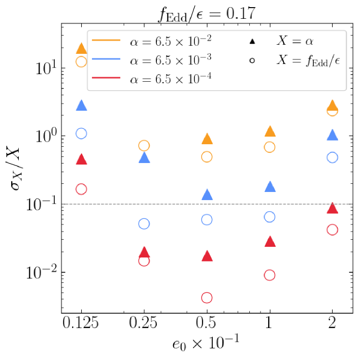
Figure 4: Same as in the left panel of Fig. 3 ($h_{0}=0.025$), but transforming constraints in the surface density and aspect ratio $\{\Sigma_{0},\,h_{0}\}$ into constraints on the accretion rate and viscosity $\{f_{\text{Edd}}/\epsilon,\,\alpha\}$ for the Shakura-Sunayev model (4)-(5).

We now discuss the possibility of detecting an electromagnetic (EM) counterpart to eccentric wet EMRIs, making these sources candidates for standard sirens. This can be accomplished by identifying the host galactic nucleus, and/or by observing an EM counterpart directly linked to the EMRI’s orbital motion.

Let us start with the identification of the host galaxy. By the time LISA flies, the Vera C. Rubin Observatory Legacy Survey of Space and Time (LSST) will have provided the most complete AGN catalog, down to the luminosities of Seyfert galaxies and up to high redshift, and covering $18000\,{\rm deg}^{2}$ – almost half of the sky LSST Science Collaboration (2009). The LSST catalog will have redshift errors of order $\Delta z\sim\pm 0.05$ at low redshifts LSST Science Collaboration (2009), which are sufficiently small compared to the ones obtained for EMRI events, $\Delta z\sim\pm 0.06$ (assuming some cosmology).

Suppose we then detect an EMRI with significant evidence for an environmental effect described by the model we studied. From the GW signal we will measure, with high precision for astrophysical purposes, the SMBH mass and spin, and also the ratio $f_{\text{Edd}}/\epsilon$ (Fig. 4). From the spin, we can estimate the mass-radiation conversion efficiency $\epsilon$ Madau et al. (2014); Mangiagli et al. (2022), from which we can then infer the luminosity Eddington ratio $f_{\text{Edd}}$. With the latter we compute the bolometric luminosity of the AGN hosting the EMRI through $\dot{L}=f_{\text{Edd}}L_{\text{Edd}}$, where $L_{\text{Edd}}=1.26\times 10^{38}\left(M/M_{\odot}\right)\,\text{erg/s}=3.2\times 10^{4}\left(M/M_{\odot}\right)L_{\odot}$, with $L_{\odot}=3.846\times 10^{33}\,\text{erg/s}$ being the Sun’s luminosity. The GW signal also gives a precise measurement of the luminosity distance $d_{L}$. By combining $\dot{L}$ and $d_{L}$, we can infer the apparent magnitude of the AGN in the optical band of the Rubin observatory through Mangiagli et al. (2022)

$$m_{\text{AGN, Rubin}}=M_{\text{AGN, Rubin}}+5\,\log_{10}\left(\frac{d_{L}}{\text{pc}}\right)-5\,,$$ (41)

where $M_{\text{AGN Rubin}}$ is the absolute magnitude (independent of distance) in that instrument’s band Mangiagli et al. (2022)

$$M_{\text{AGN, Rubin}}=4.64-2.5\log_{10}\left(\frac{0.1L}{{L_{\odot}}}\right)\,.$$ (42)

The Rubin Observatory will be sensitive to $m_{\text{AGN, Rubin}}\lesssim 27.5$ (see Section IV in Ref. Mangiagli et al. (2022) for generic expressions for other frequencies/instruments).

Assuming a fiducial value of $\epsilon=0.1$, for the systems studied in Section III.1, only disk configurations with $h_{0}=0.1$ ($f_{\text{Edd}}/\epsilon=0.068$ for the $\alpha$-disk) would yield an apparent magnitude $m_{\text{AGN, Rubin}}=26.8$, smaller than the Rubin threshold. However, for the same EMRI at half the luminosity distance ($d_{L}\sim 2\,\text{Gpc}$), all disk configurations would have detectable magnitudes in the catalog. Higher primary masses and conversion efficiencies, which can go up to $\epsilon\sim 0.4$ for maximally rotating BHs, would also decrease the AGN’s magnitude Madau et al. (2014); Mangiagli et al. (2022). Taking the measurement uncertainties for this brighter sources to be similar to the ones obtained in Sec. III.1 for the most constrained systems ($\Delta f_{\text{Edd}}/f_{\text{Edd}}\sim 0.1$), we find that the GW signal alone gives an estimate of the magnitude with relative error $\Delta m_{\text{AGN, Rubin}}/m_{\text{AGN, Rubin}}\sim 0.01$, whereas the photometric errors by Vera Rubin are $0.005-0.02$, depending on brightness. We could then compare within the EMRI’s sky location error ($\Delta\Omega\sim 2-18\,\text{deg}^{2}$ Colpi et al. (2024)), how many AGNs in the LSST have magnitudes matching the GW estimate. Even if multiple AGNs were compatible, one could do more targeted searches in the sky area identified by the GW measurement, either with Vera Rubin, or with instruments like the Square Kilometer Array (radio) Dewdney et al. (2009), or ATHENA (X-Ray band) 201 (2013). Having a reduced number of possible host galaxies for the EMRI could also improve their use as dark sirens Laghi et al. (2021).

X-Ray observations appear of particular relevance to EMRIs in light of the dozen of recently observed Quasi-Periodic Eruptions/Oscillations (QPE/O) Kejriwal et al. (2024); Linial and Metzger (2023); Franchini et al. (2023); Arcodia et al. (2024); Pasham et al. (2024). These are periodic soft X-Ray signals ($\sim 0.1\,\text{keV}$) thought to originate from a compact object passing twice per orbit through an accretion disk around a SMBH. The orbit is necessarily inclined and several models have been proposed, involving, e.g., the tidal disruption of a main-sequence star Linial and Metzger (2023), or disk precession. The secondary-disk interaction affects the binary’s dynamics, which can be tracked by the periodic variability of the X-Ray emission peaks.

Many QPE/Os were found in galaxies with a SMBH with $\sim 10^{6}\,M_{\odot}$ King (2023), precisely in the mass range interesting for LISA EMRIs. However, their frequencies are typically $\lesssim 10^{-4}\,\text{Hz}$, outside of the LISA band, indicating that the secondaries are currently at large orbital separation, where their evolution could be driven by disk collisions instead of GW radiation reaction. In the future, we might detect a QPE/O in the EM which would enter the LISA band in a decade and be detected through GWs (this was explored in Ref. Kejriwal et al. (2024) for a particular QPO Jin et al. (2020)). As EM observatories improve, we also do not exclude the possibility of observing QPE/Os closer to the central SMBH and directly search for a X-Ray variability in the EMRI’s sky location after its detection. Yet, to better understand the time evolution of the EMRI’s orbit and its corresponding EM counterpart, it is crucial to study the transition from out-of-equatorial plane to in-plane motion, where the secondary becomes fully immersed in the disk and could follow an evolution similar to the model we studied. We expect significant developments in this problem as more data is collected until LISA launches.

IV Conclusions & Discussion

In this work, we developed a model for the evolution of eccentric EMRIs in accretion disks valid up to eccentricities $e\sim 0.6$. Our model connects analytic results from Newtonian analysis when the small compact object is moving subsonically or supersonically with respect to the gas flow of the disk. While in the subsonic limit the EMRI excites spiral density waves that resonantly exchange angular momentum with the binary throughout the whole disk (migration), in the supersonic case the dominant contribution comes from the local density wake that trails behind the secondary (dynamical friction). These two regimes are “glued” together with hydrodynamical simulations capturing the transition between then.

Using our model, we showed that eccentricities as small as $e\sim 0.025$ when the binary enters the LISA band can significantly improve the measurement of the environmental effects caused by the binary-disk interaction and consequently the inference of the disk properties, like its density/height or viscosity/accretion rate. Their simultaneous constraint is not possible for circular orbits, where they become fully degenerate, and for which EM identification is needed to measure for both viscosity and accretion rate. The fact that for eccentric wet EMRIs we can obtain an estimate for the primary’s mass accretion rate solely from the GW signal offers the possibility of identifying the host galaxy of the system in an AGN catalog, like the LSST survey by the Vera C. Rubin Observatory. Direct EM counterparts to the GW event could also be observed with targeted searches on luminosity periodic variability consistent with the EMRI’s orbital period, like the recently detected Quasi-Periodic Eruptions/Oscillations.

Despite our simplistic model, drawn mostly from works on (Newtonian) planetary migration, and the limited region of the parameter space we explored, our results highlight the importance of more detailed modelling of beyond-vacuum GR effects in binary coalescence for future GW astronomy. Just a simple refinement from previous studies of EMRIs in accretion flows – the inclusion of eccentricity – leads to more interesting phenomenology which can act as distinctive smoking-guns for these astrophysical environments, enhancing their detectability. This is particularly relevant considering the multiple degeneracies in EMRI parameter space Chua and Cutler (2022). These can potentially hinder constraints for beyond-vacuum GR corrections, especially when multiple ones are included simultaneously in the analysis of the GW signal Kejriwal et al. (2023). As better models are developed, we will also be able to assess their relevance when compared to the precision of future GW detectors, i.e. how large the systematics in the modelling of the environmental effects are compared to the statistical uncertainty in their measurement.

Our study should by no means be taken as a final answer to this problem, but rather as yet another example of the rich physics associated to environmental effects in the formation and evolution of compact binaries. We stress that there is room for improvement in our model, by considering more sophisticated disk strucutures (e.g. numerical profiles), stochastic oscillations in the gas flow, inclined orbits, mass accretion onto the secondary and relativistic corrections. An important follow-up would be to compare our results for eccentric inspirals with state-of-the-art hydro codes capable of evolving I/EMRIs immersed in accretion disks. This comparison has been done only for circular orbits Derdzinski et al. (2021), where it was found that for sufficiently light secondaries and “warm” disks (large viscosities), the overall effect in the binary is well captured by the analytic migration formula, up to some numerical factor of $\mathcal{O}(1)$. However, when the disk relaxation timescale is comparable to the binary’s inspiral timescale, which occurs for heavier secondaries and colder disks (smaller viscosities), the binary-disk interaction becomes chaotic and the forces felt by the secondary exhibit strong fluctuations, differing from the analytic result. In this limit, the orbital evolution is no longer adiabatic, i.e. we can no longer consider orbit-averaged effects. In fact, this brings us to the more generic problem of how to accurately include environmental effects in the framework of self-force theory, which relies on the two-timescale expansion to separate the orbital timescale, $T_{\text{o}}\sim M$, from the inspiral timescale, $T_{\text{i}}\sim M^{2}/\mu$, where quantities that characterize the orbit vary (e.g. energy, angular momentum).

Our analysis of measurability of these effects with LISA was also simplistic. Complementing the Fisher-Matrix with fully Bayesian inference using e.g. Markov Chain Monte Carlo methods would be valuable, but even more relevant than that would be understanding how to search for deviations from vacuum in the context of the LISA Global Fit Littenberg and Cornish (2023); Katz et al. (2024); Strub et al. (2024). LISA will observe $\sim 10^{4}$ different signals – corresponding to galactic binaries, EMRIs, massive binaries, stochastic GW backgrounds – which need to be searched and analysed simultaneously Speri et al. (2022b). One of the hardest challenges of this scheme are precisely EMRIs, which even in vacuum exhibit a very degenerate parameter space, with numerous secondary modes Chua and Cutler (2022). We are then faced with the question of how to include beyond-vacuum-GR effects on top of the vacuum problem. Doing it directly in the Global Fit pipeline could become too technically demanding and computationally expensive. However, considering these effects are typically small corrections (as it is the case here), we can envision a scenario where we use the residuals obtained from the vacuum-only Global Fit to reanalyse a single source (e.g. the EMRI with largest SNR), to search for additional physics, like the disk interaction considered in this work. We plan to address some of the problems listed above in the near future.

Appendix A Different Migration Models

In this Appendix, we explore the impact in our results from imposing a different matching condition between supersonic and subsonic motion for the evolution of the orbital parameters. In particular, we prescribe a milder transition for the semi-major axis, removing the bump present at $e\sim 2h$ in $t_{\text{gas}}/t_{a}$ (32) (right panel of Fig. 2). We repeat, however, that an enhancement of the disk interaction is expected near the transonic region due to formation of shock waves. Nonetheless, considering astrophysical uncertainties and discrepancies between different hydrodynamical codes, we seek to evaluate how significant the increase in $(\dot{a}_{\text{m}})_{\text{gas}}$ is to the constraints obtained for the disk properties (Sec. III.1 and specifically Fig. 3). We propose a different phenomenological model given by

$$\frac{t_{\text{gas}}}{t_{a_{\text{m}}}}=2C_{\text{sub}}\,h^{2}\left(1-e^{2}\right)\frac{1-\left(\frac{e}{2h}\right)^{2}}{1+\left(\frac{e}{3h}\right)^{3}}\,.$$ (43)

The comparison between this and the model used in Eq. (32) is illustrated in Fig. 5.

Figure 5: Comparison between two phenomenological models for the evolution timescale of the semi-major maxis $a_{\text{m}}$ due to the interaction with the gas disk. One contains a bump near the transonic region ($e\sim 2h$) due to the resonant excitation of sound waves and corresponds to Eq. (32), used for the study in the main text of this work. The other has a “milder” transition between the supersonic and subsonic motion and corresponds to Eq. (43).

We repeat the study done in Section III.1 using the “milder” model, for the same EMRI system (full parameters listed in Table 2) and the different disk configurations. Our results for the measurement uncertainty for the central surface density and aspect ratio of the disk as a function of the initial eccentricity are shown in Fig. 6 for $h_{0}=0.025$ (left panel of Fig. 3). We also plot in faded colours the constraints obtained with the main model to facilitate comparison between the two.

For most of the parameter space, the model without the enhancement in the transonic region leads to less tight constraints, which is intuitive considering the relative amplitude of the gas effect in the evolution of the orbital separation with respect to the GW radiation reaction is smaller. Nonetheless, the difference in the measurement uncertainty ($\sigma_{X}/X$) is almost always a factor of $\mathcal{O}(1)$. We also note that for some disk configurations the constraints obtained with the model without the bump (43) are better, highlighting the need for more detailed modelling of disk interactions in EMRI evolutions.

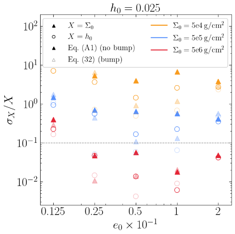
Figure 6: Same as in the left panel of Fig. 3, but for the “milder” model for the correction to the evolution of the semi-major axis $(a_{\text{m}})_{\text{gas}}$ presented in this Appendix, corresponding to Eq. (43) and illustrated in Fig. 5. We also plot in faded colour the results shown in the left panel of Fig. 3 to facilitate comparison between the two models.

Appendix B Full corner

In this Appendix, we show two examples of the full corner plot computed via the Fisher Information Matrix for the same EMRI system (Table 2) and disk configuration ($\Sigma_{0}=5\times 10^{5}\,\text{g}/\text{cm}^{2}$, $h_{0}=0.025$) and two different initial eccentricities. One corresponds to a fully subsonic inspiral ($e_{0}=0.0125$ in Fig. 7) and another to an EMRI that starts in the supersonic regime and transitions to subsonic during the inspiral ($e_{0}=0.05$ in Fig. 8)

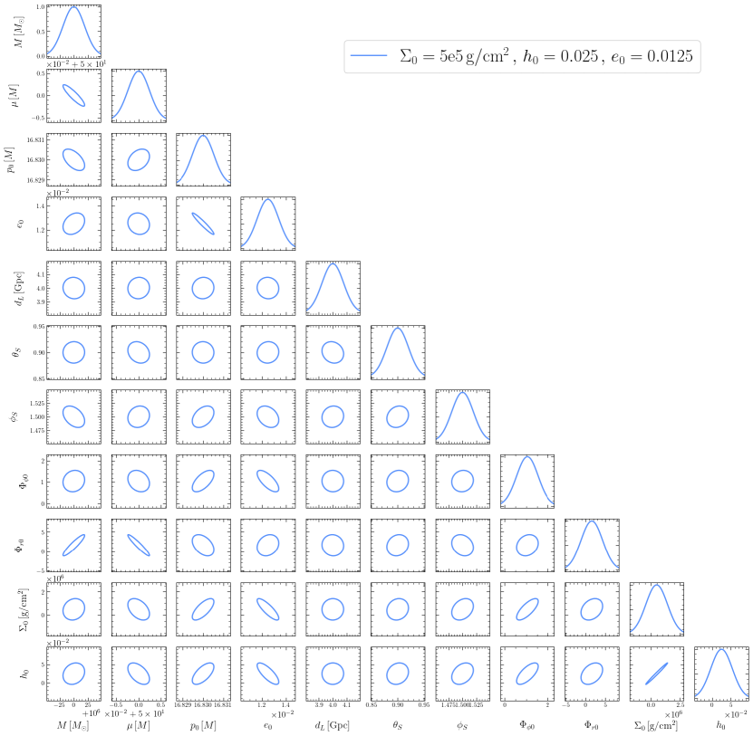
Figure 7: Full corner plot computed via the Fisher-Information Matrix for the EMRI system in Table 2, with initial eccentricity $e_{0}=0.0125$ and disk configuration $\Sigma_{0}=5\times 10^{5}\,\text{g}/\text{cm}^{2}$ and $h_{0}=0.025$. The EMRI is always in the subsonic regime and its eccentricity after 4 years of inspiral is $e_{f}=3.3\times 10^{-3}$.

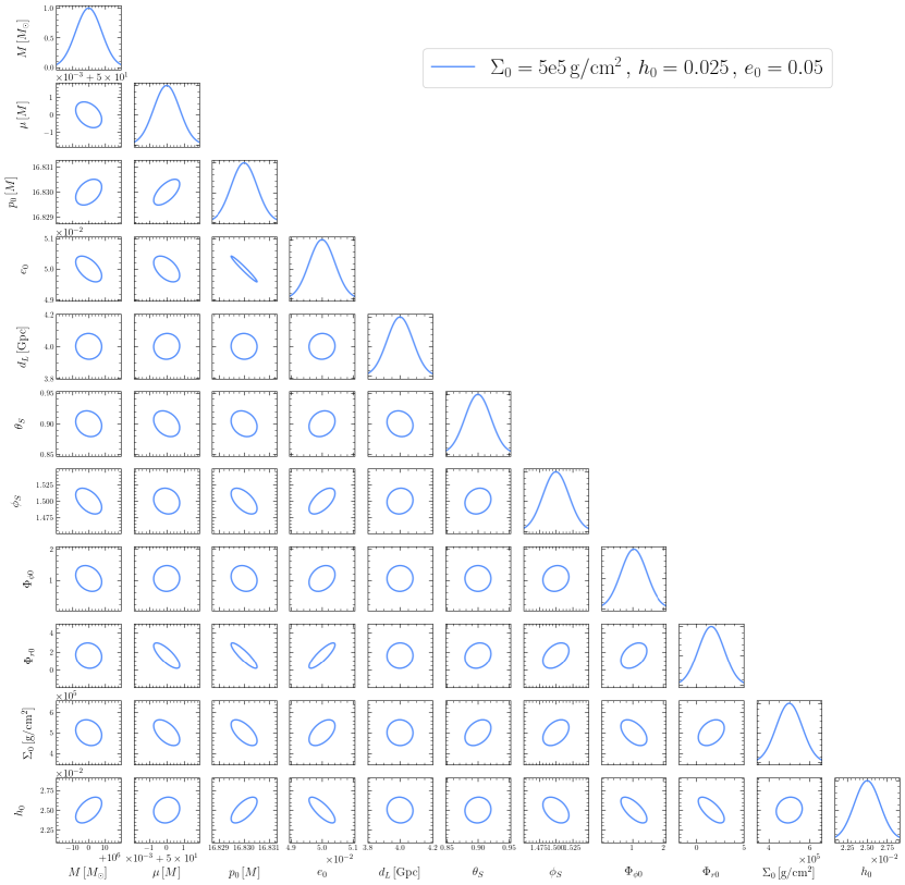
Figure 8: Same as in Fig. 7 for initial eccentricity $e_{0}=0.05$. The EMRI starts in supersonic motion and transitions to subsonic one during the inspiral, having $e_{f}=1.3\times 10^{-2}$ after 4 years of evolution. Notice that the $M-p_{0}$, $M-e_{0}$, $p_{0}-\Sigma_{0}$ correlations change sign with respect to the fully subsonic case.