Mapping the Phase Diagram of a Frustrated Magnet:
Degeneracies, Flat Bands, and Canting Cycles on the Pyrochlore Lattice

Abstract

We map the complete classical phase diagram of the spin Hamiltonian describing pyrochlore rare-earth magnets with all symmetry-allowed nearest-neighbor bond-dependent anisotropic two-spin interactions. We provide a simple derivation of the organization of spins into tensor degrees of freedom describing the multipole moments of a tetrahedron, whose components correspond to irreducible representations (irreps) of the tetrahedral symmetry group $T_{d}$. By parameterizing the Hamiltonian directly in terms of the energies of the individual irreps, we perform an exhaustive search of all possible irrep degeneracies which may host stable classical spin liquids. Doing so reveals four one-parameter families of models along which three phases are degenerate, all four of which merge at the Heisenberg antiferromagnet and its dual, and we give a complete three-dimensional picture of the phase diagram showing all of the phases and their intersections. The appearance of two copies of a single irrep implies an extra degenerate locus which pierces the phase boundaries at special points, yielding two additional isolated triple points. We demonstrate that one-parameter families of Hamiltonians are characterized by a topological invariant describing how the ground state spin configuration winds when adiabatically transported around this degenerate locus, analogous to a “diabolical locus”. We provide a comprehensive catalog of all flat band degeneracies in the phase diagram and discuss the mechanisms that may allow for or impede the realization of a variety of classical spin liquids described by tensor gauge fields exhibiting pinch line singularities and concomitant four-fold pinch points. Lastly, we provide a list of all cases where three irreps are degenerate above the ground state, which may lead to interesting features in the spin wave spectrum within each ordered phase.

I Introduction

The experimental search for, and theoretical classification of, exotic states of matter such as topological phases and deconfined critical transitions, along with their associated spectra of fractionalized excitation, is a central aim of modern condensed matter physics. A core focus is to understand systems whose low-energy physics is not characterized by conventional symmetry breaking with a “rigid” order parameter, but instead exhibits emergent liquid-like characteristics due to strong correlations. A central theme in this effort is that novel physics emerges when multiple conventional ordering channels compete with each other, becoming “intertwined” and resulting in physics that is more than the sum of individual parts [1, 2, 3, 4, 5, 6, 7, 8, 9]. One class of systems that have made significant advancements through constant exchange between the experimental and theoretical fronts are frustrated magnets [10, 11]—specifically, magnetic insulators with antiferromagnetic spin interactions frustrated by triangular motifs, such as occurs on the triangular, kagome, and pyrochlore lattices. The geometric origin of the frustration makes such lattices highly favorable for supporting spin liquids—strongly correlated paramagnetic states which exhibit emergent deconfined gauge fields [12, 13, 14, 15, 16, 17, 18].

In three spatial dimensions the pyrochlore lattice is the premier platform for frustrated magnetism, with multiple families of compounds for experimental study [19, 20, 21, 22, 23, 24] and a solid theoretical understanding of the microscopic physics [25]. It hosts two of the most well-known and canonical examples of spin liquids: the pyrochlore Heisenberg anti-ferromagnet (HAFM) [26, 27, 28] and the pyrochlore Ising anti-ferromagnet, more commonly known as spin ice [29]. Both of these are known to be classical spin liquids, which in the former case refers to the large-spin limit and in the latter refers to the limit where transverse spin-flipping terms are not included in the Hamiltonian. These two models correspond to two distinct limiting cases of the symmetry-allowed spin Hamiltonian: completely isotropic interactions versus the maximally anisotropic limit where spins are constrained to point along their local high-symmetry easy-axes.

Over time the broader problem of considering all symmetry-allowed, bond-dependent, anisotropic spin interactions has become necessary as a plethora of pyrochlore materials have been synthesized and intensively studied [20]. Spatial anisotropies are generically present in these magnets because the “spins” are actually crystal field doublets of $4f$ rare earth ions [36], for which strong spin-orbit coupling makes the interactions sensitive to the local crystalline symmetries [25]. Such bond-dependent anisotropies intermediate between the isotropic and easy-axis limits result in new types of frustration which can yield interesting novel spin liquids [37, 38, 39], most famously in the exactly solved Kitaev Honeycomb model [40, 41, 42]. Indeed, within the phase diagram of the microscopic pyrochlore pseudo-spin-1/2 Hamiltonian with four symmetry-allowed nearest-neighbor spin couplings, a number of classical spin liquids beyond the HAFM and spin ice models have been discovered [43, 44, 45, 46, 47], including some exhibiting emergent tensor gauge fields [45, 46, 47].

Despite many studies, however, a comprehensive picture of the entire phase diagram and how the various models studied fit together has not yet appeared. Given the maturity of research on pyrochlore magnetism, recent advances in the understanding of classical spin liquids [48, 49, 50, 51], along with many new avenues for experimental research [23, 24, 52], it is warranted to give a complete account of the phase diagram and the various places in it where spin liquidity exists or may be present, how the variety of known examples fit together, and how the tensorial nature of these spin liquids arises. Whereas previous studies have looked at either two-dimensional cross sections of the phase diagram [53, 54, 55, 25, 56] or certain 1-parameter models [43, 57, 46], it is highly desirable to have a complete picture that plainly visualizes how such cuts of the phase diagram fit together, along with how the variety of spin liquids coincide with special degeneracies of the phase diagram. Additionally, recent work in the study of so-called [58] and “unnecessary criticality” [59, 60, 61, 62] have emphasized that phase diagrams may contain non-trivial structures other than phase boundaries, and it would be interesting to know whether such structures exist in the pyrochlore phase diagram. These are the tasks we take up in this paper.

A summary of the layout and core results are as follows. In Section II we introduce the Hamiltonian and its various parameterizations, where Fig. 1 illustrates the bond-dependent nature of the anisotropic interactions. We then provide a novel account of the theoretical basis for the tensorial nature of pyrochlore spin liquids by deriving the tensor multipole decomposition of a single tetrahedron (Table 1) and exposing how it corresponds to an analysis of the irreducible representations (irreps) of the tetrahedral symmetry group, where each of the four distinct irreps corresponds to one ground state phase illustrated in Fig. 2. We pay particular attention to the “canting” of spins due to the continuous mixing of two copies of a single irrep appearing in the symmetry decomposition, illustrated in Fig. 3. In Section IV we then take up the issue of parameterizing the Hamiltonian in a way that can be used to expose all of the possible ground state degeneracies, which we accomplish by parameterizing in a way that allows the irrep energies to be tuned independently. This allows us to give the complete classification of triply-degenerate ground states in Table 3: there are exactly four lines in the phase diagram along which three phases meet, and all four of these lines merge together at the HAFM point where all four phases become degenerate. There is duality related to switching the sign of one of the Hamiltonian parameters, denoted $J_{z\pm}$, so we first map the phase diagram in the $J_{z\pm}=0$ subspace via stereographic projection in Fig. 5, before mapping the full phase diagram in Footnote 13, which shows all of the phases, phase boundaries, and triple lines, which merge at the HAFM point and its dual. In the process we uncover a locus along which the two copies of the repeated irrep are degenerate, and in Section V we show that this special locus defines a topological invariant for 1-parameter families of models which encircle it. Finally, in Section VI we give a full catalog of all degenerate combinations which yield flat band degeneracies in Tables 6, 6 and 6, along with the spin structure factors computed in the self-consistent Gaussian approximation in Figs. 9 and 10, and discuss the connection between pinch lines and fourfold pinch points in tensor spin liquids, illustrated in Fig. 12. We end in Section VII with a discussion of all triple degeneracies that occur in excited states, shown in Fig. 13, which give the phase diagram some further interesting structure and may have interesting imprints on the excitations above the ground state within each phase.

II Symmetry Classification of Ground States

We consider the most general nearest-neighbor spin model on the pyrochlore lattice,

$$H=\frac{1}{2}\sum_{i,j}\sum_{\alpha,\beta=1}^{3}S_{i}^{\alpha}\mathcal{J}_{ij}^{\alpha\beta}S_{j}^{\beta},$$ (2)

where the first sum is over sites $i$ and $j$ of the pyrochlore lattice and $\alpha,\beta$ index the three components of a spin. The matrix $\mathcal{J}$ contains all symmetry-allowed nearest-neighbor spin-spin interactions, and we refer to it as the interaction matrix, restricting to only nearest-neighbor interactions. In this work we treat the spins in the classical large-spin limit as fixed-length vectors, with spin length normalized to unity.

II.1 Hamiltonian and Parameterization of Anisotropic Interactions

The Hamiltonian parameters can be expressed either in a global or a local basis, each of which can be useful to identify special parameter points [55, 25]. If we take $\alpha,\beta$ to refer to the global frame Cartesian components of a spin, with $x$, $y$, and $z$ axes along the cubic symmetry axes, then for two spins in the $x,y$ plane the interaction matrix has four independent components

$$\mathcal{J}_{ij}^{\alpha\beta}=\begin{pmatrix}[c]J_{1}&J_{3}&-J_{4}\\ J_{3}&J_{1}&-J_{4}\\ J_{4}&J_{4}&J_{2}\end{pmatrix}.$$ (3)

This form can be deduced by symmetry by considering all symmetry operations which swap these two spins, which transform as pseduovectors under rotations (discussed further in Section II.3), and demanding that $\sum_{\alpha\beta}S_{i}^{\alpha}\mathcal{J}_{ij}^{\alpha\beta}S_{j}^{\beta}$ be invariant. Since every nearest-neighbor bond is symmetry-equivalent, there are four free parameters in the Hamiltonian.

These symmetry-allowed interactions can equivalently be parameterized in a coordinate-free notation as

$$H=\sum_{\langle ij\rangle} \Big{[}J_{\text{Heis}}\bm{S}_{i}\cdot\bm{S}_{j}+J_{\text{PD}}\bm{S}_{i}[\hat{\bm{r}}_{ij}\hat{\bm{r}}_{ij}^{T}]\bm{S}_{j}+J_{\text{K}}\bm{S}_{i}[\hat{\bm{n}}_{ij}\hat{\bm{n}}_{ij}^{T}]\bm{S}_{j}$$

$$+J_{\text{DM}}\bm{D}_{ij}\cdot(\bm{S}_{i}\times\bm{S}_{j})\Big{]}+\frac{J_{\text{SIA}}}{2}\sum_{i}|\bm{S}_{i}\cdot\hat{\bm{z}}_{i}|^{2},$$ (4)

where $T$ denotes transpose, and we refer to the four interactions as: isotropic Heisenberg (Heis), pseduo-dipolar (PD), Kitaev-like (K), Dzyaloshinskii-Moriya (DM), and a single-ion anisotropy (SIA). The geometric picture of these interactions is illustrated in Fig. 1, which shows a single tetrahedron of the pyrochlore lattice inscribed in a cube: $\smash{\cramped{\hat{\bm{r}}_{ij}\propto\bm{r}_{j}-\bm{r}_{i}}}$ point from site $i$ to site $j$ (gray arrows), where $\bm{r}_{i}$ is the position of site $i$; $\hat{\bm{n}}_{ij}$ are the normal vectors to the cube faces (orange arrows); and $\smash{\cramped{\hat{\bm{D}}_{ij}=\hat{\bm{n}}_{ij}\times\hat{\bm{r}}_{ij}}}$ are the DM vectors. We call the third term Kitaev-like because it involves only $x$, $y$, or $z$ spin interactions on each edge—a $z$-$z$ interaction if $\bm{r}_{ij}$ is in the $x,y$ plane and the others by cyclic permutation. The pseudo-dipolar term is so called because it it appears when truncating a dipole-dipole interaction at nearest-neighbor. In the single-ion anisotropy, $\hat{\bm{z}}_{i}$ is the local easy-axis direction. While single-ion anisotropy is irrelevant for spin-1/2 operators, it will be important for us to include since it is a symmetry-allowed interaction and is required to match the number of parameters in the Hamiltonian with the number of irreducible representations of the point symmetry group.

\begin{overpic}[width=346.89731pt]{DM_vectors.pdf} \put(52.0,48.0){\large$\hat{\bm{r}}_{ij}$} \put(39.0,83.0){\large$\hat{\bm{n}}_{ij}$} \put(18.0,55.0){\large$\hat{\bm{D}}_{ij}$} \put(69.0,82.0){\large$\hat{\bm{z}}_{i}$} \end{overpic}

Figure 1: An illustration of a single tetrahedron inscribed in a cube and the bond-dependent anisotropy vectors which appear in the symmetry-allowed spin-spin interactions in Eq. 4. The local three-fold easy-axis $\hat{\bm{z}}_{i}$ at each corner of the tetrahedron is indicated by a red arrow. The nearest-neighbor separation vector $\hat{\bm{r}}_{ij}$ (gray arrows) point along the edges of the tetrahedron. The normal vectors $\hat{\bm{n}}_{ij}$ (orange arrows) point out of the cube at the midpoint of each tetrahedron edge. The DM vectors $\smash{\hat{\bm{D}}_{ij}}$ (light blue arrows) then lie in the cube faces pointing along the face diagonals orthogonal to the edges of the tetrahedron (thin black lines). Since $\smash{\cramped{\hat{\bm{r}}_{ij}=-\hat{\bm{r}}_{ji}}}$, $\smash{\cramped{\hat{\bm{D}}_{ij}=-\hat{\bm{D}}_{ji}}}$; here we have made a particular choice of $\hat{\bm{r}}_{ij}$. The total interaction $\smash{\cramped{\hat{\bm{D}}_{ij}\cdot\bm{S}_{i}\times\bm{S}_{j}}}$ does not depend on the order of $i,j$.

In addition to the global frame, one can utilize a local symmetry-adapted basis, with a separate frame defined for each spin. The traditional definitions take the local $\hat{\bm{z}}_{i}$ along the 3-fold easy axis, $\hat{\bm{y}}_{i}$ along a 2-fold axis, and $\hat{\bm{x}}_{i}=\hat{\bm{y}}_{i}\times\hat{\bm{z}}_{i}$ lying in a mirror plane. An explicit choice of local coordinates is given in Appendix A. In terms of the local frame $S_{i}^{x}$, $S_{i}^{y}$, and $S_{i}^{z}$ components, defining $S_{i}^{\pm}=S_{i}^{x}\pm iS_{i}^{y}$, the Hamiltonian is given by

$$H =\frac{J_{\text{SIA}}}{2}\sum_{i}(S_{i}^{z})^{2}+\sum_{\langle ij\rangle}\Big{[}J_{zz}S_{i}^{z}S_{j}^{z}-J_{\pm}(S_{i}^{+}S_{j}^{-}+S_{i}^{-}S_{j}^{+})$$

$$+J_{\pm\pm}\gamma_{ij}(S_{i}^{+}S_{j}^{+}+S_{i}^{-}S_{j}^{-})+J_{z\pm}\left(\zeta_{ij}(S_{i}^{+}S_{j}^{z}+S_{i}^{z}S_{j}^{+})+\text{h.c.}\right)\Big{]},$$ (5)

where $\gamma_{ij}$ are cube roots of unity and $\zeta_{ij}=-\gamma_{ij}^{*}$. The global and local parameterizations correspond to a change of basis for $\mathcal{J}$, and are related by a linear map

$$\begin{pmatrix}[l]J_{zz}\\[4.30554pt] J_{\pm\pm}\\[4.30554pt] J_{z\pm}\\[4.30554pt] J_{\pm}\end{pmatrix}=\begin{pmatrix}[r]-\frac{2}{3}&\frac{1}{3}&-\frac{2}{3}&-\frac{4}{3}\\[4.30554pt] \frac{1}{6}&\frac{1}{6}&-\frac{1}{3}&\frac{1}{3}\\[4.30554pt] \frac{1}{3\sqrt{2}}&\frac{1}{3\sqrt{2}}&\frac{1}{3\sqrt{2}}&-\frac{1}{3\sqrt{2}}\\[4.30554pt] \frac{1}{3}&-\frac{1}{6}&-\frac{1}{6}&-\frac{1}{3}\end{pmatrix}\begin{pmatrix}[l]J_{1}\\[4.30554pt] J_{2}\\[4.30554pt] J_{3}\\[4.30554pt] J_{4}\end{pmatrix},$$ (7)

with inverse map

$$\begin{pmatrix}[l]J_{1}\\[4.30554pt] J_{2}\\[4.30554pt] J_{3}\\[4.30554pt] J_{4}\end{pmatrix}=\begin{pmatrix}[r]-\frac{1}{3}&\frac{2}{3}&\frac{2\sqrt{2}}{3}&\frac{4}{3}\\ \frac{1}{3}&\frac{4}{3}&\frac{4\sqrt{2}}{3}&-\frac{4}{3}\\ -\frac{1}{3}&-\frac{4}{3}&\frac{2\sqrt{2}}{3}&-\frac{2}{3}\\ -\frac{1}{3}&\frac{2}{3}&-\frac{\sqrt{2}}{3}&-\frac{2}{3}\end{pmatrix}\begin{pmatrix}[l]J_{zz}\\[4.30554pt] J_{\pm\pm}\\[4.30554pt] J_{z\pm}\\[4.30554pt] J_{\pm}\end{pmatrix}.$$ (8)

The relations between the three parameterizations Eq. 3, Eq. 4, and Eq. 5 are given in Appendix C. The local basis parameters in Eq. 5 will play a key role throughout this work, as they expose a number of important symmetries and dualities. In particular, the Hamiltonian has a duality by applying a $\pi$ rotation to each spin about its local $\hat{\bm{z}}_{i}$ axis and changing the sign of $J_{z\pm}$. Furthermore, when $J_{z\pm}=0$, there is an additional duality applying a $\pi/2$ rotation to each spin about its local axis and switching the sign of $J_{\pm\pm}$. In this work we will primarily take $J_{\text{SIA}}=0$, since $(S_{i}^{z})^{2}$ is constant for spin-$1/2$. One can consider turning on single-ion anisotropy adiabatically starting from the phase diagram we present here, which will then drive the system either towards the easy-plane or easy-axis configurations. In the case of spin-1 pyrochlores [65, 66, 67] the classical approach we use should be modified to account for the spin-0 state [68].

\begin{overpic}[width=433.62pt]{ground_states.pdf} \put(1.0,19.7){(a)} \put(18.0,19.7){(b)} \put(35.0,19.7){(c)} \put(51.5,19.7){(d)} \put(68.0,19.7){(e)} \put(85.0,19.7){(f)} \end{overpic}

Figure 2: Ground states of the pyrochlore lattice, each corresponding to an irrep of $T_{d}$. The vertical black arrow indicates a [001] cubic axis. The $T_{1}$ and $T_{2}$ irreps each have two additional components given by the same configuration but along the other two Cartesian axes. Common names from left to right: (a) All-in-all-out (AIAO, $A_{2}$), (b,c) $\Gamma_{5}$ ($E$, split into $\psi_{2}$ and $\psi_{3}$ components), (d) Palmer-Chalker (PC, $T_{2}$), (e,f) Splayed ferromagnet (SFM, $T_{1}$). General SFM configurations are canted ferromagnetic configurations obtained from linear combinations of the two $T_{1}$ irreps, c.f. Fig. 3. Here we show a choice of basis corresponding to a colinear ferromagnet and a coplanar anti-ferromagnet, which were derived from the multipole decomposition of a tetrahedron, Eq. 18 and Eq. 22. Colors for each irrep match colors used in other figures in the rest of the paper.

II.2 Band Structure and Single-Tetrahedron Physics

The classical phase diagram of this Hamiltonian can be mapped out by studying a single tetrahedron, because the Hamiltonian decomposes into identical copies on each tetrahedron $t$,

$$H=\frac{1}{2}\sum_{t}\sum_{\mu,\nu=1}^{4}\sum_{\alpha,\beta}S_{t,\mu}^{\alpha}\mathcal{J}_{\mu\nu}^{\alpha\beta}S_{t,\nu}^{\beta},$$ (9)

where $\bm{S}_{t,\mu}$ is the spin on tetrahedron $t$ and sublattice $\mu$. The interaction matrix $\mathcal{J}$ is the same on every tetrahedron, and the factor of 1/2 accounts for the double-counting of each nearest-neighbor pair in the sum over $\mu$ and $\nu$. Since the Hamiltonian is the same on every tetrahedron, by studying the ground states of a single tetrahedron the ground states of the entire system can be determined by “lego-brick-rules”, i.e. by attaching tetrahedra together at their corners and matching the corresponding spin [55].

Another way to say this is to note that each FCC primitive unit cell contains four spins, and the possible zero-wavevector ground states, i.e. those that repeat in every FCC unit cell, must have the same spin configuration on every tetrahedron. Thus by solving the single-tetrahedron ground states, one can construct all the zero-wavevector ground states for the entire lattice. This can also be understood by diagonalizing the quadratic form in Eq. 2. Since $\mathcal{J}$ commutes with the magnetic space group symmetries, it is translationally invariant and thus block-diagonalized into $12\times 12$ blocks in the Fourier basis (corresponding to four 3-component spins per unit cell) labeled by the crystal momentum wavevector $\bm{q}$. Diagonalizing therefore yields twelve bands of eigenvalues in reciprocal space, $J_{n}(\bm{q})$, where $n=1,\cdots 12$, each corresponding to a normalized eigenvector $\smash{\psi_{\bm{q},n}}$ and a corresponding normal mode

$$S_{\bm{q},n}=\sum_{i}\sum_{\alpha}[\psi_{\bm{q},n}]_{i}^{\alpha}S_{i}^{\alpha},$$ (10)

so that the Hamiltonian is diagonalized into a sum of decoupled quadratic modes

$$H=\frac{1}{2}\sum_{\bm{q}}\sum_{n=1}^{12}J_{n}(\bm{q})|S_{\bm{q},n}|^{2}.$$ (11)

In principle, the normal mode with the smallest eigenvalue is determines the ground state, though it may occur that one cannot use the corresponding eigenvectors to construct a state satisfying the spin-length constraint $|\bm{S}_{i}|^{2}=1$ on every site, in which case the ground state will necessarily include contributions from some higher-energy normal modes. This does not occur at in the model we are considering here. Since we only consider nearest-neighbor interactions which act within a unit cell, it is necessary that the minimum eigenvalue of $\mathcal{J}$ occurs at $\bm{q}=\bm{0}$, and the lowest band(s) must either be flat or disperse upwards from this minimum. Thus all of the ground states are $\bm{q}=\bm{0}$ spin configurations.

The $\bm{q}=\bm{0}$ block of the interaction matrix commutes with a 12-dimensional representation of the group $T_{d}$ describing the symmetries of a tetrahedron. This representation decomposes into a collection of irreducible representations (irreps), and the dimensions of the irreps appearing in the decomposition correspond to the degeneracies of the eigenvalues at $\bm{q}=\bm{0}$, i.e. the symmetry protects a set of band touchings at the zone center, which we discuss in detail in Section II.3.

II.3 Irreducible Representations and Multipole Decomposition

While the irreducible representation analysis has been known and utilized to study the phase diagram [55, 69], we present here an intuitive derivation that directly relates it to the multipole moments of a tetrahedron. Consider four spins on the corners of a single tetrahedron, with a total of twelve components $S_{\mu}^{\alpha}$. Under the action of $T_{d}$, the corners of the tetrahedron are permuted while the spins are rotated as angular momentum (pseudo) vectors. We thus have a 12-dimensional representation of $T_{d}$, where each $g\in T_{d}$ is represented by a $12\times 12$ matrix $\rho(g)$, such that after a rotation the spin components are given by

$$[\rho(g)S]_{\mu}^{\alpha}=\sum_{\nu,\beta}[\rho(g)]_{\mu\nu}^{\alpha\beta}S_{\nu}^{\beta}.$$ (12)

This is a tensor product representation of a four-dimensional permutation representation and a 3-dimensional pseudo-vector representation, i.e. it can be decomposed as

$$[\rho(g)]_{\mu\nu}^{\alpha\beta}=[\pi(g)]_{\mu\nu}[\bar{R}(g)]^{\alpha\beta},$$ (13)

where $\pi(g)$ is a permutation matrix and $\bar{R}(g)$ is a rotation matrix. The bar indicates that the spins rotate as angular momenta means that the components do not change sign under inversions or reflections, so that $\bar{R}(g)$ is always a proper rotation matrix.

The fact that this is a tensor product representation allows us to straightforwardly deduce the structure of the irrep decomposition and construct the corresponding invariant linear combinations of spin components. First, we note that $T_{d}$ has five irreducible representations, which are traditionally denoted $A_{1}$, $A_{2}$, $E$, $T_{1}$, and $T_{2}$, and which we also denote by $\bm{1}$, $\bm{\bar{1}}$, $\bm{2}$, $\bm{\bar{3}}$, and $\bm{3}$, respectively. The number indicates the dimension of the irrep while the bar indicates that it picks up an additional sign under inversions. In particular, the $T_{1}$ or $\bm{\bar{3}}$ irrep acts as pseudovector rotations, while the $T_{2}$ or $\bm{3}$ irrep acts as vector rotations. Let $\bm{12}$ denote the full twelve-dimensional reducible representation $\rho$, and let $\bm{4}$ denote the permutation representation, then starting from Eq. 13 we have

$$\bm{12} =\bm{4}\otimes\bm{\bar{3}}$$

$$=(\bm{1}\oplus\bm{3})\otimes\bm{\bar{3}}$$

$$=(\bm{1}\otimes\bm{\bar{3}})\oplus(\bm{3}\otimes\bm{\bar{3}}).$$ (14)

Here we have utilized a simple fact: every permutation representation always contains into a single copy of the trivial representation plus a remainder. Furthermore, the permutation representation is faithful, so the remainder must be the faithful $\bm{3}$ irrep. We can thus anticipate that the twelve dimensional representation can be decomposed into a 3-component pseudovector which is invariant under permuting the spins ($\bm{1}\otimes\bm{3}$), i.e. the net dipole moment of a tetrahedron, and the remaining nine spin components can be grouped into a $3\times 3$ tensor describing the degrees of freedom with zero dipole moment, i.e. other multipole degrees of freedom of a single tetrahedron. This tensor will naturally decompose into its scalar trace, its three anti-symmetric components, and its five symmetric components,

$$\bm{12}=\bm{\bar{3}}\oplus(\bm{\bar{1}}\oplus\bm{3}\oplus\bm{\bar{5}}),$$ (15)

which correspond respectively to the magnetic monopole moment ($\bar{\bm{1}}$), magnetic toroidal dipole moment ($\bm{3}$), and magnetic quadrupole moment ($\bar{\bm{5}}$) of the tetrahedron. For a system with full $O(3)$ symmetry, the 5-component symmetric part of a rank-2 tensor would be irreducible, but when restricting to the subgroup of cubic symmetries it decomposes into $\cramped{\bm{5}=\bm{2}\oplus\bm{3}}$, corresponding to the trace-free diagonal and symmetric off-diagonal matrix components. In sum, we have the final decomposition

$$\bm{12} =\bm{\bar{3}}\oplus(\bm{\bar{1}}\oplus\bm{3}\oplus(\bm{2}\oplus\bm{\bar{3}}))$$

$$\equiv\smash{T_{1\parallel}}\oplus(A_{2}\oplus T_{2}\oplus(E\oplus\smash{T_{1\perp}})),$$ (16)

where we have given two distinct labels to the two copies of the $T_{1}$ ($\bar{\bm{3}}$) irrep. Each of the irreps corresponds to a ground state of the tetrahedron.

II.3.1 Multipole Decomposition

To obtain further insight into their geometric meaning, we must construct the corresponding normal modes. Each irrep $I$ corresponds to a linear combination of the four spins with the general form

$$m_{I}^{a}=\frac{1}{2}\sum_{\mu}(\hat{\bm{\psi}}_{I}^{a})_{\mu}\cdot\bm{S}_{\mu},$$ (17)

where $a$ indexes the components of the irrep. Each the corresponds to a distinct set of ground states of the tetrahedron where the spins are aligned along the local vectors $(\hat{\bm{\psi}}_{I}^{a})_{\mu}$, which are summarized in Table 1.

Irrep $I$	Dim.	$(\bm{\psi}_{I}^{a})_{\mu}$	Components $a$	Multipole
$A_{2}$	$\bm{\bar{1}}$	$\hat{\bm{z}}_{\mu}$	—	monopole
$E$	$\bm{2}$	$\{\hat{\bm{x}}_{\mu}$, $\hat{\bm{y}}_{\mu}\}$	$\psi_{2}$, $\psi_{3}$	quadrupole
$T_{2}$	$\bm{3}$	$\sqrt{\frac{3}{2}}\hat{\bm{z}}_{\mu}\times\hat{\bm{e}}^{\alpha}$	$\alpha\in\{x,y,z\}$	toroidal dipole
$\smash{T_{1\parallel}}$	$\bm{\bar{3}}$	$\hat{\bm{e}}^{\alpha}$	$\alpha\in\{x,y,z\}$	dipole
$\smash{T_{1\perp}}$	$\bm{\bar{3}}$	$\sqrt{\frac{3}{2}}P^{\alpha}\hat{\bm{z}}_{\mu}$	$\alpha\in\{x,y,z\}$	quadrupole

Table 1: The twelve components of the four spins (magnetic dipoles) on the corners of a single tetrahedron decompose into irreducible representations of the tetrahedral symmetry group $T_{d}$. Each corresponds to a multipole moment of the tetrahedral spin configuration, where the SO(3) quadrupole moment is split into diagonal and off-diagonal components due to reduction to a cubic symmetry subgroup. Each irrep $I$ has a corresponding set of local unit vectors denoted $(\hat{\bm{\psi}}_{I}^{a})_{\mu}$, where $a$ indexes the components of the irrep and $\mu$ indexes the four corners of the tetrahedron, defining the normal modes and ground states. These are derived from the multipole decomposition of a single tetrahedron, and correspond to the $\bm{q}=\bm{0}$ eigenvectors of the interaction matrix. The vectors $\hat{\bm{e}}^{\alpha}\in\{\hat{\bm{x}},\hat{\bm{y}},\hat{\bm{z}}\}$ are the Cartesian cubic axes along the [001] directions, while the $\hat{\bm{z}}_{\mu}$ line along local three-fold easy axes along the [111] directions, c.f. Fig. 1. Definitions of the vectors $\hat{\bm{x}}_{\mu}$ and $\hat{\bm{y}}_{\mu}$ are given in Appendix A. The matrices $P^{\alpha}$ are act as a projector orthogonal to $\hat{\bm{e}}^{\alpha}$ times a reflection swapping the remaining two cubic axes.

$\bm{T_{1\parallel}}$ Irrep—The obvious normal mode is the net magnetic dipole moment of a single tetrahedron,

$$\mathcal{M}^{\alpha}\equiv m_{\smash{T_{1\parallel}}}^{\alpha}=\frac{1}{2}\sum_{\mu}S_{\mu}^{\alpha}=\frac{1}{2}\sum_{\mu}\hat{\bm{e}}^{\alpha}\cdot\bm{S}_{\mu},$$ (18)

where we defined $\hat{\bm{e}}^{\alpha}$ as the unit vector pointing along the global Cartesian axis $\alpha\in\{x,y,z\}$. We use the symbol $\mathcal{M}$ to denote that this corresponds to the net moment of the tetrahedron. This quantity is invariant under permutations of the four sublattices, so corresponds to the factor $(\bm{1}\otimes\bm{\bar{3}})$ in Eq. 14, or $\smash{T_{1\parallel}}$ in Eq. 16. As a sum of spins it naturally transforms as a pseudovector. This normal mode is saturated when the four spins are colinear, corresponding to a set of ferromagnetic ground states shown in Fig. 2(e).

The remaining degrees of freedom must be packaged into a 2-index tensor transforming under $(\bm{3}\otimes\bar{\bm{3}})$ in Eq. 14. The $\bar{\bm{3}}$ index comes from the spin component, while the $\bm{3}$ index arose in Eq. 14 from permutations of the corners, thus we must identify four vectors on which permutations act as rotations. These are naturally provided by the four high-symmetry directions of the tetrahedron, given by the four unit vectors $\hat{\bm{z}}_{\mu}$ pointing from the center of the tetrahedron towards the $\mu$’th corner, because permuting the corners of a tetrahedron is always equivalent to rotating it. We thus define the following tensor for each tetrahedron, which has the desired transformation properties

$$\bm{\mathcal{B}}=\frac{\sqrt{3}}{2}\sum_{\mu}\hat{\bm{z}}_{\mu}\otimes\bm{S}_{\mu},\quad\mathcal{B}^{\alpha\beta}=\frac{\sqrt{3}}{2}\sum_{\mu}\hat{z}_{\mu}^{\alpha}S_{\mu}^{\beta}.$$ (19)

The remaining normal modes can then be extracted by decomposing this tensor into its trace, anti-symmetric, and symmetric components.

$\bm{A_{2}}$ Irrep—The simplest irrep is the psuedo-scalar $A_{2}$ irrep, corresponding to the magnetic monopole moment or “magnetic charge” of the tetrahedron, extracted from the trace of $\mathcal{B}$,

$$\sqrt{3}m_{A_{2}}:=\sum_{\alpha}\mathcal{B}^{\alpha\alpha}=\frac{\sqrt{3}}{2}\sum_{\mu}\hat{\bm{z}}_{\mu}\cdot\bm{S}_{\mu}.$$ (20)

This normal mode is saturated when the spins are “all-out” or “all-in” along their local easy-axes. Such an all-in-all-out configurations is shown in Fig. 2(a). This scalar changes sign under inversion since the spins transform as angular momenta, thus transforming as the $A_{2}$ irrep.

$\bm{T_{2}}$ Irrep—Next we can extract the anti-symmetric part,

$$\sqrt{2}m_{T_{2}}^{\alpha}:=\sum_{\beta,\gamma}\epsilon^{\alpha\beta\gamma}\mathcal{B}^{\beta\gamma}=\frac{\sqrt{3}}{2}\sum_{\mu}(\hat{\bm{z}}_{\mu}\times\hat{\bm{e}}^{\alpha})\cdot\bm{S}_{\mu}.$$ (21)

First, note that this contains no contributions from the easy-axis components which are killed by the cross product, thus it corresponds to a set of ground states with spins orthogonal to their easy axes. This normal mode is saturated occurs when the spins are coplanar and form a chiral configuration relative to one of the Cartesian axes, known as the Palmer-Chalker ground states. There are six such ground states, corresponding to two chiralities about each of the three Cartesian cubic axes, one is shown in Fig. 2(d).

$\bm{T_{1\perp}}$ Irrep—Lastly, we have the symmetric part of the tensor with five components, which separates into its diagonal-trace-free and off-diagonal parts under cubic symmetries. The symmetric off-diagonal components of the tensor can be extracted by defining

$$\sqrt{2}m_{\smash{T_{1\perp}}}^{\alpha}=\sum_{\beta,\gamma}|\epsilon^{\alpha\gamma\beta}|\mathcal{B}^{\gamma\beta}=\frac{\sqrt{3}}{2}\sum_{\mu}\sum_{\beta,\gamma}|\epsilon^{\alpha\gamma\beta}|\hat{z}_{\mu}^{\gamma}S_{\mu}^{\beta},$$ (22)

the corresponding normal mode vectors lie in the Cartesian plane orthogonal to the $\alpha$ axis with two pointing towards the central axis and the other two pointing away, shown in Fig. 2(f). To see this, note that for each $\alpha$ the matrix $P^{\alpha}$ with components $P_{\beta\gamma}^{\alpha}=|\epsilon^{\alpha\beta\gamma}|$ acts as (i) a projector orthogonal to $\hat{\bm{e}}^{\alpha}$ and (ii) a reflection swapping the remaining two Cartesian axes. It projects each $\hat{\bm{z}}_{\mu}$ into one Cartesian plane, where they all point away from the center of the tetrahedron, then two of them on opposite corners are mirrored.

E Irrep—Finally, the diagonal-trace-free part. This is the hardest to represent in a simple geometric form, but it can be expressed as the three components of $\mathcal{B}^{\alpha\alpha}-(1/3)\operatorname{Tr}\mathcal{B}$. By construction only two of the components are linearly independent since summing over $\alpha$ yields zero. However, there is a freedom to distribute the trace subtraction over the three elements. It is useful therefore to define a 3-component quantity which contains the diagonal components, combining the $A_{2}$ and $E$ irreps together,

$$\mathcal{Q}^{\alpha}=\mathcal{B}^{\alpha\alpha}$$ (23)

such that the trace is given by

$$\mathcal{Q}_{A_{2}}\equiv\operatorname{Tr}\mathcal{B}=(1,1,1)\cdot\bm{\mathcal{Q}}.$$ (24)

We can then separate the trace-free $E$ components by choosing two basis vectors orthogonal to $(1,1,1)$, defining

$$\mathcal{Q}_{\psi_{2}}\equiv\sqrt{3}m_{E}^{\psi_{2}} =\sqrt{3}\,\hat{\bm{x}}_{1}\cdot\bm{\mathcal{Q}}\,\,\,\text{with}\,\,\,\hat{\bm{x}}_{1}=\frac{1}{\sqrt{6}}(1,1,-2),$$ (25a)

$$\mathcal{Q}_{\psi_{3}}\equiv\sqrt{3}m_{E}^{\psi_{3}} =\sqrt{3}\,\hat{\bm{y}}_{1}\cdot\bm{\mathcal{Q}}\,\,\,\text{with}\,\,\,\hat{\bm{y}}_{1}=\frac{1}{\sqrt{2}}(1,-1,0),$$ (25b)

which are then packaged into the 2-component $E$ normal mode,

$$\bm{m}_{E}^{a}=\begin{pmatrix}m_{E}^{\psi_{2}}\\[4.0pt] m_{E}^{\psi_{3}}\end{pmatrix}.$$ (26)

The corresponding ordering vectors are harder to write down than the previous ones, but they can be obtained by noting that $\hat{\bm{x}}_{1}$ and $\hat{\bm{y}}_{1}$ form an orthonormal basis with $\hat{\bm{z}}_{1}$ on one corner of the tetrahedron, which can be extended to an orthonormal basis $\{\hat{\bm{x}}_{\mu},\hat{\bm{y}}_{\mu},\hat{\bm{z}}_{\mu}\}$ on each of the four corners of the tetrahedron using the fourfold improper rotation symmetry (ninety degree rotations about a Cartesian axis followed by mirroring through the orthogonal plane), given explicitly in Appendix A. These correspond to the so-called $\psi_{2}$ and $\psi_{3}$ configurations, shown in Fig. 2(b,c), where in the $\psi_{2}$ configurations spins lie in local mirror planes, while in the $\psi_{3}$ configurations spins lie along a local 2-fold rotation axis.

II.3.2 Single Tetrahedron Irrep Energies

Inverting these definitions, we can re-package the irrep normal modes $m_{I}^{a}$ into the vector and tensor degrees of freedom as

$$\bm{\mathcal{M}} =\begin{pmatrix}m_{\smash{T_{1\parallel}}}^{x}\\[1.0pt] m_{\smash{T_{1\parallel}}}^{y}\\[1.0pt] m_{\smash{T_{1\parallel}}}^{z}\end{pmatrix},$$ (27a)

$$\bm{\mathcal{B}} =\frac{1}{\sqrt{2}}\begin{pmatrix}\sqrt{2}\,\mathcal{Q}^{x}&m_{T_{1\perp}}^{z}+m_{T_{2}}^{z}&m_{\smash{T_{1\perp}}}^{y}-m_{T_{2}}^{y}\\[4.0pt] m_{\smash{T_{1\perp}}}^{z}-m_{T_{2}}^{z}&\sqrt{2}\,\mathcal{Q}^{y}&m_{\smash{T_{1\perp}}}^{x}+m_{T_{2}}^{x}\\[4.0pt] m_{\smash{T_{1\perp}}}^{y}+m_{T_{2}}^{y}&m_{\smash{T_{1\perp}}}^{x}-m_{T_{2}}^{x}&\sqrt{2}\,\mathcal{Q}^{z}\end{pmatrix},$$ (27b)

$$\bm{\mathcal{Q}} =\frac{1}{\sqrt{3}}\begin{pmatrix}m_{A_{2}}+\frac{1}{\sqrt{2}}m_{\psi_{2}}+\sqrt{\frac{3}{2}}m_{\psi_{3}}\\[1.0pt] m_{A_{2}}+\frac{1}{\sqrt{2}}m_{\psi_{2}}-\sqrt{\frac{3}{2}}m_{\psi_{3}}\\[1.0pt] m_{A_{2}}-\sqrt{2}m_{\psi_{2}}\end{pmatrix}.$$ (27c)

Thus we have demonstrated how the irreducible representation normal modes can be conveniently packaged into a tensors which encode the tetrahedral multipole moments. We can compute the energies of the different irreps, i.e. the $\bm{q}=\bm{0}$ eigenvalues in Eq. 11, as

$$J_{I}^{a}=\frac{1}{4}\sum_{\mu>\nu}\sum_{\alpha\beta}(\hat{\psi}_{I}^{a})_{\mu}^{\alpha}\mathcal{J}_{\mu\nu}^{\alpha\beta}(\hat{\psi}_{I}^{a})_{\nu}^{\beta}.$$ (28)

For $I\neq T_{1}$, these are the components of the $\bm{q}=\bm{0}$ eigenvectors of $\mathcal{J}$ on a single tetrahedron, and the $J_{I}^{a}$ are the corresponding eigenvalues. Symmetry guarantees that eigenvalues corresponding to the same irrep $I$ are degenerate, i.e. the $\smash{J_{I}^{a}\equiv J_{I}}$ are independent of $a$. These values are listed in Table 2. The single-tetrahedron Hamiltonian can be expressed as

$$H=\sum_{I\in\{A_{2},E,T_{2},\smash{T_{1\parallel}},\smash{T_{1\perp}}\}}J_{I}|\bm{m}_{I}|^{2}\,+\,\,2J_{\smash{T_{1\parallel}}\cdot\smash{T_{1\perp}}}\bm{m}_{\smash{T_{1\parallel}}}\cdot\bm{m}_{\smash{T_{1\perp}}}$$ (29)

where we included a symmetry-allowed cross-term between the two $T_{1}$ irreps, which we treat in the next section. The tetrahedron energy can also be expressed in terms of the multipole moments by using the following identities

$$|\bm{\mathcal{M}}|^{2} =|\bm{m}_{\smash{T_{1\parallel}}}|^{2}$$ (30a)

$$\frac{1}{4}\operatorname{Tr}[(\bm{\mathcal{B}}+\bm{\mathcal{B}}^{T})^{2}] =m_{A_{2}}^{2}+|\bm{m}_{E}|^{2}+|\bm{m}_{\smash{T_{1\perp}}}|^{2},$$ (30b)

$$\frac{1}{4}\operatorname{Tr}[(\bm{\mathcal{B}}-\bm{\mathcal{B}}^{T})^{2}] =-|\bm{m}_{T_{2}}|^{2},$$ (30c)

$$\frac{1}{3}\operatorname{Tr}[\bm{\mathcal{B}}]^{2} =m_{A_{2}}^{2},$$ (30d)

$$|\bm{\mathcal{Q}}|^{2} =m_{A_{2}}^{2}+|\bm{m}_{E}|^{2}.$$ (30e)

The last term is only allowed due to the reduction from SO(3) to cubic rotational symmetries, which splits the energies of the $E$ and $\smash{T_{1\perp}}$ irreps. Note that we have the sum rule

$$\operatorname{Tr}[\bm{\mathcal{B}}\bm{\mathcal{B}}^{T}]+|\bm{\mathcal{M}}|^{2}=\sum_{I}|\bm{m}_{I}|^{2}=\sum_{\mu}|\bm{S}_{\mu}|^{2}=\text{const}.$$ (31)

The cubic symmetry-allowed coupling between the $\smash{\smash{T_{1\perp}}}$ and $\smash{\smash{T_{1\parallel}}}$ can be written as

$$\bm{m}_{\smash{T_{1\parallel}}}\cdot\bm{m}_{\smash{T_{1\perp}}}=\frac{1}{\sqrt{2}}\sum_{\alpha\beta\gamma}|\epsilon^{\alpha\beta\gamma}|\mathcal{M}^{\alpha}\mathcal{B}^{\beta\gamma}.$$ (32)

We discuss decoupling the two $T_{1}$ irreps in the next section.

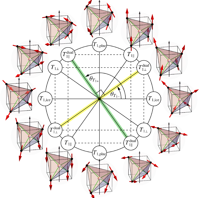
Figure 3: The mixing of the two $T_{1}$ irreps induces canting of the spins. The canting angle relative to the local easy axes, $\theta_{c}$, which decouples the two $T_{1}$ irreps is defined modulo $\pi/2$. Defining $\theta_{T_{1-}}$ as the canting angle of the lower-energy $T_{1}$ irrep, then $\theta_{T_{1+}}=\theta_{T_{1-}}+\pi/2$ is the canting angle of the higher-energy $T_{1}$ irrep, and these two angles are defined modulo $\pi$. There are some special canting angles which we note here: $T_{1,\text{ice}}$ corresponds to spins aligned in 2-in 2-out fashion along the easy axes, whose complement $\smash{T_{1,\text{planar}}}$ is ferromagnetic with spins orthogonal to the easy axes. $T_{1\parallel}$ is the colinear spin configuration along the global Cartesian axes ($\smash{\theta_{\smash{T_{1\parallel}}}=\cos^{-1}(1/\sqrt{3})}$), whose complement $\smash{T_{1\perp}}$ has all spins lying in a plane, c.f. Fig. 2(e,f). Each angle $\theta$ has a dual angle $-\theta$ corresponding to rotating all spins by $\pi$ about their local easy axes, which is the dual irrep when the sign of $J_{z\pm}$ is flipped.

II.4 $T_{1}$ Mixing and Canting Angle

Since there are two $T_{1}$ irreps they can have a symmetry-allowed coupling in the Hamiltonian and can therefore mix. The $\smash{T_{1\parallel}}$ and $\smash{T_{1\perp}}$ irrep order parameters derived from the multipole decomposition we will refer to as the global $T_{1}$ irreps, since they involve the components of spins relative to the global Cartesian axes. Their coupling in the Hamiltonian is of the form

$$H_{\smash{T_{1\parallel}}\oplus\smash{T_{1\perp}}}=\begin{pmatrix}\bm{m}_{\smash{T_{1\parallel}}}\\ \bm{m}_{\smash{T_{1\perp}}}\end{pmatrix}^{T}\begin{pmatrix}J_{\smash{T_{1\parallel}}}&J_{\smash{T_{1\parallel}}\cdot\smash{T_{1\perp}}}\\ J_{\smash{T_{1\parallel}}\cdot\smash{T_{1\perp}}}&J_{\smash{T_{1\perp}}}\end{pmatrix}\begin{pmatrix}\bm{m}_{\smash{T_{1\parallel}}}\\ \bm{m}_{\smash{T_{1\perp}}}\end{pmatrix},$$ (33)

where the cross term is controlled by the global $J_{3}$ parameter in Eq. 3 and the single ion anisotropy,

$$J_{\smash{T_{1\parallel}}\cdot\smash{T_{1\perp}}}=\frac{\sqrt{2}}{3}(J_{\text{SIA}}+3J_{3}),$$ (34)

which prefer for spins to cant away from the global Cartesian axes and towards the local three-fold axes. The amount of canting is determined by eliminating the coupling between the two $T_{1}$ irreps, which is achieved by defining rotated $T_{1}$ modes

$$\begin{pmatrix}\bm{m}_{T_{1\phi}}\\ \bm{m}_{T_{1\phi^{\prime}}}\end{pmatrix}=\begin{pmatrix}\cos\phi&\sin\phi\\ -\sin\phi&\cos\phi\end{pmatrix}\begin{pmatrix}\bm{m}_{\smash{T_{1\parallel}}}\\ \bm{m}_{\smash{T_{1\perp}}}\end{pmatrix}.$$ (35)

These rotated $T_{1}$ modes have a simple interpretation: each spin cants in one of the mirror planes according to

$${m}^{\alpha}_{T_{1\phi}}=\sum_{\mu}\underbrace{(\cos(\phi)\hat{\bm{e}}^{\alpha}+\sin(\phi)(\hat{\bm{\psi}}_{T_{1,\perp}}^{\alpha})_{\mu})}_{(\displaystyle\hat{\bm{\psi}}_{T_{1\phi}}^{\alpha})_{\mu}}\cdot\bm{S}_{\mu}.$$ (36)

and similarly for $T_{1\phi^{\prime}}$. The critical angle $\phi_{c}$ which decouples the two $T_{1}$ irreps is then given in terms of the global irrep parameters by solving the equation

$$\tan(2\phi_{c})=\frac{2J_{\smash{T_{1\parallel}}\cdot\smash{T_{1\perp}}}}{J_{\smash{T_{1\perp}}}-J_{\smash{T_{1\parallel}}}}.$$ (37)

Note that $\phi_{c}$ is only defined modulo $\pi/2$, i.e. it does not tell us whether the $T_{1}$ irrep with angle $\phi_{c}$ or $\phi_{c}+\pi/2$ has lower energy. Diagonalizing the matrix in Eq. 33 yields the energies of the decoupled $T_{1}$ normal modes

$$J_{T_{1\pm}}=\frac{1}{2}\left(J_{\smash{T_{1\parallel}}}+J_{\smash{T_{1\perp}}}\pm\sqrt{(J_{\smash{T_{1\parallel}}}-J_{\smash{T_{1\perp}}})^{2}+4{J_{\smash{T_{1\parallel}}\cdot\smash{T_{1\perp}}}}^{2}}\,\right),$$ (38)

where the $\pm$ indicates the higher or lower energy eigenvalue. For solutions of Eq. 37 in the range $\phi_{c}\in(-\pi/4,\pi/4)$, if $J_{\smash{T_{1\parallel}}}<J_{\smash{T_{1\perp}}}$ then $T_{1-}=T_{1\phi_{c}}$, while the opposite inequality implies $T_{1-}=T_{1\phi_{c}^{\prime}}$.

II.4.1 Easy-Axis Limit of $T_{1}$ Irreps

It is through canting and mixing the two $T_{1}$ irreps that one connects the global irreps to the local symmetry-adapted description in Eq. 5. Writing the canting angle equation Eq. 37 in terms of the local couplings,

$$\tan(2\phi_{c})=2\sqrt{2}-\frac{72J_{z\pm}}{2J_{\pm}+4J_{\pm\pm}+J_{zz}+16\sqrt{2}J_{z\pm}-J_{\text{SIA}}},$$ (39)

exposes a special critical angle—when $J_{z\pm}=0$ the canting angle is given by

$$\phi_{0}\equiv\tan^{-1}(2\sqrt{2})/2=\cos^{-1}(\sqrt{2/3}).$$ (40)

At this special canting angle, the local vectors in Eq. 36 are aligned along or orthogonal to the local three-fold axis $\hat{\bm{z}}_{\mu}$. This occurs precisely when $J_{z\pm}=0$, i.e. when the local $z$-components of the spin are completely decoupled from the local transverse components. We refer to the two corresponding irreps as

$$T_{1\phi_{0}}\equiv T_{1,\text{planar}},\quad T_{1\phi_{0}^{\prime}}\equiv T_{1,\text{ice}},$$ (41)

using the notation of Ref. [55]. The $T_{1,\text{ice}}$ irrep corresponds to the ground states of spin ice, with two spins pointing “in” and two spins pointing “out” of the tetrahedron. The $T_{1,\text{planar}}$ irrep corresponds to ferromagnetic configurations with spins in their local easy-planes. It is very useful to express the canting relative to the local easy axes rather than the global Cartesian axes, by defining

$$\theta=\phi-\phi_{0}.$$ (42)

The canting angle relative to the local axis that decouples the two $T_{1}$ irreps then satisfies the equation

$$\tan(2\theta_{c})=\frac{2J_{T_{1,\text{ice}}\cdot T_{1,\text{planar}}}}{J_{T_{1,\text{ice}}}\!-J_{T_{1,\text{planar}}}}=\frac{8J_{z\pm}}{2J_{\pm}+4J_{\pm\pm}+J_{zz}-J_{\text{SIA}}},$$ (43)

where the corresponding couplings are listed in Table 2. From this equation it is evident that switching the sign of $J_{z\pm}$ corresponds to switching the sign of $\theta_{c}$.

This is all summarized in Fig. 3, which shows the how the spin configuration of the $T_{1}$ irreps evolves as the canting angle rotates. To each configuration there is a corresponding dual configuration with the opposite sign of the canting angle, corresponding to a $\pi$ rotation of each spin about its local easy axis. For a given set of exchange parameters, one of the two $T_{1}$ irreps will have a lower energy, and we denote the corresponding angle by $\theta_{T_{1\pm}}$, in which case the higher energy irrep has angle $\theta_{T_{1+}}=\theta_{T_{1-}}+\pi/2$. These angles are defined modulo $\pi$, since a $\pi$ rotation returns to the same $T_{1}$ irrep with the spin orientations reversed, i.e. the time-reversed state.

Table 2: Irrep energies, Eq. 28, and $T_{1}$ couplings, Eq. 33, in terms of the global and local basis interaction parameters.

III Irrep Parameterization of the Model Space

In the remainder of this paper we will elucidate the structure of the full classical phase diagram of the nearest-neighbor spin-1/2 model on the pyrochlore lattice, focusing especially on the locations of the phase boundaries and the triple and quadruple points where three or four phases become degenerate, respectively. The irrep eigenvalues are given in Table 2. For a given set of parameters, the classical ground state is given by finding which irrep takes the minimum eigenvalue and aligning the spins along the associated ordering vectors in Eq. 17. For classical fixed-length vector spins this is the minimal energy state, and away from phase boundaries this should be an accurate product state ansatz for the quantum ground state. As we will see in detail, there are effectively four phases, one for each irrep if we don’t distinguish between the two $T_{1}$ irreps. Each phase is the locus of parameter space within which one irrep has the lowest energy and the others are separated by a gap. In order to map the phase diagram it is crucial to identify the locus of parameters along which multiple ground states are degenerate, i.e. phase boundaries, triple points, and quadruple points.

III.1 Irrep Parameterization and $J_{z\pm}$ Duality

Our strategy is to parameterize the phase diagram not in terms of the basis-dependent spin-spin couplings, but rather in terms of the basis-independent irrep energies $J_{I}$. To achieve this, we first invert the relations in Table 2 in order to obtain the couplings as functions of the irrep eigenvalues. The resulting equations are

$$J_{zz} =\frac{1}{12}[3J_{A_{2}}-2J_{E}-3J_{T_{2}}-3(J_{T_{1+}}+J_{T_{1-}})]$$ (44a)

$$J_{\pm} =-\frac{J_{E}}{6}$$ (44b)

$$J_{\pm\pm} =-\frac{1}{12}(J_{E}+3J_{T_{2}})$$ (44c)

$$|J_{z\pm}| =\frac{1}{12}\sqrt{-(2J_{E}+3J_{T_{2}}+3J_{T_{1+}})(2J_{E}+3J_{T_{2}}+3J_{T_{1-}})}$$ (44d)

$$J_{\text{SIA}} =\frac{1}{4}[J_{A_{2}}+2J_{E}+3J_{T_{2}}+3(J_{T_{1-}}+J_{T_{1+}})]$$ (44e)

For any model with a given sign of $J_{z\pm}$, there is another model with the opposite sign of $J_{z\pm}$ with the same irrep energies, because only its square appears in the irrep energies $J_{T_{1\pm}}$ in Table 2.

This corresponds to a duality transformation of the Hamiltonian: applying a $\pi$ rotation of each spin about its local $\hat{\bm{z}}_{i}$ axis sends $S_{i}^{\pm}\to-S_{i}^{\pm}$, changing the sign of the $S^{z}S^{\pm}$ term in Eq. 5 while leaving the rest of the terms invariant. This sign change can then be cancelled by changing the sign of $J_{z\pm}$. Furthermore, such a rotation maps each irrep back to itself: $A_{2}$ is clearly invariant under this transformation; for the easy-plane $E$ and $T_{2}$ configurations this sends a spin configuration to its time-reversed configuration; and $T_{1}$ configurations are turned into other $T_{1}$ configurations. As such, reversing the sign of $J_{z\pm}$ relates two Hamiltonians in the same phase. This is clear from Table 2 since the energies of the irreps are unchanged.

It is convenient to parameterize the splitting between the two $T_{1}$ irreps,

$$J_{T_{1\pm}}\equiv J_{T_{1}}\pm J_{\delta T_{1}}\quad\text{with}\quad J_{\delta T_{1}}\geq 0,$$ (45)

in order to write Eq. 44d in the form

$$|J_{z\pm}|=\frac{1}{12}\sqrt{(3J_{\delta T_{1}})^{2}-(2J_{E}+3J_{T_{2}}+3J_{T_{1}})^{2}}.$$ (46)

In this form we can see the close relation between $J_{z\pm}$ and the splitting of the two $T_{1}$ irreps. In particular, there is a constraint on the possible eigenvalues,

$$3J_{\delta T_{1}}\geq|2J_{E}+3J_{T_{2}}+3J_{T_{1}}|,$$ (47)

in order that $J_{z\pm}$ is real. It is evident that if the two $T_{1}$ irreps are degenerate ($J_{\delta T_{1}}=0$) then $J_{z\pm}$ must be zero, saturating the inequality. Equation 46 suggests that it is convenient to define a dimensionless parameter

$$\alpha\equiv\operatorname{sign}(J_{z\pm})\frac{(2J_{E}+3J_{T_{2}}+3J_{T_{1}})}{3J_{\delta T_{1}}},$$ (48)

so that

$$|J_{z\pm}|=\frac{J_{\delta T_{1}}}{4}\sqrt{1-\alpha^{2}},$$ (49)

such that the inequality Eq. 47 is equivalent to $|\alpha|\leq 1$. The sign prefactor in Eq. 48 has been chosen because it allows us to interpret the canting formula Eq. 43 geometrically. It simplifies to

$$\tan(2\theta_{c})=\frac{\sqrt{1-\alpha^{2}}}{\alpha}=\tan\left(\cos^{-1}(\alpha)\right),$$ (50)

from which we obtain the convenient formula

$$\theta_{c}=\frac{1}{2}\cos^{-1}(\alpha)=\cos^{-1}\left(\sqrt{\frac{\alpha+1}{2}}\right)\mod\pi/2.$$ (51)

Degenerate	Tuned	Parameterization	Range	Refs.
Irreps	Irreps
$A_{2}\oplus E\oplus T_{2}\oplus T_{1\perp}$	$T_{1\parallel}$	$J_{zz}=-\frac{1}{12}\Delta_{T_{1+}}$ $J_{\pm}=\frac{1}{24}\Delta_{T_{1+}}$ $J_{\pm\pm}=\frac{1}{12}\Delta_{T_{1+}}$ $|J_{z\pm}|=\frac{1}{6\sqrt{2}}\Delta_{T_{1+}}$	—	[26, 27]
$E\oplus T_{2}\oplus T_{1-}$	$A_{2}\oplus T_{1+}$	$J_{zz}=\frac{1}{36}(11\Delta_{A_{2}}-3\Delta_{T_{1+}})$ $J_{\pm}=\frac{1}{72}(\Delta_{A_{2}}+3\Delta_{T_{1+}})$ $J_{\pm\pm}=\frac{1}{36}(\Delta_{A_{2}}+3\Delta_{T_{1+}})$ $|J_{z\pm}|=\frac{1}{36}\sqrt{(3\Delta_{T_{1+}}-2\Delta_{A_{2}})(2\Delta_{A_{2}}+6\Delta_{T_{1+}})}$	$-3\leq{\displaystyle\frac{\Delta_{A_{2}}}{\Delta_{T_{1+}}}}\leq\frac{3}{2}$	[45]
$A_{2}\oplus T_{2}\oplus T_{1-}$	$E\oplus T_{1+}$	$J_{zz}=-\frac{1}{36}(2\Delta_{E}+3\Delta_{T_{1+}})$ $J_{\pm}=\frac{1}{72}(-10\Delta_{E}+3\Delta_{T_{1+}})$ $J_{\pm\pm}=\frac{1}{36}(-\Delta_{E}+3\Delta_{T_{1+}})$ $|J_{z\pm}|=\frac{1}{36}\sqrt{(6\Delta_{T_{1+}}-2\Delta_{E})(3\Delta_{T_{1+}}+2\Delta_{E})}$	$-\frac{3}{2}\leq\displaystyle\frac{\Delta_{E}}{\Delta_{T_{1+}}}\leq 3$	[44]
$A_{2}\oplus E\oplus T_{1-}$	$T_{2}\oplus T_{1+}$	$J_{zz}=-\frac{1}{12}(\Delta_{T_{2}}+\Delta_{T_{1+}})$ $J_{\pm}=\frac{1}{24}(\Delta_{T_{2}}+\Delta_{T_{1+}})$ $J_{\pm\pm}=\frac{1}{12}(\Delta_{T_{1+}}-2\Delta_{T_{2}})$ $|J_{z\pm}|=\frac{1}{12}\sqrt{(2\Delta_{T_{1+}}-\Delta_{T_{2}})(\Delta_{T_{1+}}+\Delta_{T_{2}})}$	$-1\leq\displaystyle\frac{\Delta_{T_{2}}}{\Delta_{T_{1+}}}\leq 2$
$A_{2}\oplus E\oplus T_{2}$	$T_{1-}\oplus T_{1+}$	$J_{zz}=-\frac{1}{12}\Delta_{T_{1}}$ $J_{\pm}=\frac{1}{24}\Delta_{T_{1}}$ $J_{\pm\pm}=\frac{1}{12}\Delta_{T_{1}}$ $|J_{z\pm}|=\frac{1}{12}\sqrt{(3\Delta_{\delta T_{1}})^{2}-\Delta_{T_{1}}^{2}}$	$-3\leq{\displaystyle\frac{\Delta_{T_{1}}}{\Delta_{\delta T_{1}}}}\leq 3$
$T_{2}\oplus T_{1,\text{ice}}\oplus T_{1,\text{plnr}}$	$E\oplus A_{2}$	$J_{zz}=\frac{1}{4}\Delta_{A_{2}}$ $J_{\pm}=-\frac{1}{8}\Delta_{A_{2}}$ $J_{\pm\pm}=0$ $J_{z\pm}=0$	$\Delta_{E}=\Delta_{A_{2}}$	[43]
$\phantom{A_{2}}\mathllap{E}\oplus T_{1,\text{ice}}\oplus T_{1,\text{plnr}}$	$T_{2}\oplus A_{2}$	$J_{zz}=\frac{1}{4}\Delta_{A_{2}}$ $J_{\pm}=\frac{1}{24}\Delta_{A_{2}}$ $J_{\pm\pm}=-\frac{1}{12}\Delta_{A_{2}}$ $J_{z\pm}=0$	$\Delta_{T_{2}}=\frac{2}{3}\Delta_{A_{2}}$	[47]
$A_{2}\oplus T_{1,\text{ice}}\oplus T_{1,\text{plnr}}$	$E\oplus T_{2}$	—	—

Table 3: List of fourfold and threefold degenerate models. There are two parameter combinations (up to an overall scale) yielding fourfold degeneracy, both of which have $T_{1\parallel}$ gapped: the Heisenberg antiferromagnet (HAFM) (with $J_{z\pm}>0$), and its $J_{z\pm}$-dual (with $J_{z\pm}<0$), denoted HAFM${}_{\text{dual}}$. By gapping one of the four degenerate irreps, we obtain four lines (up to a scale) along which three phases meet, which go from the HAFM, to $J_{z\pm}=0$, then return with the opposite sign of $J_{z\pm}$ to the HAFM${}_{\text{dual}}$. For the last line we used the $T_{1}$ splitting parameters defined in Eq. 57. The remaining three combinations of three degenerate irreps have both $T_{1}$ irreps degenerate, which is only possible when $J_{z\pm}=0$. Two of these combinations are possible, corresponding to isolated triple points (up to a scale) which do not lie on one of the four triple lines. There is one other possible combination of three degenerate and two gapped irreps, but it does not admit any solutions with real $J_{z\pm}$, because $A_{2}$ is the charge irrep for $T_{1\text{ice}}$, and their ground states are mutually incompatible (c.f. Fig. 11). We have given references for cases where examples have appeared previously in the literature (see Section VI.2 for details). Flat band degeneracies for all cases in this table are listed in Table 6. Note that reversing the signs of all couplings produces another set of models with triple degeneracies higher in the interaction matrix spectrum, c.f. Fig. 13.

III.2 Parameter Space vs. Model Space

Any real choice of the five symmetry-allowed nearest-neighbor spin-spin coupling parameters in Eq. 4 or Eq. 5, each a real number, defines an interaction matrix $\mathcal{J}$ and thus a Hamiltonian. We call this $\mathbbm{R}^{5}$ five-dimensional space the parameter space ($\mathbbm{R}^{4}$ if we set $J_{\text{SIA}}=0$). Within this space is a special point where all couplings are zero, corresponding to the trivial Hamiltonian $H=0$. Many of the remaining non-trivial parameter sets are physically equivalent up to an overall energy scale. Ideally one would like to parameterize the space of Hamiltonians modulo such rescalings, which we call the model space.

One way to parameterize the model space is to simply take a unit sphere in the parameter space, e.g. using the local couplings in Eq. 5 (setting $J_{\text{SIA}}=0$)

$$J_{zz}^{2}+J_{\pm\pm}^{2}+J_{z\pm}^{2}+J_{\pm}^{2}=1.$$ (52)

Of course one could alternatively take the unit sphere in the basis $J_{1}\cdots J_{4}$ in Eq. 2, or those in Eq. 4. The unit spheres in these spaces do not coincide, however, since the transformation relating these bases of the parameter space, Eqs. 7 and 8, are not orthogonal. The parameter space does not have a canonical metric to measure distances between parameter sets or to define orthogonality, so such a choice of sphere is arbitrary. In any case such a choice does not yield a useful parameterization of the space of models. In this section we provide a parameterization by directly manipulating the irrep energies.

In full generality, a model is an equivalence class of parameters, where two parameter sets are equivalent if the band structure of the interaction matrix $\mathcal{J}$ eigenvalues (i.e. the $J_{n}(\bm{q})$ in Eq. 11) differ by either a shift or a re-scaling, i.e. a changing of the total bandwidth of the band structure of $\mathcal{J}$ without changing the band structure. For nearest-neighbor interactions the band structure of $\mathcal{J}$ is completely determined by the $\bm{q}=\bm{0}$ eigenvalues, i.e. the irrep eigenvalues $J_{I}$. Therefore, a set of irrep eigenvalues determines an interaction matrix $\mathcal{J}$, with the caveats that (i) each allowed set of irrep eigenvalues corresponds to a pair of models with opposite signs of $J_{z\pm}$, and (ii) the inequality Eq. 47 must be satisfied for $J_{z\pm}$ to be real. Consider then the 5-dimensional space of real irrep eigenvalues $J_{I}$. We define an equivalence relation under affine rescalings

$$J_{I}\sim J_{I}^{\prime}\quad\text{if}\quad J_{I}^{\prime}=aJ_{I}+b$$ (53)

for some real numbers $a$ and $b$ with $a>0$. An equivalence class $[J_{I}]$ defines a model, and the space of equivalence classes is the model space, which has the topology of a 3-sphere.

III.3 Parameterizing the Model Space with $J_{\text{SIA}}=0$

In order to explore the model space, we require a parameterization which selects a single representative of each equivalence class of parameter sets, i.e. one which effectively fixes $a$ and $b$ in Eq. 53. To do so, we first choose an arbitrary energy scale $J_{0}$ and measure each irrep energy relative to it, defining

$$J_{I}=J_{0}+\Delta_{I}.$$ (54)

To fix $b$, we restrict the allowed parameter sets $\Delta_{I}$ to those for which $\mathrm{min}(\Delta_{I})=0$. In other words, we fix the energy scale to be $J_{0}=\mathrm{min}(J_{I})$, i.e. the ground state energy. In order to fix $a$ we have to fix the overall scale. Here many choices are possible, but the most obvious is to set $\mathrm{max}(\Delta_{I})=1$. In other words, we fix the total bandwidth of $\mathcal{J}$ to be unity, which is sensible because it is the natural energy scale in the Hamiltonian.

We note with this choice of scale, the $L^{2}$ norm on the space of real eigenvalues induces a dimensionless metric on the model space, which can (in principle) be used to define how far apart two models are from each other. While the parameter space does not have a canonical metric this would be the natural candidate for a “useful” metric—it measures how far apart two parameter sets are while holding the total bandwidth constant, i.e. modulo overall rescaling of the Hamiltonian. This may be a useful definition for quantitatively assessing how close a compound is to a phase boundary or a spin liquid [70].

For the purposes of this paper, we will set $J_{\text{SIA}}=0$, as is physically appropriate for spin-1/2 systems. This leads to helpful simplifications, but the analysis could be extended to include non-zero $J_{\text{SIA}}$. Setting Eq. 44e equal to zero and solving for $J_{0}$, we obtain

$$J_{0}=-\frac{1}{12}\left[\Delta_{A_{2}}+2\Delta_{E}+3\Delta_{T_{2}}+3(\Delta_{T_{1-}}+\Delta_{T_{1+}})\right].$$ (55)

Substituting back into the remaining four equations, we obtain

$$J_{zz} =\frac{1}{72}[11\Delta_{A_{2}}-2\Delta_{E}-3\Delta_{T_{2}}-3(\Delta_{T_{1-}}+\Delta_{T_{1+}})],$$ (56a)

$$J_{\pm} =\frac{1}{72}[\Delta_{A_{2}}-10\Delta_{E}+3\Delta_{T_{2}}+3(\Delta_{T_{1-}}+\Delta_{T_{1+}})],$$ (56b)

$$J_{\pm\pm} =\frac{1}{36}[\Delta_{A_{2}}-\Delta_{E}-6\Delta_{T_{2}}+3(\Delta_{T_{1-}}+\Delta_{T_{1+}})],$$ (56c)

$$|J_{z\pm}| =\frac{1}{36}\sqrt{(9\Delta_{\delta T_{1}})^{2}-[2\Delta_{A_{2}}-2\Delta_{E}-3\Delta_{T_{2}}+3\Delta_{T_{1}}]^{2}}$$ (56d)

where in Eq. 56d we have defined for convenience the equivalent of Eq. 45, the average and the splitting between the two $T_{1}$ irreps,

$$\Delta_{T_{1}}\equiv\frac{1}{2}(\Delta_{T_{1+}}+\Delta_{T_{1-}}),\quad\Delta_{\delta T_{1}}\equiv\frac{1}{2}(\Delta_{T_{1+}}-\Delta_{T_{1-}})\geq 0.$$ (57)

The full model space is parameterized by tuning the $\Delta_{I}$ subject to the constraints that

1. $\min\Delta_{I}=0$,

2. $\max\Delta_{I}=1$,

3. $\Delta_{T_{1}+}\geq\Delta_{T_{1-}}$,

4. $J_{z\pm}$ is real.

The model space is 3-dimensional, since at a generic point with one $\Delta_{I}$ set to zero and one set to unity there are three free parameters to vary. A phase is then the 3-dimensional locus of parameters where one of the $\Delta_{I}$ is zero and the rest are positive. While there are five $\Delta_{I}$ parameters, we will see there are only four distinct phases because the two $T_{1}$ irreps mix continuously. Phase boundaries are two-dimensional and occur when two $\Delta_{I}$ are zero while the remainder are positive. Triple points are one-dimensional lines along which three $\Delta_{I}$ are zero, one is fixed to unity, and the remaining one is allowed to vary. Lastly, it is possible to have a quadruple point, an isolated point where four phases are degenerate.

\begin{overpic}[width=429.28616pt]{param_variation_3-fold.pdf} \put(1.0,92.0){(a)} \put(1.0,66.0){(b)} \put(1.0,45.0){(c)} \put(1.0,23.3){(d)} \end{overpic}

Figure 4: Variation of (a) local couplings, (b) global couplings, (c) irrep energies, and (d) canting angle on the four triply-degenerate lines in the phase diagram listed in Table 3, characterized by tuning one of the irreps $I^{\prime}\in\{A_{2},E,T_{2},T_{1}\}$ while keeping the other three degenerate. (a) Local couplings for the parameterization of the Hamiltonian Eq. 5 computed from Eq. 56, with $J_{z\pm}<0$ indicated by the dashed line. Note that for the case $I^{\prime}=A_{2}$ (first column) we have scaled $J_{zz}$ by a factor of 2. (b) Global couplings in Eq. 3, with $J_{z\pm}<0$ indicated by the dashed lines. (c) Irrep eigenvalues $J_{I}$, with the triply degenerate eigenvalues denoted by a thick blue line, the tuned eigenvalue. (d) Evolution of the canting angles $\theta_{T_{1-}}$ (yellow) and $\theta_{T_{1+}}$ (green) with angles labeled according to Fig. 3, with $J_{z\pm}<0$ indicated by the dashed lines. The intersections of three phases, where three ground states are degenerate, occur for $\Delta_{I^{\prime}}/\Delta_{T_{1+}}>0$ and $\Delta_{T_{1+}}>0$ (blue region on the right side of each plot, c.f. Footnote 13). For $\Delta_{I^{\prime}}<0$ the irrep $I^{\prime}$ is the ground state but the other three are degenerate at higher energy (red region on the left side of each plot, c.f. Fig. 13(a)). Each of these triple lines forms a closed circle in the phase diagram (c.f. Fig. 13(a)). Columns are colored according to the irrep colors used in Figs. 5, 13, 7 and 13. The triple line $I^{\prime}=T_{1-}$ (last column) intersects the Heisenberg ferromagnet (HFM) and its $J_{z\pm}$-dual, where SO(3) rotational symmetry is restored, indicated by a black vertical line (c.f. Figs. 7 and 13).

IV Mapping the Phase Diagram

The parameterization of Eq. 56 allows us to efficiently explore the parameter space in a way that makes the phase boundaries and special subspaces manifest, while decoupling the rescaling dimension. We will visualize the phase diagram by stereographically projecting the 3-sphere Eq. 52 into 3-dimensional space using the mapping

$$(J_{zz},J_{\pm\pm},J_{z\pm},J_{\pm})\mapsto(X,Y,Z)\equiv\left(\frac{J_{zz}}{1-J_{\pm}},\frac{J_{\pm\pm}}{1-J_{\pm}},\frac{J_{z\pm}}{1-J_{\pm}}\right).$$ (58)

In particular, this 3-sphere has a 2-sphere subspace on which $J_{z\pm}=0$, dividing into into two hemispheres. Since the phases are dual under changing the sign of $J_{z\pm}$, the phase diagram in these two hemispheres is reflected through the $J_{z\pm}=0$ “equator”, i.e. the “northern” and “southern” hemispheres of the phase diagram are mirror images of each other. For completeness, the inverse mapping of Eq. 58 is given by

$$(X,Y,Z)\mapsto\frac{1}{R^{2}+1}\left(2X,2Y,2Z,R^{2}-1\right),$$ (59)

where $R^{2}=X^{2}+Y^{2}+Z^{2}$.

IV.1 Quadruple Points: Heisenberg Antiferromagnet

To map the structure of the phase diagram, we begin with the highest-degeneracy four-fold degenerate quadruple points. These can be searched for manually by setting all but one $\Delta_{I}$ to zero in Eq. 56 and checking whether solutions exist with real $J_{z\pm}$. This immediately rules out the possibility of fourfold degeneracies with only $A_{2}$, $E$, or $T_{2}$ gapped. This leaves only one possibility: $\Delta_{T_{1+}}>0$ and all others are zero. This corresponds to the Heisenberg antiferromagnet (HAFM) point, with Hamiltonian

$$H_{\text{HAFM}}\equiv E_{0}+\Delta_{T_{1+}}\sum_{t}|\bm{m}_{\smash{T_{1\parallel}}}|^{2}=\frac{\Delta_{T_{1+}}}{4}\sum_{\langle ij\rangle}\bm{S}_{i}\cdot\bm{S}_{j},$$ (60)

which has $J_{z\pm}>0$. The HAFM has a massively degenerate classical ground state manifold characterized by the zero-net-moment constraint $\bm{m}_{\smash{T_{1\parallel}}}=\bm{0}$ on every tetrahedron, corresponding to the large degeneracy of the irreps, a prototypical example of a classical spin liquid which has been extensively studied [71, 72, 73, 26, 74, 27, 28, 75, 76]. Since every model determined by a set of eigenvalues with $J_{z\pm}\neq 0$ has a dual with the opposite sign of $J_{z\pm}$, there is a second fourfold-degenerate point in the phase diagram which we will refer to as HAFM${}_{\text{dual}}$ [25]. The Hamiltonian at this point can be written as

$$H_{\text{HAFM}_{-}}\equiv E_{0}+\Delta_{T_{1+}}\sum_{t}|\bm{m}_{T_{1\parallel}^{\text{dual}}}|^{2},$$ (61)

where the gapped $\smash{T_{1\parallel}^{\text{dual}}}$ spin configuration, as well as the zero-energy $\smash{T_{1\perp}^{\text{dual}}}$, are shown in Fig. 3.

IV.2 Triple Lines and Points

Starting from the HAFM points where all four phase are degenerate, $\Delta_{A_{2}}=\Delta_{E}=\Delta_{T_{2}}=\Delta_{T_{1-}}=0$, one can lift the degeneracy of one of the four phases, thus tuning along a line where three phases are degenerate. The resulting parameter sets for these four triply degenerate lines are given in Table 3. For the ones where the gapped irrep is $I^{\prime}\in\{A_{2},E,T_{2}\}$, the line can be parameterized by the ratio $\Delta_{I^{\prime}}/\Delta_{T_{1+}}$. The fourth line where both $T_{1}$ irreps are gapped can be parameterized this way, but is better parameterized by the average and splitting of the two $T_{1}$ irreps, Eq. 57. The point $\Delta_{I^{\prime}}=0$ corresponds to the HAFM points, from which one can tune $\Delta_{I^{\prime}}/\Delta_{T_{1+}}$ continuously until it reaches a maximum allowed value at which $J_{z\pm}=0$. Each line then continues by reversing the sign of $J_{z\pm}$ and tuning $\Delta_{I^{\prime}}/\Delta_{T_{1+}}$ back to zero, ending at the other HAFM point. Figure 4 shows the evolution of (a) the local exchange couplings, (b) the global exchange couplings, (c) the irrep energies, and (d) the canting angle along these lines. The right side of each plot with blue background is the region where the the triply degenerate irreps are the ground state. The left side, with red background, has the triply degenerate irreps in the excited states, and is discussed further in Section VII.

There are three other possible combinations of three degenerate ground state irreps in which $\Delta_{T_{1-}}=\Delta_{T_{1+}}=0$ along with one other irrep. According to Eq. 46 this is only possible when $J_{z\pm}=0$. Two such cases are possible, when $\Delta_{E}=0$ or $\Delta_{T_{2}}=0$, corresponding to isolated triple points in the phase diagram. The third case with $\Delta_{A_{2}}=0$ has no solutions. This exhausts all possibilities for three irreps to be degenerate in the ground state.

\begin{overpic}[width=95.39693pt]{Jzpm0_2D_pair.pdf} \put(25.5,78.5){$A_{2}$} \put(20.0,40.0){$T_{2}$} \put(42.0,28.5){$E$} \put(16.5,16.0){$T_{1,\text{planar}}$} \put(20.0,90.0){$T_{2}$} \put(42.0,78.5){$E$} \put(16.5,67.0){$T_{1,\text{planar}}$} \put(0.0,97.0){\large{(a)}} \put(0.0,44.0){\large{(b)}} \end{overpic}

\begin{overpic}[width=333.88924pt]{Jzpm0_sphere.pdf} \put(52.0,-4.0){\large{(c)}} \put(79.0,30.0){\large{(d)}} \put(48.0,46.0){\large{$J_{\pm}$}} \put(31.0,32.0){\large{$J_{zz}$}} \put(26.0,24.0){\large{$J_{\pm\pm}$}} \put(65.0,8.3){\rotatebox{-27.0}{$J_{\pm\pm}=0$}} \put(16.5,9.5){\rotatebox{6.0}{$J_{zz}=0$}} \put(30.0,6.5){\rotatebox{-10.0}{$J_{\pm}=0$}} \put(0.0,21.0){\includegraphics[width=78.04842pt]{color_legend.pdf}} \put(0.0,44.0){\includegraphics[width=138.76157pt]{JT1_line_legend.pdf}} \put(62.0,27.0){\includegraphics[width=260.17464pt]{stereographic_projection.pdf}} \end{overpic}

Figure 5: The phase diagram restricted to $J_{z\pm}=0$. (a) Fixing $J_{zz}<0$ and varying $J_{\pm}$ and $J_{\pm\pm}$, three triple-points are indicated by black dots. The blue line indicates the locus on which the two $T_{1}$ irreps are degenerate defined by Eq. 62, i.e. along this line all canting angles in Fig. 3 are degenerate. (b) Fixing $J_{zz}>0$, again showing three triple points. The degenerate $T_{1}$ line (blue) separates the $T_{1,\text{planar}}$ from the $T_{1,\text{ice}}$ ground states, though they are continuously connected (i.e. in the same phase) out of the $J_{z\pm}=0$ phase. The intersection of this line with the phase boundary between the $T_{1}$ and either $T_{2}$ or $E$ phases yields the isolated triple points. (c) The two phase diagrams at left can be joined together by considering a unit 2-sphere in the 3-dimensional parameter space of $J_{zz}$, $J_{\pm}$, and $J_{\pm\pm}$, shown here. The $T_{1,\text{ice}}$ phase is on the back of the sphere. In order to visualize the entire surface of the sphere we perform a stereographic projection (illustrated in (d) inset) onto the flat plane. Here we show a disk corresponding to $J_{\pm}\leq 0.53$. The excluded region corresponding to the northern cap of the sphere, see inset (d), is always in the $E$ phase.

IV.3 The $J_{z\pm}=0$ Plane: Stereographic Projection

Since the model space is a 3-sphere, the $J_{z\pm}=0$ locus may be thought of as the “equator”, with the topology of a 2-sphere. It divides the 3-sphere into northern and southern hemispheres which are dual to each other under changing the sign of $J_{z\pm}$ and performing a $\pi$ spin rotation about the local axes. Within the $J_{z\pm}=0$ subspace this spin-rotation duality is promoted to a symmetry. Within this subspace there is an additional duality: performing a $\pi/2$ rotation of each spin about the local $\hat{\bm{z}}_{i}$ sends $\cramped{S_{i}^{\pm}\to\mp iS_{i}^{\pm}}$, which can be compensated by switching the sign of $J_{\pm\pm}$ [25]. Unlike the duality switching the sign of $J_{z\pm}$ discussed in Section III.1, which relates two parameter sets in the same phase, reversing the sign of $J_{\pm\pm}$ relates different phases since it changes the irrep energies in Table 2. Referring to the ground states in Fig. 2 and Fig. 3, the $J_{\pm\pm}$ duality switches $\psi_{2}\leftrightarrow\psi_{3}$ and $T_{2}\leftrightarrow T_{1,\text{planar}}$. However, it ensures that the phase boundaries will be symmetric across $J_{\pm\pm}=0$ within the $J_{z\pm}=0$ subspace. This duality is promoted to a symmetry when $J_{\pm\pm}=J_{z\pm}=0$.

Within the $J_{z\pm}=0$ subspace, the relevant couplings are $J_{zz}$, $J_{\pm}$, and $J_{\pm\pm}$, meaning that there is no direct coupling between the local easy-axis and easy-plane spin components. The ground states are therefore either easy-axis Ising orders (ferro- or antiferromagnetic), or easy-plane XY orders. The Ising ferromagnetic order occurs for dominant $\cramped{J_{zz}\ll 0}$ and corresponds to the $A_{2}$ all-in-all-out order. The Ising anti-ferromagnetic state occurs in the opposite limit $\cramped{J_{zz}\gg 0}$, corresponding to the $T_{1,\text{ice}}$ ground states. For dominant $\cramped{J_{\pm}\gg 0}$ the $E$ irrep is the ground state. Further selection of the energetically degenerate $\psi_{2}$ and $\psi_{3}$ configurations occurs due to order-by-disorder induced by spin wave fluctuations about the ground state. Lastly, large $\cramped{J_{\pm\pm}\gg 0}$ selects the $T_{2}$ order, while large $\cramped{J_{\pm\pm}\ll 0}$ selects the $T_{1,\text{planar}}$ configurations. Since $J_{zz}=0$ is a degenerate case where the Hamiltonian becomes a pure XY model, it is standard to use $J_{zz}$ as the energy scale, considering two separate cases depending on the sign of $J_{zz}$, while varying the ratios $\cramped{J_{\pm}/|J_{zz}|}$ and $\cramped{J_{\pm\pm}/|J_{zz}|}$. This yields the two phase diagrams in Fig. 5(a) and (b).

\begin{overpic}[width=117.07924pt]{phase_diagram_3D_top_down.pdf} \put(45.2,83.2){\rotatebox{90.0}{\tiny{$J_{zz}<0$}}} \put(51.5,83.2){\rotatebox{90.0}{\tiny{$J_{zz}>0$}}} \put(83.0,52.0){\rotatebox{0.0}{\tiny{$J_{\pm\pm}>0$}}} \put(83.0,46.5){\rotatebox{0.0}{\tiny{$J_{\pm\pm}<0$}}} \put(58.2,28.8){\rotatebox{45.0}{\tiny{$J_{\pm}<0$}}} \put(63.5,25.0){\rotatebox{45.0}{\tiny{$J_{\pm}>0$}}} \put(5.0,128.0){\rotatebox{0.0}{\footnotesize{$J_{z\pm}<0$}}} \put(5.0,165.0){\rotatebox{0.0}{\footnotesize{$J_{z\pm}>0$}}} \put(0.0,107.0){\includegraphics[width=164.77771pt]{phase_diagram_3d_stereographic.pdf}} \put(40.0,180.0){\tiny{${A_{2}}$}} \put(53.0,124.0){\tiny{${T_{1-}}$}} \put(68.0,173.0){\tiny{${E}$}} \put(95.0,117.0){\tiny{${T_{2}}$}} \put(10.0,190.0){(a)} \put(10.0,100.0){(b)} \put(170.0,190.0){(c)} \end{overpic}

\begin{overpic}[width=294.85841pt]{phase_diagram_3d.pdf} \put(40.0,-2.0){HAFM${}_{\text{dual}}$} \put(43.0,77.0){HAFM} \put(21.0,42.0){$A_{2}$ phase} \put(55.0,45.5){$T_{2}$ phase} \put(84.0,42.0){$E$ phase} \put(47.0,33.0){$T_{1}$ phase} \put(17.0,45.5){\rotatebox{73.0}{\small{$\Delta_{T_{2}}\!>0$}}} \put(28.6,53.5){\rotatebox{73.0}{\footnotesize{$\Delta_{T_{1-}}\!\!>0$}}} \put(44.2,52.0){\rotatebox{85.0}{\small{$\Delta_{E}>0$}}} \put(66.3,62.3){\rotatebox{-53.0}{\small{$\Delta_{A_{2}}\!>0$}}} \put(57.0,37.5){\scriptsize{pHAFM}} \put(86.0,56.0){\includegraphics[width=34.69038pt]{color_legend.pdf}} \put(72.0,0.0){\includegraphics[width=73.7146pt]{JT1_line_legend.pdf}} \put(18.5,3.8){$X$} \put(8.5,12.0){$Y$} \put(3.5,20.0){$Z$} \end{overpic}

Figure 6: The full phase diagram, including the four 3-fold degenerate lines which run from the HAFM to the HAFM${}_{\text{dual}}$models, crossing through the plane with $J_{z\pm}=0$. (a) Stereographically projected triple lines listed in Table 3, which pass through the $J_{z\pm}=0$ plane. Phases in the plane are colored the same as in Fig. 5, and the triply-degenerate lines are colored according to which of the four irreps is gapped along with $T_{1+}$. Above (below) the plane corresponds to $J_{z\pm}$ positive (negative). (b) A top-down view of (a), with the $J_{zz}=0$, $J_{\pm}=0$, and $J_{\pm\pm}=0$ lines indicated. (c) A “cartoon” version of the projection where we have “straightened out” the lines and phase boundaries to emphasize the topology of the phase diagram. The $J_{z\pm}=0$ plane is shown along with the four triple lines as in (a) and (b), along with the phase boundaries. Each phase has three boundaries, one with each of the other phases. The exterior region of the diagram is in the $E$ phase. The $A_{2}$ and $T_{2}$ phases are enclosed by the yellow and blue phase boundaries, respectively. When turning on $J_{z\pm}\neq 0$ there is only a single contiguous $T_{1}$ phase, indicated by the red phase boundary. The $J_{z\pm}>0$ portion of the $T_{1}\oplus E$ phase boundary is not shown in order to expose the interior region of the $T_{1}$ phase and its phase boundaries with the $A_{2}$ and $T_{2}$ phases. An undistorted version of the phase boundaries according to the stereographic projection Eq. 58 is shown in Fig. 7.

Within these two diagrams one can clearly distinguish six triple points where three phases are degenerate, corresponding to the four lines and two special points that we identified in Table 3. The two special points occur when both $T_{1}$ irreps are degenerate, at the ends of the line separating the $T_{1,\text{planar}}$ and $T_{1,\text{ice}}$ regions of the phase diagram. As we saw from Eq. 46, the degeneracy of the two $T_{1}$ irreps is only possible when $J_{z\pm}=0$, and meaning that there is no phase boundary between two distinct $T_{1}$ phases when $J_{z\pm}\neq 0$, i.e. there is only a single $T_{1}$ phase. It is therefore interesting to identify the locus on which the two $T_{1}$ irreps are degenerate, i.e. all canting angles in Fig. 3 are degenerate, which is contained within the $J_{z\pm}=0$ subspace. From Table 2 (setting $J_{\text{SIA}}=0$) this occurs when the square root which splits to the two $T_{1}$ energies is zero, i.e. when

$$2J_{\pm}+4J_{\pm\pm}+J_{zz}=0\quad\text{and}\quad J_{z\pm}=0\quad(J_{T_{1+}}=J_{T_{1-}}).$$ (62)

The solution of this equation is shown by the blue line in Fig. 5(a,b). Along this line all canted $T_{1}$ configurations in Fig. 3 are degenerate.

In order to unify Fig. 5(a) and (b) into a single two-dimensional phase diagram, we consider the unit sphere in the space spanned by $J_{\pm\pm}$, $J_{zz}$, and $J_{\pm}$. This is the “equator” of the 3-sphere defined by Eq. 52. This 2-sphere is shown in Fig. 5(c), with the phases colored the same as in Fig. 5a,b. In this figure the $T_{1,\text{ice}}$ region is on the back of the sphere and not visible. In order to visualize the entire surface of the sphere, we use the stereographic map defined by Eq. 58 to project the surface of the sphere onto a plane. The inset Fig. 5(d) illustrates how stereographic projection maps the surface of the sphere to a plane. We have chosen the azimuthal axis to be the $J_{\pm}$ axis, which becomes the radial direction on the projected surface. The top of the sphere is in the $E$ phase, so that after projecting onto a plane all of the phase boundaries appear near the origin, surrounded by the large-$J_{\pm}$ $E$ phase, which extends to infinity.

IV.4 Big Picture: The Full Phase Diagram

We now have all the pieces to put together the full phase diagram using the stereographic projection Eq. 58 from the 3-sphere to 3-dimensional euclidean space. Using the projected $J_{z\pm}=0$ plane from Fig. 5 as our baseline, turning on $J_{z\pm}$ takes us into the third (vertical) dimension. First, Footnote 13(a,b) adds to the $J_{z\pm}=0$ plane the four triple lines, along each of which three irreps are degenerate and one is gapped. They are labeled and colored according to which irrep is gapped along that line with Footnote 13(a) showing an edge-one perspective and (b) showing a top-down view. All four meet at the two HAFM points above and below the plane, with the region above (below) this plane corresponding to $J_{z\pm}$ positive (negative). The HAFM sites below the plane while its dual sits above the plane.

In order to visualize the phase boundaries in this three-dimensional space in a static two-dimensional image, it is convenient to deform the phase diagram in order to “straighten out” the four triple lines. We thus provide the topologically equivalent and simpler to visualize picture shown in Footnote 13(c). By choosing the “point at infinity” to be deep in the $E$ phase, all of the phase boundaries are located near the origin, and the exterior region is all in the $E$ phase. We could have chosen the point at infinity to be deep within any of the four phases, and obtained a qualitatively similar phase diagram with the other three phases located near the origin. We have colored the phase boundaries surrounding the $A_{2}$ phase yellow, those surrounding the $T_{2}$ phase blue, and those surrounding the $T_{1}$ phase red. Gridlines on the phase boundaries are added as guides to the eye to emphasize the 3-dimensionality of the surfaces, but do not have any special meaning. We have excluded the $J_{z\pm}>0$ phase boundary between the $T_{1}$ phase and the $E$ phase in order to show the interior region of the $T_{1}$ phase and expose its phase boundaries with the $A_{2}$ and $T_{2}$ phases along with their triple line. Each of the four phases is enclosed by three phase boundaries where it touches one of the other phases. The $J_{z\pm}\geq 0$ region of each phase is topologically equivalent to a tetrahedron, and the same for the $J_{z\pm}\leq 0$ region, thus each phase has the topology of two tetrahedra glued along a triangular face. Footnote 13 constitutes a primary result of this work: a complete picture of the pyrochlore phase diagram showing all of the phases, phase boundaries, triple lines, and quadruple points.

V Topological Canting Cycles

In this section we investigate the locus on which the two $T_{1}$ irreps are degenerate, defined by Eq. 62. Whereas the energetic crossing of two different irreps in the ground state implies a phase transition, there is only one $T_{1}$ phase in which the canting angle varies continuously, so the crossing of the $T_{1}$ irreps is not a phase transition. This is a type of level repulsion: in order to make the square root zero in the last row of Table 2, we have to tune two separate parameter sets to be zero. In Footnote 13 one can see that the locus where the two $T_{1}$ irreps are degenerate (blue arc in the $J_{z\pm}=0$ plane) “pierces” each of the $T_{1}\oplus T_{2}$ and $T_{1}\oplus E$ phase boundaries once, giving rise to the two isolated triple points in the phase diagram. It passes within the $T_{1}$ phase as a special line of degeneracy along which all canting angles are degenerate in the ground state, but it does not form a phase boundary. We have indicated with a small black loop a path surrounding the line of $T_{1}$ degeneracy entirely contained within the $T_{1}$ phase. Moving along such a loop, one $T_{1}$ irrep is the unique ground state and the other is gapped, while the canting angle varies continuously. In other words the eigenvectors of the interaction matrix rotate in the $T_{1}$ subspace, going around the cycle shown in Fig. 3. Starting from a point with $T_{1-}=T_{1,\text{ice}}$ ($\theta_{T_{1-}}=0)$ and $T_{1+}=T_{1,\text{planar}}$, going halfway around the loop the canting angle continuously rotates by $\pi/4$ until the two $T_{1}$ irreps have swapped, then continuing around the ground state returns to $T_{1,\text{ice}}$ but with the opposite orientation of spins, i.e. a $\pi$ rotation in Fig. 3. This is an indication that the phase diagram has some interesting extra structure beyond the energetics of the phases, which we investigate further in this section.

V.1 Two Families of Hamiltonians

To investigate the canting behavior in more detail, as well as to illustrate the utility of having a complete phase diagram, we consider two particular one-parameter models—one which has constant canting angle and one on which the canting angle winds—and show how they fit in and are related in the phase diagram. Figure 7 shows the same phase diagram as Footnote 13(a,b), but with the “true” phase boundaries computed from the stereographic projection, rather than the deformed version shown in Footnote 13(c). Note in particular that the $T_{1}$ phase appears larger than the $A_{2}$ and $T_{2}$ phases—while the $T_{1}$ and $T_{2}$ phases are symmetric in the $J_{z\pm}=0$ plane, as seen in Footnote 13(b), turning on $J_{z\pm}\neq 0$ promotes the $T_{1}$ phase, which is the ground state in the large-$|J_{z\pm}|$ limit.

The first family is what we will call the Heisenberg-plus-$J_{z\pm}$ model, by tuning both $J_{\text{Heis}}$ from Eq. 4 and $J_{z\pm}$ from Eq. 5. Up to an overall scale, this is a 1-parameter family of Hamiltonians, which can be parameterized as $J_{\text{Heis}}=\cos\theta$ and $J_{z\pm}=\sin\theta$. This family is interesting because it corresponds to the triple line with $A_{2}$, $E$ and $T_{2}$ degenerate, while both $T_{1}$ irreps are tuned—the last triple line in Table 3 and the last column in Fig. 4. It is shown by the red circle in Fig. 7, which passes through both the Heisenberg ferromagnet (HFM) and anti-ferromagnet (HAFM) points, along with both of their duals. Part of this line lies on the triple intersection of the $A_{2}$, $E$, and $T_{2}$ phases, while the remainder passes through the $T_{1}$ phase. Since this family encloses the line where both $T_{1}$ irreps are degenerate, the canting angle winds by $\pi$ as we go around it while the two $T_{1}$ irrep energies never cross, as seen in the last column of Fig. 4(c) and (d).

The second model is the Heisenberg-plus-Dzyloshinskii-Moriya (H+DM) model [77, 78, 79, 57], which was recently studied in detail in Ref. [57], with Hamiltonian

$$H_{\text{H}+J_{z\pm}}=\sum_{\langle ij\rangle}(J_{\text{Heis}}\bm{S}_{i}\cdot\bm{S}_{j}+J_{\text{DM}}\bm{D}_{ij}\cdot\bm{S}_{i}\times\bm{S}_{j}).$$ (63)

This is a 1-parameter family of model up to a scale, which can be parameterized by $J_{\text{Heis}}=\cos\theta$ and $J_{\text{DM}}=\sin\theta$. This family is experimentally interesting because it is believed that the DM interaction should be the leading correction to the Heisenberg interaction in transition-metal pyrochlore insulators [57]. The resulting family is shown by the green circle in Fig. 7. Starting from the HAFM, it enters the $A_{2}$ phase, passes through the $A_{2}\oplus T_{1}$ phase boundary into the $T_{1}$ phase, meets the HFM point, then meets the isolated triple point on the $T_{1}\oplus E$ phase boundary (studied in more detail in Ref. [47] where it was dubbed the dipolar-quadrupolar-quadrupolar or “DQQ” point), then lies along the $T_{1}\oplus E$ phase boundary until it meets the HAFM again. This model is particularly interesting because it has $J_{3}=0$, meaning that the canting angle is constant for this model and the $T_{1}$ irreps decouple into $\smash{T_{1\parallel}}$ and $\smash{T_{1\perp}}$. For this model the two $T_{1}$ irreps cross each other when it crosses the locus where the two $T_{1}$ irreps are degenerate (blue line in Fig. 7): on the side with $J_{z\pm}>0$ we have $\Delta_{\smash{T_{1\parallel}}}<\Delta_{\smash{T_{1\perp}}}$, while on the side with $J_{z\pm}<0$ we have $\Delta_{\smash{T_{1\parallel}}}>\Delta_{\smash{T_{1\perp}}}$.

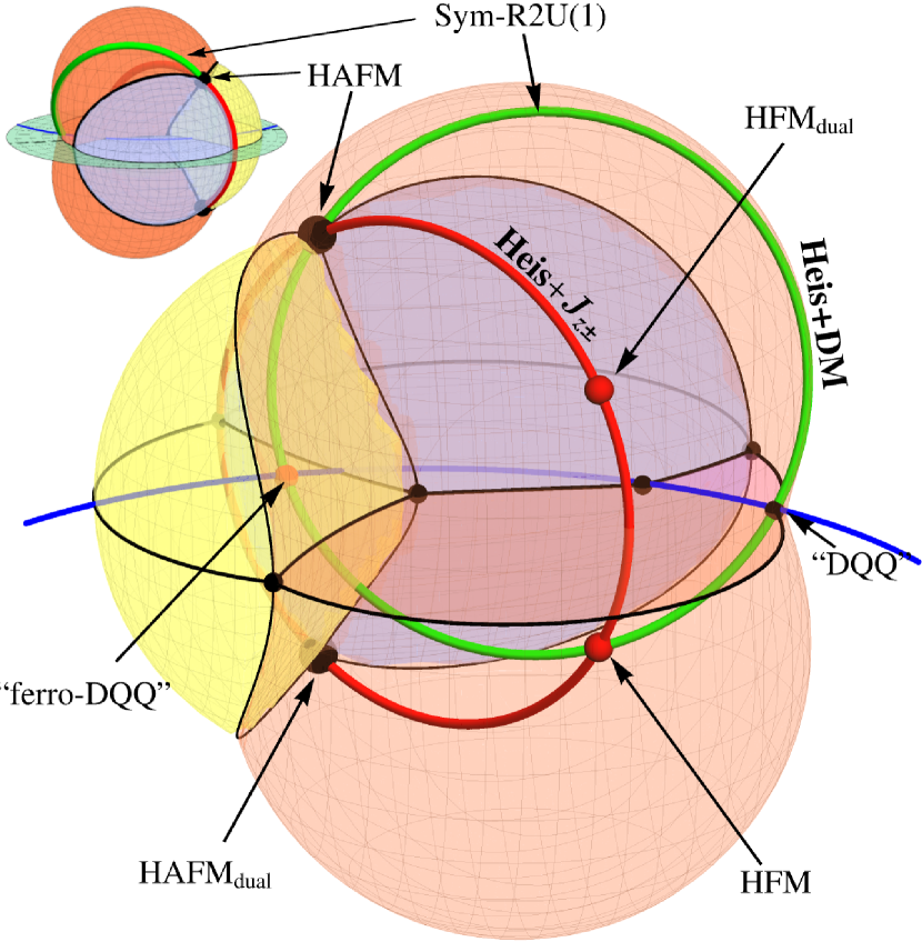
Figure 7: Here we show the “true” 3D stereographically projected phase diagram from Footnote 13(a,b) with the actual phase boundaries indicated, whereas Footnote 13(c) showed a deformed version that emphasized the topology. The inset (top right) shows the same from the back side. Here we have colored the triple lines black, along with the intersections of the phase boundaries with the $J_{z\pm}=0$ plane. The red circle is the Heisenberg-plus-$J_{z\pm}$ family, which corresponds to the triple line along which $A_{2}$, $E$, and $T_{2}$ are degenerate (last column of Fig. 4), which contains the Heisenberg anti-ferromagnet (HAFM), the Heisenberg ferromagnet (HFM), and both of their $J_{z\pm}$-duals. The green circle is the Heisenberg-plus-Dzyloshinskii-Moriya (H+DM) family [46, 57, 80], which passes through the HAFM, the HFM, the “DQQ” isolated triple point and its ferromagnetic counterpart. Because this family has $J_{3}=0$, it lies on a surface of constant canting where the $T_{1}$ irreps decompose as $\smash{T_{1\parallel}}\oplus\smash{T_{1\perp}}$. This surface can be parameterized as a sphere in the $J_{1}$-$J_{2}$-$J_{4}$ space, corresponding to $\alpha=1/3$ in Fig. 8. Along an arc from the DQQ point to the HAFM the H+DM model runs along the intersection of this constant-canting surface and the $E\oplus T_{1}$ phase boundary (red) where the ground state irreps are $E\oplus\smash{T_{1\perp}}$ which form a symmetric trace-free tensor, which was studied in Ref. [46].

\begin{overpic}[width=433.62pt]{canting_foliation.pdf} \put(3.0,39.0){(a)} \put(43.0,39.0){(b)} \put(18.0,43.0){\scriptsize$\alpha=1/3$} \put(33.0,35.0){\scriptsize$\alpha=0$} \put(26.0,7.0){\scriptsize$\alpha=-1/6$} \put(16.0,5.5){\scriptsize$\alpha=-1/3$} \put(7.0,6.5){\scriptsize$\alpha=-1/2$} \put(3.0,9.5){\scriptsize$\alpha=-2/3$} \put(0.0,13.5){\scriptsize$\alpha=-5/6$} \put(0.0,20.5){\scriptsize$|\alpha|=1$} \end{overpic}

Figure 8: Illustration of how the phase diagram is foliated into surfaces of constant canting angle, which are spheres that intersect along the locus where the two $T_{1}$ irreps are degenerate. Here we parameterize the canting angle using the parameter $\alpha$ in Eq. 51. (a) The 3D stereographically projected phase diagram from Footnote 13(a,b), along with the full circular locus of $T_{1}$ degeneracy (blue circle). For various canting angles we show a portion of the corresponding surface of constant canting (c.f. the color legend on the right). Each such surface is a sphere, which we have cut open for visualization. All of these surfaces intersect on the circular locus where the two $T_{1}$ irreps are degenerate and all canting angles have the same energy. (b) The same but for a two-dimensional slice of the phase diagram which intersects the locus of $T_{1}$ degeneracy at two points (blue circles with white borders). The $T_{1,\text{ice}}$ regime is a short pink line with white border extending from the right blue dot towards the right phase boundary. A black loop with arrowhead indicates a path in the parameter space that encloses the locus of $T_{1}$ degeneracy within the $T_{1}$ phase, about which the ground state evolves halfway around Fig. 3. Note that the $\alpha=1/3$ surface corresponds to $\smash{T_{1\parallel}}\oplus\smash{T_{1\perp}}$ decoupling, while $|\alpha|=1$ corresponds to $T_{1,\text{ice}}\oplus T_{1,\text{planar}}$, whose corresponding sphere is the $J_{z\pm}=0$ plane.

V.2 Surfaces of Constant Canting

Since the condition for the decoupling into $\smash{T_{1\parallel}}$ and $\smash{T_{1\perp}}$ to occur is that $J_{3}=0$, the one-dimensional H+DM family can be extended to a two-dimensional family on which the canting angle is constant by tuning the $J_{2}$ coupling in Eq. 3 (or the Kitaev-like coupling in Eq. 4). This family can be parameterized by the unit sphere in the $J_{1}$-$J_{2}$-$J_{4}$ parameter space, meaning that it is a 2-sphere in the phase diagram which intersections the circular $T_{1}$-degenerate locus, only part of which is shown in Footnotes 13 and 7 by the blue arc. On the $J_{z\pm}$ positive (negative) side of this sphere the lower-energy $T_{1}$ irrep is $\smash{T_{1\parallel}}$ ($\smash{T_{1\perp}}$).

For any canting angle $\theta$ there is a corresponding 2-sphere on which the canting angle is constant, given by the intersection of the 3-sphere Eq. 52 and the linear subspace satisfying equation Eq. 43, written as

$$\tan(2\theta)(2J_{\pm}+4J_{\pm\pm}+J_{zz})-8J_{z\pm}=0.$$ (64)

Thus the entire 3-sphere phase diagram is foliated into 2-sphere subspaces which intersect each other on the locus where the two $T_{1}$ irreps are degenerate defined by Eq. 62. Along any path on such a surface that crosses this line the energies of the two $T_{1}$ irreps cross each other. In particular, the $J_{z\pm}=0$ 2-sphere in Fig. 5 is the constant-canting surface with $\theta=0$, and the blue line divides it into two halves on which $T_{1-}$ is either $T_{1,\text{ice}}$ or $T_{1,\text{planar}}$.

This foliation of the phase diagram is illustrated in Fig. 8. We use the convenient parameter $\alpha\in[-1,1]$ defined in Eq. 48 to parameterize the canting angle as in Eq. 51. Note that $\alpha=1/3$ corresponds to the decomposition $\smash{T_{1\parallel}}\oplus\smash{T_{1\perp}}$, and $|\alpha|=1$ corresponds to $T_{1,\text{ice}}\oplus T_{1,\text{planar}}$. Figure 8(a) shows a collection of constant-canting 2-spheres for different values of $\alpha$, each of which is only partially shown to make the foliation structure visible. A cross section of the phase diagram is shown in Fig. 8(b) with various constant-canting surfaces indicated, demonstrating how the phase diagram is foliated. We can treat $\alpha$ as a periodic variable, identifying $\alpha=-1$ and $\alpha=1$, since both values result in the same surface. However, if we think of the spheres as being oriented, then going once around the $\alpha$ cycle reverses the orientation of the sphere, meaning one must go around the cycle twice to get back to the original orientation. Correspondingly, following a path like the black loop with an arrow in Fig. 8(b) that stays within the $T_{1}$ phase, the ground state angle $\theta_{T_{1-}}$ winds by $\pi$ in Fig. 3 rather than $2\pi$. If the system were adiabatically transported around such a cycle it would return to the same ground state but with all spins reversed.

V.3 “Diabolical” Loci from Duplicate Irreps

The line on which the two $T_{1}$ irreps are degenerate is analogous to so-called “diabolical loci” [58] and “unnecessary criticality” [59, 60, 61, 62]. These are gapless manifolds contained inside a single gapped phase, rather than on a phase boundary. They can be characterized by higher Berry phase topological invariants in the space of couplings, which classify generalized Thouless pumping cycles that transport symmetry charges across a system [81, 82, 83]. By a bulk-boundary correspondence they generally imply the existence of boundary phase transitions in the phase diagram  [83, 84].

While those studied examples generally have the critical surface completely contained inside a single phase, here we have a line which bridges between two phase boundaries. Nonetheless, the winding of the canting angle around this line may be analogous to a symmetry charge pump. The phenomenon occurs here due to the presence of multiple copies of a single irrep, as a kind of level repulsion between the corresponding eigenvalues. Whereas tuning to a phase boundary requires tuning only a single parameter, making the two $T_{1}$ irreps degenerate, i.e. setting $J_{T_{1+}}=J_{T_{1-}}$ from Table 2, requires tuning two independent parameters. Thus the locus is one dimension lower than the phase boundary. This guarantees the existence of a locus where the two $T_{1}$ irreps are degenerate which is not itself a phase boundary, around which the corresponding eigenvectors of the interaction matrix wind.

This phenomenon should be quite common in the phase diagrams of quadratic corner-sharing-cluster Hamiltonians (i.e. those on line graph lattices [28]), and we sketch here the basic idea. Performing a symmetry decomposition for all the spins in a cluster into irreducible representations will result in $d$ distinct irreps $I$, each with multiplicity $n_{I}$. The total number of symmetry-allowed tuning parameters must be equal to the total number of distinct copies of irreps, $D=\sum_{I=1}^{d}n_{I}$, meaning that the model space is topologically a $(D-1)$-sphere. There should be a single $(D-1)$-dimensional phase for each distinct irrep appearing in the decomposition, because all duplicates of an irrep are allowed to couple and can be continuously rotated into each other. For $n_{I}$ copies of an irrep one must perform an SO($n_{I}$) rotation in the irrep eigenspace to decouple them, meaning that there will be $n_{I}(n_{I}-1)/2$ “canting angles” parameterizing elements of $\mathrm{SO}(n_{I})$. Note that, because the irrep eigenvectors are only defined up to an overall sign, we actually only need an element $\mathrm{PSO}(n_{I})\simeq\mathrm{SO}(n_{I})/\mathbbm{Z}_{2}$. At a generic point in the phase one copy of the irrep has the lowest energy, and the canting angles vary continuously as the parameters are tuned. One then expects critical loci within the phase where multiple copies of the irrep are degenerate. A dimension $d_{l}$ locus can then be linked by a $(D-1)-d_{l}-1$-sphere, resulting in a topological winding cycle characterized by an element of the homotopy group $\pi_{D-d_{l}-2}(\mathrm{PSO}(n_{I}))$.

In the case of the pyrochlore studied here with zero single ion anisotropy we have $D=4$, $d_{l}=1$, and $n_{I}=2$, meaning that a 1-parameter family of Hamiltonians carries a $\pi_{1}(\mathrm{PSO}(2))\simeq\mathbbm{Z}$ winding number which counts how many times $2\theta_{c}$ winds around the $T_{1}$-degenerate locus. We can in principle define a Berry connection in the parameter space whose holonomy measures the winding,

$$a_{\mu}\propto\langle\psi_{\bm{0},T_{1-},\alpha}|\frac{\partial}{\partial{J_{\mu}}}|\psi_{\bm{0},T_{1-},\alpha}\rangle,$$ (65)

where $|\psi_{\bm{0},T_{1-},\alpha}\rangle$ is one of the $\bm{q}=\bm{0}$ eigenvector of the interaction matrix corresponding to the lowest-energy $T_{1}$ irrep (the result is independent of $\alpha$), and $J_{\mu}$ indicates the $\mu$’th coupling parameter. It is notable that within the $T_{1}$ phase a 1-parameter family with non-zero topological index must cross through the $T_{1,\text{ice}}$ surface where the system is a deconfined spin liquid, but it is unclear if this should be a generic property of such canting cycles. Outside the $T_{1}$ phase the line of degeneracy and the topological invariant associated to 1-dimensional families of Hamiltonians is well-defined, even though the $T_{1}$ irreps are not in the ground state. A signature of this degeneracy is likely to be identifiable in the magnon spectrum within the other phases. We leave the study of such topological winding cycles in the phase diagrams of classical spin models for future study.

VI Flat Band Degeneracies

We lastly turn to tabulating the flat band degeneracies induced by tuning multiple irreps to be degenerate. Having zero-energy flat bands (measured relative to the minimum eigenvalues of $\mathcal{J}$) is a prerequisite for a classical spin liquid with Heisenberg spins, and almost always a prerequisite for Ising spins as well. The presence of flat bands at zero energy implies that any spin configuration constructed from the eigenvectors of those flat bands is a ground state, generally meaning that the system has a massive ground state manifold. This ground state manifold is characterized by the local constraint on every tetrahedron that the spin configuration has no overlap with the gapped irreps. This may be formulated as an emergent Gauss law for an emergent tensor gauge field [28, 49, 50], and the resulting phase is a classical deconfined liquid, a sort of condensate of a massive number of ground state configurations. Excitations are violations of the Gauss law coming from exciting locally the gapped irreps, and behave as charges of the emergent gauge theory.

This can be seen at the level of the band structure, where the excitations correspond to a set of quadratically dispersing bands which touch the flat bands at the zone center. It is also possible for the quadratic band touchings to be not only at a point but along an extended line, or possibly along a plane. Even in the cases without zero-energy flat bands, zero-energy flat planes or flat lines can occur. In this section we consider all possible flat band degeneracies of the nearest-neighbor pyrochlore Hamiltonian by considering different combinations of irrep degeneracies. We have tabulated all such cases as follows: Table 6 lists flat degeneracies within each phases, Table 6 lists them for the phase boundaries, and Table 6 lists them for the triply degenerate lines and points. In this section we discuss how these enhanced degeneracies may or may not give rise to spin liquids.

VI.1 Ground State Selection vs. Spin Liquidity

Having a set of flat bands suggests a massive ground state degeneracy and classical spin liquidity, but it does not guarantee the presence of a classical spin liquid, owing the hard spin length constraint. The pyrochlore phase diagram hosts a plethora of interesting flat bands, but it is unlikely that these will all realize stable spin liquids. Heuristically, there is common folklore that the fewer the number of flat bands (relative to the total number of bands) the more likely the system is to fail to realize a spin liquid. Since we now have at hand a large family of models hosting a variety of flat degeneracies listed in Tables 6 and 6 it is worthwhile to distinguish the mechanisms that may preempt classical spin liquidity and lead to more traditional ground state selections which are likely to play a role in the pyrochlore phase diagram.

Classical spin configurations can be viewed as living inside the linear space $\smash{V=\mathbbm{R}^{3N_{\text{spin}}}}$ for $\smash{N_{\text{spin}}\propto L^{3}}$ spins with three spin components each, where $L$ is the linear dimension of the system. The physical classical spin configuration space is a non-linear subspace defined by $|\bm{S}_{i}|^{2}=1$ for every spin, denoted $\mathscr{M}$, which is topologically a product of 2-spheres. The interaction matrix defines a quadratic form on $\mathscr{V}$, which then induces an energy function $H:\mathscr{M}\to\mathbbm{R}$, the classical Hamiltonian, on the non-linear physical configuration space $\mathscr{M}$. Let $\mathscr{F}$ denote the null space of the interaction matrix (spanned by the zero-energy eigenvectors, assuming the minimum eigenvalue is set to zero). The ground state manifold $\mathscr{G}$ of the system is determined by the intersection

$$\mathscr{G}=\mathscr{F}\cap\mathscr{M}.$$ (66)

Of course actually determining the structure of this ground state manifold is generally a hard problem [86, 87].

VI.1.1 Symmetry Breaking

The most common situation is that $\mathscr{F}$ is 1-, 2-, or 3-dimensional, corresponding to one $\bm{q}=\bm{0}$ irrep having the lowest energy. In that case $\mathscr{G}$ usually consists of a discrete set of states related by the discrete space group symmetries, of which one is spontaneously chosen below a critical temperature, breaking the symmetry. All spin wave excitations are then gapped as the ground state is a stable minimum of the Hamiltonian. We can expand this function to quadratic order in small perturbations around a point in $\mathscr{G}$ by parameterizing $\mathscr{M}$ locally in a small patch. For each spin $\bm{S}_{i}$ define a local orthonormal basis $\{\tilde{\bm{x}}_{i},\tilde{\bm{y}}_{i},\tilde{\bm{z}}_{i}\}$ such that in the ground state all spins point along $\tilde{\bm{z}}_{i}$. Then small deviations away from this configuration can be parameterized by $S_{i}^{\tilde{x}}$ and $S_{i}^{\tilde{y}}$ along with the constraint

$$\cramped{S_{i}^{\tilde{z}}=\sqrt{1-(S_{i}^{\tilde{x}})^{2}-(S_{i}^{\tilde{y}})^{2}}}.$$ (67)

Taylor expanding the Hamiltonian to quadratic order,

$$H=E_{0}+\sum_{ij}\sum_{\tilde{a},\tilde{b}\in\{\tilde{x},\tilde{y}\}}S_{i}^{\tilde{a}}\tilde{\mathcal{H}}_{ij}^{\tilde{a}\tilde{b}}S_{j}^{\tilde{b}}+\mathcal{O}[(S_{i}^{\tilde{a}})^{4}],$$ (68)

we obtain the Hessian $\tilde{\mathcal{H}}$. If the ground state manifold is discrete, then the Hessian has all positive eigenvalues. A convenient formula for the Hessian is to let $\mathcal{P}_{\widetilde{xy}}$ be the rectangular matrix that projects into the space spanned by the $\tilde{\bm{x}}_{i}$ and $\tilde{\bm{y}}_{i}$ spin components, then

$$\tilde{\mathcal{H}}=\mathcal{P}_{\widetilde{xy}}\mathcal{J}\mathcal{P}_{\widetilde{xy}}+\tilde{h}_{0},$$ (69)

where we have defined the matrix

$$[\tilde{h}_{0}]_{ij}^{\tilde{a}\tilde{b}}\equiv\left(-\sum_{k}\sum_{\tilde{c},\tilde{d}}\tilde{z}_{i}^{\tilde{c}}\mathcal{J}_{ij}\tilde{z}_{j}^{\tilde{d}}\right)\delta_{ij}\mathcal{P}_{\widetilde{xy}}^{\tilde{a}\tilde{b}}.$$ (70)

The first term in Eq. 69 measures the energy cost coming from the transverse (to the ordering axis) deformation of the spin configuration, while the second term defined in Eq. 70 measures the energy cost of reducing the longitudinal component (along the ordering axis) of the spin configuration.

VI.1.2 Order by Disorder

An exception occurs in the pyrochlore $E$ phase ($\dim\mathscr{F}=2$), Fig. 2(b,c), which energetically breaks SO(2) spin rotation symmetry without breaking lattice symmetries. The ground state manifold is a 1-dimensional circle, $\mathscr{G}\simeq S^{1}$, parameterized by continuous rotation of spins about the local easy axis. In this case, a set of discrete ground states, either $\psi_{2}$ or $\psi_{3}$ in Fig. 2(a,b), are selected at finite temperature due to the asymmetry of small fluctuations about different points in $\mathscr{G}$ [53, 55, 89, 25, 90], which is a standard example of order-by-disorder [91]. While the ground state manifold does not break lattice symmetries, the spectrum of the Hessian is sensitive to the fact that different points on $\mathscr{G}$ are symmetry-inequivalent—the ground state has an accidental SO(2) symmetry that is not a symmetry of the excited states. The $\psi_{2}$ and $\psi_{3}$ configurations have higher symmetry than generic points on $\mathscr{G}$, with spins lying either in mirror planes ($\psi_{2}$) or along $\pi$ rotation axes ($\psi_{3}$), and are selected due to enhanced finite-temperature fluctuations.

While this XY selection due to accidental SO(2) degeneracy has been well-known for a long time, it was only recently realized that the same mechanism occurs in the colinear ferromagnet ground state [80]. This has an accidental SO(3) symmetry in the ground state, from which high-symmetry [001], [110], and [111] directions are spontaneously chosen at finite temperature. The authors of Ref. [80] studied the Heisenberg-plus-DM model (c.f. Fig. 7), but it would be very interesting to extend their results to the entire $\smash{T_{1\parallel}}\oplus\smash{T_{1\perp}}$ constant-canting surface ($\alpha=1/3$ in Fig. 8) in the $T_{1}$ phase. For $J_{z\pm}>0$ the ground state is a colinear ferromagnet, while for $J_{z\pm}<0$ the ground state is made of linear combinations of the $\smash{T_{1\perp}}$ configurations from Fig. 2(f), which also has an accidental SO(3) symmetry. Furthermore, the $J_{z\pm}$-dual of this constant-canting surface ($\alpha=-1/3$) will also exhibit an accidental SO(3) symmetry in the $T_{1}$ phase.

Assuming one can parameterize all of $\mathscr{G}$, this sort of order by disorder can be diagnosed from the Hessian spectrum at different points in $\mathscr{G}$. The system generally selects points with the softest fluctuations out of $\mathscr{G}$ (fluctuations within $\mathscr{G}$ always cost zero energy). This is equivalent to performing a low-temperature expansion of the free energy, which induces an entropic potential landscape on the ground state manifold [55, 80].

VI.1.3 Order by Singularity

Note that despite the standard terminology “ground state manifold”, $\mathscr{G}$ need not be a manifold in the mathematical sense. For example, the XY antiferromagnet on a single tetrahedron has a ground state space $\mathscr{G}$ consisting of three tori which touch pairwise along three circles [92]. The dimension $\dim\mathscr{G}$ of the ground state subspace is well-defined locally, but there are singular subspaces where $\mathscr{G}$ intersects itself where the dimension is ill-defined. Refs [92, 93, 94] have proposed that these singular points generate “order-by-singularity”, i.e. despite the degeneracy of the ground state manifold the system selects the singular points on $\mathscr{G}$. Heuristically one may view this mechanism as a sort of “inverse gimbal lock”, where the system gets stuck near singular points where it has enhanced degrees of freedom.

If $\mathscr{G}$ is continuous then one expects there to be gapless modes in the spin wave spectrum about any point in $\mathscr{G}$, and these should be enhanced at the intersection points. Ref. [57] found that this mechanism selects the $\psi_{3}$ states when $E$ and $\smash{T_{1\perp}}$ are degenerate (c.f. Fig. 7), because the ground state manifold locally has the form of two circles which intersect at the $\psi_{3}$ configuration. The result is that the spin wave spectrum about the $\psi_{3}$ state has two gapless modes, whereas at a generic point in $\mathscr{G}$ it only has one.

VI.1.4 Sub-extensive Flat Bands

It can occur that the dimension of $\mathscr{F}$ is large but subextensive, e.g. when the interaction matrix has zero-energy flat lines or flat planes. This is actually quite a common feature throughout the pyrochlore phase, as tabulated in Tables 6, 6 and 6. For example, the entire $T_{2}$ phase along with the $T_{1,\text{planar}}$ portion of the $T_{1}$ phase exhibit flat lines along $(hhh)$. Furthermore, the $A_{2}\oplus E\oplus T_{1}$ triple line and the $T_{1}\oplus T_{2}$ phase boundary exhibit flat planes in the high-symmetry $\{hhl\}$ reciprocal space planes.

Due to the subextensive degeneracy, $\mathscr{G}$ can be at most a subextensive ground state manifold. We believe it is most likely that $\mathscr{G}$ will be a discrete space, however. For example, models with a $T_{2}$ or $T_{1,\text{planar}}$ ground state host flat lines, but we know that these phases do not host $\bm{q}\neq\bm{0}$ ground states, i.e. $\mathscr{F}$ and $\mathscr{M}$ only intersect in the $\bm{q}=\bm{0}$ subspace. On the other hand, Ref. [44] has reported that the $T_{1}\oplus T_{2}$ phase boundary exhibits a spin nematic ground state rather than either $T_{1}$ or $T_{2}$ order, which may be a common occurrence when flat planes are present.

One example where $\mathscr{G}$ is connected and has subextensive dimension are spiral spin liquids [96, 97, 98, 99, 100]. These are models where the subextensive flat bands form a closed surface in the Brillouin zone with non-trivial homotopy. In some models [97] it is known that each point on the zero-energy flat band corresponds to a ground state, so $\mathscr{G}$ has the same dimension as the zero-energy locus. These generally require fine-tuned further-neighbor interactions that bring bands down at wavevectors away from the zone center or boundaries [101]. However, we note that it is difficult to differentiate the effects of order-by-disorder and order-by-singularity, and they likely often occur in tandem, i.e. the effective entropic potential which selects a ground state exhibits minima at the singular points.

VI.1.5 Extensive Flat Bands and Spin Liquids

If the interaction matrix has $\cramped{n_{\text{flat}}>0}$ zero-energy flat bands out of $n_{\text{tot}}$ total bands, then $\mathscr{F}$ is a $(n_{\text{flat}}/n_{\text{tot}})N_{\text{spin}}$-dimensional linear subspace of $\mathscr{V}$ spanned by the flat band eigenvectors, opening the possibility that the (local) dimension of $\mathscr{G}$ is extensive. Having extensive zero-energy flat modes does not necessarily guarantee that $\mathscr{G}$ is extensive, however. There is general folklore that if the number of flat bands is too low (compared to the total number of bands) the system will order rather than realize a stable spin liquid, though a proof that there is a lower bound on the required number is lacking. As a rough rule of thumb, we can use an elementary formula from linear algebra: the intersection of a $d$-dimensional and $d^{\prime}$-dimensional linear subspace in a $D$-dimensional vector space has dimension $d+d^{\prime}-D$. “Blindly” applying this formula, we have

$$\dim\mathscr{G}=\dim(\mathscr{F}\cap\mathscr{M})\sim\dim\mathscr{F}+\dim\mathscr{M}-\dim\mathscr{V}.$$ (71)

We use a $\sim$ to emphasize that the formula does not strictly apply because $\mathscr{M}$ is not a linear subspace. Since $\mathscr{M}$ is a product of 2-spheres it has dimension $\dim\mathscr{M}=(2/3)\dim\mathscr{V}$, which implies that for $\mathscr{G}$ to have dimension greater than zero we should have

$$\dim\mathscr{F}\gtrsim\dim\mathscr{V}/3\quad(\dim\mathscr{G}>0).$$ (72)

This suggests that at least a third of the bands should be flat to have a continuous ground state degeneracy. This is far from a proof, however, since $\mathscr{M}$ is not a linear subspace, but we believe that it should serve well as a general rule of thumb.

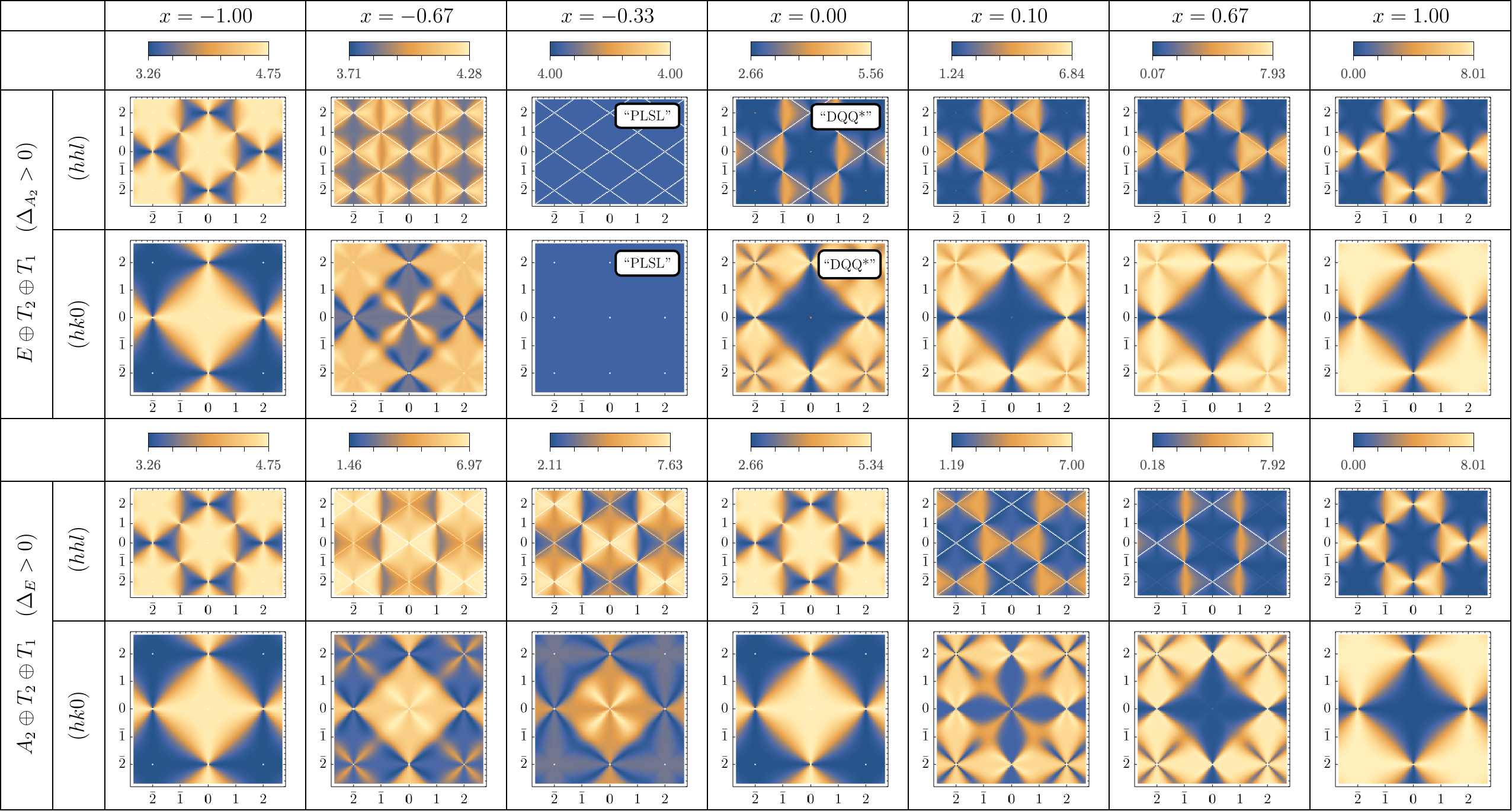
Figure 9: Evolution of the zero-temperature SCGA structure factors (Appendix D), computed from the projector to the flat bands, for two of the four 3-fold degenerate lines—$E\oplus T_{2}\oplus T_{1}$ (top two rows) and $A_{2}\oplus T_{2}\oplus T_{1}$ (bottom two rows)—in the cubic $(hk0)$ and $(hhl)$ planes of reciprocal space. At the right end is the structure factor for the HAFM, while at the left end is the structure factor of the HAFM${}_{\text{dual}}$, while the middle column is the $J_{z\pm}=0$ case. All cases show flat lines along $(hhh)$, visible in the $(hhl)$ plane, and fourfold pinch points, visible in the $(hk0)$ plane. Note that the color scale starts from the minimum intensity and goes to the maximum intensity of the flat band; higher intensities from the singular band touchings lines and points appear white. The $\Delta_{A_{2}}>0$ triple line was first discussed in Ref. [45], but only one point on the line—the “pinch-line spin liquid” (PLSL), corresponding to $J_{3}<0$ and all other couplings zero—was studied. The $J_{z\pm}=0$ point on this triple line is the $J_{\pm\pm}$-dual (denoted with an asterisk) of the “DQQ” model from Ref. [47]. The $\Delta_{E}>0$ triple line was recently studied in detail in Ref. [44].

There are a few possible scenarios which can then in principle distinguish:

1. The intersection is zero-dimensional, $\dim\mathscr{G}=0$. Then $\mathscr{G}$ is a discrete space, and at each point in $\mathscr{G}$ the Hessian is positive-definite. A generic spin configuration is orthogonal to $\mathscr{F}$. We can distinguish the following cases

   1. The number of discrete ground states, $|\pi_{0}(\mathscr{G})|$, is of order one. The system orders.

   2. The ground state entropy is subextensive, such that $\log|\pi_{0}(\mathscr{G})|\propto L^{k}$ with $0<k<3$. The system may potentially undergo dimensional reduction without ordering [55].

   3. The ground state entropy is extensive, such that $\log|\pi_{0}(\mathscr{G})|\propto L^{3}$. We further differentiate:

      1. The ground state is a trivial paramagnet;

      2. the ground state is a symmetry-broken [102, 103] or fragmented [104, 105] spin liquid;

      3. the ground state is a symmetric spin liquid, as in the $T_{1,\text{ice}}$ region of the pyrochlore phase diagram.

2. The intersection is sub-extensive, i.e. $\cramped{\dim\mathscr{G}\propto L^{k}}$ with $\cramped{0<k<3}$. Then $\mathscr{G}$ is parameterized locally by a subextensive number of continuous compact parameters. It may have one or more connected components. A generic spin configuration has a sub-extensive projection into $\mathscr{F}$.

3. The intersection is extensive, $\dim\mathscr{G}\propto L^{3}$, and is parameterized locally by an extensive number of parameters. It may have one or more connected components. A generic spin configuration has non-zero overlap with $\mathscr{F}$ of order $(\dim\mathscr{G})/L^{3}$. We can further distinguish the following possibilities:

   1. The system exhibits symmetry breaking, either

      1. order-by-singularity selects a ground state;

      2. order-by-disorder selects a ground state;

      3. nematic but liquid-like order [43, 44].

   2. The system exhibits no symmetry breaking, either

      1. a liquid-to-liquid crossover [47];

      2. the ground state is a fully symmetric spin liquid, e.g. the pyrochlore HAFM [26, 28].

Case 1(a) is likely a common occurrence whenever the number of flat bands is less than a third of the total number of bands, following the rule of thumb. Case 1(b) and case 2 both imply there is an obstruction to consistently “gluing together” single-tetrahedron ground states in a corner-sharing fashion to build ground states of the entire system, i.e. what Ref. [55] calls the “Lego-brick” construction. In case 2 $\mathscr{G}$ is connected, but we expect that the subextensive dimension will result in either order-by-singularity or order-by-disorder ground state selection. Unfortunately we do not known any explicit examples where this case occurs. Lastly, case 3(a) has an extensive ground state manifold yet a symmetry broken ground state is selected. We are not aware of examples of possibilities (i) or (ii), but believe one of these may occur on the $\Delta_{E}>0$ line, where Ref. [44] recently reported selection of the $A_{2}$ all-in-all-out configurations when $J_{z\pm}$ is small, we discuss this further in Section VI.3.1.

If the system avoids these ordering mechanisms, this leaves cases 1(c) and 3(b). Case 1(c)(i), a trivial paramagnetic ground state, can occur for example in a Potts model with a large number of states, where the system is trivially disordered to zero temperature. Case 1(c)(ii) means that the system exhibits an extensive but unsaturated ordered moment, while continuing to fluctuate as a spin liquid to zero temperature. Case 3(b)(i) was recently reported in Ref. [47] which we discuss briefly in the next section. Finally, cases 1(c)(iii) and 3(b)(ii) correspond to discrete and continuous symmetric spin liquids, respectively, many examples of which are known.

VI.2 Identified Pyrochlore Spin Liquids

Previous studies have looked at a variety of spin liquid models on the pyrochlore lattice emerging at the triple-intersection of phases. The earliest recognized was the HAFM, which has long been a canonical example of a classical spin liquid [26, 72, 73, 74, 27, 75, 28]. Referring to the first row of Table 6, it has six flat bands with three quadratically dispersing bands touching at $\bm{q}=\bm{0}$. At low temperature each tetrahedron is constrained to have zero net spin, i.e. $T_{1\parallel}$ is gapped (c.f. Eq. 60). The low-temperature $T\to 0^{+}$ spin-spin correlations ($T$ being temperature) $\langle S_{i}S_{j}\rangle$ are $1/r^{3}$ power-law decaying [27, 28]. Their Fourier transform, the spin structure factor,

$$S(\bm{q})=\frac{1}{L^{3}}\sum_{i,j}\langle S_{i}S_{j}\rangle e^{-i\bm{q}\cdot(\bm{r}_{j}-\bm{r}_{i})},$$ (73)

exhibits characteristic “pinch-point” correlations, i.e. a diffusive profile with bow-tie singularities located at zone centers due to the long-range correlations arising from a local constraint [27, 28, 75]. The HAFM structure factor is shown in the right-most column of Fig. 9. As we have discussed throughout this paper, there is an additional HAFM${}_{\text{dual}}$model with negative $J_{z\pm}$, whose physics is exactly the same and whose ground states are in bijection with those of the HAFM by a $\pi$ rotation about the local easy axis. The corresponding structure factor is shown in the left-most column of Fig. 9.

In 2016 another model was found, the “pinch line spin liquid” (PLSL) [45], which was identified with the model $J_{3}<0$ and $J_{1}=J_{2}=J_{4}=0$ in terms of the global basis parameters in Eq. 3. Ref. [45] discussed this model as a particular example of a family of models characterized by gapping $A_{2}$ and $T_{1+}$, i.e. the $\Delta_{A_{2}}>0$ line in Footnote 13, though the authors did not parameterize the entirely family. The interest in this model was that it exhibits pinch line singularities rather than pinch points, i.e. singular correlations everywhere along the high-symmetry $(hhh)$ line in reciprocal space. It corresponds to the second row of Table 6, hosting four flat bands and a singe flat line along the high-symmetry $(hhh)$ lines in reciprocal space plus three quadratically dispersing bands at the zone center. From the rest of the table it is clear that pinch lines are actually not unique to this model or this triple line—indeed they appear at all the triple intersections.

In 2017 the “pseduo”-HAFM (pHAFM) point was pointed out in Ref. [43], which is just the HAFM in the local basis, i.e. $J_{\pm}=-J_{zz}/2$, $J_{zz}>0$, and $J_{\pm\pm}=J_{z\pm}=0$. The physics of this model is identical to the HAFM, since they are mapped to each other by a local on-site mapping of each spin from its local frame to the global frame. We have marked this in Footnote 13, it is the isolated triple point occurring on the $T_{2}\oplus T_{1}$ phase boundary where it is pierced by the line of $T_{1}$ degeneracy. It has degenerate irreps $T_{2}\oplus T_{1,\text{ice}}\oplus T_{1,\text{planar}}$ in Table 6. Ref. [43] also studied the $T_{2}\oplus T_{1,\text{planar}}$ line, i.e. the intersection of the $T_{1}\oplus T_{2}$ phase boundary and the $J_{z\pm}=0$ plane, and found the system exhibits a finite-temperature spin liquid regime with a phase transition to nematic phase at low temperature with broken rotational symmetry.

In 2020 another non-trivial spin liquid was then found, the so-called “rank-2 U(1)” spin liquid [46]. This was inspired by a surge of interest in gauge theories with a symmetric rank-2 tensor electric fields, which are prototypical fractonic theories [106, 107, 108, 109] whose excitations have highly constrained mobility due to local conservation of dipole and quadrupole moments. Ref. [45] first showed how to organize the irreps into a tensor, and Ref. [46] exploited this structure by recognizing that a low-energy symmetric trace-free tensor field could be obtained by gapping the $A_{2}$ (trace component) and $T_{2}$ (anti-symmetric components) on each tetrahedron, along the with the vector $T_{1\parallel}$. This leaves only $T_{1\perp}\oplus E$ in the ground state, which together form the desired symmetric trace-free tensor on each tetrahedron. This occurs along a one-dimensional locus in the $T_{1}\oplus E$ phase boundary along which $J_{3}=0$, so that the decoupled $T_{1}$ irreps are $T_{1,\text{ice}}$ and $T_{1,\text{planar}}$. This line is precisely traced by restricting the Hamiltonian Eq. 4 to only Heisenberg and DM interactions, which is shown in Fig. 7 by the green circle (the inset shows how this family runs long the $T_{1}\oplus E$ phase boundary). However, just being on this phase boundary is insufficient degeneracy for flat bands (c.f Table 6), and the system selects the $E$ phase ground states [57]. Ref. [46] attempted to remedy this ordering by introducing breathing anisotropy to relax some of the constraints on a subset of tetrahedra. The rank-2 U(1) spin liquid is then obtained at finite temperatures, though the system still orders at sufficiently low temperature [110].

In 2023 Ref. [47] studied another spin liquid, which was called the “dipolar-quadrupolar-quadrupolar” (“DQQ”) model. This is the second isolated triple point other than the pHAFM, sitting at the intersection of the $T_{1}\oplus E$ phase boundary and the $T_{1}$-degenerate line in Footnote 13, i.e. with degenerate irreps $E\oplus T_{1,\text{ice}}\oplus T_{1,\text{planar}}$ in Table 6. This model was found to exhibit a classical liquid-to-liquid crossover, where the spin ice states are entropically selected from the ground state manifold at very low temperatures. It also has a $J_{\pm\pm}$-dual model, which is the point on the $\Delta_{A_{2}}>0$ line at $J_{z\pm}=0$.

Recently, Ref. [44] studied the line with $\Delta_{E}>0$, and found that for small $J_{z\pm}$ it exhibits a ground state selection of $A_{2}$ order, while for larger $J_{z\pm}$ (closer to the HAFM) it exhibits a nematic ordering similar to that on the $\cramped{T_{2}\oplus T_{1,\text{planar}}}$ line. It was also reported that the nematic symmetry breaking occurs ubiquitously on the $T_{1}\oplus T_{2}$ phase boundary, which may be a consequence of flat planes (rather than flat bands), c.f. Table 6.

Finally, Ref. [111], which appears concurrently with this work, performed an exhaustive search of all degenerate combinations of irreps and determined the corresponding Gauss laws and stability for pyrochlore spin liquids. They identify the HAFM${}_{\text{dual}}$  model and show that the $\Delta_{A_{2}}>0$ line is a stable spin liquid family, but otherwise have found that there are no additional stable classical spin liquids with nearest-neighbor interactions.

Before moving on, we note that further-neighbor interactions can stabilize entirely novel spin liquids, in particular the author has shown in Ref. [102] the existence of a 2-form U(1) classical spin liquid with Ising spins on the pyrochlore lattice, by generalizing the zero-divergence constraint of spin ice to a zero-curl constraint. Its isotropic extension generalizes the HAFM spin liquid, and the possibility of anisotropic generalization of 2-form U(1) spin liquids remains an open possibility.

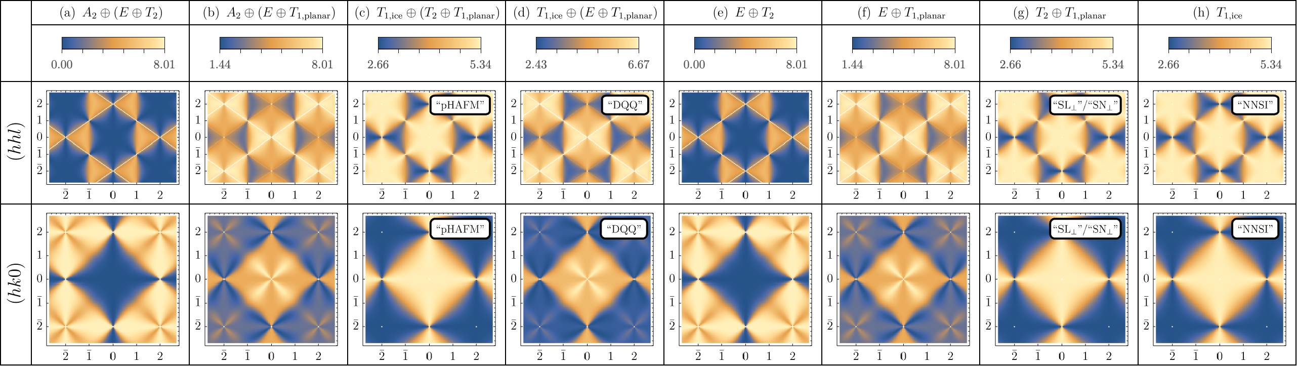
Figure 10: Spin structure factor for flat band cases not on the two lines shown in Fig. 9. (a) On the $\Delta_{T_{-}}>0$ line there are two flat bands with pinch line singularities. Because the ground state does not involve a $T_{1}$ irrep, the ground state physics is independent of position along this line, and the structure factor does not evolve along it. (b) The $\Delta_{T_{2}}>0$ line does not have flat bands (only flat planes) except when $J_{z\pm}=0$. Note that in both cases (a) and (b) the $A_{2}$ phase is accidentally degenerate and does not contribute to the flat bands. (c) The isolated pseudo-HAFM triple point [43] contains decoupled contributions from $T_{1,\text{ice}}$ and the planar $T_{1}$ and $T_{2}$ irreps. (d) The isolated “DQQ” triple point [47] contains decoupled contributions from the $T_{1,\text{ice}}$ and the planar $T_{1}$ and $E$ irreps. (e) The planar $E$ and $T_{2}$ irreps combine to form non-trivial flat bands on this phase boundary. (f) The planar $E$ and $T_{1}$ irreps combine to form non-trivial flat bands on this phase boundary in the $J_{z\pm}=0$ plane. (g) The planar $T_{2}$ and $T_{1}$ irreps combine to form non-trivial flat bands on this phase boundary in the $J_{z\pm}=0$ plane. This region was studied in Ref. [43] and found to be a nematic spin liquid. (h) The structure factor in the nearest-neighbor spin ice (NNSI) region of the $T_{1}$ phase. Note that (a) is equivalent to (e) plus extra intensity at zone center due to the extra decoupled $A_{2}$ irrep; (b) is equivalent to (f) for the same reason; (c) is equivalent to (g) plus (h); and (d) is equivalent to (f) plus (h).

Table 4: Flat degeneracies within each phase (c.f. Fig. 2). For the $T_{1}$ phase additional degeneracies occur when $J_{z\pm}=0$. $T_{2}$ and $T_{1,\text{planar}}$ have flat lines along the $(hhh)$ directions, while $T_{1,\text{ice}}$ hosts two flat bands corresponding to the spin ice ground states. Note that the sum of numbers in each row equals the dimension of the irrep in the first column—the number of zero modes at the $\Gamma$ ($\bm{q}=\bm{0}$) point.

Table 5: Flat degeneracies on the phase boundaries. Rows highlighted in gray indicate that the flat degeneracies are more than the sum of parts in Table 6. The $E\oplus T_{2}$ boundary carries two flat bands, while the $E\oplus T_{1}$ and $T_{2}\oplus T_{1}$ phase boundaries carry non-trivial flat bands when $T_{1}=T_{1,\text{planar}}$.

Table 6: Flat band degeneracies on the triply-degenerate cases listed in Table 3 and depicted in Footnote 13. The HAFM points have the highest degeneracy, which is partially lifted along the four triply-degenerate lines. Note that flat $\{hhl\}$ planes imply a triple $(hhh)$ line intersection, indicated with square brackets. Note that combining easy-axis with easy-plane irreps always results in a trivial stacking of degeneracies, indicated with parentheses on non-highlighted lines.

VI.3 Catalog of Pyrochlore Flat Bands

With the full structure of the phase diagram now plainly exposed in Footnote 13, we can systematically account for all possible degenerate combinations of irreps, how they relate to each other in the phase diagram, and how they generate flat bands. Starting with the triple lines, these can be parameterized by a single parameter $x\in[-1,1]$, such that

$$\operatorname{sign}(J_{z\pm})=\operatorname{sign}(x)\quad\text{and}\quad\frac{\Delta_{I^{\prime}}}{\Delta_{T_{1+}}}=\max\left(\frac{\Delta_{I^{\prime}}}{\Delta_{T_{1+}}}\right)(1-|x|),$$ (74)

where the maximum is given by the right hand side of the inequalities in Table 3. Note that for $I^{\prime}=T_{1-}$ the line is parameterized in Table 3 according to the splitting of the $T_{1}$ energies, but for the $\Delta_{T_{1-}}\geq 0$ portion it can be parameterized as in Eq. 74 with $0\leq\Delta_{T_{1-}}/\Delta_{T_{1+}}\leq 1/2$. For all four lines this parameterization yields the HAFM at $x=1$ and the HAFM${}_{\text{dual}}$ at $x=-1$. The flat band degeneracies on these lines are listed in Table 6.

For each of the lines we have computed the zero-temperature spin structure factor, Eq. 73, in the self-consistent Gaussian approximation (SCGA) [112, 113, 75] in the limit of zero temperature, which is proportional to the projector $P_{\mathscr{F}}$ to the flat band subspace (c.f. Appendix D),

$$S(\bm{q})_{T\to 0^{+}}=\frac{n_{\text{tot}}}{3n_{\text{flat}}}\sum_{\mu,\nu}\sum_{\alpha}[P_{\mathscr{F}}(\bm{q})]_{\mu\nu}^{\alpha\alpha}\quad(\text{SCGA}).$$ (75)

The touching of the dispersive bands with the flat bands give rise to characteristic pinch singularities in these structure factors. Figure 9 shows the evolution of the structure factor along the $\Delta_{A_{2}}>0$ and $\Delta_{E}>0$ lines, both exhibiting a combination of pinch lines and pinch points. The triple line with $\cramped{\Delta_{T_{1-}}>0}$ has no dependence on the canting angle because both $T_{1}$ irreps are gapped along this line, meaning that the structure factor is the same everywhere on this line, shown in Fig. 10(a). The last triple line, with $\Delta_{T_{2}}>0$ has no flat bands, only flat planes, except when $\cramped{J_{z\pm}=0}$, shown in Fig. 10(b). The remaining two triple points, the pHAFM and “DQQ” models, are shown in Fig. 10(c,d). Various phase boundaries also exhibit flat band degeneracies, which are shown in Fig. 10(e,f,g). Lastly, the structure factors for spin ice, i.e. the $T_{1,\text{ice}}$ ground state, are shown in Fig. 10(h).

VI.3.1 Trivially Stacked Band Touchings and Easy-Axis Selection

Simply tuning additional irreps to be degenerate does not necessarily enhance the flat band degeneracies, meaning that the long-wavelength band structure at these points is just a trivial “stacking” of the band structure of the separate irreps, i.e. an accidental degeneracy. We should therefore ask which combinations of irreps enhance the degeneracies beyond the individual components. Another way to state this is, there is a topological invariant associated to how the normalized eigenvectors of the interaction matrix wind around the reciprocal space loci where flat bands touch dispersive bands [49, 50]; when we add additional band touching degeneracies, does the topological invariant change? For this reason we also provide the degeneracies within each phase in Table 6 and on each phase boundary in Table 6.

Checking the cases in Table 6 containing $T_{1,\text{ice}}$ and comparing to the corresponding degeneracies in Table 6 shows that the three boundaries between the $J_{z\pm}=0$ $T_{1,\text{ice}}$ region of the neighboring phases (c.f. Fig. 5(b)) do not obtain any additional flat degeneracies beyond those $T_{1,\text{ice}}$ and the neighboring phase. This is because in the $J_{z\pm}=0$ plane the $T_{1,\text{ice}}$ irrep contains only the easy-axis spin components, while the ground state irreps of the surrounding phases contain only the easy-plane spin components. Thus tuning to these phase boundaries simply “stacks” the degeneracies of the two sides, as the irreps are decoupled when $J_{z\pm}=0$.

The same applies for combining the easy-axis $A_{2}$ irrep with any easy-plane irreps. For example, the $\cramped{A_{2}\oplus E\oplus T_{2}}$ line in Table 6 has the same flat degeneracies of the $\cramped{E\oplus T_{2}}$ phase boundary in Table 6 plus one extra zone-center quadratic band touching coming from the $A_{2}$ irrep. Correspondingly, the SCGA structure factor for this line shown in Fig. 10(a) is exactly the SCGA structure factor of the $E\oplus T_{2}$ phase boundary in Fig. 10(e) plus some extra zone-center intensity from the $A_{2}$ degeneracy (not visible in the figure). The same occurs for the $\cramped{A_{2}\oplus E\oplus T_{1,\text{planar}}}$ combination in Fig. 10(b) compared to the $\cramped{E\oplus T_{1,\text{planar}}}$ combination in Fig. 10(f). Similarly, the two combinations with $T_{1,\text{ice}}$, (b) and (c), are equivalent to adding the same combination without $T_{1,\text{ice}}$, (g) and (f) respectively, with the $T_{1,\text{ice}}$ structure factor in (h).

Such trivial stacking does not necessarily rule out interesting physics arising due to the enhanced degeneracy. For example, the $E\oplus T_{1,\text{planar}}\oplus T_{1,\text{ice}}$ triple point was studied in detail in Ref. [47] (dubbed the “DQQ” model), and exhibits a finite-temperature liquid-to-liquid crossover. At finite temperature it develops correlations matching the SCGA, while at very low temperature it selects the spin ice manifold and remains a spin liquid. The reason is because the degeneracy with the easy-plane configurations implies that if the spins are aligned along the easy axis their transverse fluctuations is greatly enhanced, meaning that the Hessian about the easy-axis configurations should will contain gapless modes easy-plane modes on each tetrahedron. The Hessian for a spin ice state has an extensive number of zero modes, while for a generic ground state it does not [47]. We believe that this mechanism should be universal: selection of the easy-axis configurations will be preferred for all cases in which the ground state irreps split into decoupled easy-axis and easy-plane components. From Eq. 69 it clear that if $\tilde{\bm{z}}_{i}$ are along the easy-axis then the Hessian will inherit all of the zero-energy easy-plane normal modes of the interaction matrix. In particular, this implies that cases that are trivially stacked with $A_{2}$ will select the all-in-all-out ground state, an example of order-by-singularity. In this sense, the liquid-to-liquid crossover of the DQQ model studied in Ref. [47] is an example of a selection of the ice manifold due to singularities in the ground state manifold, a “easy-axis-spin-liquid-by-singularity”.

VI.3.2 Intertwined Flat Bands

On the other hand, combinations of two easy-plane irreps always yields an enhanced degeneracy, highlighted gray in Table 6. For example, $T_{2}\oplus T_{1,\text{planar}}$ has four flat bands despite neither the $T_{2}$ phase nor the $T_{1,\text{planar}}$ region of the $T_{1}$ phase having any flat bands. Such cases exhibit “intertwined” flat bands which are more than the sum of their parts, meaning that the topological invariant arising from the winding of the eigenvectors of the interaction matrix around the degenerate points in reciprocal space changes. Alternatively, the band representation with degeneracy does not trivially decompose into a sum of the components [51]. This will result in additional degeneracies away from the zone center as well. The complete list of phase boundaries with intertwined flat bands are precisely the three combination of the easy-plane ground states: $E\oplus T_{2}$, $E\oplus T_{1,\text{planar}}$, and $T_{2}\oplus T_{1,\text{planar}}$. The three boundaries of the $T_{1}$ phase generically contain intertwined but subextensive flat bands: $A_{2}\oplus T_{1}$ and $E\oplus T_{1}$ have intertwined flat lines while $T_{2}\oplus T_{1}$ has intertwined flat planes. Finally, moving to the triple lines and points in Table 6, the $\Delta_{T_{1-}}>0$ has no intrinsically new flat bands, it is a trivial stacking of the $E\oplus T_{2}$ phase boundary flat bands with the $A_{2}$ irrep. The $\Delta_{T_{2}}>0$ triple line has no flat bands but has intertwined flat planes. The remaining two triple lines, $\Delta_{A_{2}}>0$ and $\Delta_{E}>0$, both have intertwined flat bands, and the HAFM points have intertwined flat bands.

VI.4 Charge-Flux Intertwinement of Irreps, Band Touchings, and Gauss Laws

As we have now seen in detail, various degenerate combinations of irreps yield spin liquids, but not all combinations are possible. Here we provide some further insight into how the various irreps are interrelated to each other in various spin liquids, some acting as fluxes and others acting as charges of an emergent gauge theory. The Hamiltonian can be expressed as

$$H=\sum_{t}\sum_{I,a}J_{I}|({\bm{m}}_{I}^{a})_{t}|^{2},$$ (76)

where $t$ indexes the tetrahedra. For various fine-tuned degeneracies tabulated in Tables 6, 6 and 6 various flat bands appear, some of which support classical spin liquids. For each of the flat cases there is a quadratic band touching with the flat bands which determines an emergent Gauss law for the coarse-grained description of the system in terms of gauge fluxes [28, 49, 50]. As we have seen, we cannot tune arbitrary irreps to be degenerate, some possibilities like $A_{2}\oplus T_{1,\text{ice}}$ are not possible. While the irreducible representation analysis decouples the spin components into seemingly independent degrees of freedom, there is a non-trivial relation between the different irrep components.

VI.4.1 Easy-Axis Irreps

Consider first the limit of the pure-$J_{zz}$ Hamiltonian with all other couplings zero. This corresponds to the maximally anisotropic limit where all spins lie along their easy-axes, with corresponding irrep decomposition $A_{2}\oplus T_{1,\text{ice}}$. All other irreps, corresponding to easy-plane modes, do not appear in the Hamiltonian, their energies are $J_{I}=0$. Those absent easy-plane irreps cannot be the ground state, therefore we must have that $J_{A_{2}}<0$ and $J_{T_{1,\text{ice}}}>0$ or vice-versa, e.g. if $A_{2}$ is gapped then $T_{1,\text{ice}}$ must be the ground state. To see how these irreps are coupled, it is instructive to write the Hamiltonian in this limit in terms of the pyrochlore adjacency matrix,

$$H_{J_{zz}} =\frac{J_{zz}}{2}\sum_{ij}A_{ij}S_{i}^{z}S_{j}^{z}\quad(\text{local $z$})$$

$$=\text{const.}+J_{A_{2}}\sum_{t}|m_{A_{2}}|^{2},$$ (77)

where $A_{ij}=+1$ if $i$ and $j$ are nearest-neighbor sites and zero otherwise. On a single tetrahedron, this has the form

$$A_{ij}=\begin{pmatrix}0&1&1&1\\ 1&0&1&1\\ 1&1&0&1\\ 1&1&1&0\end{pmatrix}\quad(i,j\in t),$$ (78)

which has a single eigenvalue $+3$ corresponding to the $A_{2}$ irrep and a triply degenerate eigenvalue $-1$ corresponding to the $T_{1,\text{ice}}$ irrep, whose associated eigenvectors are

$$A_{2}: \qquad(+1,+1,+1,+1)$$ (79)

$$T_{1,\text{ice}}: \quad\begin{cases}(+1,+1,-1,-1)\\ (+1,-1,+1,-1)\\ (-1,+1,+1,-1)\end{cases}$$ (80)

Notice that the three $T_{1,\text{ice}}$ eigenvectors differ from the $A_{2}$ eigenvector by reversing two spins. Correspondingly the $A_{2}$ ground states are all-in-all-out, Fig. 11(b), while the $T_{1,\text{ice}}$ ground states are 2-in-2-out, Fig. 11(a). At the lattice level the 2-in-2-out states have “zero divergence” if we think of $S_{i}^{z}$ as carrying a flux in or out of the tetrahedron, while the all-in-all-out states have maximal divergence. Thus if we associate the $T_{1,\text{ice}}$ eigenmodes to zero-divergence fluxes, the $A_{2}$ eigenmode is the corresponding charge which sources a non-zero divergence. Another way to see this is that there is a sum rule relating these irreps,

$$|m_{A_{2}}|^{2}+|\bm{m}_{T_{1,\text{ice}}}|^{2}=\sum_{i}(S_{i}^{z})^{2}.$$ (81)

If all spins lie along the easy axis in the ground state then the right hand side is a positive constant and either the $A_{2}$ or $T_{1,\text{ice}}$ is maximized, implying the other is minimized. Notably this implies that it is not possible to have both $T_{1,\text{ice}}$ and $A_{2}$ degenerate in the ground state, because raising the energy of one lowers the energy of the other and vice-versa. We see this in Footnote 13, and also in the fact that the last triple combination in Table 3 has no solution.

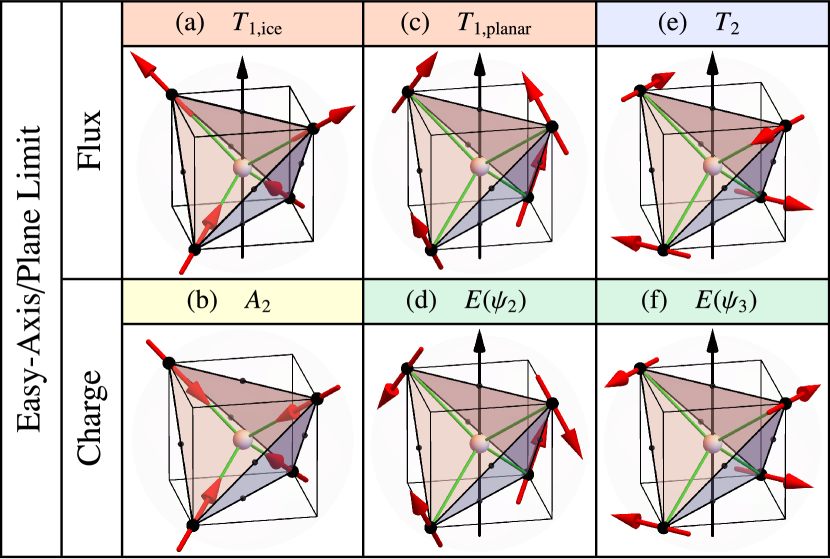
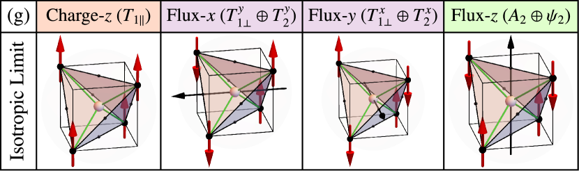
\begin{overpic}[width=433.62pt]{dispersion.pdf} \put(1.0,45.0){Charge $Q$} \put(1.0,17.0){Flux $\bm{B}$} \put(63.0,42.0){$Q(\bm{q})$} \put(61.0,18.0){$\hat{\bm{q}}\cdot\bm{B}$} \put(57.0,4.0){$\hat{\bm{q}}\times\bm{B}$} \put(43.0,34.0){coupled} \put(42.0,30.0){tetrahedra} \put(9.0,0.0){$q_{x}$} \put(37.0,5.0){$q_{y}$} \put(73.0,0.0){$q_{x}$} \put(95.0,5.0){$q_{y}$} \put(20.0,-5.0){(h)} \put(77.0,-5.0){(i)} \end{overpic}

Figure 11: Illustration of the flux-charge relation between irreps. Each 3-component vector irrep acts as a flux, and its corresponding charge is obtained by reversing two spins. In the long-wavelength limit, gapping one of the charges will force the corresponding flux to have zero divergence. (a-f) In the easy-axis/easy-plane limit $J_{z\pm}=J_{\pm\pm}=0$, the local $x,y,z$ components are decoupled into three independent charge-flux combinations: (a,b) The $T_{1,\text{ice}}$ irrep correspond to 2-in-2-out states with zero lattice divergence, while the $A_{2}$ irrep corresponds to all-in-all-out states with maximal lattice divergence [27, 75, 74]; (c,d) Flipping two spins from the $T_{1,\text{planar}}$ irrep results in the a $\psi_{2}$ configurationl; (e,f) Flipping two spins from a $T_{2}$ configuration results in a $\psi_{3}$ configuration. (g) In the isotropic limit the global $x,y,z$ components decouple, the three $\smash{\smash{T_{1\parallel}}}$ irrep components $\mathcal{M}$ act as the charges, and the fluxes correspond to the columns of $\mathcal{B}$. (h,i) Illustration of how gapping the charges yields a zero-divergence constraint on the fluxes at the level of bands. (h) In the limit where the $A$ tetrahedra are decoupled (zero coupling on the $B$ tetrahedra) the irreps label a set of flat bands, one for the charge and three for the flux, shown on the left. (i) Turning on the coupling between tetrahedra, the necessity that the charge is zero on the $B$ tetrahedra restricts the allowed configurations on the surrounding $A$ tetrahedra, resulting in the longitudinal (along $\hat{\bm{q}}$) component of the coarse-grained flux becoming dispersive. The transverse (orthogonal to $\hat{\bm{q}}$) components remain flat.

VI.4.2 Long-Wavelength Gauss Law

This flux-charge intertwinement has a dramatic consequence in the long-wavelength expansion of the Hamiltonian: the band structure of $\mathscr{J}$ has a single and triple degeneracy at the zone center corresponding to the $\bm{q}=\bm{0}$ single-tetrahedron irrep eigenmodes, while away from the zone center the bands disperse. Fourier transforming the single-tetrahedron modes, which vary from tetrahedron to tetrahedron, we can perform a long-wavelength expansion of the Hamiltonian in which the single-tetrahedron modes become coarse-grained fields—$A_{2}$ becomes a scalar field and $T_{1,\text{ice}}$ a vector field $\bm{B}$—and we find that forcing the $A_{2}$ to be zero (taking $J_{zz}>0$ and going to low temperature) forces the divergence of $\bm{B}$ to be zero [74, 75, 28]. In the $T_{1,\text{ice}}$ ground state the coarse-grained Gauss law can then be simply read off,

$$\bm{q}\cdot\bm{B}_{T_{1,\text{ice}}}(\bm{q})=0\quad\Leftrightarrow\quad\nabla\cdot\bm{B}_{T_{1,\text{ice}}}=0.$$ (82)

One way to rationalize this is to consider the fact that the pyrochlore lattice can be divided into two sets of tetrahedra, “$A$” and “$B$”, such that an $A$ tetrahedron is surrounded by four $B$ tetrahedra and vice-versa. If we turn off the couplings on the $B$ tetrahedra then the bands of the interaction matrix would be dispersionless (flat) with degeneracies determined by the single-tetrahedron irreps, Fig. 11(h), corresponding to completely decoupled $A$ tetrahedra which only have to satisfy their local constraint but can be in arbitrary ground states. Turning on the $B$ tetrahedra couplings, we realize that we cannot choose the $A$ tetrahedra ground states arbitrarily, because we have to ensure that the $B$ tetrahedra are also in a ground state, thus some of the flat bands from the decoupled limit become dispersive, Fig. 11(i), with a band touching that remains at the zone center. This band touching then determines the emergent Gauss law for the fluxes when the corresponding charges are gapped: the longitudinal component of the field is suppressed, while its transverse modes remain free to fluctuate.

On the other hand, if instead the flux irrep is gapped then the constraint on the scalar charge must be a zero-gradient constraint. For example, taking $J_{zz}<0$ in in the $A_{2}$ phase the long-wavelength expansion can only yield $|\bm{q}|^{2}m_{A_{2}}^{2}$, the bottom band of the interaction matrix disperses upwards, and the coarse-grained constraint is $\nabla m_{A_{2}}=0$.

VI.4.3 Easy-Plane Irreps

We can extend this relation to the other irreps. First, consider adding the easy-plane components without anisotropies, i.e. $J_{\pm\pm}=J_{z\pm}=0$. The easy-plane irreps are $E$, $T_{2}$, and $T_{1,\text{planar}}$, with Hamiltonian

$$H_{J_{\pm}} =-J_{\pm}\sum_{ij}A_{ij}(S_{i}^{x}S_{j}^{x}+S_{i}^{y}S_{j}^{y})\quad(\text{local $x,y$}),$$

$$=\text{const}.-J_{E}\sum_{t}|\bm{m}_{E}|^{2}.$$ (83)

It follows from the first line that the local $x$ and $y$ modes are decoupled, and the corresponding eigenvectors are again given by Eq. 80. It then follows from the local $x$ components that the $T_{1,\text{planar}}$ modes are fluxes with the $\psi_{2}$ the corresponding charges, while from the local $y$ components it follows that the $T_{2}$ modes are fluxes with $\psi_{3}$ the corresponding charges, as illustrated in Fig. 11(c-f). Raising the energy of one of the charge irreps lowers the energy of the corresponding flux, which should satisfy a zero-divergence condition in the long-wavelength coarse-grained limit, owing to the sum rule

$$|\bm{m}_{E}|^{2}+|\bm{m}_{T_{2}}|^{2}+|\bm{m}_{T_{1,\text{planar}}}|^{2}=\sum_{i}[(S_{i}^{x})^{2}+(S_{i}^{y})^{2}].$$ (84)

Due to the symmetry of the lattice we cannot split the energy of the $\psi_{2}$ and $\psi_{3}$ charges since they are two components of a single irreducible representation. For $J_{\pm}<0$ then ground state is a combination of $T_{1,\text{planar}}$ and $T_{2}$ fluxes, which must both satisfy a zero-divergence constraint in the long-wavelength limit [43],

$$\bm{q}\cdot\bm{B}_{T_{1,\text{planar}}}(\bm{q})=\bm{q}\cdot\bm{B}_{T_{2}}(\bm{q})=0.$$ (85)

This suggests the ground state behaves as two decoupled copies of a Coulomb phase, though Ref. [43] found that it exhibits nematic symmetry breaking. For $J_{\pm}>0$ the $E$ ground state is selected, a “charge condensate” of the $\psi_{2}$ and $\psi_{3}$ irreps, one of which is chosen via order by disorder [53, 54, 25, 90].

VI.4.4 Easy-Axis Plus Easy-Plane

Combining the analysis for the pure-$J_{zz}$ and pure-$J_{\pm}$, we note that the fine-tuned point when $J_{zz}=-2J_{\pm}>0$ corresponds to the isolated $T_{1,\text{ice}}\oplus T_{1,\text{planar}}\oplus T_{2}$ triple point, where the ground state is described by three Gauss laws, Eqs. 82 and 85, which is precisely the pHAFM. The Hamiltonian can be expressed using the three-component diagonal components of the multipole tensor defined in Eq. 27c, as

$$H=J_{E/A_{2}}\sum_{t}|\bm{\mathcal{Q}}_{t}|^{2},$$ (86)

where $J_{E}=J_{A_{2}}$ at this point. For $J_{E/A_{2}}>0$ the ground state is described by three decoupled Coulomb phases. For $J_{E/A_{2}}<0$ the ground state becomes the pseduo-ferromagnet (pHFM), which is a special point on the $A_{2}\oplus E$ phase boundary with a global SO(3) symmetry, see Section VII.

On the other hand there is the $A_{2}\oplus T_{2}\oplus T_{1,\text{planar}}$ triple point when $J_{zz}<0$. However, as discussed in Section VI.3.1 this will not yield a more complicated Gauss law, instead it just adds the constraint $\nabla m_{A_{2}}=0$. This is one example of a trivially stacked band degeneracy. The result is that the $T_{2}\oplus T_{1,\text{planar}}$ and $A_{2}$ behaviors compete, and in this case the easy-axis order winds [44].

VI.4.5 Isotropic Limit

Next consider the isotropic case, i.e. the Heisenberg model, which we can write as a sum of three (classically) decoupled Hamiltonians

$$H_{J_{\text{Heis}}} =\frac{J_{\text{Heis}}}{2}\!\!\sum_{\alpha\in\{x,y,z\}}\left(\sum_{ij}A_{ij}S_{i}^{\alpha}S_{j}^{\alpha}\right)\quad(\text{global $x,y,z$}),$$

$$=\text{const.}+J_{\smash{T_{1\parallel}}}\sum_{t}|\bm{\mathcal{M}}_{t}|^{2},$$ (87)

where $\bm{\mathcal{M}}$ was defined in Eq. 27a. We can immediately infer that the three charges are the three components of the net-moment $\smash{T_{1\parallel}}$ irrep. The $z$-component is shown in Fig. 11(g), along with the three flux components obtained by reversing two spins. The flux components precisely corresponding to the last column of the multipole tensor $\bm{\mathcal{B}}$, Eq. 27b. Each column of the tensor corresponds to a flux vector, and indeed these are precisely the coarse-grained fluxes which were defined in Refs. [74, 75], and we can define $\bm{\mathcal{B}}\equiv(\bm{B}_{x},\bm{B}_{y},\bm{B}_{z})$. Each of these fluxes satisfies a coarse-grained zero-divergence constraint at low temperature when $J_{\text{Heis}}>0$,

$$\bm{q}\cdot\bm{B}_{\alpha}(\bm{q})=0.$$ (88)

This can also be expressed as a single tensor Gauss law,

$$\bm{q}\cdot\bm{\mathcal{B}}=\bm{0}\Leftrightarrow\partial_{\alpha}\mathcal{B}^{\alpha\beta}=0,$$ (89)

where all nine components of $\mathcal{B}$ are allowed to fluctuate unrestricted. This describes three degenerate sets of two flat bands and a quadratic band touching, and the low-energy spin liquid behaves as three disconnected copies of a Coulomb phase [28, 74].

VI.4.6 Anisotropy, Tensor Gauss Laws, and Pinch Lines

Both the easy-axis/plane limit, $J_{\pm\pm}=J_{z\pm}=0$, and the Heisenberg limit are “isotropic”, in the sense that the Hamiltonian decouples into independent $x,y,z$ components related by the adjacency matrix, and the corresponding Gauss laws follows from the adjacency matrix band structure. We can then consider perturbing either of these limits with anisotropies. Starting from the easy-axis/plane limit, adding $J_{\pm\pm}\neq 0$ splits the energies of $T_{2}$ and $T_{1,\text{planar}}$. This makes it possible to tune the $E$ irrep to be degenerate with either the $T_{1,\text{planar}}$ or $T_{2}$ irrep, which is not possible for $A_{2}$ and $T_{1,\text{ice}}$, because Eq. 84 involves three irreps, two of which can be degenerate. On the $T_{2}\oplus E$ phase boundary, the long-wavelength expansion can be performed using the tensor $\mathcal{B}$, setting $m_{A_{2}}=0$ along with both of the $T_{1}$ irreps, so that the long-wavelength field is a trace-free tensor with diagonal and anti-symmetric components. The Gauss law is then given by the tensor expression Eq. 89, but with the additional constraints that the trace and symmetric tensor components must be zero. The resulting band structure has two flat bands with a three-fold band touching at zone center, but the dispersion away from the band structure has non-trivial flat lines along the high-symmetry $(hhh)$ directions. The existence of these pinch lines is not necessarily obvious from inspecting the Gauss law as they arise from additional constraints on the tensor components. Starting from the isotropic Heisenberg point, inducing spin canting with the $J_{3}$ interaction will cause the vector and symmetric-tensor components to couple due to canting. This results in more complex constrained tensor Gauss laws, which generically exhibit flat lines touching flat bands [45, 46, 44]. Ref. [111], which appears concurrently with this work, gives a detailed prescription for how to derive the inter-tetrahedron constraints and tensor Gauss laws and has done so for all degenerate irrep combinations in the pyrochlore lattice.

\begin{overpic}[width=429.28616pt]{pinchpoints3D.png} \put(0.0,96.0){(a)} \put(0.0,32.0){(b)} \put(32.0,32.0){(c)} \end{overpic}

Figure 12: Three-dimensional structure of a fourfold pinch point. Here we have plotted the $\bm{q}=\bm{0}$ pinch points from the $\Delta_{E}>0$ line with $x=0.1$, but all fourfold pinch points visible the in the various structure factors have the same qualitative structure. (a) equal-intensity contours of the structure factor for a cube centered at the zone center with $-0.1\leq h,k,l\leq 0.1$. Three pinch line singularities run along the $(hhh)$ directions of reciprocal space, i.e. the diagonals of a cube (red lines), meeting at the zone center. (b) Cutting through this in a cubic plane such as $(h0l)$ reveals a four-fold pinch structure. Slicing away from the zone center the pinch lines are visible as three-fold pinch point singularities. Cutting it along a cube diagonal plane like $(hhl)$ reveals the pinch lines, c.f. Figs. 9 and 10 (not shown here). (c) Cutting along a plane orthogonal to $(hhh)$ through the zone center shows a six-fold pinch. Cutting orthogonal to the $(hhh)$ line away from the zone center shows three-fold pinches.

VI.5 Pinch Lines Imply Four-fold Pinch Points

We close with a brief discussion about the relation between pinch lines and fourfold pinch points. Fourfold pinch points are often attributed to rank-2 symmetry tensor gauge theory and fracton topological order [108, 46], arising from a Gauss law of the form $\partial_{i}\partial_{j}E_{ij}=0$. In a spin liquid this Gauss law would arise due to a quartic band touching in the spectrum of the interaction matrix corresponding to a long-wavelength expansion of the form $|E|^{2}+\xi^{4}(q_{i}q_{j}E_{ij})^{2}$, where $\xi$ is a lengthscale and $E$ is a coarse-grained rank-2 trace-free symmetric tensor field. As can be seen in Figs. 9 and 10, however, we have a plethora of four-fold pinch points in a wide variety of flat band models, none of which are described by a symmetric tensor or have quartic band touchings. The presence of such four-fold pinches is likely not indicative of any sort of fracton physics, however, and instead arises due to the presence of pinch lines, which appear to be a common feature of tensor spin liquids.

The full three-dimensional structure of the pinch singularity at the zone center is shown in Fig. 12, which is qualitatively identical for all the fourfold pinches observable in Figs. 9 and 10. The pinch lines run along the three cube diagonals, colored red in Fig. 12(a), and intersect at the zone center. Figure 12(a) shows equal-intensity contours of the structure factor, which is singular along the pinch lines and goes to a minimum along the cubic $(h00)$ axes. Slicing through this in a cubic plane such as $(h0l)$, illustrated in Fig. 12(b), reveals a fourfold pinch point at the zone center, while cutting along such a cubic plane away from the zone center reveals four pinch points where this plane intersects the pinch lines. On the other hand, cutting along a plane orthogonal to the $(hhh)$ pinch lines reveals a six-fold pinch pattern at the zone center, or a three-fold pinch pattern away from the zone center, as illustrated in Fig. 12(c) The three-fold pattern arises due high intensity on the three cube edges which merge together along the cube diagonals, which can be seen in Fig. 12(a).

\begin{overpic}[width=212.47617pt]{triple_3D_A.pdf} \put(48.0,-4.0){(a)} \put(155.0,-4.0){(b)} \put(6.0,86.0){$E^{0-}$} \put(195.0,81.0){$-E^{0+}$} \end{overpic}

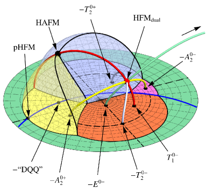
Figure 13: (a) The $J_{z\pm}>0$ phase diagram showing all four triple lines from Table 3 including the $\Delta_{I^{\prime}}<0$ portions where the triple degeneracy occurs in the irreps above the ground state (red region on the left of the plots in Fig. 4). Colors are the same as Footnotes 13 and 7. Each is a circle which winds around the line of “diabolical” $T_{1}$ locus (blue line), and all four intersect at the two HAFM points. Points where these lines intersect the $J_{z\pm}=0$ plane (left and right ends of plots in Fig. 4) are labeled $(I^{\prime})^{0\pm}$, where $\pm$ denotes the sign of $\Delta_{I^{\prime}}$: $+$ indicates this irrep is gapped and $-$ indicates it is the ground state. (b) The “ferro” versions of the three triple lines and two isolated triple points, with reversed signs of all couplings $H\to-H$. The Heisenberg-plus-$J_{z\pm}$ family (red circle, c.f. Fig. 7) with both $\Delta_{T_{1\pm}}\neq 0$ maps to itself, while the other three are mapped to new lines with triple degeneracies above the ground state. All four intersect at the two HFM points. The intersections with $J_{z\pm}=0$ are indicated with a minus sign compared to the same labels in (a). Note that HFM$\equiv-$HAFM, pHFM$\equiv-$pHAFM, and $T_{1}^{0-}=-T_{1}^{0+}$.

VI.6 Quantum Spin Liquids

In the future it will be interesting to study degenerate intersections of phases in more detail, and to determine whether any of them gives rise to a stable quantum spin liquid. Unfortunately in three dimensions there are few tools available to determine this. The only example where we have a meaningful level of analytical control is quantum spin ice, i.e. perturbing around the classical spin liquid point $J_{zz}>0$ with all other couplings zero. There, we can perform a direct mapping from the spin Hamiltonian to a U(1) lattice gauge theory Hamiltonian [30], where the $S_{i}^{z}$ operators map to electric field operators and the spin raising and lowering operators $S_{i}^{\pm}$ map to electric field raising and lowering operations $\exp(\pm iA),$ where $A$ is the lattice vector potential. This is only possible because the transverse fluctuations can be treated perturbatively on top of a classical Ising limit. This method—treating the classical ground state manifold as electric field eigenstates and spin-flipping terms as Wilson string operators—cannot be applied to study, say, the quantum HAFM, because the isotropic nature of the classical ground state means there is no preferred way to split spin operators into longitudinal and transverse components. Indeed the ground state of the quantum HAFM has been debated extensively, with the general view being that it exhibits some form of order, symmetry breaking, or dimensional reduction [113, 76, 115, 116, 117, 118].

It will, in the long term, be interesting to determine whether the various degenerate loci in the pyrochlore phase diagram host quantum spin liquids. In particular, it will be interesting to understand the quantum ground states along the four triply degenerate lines and how they merge together at the quantum HAFM point. Previous studies have classified various types of quantum spin liquid mean field ground state wavefunctions are compatible with the symmetries of the pyrochlore lattice [8, 119, 120, 121, 122]. Ref. [8] emphasized how these are closely related to the competition of various intertwined irrep orders. Beyond mean field analysis, numerical methods will be required. Unfortunately Quantum Monte Carlo algorithms are not generic enough to explore the entire phase diagram efficiently, and other powerful numerical methods like DMRG have extremely limited applicability in three dimensions. Recently, new pseudo-fermion functional renormalization schemes have been developed [123, 76, 124, 125, 57, 67], see Ref. [126] for a review. These methods can detect certain ordering instabilities and predict two-point correlation function, but involve uncontrolled approximations and so must be used in combinations with other numerical and analytical methods.

VII Triple Degeneracies in Excited States

While we have discussed so far the cataloging of cases which have large degeneracies in the ground state and the resulting zero-energy flat bands, it is interesting to note that these high degeneracies can still be present even when they are not at zero energy. Such excited state degeneracies do not come into play in the ground state determination but may leave interesting imprints on the excitations above the ground state, e.g. in the spin wave (magnon) spectrum. As such, we close by briefly discussing the loci in the phase diagram where triple degeneracies occur above zero energy. The effects of these enhanced degeneracies on the excitation spectrum within each phase will be an interesting topic for future study.

As mentioned previously, the triply-degenerate lines parameterized in Table 3 can be continued to negative $\Delta_{I^{\prime}}$ and form complete circles in the phase diagram, as is shown in Fig. 4. All four such lines wind non-trivially around the degenerate $T_{1}$ locus. They are shown in Fig. 13(a) in the $J_{z\pm}>0$ half of the phase diagram, along with the two triple points. All four cycles intersect at the two fourfold-degenerate HAFM points. Each line, labeled by a single irrep $I^{\prime}$ which is tuned while the others are kept degenerate, intersects the $J_{z\pm}=0$ plane at two points, one where $\Delta_{I^{\prime}}>0$ and one where $\Delta_{I^{\prime}}<0$, which we have marked and labeled as $(I^{\prime})^{0\pm}$ depending on the sign of $\Delta_{I^{\prime}}$. The $\Delta_{E}<0$ line is not shown in its entirety as the stereographic projection maps the $E^{0-}$ point far from the origin. The $(I^{\prime})^{0-}$ points are in a sense “centers” of their respective phases: they are the points where all three neighboring phases have equal and maximal gap, implying that these points are equidistant from all three phase boundaries. This can be seen in Fig. 4(c), where these points correspond to the left-most limit of each plot: the triply-degenerate irreps have $J_{I}=0$ at these points while $\Delta_{I^{\prime}}<0$ reaches its minimum value. The line where both $T_{1}$ irreps are tuned, corresponding to the Heisenberg-plus-$J_{z\pm}$ model discussed in Section V.1, is slightly different. It cannot be parameterized by $\Delta_{T_{1-}}/\Delta_{T_{1+}}$ because both go negative on part of the path, so we have parameterized it instead by the splitting of the two $T_{1}$ irreps. This lines passes through two special points in the $T_{1}$ phase, namely the Heisenberg ferromagnet and its dual. These may respectively be thought of as two different “centers” of the $T_{1}$ phase, because in Fig. 7 one can see that the $T_{1}$ phase appears to be the union of two roughly-spherical lobes centered on these two points.

These are not all of the triply degenerate cases, however, only the ones that are obtained from the four-fold degenerate HAFM by lifting the degeneracy of one irrep. The remaining ones are obtained by flipping the signs of all the couplings, i.e. changing the sign of the Hamiltonian $H\to-H$. This produces another set of triple lines which all intersect at the Heisenberg ferromagnet (HFM), shown in Fig. 13(b) along with two additional triple points, the pseudo-HFM and the ferromagnetic version of the DQQ (also appearing in Fig. 7). We have indicated the locations of the intersections of these lines with the $J_{z\pm}=0$ plane, labeled the same as in Fig. 13(a) but with a minus sign to indicate these are the “ferro” counterparts. The $I^{\prime}=T_{1}$ line (red), corresponding to the Heisenberg-plus-$J_{z\pm}$ model, is special because this family of Hamiltonians is mapped to itself under $H\to-H$. Since this line connects the HAFM and HFM points, it connects all of the triply-degenerate models together.

VIII Conclusion

In this paper we have considered in detail the structure of the classical phase diagram of rare-earth pyrochlore magnetic insulators with nearest-neighbor anisotropic interactions, described by the Hamiltonian Eqs. 4 and 5 with zero single-ion anisotropy.

In Section II we gave an intuitive derivation of the organization of spins into tensor order parameters, corresponding to the multipole moments of a single tetrahedron. We directly related the various tensor components to irreducible representations (irreps) of the tetrahedral symmetry group $T_{d}$, listed in Table 1, each of which corresponds to a ground state shown in Fig. 2. The presence of two copies of the $T_{1}$ irrep results in the canting cycle shown in Fig. 3. We described how different irreps are coupled together, were the 3-components vector irreps serve as “fluxes” with corresponding “charges” given by the three components of $A_{2}\oplus E$: raising the energy of a charge lowers the energy of its corresponding fluxes and vice-versa, and gapping a charge forces a zero-divergence condition on the corresponding flux.

In Section III we parameterized the model space—the space of equivalence classes of models differing by affine rescalings, topologically a 3-sphere—in terms of the relative irrep energies. This allowed us to perform an exhaustive search of all possible ground state degeneracies, which uncovered four triply-degenerate lines where three phases meet, listed in Table 3, all of which meet at the Heisenberg anti-ferromagnet point and its $J_{z\pm}$-dual, where all four phases become degenerate. Two isolated triple points also occur when $J_{z\pm}=0$.

In Section IV we visualized the structure of the phase diagram by using a stereographic projection from the unit 3-sphere in the space of the four local couplings to $\mathbbm{R}^{3}$. Since the phase diagram is reflection-symmetric about $J_{z\pm}=0$, we first mapped this stereographically in Fig. 5, which yields the phase diagram of non-Kramers pyrochlore magnets (for which $J_{z\pm}=0$). We then mapped the phase diagram for $J_{z\pm}\neq 0$ (allowed for Kramers doublets) in Footnote 13, which exposes all of the phase boundaries, the four triply-degenerate lines, and shows how they merge at the two four-fold degenerate HAFM points. We also noted the locus along which the two $T_{1}$ irreps are degenerate, which is a circle lying in the $J_{z\pm}=0$ plane. This locus pierces the $T_{1}\oplus T_{2}$ and $T_{1}\oplus E$ phase boundaries, giving rise to the two isolated triple points in the phase diagram.

In Section V we discussed the $T_{1}$-degenerate locus in more detail. Going around any path in parameter space that links it the canting angle winds by $\pi$. In Fig. 8 we showed how the phase diagram is foliated into 2-spheres on which the canting angle is constant, all of which intersection along the $T_{1}$-degenerate locus. This is analogous to “diabolical loci” which gives the phase diagram a topological structure not evident from energetic considerations alone. Adiabatically transporting the system around this locus within the $T_{1}$ phase will cause the spins to perform a half-rotation around the canting cycle illustrated in Fig. 3. There is a topological invariant associated to 1-parameter families of Hamiltonians which identifies how many times they wind around the locus. We briefly described a general framework for such loci in frustrated magnets made of corner-sharing clusters in terms of homotopy groups of PSO($n$), a topic we leave for future study.

In Section VI we considered how the enhanced degeneracies obtained by tuning degenerate irreps give rise to flat bands, and how these may lead to spin liquids. We provided a general discussion of the connection between flat bands and spin liquids, and discussed various ground state selection mechanisms that may co-opt the formation of a stable spin liquid. We provided an overview of known spin liquids on the pyrochlore lattice obtained from the anisotropic Hamiltonian, and in Tables 6, 6 and 6 provided a catalog of all flat band degeneracies in the phase diagram, and identified which combinations of irreps yield flat band degeneracies which are more than the sum of their parts versus trivially stacked. In Figs. 9 and 10 we provided reference structure factors computed in the self-consistent Gaussian approximation for various interesting flat band cases, and described the relation between fourfold pinch points and pinch lines observed ubiquitously in these models: Fig. 12 demonstrates the 3D structure of the pinched correlations at the intersection of pinch lines, which when cut produce fourfold pinch points.

Lastly, in Section VII we identified all loci in the phase diagram where three irreps are degenerate above the ground state, including both the continuation of the triple phase degeneracies into each phase along with their ferro-counterparts which all intersect at the Heisenberg ferromagnetic points. This is summarized in Fig. 13.

Beyond the issue of whether any of the flat band cases we have cataloged host stable quantum spin liquids, in the future it will be of interest to extend the analysis here to study the broader phase diagram of breathing pyrochlores, which can have different couplings on the two symmetry-inequivalent sets of tetrahedra and may host additional spin liquids [127, 23, 121]. Furthermore, there may be surprising physics to be gleaned within the ordered phases of the pyrochlore in the spectrum of (magnon) excitations, as evidenced by the extended $T_{1}$-degenerate locus and the various lines of high degeneracy in the band structure above zero energy. Lastly, it will be interesting to study in more detail the canting cycle in the pyrochlore and other frustrated magnets, to explore its potential connections to diabolical loci, symmetry pumps, and boundary symmetry breaking, and whether it has experimentally observable consequences.

Appendix A Coordinate Conventions

Although not crucial for the results presented in this paper, for completeness we provide a set of coordinates for the local bases and parameterizations discussed throughout the paper. Defining the cubic axes of the pyrochlore crystal structure to be along the three Cartesian axes $\hat{\bm{e}}_{x},\hat{\bm{e}}_{y},\hat{\bm{e}}_{z}$, the FCC primitive vectors can be given by

$$\bm{a}_{1}=a_{0}\frac{\hat{\bm{e}}_{x}+\hat{\bm{e}}_{y}}{2},\quad\bm{a}_{2}=a_{0}\frac{\hat{\bm{e}}_{y}+\hat{\bm{e}}_{z}}{2},\quad\bm{a}_{3}=a_{0}\frac{\hat{\bm{e}}_{z}+\hat{\bm{e}}_{x}}{2},$$ (90)

where $a_{0}$ is the cubic conventional cell lattice constant. The four FCC sublattice vectors, corresponding to the four corners of a tetrahedron, can then be given by

$$\bm{c}_{1}=\bm{0},\quad\bm{c}_{2}=\bm{a}_{1}/2,\quad\bm{c}_{3}=\bm{a}_{2}/2,\quad\bm{c}_{4}=\bm{a}_{3}/2.$$ (91)

The centers of the tetrahedra form a bipartite diamond lattice with sublattice positions

$$\bm{\delta}_{\pm}=\pm\frac{1}{4}\sum_{\mu=1}^{4}\bm{c}_{\mu},$$ (92)

where we use $\mu$ to index the FCC sublattices of the pyrochlore lattice. The four sublattice easy-axis vectors can be then be specified by normalizing the displacement vector from the center of a tetrahedron to each corner,

$$\hat{\bm{z}}_{\mu}=\frac{\bm{c}_{\mu}-\bm{\delta}_{+}}{|\bm{c}_{\mu}-\bm{\delta}_{+}|}.$$ (93)

Using the notation

$$[abc]\equiv a\hat{\bm{e}}_{x}+b\hat{\bm{e}}_{y}+c\hat{\bm{e}}_{z}$$ (94)

along with $\bar{a}\equiv-a$, we can provide bases for the local frames at each corner of the tetrahedron (up to normalization),

$$\hat{\bm{x}}_{1} \propto[11\bar{2}]\quad\hat{\bm{x}}_{2}\propto[\bar{1}\bar{1}\bar{2}]\quad\hat{\bm{x}}_{3}\propto[\bar{1}12]\quad\hat{\bm{x}}_{4}\propto[1\bar{1}2]$$

$$\hat{\bm{y}}_{1} \propto[1\bar{1}0]\quad\hat{\bm{y}}_{2}\propto[\bar{1}10]\quad\hat{\bm{y}}_{3}\propto[\bar{1}\bar{1}0]\quad\hat{\bm{y}}_{4}\propto[110]$$

$$\hat{\bm{z}}_{1} \propto[\bar{1}\bar{1}\bar{1}]\quad\hat{\bm{z}}_{2}\propto[11\bar{1}]\quad\hat{\bm{z}}_{3}\propto[1\bar{1}1]\quad\hat{\bm{z}}_{4}\propto[\bar{1}11].$$ (95)

These are shown in Fig. 14. The $\hat{\bm{x}}_{\mu}$ vectors have been chosen to lie in mirror planes, while the $\hat{\bm{y}}_{\mu}$ vectors lie along a $C_{2}$ rotation axis. With these convention, referring to Fig. 2 and Fig. 3, $\psi_{2}$ has all spins along $\hat{\bm{x}}_{\mu}$; $\psi_{3}$ has all spins along $\hat{\bm{y}}_{\mu}$, $T_{2}$ has two spins along $\hat{\bm{y}}_{\mu}$ and two along $-\hat{\bm{y}}_{\mu}$; $T_{1,\text{planar}}$ has two spins along $\hat{\bm{x}}_{\mu}$ and two along $-\hat{\bm{x}}_{\mu}$; $A_{2}$ has all spins along $\hat{\bm{z}}_{\mu}$; and $T_{1,\text{ice}}$ has two spins along $\hat{\bm{z}}_{\mu}$ and two along $-\hat{\bm{z}}_{\mu}$.

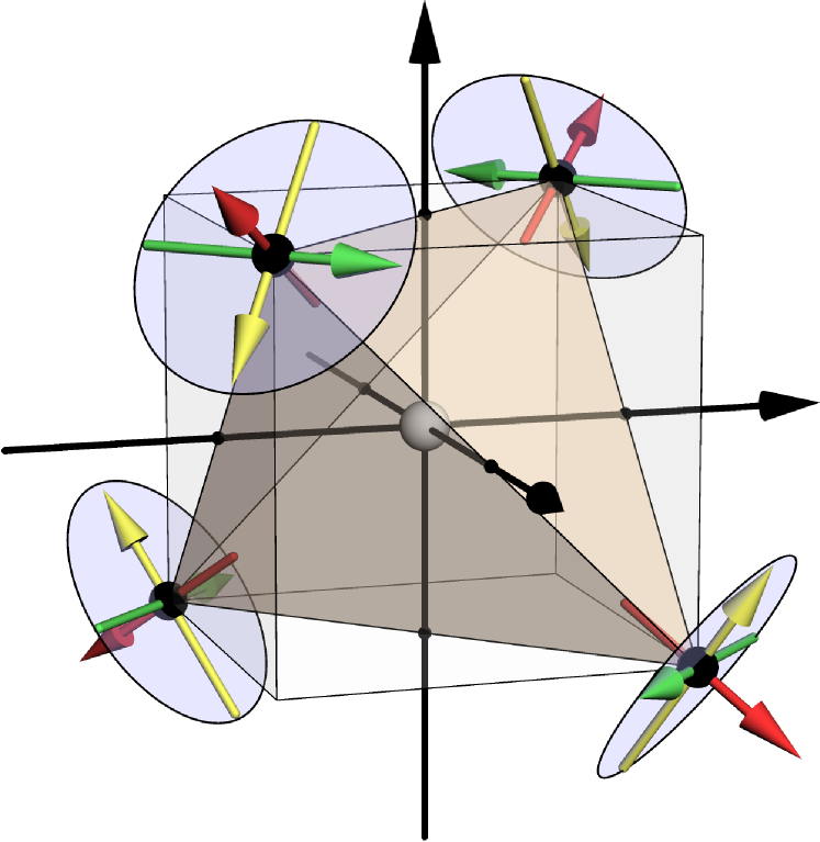
Figure 14: (a) A single tetrahedron inscribed in a cube showing the local orthonormal basis vectors defined in Eqs. 93 and 95. Red vectors are $\hat{\bm{z}}_{\mu}$ along the local three-fold easy axis. Yellow vectors are the $\hat{\bm{x}}_{\mu}$ which lie in mirror planes. Green vectors are the $\hat{\bm{y}}_{\mu}$ which lie along local $C_{2}$ axes which exchange neighboring tetrahedra. Note that the $\psi_{2}$ ($\psi_{3}$) configurations in Fig. 2 correspond to all spin lying along $\hat{\bm{x}}_{\mu}$ ($\hat{\bm{y}}_{\mu}$). Black arrows through the tetrahedron center denote the cubic [001] directions.

Appendix B Fourier Transforms

Due to translation invariance the interaction matrix in Eq. 2 is diagonal in the Fourier basis. We take the system to consist of $L^{3}$ unit cells with periodic boundaries, in which case

$$\mathcal{J}_{\mu\nu}^{\alpha\beta}(\bm{q},\bm{q}^{\prime}) \equiv\frac{1}{L^{3}}\sum_{i\in\mu}\sum_{j\in\nu}J_{ij}^{\alpha\beta}e^{i\bm{q}\cdot\bm{r}_{j}}e^{-i\bm{q}^{\prime}\cdot\bm{r}_{i}}$$

$$=\delta_{\bm{q},\bm{q}^{\prime}}\sum_{j\in\nu}J_{ij}^{\alpha\beta}e^{i\bm{q}\cdot(\bm{r}_{j}-\bm{r}_{j})}\quad(i\in\mu)$$

$$\equiv\delta_{\bm{q},\bm{q}^{\prime}}J_{\mu\nu}^{\alpha\beta}(\bm{q}),$$ (96)

where the sums are restricted to sites in a single sublattice. For nearest-neighbor interactions it is useful to define a modified adjacency matrix of the pyrochlore lattice,

$$\mathcal{A}_{ij}=\begin{cases}1&\quad\text{$i,j$ are nearest-neighbors,}\\ 1/2&\quad i=j,\\ 0&\quad\text{otherwise,}\end{cases}$$ (97)

whose Fourier transform is

$$\mathcal{A}_{\mu\nu}(\bm{q})=(2-\delta_{\mu\nu})\cos[\bm{q}\cdot(\bm{c}_{\mu}-\bm{c}_{\nu})].$$ (98)

The Fourier transformed nearest-neighbor interaction matrix is then

$$\mathcal{J}_{\mu\nu}^{\alpha\beta}(\bm{q})=J_{\mu\nu}^{\alpha\beta}\,\mathcal{A}_{\mu\nu}(\bm{q}),$$ (99)

where the $12\times 12$ matrix $J_{\mu\nu}^{\alpha\beta}$ is given in Eq. 102. The on-site term in Eq. 97 is added to allow for the on-site single-ion anisotropy interaction, which is double counted in the unrestricted double sum in Eq. 2. For reciprocal space we use Miller indices relative to the cubic conventional unit cell, denoted with round brackets

$$\bm{q}=\frac{2\pi}{a_{0}}(h\hat{\bm{e}}_{x}+k\hat{\bm{e}}_{y}+l\hat{\bm{e}}_{z})\equiv(hkl).$$ (100)

Appendix C Mapping Between Parameterizations

The number of free parameters in the interaction matrix $\mathcal{J}$ in Eq. 2 is restricted by symmetry. A given space group $G$ acts on the spin configuration $S_{i}^{\alpha}$ by permutation of the site index $i$ and pseudovector rotation of the spin components index $\alpha$. For nearest-neighbor interactions in the (non-breathing) pyrochlore lattice, the interaction matrix is the same on every tetrahedron, so the symmetry constraints can be obtained from just looking at the symmetry group of the tetrahedron, $T_{d}$, with action defined by the representation $\rho$ in Eq. 13. The allowed spin-spin couplings can be deduced from the fact that the Hamiltonian on a tetrahedron reduces to a sum over the irrep order parameters squared, or by looking for the solutions of

$$\mathcal{J}=\rho(g)\mathcal{J}\rho(g)^{-1}\quad\forall g\in G.$$ (101)

C.1 Global Frame $J_{1}$-$J_{4}$

With the conventions in Appendix A, the symmetry-allowed matrix elements in Eq. 2 for a single tetrahedron, denoted $\mathcal{J}_{\mu\nu}^{\alpha\beta}$ where $\mu,\nu$ index sublattices (tetrahedron corners), take the form

$$\begin{pmatrix}[c]\begin{pmatrix}[c]d&d&d\\ d&d&d\\ d&d&d\\ \end{pmatrix}&{\begin{pmatrix}[c]J_{1}&J_{3}&\bar{J}_{4}\\ J_{3}&J_{1}&\bar{J}_{4}\\ J_{4}&J_{4}&J_{2}\\ \end{pmatrix}}&\begin{pmatrix}[c]J_{1}&\bar{J}_{4}&J_{3}\\ J_{4}&J_{2}&J_{4}\\ J_{3}&\bar{J}_{4}&J_{1}\\ \end{pmatrix}&\begin{pmatrix}[c]J_{2}&J_{4}&J_{4}\\ \bar{J}_{4}&J_{1}&J_{3}\\ \bar{J}_{4}&J_{3}&J_{1}\\ \end{pmatrix}\\[4.30554pt] \begin{pmatrix}[c]J_{1}&J_{3}&J_{4}\\ J_{3}&J_{1}&J_{4}\\ \bar{J}_{4}&\bar{J}_{4}&J_{2}\\ \end{pmatrix}&\begin{pmatrix}[c]d&d&\bar{d}\\ d&d&\bar{d}\\ \bar{d}&\bar{d}&d\\ \end{pmatrix}&\begin{pmatrix}[c]J_{2}&J_{4}&\bar{J}_{4}\\ \bar{J}_{4}&J_{1}&\bar{J}_{3}\\ J_{4}&\bar{J}_{3}&J_{1}\\ \end{pmatrix}&\begin{pmatrix}[c]J_{1}&\bar{J}_{4}&\bar{J}_{3}\\ J_{4}&J_{2}&\bar{J}_{4}\\ \bar{J}_{3}&J_{4}&J_{1}\\ \end{pmatrix}\\[4.30554pt] \begin{pmatrix}[c]J_{1}&J_{4}&J_{3}\\ \bar{J}_{4}&J_{2}&\bar{J}_{4}\\ J_{3}&J_{4}&J_{1}\\ \end{pmatrix}&\begin{pmatrix}[c]J_{2}&\bar{J}_{4}&J_{4}\\ J_{4}&J_{1}&\bar{J}_{3}\\ \bar{J}_{4}&\bar{J}_{3}&J_{1}\\ \end{pmatrix}&\begin{pmatrix}[c]d&\bar{d}&d\\ \bar{d}&d&\bar{d}\\ d&\bar{d}&d\\ \end{pmatrix}&\begin{pmatrix}[c]J_{1}&\bar{J}_{3}&\bar{J}_{4}\\ \bar{J}_{3}&J_{1}&J_{4}\\ J_{4}&\bar{J}_{4}&J_{2}\\ \end{pmatrix}\\ \begin{pmatrix}[c]J_{2}&\bar{J}_{4}&\bar{J}_{4}\\ J_{4}&J_{1}&J_{3}\\ J_{4}&J_{3}&J_{1}\\ \end{pmatrix}&\begin{pmatrix}[c]J_{1}&J_{4}&\bar{J}_{3}\\ \bar{J}_{4}&J_{2}&J_{4}\\ \bar{J}_{3}&\bar{J}_{4}&J_{1}\\ \end{pmatrix}&\begin{pmatrix}[c]J_{1}&\bar{J}_{3}&J_{4}\\ \bar{J}_{3}&J_{1}&\bar{J}_{4}\\ \bar{J}_{4}&J_{4}&J_{2}\\ \end{pmatrix}&\begin{pmatrix}[c]d&\bar{d}&\bar{d}\\ \bar{d}&d&d\\ \bar{d}&d&d\\ \end{pmatrix}\end{pmatrix},$$ (102)

where for compactness we have used a bar to indicate a negative, $\bar{J}_{4}=-J_{4}$ and $\bar{d}=-d$, and defined $d=3J_{\text{SIA}}$ (c.f. Eq. 4). Equation 3 showed only the matrix elements for $\mu=1$ and $\nu=2$.

C.2 Global Frame Coordinate-Free

In Eq. 4 we provided another version of the Hamiltonian with various named interactions: Heisenberg, pseudo-dipolar, Kitaev-like, and Dzyaloshinskii-Moriya (DM). Their definitions are provided by Fig. 1. They are directly related to the global-basis parameters $J_{1}$ through $J_{4}$. It suffices to compare the interaction matrix $J_{\mu\nu}^{\alpha\beta}$ in Eq. 102 for a single pair $\mu\neq\nu$. With the conventions for the vectors given in Fig. 1 and Appendix A, we have the identification for sublattices $\mu=1$ and $\nu=2$

$$\begin{pmatrix}[c]J_{1}&J_{3}&-J_{4}\\ J_{3}&J_{1}&-J_{4}\\ J_{4}&J_{4}&J_{2}\end{pmatrix}=\begin{pmatrix}[c]J_{\text{Heis}}+J_{\text{PD}}/2&J_{\text{PD}}/2&J_{\text{DM}}/\sqrt{2}\\ J_{\text{PD}}/2&J_{\text{Heis}}+J_{\text{PD}}/2&J_{\text{DM}}/\sqrt{2}\\ -J_{\text{DM}}/\sqrt{2}&-J_{\text{DM}}/\sqrt{2}&J_{\text{Heis}}+J_{\text{K}}\end{pmatrix}.$$ (103)

C.3 Local Frame

To obtain the local basis Eq. 5, let $R_{\mu}$ denote the SO(3) matrices rotating from the global Cartesian basis $\{\hat{\bm{e}}_{x},\hat{\bm{e}}_{y},\hat{\bm{e}}_{z}\}$ to the local basis on each sublattice defined by Eq. 93 and Eq. 95, and let $Q$ denote the non-unitary transformation

$$Q=\begin{pmatrix}1&i&0\\ 1&-i&0\\ 0&0&1\end{pmatrix}:(S^{x}_{\mu},S^{y}_{\mu},S^{z}_{\mu})\mapsto(S^{+}_{\mu},S^{-}_{\mu},S^{z}_{\mu}),$$ (104)

let $R$ denote the block-diagonal matrix $\operatorname{diag}(R_{1},R_{2},R_{3},R_{4})$ and let $Q$ denote the block-diagonal matrix $\operatorname{diag}(Q,Q,Q,Q)$ Then the local couplings in Eq. 5 are obtained by transforming Eq. 102 as

$$\mathcal{J}_{\text{local}}=(Q^{-1})^{\dagger}\mathcal{R}\,\mathcal{J}_{\text{global}}\,\mathcal{R}^{-1}Q^{-1},$$ (105)

where $\scriptstyle{\dagger}$ denotes the conjugate transpose. Note that the complex phase factors appearing in Eq. 5 depend on the convention for the local bases. With the choice of basis from Appendix A, they are

$$\begin{pmatrix}[c]\begin{pmatrix}[l]0&0&0\\ 0&0&0\\ 0&0&1\end{pmatrix}&\begin{pmatrix}[c]1&1&1\\ 1&1&1\\ 1&1&-1\end{pmatrix}&\begin{pmatrix}[l]1&\omega^{2}&\omega\\ \omega&1&\omega^{2}\\ \omega^{2}&\omega&-1\end{pmatrix}&\begin{pmatrix}[l]1&\omega&\omega^{2}\\ \omega^{2}&1&\omega\\ \omega&\omega^{2}&-1\end{pmatrix}\\ \begin{pmatrix}[c]1&1&1\\ 1&1&1\\ 1&1&-1\end{pmatrix}&\begin{pmatrix}[l]0&0&0\\ 0&0&0\\ 0&0&1\end{pmatrix}&\begin{pmatrix}[l]1&\omega&\omega^{2}\\ \omega^{2}&1&\omega\\ \omega&\omega^{2}&-1\end{pmatrix}&\begin{pmatrix}[l]1&\omega^{2}&\omega\\ \omega&1&\omega^{2}\\ \omega^{2}&\omega&-1\end{pmatrix}\\ \begin{pmatrix}[l]1&\omega^{2}&\omega\\ \omega&1&\omega^{2}\\ \omega^{2}&\omega&-1\end{pmatrix}&\begin{pmatrix}[l]1&\omega&\omega^{2}\\ \omega^{2}&1&\omega\\ \omega&\omega^{2}&-1\end{pmatrix}&\begin{pmatrix}[l]0&0&0\\ 0&0&0\\ 0&0&1\end{pmatrix}&\begin{pmatrix}[c]1&1&1\\ 1&1&1\\ 1&1&-1\end{pmatrix}\\ \begin{pmatrix}[l]1&\omega&\omega^{2}\\ \omega^{2}&1&\omega\\ \omega&\omega^{2}&-1\end{pmatrix}&\begin{pmatrix}[l]1&\omega^{2}&\omega\\ \omega&1&\omega^{2}\\ \omega^{2}&\omega&-1\end{pmatrix}&\begin{pmatrix}[c]1&1&1\\ 1&1&1\\ 1&1&-1\end{pmatrix}&\begin{pmatrix}[l]0&0&0\\ 0&0&0\\ 0&0&1\end{pmatrix}\end{pmatrix},$$ (106)

where $\omega=e^{2\pi i/3}$. The relation between the global and local coupling parameters are given in Eqs. 7 and 8.

Appendix D SCGA Structure Factors

In the self-consistent Gaussian approximation (SCGA), the spin length constraint is relaxed to a Gaussian distribution whose variance is enforced by a Lagrange multiplier $\lambda$. Given a quadratic spin Hamiltonian $H$ of the form Eq. 2, we define the SCGA Hamiltonian

$$H_{\text{SCGA}}=H+T\sum_{i}\lambda_{i}|\bm{S}_{i}|^{2},$$ (107)

where $T$ is temperature. The partition function is then simply a multivariate Gaussian integral,

$$Z_{\text{SCGA}}=\int\prod_{i,\alpha}\mathrm{d}S_{i}^{\alpha}\,\exp(-\sum_{ij}\sum_{\alpha\beta}S_{i}^{\alpha}(\underbrace{\lambda_{i}\delta_{ij}\delta_{\alpha\beta}}_{\Lambda_{ij}^{\alpha\beta}}+\beta\mathcal{J}_{ij}^{\alpha\beta})S_{j}^{\beta}),$$ (108)

where $\beta=1/T$ is the inverse temperature and $\delta$ is the Kronecker delta. Correlation functions are then simply given by

$$\langle S_{i}^{\alpha}S_{j}^{\beta}\rangle\equiv\mathcal{G}_{ij}^{\alpha\beta}=([\Lambda+\beta\mathcal{J}]^{-1})_{ij}^{\alpha\beta}.$$ (109)

The Lagrange multipliers are solved for self-consistently via the constraint

$$1=\langle|\bm{S}_{i}|^{2}\rangle=\sum_{\alpha}([\Lambda+\beta\mathcal{J}]^{-1})_{ii}^{\alpha\alpha}.$$ (110)

Since every site is symmetry-equivalent in the pyrochlore lattice, the Lagrange multipliers are all the same, $\lambda_{i}\equiv\lambda$, and the self-consistency condition can be solved by averaging over all sites,

$$1=\frac{1}{N_{\text{spins}}}\operatorname{Tr}[\lambda\mathbbm{1}+\beta\mathcal{J}]^{-1},$$ (111)

where $\mathbbm{1}$ is the identity. We assume that the minimum eigenvalue of $\mathcal{J}$ has been shifted to zero, let $\mathscr{F}$ denote the kernel of $\mathcal{J}$, and let $N_{0}=\dim\mathscr{F}$ denote the number of zero eigenvalues of $\mathcal{J}$. In the limit of high temperature $\beta\to 0$ the solution is $\lambda=3$ (the number of spin components). In the low-temperature limit $\beta\to\infty$ all positive eigenvalues of $\mathcal{J}$ are suppressed in the inverse, and the solution is $\lambda=N_{0}/N_{\text{spins}}$. If $N_{0}$ is subextensive then $N_{0}/N_{\text{spins}}\to 0$ in the thermodynamic limit $N_{\text{spins}}\to\infty$, meaning that $\lambda$ vanishes at some critical temperature $T_{c}$, indicating a breakdown of the SCGA and a phase transition. If the number of zero eigenvalues is extensive, i.e. $\mathcal{J}$ has zero-energy flat bands, with $N_{0}=3N_{\text{spins}}f$ for $0<f=n_{\text{flat}}/n_{\text{tot}}<1$, then the solution is $\lambda=3f$. The zero-temperature correlation functions are then given by the projector $P_{\mathscr{F}}$ to the kernel of $\mathcal{J}$,

$$\lim_{T\to 0}\mathcal{G}=\frac{1}{3f}P_{\mathscr{F}}.$$ (112)

We use this formula to calculate the structure factor plots in Figs. 9 and 10.