Entanglement, loss, and quantumness: When balanced beam splitters are best

Abstract

The crux of quantum optics is using beam splitters to generate entanglement, including in pioneering experiments conducted by Hanbury-Brown and Twiss and Hong, Ou, and Mandel. This lies at the heart of what makes boson sampling hard to emulate by classical computers and is a vital component of quantum computation with light. Yet, despite overwhelming positive evidence, the conjecture that beam splitters with equal reflection and transmission probabilities generate the most entanglement for any state interfered with the vacuum has remained unproven for almost two decades [Asbóth et al., Phys. Rev. Lett. 94, 173602 (2005)]. We prove this conjecture for ubiquitous entanglement monotones by uncovering monotonicity, convexity, and entropic properties of states undergoing photon loss. Because beam splitters are so fundamental, our results yield numerous corollaries for quantum optics, from inequalities for quasiprobability distributions to proofs of a recent conjecture for the evolution of a measure of quantumness through loss. One can now definitively state: the more balanced a beam splitter, the more entanglement it can generate with the vacuum.

Beam splitters are foundational to entanglement generation [1], physical and mathematical models for optical loss and detector inefficiencies [2, 3, 4], mathematical descriptions of mode transformations in classical and quantum optics [5, 6, 7], interferometry [8, 9], and measuring wave-particle duality of light [10]. In terms of entanglement, a quantum state interfered with the vacuum at a beam splitter will generate two-mode entanglement if and only if the impinging state is nonclassical [11, 12, 13]. This nonclassicality and entanglement generation capability is prerequisite for the classical intractability of boson sampling [14, 15, 16, 17] and photonic quantum computation [18, 19, 20, 21, 22, 23, 24].

Entanglement is a hallmark of quantum theory [25, 26, 27] and crucial to many of its practical advantages [28, 29, 30, 31, 32], making entanglement’s manipulation, generation, and characterization essential. The entangling properties of beam splitters have been studied from many perspectives [33, 34, 35, 36, 37, 38, 39, 40, 41, 42, 43, 44, 45, 46, 47, 48], for example implying an important result for noisy quantum channels [49] and being crucial for distributing and measuring entanglement in quantum networks and communication [50, 51, 52]. Naturally, it led to a quantification of optical nonclassicality called entanglement potential: the amount of entanglement a single-mode state can generate at a beam splitter when interfered with the vacuum [37]; this has been measured experimentally [53, 54, 55, 56, 57]. When entanglement potential was defined, using any of a number of entanglement quantifiers, it was anecdotally observed that the most entanglement for any input state was always generated at perfectly balanced beam splitters with equal transmission and reflection probabilities of 50% [36, 37, 38, 58, 59, 60, 61, 62].

A general proof is still lacking [63]: The optimality for Gaussian states is straightforward [36, 38, 64]; proofs for Fock states can be gleaned from the statistics literature [65, 66, 67]; and powerful techniques such as majorization only help with comparing certain ranges of transmission probabilities [68, 69]. Entropy power inequalities for states input to beam splitters [70, 71] cannot help. We prove this property for all states.

We quantify entanglement in terms of ubiquitously used entanglement monotones and show that balanced beam splitters generate the most entanglement. Because different monotones only bound each other [72, 73, 74], a proof of optimality or convexity of one does not guarantee a proof for another. We start in Theorem 4 with entanglement entropy, which is singled out for its asymptotic continuity and which is important for many fields including condensed matter physics [75], quantum gravity [76], and uncertainty relations [77]. As well, many mixed-state entanglement monotones reduce to entanglement entropy for pure states, including distillable entanglement and relative entropy of entanglement (as in the original conjecture) [78, 79]. We then focus in Theorem 7 on entanglement measures based on purity such as Rényi 2-entropy, linear or collision entropy, and Tsallis 2-entropy, which provide more powerful entanglement witnesses than all Bell–Clauser-Horne-Shimony-Holt tests [80]. Entanglement and linear entropy exhibit important convexity properties in terms of quantum states [81, 82, 83, 84] and now we demonstrate their concavity in terms of beam splitter transmission probability $T$ (and photon loss $1-T$). Then, for another concurrence monotone found from a pure state’s Schmidt coefficients’ geometric mean, we show in Theorem 9 monotonic behaviour on either side of $T\!=\!1/2$ and related concavity properties. For completeness, we extend in Theorem 11 the proof of the conjecture to mixed states showing that $T\!=\!1/2$ is the unique local and global optimum for entanglement generation, but demonstrate in Theorem 12 that it is false for higher-order Rényi entropies.

Our successful proof leads to important corollaries that we detail in our companion paper [85]. For example, the intimate connection between beam splitters and loss allows us to bound how much loss a quantum state can withstand before it can no longer be certified as nonclassical, especially for a quantity known as the quadrature coherence scale (QCS) for which our recent conjecture [86] motivated the present study. Our results also explain how states lose distinguishability when they are each subject to loss and give robust equalities and inequalities for quasiprobability distributions beyond known ones that only hold for particular classes of states. The theorems presented here are simple and, yet, the corollaries are numerous and far-reaching.

Definitions (beam splitters, loss, entanglement monotones)–A beam splitter mixes two modes via complex transmission and reflection coefficients. Without loss of generality, we consider a one-parameter family given by the real transmission probability $T$. Mathematically, a bosonic mode annihilated by $a$ impinging on a beam splitter with another bosonic mode ($b$) transforms with unitary $B(T)=\text{e}^{\arccos\sqrt{T}(ab^{\dagger}-a^{\dagger}b)}$ as [87]

$$a\to B(T)aB(T)^{\dagger}=\sqrt{T}a+\sqrt{1-T}b.$$ (1)

When the mode annihilated by $b$ begins in the vacuum and the other mode is any superposition of Fock states $|\psi\rangle\!=\!\sum_{n}\psi_{n}|n\rangle$, the resultant state is $B(T)|\psi,0\rangle=|\Psi_{T}\rangle=\sum_{n}\psi_{n}\sum_{m}\sqrt{\binom{n}{m}T^{m}(1-T)^{n-m}}|m,n-m\rangle$. For nonclassical $|\psi\rangle$, $|\Psi_{T}\rangle$ is always entangled [11, 12, 13]. Ignoring the mode annihilated by $b$ generates the standard model for optical loss, with transmission probability $T$. When the reduced state $\rho_{T}=\mathrm{Tr}_{b}[|\Psi_{T}\rangle\langle\Psi_{T}|]$ is not pure, $|\Psi_{T}\rangle$ is entangled. We may write $\rho_{T}=\mathcal{E}_{T}[\rho_{1}]$ for $\rho_{1}=|\psi\rangle\langle\psi|$, where the loss channel $\mathcal{E}_{\tau}$ can be extended mixed-state inputs $\rho_{1}$ by linearity; loss acts multiplicatively such that $\mathcal{E}_{T_{1}}\circ\mathcal{E}_{T_{2}}=\mathcal{E}_{T_{1}T_{2}}$.

The family of Rényi entropies $H_{\alpha}(\rho)=\tfrac{1}{1-\alpha}\log\mathrm{Tr}\rho^{\alpha}$ quantifies the stochasticity of $\rho$ and is defined as the limit thereto when $\alpha\in\{0,1,\infty\}$. They all vanish when $\rho$ is pure and are strictly positive otherwise. Among this family, we focus on the entanglement entropy of $\Psi_{T}$ that is the von Neumann entropy of $\rho_{T}$: $\mathcal{S}_{\psi}(T)=H_{1}(\rho_{T})=-\mathrm{Tr}[\rho_{T}\log\rho_{T}]$ [88]; the mixedness (or linear entropy) $\mathcal{M}_{\psi}(T)=1-\mathcal{P}_{\psi}(T)$, for purity $\mathcal{P}_{\psi}(T)=\mathrm{Tr}[\rho_{T}^{2}]=\text{e}^{-H_{2}(\rho_{T})}$ [89]; and, for finite-dimensional $\rho_{T}$ with rank $d$, the $G$-concurrence $\mathcal{G}_{\psi}(T)=d\det[\rho_{T}]^{1/d}$ [90] that features in $H_{\alpha}=\log d+\alpha\log\mathcal{G}+\mathcal{O}(\alpha^{2})$; these are greater than zero for all nonclassical inputs $\psi$ because then $\rho_{T}$ is mixed, so each quantifies the entanglement potentially generated by a pure state $\psi$. Each of these is an entanglement monotone because it is a concave or Schur-concave function of the Schmidt coefficients [91, 92]; the latter are the singular values of the matrix with components $M_{mn}(T)=\langle m,n|\Psi_{T}\rangle$ and the eigenvalues of $\rho_{T}$. The monotones are all analytic functions of $T\in(0,1)$ . If the Schmidt coefficients of the same initial state for different values of $T$ always majorized each other then Schur concavity would guarantee concavity with $T$ for all of these entanglement monotones, but such majorization properties do not hold [68], thereby enriching the problem.

Lemma 1 (Schmidt symmetry).

The Schmidt matrix of a pure state subject to loss obeys $M(1\!-\!T)=M(T)^{\top}$.

Proof.

For the SWAP operator defined by $S|m,n\rangle=|n,m\rangle$, we have $S|\Psi_{T}\rangle=|\Psi_{1-T}\rangle$, which is like physically swapping the two output ports of the beam splitter. Therefore $\langle m,n|\Psi_{T}\rangle=\langle n,m|\Psi_{1-T}\rangle$. ∎

Transposing a matrix does not change its singular values, so a direct consequence of Lemma 1 is that $|\Psi_{T}\rangle$ and $|\Psi_{1\!-\!T}\rangle$ have the same Schmidt coefficients. Lemma 1 implies, for example, $\mathcal{S}_{\psi}(T)=\mathcal{S}_{\psi}(1\!-\!T)$. Therefore, if the derivative of an entanglement monotone is always nonnegative on one side of $T\!=\!1/2$ (e.g., $\partial\mathcal{S}_{\psi}/\partial T\!\geq\!0\ \forall\ T\!<\!1/2$), it is always nonpositive on the other side ($\partial\mathcal{S}_{\psi}/\partial T\!\leq\!0\ \forall\ T\!>\!1/2$). The following two Lemmas reveal the concavity of entropy.

Lemma 2 (Derivative of entropy of entanglement).

$\partial\mathcal{S}_{\psi}/\partial T=\langle a^{\dagger}a\rangle_{\psi}\left(H(\tau_{T}||\rho_{T})-H(\sigma_{T}||\rho_{T})\right)$ for relative entropy $H(X||Y)=\mathrm{Tr}[X(\log X-\log Y)]$ and normalized states $\sigma_{T}\propto a\rho_{T}a^{\dagger}$ and $\tau_{T}\propto\sqrt{\rho_{T}}a^{\dagger}a\sqrt{\rho_{T}}$.

Proof.

Derivatives of lossy states are known from master equations for damped harmonic oscillators (sometimes with other loss parametrizations like $\text{e}^{-\gamma t}=\cos^{2}\theta=\eta=T$) [93]:

$$\frac{\partial\mathcal{S}_{\psi}(T)}{\partial T} =-\mathrm{Tr}\left[\frac{\partial\rho_{T}}{\partial T}\log\rho_{T}\right]$$ (2)

$$=\frac{1}{2T}\mathrm{Tr}[(2a\rho_{T}a^{\dagger}-a^{\dagger}a\rho_{T}-\rho_{T}a^{\dagger}a)\log\rho_{T}]$$

$$=\langle a^{\dagger} a\rangle_{\psi}\mathrm{Tr}\left[\left(\frac{a\rho_{T}a^{\dagger}}{\mathrm{Tr}[a^{\dagger}a\rho_{T}]}-\frac{\sqrt{\rho_{T}}a^{\dagger}a\sqrt{\rho_{T}}}{\mathrm{Tr}[a^{\dagger}a\rho_{T}]}\right)\log\rho_{T}\right],$$

where the third line uses the commutation of functions of $\rho_{T}$ and that $\mathrm{Tr}[a^{\dagger}a\rho_{T}]=T\langle\psi|a^{\dagger}a|\psi\rangle$. Next, noticing that $\sigma_{T}=WW^{\dagger}$ and $\tau_{T}=W^{\dagger}W$ have the same eigenvalues such that $\mathrm{Tr}[\sigma_{T}\log\sigma_{T}]=\mathrm{Tr}[\tau_{T}\log\tau_{T}]$ and selecting $W=a\sqrt{\rho_{T}}/\sqrt{\mathrm{Tr}[a^{\dagger}a\rho_{T}]}$, we add and subtract $\langle a^{\dagger}a\rangle_{\psi}\mathrm{Tr}[\sigma_{T}\log\sigma_{T}]$ to complete the proof. ∎

Lemma 3 (Symmetry of relative entropy about loss).

$H(\tau_{T}||\rho_{T})=H(\sigma_{1-T}||\rho_{1-T})$.

Proof.

First write $X=\sum_{n}K_{n}|\psi\rangle\langle n|$ for Kraus operators $K_{n}(T)=\langle n|B(T)|0\rangle_{b}=\sqrt{T}^{a^{\dagger}a}(\sqrt{1-T}a)^{n}/\sqrt{n!}$ [94] such that $\rho_{T}=XX^{\dagger}$. Our notation suppresses $T$ dependence for brevity. Any operator $X$ satisfies $\sqrt{XX^{\dagger}}\log\left(XX^{\dagger}\right)\sqrt{XX^{\dagger}}=X\log\left(X^{\dagger}X\right)X^{\dagger}$. Thus

$$\mathrm{Tr}[\tau_{T}\log\rho_{T}]=\mathrm{Tr}\left[\frac{X^{{\dagger}}a^{{\dagger}}aX}{\mathrm{Tr}\left[a^{{\dagger}}aXX^{\dagger}\right]}\log\left(X^{{\dagger}}X\right)\right]$$ (3)

and $H_{1}[\tau_{T}]\!=\!H_{1}[\frac{X^{{\dagger}}a^{{\dagger}}aX}{\mathrm{Tr}\left[a^{{\dagger}}aXX^{\dagger}\right]}]$. Next, using $aK_{n}\!=\!\sqrt{T}K_{n}a$ (see [95]) and $\sum_{n}K_{n}^{\dagger}K_{n}=\openone$, we find

$$\frac{X^{\dagger}a^{\dagger}aX}{\mathrm{Tr}(X^{\dagger}a^{\dagger}aX)}=\frac{T\sum_{m,n}K_{m}^{\dagger}K_{n}|m\rangle\langle\psi|a^{\dagger}a|\psi\rangle\langle n|}{T\sum_{n}K_{n}^{\dagger}K_{n}\langle\psi|a^{\dagger}a|\psi\rangle}=Y^{\dagger}Y$$ (4)

for $Y=\sum_{n}K_{n}a|\psi\rangle\langle n|/\sqrt{\langle a^{\dagger}a\rangle_{\psi}}$. This means that $H(\tau_{T}||\rho_{T})=H(Y^{\dagger}Y||X^{\dagger}X)$. Next, note that $X$ and $Y$ are the Schmidt matrix representations of $B(T)|\psi,0\rangle$ and $B(T)a|\psi,0\rangle/\sqrt{\langle a^{\dagger}a\rangle_{\psi}}$. Lemma 1 reveals that

$$H(\tau_{T}||\rho_{T}) \!=\!H(Y(1\!-\!T)^{*}Y(1\!-\!T)^{\top}\!||X(1\!-\!T)^{*}X(1\!-\!T)^{\top}\!)$$ (5)

$$\!=\!H(Y(1\!-\!T)Y(1\!-\!T)^{\dagger}||X(1\!-\!T)X(1\!-\!T)^{\dagger}).$$

The last line follows because entropy is real; transposition and complex conjugation are always taken with respect to the Fock basis throughout this work. Finally, notice $X(1\!-\leavevmode\nobreak\ \!T)X(1\!-\!T)^{\dagger}\!=\!\rho_{1\!-\!T}$ and $Y(1\!-\!T)Y(1\!-\!T)^{\dagger}\!=\!\sigma_{1\!-\!T}$. ∎

Theorem 4 (Concavity of entropy).

The von Neumann entropy of a state subject to loss is an everywhere concave function; $\partial^{2}H_{1}(\rho_{T})/\partial T^{2}\leq 0\,\forall T\in(0,1)\,\forall\rho_{T}=\mathcal{E}[\rho_{1}]$.

Proof.

By Lemmas 2 and 3, $\partial\mathcal{S}_{\psi}(T)/\partial T=\langle a^{\dagger}a\rangle_{\psi}\left(H(\sigma_{1-T}||\rho_{1-T})-H(\sigma_{T}||\rho_{T})\right)$. We will show that $H(\sigma_{T}||\rho_{T})$ increases monotonically with $T$; by symmetry, $H(\sigma_{1-T}||\rho_{1-T})$ must decrease with $T$ such that $\partial\mathcal{S}_{\psi}/\partial T$ is nonincreasing with $T$.

This all follows because $\sigma_{T}$ is the result of the loss channel acting on $\sigma_{1}$ that enacts $\rho_{T}=\mathcal{E}_{T}[\rho_{1}]$ and such a channel $\mathcal{E}_{T}$ is completely positive and trace preserving. Since loss is multiplicative, for $T\leq T^{\prime}$, $H(\sigma_{T}||\rho_{T})=H(\mathcal{E}_{T/T^{\prime}}[\sigma_{T^{\prime}}]||\mathcal{E}_{T/T^{\prime}}[\rho_{T^{\prime}}]|)\leq H(\sigma_{T^{\prime}}||\rho_{T^{\prime}})$, where the inequality holds by the monotonicity of relative entropy [83]. The relevant assertion is proven by

$$\sigma_{T} =\frac{a\mathcal{E}_{T}[\rho_{1}]a^{{\dagger}}}{T\ \mathrm{Tr}\left(a^{{\dagger}}\rho_{1}a\right)}=\sum_{n}\frac{aK_{n}\rho_{1}K_{n}^{\dagger}a^{{\dagger}}}{T\ \mathrm{Tr}\left(a^{{\dagger}}\rho_{1}a\right)}$$ (6)

$$=\sum_{n}K_{n}\frac{a\rho_{1}a^{{\dagger}}}{\ \mathrm{Tr}\left(a^{{\dagger}}\rho_{1}a\right)}K_{n}^{\dagger}=\mathcal{E}_{T}[\sigma_{1}],$$

again using $aK_{n}=\sqrt{T}K_{n}a$ . Thus, $\partial^{2}\mathcal{S}_{\psi}(T)/\partial T^{2}\leq 0\,\forall T\in(0,1)\,\forall\psi$. Concavity for mixed states $\rho_{1}$ is proven in [95]. ∎

Corollary 5.

The entanglement entropy of a pure state interfered with the vacuum on a beam splitter is concave in beam splitter transmission probability and maximized at $T\!=\!1/2$.

Proof.

By Theorem 4, the entropy of the reduced density matrix $\rho_{T}$ is concave in $T$ and by Lemma 1 all pure states’ entanglement entropies are symmetric about $T=\leavevmode\nobreak\ 1/2$. ∎

Lemma 6 (Positive polynomial expansion of Hilbert-Schmidt norm).

The overlap between any two positive operators $\rho_{1}$ and $\sigma_{1}^{\dagger}$ subject to loss, as measured by the Hilbert-Schmidt inner product $O_{T}=\mathrm{Tr}[\rho_{T}\sigma_{T}]$, is a polynomial in $\lambda\equiv(1-2T)$ whose expansion coefficients are all nonnegative.

Proof.

Rewrite the inner product into a two-mode version using the SWAP operator $S=(-1)^{n_{-}}$ for $n_{i}=a^{\dagger}_{i}a_{i}$ and $a_{\pm}=(a_{1}\pm a_{2})/\sqrt{2}$ as $O_{T}=\mathrm{Tr}[\rho_{T}\otimes\sigma_{T}S]$ (this method has been used to measure purity using two copies of a state [80, 97]). Treating loss as beam splitters to vacuum modes annihilated by $b_{1}$ and $b_{2}$, noting that $|0\rangle_{b_{1}}\!\otimes\!|0\rangle_{b_{2}}\!=\!|0\rangle_{b_{+}}\!\otimes|0\rangle_{b_{-}}$ and $B_{a_{1}b_{1}}(T)B_{a_{2}b_{2}}(T)\!=\!B_{a_{+}b_{+}}(T)B_{a_{-}b_{-}}(T)$, and using cyclic permutations inside the trace to set $\langle 0|B_{a_{+}b_{+}}^{\dagger}B_{a_{+}b_{+}}|0\rangle_{b_{+}}=\openone_{a_{+}}$:

$$\mathrm{Tr}[ B_{a_{1}b_{1}}B_{a_{2}b_{2}}{\rho_{1}}\otimes{\sigma_{1}}\otimes|0,0\rangle\langle 0,0|_{b_{1},b_{2}}B_{a_{1}b_{1}}^{\dagger}B_{a_{2}b_{2}}^{\dagger}\ (-1)^{\hat{n}_{-}}]$$ (7)

$$=\mathrm{Tr}[{\rho_{1}}\otimes{\sigma_{1}}\langle 0|B_{a_{-}b_{-}}^{\dagger}\ (-1)^{\hat{n}_{-}}B_{a_{-}b_{-}}|0\rangle_{b_{-}}]$$

Then resolving the identity over states $|n\rangle_{b_{-}}$ and noting the Kraus operators for loss to be $\langle n|B_{a_{-}b_{-}}|0\rangle_{b_{-}}=\sqrt{T}^{n_{-}}(\sqrt{1-T}a_{-})^{n}/\sqrt{n!}$ as in Lemma 3, we sum $\sum_{n\geq 0}(1-T)^{n}a^{\dagger n}(-T)^{a^{\dagger}a}a^{n}/n!=\sum_{m\geq 0}(1\!-\!2T)^{m}|m\rangle\langle m|$ (as may be verified by matrix elements in the Fock basis) and recognize $B_{a_{1}a_{2}}(\tfrac{1}{2})a_{2}B_{a_{1}a_{2}}(\tfrac{1}{2})^{\dagger}=a_{-}$ to find

$$O_{T}\!=\!\sum_{m\geq 0}\!\lambda^{m}\mathrm{Tr}[({\rho_{1}}\otimes{\sigma_{1}})B_{a_{1}a_{2}}(\tfrac{1}{2})(\openone\!\otimes\!|m\rangle\langle m|)B_{a_{1}a_{2}}(\tfrac{1}{2})^{\dagger}].$$ (8)

Each term $B_{a_{1}a_{2}}(\tfrac{1}{2})(\openone\!\otimes\!|m\rangle\langle m|)B_{a_{1}a_{2}}(\tfrac{1}{2})^{\dagger}$ is a projection operator and thus its trace against a positive operator is always positive. ∎

Theorem 7 (Concavity of mixedness/convexity of purity).

The purity of a pure state subject to loss $\mathcal{P}_{\psi}(T)$ is an everywhere convex function and likewise the mixedness $\mathcal{M}_{\psi}(T)$ is everywhere concave; $\partial^{2}\mathcal{P}_{\psi}(T)/\partial T^{2}\geq 0\,\forall T\in(0,1)\,\forall\psi$.

Proof.

By Lemma 6, $\mathcal{P}_{\psi}(T)=\sum_{m\geq 0}\lambda^{m}p_{m}$ for coefficients $p_{m}\geq 0$. By symmetry about $T\!=\!1/2$ ($\lambda=0$), $p_{m}=0$ for all odd $m$. The second derivative is therefore comprised solely of positive terms $\frac{\partial^{2}\mathcal{P}}{\partial T^{2}}=\sum_{l>0}4(2l)(2l-1)\lambda^{2l-2}p_{2l}>0$. ∎

Corollary 8.

The entanglement of a pure state interfered with the vacuum on a beam splitter as measured by purity of the reduced state is convex in beam splitter transmission probability and maximized at $T\!=\!1/2$.

Proof.

By Theorem 7, the entropy of the reduced density matrix $\rho_{T}$ is convex in $T$ and by Lemma 1 all pure states’ reduced systems’ purities are symmetric about $T\!=\!1/2$. ∎

Theorem 9 (Monotonicity of concurrence).

The $G$-concurrence of a finite-dimensional pure state subject to loss is an everywhere nondecreasing (nonincreasing) function for $T<(>)1/2$ and its logarithm is concave; $\partial\mathcal{G}/\partial T\geq(\leq)\leavevmode\nobreak\ 0\,\ \forall\,T\leq(\geq)1/2\,\forall|\{\psi_{n}\}|<\infty$ and $\partial^{2}\log\mathcal{G}/\partial T^{2}\leq\leavevmode\nobreak\ 0\forall T$.

Proof.

For finite-dimensional states, there is a maximal $N$ such that $\psi_{n}=0$ for all $n>N$. Then $M$ is an anti-triangular matrix with zeros below the main anti-diagonal. The singular values $\{s_{0},\cdots,s_{N}\}$ of $M$ are complicated, but their product can be computed using $\det[\rho_{T}]=\prod_{i=0}^{N}s_{i}=|\det M|$. As an anti-triangular matrix, the determinant of $M$ is given by the product of the entries on the main anti-diagonal, all multiplied by $(-1)^{N}(-1)^{N-1}\cdots$. Together,

$$\mathcal{G}_{\psi}(T)=(N+1)|\psi_{N}|\frac{\sqrt{N!}}{\prod_{n=0}^{N}n!^{\tfrac{1}{N+1}}}[T(1-T)]^{\tfrac{N}{4}}.$$ (9)

Similar to the concavity of the matrix function $\log\det A$, we see that $\log\mathcal{G}\propto\log(T(1-T))$, which is manifestly concave with global maximum at $T\!=\!1/2$; the proof is completed using monotonicity of a logarithm with its argument. ∎

The extension of Theorem 9 to infinite dimensions is suspect: although the eigenvalues of a series of matrices $M_{N}$ converge to those of an infinite-dimensional matrix $M$ for all states with bounded energy [95], their product is discontinuous due to the inclusion of different numbers of eigenvalues for different $N$.

Since $\rho_{T}$ is full rank for $T\neq 0,1$, $H_{0}(\rho_{T})$ is also trivially concave in $T$, we now see that the first-order expansion coefficient in $H_{\alpha}-H_{0}$ is concave, so $H_{\alpha}$ for infinitesimal $\alpha$ is another entanglement monotone that is concave in $T$.

Corollary 10.

The entanglement of a pure state interfered with the vacuum on a beam splitter as measured by $G$-concurrence of the reduced state is maximized at $T\!=\!1/2$.

Proof.

By Theorem 9, the $G$-concurrence of the reduced density matrix $\rho_{T}$ has a global maximum at $T\!=\!1/2$. ∎

Definition (mixed-state entanglement)–For any pure-state entanglement monotone $E(\Psi)$, a mixed-state entanglement monotone can be defined by a convex-roof extension over all pure state decompositions [78, 79]: $\tilde{E}(\omega)=\inf_{\omega=\sum_{i}p_{i}|\Psi^{i}\rangle\langle\Psi^{i}|}\sum_{i}p_{i}E(\Psi^{i})$. Even for mixed input states $\rho_{1}$, all non-classical states interfering with the vacuum on a beam splitter always generate entanglement $\omega_{T}=B(T)\rho_{1}\otimes|0\rangle\langle 0|B(T)^{\dagger}$, where classical mixed states are defined as coherent states and convex mixtures thereof [98, 99, 100, 101]. We write the entanglement potentials for mixed states as $\tilde{\mathcal{F}}_{\rho_{1}}(T)=\tilde{E}(\omega_{T})$. For the von Neumann entropy this is known as the entanglement of formation [102] and for the purity this is known as the generalized or I-concurrence [103].

Theorem 11 (Mixed-state entanglement generated by beam splitters).

The entanglement generated by a beam splitter for any mixed state interfered with the vacuum is maximized at $T\!=\!1/2$ (i.e., at a balanced beam splitter) as measured by convex-roof extensions of $\mathcal{S}_{\psi}$, $\mathcal{M}_{\psi}$, and $\mathcal{G}_{\psi}$ as well as concave for $\mathcal{S}_{\psi}$, $\mathcal{M}_{\psi}$.

Proof.

The possible input-state decompositions $\rho_{1}=\sum_{i}p_{i}|\psi^{i}\rangle\langle\psi^{i}|$ are in one-to-one correspondence with the decompositions of the beam-splitter-entangled state $\omega_{T}=\sum_{i}p_{i}|\Psi_{T}^{i}\rangle\langle\Psi_{T}^{i}|$ due to $|\Psi^{i}_{T}\rangle=B(T)|\psi_{i}\rangle\otimes|0\rangle$. Then the infimum over two-mode states collapses to an infimum over input-state decompositions by $E(\Psi_{T})=\mathcal{F}_{\Psi}(T)$

$$\tilde{\mathcal{F}}_{\rho_{1}}=\inf_{\rho_{1}=\sum_{i}p_{i}|\psi^{i}\rangle\langle\psi^{i}|}\sum_{i}p_{i}\mathcal{F}_{\psi^{i}}(T)$$ (10)

and a convex sum of monotonic or concave functions that are each symmetric about $T=1/2$ will inherit the monotonicity or convexity and symmetry properties of its constituent terms. ∎

Theorem 12.

Not all entanglement monotones are concave in beam splitter transmission parameter or maximized at $T\!=\!1/2$.

Proof.

The Rényi entropies are all Schur-concave polynomials in a pure state’s Schmidt coefficients and thus bona fide entanglement monotones. For $\alpha=1$ and $\alpha=2$, Theorems 4 and 7, respectively prove that certain Rényi entropies are indeed concave in $T$ or monotonic in $|1-2T|$ for pure states subject to loss, and this is also true for infinitesimal values of $\alpha$ due to Theorem 9. Yet, this is not the case for all $\alpha$.

Take the Fock state $|\psi\rangle=|6\rangle$ subject to loss. We plot in Fig. 1 its Rényi entropy versus $T$ for various values of $\alpha$, from which it is clear that higher-order entropies need not be concave nor monotonic on either side of $T\!=\!1/2$ nor maximized at balanced beam splitters; related monotones like $\mathrm{Tr}[\rho_{T}^{12}]$, which are concave in Schmidt coefficients, are also not optimized at $T\!=\!1/2$. This reinforces that a unique calculation is required for each entanglement monotone and displays peculiarities of Rényi entropies with $\alpha>2$. ∎

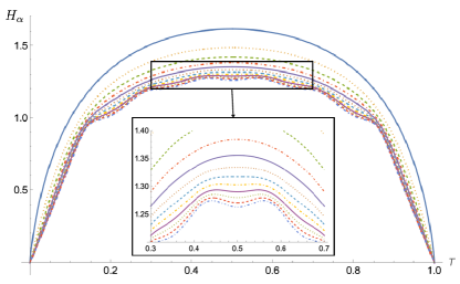
Figure 1: Rényi entropies from $\alpha=1$ (top, equal to von Neumann) to $\alpha=12$ (increasing downward) versus $T$ for a Fock state $|6\rangle$.

Theorems 4, 7, and 9 demonstrate for three entanglement monotones that the entanglement generated by a pure state interfered with the vacuum at a beam splitter will generate the most entanglement at a balanced beam splitter and Theorem 11 shows that this holds even for mixed-state inputs. This justifies the original definition of entanglement potential as the amount of entanglement generated by a state impinging on a balanced beam splitter [37], crowning it instead of alternatives such as the entanglement generated by infinitesimally transmissive beam splitters [104] or that averaged over beam splitter configurations [105]. Because beam splitters are intimately connected to loss, this also proves that quantities such as entropy and mixedness of a pure state are concave with loss, no matter their dimensionality or Gaussianity.

Loss, in turn, is intimately connected with damping, master equations, operator equations, and more. For example, we recently observed that the QCS seems to always stop certifying nonclassicality at 50% loss [86]. It turns out that this witness is equal to $1+T\partial\log(\mathcal{P})/\partial T$ [85] for any state and only certifies nonclassicality when it is $\geq 1$, which is now seen to coincide with transmission parameters greater than $50\%$ due to our present results that $\partial\mathcal{P}/\partial T\leq 0$ for $T\leq 1/2$. This is similar to but distinct from all quantum states losing Wigner negativity, another form of nonclassicality, when $T\leq 1/2$ [106], which touches upon the classical simulability of boson sampling arising from high photon loss that makes states lose their quantumness [107, 108, 109] and the rate-loss tradeoff for quantum key distribution [110]. The 50% condition appears in a number of other places, including degradability properties of a channel switching at $T=1/2$ [111], certain (but not all [112, 113]) quantum key distribution schemes becoming useless after 50% loss [114], and balanced beam splitters often being ideal for interferometry [115, 116] and for quantum scissors [117]. The further implications for quasiprobability distributions and equalities and inequalities for all quantum states, as well as for distance measures and quantum mutual information, are too many to contain in this Letter, so we direct the interested reader to our companion paper [85]. Entanglement, loss, entropies, operator norms, and quantumness trade off with each other throughout quantum optics, so we are excited by the many implications of proving this conjecture. We expect similar studies of negativity- and distance-based entanglement measures to be equally fruitful.

SUPPLEMENTAL MATERIAL

Appendix A More detail for the proof of Lemma 3

The proof uses

$$aK_{n}=\sqrt{T}K_{n}a$$

where $K_{n}=\sqrt{T}^{a^{\dagger}a}\frac{(\sqrt{1-T}a)^{n}}{\sqrt{n!}}$ is the Kraus operator of the loss channel. This equality is proven using Baker–Campbell–Hausdorff identity and $[a^{\dagger}a,a]=-a$:

$$\sqrt{T}^{-a^{\dagger}a}a\sqrt{T}^{a^{\dagger}a} =e^{-a^{\dagger}a\ln\sqrt{T}}ae^{a^{\dagger}a\ln\sqrt{T}}$$

$$=a+[-a^{\dagger}a\ln\sqrt{T},a]$$

$$\ +\frac{1}{2!}[-a^{\dagger}a\ln\sqrt{T},[-a^{\dagger}a\ln\sqrt{T},a]]+\ldots$$

$$=ae^{\ln\sqrt{T}}=a\sqrt{T}$$

$$\Rightarrow aK_{n} =\sqrt{T}K_{n}(T)a$$

Note that this can also be proven by looking at matrix elements in the number basis.

Appendix B Concavity of von Neumann entropy for mixed states $\rho_{1}$.

We extend the pure-state proof by writing

$$\tilde{X}(T)=\sum_{i}\sqrt{p_{i}}\sum_{n}K_{n}(T)|\psi^{i}\rangle\langle n|\otimes|0\rangle\langle\psi^{i\ast}|.$$ (11)

Here we have added an extra degree of freedom to take care of the mixedness of the initial, lossless state $\rho_{1}=\sum_{i}p_{i}|\psi^{i}\rangle\langle\psi^{i}|$, where the coefficients are valid probabilities $p_{i}>0$ and the eigenstates $\{|\psi^{i}\rangle\}$ are orthonormal without loss of generality, and we employ the orthonormal states $\{|\psi^{i\ast}\rangle\}$ whose coefficients are the complex conjugates of $\{|\psi^{i}\rangle\}$’s in the Fock basis. Considering the state that purifies $\rho_{1}$ to be $|\Psi\rangle=\sum_{i}\sqrt{p_{i}}|\psi^{i},\psi^{i}\rangle$, we can write the above as $\rho_{1}=\mathrm{Tr}_{b}[|\Psi\rangle\langle\Psi|]$ and

$$\tilde{X}(T)^{\top} =\sum_{i}\sqrt{p_{i}}\sum_{n}(K_{n}(T)|\psi^{i}\rangle\langle n|)^{\top}\otimes|\psi^{i}\rangle\langle 0|$$ (12)

$$=\sum_{i}\sqrt{p_{i}}\sum_{n}K_{n}(1-T)\otimes\openone|\psi^{i},\psi^{i}\rangle\langle n,0|$$

$$=\sum_{n}K_{n}(1-T)\otimes\openone|\Psi\rangle\langle n,0|$$

using the transpose of the Kraus operators proven for pure states. In this case, just like for pure states,

$$\tilde{X}(T)\tilde{X}(T)^{\dagger}=\mathcal{E}_{T}\otimes\openone[\rho_{1}\otimes|0\rangle\langle 0|]=\rho_{T}\otimes|0\rangle\langle 0|$$ (13)

from orthonormality of $\{|\psi^{i\ast}\rangle\}$ in the second degree of freedom and

$$\left(\tilde{X}(T)^{\dagger}\tilde{X}(T)\right)^{\ast} =\tilde{X}(T)^{\top}\tilde{X}(T)^{\top\dagger}$$ (14)

$$=\sum_{n}K_{n} (1-T)\otimes\openone|\Psi\rangle\langle\Psi|K_{n}(1-T)^{\dagger}\otimes\openone$$

$$=\mathcal{E}_{1-T}\otimes\openone[|\Psi\rangle\langle\Psi|].$$

Next, we adapt our pure-state proof to again use $\sqrt{XX^{\dagger}}\log\left(XX^{\dagger}\right)\sqrt{XX^{\dagger}}=X\log\left(X^{\dagger}X\right)X^{\dagger}$:

$$\mathrm{Tr}[a^{\dagger}a \rho_{T}\log\rho_{T}]=\mathrm{Tr}[\sqrt{\rho_{T}}a^{\dagger}a\sqrt{\rho_{T}}\log\rho_{T}]$$ (15)

$$=\mathrm{Tr}[\sqrt{\rho_{T}\otimes|0\rangle\langle 0|}(a^{\dagger}a\otimes\openone)\sqrt{\rho_{T}\otimes|0\rangle\langle 0|}$$

$$\qquad\times\log(\rho_{T}\otimes|0\rangle\langle 0|)]$$

$$=\mathrm{Tr}[\tilde{X}(T)^{\dagger}(a^{\dagger}a\otimes\openone)\tilde{X}(T)\log(\tilde{X}(T)^{\dagger}\tilde{X}(T))].$$

Similarly defining

$$\tilde{Y}(T) =\frac{(a\otimes\openone)\tilde{X}(T)}{\sqrt{\mathrm{Tr}[\tilde{X}^{\dagger}(a\otimes\openone)^{\dagger}(a\otimes\openone)\tilde{X}(T)]}}$$ (16)

$$=\frac{(a\otimes\openone)\tilde{X}(T)}{\sqrt{T\mathrm{Tr}[a^{\dagger}a\rho_{1}]}}$$

$$=\sum_{i}\sqrt{p_{i}}\sum_{n}K_{n}(T)\frac{a|\psi^{i}\rangle}{\sqrt{\langle\Psi|a^{\dagger}a\otimes\openone|\Psi\rangle}}\langle n|\otimes|0\rangle\langle\psi^{i\ast}|,$$

we find

$$\tilde{Y}(T)^{\top}=\sum_{n}\frac{K_{n}(1-T)a\otimes\openone|\Psi\rangle}{\sqrt{\langle\Psi|a^{\dagger}a\otimes\openone|\Psi\rangle}}\langle n,0|$$ (17)

using the transposition identity and thus

$$\mathrm{Tr}[a^{\dagger}a \rho_{T}\log\rho_{T}]=\mathrm{Tr}[a^{\dagger}a\rho_{T}\log\rho_{T}]^{\ast}$$ (18)

$$=\mathrm{Tr}[a^{\dagger}a\rho_{1}]\mathrm{Tr}[\tilde{Y}(T)^{\dagger}\tilde{Y}(T)\log(\tilde{X}(T)^{\dagger}\tilde{X}(T)]^{\ast}$$

$$=\mathrm{Tr}[a^{\dagger}a\rho_{1}]\mathrm{Tr}[\tilde{\sigma}_{1-T}\log\tilde{\rho}_{1-T}]$$

for analogously defined $\tilde{\rho}_{T}=\mathcal{E}_{T}\otimes\openone[|\Psi\rangle\langle\Psi|]$ and $\tilde{\sigma}_{T}=\mathcal{E}_{T}\otimes\openone[(a\otimes\openone)|\Psi\rangle\langle\Psi|(a^{\dagger}\otimes\openone)/\langle\Psi|a^{\dagger}a\otimes\openone|\Psi\rangle]$. We thus have

$$\frac{\partial H_{1}[\rho_{T}]}{\partial T}=\langle a^{\dagger}a\rangle_{\rho_{1}}\left(H(\tilde{\sigma}_{1-T}||\tilde{\rho}_{1-T})-H({\sigma}_{T}||{\rho}_{T})\right)$$ (19)

(no $\tilde{}$ on the second term) and monotonicity of relative entropy is again enough to establish that this is positive monotonically increasing with $T$ such that the entropy is always concave.

Appendix C Convergence of determinants in infinite dimensions

Lemma 13 (Entanglement convergence in infinite dimensions).

The Schmidt coefficients of an infinite-dimensional pure state with finite energy are equal to those found from a limit of finite-dimensional pure states.

Proof.

The squares of the Schmidt coefficients are the eigenvalues of the positive-definite matrix $MM^{\dagger}$ For a finite-dimensional state with maximal Fock number $N$, denote the matrix from which the Schmidt coefficients are found as $M_{N}$. We prove that the eigenvalues $\{\lambda_{i}\}$ of $M_{N}$ converge to those of $M$ as $M_{N}\to M$. First, note that the nonzero eigenvalues are the solutions of the equation $\det(\mathds{I}-A/\lambda)=0$ and that the Fredholm determinant $\det(\mathds{I}+A)$ is well-defined and continuous on trace-class operators $A$.

Next, defining the differences between the Fredholm determinants as $\delta=\left|\det(\mathds{1}-M/\lambda)-\det(\mathds{1}-M_{N}/\lambda)\right|$, the Fredhold determinant obeys the inequality

$$\delta\leq||M-M_{N}||_{1}\exp[\max(||M_{N}||_{1},||M||_{1})/|\lambda|+1]/|\lambda|.$$ (20)

The eigenvalues of $M$ and $M_{N}$ approach each other. This can be seen by verifying the trace $\mathrm{Tr}[M]=\sum_{n=0}^{\infty}|\psi_{n}|\sqrt{p_{n/2}(n;T)}<\infty$ and the norms $\sum_{m\geq 0,n>N}|\psi_{n}|\sqrt{p_{m}(n;T)}=||M-M_{N}||_{1}<||M||_{1}=\sum_{mn\geq 0}|\psi_{n}|\sqrt{p_{m}(n;T)}<\infty$, where we use the binomial probability $p_{m}(n;T)=\binom{n}{m}T^{m}(1-T)^{n-m}$. When $n$ is large, the binomial distribution tends to a normal distribution with mean $\mu=nT$ and variance $\sigma^{2}=nT(1-T)$. The trace of $M$ sums over the peaks of the square roots of this distribution, with values $p_{\mathrm{max}}(n;T)\approx(\sqrt{2\pi}\sigma)^{-1}=1/\sqrt{2\pi T(1-T)n}$. Assume the state has finite energy $\infty>\langle a^{\dagger}a\rangle=\sum_{n}|\psi_{n}|^{2}n$; then $|\psi_{n}|<\mathcal{O}(1/n)$. Then $\mathrm{Tr}(M)<\sum_{n}\mathcal{O}(n^{-3/2})<\infty$ (this is also true under the weaker condition that the state’s coefficients are normalizable, with $\sum_{n}|\psi_{n}|^{2}<\infty\Rightarrow|\psi_{n}|<\mathcal{O}(1/\sqrt{n})$).

Next, the one norms of the matrices are computed as the finite one norms of the $M_{N}$ plus the one norm of the extra components $||M||_{1}=||M_{N}||_{1}+||M-M_{N}||_{1}$. The latter, for sufficiently large $N$, can make use of the square root of a normal distribution, summed over all components. The square root of a normal distribution is also normal, with the same mean, but with a larger standard deviation $\sigma^{2}=2nT(1-T)$ and the whole distribution is multiplied by $\sqrt{\sqrt{2\pi nT(1-T)}}\sqrt{2}$. The sum over $p_{m}$ becomes an integral over the normal distribution, yielding the coefficient $\sim n^{1/4}$. We thus find $||M-M_{N}||_{1}=\sum_{n>N}|\psi_{n}|\mathcal{O}(n^{1/4})$. Choosing states with finite higher-order moments of energy, such as $\langle(a^{\dagger}a)^{3/2}\rangle<\infty\Rightarrow|\psi_{n}|<\mathcal{O}(n^{-5/2})$, ensures that $||M-M_{N}||_{1}<\sum_{n>N}\mathcal{O}(n^{1/4-5/4})<\infty$. Once these are all proven to be finite, the work is done: the norm decreases as $N$ gets bigger, one can make it as small as any parameter $\epsilon\to 0$, thus sending $\delta\to 0$.

Since the eigenvalues of $M$ approach those of $M_{N}$, the products of the eigenvalues of $M_{N}$ approach those of $M$. Then, so too does the product of Schmidt coefficients of the state and thus the finite-dimensional entanglement monotone given by the product of Schmidt coefficients seems to converge in the limit of infinite dimensions. However, the entanglement monotone for $N$ is given by $\prod_{i=0}^{N}s_{i}$ and for $N+1$ by $s_{N+1}\prod_{i=0}^{N}s_{i}$. While the latter is continuous with $s_{N+1}$, there is a discontinuity between the former and the latter, especially noticeable when $s_{N+1}\approx 0$. Should the entanglement monotone have been defined as $\prod_{i=0}^{\infty}s_{i}$ for all states, it would have always been continuous, but it would have been vanishingly small for all states. The entanglement monotone defined with determinants of reduced density matrices is thus only applicable for finite-dimensional states. ∎