Developing a Multi-grid Fortran Tool for PT-Table Generation in Terrestrial Planetary Atmospheres

MARFA: An Effective Line-by-line Tool for Calculating Absorption Coefficients and Cross-sections in Planetary Atmospheres

Abstract

We present MARFA (Molecular atmospheric Absorption with Rapid and Flexible Analysis) – a streamlined efficient tool for line-by-line calculation of atmospheric absorption signatures in the form of PT lookup tables, which may be used in radiative transfer codes. The tool is intended for computations in the IR and visible spectral regions. Core line-by-line scheme features nine-grid interpolation technique, which strikes good balance between speed and accuracy for calculations in the scenario of unknown continuum function and large lines cut-offs. The model features high flexibility, allowing fast recalculations with different line shapes, $\chi$-factors, line cut-offs conditions, and other parameters, making it valuable for planetary studies where atmospheric and spectroscopic data are sparse or uncertain. The MARFA tool is provided in two ways: through a web interface for onboarding and immediate usage, and as open-source code available in a public repository for advanced utilization, development and contributions.

Keywords planetary atmospheres  $\cdot$ molecular absorption  $\cdot$ line-by-line modeling  $\cdot$ absorption cross-sections  $\cdot$ radiative transfer

1.  Introduction

Since 1960s [1] a significant number of Line-By-Line (LbL) Radiative Transfer Models (RTMs) have been developed for modeling the radiative transfer in the atmospheres of Earth and other terrestrial planets. These models are crucial for situations when detailed (’ab-initio’) consideration of molecular absorption and emission spectra are required. Applications include remote sensing of planetary atmospheres, as well as reference radiative flux calculations necessary for weather and climate modeling. Precise atmospheric absorption calculations are essential in studies devoted to understanding and predicting atmospheric behavior and energy balance, which are vital for both scientific research and practical applications. One of the most notable models in this domain is the LBLRTM model [2, 3], which is central to the LbL methodology and has set standards for many subsequent generations of RTMs.

From a computational standpoint, there are three stages in a typical scheme for running LBLRTM. In the first stage, at the required altitude levels and spectral intervals, the profiles of significant spectral lines are calculated and summed into a function of the wavenumber, consisting of many sharp peaks. After that, continuum contributions are added to this function to obtain the required molecular spectra, which can be stored, for example, in PT-tables format and reused multiple times. Finally, the radiative transfer equations in the atmosphere are solved using the obtained spectra. The resulting quantities from the RTM solution may be either radiances and transmittances, primarily for matching experimental spectra, or fluxes and heating rates, mainly for weather and climate modeling. The combination of summing line profiles with the addition of a continuum function has proven to be an effective strategy, and this approach is employed in LBLRTM and other line-by-line models used for Earth’s atmosphere, producing reliable results for a variety of applications.

The continuum addition process involves a relatively smooth function and demands significantly less computational effort. In contrast, the summation of individual line profiles consumes majority of time required for spectrum generation. If the continuum function is limited or unavailable, as is the case for Venus [4, 5], then the far wings of the lines must be considered, which further increases computational demands. Despite the advances made by the LBLRTM and similar models, there is still a need for more flexible and efficient tools, especially for planetary atmospheres with limited or uncertain spectroscopic data, where the continuum function may be missing. To address these needs, we propose a line-by-line model primarily focused on the efficient calculation of molecular absorption spectra. This model is based on the well-established interpolation technique [6], which was highlighted in [7] for its efficiency in independent comparisons. Legacy version of the tool was successfully employed in remote sensing applications by [8]. Standard Voigt line shape estimation algorithm [9] is incorporated in the MARFA core, but more sophisticated functions can be easily introduced, as long as they conform to the specified Fortran abstract interface. Factually, MARFA capable of summing any line profiles, allowing users to integrate non-Voigt line-shapes (e.g. [10, 11, 12, 13]), as well as implementing sub-Lorentz profiles through the so called $\chi$-functions [14, 15].

The layout of this paper is as follows. In the next section, we explain the physical and computational basis under the core MARFA functionality. It includes brief overview of molecular absorption basis, line summation algorithm and discussion of the implemented spectroscopic features. Section 3 provides a specific application scenario for the tool, focusing on the atmosphere of Venus. We show in this section why and how Venus atmosphere is taken as a benchmark and give some sample spectra for various spectroscopic settings. Section 4 discusses the software design and data formats. Additionally, in this section we give some guidance on implementing custom features and outline the tool’s limitation. Finally, Section 5 concludes the paper with a summary and suggestions for future releases.

2.  Molecular spectra calculation framework

The purpose of the tool shapes the framework for spectra calculation, focusing on two main goals. Firstly, we aim to equip users with an efficient algorithm for line-by-line calculations of either absorption cross-sections or volume absorption coefficients, minimizing concerns about spectral interval size and line cut-off condition. Secondly, we seek to provide an easy accessible tool by eliminating data hardcoding, enabling smooth parameter input, and and supporting open-source contributions and development

For a quick start, predefined line shapes can be utilized. We have implemented the Lorentz, Gaussian and Voigt profiles which correspond to pressure-broadening, Doppler broadening and the combination of both effects respectively. Additionally we have introduced the Tonkov sub-Lorentz correction [16], which is recommended for Venus studies [5] and some additional sub-Lorentz corrections. Below, in subsection 2.1. we provide a brief overview of how these predefined line shapes have been incorporated. Subsection 2.3. includes a discussion on the line-by-line algorithm we employed, along with a short overview of existing methods.

2.1.  Predefined line shapes

Following the notation by [17], the volume absorption coefficient in the atmosphere can be found by summing the contributions from individual lines across species ($l$ index) and transitions ($j$ index), and then add the continuum function:

$$k_{\nu,\nu}=\sum_{j,l}n^{l}S_{n,j}^{l}f_{j}^{l}(\nu-\nu_{0,j}^{l})+k_{\nu}^{c}.$$ (1)

Our scheme is designed such that a separate calculation is required for each atmospheric species, and the continuum function estimation is not included. Resulting output value presented in the PT-table format might be either the volume absorption coefficient (typically in km^-1 for atmospheric modeling) or the absorption cross-section in cm²/molecule, so the expression 1 transforms into:

$$k(\nu;p,T)=n(p,T)\sum_{j}S_{j}(T)f_{j}(\nu-\nu_{0};\gamma(p,T))$$ (2)

$$\sigma(\nu;p,T)=\sum_{j}S_{j}(T)f_{j}(\nu-\nu_{0};\gamma(p,T))$$ (3)

In expressions 2 and 3 $S$ represents a temperature-dependent line intensity, while $f$ is a normalized line shape function, which depends on both temperature and pressure through the half-width at half-maximum (HWHM) $\gamma$. The parameter $\nu_{0}$ is a center of the line (wavenumber of a transition). The number density $n$ of the species can be determined, for example, from the atmospheric profile and the species’ abundance (usually in ppm). Since the number density in expression 2 is outside the sum, the program can easily switch between calculation the absorption coefficient and the cross-section.

Initial line-specific spectroscopic data, normally taken from spectroscopic databases like HITRAN [18, 19] or GEISA [20, 21], is required to determine entities under the summation sign in expressions 2 and 3. The Spectroscopy.f90 module in the source code contains routines for calculation of temperature- and pressure- dependent Lorentz ($\gamma_{\text{L}}$) and Doppler ($\alpha_{\text{D}}$) half-widths, temperature-dependent line intensities $S(T)$ and pressure-induced shifts  $\tilde{\nu_{0}}$  based on the initial spectral data. All these values are determined using the formulas from the HITRAN website documentation [22].

All the predefined line shapes can be accessed in the Shapes.f90 module. This module consists of list of functions, each corresponding to the specific line shape. Since in expressions 2 and 3 line shape function is always multiplied by the intensity, the similar structure is maintained within the function itself. Predefined Lorentz and Gaussian lines shapes are implemented exactly as per the well-known formulas:

$$f_{\text{L}}(\nu;\,p,T)=\frac{1}{\pi}\frac{\gamma_{\text{L}}}{\gamma_{\text{L}}^{2}+(\nu-\tilde{\nu_{0}})^{2}}\qquad$$ (4)

$$f_{\text{G}}(\nu;\,T)=\sqrt{\frac{\ln 2}{\pi\alpha_{D}^{2}}}\exp\left(-\frac{(\nu-\nu_{0})^{2}\ln 2}{\alpha_{D}^{2}}\right)\qquad$$ (5)

For practical applications the Voigt line shape is widely used, described by the convolutional integral of Lorentzian and Gaussian line shapes:

$$f_{\text{V}}(\nu-\nu_{0},\gamma_{L},\gamma_{G})=f_{\text{L}}\otimes f_{\text{G}}=\int_{-\infty}^{\infty}\mathrm{d}\nu^{\prime}\,f_{\text{L}}(\nu-\nu^{\prime},\gamma_{L})\times f_{\text{G}}(\nu^{\prime}-\nu,\gamma_{G})$$ (6)

It can be effectively represented using the Voigt function $K(x,y)$ [23]:

$$f_{\text{V}}\left(\nu-\nu_{0};\gamma_{\text{L}},\alpha_{\text{D}}\right)=\frac{\sqrt{\ln 2/\pi}}{\alpha_{\text{D}}}K(x,y),$$ (7)

$$K(x,y)=\frac{y}{\pi}\int_{-\infty}^{\infty}\frac{e^{-t^{2}}}{(x-t)^{2}+y^{2}}\,dt,$$ (8)

where $x=\frac{\sqrt{\ln 2}(\nu-\nu_{0})}{\alpha_{\text{D}}}$ and $y=\frac{\sqrt{\ln 2}\,\gamma_{\text{L}}}{\alpha_{\text{D}}}$.

Many studies have proposed routines for determining the Voigt function through distinct numerical expansions, mainly due to its close relation to the complex error function. To evaluate the Voigt function, we use the well-known algorithmic approach from [9], which was improved by [24]. This algorithm is known to be a fitting choice for the Fortran language, which is the primary choice in MARFA implementation. To speed up the estimation of the Voigt function far from the line center, we use Lorentz function as asymptotic approximation. This approach has been successfully adopted and tested in several studies, as noted in code intercomparison research [25, 26]. Overall accuracy turns to be around 1%. While our scheme does not claim to be the most accurate, though we have incorporated a trusted algorithm for the Voigt function computation into the MARFA core. Note, that our focus is not on achieving the utmost accuracy in line shapes but on providing users with the flexibility to introduce their own.

2.2.  $\chi$-factors

Experimental data suggest that the far wings of spectral lines deviate from Lorentz or Voigt behavior. To address this in Venus studies, we have implemented within MARFA several $\chi$-factors for CO₂ line shapes: [16], [27], [15] for CO₂ line shape functions. For example, Tonkov wing correction is implemented according to the following formula:

$$f(\nu-\nu_{0})=f_{\text{L}}(\nu-\nu_{0})\chi_{\text{Tonkov}}(\nu-\nu_{0}),$$ (9)

where $\chi$ is a given piece-wise correction function:

$$\chi_{\text{Tonkov}}=\begin{cases}1.084\exp(-0.027\;|\nu-\nu_{0}|)&\text{if }3\;\text{cm${}^{-1}$}\leq|\nu-\nu_{0}|\leq 150\;\text{cm${}^{-1}$},\\ 0.208\exp(-0.016\;|\nu-\nu_{0}|)&\text{if }|\nu-\nu_{0}|>150\;\text{cm${}^{-1}$},\\ 1&\text{otherwise}.\end{cases}$$ (10)

If the line cutoff condition exceeds 300 cm^-1, the additional piece should be added to the $\chi$-function according to [16], who considered distances from line centers up to 600 cm^-1. This implementation serves as an example for users, how to add their own sub-Lorentz profiles or wings corrections by means of a piece-wise $\chi$-function. Project documentation provides detailed instructions on how to manually add custom $\chi$-functions.

2.3.  Interpolation technique for the line-by-line modeling

Beside improved algorithmic approaches for Voigt function, interpolation techniques are essential for speeding-up line-by-line modeling. Notable works in this domain are: [28, 29, 30, 31, 32, 6, 33, 7, 34, 35]. The technique proposed by [36] is based on decomposition of line shape into several sub-functions, each estimated on the individual grid. It was used in FASCODE [37] and LBLRTM [3] (based on FASCODE) and later gave an impulse for developing this method further for other line shapes. However, this approach makes it challenging to maintain flexibility with input line shapes, as it requires recalculating sub-functions for each new line shape. To ensure universality, schemes independent on the specific line shape are necessary. The so called multi-grid approach addresses this, by making estimations on a sequence of grids with increasing step sizes regardless of the shape function. The concept behind these algorithm is straightforward: moving away from the center of a spectral line results in the profile becoming progressively smoother, as in the case of a Lorentzian wing, where the profile follows $\sim 1/(\nu-\nu_{0})^{2}$. The line profile is divided into sections corresponding to the number of grids. On the finest grid, the central, sharpest parts of the lines are summed. On the next, coarser grid, the smoother parts adjacent to the center are summed, and so on. Once all parts of the lines have been summed on their respective grids, the discrete functions obtained on these grids are interpolated onto the finest grid, resulting in the desired spectrum. Most studies use two or three grids with different interpolation methods, and optionally adjusting the grid step according to the atmospheric level to resolve the narrowest line within the given spectral interval [38].

We use the multi-grid interpolation technique described by [6], which was employed in the calculation of absorption coefficients by [7] and highlighted in several intercomparison studies [26, 25]. Given that large line cut-offs are a crucial scenario, three grids may not suffice to achieve the desired balance between speed and accuracy. To address this, our scheme employs nine grids with doubling steps. The step size for the finest grid is typically set to be 3-5 times smaller than the typical line half-width, and this value can be specified by user as an input. For most practical applications, nine grids with steps ranging from $0.001\;\text{cm}^{-1}$ to $2^{9}*0.001\approx 0.5\;\text{cm}^{-1}$ are sufficient to accurately describe the far wings of spectral lines. In future releases, it might be possible, however, to include customization options based on user input, allowing adjustments to the number of grids for more sophisticated scenarios.

Importantly, the interpolation requires significantly less computational time compared to calculating line profiles on each grid. Interpolations between coarse and fine grids are performed only once and are independent of the number of lines, making the computation time for spectra logarithmically dependent on the line’s half-width. We maintain the ratio of distances between points in adjacent grids during the interpolation process from coarse to fine grids, using a simple polynomial interpolation method. For a more detailed description of interpolation errors, we advise to refer to the original method paper [6].

3.  Venus as a benchmark scenario

3.1.  Why Venus ?

The idea of developing a separate tool for calculating molecular spectra originated during our ongoing work on constructing k-distribution parameterizations suitable for Venus GCMs [39], and particularly in the IR and visible spectral intervals (in progress). We faced considerable uncertainty in Venus’ spectroscopic and atmospheric parameters, necessitating rapid recalculation of spectra for testing and validating purposes when running a forward model. In Section 3.2., we provide a brief overview of the key challenges and uncertainties in the data, which are crucial for accurately calculating absorption coefficients.

In our view, Venus is a good starting point for validation and testing of new general purpose line-by-line models, which aim to adhere to data-driven and flexible approach. Over the past six decades, Venus has been extensively studied through ground-based observations and flyby missions, resulting in a wealth of data. However, when it comes to radiative transfer modeling, reliable atmospheric and spectroscopic data to lay to the core of forward models remain limited. As RTMs are highly sensitive to atmospheric and spectroscopic parameters [5], it is crucial that these models treat such data strictly as inputs, rather than hardcoding them. This limitation is why many Earth-based or data-specific models struggle to capture Venusian conditions accurately. Moreover, Venus’ unique rotation characteristics and its location within the habitable zone provide a clear analogy to a telluric exoplanet [40, 41]. This makes it a promising test case for validating exoplanetary radiative transfer models.

3.2.  Challenges and uncertainties in Venus atmosphere modeling

For each radiatively active atmospheric constituent, pre-calculated absorption coefficients are available across various temperature and pressure values. Significant differences in thermal structure with respect to latitude and local time (solar longitude) are observed in models of Venus’s middle atmosphere [42, 43]. Temperature profiles in the upper atmosphere differ drastically between the day- and night-side hemispheres [44, 45, 46]. The temperature structure of the lower atmosphere is not well-studied and is often assumed to be homogeneous across the planet (globally averaged) in models. Given this, interpolation and averaging procedures are necessary, leading to multiple approaches for compiling an a priori initial temperature profile for retrieval procedures [47, 48].

Radiative heating and cooling rates are generally calculated up to a height of 150 km [5], requiring that constituent mixing ratio profiles also extend to this altitude. Most models use data compiled from various sources, interpolating to constant values in the upper atmosphere [49, 15, 5]. However, there is significant variability and data limitations, which future experimental data may help address.

The selected database for line parameters greatly affects the absorption cross-section and the resulting radiance spectra. Unfortunately, there is no dedicated Venus database with line parameters for all relevant species that accounts for CO₂ broadening and high-temperature conditions. As a result, line parameters for Venus modeling are typically taken from various databases and dedicated experimental studies [4, 48, 5]. Commonly used databases include HITRAN [50, 51, 52, 19, 18], HITEMP [53, 54], CDSD [55], and specific CO₂ data from HITEMP-VENUS [15]. It is important to note that the hot lower atmosphere of Venus presents an additional computational challenge because the use of HITEMP or HITEMP-VENUS databases is generally required over HITRAN. This results in an increase of spectral lines by two orders of magnitude for CO₂ absorption modeling [4], which MARFAs line-by-line scheme can efficiently handle.

Infrared continuum absorption parameters have only been established within specific transparency windows [56, 57, 58, 59], leaving the continuum function unavailable for broader spectral intervals in radiative transfer modeling. As a result, contributions from distant line wings must be accounted for. Various $\chi$-factors have been tested to describe the sub-Lorentz behavior of spectral lines under Venusian conditions [14, 60, 61, 27, 15, 16, 62], as well as different line cut conditions, typically ranging from 125 to 500 cm^-1 [4, 48, 5]. Due to this variability, in our tool, both the line cut criterion and the $\chi$-function can be specified directly as inputs when working with both web interface and source code.

3.3.  Example cross-sections

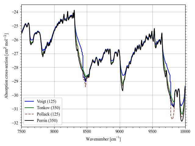
Figure 1: Monochromatic absorption cross-sections of CO₂ at 92.1 bar and 735.3 K as a function of wavenumber in dependence on sub-Lorentzian profile and line-cut condition. Continuum absorption is neglected.

On the fig. 1 we present monochromatic absorption cross-sections calculated with our tool for several line cut conditions and chi-factors. It is similar to the fig. 10 in [4] for better clarity. Some discrepancies could be found in the transparency windows 1.18 and 1.02 $\mu$m due to usage of choice of different spectral database.

4.  Implementation

4.1.  Software design

In developing MARFA, we address the need for more flexible, data-driven, and efficient general-purpose line-by-line tools. Following the surge in popularity of Python within the scientific community, several Python packages have been developed to calculate absorption cross-sections or absorption coefficients, either independently or as part of radiative transfer modeling schemes. Notable examples include HAPI [63], py4Cats [64] (a Python reimplementation of GARLIC [38]), PyRTlib [65], among others. However, our approach offers two modes of interaction: through well-documented Fortran source code and via a web platform that allows users to perform calculations directly. The source codebase might be understood as a “core”, which comprises a line-by-line multi-grid algorithm, basic line shapes, far wings correction functions, line intensity functions, and I/O operations. This “core” is designed to be extensible and reusable under various atmospheric and spectroscopic conditions.

The MARFA project is thoroughly documented to provide quick-start instructions, detailed I/O formats and guidelines for adding custom line shape functions and $\chi$-factors. The codebase employs intuitive variable names, facilitating onboarding of new contributors. Building and running the source code is straightforward using fpm (Fortran Package Manager) [66]. MARFA is designed through Fortran modular structure. This means that each module within the software is dedicated to specific physical or algorithmic operation, such as calculating line shapes, $\chi$-factors, grid calculations, etc. This division to modules enhances the clarity of the code, allowing contributors to focus on individual components without affecting the entire system. Direct access (binary files) format of the output increases the speed of the access to these files for radiative transfer modeling and reduces amount of data post-/pre- processing. Another essential feature of our work is the commitment to the open-source paradigm: the software can be freely contributed to and distributed under provided licenses.

Fortran was chosen as a main programming language of the tool, primarily due to the existence of initial legacy code written in that language. During development and refactoring of the legacy code, we aimed to avoid using outdated features from older versions of Fortran by adhering to the Fortran 2023 standard [67, 68]. However, the module LineGridCalc.f90, containing implementation of the multi-grid interpolation algorithm, still contains legacy features and outdated syntax. In future releases, it is planned to be refactored, although it is isolated and does not compromise the overall clarity and maintainability of the code. Additionally, the MARFA tool may be later converted into a Python package in future, as studies show (e.g. [69]) that NumPy library [70] provides comparable efficiency to Fortran or C/C++ languages.

4.2.  Scope of application and limitations

The codes are particularly well-suited for modeling absorption features in environments where both spectral and atmospheric parameters are uncertain. Our initial focus was made on Venus atmosphere, which explains current absence of predefined atmospheric profiles for other planets. The major scenario targeted by MARFA’s nine-grid interpolation technique involves handling large cut-offs of spectral lines when continuum absorption function is missing. For that reason, currently MARFA does not support the incorporation of continuum absorption.

Only cross-sections or volume absorption coefficients can be calculated when running MARFA. It does not include functionality for modeling instrumental effects, which means that simulated spectra cannot be directly compared with observational data. A fixed resolution of $\approx 5\times 10^{-4}\,\text{cm}^{-1}$ is set, determined by the Doppler half-width in the far-infrared region. Such resolution may be excessive for calculations in the near-infrared region; however, dynamic, user-defined resolutions are planned for future releases. Additionally, while the microwave region can be analyzed with MARFA, specific adjustments, such as Clough correction [71] to the van Vleck-Weisskopf (or van Vleck-Huber) theory [72] and handling “negative wavenumbers”, must be manually applied to ensure accurate calculations.

4.3.  Used data

The tool is designed to minimize the amount of data stored within the project directory, with even fewer datasets embedded directly in the source code. Below, we provide details about the datasets included in the project.

4.3.1.  Spectral Databases

The line-by-line approach requires accessing line data from spectral database files. For cross-section calculations (or absorption coefficients), only the essential (“core”) line parameters are necessary (see, e.g., [64]). To enhance efficiency, the MARFA executable expects these parameters to be stored in a binary file with a specified format. The source code offers built-in functionality to convert standard .par files into a required binary format. For more details, see project documentation.

Spectral databases for the first 12 molecules (based on HITRAN ID), precalculated to the needed format, are available in the data/databases/ directory. These files are generated from .par files from HITRAN 2020. These files might be used for performing immediate calculations or testing. They cover the range from 10 cm^-1. By knowing the required file format (see appendix Appendix B: Utility for processing .par files), users can generate and store their own spectral databases for repeating calculations.

4.3.2.  Total Internal Partition Sums (TIPS)

Partition sums are essential for determining temperature-dependent spectral line intensities. In MARFA, TIPS data are set in an external file and are implemented based on the work of [73]. We introduced only partial data covering the first 74 isotopologues for the first 12 molecules (based on HITRAN ID and isotopologue local ID), over a temperature range of 20–1000 K. The TIPS values for a given isotopologue as a function of temperature can be accessed via the function TIPSofT in the Spectroscopy.f90 module. Future releases will incorporate more recent data from [74], for more broad range of molecules and with considerations for reorganizing the input structure using Fortran subroutine or Python module.

4.3.3.  Molecular Weights

Molecular weights are used for calculating Doppler half-widths and are stored in the MolarMasses.f90 module for the variety of isotopologues.

4.4.  Quick start instructions

The process involves cloning the repository, building the project using the fpm build command, and installing the required Python packages. Predefined atmospheric profiles, such as VenusCO2.dat — which models the CO₂ distribution in Venus’s nightside atmosphere — are available for use. Currently, these profiles are limited to Venus constituents; alternatively, users may create custom atmospheric profiles following the specified format detailed in the project documentation.

Absorption coefficients are computed by executing the fpm run command with command line arguments that include the molecule title, spectral interval, line cut-off condition, atmospheric profile file, and other parameters. Post-processing is performed using a provided Python script that converts output PT-tables into readable formats and generates plots, enabling further spectral analysis such as interval narrowing or resolution enhancement.

4.5.  Adding advanced features and custom line shapes

The MARFA project offers flexibility for users to integrate their own $\chi$-factors and line shape functions, enabling advanced customization of cross-sections calculations. Users can add a custom $\chi$-factor by writing a Fortran function, potentially parameterized by temperature or pressure, and including it within the chiFactors.f90 module. The function must follow the abstract interface for $\chi$-factor functions and be incorporated into the fetchChiFactorFunction() logic.

Custom line shapes can also be introduced by defining new functions in the Shapes module and modifying the logic in the LBL.f90 module to determine their usage across different spectral regions. This allows for non-standard line shapes beyond Voigt, Lorentz, and Doppler models. For more details and examples on integrating custom features, users can refer to the project documentation.

4.6.  Web interface

A web interface has been developed enabling an immediate interaction with MARFA atmospheric absorption calculator. The client side is built using the Next.js framework [75], which supports server-side rendering to ensure quick site loading. On the server side, Django [76] and Django Rest Framework [77] backend frameworks are utilized — a highly scalable and extensible tool-kits, that offer robust built-in database support mechanisms and functionality for building Web APIs. Thus, the client and server communicate through a REST API, enabling fast and seamless data exchange. For the HTTP web server, Nginx [78] is used, while PostgreSQL [79] is used as a primary database for storing information about users requests.

Integration between the backend and MARFA’s Fortran core is achieved by leveraging Django’s ViewSet to invoke external processes via Python’s subprocess module [80]. These processes run fpm executables essential for MARFA’s calculations. Upon completion, the Fortran code generates the resulting PT-tables files, which are stored on the server. After these files are processed, they are provided to the client with download links, allowing users to access their results. The example images  2 and  3 illustrate essential parts of the web interface.

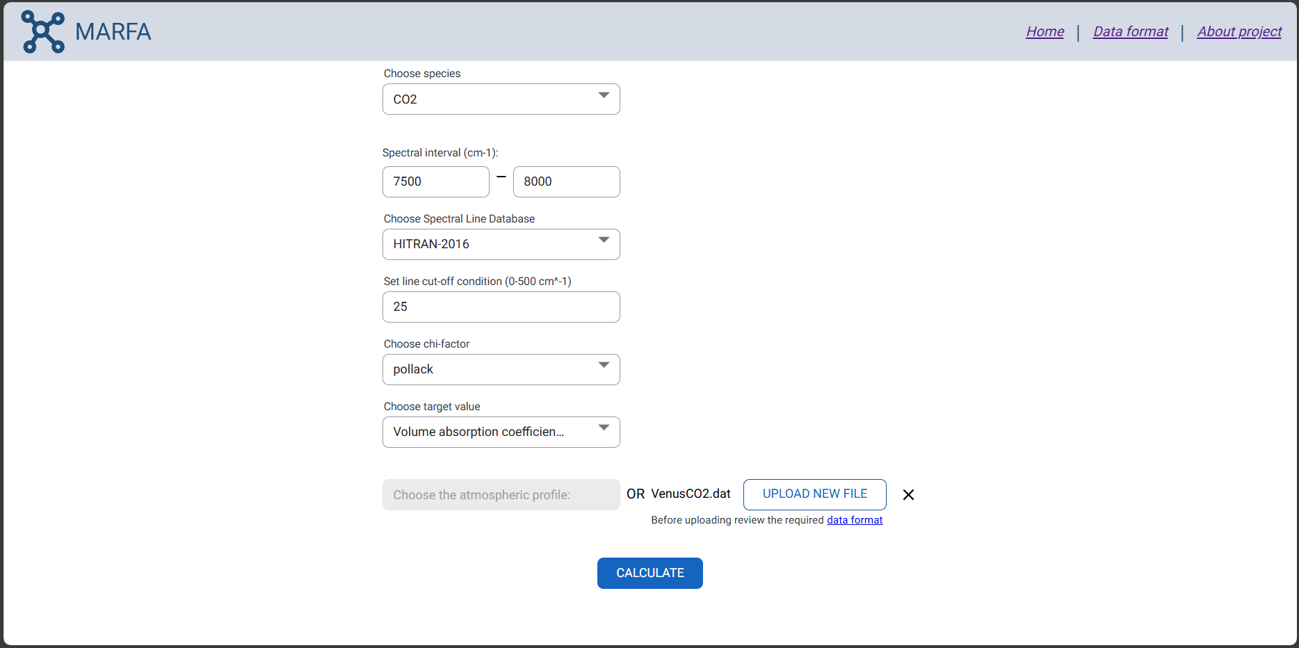
Figure 2: Interface for setting parameters and initiating calculation

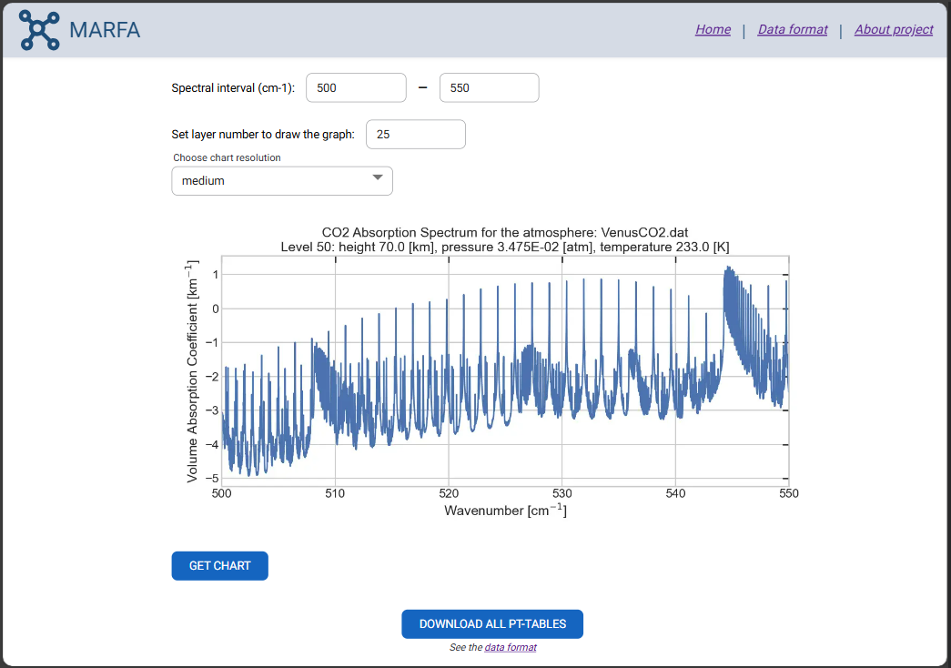
Figure 3: Interface for chart visualization and download options

5.  Conclusion

This paper presents the details of the pre-release version of the MARFA code, designed for calculating molecular absorption cross-sections and volume absorption coefficients for application to planetary atmospheres. Its primary purpose is to equip users with a flexible tool for fast recalculation of absorption signatures under varying atmospheric and spectral scenarios. The source code is available in a public repository, and a web interface has also been developed.

The line-by-line algorithm in MARFA is based on an effective interpolation technique [6], featuring nine uniform grids. It is suitable for scenarios involving large line cut-offs (up to 500 cm^-1). Additionally, MARFA includes clear and detailed documentation, providing a quick start guide and instructions for adding custom features. Output absorption PT-tables can be later directly employed in radiative transfer calculations.

Future releases will focus on introducing parallelization of calculations on different atmospheric levels, adding resolution as an external parameter and bugs fixing. We anticipate that presented tool will be instrumental for atmospheric science researchers in various applications. We are open for any incoming suggestions for future enhancements of this tool.

Appendix A: Structure of the output PT-table file

The output PT-table files are generated and stored within the output/ptTables directory. Each PT-table file is a binary file and corresponds to a specific atmospheric level on which absortption was calculated. File name convention features only the level number, e.g. 1__.ptbin or 65_.ptbin. All the output files have the extension .ptbin.

The structure of the output file is organized into records that contain high-resolution absorption data (direct access file). Each record follows the structure outlined below:

Absorption data and resolution

Each record stores an array, which contains either the cross-section or absorption coefficient data for a specific wavenumber range. Each record corresponds to a 10 cm^-1 interval, controlled by the deltaWV parameter in the source code. The most fine grid in the interpolation technique [6] contains NT = 20481 nodes, thus defining the resolution in the output data:

$$\delta\nu=\frac{\texttt{deltaWV}}{\texttt{NT}}=\frac{10}{20481}\approx 5\times 10^{-4}\,\text{cm}^{-1}$$

Record Indexing

The relationship between a given wavenumber $\nu$ and the record number is defined as:

$$\text{recNum}=\text{int}\left(\frac{\nu}{10}\right)$$

For example, if absorption data for 7564 cm^-1 is required, the corresponding record would be the 756th entry.

Note 1. Current resolution is excessive for mid- and near-IR regions. In future releases, it is planned to increase deltaWV parameter depending on the input interval. There is an opened issue on that topic in the MARFA repository.

Note 2. Record indexing presented above causes an issue that PT-files size depends not only on the spectral interval size, but also on the absolute value of the boundaries. This issue will be resolved in future releases, so the record indexing rule may be changed.

Appendix B: Utility for processing .par files

Absorption signatures are being calculated using a line-by-line approach, which requires spectral database files in a specific format. These files should be placed in the data/databases directory and are typically created based on .par files from sources such as the HITRAN database. These .par files need to be preprocessed into required format before running the main executable. For users convenience, the utility provided in the codebase allows users to perform this preprocessing with simple fpm command, and placing generated files in the target directory.

Database file structure

Each spectral database file is a binary file which is organized as a collection of records (like the output PT-table file). Each record corresponds to one spectral line and contain its “core” parameters. The parameters include (for more details for each item, see [22]):

1. the wavenumber of the transition ($\nu_{ij}$) in double precision

2. the spectral line intensity ($S_{ij}$) at 296 K

3. the air-broadened half width at half maximum (HWHM) at 296 K ($\gamma_{\text{air}}$)

4. the self-broadened half width at half maximum (HWHM) at 296 K ($\gamma_{\text{self}}$)

5. the lower-state energy of the transition ($E^{\prime\prime}$)

6. the coefficient of the temperature dependence of the air-broadened half width ($n_{\text{air}}$)

7. jointMolIso - custom parameter, which contains information on both molecule id (Mol) and isotopologue id (Iso). For more details, refer to the documentation.

8. the pressure shift at 296 K and 1 atm of the line position with respect to the vacuum transition wavenumber ($\delta_{\text{air}}$)

Since there are 8 parameters and for storing one 8 bytes are needed, the total record length equals to 36 bytes. This standardized structure ensures that all necessary parameters are available and improves speed of line-by-line absorption calculations.

References

- [1] S. Drayson “Atmospheric Transmission in the CO2 Bands Between 12 and 18” In Appl. Opt. 5, 1966, pp. 385 DOI: 10.1364/AO.5.000385
- [2] Shepard A Clough, Michael J Iacono and Jean-Luc Moncet “Line-by-line calculations of atmospheric fluxes and cooling rates: Application to water vapor” In Journal of Geophysical Research: Atmospheres 97.D14 Wiley Online Library, 1992, pp. 15761–15785
- [3] S.. Clough et al. “Atmospheric radiative transfer modeling: A summary of the AER codes” In Journal of Quantitative Spectroscopy and Radiative Transfer 91, 2005, pp. 233–244 DOI: 10.1016/j.jqsrt.2004.05.058
- [4] Rainer Haus and Gabriele Arnold “Radiative transfer in the atmosphere of Venus and application to surface emissivity retrieval from VIRTIS/VEX measurements” In Planetary and Space Science 58 Elsevier, 2010, pp. 1578–1598 DOI: 10.1016/j.pss.2010.08.001
- [5] R. Haus, D. Kappel and G. Arnold “Radiative heating and cooling in the middle and lower atmosphere of Venus and responses to atmospheric and spectroscopic parameter variations” In Planetary and Space Science 117 Elsevier, 2015, pp. 262–294 DOI: 10.1016/j.pss.2015.06.024
- [6] B.A. Fomin “Effective interpolation technique for line-by-line calculations of radiation absorption in gases” In Journal of Quantitative Spectroscopy and Radiative Transfer 53.6 Elsevier, 1995, pp. 663–669
- [7] Martin Kuntz and Michael Höpfner “Efficient line-by-line calculation of absorption coefficients” In Radiative Transfer 63, 1999, pp. 97–114
- [8] B.. Fomin “Efficient line-by-line technique for calculating accurate and compact spectral lookup tables for satellite remote sensing” In International Journal of Remote Sensing 42 TaylorFrancis Ltd., 2020, pp. 3074–3089 DOI: 10.1080/01431161.2020.1865586
- [9] Josef Humlíček “Optimized computation of the Voigt and complex probability functions” In Journal of Quantitative Spectroscopy and Radiative Transfer 27.4 Elsevier, 1982, pp. 437–444
- [10] H. Tran, N.. Ngo and J.. Hartmann “Efficient computation of some speed-dependent isolated line profiles” In Journal of Quantitative Spectroscopy and Radiative Transfer 129, 2013, pp. 199–203 DOI: 10.1016/j.jqsrt.2013.06.015
- [11] N.. Ngo, D. Lisak, H. Tran and J.. Hartmann “An isolated line-shape model to go beyond the Voigt profile in spectroscopic databases and radiative transfer codes” In Journal of Quantitative Spectroscopy and Radiative Transfer 129, 2013, pp. 89–100 DOI: 10.1016/j.jqsrt.2013.05.034
- [12] PW Rosenkranz “Pressure broadening of rotational bands. I. A statistical theory” In The Journal of chemical physics 83.12 AIP Publishing, 1985, pp. 6139–6144
- [13] Philip L. Varghese and Ronald K. Hanson “Collisional narrowing effects on spectral line shapes measured at high resolution” In Applied Optics 23, 1984, pp. 2376–2385
- [14] Darrell E. Burch, David A. Gryvnak, Richard R. Patty and Charlotte E Bartky “Absorption of infrared radiant energy by CO2 and H2O. IV. Shapes of collision-broadened CO2 lines” In JOSA 59.3 Optica Publishing Group, 1969, pp. 267–280
- [15] James B. Pollack et al. “Near-Infrared Light from Venus’ Nightside: A Spectroscopic Analysis” In Icarus 103, 1993, pp. 1–42 DOI: 10.1006/icar.1993.1055
- [16] MV Tonkov et al. “Measurements and empirical modeling of pure CO2 absorption in the 2.3-m region at room temperature: far wings, allowed and collision-induced bands” In Applied optics 35.24 Optica Publishing Group, 1996, pp. 4863–4870
- [17] RM Goody and YL Yung “Atmospheric Radiation: Theoretical Basis” Oxford University Press, 1989
- [18] I.. Gordon et al. “The HITRAN2020 molecular spectroscopic database” In Journal of Quantitative Spectroscopy and Radiative Transfer 277 Elsevier Ltd, 2022 DOI: 10.1016/j.jqsrt.2021.107949
- [19] I.. Gordon et al. “The HITRAN2016 molecular spectroscopic database” In Journal of Quantitative Spectroscopy and Radiative Transfer 203 Elsevier Ltd, 2017, pp. 3–69 DOI: 10.1016/j.jqsrt.2017.06.038
- [20] Nicole Jacquinet-Husson et al. “The 2003 edition of the GEISA/IASI spectroscopic database” In Journal of Quantitative Spectroscopy and Radiative Transfer 95, 2005, pp. 429–467 DOI: 10.1016/j.jqsrt.2004.12.004
- [21] N. Jacquinet-Husson et al. “The GEISA spectroscopic database: Current and future archive for Earth and planetary atmosphere studies” In Journal of Quantitative Spectroscopy and Radiative Transfer 109, 2008, pp. 1043–1059 DOI: 10.1016/j.jqsrt.2007.12.015
- [22] HITRAN Database “Definitions and Units for HITRAN Data” Accessed: October 29, 2024, https://hitran.org/docs/definitions-and-units/, 2024
- [23] BH Armstrong “Spectrum line profiles: the Voigt function” In Journal of Quantitative Spectroscopy and Radiative Transfer 7.1 Elsevier, 1967, pp. 61–88
- [24] M. Kuntz “A new implementation of the Humlicek algorithm for the calculation of the Voigt profile function” In Journal of Quantitative Spectroscopy and Radiative Transfer 57.6 Elsevier, 1997, pp. 819–824
- [25] Lazaros Oreopoulos et al. “The continual intercomparison of radiation codes: Results from phase I” In Journal of Geophysical Research: Atmospheres 117.D6 Wiley Online Library, 2012
- [26] Rangasayi N Halthore et al. “Intercomparison of shortwave radiative transfer codes and measurements” In Journal of Geophysical Research: Atmospheres 110.D11 Wiley Online Library, 2005
- [27] MY Perrin and JM Hartmann “Temperature-dependent measurements and modeling of absorption by CO2-N2 mixtures in the far line-wings of the 4.3 m CO2 band” In Journal of Quantitative Spectroscopy and Radiative Transfer 42.4 Elsevier, 1989, pp. 311–317
- [28] SA Clough, FX Kneizys and RW Davies “Line Shape and the Water Vapor Continuum” In Atmospheric Research 23, 1989, pp. 229–241
- [29] DP Edwards “Atmospheric transmittance and radiance calculations using line-by-line computer models” In Proceedings of SPIE, 1988, pp. 94–116 DOI: 10.1117/12.975622
- [30] Robert West, David Crisp and Luke Chen “Mapping transformations for broadband atmospheric radiation calculations” In Journal of Quantitative Spectroscopy and Radiative Transfer 43.3 Elsevier, 1990, pp. 191–199
- [31] Larry L. Gordley, Benjamin T. Marshall and D. Chu “LINEPAK: Algorithms for Modeling Spectral Transmittance and Radiance” In J. Quant. Spectrosc. Radiat. Tramfer 52, 1994, pp. 563–580
- [32] Lawrence Sparks “Efficient line-by-line calculation of absorption coefficients to high numerical accuracy” In Journal of Quantitative Spectroscopy and Radiative Transfer 57.5 Elsevier, 1997, pp. 631–650
- [33] DV Titov and Rainer Haus “A fast and accurate method of calculation of gaseous transmission functions in planetary atmospheres” In Planetary and space science 45.3 Elsevier, 1997, pp. 369–377
- [34] Michel Kruglanski and Martine De Maziere “Fast method for calculating infrared spectral transmittances in the wings of absorption lines” In Journal of quantitative spectroscopy and radiative transfer 94.1 Elsevier, 2005, pp. 117–125
- [35] Franz Schreier “Optimized evaluation of a large sum of functions using a three-grid approach” In Computer Physics Communications 174, 2006, pp. 783–792 DOI: 10.1016/j.cpc.2005.12.015
- [36] Shepard A. Clough and Francis X. Kneizys “Convolution algorithm for the Lorentz function” In Applied Optics 18.13 Optica Publishing Group, 1979, pp. 2329–2333
- [37] SA Clough, FX Kneizys, LS Rothman and WO Gallery “Atmospheric spectral transmittance and radiance: FASCOD1 B” In Atmospheric transmission 277, 1981, pp. 152–167 SPIE
- [38] Franz Schreier et al. “GARLIC - A general purpose atmospheric radiative transfer line-by-line infrared-microwave code: Implementation and evaluation” In Journal of Quantitative Spectroscopy and Radiative Transfer 137 Elsevier Ltd, 2014, pp. 29–50 DOI: 10.1016/j.jqsrt.2013.11.018
- [39] Boris Fomin and Mikhail Razumovskiy “Effective parameterization of absorption by gaseous species and unknown UV absorber in 125–400 nm region of Venus atmosphere” In Journal of Quantitative Spectroscopy and Radiative Transfer 286 Elsevier Ltd, 2022, pp. 108201 DOI: 10.1016/j.jqsrt.2022.108201
- [40] D. Ehrenreich et al. “Transmission spectrum of Venus as a transiting exoplanet” In Astronomy and Astrophysics 537, 2012 DOI: 10.1051/0004-6361/201118400
- [41] Laura Schaefer and Bruce Fegley “Atmospheric chemistry of VENUS-like exoplanets” In Astrophysical Journal 729 Institute of Physics Publishing, 2011 DOI: 10.1088/0004-637X/729/1/6
- [42] L.. Zasova et al. “Structure of the Venusian atmosphere from surface up to 100 km” In Cosmic Research 44.4, 2006, pp. 364–383 DOI: 10.1134/S0010952506040095
- [43] A. Seiff et al. “Models of the structure of the atmosphere of Venus from the surface to 100 kilometers altitude” In Advances in Space Research 5, 1985, pp. 3–58 DOI: 10.1016/0273-1177(85)90197-8
- [44] GM Keating, JY Nicholson III and LR Lake “Venus upper atmosphere structure” In Journal of Geophysical Research: Space Physics 85.A13 Wiley Online Library, 1980, pp. 7941–7956
- [45] GM Keating et al. “Models of Venus neutral upper atmosphere: Structure and composition” In Advances in Space Research 5.11 Elsevier, 1985, pp. 117–171
- [46] A Seiff and Donn B Kirk “Structure of the Venus mesosphere and lower thermosphere from measurements during entry of the Pioneer Venus probes” In Icarus 49.1 Elsevier, 1982, pp. 49–70
- [47] Constantine C.C. Tsang et al. “Tropospheric carbon monoxide concentrations and variability on Venus from Venus Express/VIRTIS-M observations” In Journal of Geophysical Research E: Planets 114.5, 2009, pp. 1–13 DOI: 10.1029/2008JE003089
- [48] Rainer Haus, David Kappel and Gabriele Arnold “Self-consistent retrieval of temperature profiles and cloud structure in the northern hemisphere of Venus using VIRTIS/VEX and PMV/VENERA-15 radiation measurements” In Planetary and Space Science 89 Elsevier, 2013, pp. 77–101
- [49] C..C. Tsang, P..J. Irwin, F.. Taylor and C.. Wilson “A correlated-k model of radiative transfer in the near-infrared windows of Venus” In Journal of Quantitative Spectroscopy and Radiative Transfer 109.6, 2008, pp. 1118–1135 DOI: 10.1016/j.jqsrt.2007.12.008
- [50] Laurence S Rothman et al. “The HITRAN 2004 molecular spectroscopic database” In Journal of quantitative spectroscopy and radiative transfer 96.2 Elsevier, 2005, pp. 139–204
- [51] Laurence S Rothman et al. “The HITRAN 2008 molecular spectroscopic database” In Journal of Quantitative Spectroscopy and Radiative Transfer 110.9-10 Elsevier, 2009, pp. 533–572
- [52] L.. Rothman et al. “The HITRAN2012 molecular spectroscopic database” In Journal of Quantitative Spectroscopy and Radiative Transfer 130, 2013, pp. 4–50 DOI: 10.1016/j.jqsrt.2013.07.002
- [53] Laurence S Rothman et al. “HITRAN HAWKS and HITEMP: high-temperature molecular database” In Atmospheric Propagation and Remote Sensing IV 2471 International Society for Optical Engineering (SPIE Proceedings, Vol. 2471), 1995, pp. 105–111
- [54] L.. Rothman et al. “HITEMP, the high-temperature molecular spectroscopic database” In Journal of Quantitative Spectroscopy and Radiative Transfer 111, 2010, pp. 2139–2150 DOI: 10.1016/j.jqsrt.2010.05.001
- [55] Sergey A. Tashkun et al. “CDSD-1000, the high-temperature carbon dioxide spectroscopic databank” In Journal of Quantitative Spectroscopy and Radiative Transfer 82.1-4 Elsevier, 2003, pp. 165–196
- [56] David Kappel et al. “Refinements in the data analysis of VIRTIS-M-IR Venus nightside spectra” In Advances in Space Research 50 Elsevier Ltd, 2012, pp. 228–255 DOI: 10.1016/j.asr.2012.03.029
- [57] David Kappel, Gabriele Arnold and Rainer Haus “Multi-spectrum retrieval of Venus IR surface emissivity maps from VIRTIS/VEX nightside measurements at Themis Regio” In Icarus 265 Academic Press Inc., 2016, pp. 42–62 DOI: 10.1016/j.icarus.2015.10.014
- [58] Bruno Bezard et al. “Water vapor abundance near the surface of Venus from Venus Express/VIRTIS observations” In Journal of Geophysical Research: Planets 114 American Geophysical Union, 2009 DOI: 10.1029/2008JE003251
- [59] Bruno Bézard et al. “The 1.10- and 1.18-m nightside windows of Venus observed by SPICAV-IR aboard Venus Express” In Icarus 216, 2011, pp. 173–183 DOI: 10.1016/j.icarus.2011.08.025
- [60] M Fukabori, T Nakazawa and M Tanaka “Absorption properties of infrared active gases at high pressures—I. CO2” In Journal of Quantitative Spectroscopy and Radiative Transfer 36.3 Elsevier, 1986, pp. 265–270
- [61] Bruno Bézard, Catherine De Bergh, David Crisp and Jean-pierre Maillard “The deep atmosphere of Venus revealed by high-resolution nightside spectra” In Nature 345.6275 Nature Publishing Group UK London, 1990, pp. 508–511
- [62] Bruno Bézard et al. “Water vapor abundance near the surface of Venus from Venus Express/VIRTIS observations” In Journal of Geophysical Research: Planets 114.E5 Wiley Online Library, 2009
- [63] Roman V Kochanov et al. “HITRAN Application Programming Interface (HAPI): A comprehensive approach to working with spectroscopic data” In Journal of Quantitative Spectroscopy and Radiative Transfer 177 Elsevier, 2016, pp. 15–30
- [64] Franz Schreier, Sebastián Gimeno García, Philipp Hochstaffl and Steffen Städt “Py4cats—PYthon for computational ATmospheric spectroscopy” In Atmosphere 10.5 MDPI, 2019, pp. 262
- [65] Salvatore Larosa et al. “PyRTlib: an educational Python-based library for non-scattering atmospheric microwave radiative transfer computations” In Geoscientific Model Development 17.5 Copernicus Publications Göttingen, Germany, 2024, pp. 2053–2076
- [66] Fortran-lang Contributors “fpm: Fortran Package Manager” Accessed: 2024-04-27, https://fortran-lang.org/fpm/, 2024
- [67] Michael Metcalf, John Reid, Malcolm Cohen and Reinhold Bader “Modern Fortran Explained: Incorporating Fortran 2023” Oxford University Press, 2024
- [68] ISO/IEC JTC1/SC22/WG5 “Fortran 2023 standard” Accessed: 2024-04-27, https://wg5-fortran.org/f2023.html, 2023
- [69] Franz Schreier “The Voigt and complex error function: Humlíček’s rational approximation generalized” In Monthly Notices of the Royal Astronomical Society 479.3 Oxford University Press, 2018, pp. 3068–3075
- [70] Charles R Harris et al. “Array programming with NumPy” In Nature 585.7825 Nature Publishing Group UK London, 2020, pp. 357–362
- [71] SA Clough et al. “Atmospheric Water Vapor, chapter 2” Acedemic Press, Inc, 1980
- [72] J.. Vleck and D.. Huber “Absorption, emission, and linebreadths: A semihistorical perspective” In Reviews of Modern Physics 49, 1977, pp. 939–959 DOI: 10.1103/RevModPhys.49.939
- [73] Robert R. Gamache, Michaella Farese and Candice L. Renaud “A spectral line list for water isotopologues in the 1100-4100 cm-1 region for application to CO2-rich planetary atmospheres” In Journal of Molecular Spectroscopy 326 Academic Press Inc., 2016, pp. 144–150 DOI: 10.1016/j.jms.2015.09.001
- [74] Robert R. Gamache et al. “Total internal partition sums for the HITRAN2020 database” In Journal of Quantitative Spectroscopy and Radiative Transfer 271 Elsevier Ltd, 2021 DOI: 10.1016/j.jqsrt.2021.107713
- [75] Vercel “Next.js” Accessed: October 29, 2024, https://nextjs.org/, 2024
- [76] Django Software Foundation “Django” Accessed: October 29, 2024, https://www.djangoproject.com/, 2024
- [77] Tom Christie “Django REST Framework” Accessed: October 29, 2024, https://www.django-rest-framework.org/, 2024
- [78] Igor Sysoev and Inc. Nginx “Nginx: A High-Performance Web Server and Reverse Proxy Server” Accessed: October 29, 2024, https://nginx.org/, 2024
- [79] PostgreSQL Global Development Group “PostgreSQL: The World’s Most Advanced Open Source Relational Database” Accessed: October 29, 2024, https://www.postgresql.org/, 2024
- [80] Python Software Foundation “subprocess — Subprocess management” Accessed: October 29, 2024, 2024 Python URL: https://docs.python.org/3/library/subprocess.html