Accelerating Gaussian Variational Inference for Motion Planning Under Uncertainty
Abstract
This work addresses motion planning under uncertainty as a stochastic optimal control problem. The path distribution induced by the optimal controller corresponds to a posterior path distribution with a known form. To approximate this posterior, we frame an optimization problem in the space of Gaussian distributions, which aligns with the Gaussian Variational Inference Motion Planning (GVIMP) paradigm introduced in [1]. In this framework, the computation bottleneck lies in evaluating the expectation of collision costs over a dense discretized trajectory and computing the marginal covariances. This work exploits the sparse motion planning factor graph, which allows for parallel computing collision costs and Gaussian Belief Propagation (GBP) marginal covariance computation, to introduce a computationally efficient approach to solving GVIMP. We term the novel paradigm as the Parallel Gaussian Variational Inference Motion Planning (P-GVIMP). We validate the proposed framework on various robotic systems, demonstrating significant speed acceleration achieved by leveraging Graphics Processing Units (GPUs) for parallel computation. An open-sourced implementation is presented at https://github.com/hzyu17/VIMP.
I Introduction
Motion Planning is one core decision-making component in autonomous robotic systems [2, 3]. Given an environment, a start configuration, and a goal configuration, a motion planner computes a trajectory connecting the two configurations. The trajectory optimization paradigm [4, 5] formulates the motion planning problem as an optimization over all admissible trajectories with dynamics and environment constraints. An ‘optimal’ plan can be obtained by solving the optimization program by minimizing certain optimality indexes, such as time consumption, control energy, and safety.
In real-world scenarios, uncertainties such as modeling and actuation noises and external disturbances arise and affect the quality of the motion plans in the execution phase. To reduce its impacts, motion planning under uncertainties takes into account the uncertainties in the planning phase in their formulations [6]. Stochastic optimal control and probabilistic robotics [7, 8] provide a principled framework to address this problem, where noises are explicitly modeled in the robots’ dynamics, and the optimality index is converted into a statistical one over the trajectory distribution space.
In this work, the uncertainties are modeled as Wiener processes injected into linear dynamics. The resulting underlying robot dynamics are linear Stochastic Differential Equations (SDEs) [9]. Gaussian Process Motion Planning (GPMP) paradigm [10, 11] leveraged this dynamic model in the motion planning problems. With this formulation, the deterministic trajectory optimization with collision-avoiding constraints becomes a probabilistic one, and the optimal motion plan can be written as a posterior probability. The objective in GPMP is solving a trajectory that maximizes this posterior probability, turning trajectory optimization into a probability inference problem.
The solution obtained from GPMP is still a deterministic trajectory. Leveraging planning-as-inference dual formulation, more comprehensive statistical methods can be applied to solve motion planning problems. Variational Inference [12, 13] formulates the inference problem into an optimization within a parameterized proposal distribution family. The solution is an optimized proposal distribution close to the posterior measured by the Kullback–Leibler (KL) divergence. VI can be applied to solve for a trajectory distribution in the planning-as-inference formulation [14, 15, 1, 16, 17]. The resulting trajectory distribution [1] showed satisfying performances in challenging tasks such as planning through a narrow gap [18], and this formulation is naturally connected to entropy-regularized robust motion planning [19, 20, 21].
Introducing distributional variables increases the dimension of the problem. The joint covariance over the whole trajectory is quadratic in the trajectory length. Fortunately, in motion planning problems, the underlying probabilistic graph enjoys a sparsity pattern [22], which can be leveraged to factorize the target posterior and reduce the number of variational variables [23, 21]. In this work, we further leverage this sparse factor and the parallel computing on GPUs to accelerate the computation of two key components in the GVI motion planning paradigm: the parallel computation of the collision likelihood and the computation of marginal covariances over the sparse factor graph.
The variational inference over trajectory distributions is dual to stochastic optimal control problem for the same Gaussian process dynamics, which is the special case of the duality between probability graph inference and optimal control [24, 25, 19, 20] when the dynamics are linear Gaussian [21]. In this work, we start from a stochastic control formulation to obtain the target posterior distribution in GPMP for the nonlinear motion planning problems for Gaussian processes. This posterior is the distribution induced by the optimal solution controller. GVIMP is an approximate inference approach [26] to optimal path distribution in the Gaussian distribution space.
II Notations and Preliminaries
II-A Planning under Uncertainties as Stochastic Control
We solve the motion planning under uncertainties using the stochastic control framework. Consider affine time-varying stochastic system
| (1) |
For the system (1), we minimize the following objective
| (2) |
where we have a running cost consisting of a state-related running cost , and the control energy , and is a terminal cost. The state costs regulate the desired behaviors, such as collision avoidance. Controlling energy costs promotes a minimum energy consumption strategy for the robot to achieve the above goals.
II-B Linear Gaussian Markov Process
The prior process associated with the process (1) is defined by letting , resulting in the process
| (3) |
We introduce the time discretization scheme
| (4) |
which generates a vector of discretized states and control inputs of length . The support states and the support controls over this time discretization are denoted as
| (5) |
where
The covariance matrix of is denoted as . The joint Gaussian trajectory prior distribution is
| (6) |
The state transition kernel of the linear system (1) from time to is denoted as which satisfies for all
The Grammian associated with the system (1) is
| (7) |
II-C Variational Inference and ELBO
Variational Inference (VI) is a technique for approximating an intractable probability distribution by approximating it with another distribution in a tractable distribution family. For a target distribution , VI solves a distribution by minimizing the Kullback-Leibler (KL) divergence
| (8) |
The target distribution is unknown in general. One particular common situation is that the target distribution is only known up to a normalizing constant, , i.e.,
| (9) |
The normalizing constant is often hard to compute directly. Starting from the definition of the KL-divergence between two distributions, we have
| (10) |
Define the KL-divergence between the proposal and the un-normalized target as , i.e.,
then we have
| (11) |
Thus, is a lower bound of the original objective in (8). This famous lower bound is known as the Evidence Lower Bound (ELBO) [27]. Starting from (11), Variational Inference maximizes the ELBO in order to minimize the original intractable KL-divergence (8), which yields
| (12) |
III Problem Statement
III-A Path Distribution Control with Nonlinear State Costs.
The control problem (2) can be re-formulated into an equivalent path distribution control problem. Denote the measure induced by the controlled process (1) as , and the measure induced by the prior process (3) as . The special term on control energy cost in (2) can be leveraged to transform the problem into a distributional control. By Girsanov’s theorem [28], the expected control energy equals to the relative entropy between and , i.e.,
| (13) |
leading to the following equivalent objective function to (2)
| (14) |
where
and the measure is defined as
| (15) |
Discrete-Time Formulation. Consider the above KL-minimization problem (8) with the time discretization in (4). For the linear Gaussian prior dynamics (3), the discrete-time path distribution over is exactly the joint Gaussian distribution defined in (6). i.e.,
The discrete-time cost factor is
then the discrete-time optimal distribution to the problem (8) is defined as the following joint distribution over
| (16) |
This optimal distribution is exactly the posterior distribution in the GPMP formulation [10, 21].
III-B Gaussian Variational Inference Motion Planning (GVI-MP)
We just showed that for the stochastic control problem (2), the path distribution under the optimal controller is known up to a normalizing constant as as defined in (16). This form is familiar in the Variational Inference problem formulation (9) in the path distribution space. The path space Variational Inference problem is formulated as
| (17) | ||||
where consists of the parameterized proposal Gaussian distributions.
Natural gradient descent is a classical algorithm for solving the Gaussian Variational Inference problem. Define the negative log probability for the posterior as . The Variational Inference objective is equivalent to
where denotes the entropy of the distribution , which promotes the robustness of the motion plan solution. We add an additional temperature parameter, , to trade off this robustness, leading to the objective of temperature
| (18) |
We parameterize the proposed Gaussian using its mean and inverse of covariance . The derivatives with respect to and are [29]
| (19a) | ||||
| (19b) | ||||
Natural gradient descent update w.r.t. objective is
| (20) |
IV Parallel GVI Motion Planning
The computation bottleneck of the natural gradient paradigm in GVIMP is evaluating the nonlinear collision costs and computing marginal covariance matrices. This section introduces a parallel paradigm for the above two computations: the Parallel Gaussian Variational Inference Motion Planning (P-GVIMP).
IV-A Parallel Computation of Collision Cost Factors
The joint precision matrix has a sparsity structure [10]
| (23) |
and
| (24) |
where are desired start and goal states covariances. For a controllable system, the Grammian (7) is invertible.
Given the sparsity (23) and (24), denote the deviated states as and the prior and collision costs as respectively. We have then
where the factorized potentials are defined as
The factor-level Gaussian variables are linearly mapped from the joint variables
| (27) |
The resulting motion planning factor graph is showned in the following Fig. 1.
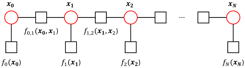
With the factorization (27), we observe that the joint collision costs is decomposed into individual factors on the marginal Gaussians . This factorized structure can be leveraged to distribute the computation of on a GPU.
IV-B Belief Propagation for Marginal Covariances Update
Another major bottleneck in computation is computing the marginal covariances. A brute force inverse computation of the joint covariance from has the complexity , which is a cubic function in in motion planning. Leveraging the sparse factor graph, this section leverages the Gaussian Belief Propagation (GBP) [30, 31] to compute the marginals over the factor graph. Gaussian distribution can be written in the canonical form
| (28) |
where denotes the precision matrix, and denotes the information vector
To simplify the computation, we can assume a shifted Gaussian distribution , since we only want to obtain the marginal covariance. Then can be written as
| (29) |
The precision matrix has such sparsity pattern
| (30) |
and the Gaussian distribution (29) can be factorized into
| (31) |
with
and
Gaussian Belief Propagation is an algorithm for calculating the marginals of a joint distribution via local message passing between nodes in a factor graph [31]. Since all of these factors are Gaussian, we can use this method directly.
Message passing on the factor graph can be divided into two types. The message passed from variables to factors, denoted as , and the message passed from factors to variables, denoted as . Messages can be obtained by
| (32a) | |||||
| (32b) | |||||
where denotes all the neighboring factors of , denotes the factor potential of the factor .
After computing all the messages in the factor graph, the beliefs of variables can be obtained by taking the product of incoming messages:
| (33) |
since the messages here are also Gaussian distribution, we can obtain the belief parameters :
| (34) |
The time complexity of inverting a matrix is , leading to a total complexity for GBP.
IV-C Parallel GVIMP Algorithm
This section presents the Parallel GVIMP algorithm on LTV stochastic dynamical systems from the linearization of the system (37) and performs a Parallel GVIMP on the obtained linearized LTV system to get the optimized nominal mean and covariance trajectories. The algorithm is summarized in the following Algorithm 1. This algorithm can serve as a module in planning non-linear systems by iterative linearization [32, 21]. We also introduce Exponential Moving Average (EMA) updates, which empirically further smooth the trajectories obtained at each iteration. For the trajectory mean and precision at iteration , the EMA update equations are as follows:
| (35) | ||||
where is a smoothing factor.
| Prior | Collision | MP | Entropy | Total | |
|---|---|---|---|---|---|
| Go Through | 94.085 | 0.6046 | 94.689 | 539.272 | 633.961 |
| Go Around | 109.163 | 0.4129 | 109.576 | 472.852 | 586.428 |
IV-D Complexity Analysis
We now analyze the time complexity of the proposed decentralized algorithm. The state dimension is , and time discretization is . The factor graph has factors, the maximum dimension being . A serial computation of the nonlinear factor computations leads to a linear dependence on , and the total complexity is , where is the precision required in the GH-quadrature [21]. Experimentally, to obtain a precise estimate of the collision costs, . The parallel nonlinear factor computation is of complexity , and the complexity of computing the marginal covariances for the tree-structured factor graph using GBP is of . The overall complexity of the algorithm is therefore reduced from to , which is not dependent on the quadrature precision .
| D Point Robot | D Point Robot | |
|---|---|---|
| Brute force inverse | ms | ms |
| GBP | ms | ms |
| Improvement | 60.08 % | 75.80 % |
V experiments
This section shows the results of the numerical experiments for the proposed method.
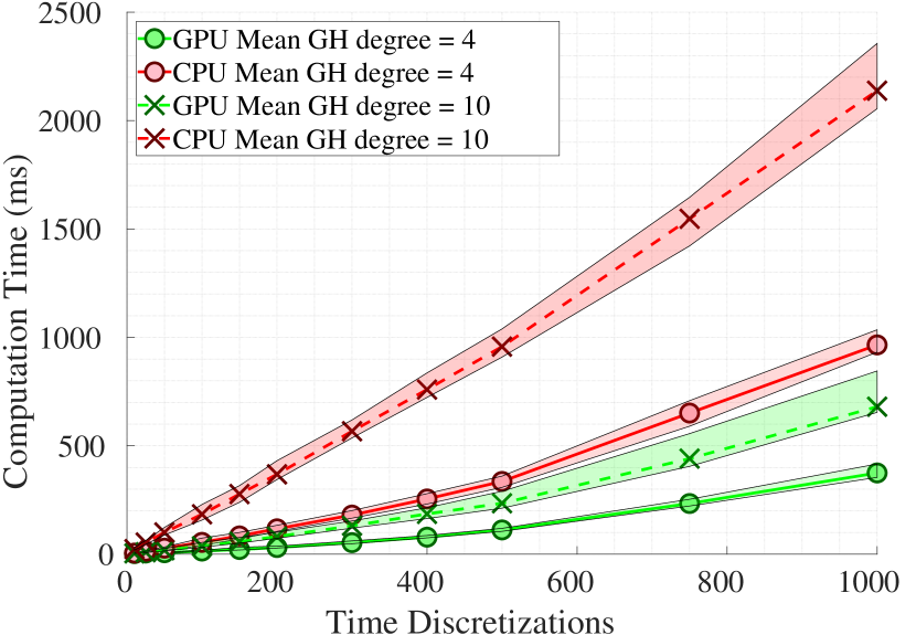
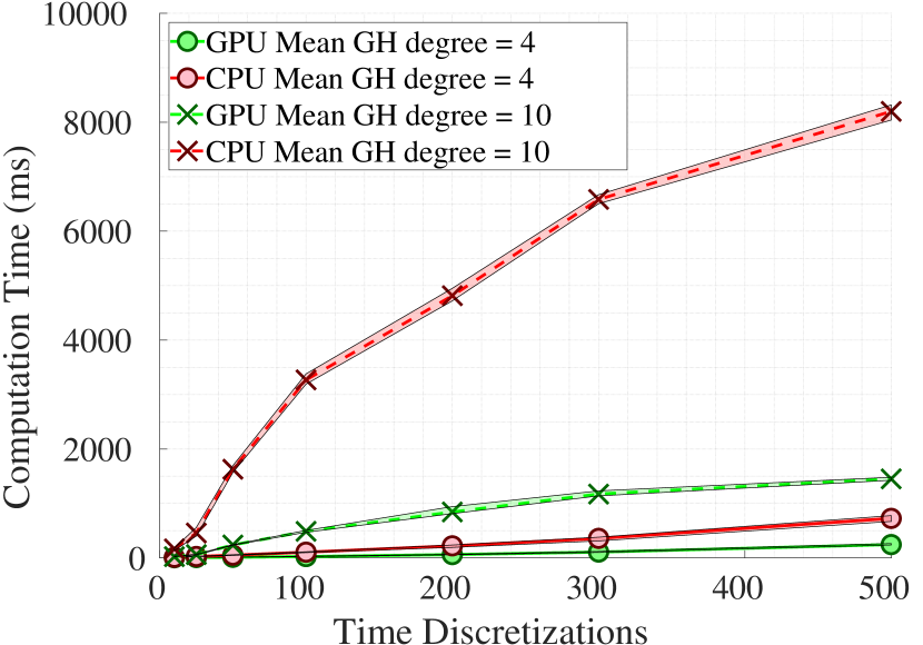
V-A Efficiency Improvement through Distributed Computation
We first compare the time of computing the expected collision factors between the GPU distributed method proposed in this work and a serial implementation. We made the comparison on D and D point robots with linear time-invarying (LTI) stochastic system
| (36) |
The results are shown in Tab. III.
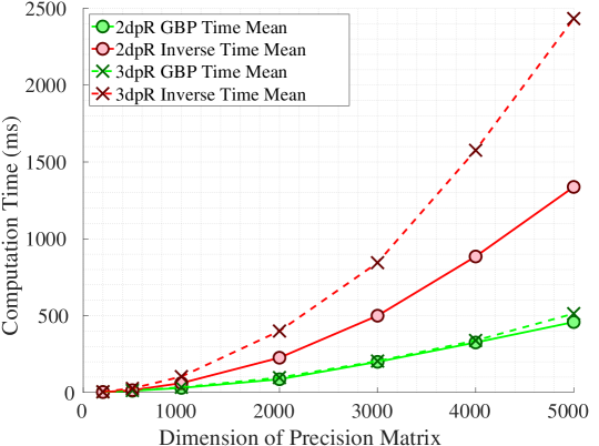
Next, we do comparison studies on computing the inverse of the precision matrix, , using a direct matrix inversion versus using GBP proposed in this work. The comparison results are in the Tab. II and Fig. 5. We see a linear dependence on the number of time discretizations for GBP, and a polynomial () dependence of direct inversion. For , a improvement in implementation time is gained through GBP for point robot.
| D Point Robot | D Point Robot | |
|---|---|---|
| Serial | ms | ms |
| Parallel | ms | ms |
| Improvement | 80.12 % | 85.05 % |
| D Point Robot | D Point Robot | |
|---|---|---|
| Serial | s | s |
| Parallel | s | s |
| Improvement | 70.29 % | 79.97 % |
V-B P-GVIMP for LTV Systems
Next, we validate our proposed algorithm on a planar quadrotor system defined as
| (37) |
where is the gravity, represents the mass of the planar quadrotor, is the length of the body, and is the moment of inertia. and are the two thrust inputs to the system. In all our experiments, we set , and .
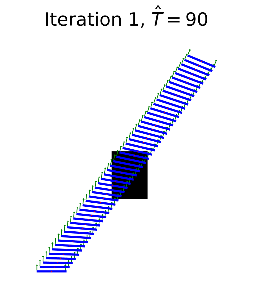
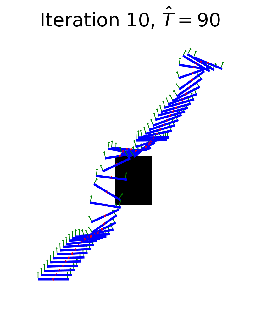
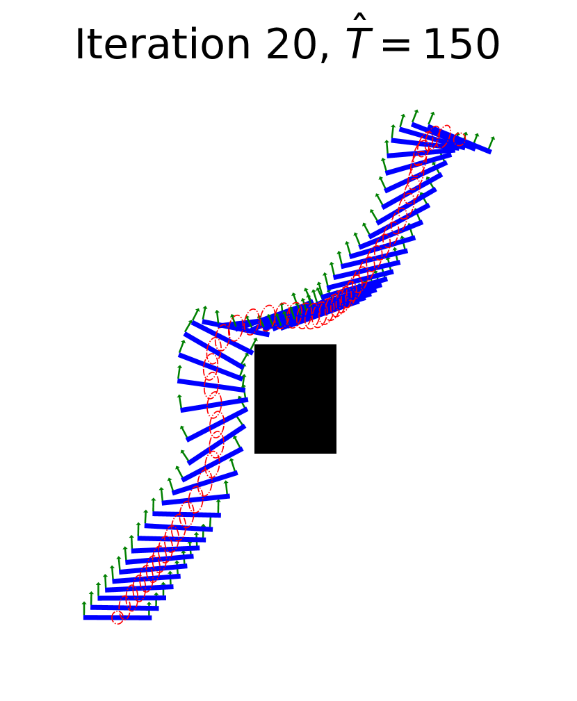
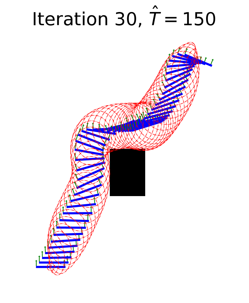
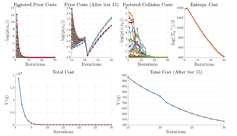
(a) Convergence for LTV system. We show the convergence of the algorithm via a downsampled plot of the intermediate proposal Gaussian trajectory distributions in Fig. 3 with the low and high temperatures in (18), and the corresponding cost evolutions, both for prior and collision factorized costs, and the total cost, in Fig. 4. After obtaining a collision-free trajectory with low temperatures, we switched to a high-temperature phase to put more weight on the entropy costs. The total costs keep decreasing throughout both processes.
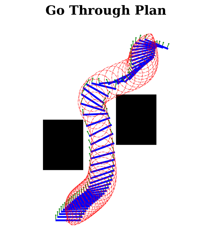
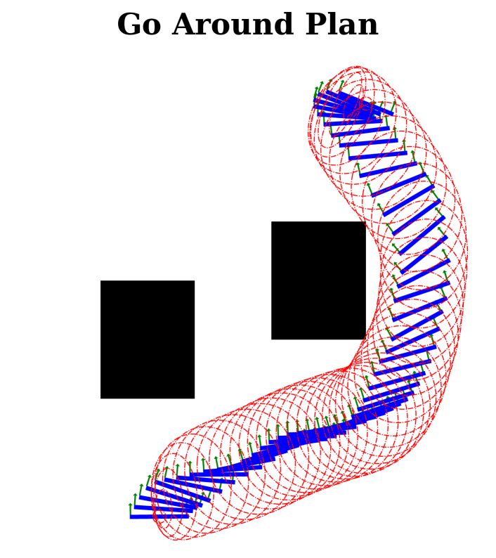
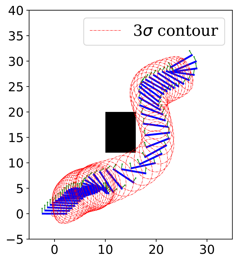
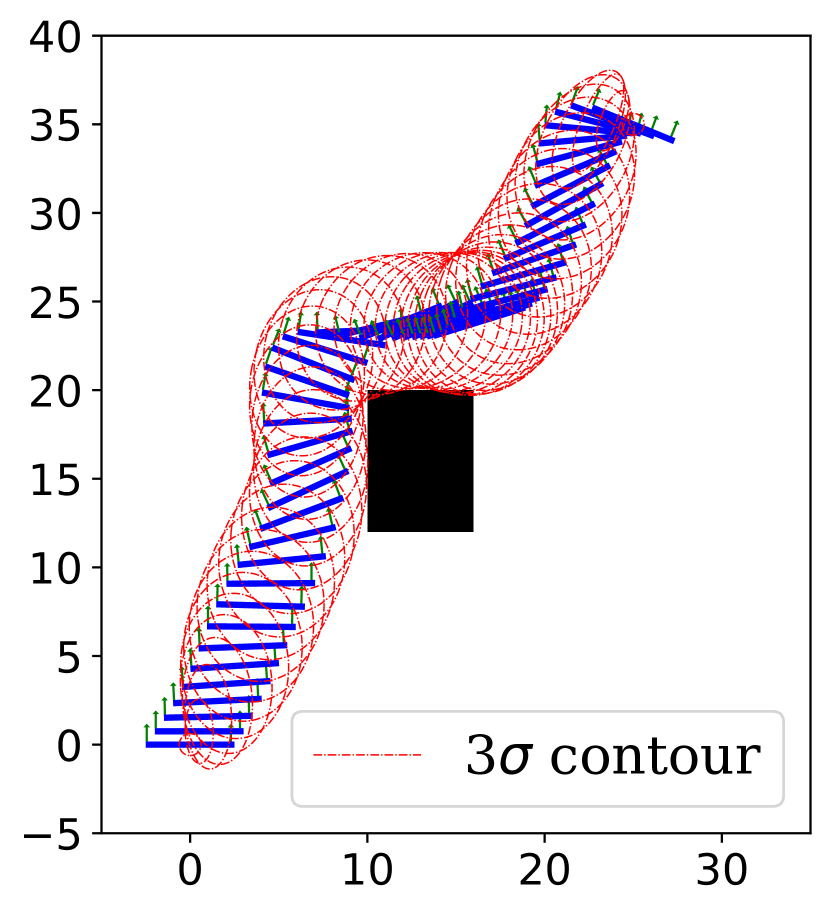
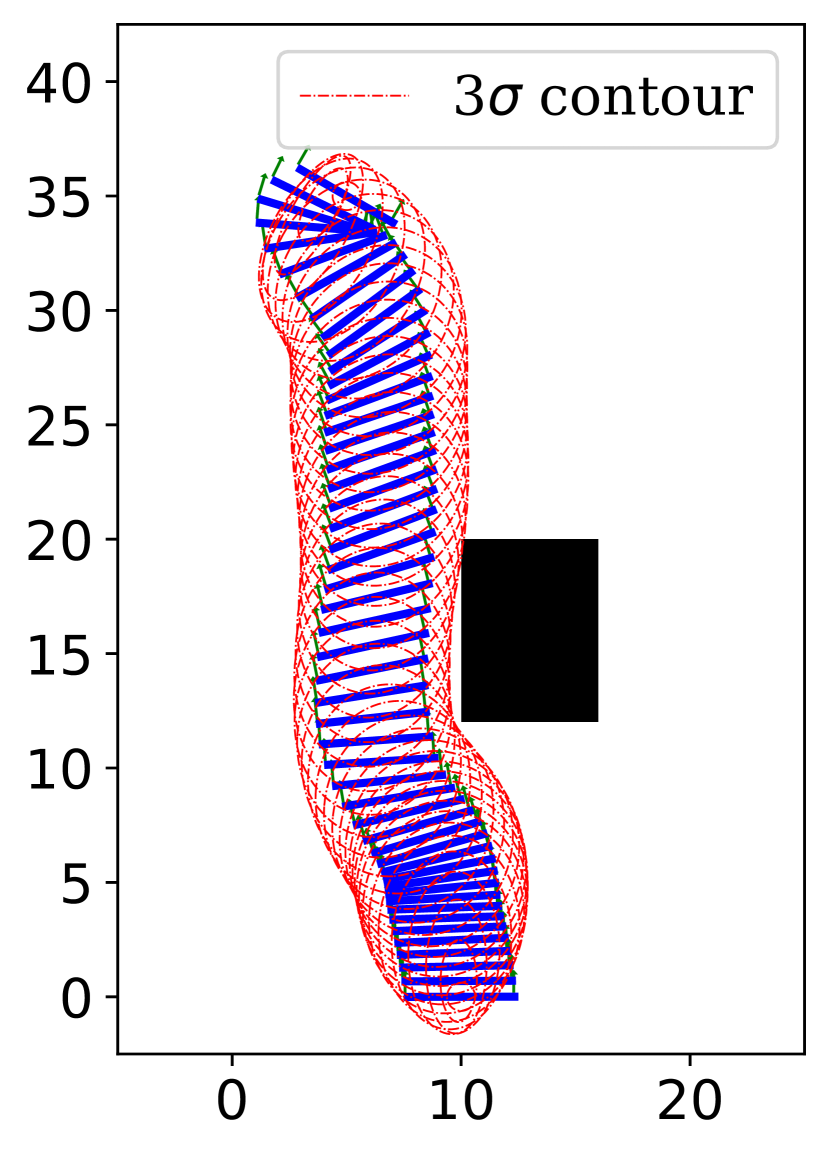
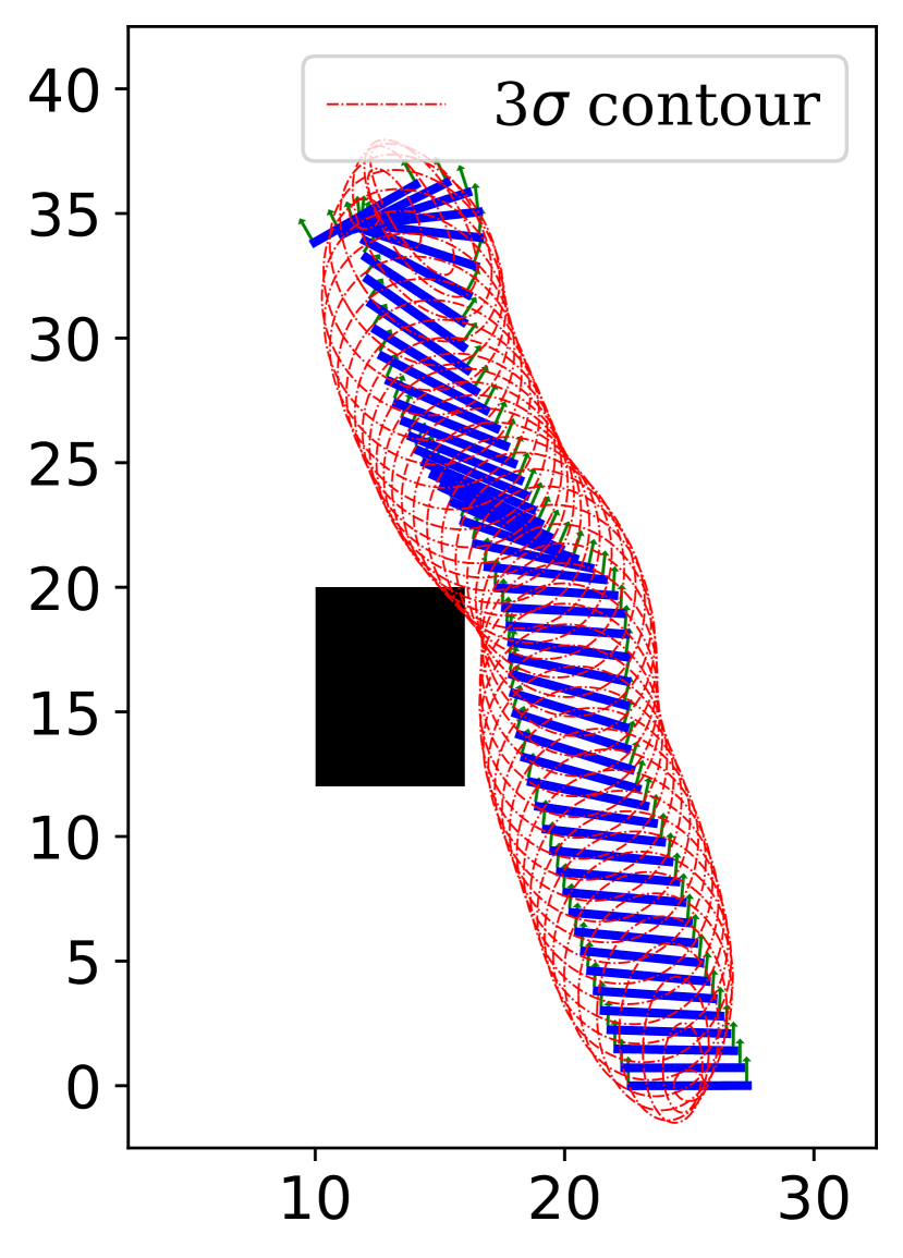
(b) Go through or go around a narrow gap? Robust motion planning through entropy regularization. As motion planning with obstacles is a naturally non-convex problem, the solution is multi-modal. In the decision-making for motion planning, the risk and robustness of the solution are taken into consideration in our formulation by introducing the entropy of into the objective. This section shows an experiment for the planar quadrotor to fly through a narrow gap [1]. Two motion plans are obtained for the same motion planning task, as shown in Fig. 2. One plan (go-through plan) is visually riskier than the other (go-around plan). Our formulation provides a computable metric to compare the total cost consisting of optimality and robustness, between the two plans. In Tab. I, we compute the sum of the prior and the collision costs, the entropy costs, and the total costs. By introducing lower entropy costs, our method selects the plan with lower risk over a shorter but riskier plan.
| Start | Goal | |
|---|---|---|
| Exp | ||
| Exp | ||
| Exp | ||
| Exp |
(c) More experiments with different settings. We did experiments for different settings. We have obstacle in the environment. The start and goal states in the experiments are specified in the following Tab. V.
VI conclusion
In this work, we propose a distributed Gaussian Variational Inference approach to solve motion planning under uncertainties. The optimal trajectory distribution to a stochastic control problem serves as the target posterior in a variational inference paradigm. We leveraged this inference’s underlying sparse factor graph structure and proposed a distributed computation framework to solve the VI problem in parallel on GPU. Numerical experiments show the effectiveness of the proposed methods on an LTV system, and comparison studies demonstrated the computational efficiency.
References
- [1] H. Yu and Y. Chen, “A gaussian variational inference approach to motion planning,” IEEE Robotics and Automation Letters, vol. 8, no. 5, pp. 2518–2525, 2023.
- [2] S. M. LaValle, Planning algorithms. Cambridge university press, 2006.
- [3] D. González, J. Pérez, V. Milanés, and F. Nashashibi, “A review of motion planning techniques for automated vehicles,” IEEE Transactions on intelligent transportation systems, vol. 17, no. 4, pp. 1135–1145, 2015.
- [4] N. Ratliff, M. Zucker, J. A. Bagnell, and S. Srinivasa, “Chomp: Gradient optimization techniques for efficient motion planning,” in IEEE international conference on robotics and automation, 2009, pp. 489–494.
- [5] J. Schulman, Y. Duan, J. Ho, A. Lee, I. Awwal, H. Bradlow, J. Pan, S. Patil, K. Goldberg, and P. Abbeel, “Motion planning with sequential convex optimization and convex collision checking,” The International Journal of Robotics Research, vol. 33, no. 9, pp. 1251–1270, 2014.
- [6] M. Kalakrishnan, S. Chitta, E. Theodorou, P. Pastor, and S. Schaal, “Stomp: Stochastic trajectory optimization for motion planning,” in IEEE international conference on robotics and automation, 2011, pp. 4569–4574.
- [7] K. J. Åström, Introduction to stochastic control theory. Courier Corporation, 2012.
- [8] S. Thrun, “Probabilistic robotics,” Communications of the ACM, vol. 45, no. 3, pp. 52–57, 2002.
- [9] S. Särkkä and A. Solin, Applied stochastic differential equations. Cambridge University Press, 2019, vol. 10.
- [10] M. Mukadam, X. Yan, and B. Boots, “Gaussian process motion planning,” in IEEE international conference on robotics and automation (ICRA), 2016, pp. 9–15.
- [11] M. Mukadam, J. Dong, X. Yan, F. Dellaert, and B. Boots, “Continuous-time gaussian process motion planning via probabilistic inference,” The International Journal of Robotics Research, vol. 37, no. 11, pp. 1319–1340, 2018.
- [12] M. D. Hoffman, D. M. Blei, C. Wang, and J. Paisley, “Stochastic variational inference,” Journal of Machine Learning Research, 2013.
- [13] D. M. Blei, A. Kucukelbir, and J. D. McAuliffe, “Variational inference: A review for statisticians,” Journal of the American Statistical Association, vol. 112, no. 518, pp. 859–877, 2017.
- [14] B. Ichter, J. Harrison, and M. Pavone, “Learning sampling distributions for robot motion planning,” in IEEE International Conference on Robotics and Automation (ICRA), 2018, pp. 7087–7094.
- [15] T. Osa, “Multimodal trajectory optimization for motion planning,” The International Journal of Robotics Research, vol. 39, no. 8, pp. 983–1001, 2020.
- [16] L. C. Cosier, R. Iordan, S. N. Zwane, G. Franzese, J. T. Wilson, M. Deisenroth, A. Terenin, and Y. Bekiroglu, “A unifying variational framework for gaussian process motion planning,” in International Conference on Artificial Intelligence and Statistics. PMLR, 2024, pp. 1315–1323.
- [17] T. Power and D. Berenson, “Constrained stein variational trajectory optimization,” IEEE Transactions on Robotics, 2024.
- [18] D. Hsu, L. E. Kavraki, J.-C. Latombe, R. Motwani, S. Sorkin et al., “On finding narrow passages with probabilistic roadmap planners,” in Robotics: the algorithmic perspective: 1998 workshop on the algorithmic foundations of robotics, 1998, pp. 141–154.
- [19] Y. Chen, T. T. Georgiou, and M. Pavon, “On the relation between optimal transport and schrödinger bridges: A stochastic control viewpoint,” Journal of Optimization Theory and Applications, vol. 169, pp. 671–691, 2016.
- [20] ——, “Optimal transport over a linear dynamical system,” IEEE Transactions on Automatic Control, vol. 62, no. 5, pp. 2137–2152, 2016.
- [21] H. Yu and Y. Chen, “Stochastic motion planning as gaussian variational inference: Theory and algorithms,” arXiv preprint arXiv:2308.14985, 2023.
- [22] T. D. Barfoot, C. H. Tong, and S. Särkkä, “Batch continuous-time trajectory estimation as exactly sparse gaussian process regression.” in Robotics: Science and Systems, vol. 10. Citeseer, 2014, pp. 1–10.
- [23] T. D. Barfoot, J. R. Forbes, and D. J. Yoon, “Exactly sparse gaussian variational inference with application to derivative-free batch nonlinear state estimation,” The International Journal of Robotics Research, vol. 39, no. 13, pp. 1473–1502, 2020.
- [24] H. J. Kappen, V. Gómez, and M. Opper, “Optimal control as a graphical model inference problem,” Machine learning, vol. 87, pp. 159–182, 2012.
- [25] M. Botvinick and M. Toussaint, “Planning as inference,” Trends in cognitive sciences, vol. 16, no. 10, pp. 485–488, 2012.
- [26] M. Toussaint, “Robot trajectory optimization using approximate inference,” in Proceedings of the 26th annual international conference on machine learning, 2009, pp. 1049–1056.
- [27] M. I. Jordan, Z. Ghahramani, T. S. Jaakkola, and L. K. Saul, “An introduction to variational methods for graphical models,” Machine learning, vol. 37, pp. 183–233, 1999.
- [28] I. V. Girsanov, “On transforming a certain class of stochastic processes by absolutely continuous substitution of measures,” Theory of Probability & Its Applications, vol. 5, no. 3, pp. 285–301, 1960.
- [29] M. Opper and C. Archambeau, “The variational Gaussian approximation revisited,” Neural Computation, vol. 21, no. 3, pp. 786–792, 2009.
- [30] O. Shental, P. H. Siegel, J. K. Wolf, D. Bickson, and D. Dolev, “Gaussian belief propagation solver for systems of linear equations,” in IEEE International Symposium on Information Theory, 2008, pp. 1863–1867.
- [31] J. Ortiz, T. Evans, and A. J. Davison, “A visual introduction to gaussian belief propagation,” arXiv preprint arXiv:2107.02308, 2021.
- [32] S. Anderson, T. D. Barfoot, C. H. Tong, and S. Särkkä, “Batch nonlinear continuous-time trajectory estimation as exactly sparse gaussian process regression,” Autonomous Robots, vol. 39, pp. 221–238, 2015.