Physical modelling of global macrosystems evolution

Abstract

The dynamics of growth and innovation often exhibit sudden, explosive surges, where systems remain quasi stable for extended periods before accelerating dramatically—often surpassing traditional exponential growth. This pattern is evident across various domains, including world population increases and rapid technological advancements. Although these phenomena share common characteristics, they are driven by different underlying mechanisms. In this paper, we introduce a unified framework to capture these phenomenologies through a theory of combinatorial innovation. Inspired by the Theory of the Adjacent Possible, we model growth and innovation as emerging from the recombination processes of existing elements of a system. By formalizing these qualitative ideas, we provide a mathematical structure that explains diverse phenomena, enables cross-system comparisons, and offers grounded predictions for future growth trajectories. Our approach distils the complexity of innovation into a more accessible yet robust framework, paving the way for a deeper and more flexible mathematical understanding of growth and innovation processes.

I Introduction

Many systems—ranging from biological Markov and Korotayev (2007); Grinin et al. (2015); Panov (2004) and social Von Foerster et al. (1960); Kapitza (1996); Korotayev (2013) to economic LePoire (2013); Korotayev (2005)—share a striking pattern of explosive growth and innovation. When we look at metrics like world population size Kremer (1993), average GDP per capita Korotayev (2009), or historical milestones Kurzweil (2004); LePoire (2015), the pace of increase over time is undeniable. These systems often grow at rates that surpass traditional exponential models Korotayev and LePoire (2020); Steffen et al. (2015), instead following hyperbolic functions Korotayev (2006); Panov (2005). This brings us to the concept of the ’singularity,’ where growth theoretically approaches infinity in a finite time. In real-world systems, this singularity can be interpreted as a harbinger of profound transformations or disruptive events on the horizon. While hyperbolic models fit the data impressively Korotayev (2009); Panov (2020), their true power and ability to explain real-world phenomena remain elusive. Additionally, the microscopic mechanisms driving such rapid growth are poorly understood, often leading to applying the same mathematical models to systems with very different behaviors.

The theory of ”singularity” is primarily phenomenological. Many innovation-driven systems have been effectively interpreted through combinatorial processes Koppl et al. (2018); Cortês et al. (2022a). In this framework, innovation and growth emerge from recombining elements within the system Kauffman (2000); Koppl et al. (2023), similar to assembling existing parts to create new tools. The Theory of the Adjacent Possible (TAP) Cortês et al. (2022b) proposes that systems can expand into their ”possible” space, which consists of elements that are not yet realized but are just one step away from being created  Kauffman (2000). Models based on this concept, such as the TAP equation, have been used to describe the growth of the world population Koppl et al. (2018) and GDP Koppl et al. (2023). Moreover, the concept of the Adjacent Possible has also been applied within the framework of Urn Models Tria et al. (2014); Di Bona et al. (2023), which reproduce key features of novelties dynamics, such as Zipf’s, Heaps’ and Taylor’s laws Tria et al. (2018); Loreto et al. (2016).

The combinatorial approach effectively replicates empirical data on a qualitative level Koppl et al. (2018); Steel et al. (2020) but often lacks a more quantitative and mathematical analysis. In this work, we aim to reconcile the hyperbolic growth observed in natural systems and the phenomenological theory of ”singularity” with the microscopically grounded theory of combinatorial innovation. This will allow us to distinguish between seemingly similar systems yet governed by different underlying processes. We demonstrate the versatility of our framework by applying it to a wide range of systems, including world population Korotayev (2006); Kapitza (1996), biological and cosmological phase shifts Kurzweil (2005); Korotayev (2020); Panov (2004), GDP per capita Korotayev (2005), and US patent records Youn et al. (2015).

We will end by discussing the concept of ”singularity”, which is often interpreted as a point where the extreme growth rate would lead to a qualitative change in the system’s behavior Kurzweil (2004); Panov et al. (2020); Korotaev (2006); Modis (2013); LePoire (2020). We argue that in real-world systems, which are discrete and finite, such a concept must be carefully considered, particularly when making predictions.

II The TAP equation: a paradigm for combinatorial growth

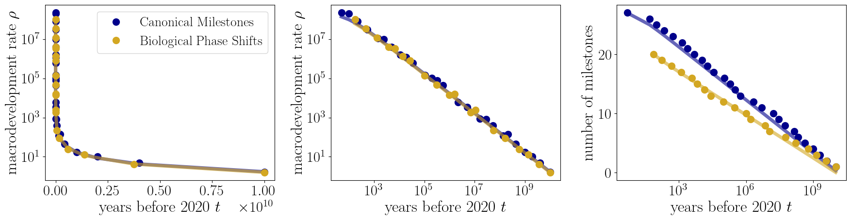
Figure 1: Evolution of Canonical Milestones and Biological Phase Transitions over time. Left. Macrodevelopment rate $\rho$ as a function of time, computed as the inverse of the inter-event time between successive milestones. The log-linear scale highlights the hyperbolic growth pattern, as exponential growth would appear as a straight line on this scale. Solid lines show the results of the fit discussed in Appendix C. Center. The same plot on a log-log scale, where the hyperbolic growth manifests as a straight line. The power-law exponent is $-1$, indicating a relationship of the form $y=1/x$. Right. Number of events as a function of time, plotted on a linear-log scale to emphasize the logarithmic behavior of milestone accumulation over time. The solid line represents equation 4, using the same parameters as those fitted to the macrodevelopment rate $\rho$.

The idea that innovations and growth arise as a combinatorial process is closely connected to the Theory of the Adjacent Possible (TAP) proposed by Kauffman et al. Kauffman (2000); Cortês et al. (2022b). The concept underlying the TAP is that the range of potential future developments is generated by the existing elements within the system, creating a space of possibilities where novel elements emerge from combinations of pre-existing ones. This framework applies to both physical entities (e.g., molecules, genes, tools) and conceptual ones (e.g., patents, songs, ideas).

This space of possibilities, known as the Adjacent Possible, contains all the unexplored elements that are just one step away from realization Kauffman (2000). Mathematically, this concept led to simple yet powerful models known as the TAP equation. If we denote by $M_{t}$ the number of elements in the system at time $t$, their evolution is governed by the number of combinations that can be formed from these elements:

$$M_{t+1}=(1-\mu)M_{t}+\sum_{i=1}^{M_{t}}\alpha_{i}\binom{M_{t}}{i}$$ (1)

Here, $\alpha_{i}$ represents coefficients that account for the realization probability of each combination, with typically decreasing values reflecting the increasing difficulty of forming longer combinations. For simplicity, we assume no extinction, setting $\mu=0$. We consider all terms in the summation starting from $i=1$, though some versions of the TAP equation start from $i=2$. These models are known for their explosive behavior, with growth rates exceeding exponential ones. TAP models have effectively described the growth of various systems, such as world population Koppl et al. (2018), GDP per capita, and the emergence of new technologies Koppl et al. (2023).

Analyzing equation 1 reveals that its analytic continuation diverges in finite time Cortês et al. (2022b). Hyperbolic functions naturally describe this behavior, featuring a singularity where the function diverges. However, it is important to recognize that this mathematical concept doesn’t apply to the real world, as no physical discrete system can exhibit infinite growth in finite time. Despite this limitation, hyperbolic functions have been widely used to interpret various systems, such as world population Korotayev (2006) and biological phase shifts in the field of biocosmology Korotayev (2020).

While the TAP equation offers a robust physical framework, its connection to hyperbolic functions has often been overlooked. The analytical continuation of the TAP equation naturally leads to hyperbolic expressions. For instance, in the simplest version of a TAP equation, with no extinction rate ($\mu=0$) and uniform coefficients ($\alpha_{i}=\alpha$ for any $i$), the model simplifies to:

$$M_{t+1}=M_{t}+\alpha\sum_{i=1}^{M_{t}}\binom{M_{t}}{i}$$

Using Pascal’s Triangle to evaluate the combinatorial term and considering the analytical continuation, we obtain:

$$\frac{dM_{t}}{dt}=\alpha(2^{M_{t}}-1)\approx\alpha 2^{M_{t}}$$

The solution to this differential equation is a hyperbolic function:

$$M_{t}=\log_{2}\left(\dfrac{1}{2^{-M_{0}}-\alpha(t-t_{0})}\right)$$ (2)

where $M_{0}$ is the initial number of elements in the system at time $t_{0}$. This is a hyperbolic expression featuring a singularity at time $t=t_{0}+\alpha^{-1}2^{-M_{0}}$. This result illustrates how hyperbolic trends observed in real-world data can arise from combinatorial models. In the following sections, we will demonstrate how different TAP models replicate various behaviors in real-world scenarios.

III MODELING GROWTH AND INNOVATION

In this section, we conduct a comprehensive analysis of various scenarios, applying the concepts discussed earlier. We examine five distinct datasets: the number of Canonical Milestones and Biological Phase Transitions (Section III.1), the growth of the world population and GDP (Section III.2), and technological innovations from US Patents (Section III.3). For each case, we select a specific combinatorial model represented by a particular form of the TAP Equation, solve them, and demonstrate that they align with the results found in previous research. Finally, we validate the model results using real-world data.

III.1 Biological Phase Transitions

In the realm of biocosmology, numerous studies have explored the emergence of paradigmatic events that have significantly influenced the history of the Universe and Life. These events include the origin of the Milky Way, the advent of life, the Cambrian explosion, the Hominoid revolution, and the emergence of democracy. Some studies refer to them as Canonical Milestones Kurzweil (2004, 2005); Modis (2003), while others as Biological Phase Transitions Panov (2004); Panov et al. (2020). Despite slight variations in data representation, both terms refer to the same phenomena with similar meanings and intentions. The two corresponding time series are presented in Appendix A.

When examining the time series for the occurrence of these milestones, authors from both perspectives have recognized a hyperbolic growth behavior (see Figure 1). Instead of analyzing the direct count of milestones, most researchers consider the ”inter time” Panov (2004); Korotayev (2020), which measures the time between two consecutive milestones. The inverse of the inter time, which represents the macrodevelopment rate $\rho_{t}$ and is effectively an approximation of the derivative of the milestone count $dM_{t}/dt$, closely follows a hyperbolic function with an exponent of $-1$:

$$CM\ :\ \rho_{t}=\frac{2.054}{t-2029},\quad PT\ :\ \rho_{t}=\frac{1.886}{t-2027}$$

for Canonical Milestones (CM) and Biological Phase Transitions (PT), respectively.

Starting with the general TAP equation 1 and assuming no extinction rate ($\mu=0$), our choice of the model relies on the selection of the parameter form for $\alpha$. Given that we know no specific mechanisms leading to the emergence of these phase transitions, we assume that any possible recombination of existing elements could be significant. To account for the increasing difficulty of combining a greater number of elements, we follow the idea presented in Cortês et al. (2022b) and set the coefficients to scale as a power law, $\alpha_{i}=\alpha^{i}$ for $\alpha\in(0,1)$. With this choice, the continuous TAP equation can be reformulated as Cortês et al. (2022b):

$$\frac{dM_{t}}{dt}=\sum_{i=1}^{M_{t}}\alpha^{i}\binom{M_{t}}{i}\approx(1+\alpha)^{M_{t}}=e^{\beta M_{t}}$$ (3)

with $\beta=\ln(1+\alpha)$. The solution to this equation leads to the following hyperbolic expression (details are reported in Appendix B):

$$M_{t}\approx\frac{1}{\beta}\log\left(\dfrac{1}{\beta(t-t_{0})+e^{-\beta M_{0}}}\right)$$ (4)

where $M_{0}$ is the initial condition of the system at time $t_{0}$. By deriving the number of the milestones $M_{t}$, we can compute the macrodevelopment rate $\rho_{t}$, which follows a hyperbolic function with an exponent of $-1$:

$$\rho_{t}=\frac{dM_{t}}{dt}\approx\dfrac{1}{\beta(t-t_{0})+e^{-\beta M_{0}}}$$ (5)

This model replicates the same analytical behavior observed in previous analyses Panov (2004); Kurzweil (2005). Importantly, these expressions emerge naturally from the combinatorial model’s structure, offering a straightforward physical interpretation rather than being derived solely from observed time series data. We can fit the time series using our model and compute the coefficient $\alpha$ that reproduces the actual number of milestones $M_{t}$. The results of this numerical analysis are presented in Figure 1 and in Appendix C.

The values of the coefficients in the two cases are $\alpha_{CM}=1.16\cdot 10^{-10}$ and $\alpha_{PT}=1.58\cdot 10^{-10}$. These model parameters represent the fraction of combinations occurring at any given time $t$, which indicates the rate of successful combinations that actually take place at each time step. We can refer to $\alpha$ as the macrodevelopment parameter of the system. The small difference in their values for Canonical Milestones and Biological Phase Transitions is due to the different events considered in the two time-series. However, the two parameters are comparable, reflecting a similar underlying process.

Additionally, the expressions we derived present a singularity at $t=t_{0}+\beta^{-1}e^{-\beta M_{0}}$, a time value at which the function theoretically diverges. However, the discrete version of the model in equation 3 does not exhibit any divergence in finite time, as it happens for real-world systems. We will explore the significance of this concept in Section IV.

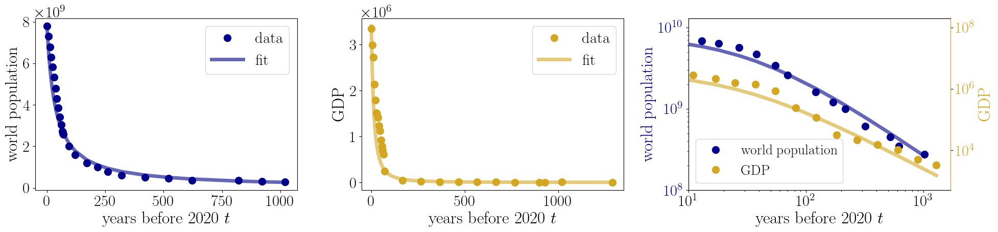
Figure 2: World population and GDP growth over time. Left. World population size from 1000 to 2020 CE. The sudden explosion in the last century suggests a rate that exceeds exponential growth. The solid line represents the hyperbolic fit, as discussed in Appendix C. Center. GDP aggregated for all countries, in millions of dollars, from 700 to 2018 CE. The hyperbolic growth pattern is again evident from the sharp rise in GDP in recent years. The solid line shows the hyperbolic fit, as detailed in Appendix C. Right World population and GDP evolution on a log-log scale. This scale highlights the hyperbolic growth, with a power law exponent of $1$ for world population and $2$ for GDP.

III.2 World Population and GDP

The growth of world population size over the years surpasses exponential rates, as widely recognized in prior literature Kremer (1993); Kapitza (1996). The seminal paper from 1960, ”Doomsday: Friday, 13 November, A.D. 2026” Von Foerster et al. (1960), was among the first to identify this phenomenon. The authors observed that demographic growth from the year 1 CE to 1958 CE followed a hyperbolic pattern:

$$N_{t}=\dfrac{C}{t^{*}-t}$$ (6)

with approximate constants $C\approx 2.15\cdot 10^{5}$ and $t^{*}\approx 2026$. The value $t^{*}$ represents the mathematical singularity of the hyperbolic curve, which was used to speculate about future population growth. This hyperbolic pattern has been verified from earlier periods Kremer (1993); Kapitza (1996) up to a million years ago and continues to be relevant for some years beyond 1958 Korotayev (2020).

Typically, these datasets are interpreted using dynamic models that consider the tradeoff between mortality and fecundity Lee (1980) without explicit accounting for individual interaction. In contrast, the combinatorial approach based on TAP has been employed to explain world population growth Koppl et al. (2018), although it does not focus on the specific types of interactions involved. Here, we show that by incorporating particular interaction terms into the combinatorial model, we can reproduce and predict the observed hyperbolic growth.

Starting with the general TAP equation 1, we select appropriate values for the parameters $\alpha_{i}$. Demographic growth is driven by reproductive processes, which can be modeled as pair interactions. We then hypothesize that the driving term is for $i=2$, corresponding to the number of pairs in the system:

$$\dfrac{dN_{t}}{dt}=\alpha^{2}\binom{N_{t}}{2}=\alpha^{2}\dfrac{N_{t}(N_{t}-1)}{2}\approx\gamma N_{t}^{2}$$ (7)

Given $N_{t}\gg 1$, we can neglect the linear term, focusing on the quadratic term and redefining $\gamma=\alpha^{2}/2$ as a birth rate. Notice that we do not consider direct mortality effects, so $\mu=0$ in equation 1.

The solution to equation 7 produces the hyperbolic curve (details are reported in Appendix B):

$$N_{t}\approx\dfrac{1}{N_{0}^{-1}-\gamma(t-t_{0})}$$ (8)

This result aligns with previous analyses Korotayev (2020). It is important to note that this solution is obtained using the continuous approximation of the model, while a discrete model would not exhibit any singularity. Results of the fit of the macrodevelopment parameter $\gamma$ are reported in Figure 2 and in Appendix C.

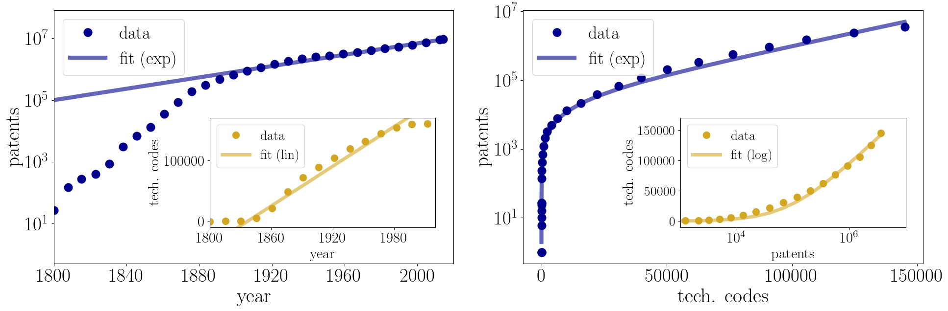
Figure 3: Evolution of the number of patents and technological codes over time. Left. Number of patents over time, shown on a log-linear scale. There is a rapid growth phase until approximately 1860, after which the trend becomes exponential. The solid line represents an exponential fit of the data starting from 1900. The inset shows the growth of the number of distinct technological codes in time on a linear scale. The solid line, following the empirical trend, highlights the linear growth of technological codes. Right. Number of patents as a function of technological codes, presented on a log-linear scale, which highlights the exponential growth of patents. As discussed in Appendix C, the solid line represents the fit. The inset shows the number of technological codes versus the number of patents. In this case, the trend is reversed. The linear-log scale highlights the logarithmic growth of technological codes. The solid line represents the model fit.

Furthermore, some works Korotayev and LePoire (2020); Korotayev (2020) mistakenly equate the hyperbolic patterns of demographic growth with those of Canonical Milestones, suggesting they are generated by the same process. However, these situations are distinct, as demonstrated by the different models used to fit the data. For Canonical Milestones ($M_{t}$), the hyperbolic pattern pertains to the rate, described by the equation 5, which involves all combinatorial terms. In contrast, for the world population, the hyperbolic pattern emerges directly in $N_{t}$ (Eq. 8), where only pair interactions are considered.

Finally, we extend our analysis to GDP per capita, reaffirming previous findings within the new combinatorial framework. Many researchers have postulated a relationship between GDP growth and world population Malthus (2023); Acemoglu (2008). According to Malthusian macroeconomic principles, the GDP $K_{t}$ grows at a rate proportional to the size of the population $N_{t}$. We can represent this growth rate with a combinatorial term proportional to $K_{t}N_{t}$ Korotayev (2009). Additionally, empirical data show that GDP’s behavior over the years closely mirrors the square of the population $N_{t}\approx\sqrt{K_{t}}$ Korotayev (2005). Using these observations, the GDP growth rate can be expressed as:

$$\dfrac{dK_{t}}{dt}=\delta K_{t}N_{t}\approx\delta K_{t}^{3/2}$$ (9)

where $\delta$ is the macrodevelopment parameter. The solution is a hyperbolic curve with an exponent of 2 (analytical details are given in Appendix B):

$$K_{t}\approx\dfrac{1}{\left(K_{0}^{-1/2}-\delta t\right)^{2}}$$ (10)

This result matches the expression fitted to the data in previous works Korotayev (2009). Once again, this hyperbolic behavior is explained within the combinatorial growth framework. Results of the fit of the parameter $\delta$ are reported in Figure 2 and Appendix C.

III.3 Technological Innovations: the Case of US Patents

Technological innovations, as demonstrated through patenting activities, provide an effective example of combinatorial growth. Patents are characterized by a set of codes, which reveal the underlying technological capabilities used in the invention. As a result, patents naturally emerge as combinations of technological codes. However, this system differs significantly from those previously explored, as the number of patents displays an exponential, rather than hyperbolic, increase over time Youn et al. (2015).

Due to this exponential behavior, previous frameworks have either omitted the example of US patents or approached it differently. In some instances, the TAP equation was employed to explain the distribution of descendants of any given patent, with minimal consideration for their temporal evolution Koppl et al. (2023). In another study Youn et al. (2015), the authors conducted a detailed statistical analysis of the US patents dataset, focusing on the combinatorial processes underlying the creation of new technologies. However, no model was proposed to reproduce the observed dynamics.

It is easy to show that our framework can also describe the dynamics of patents and reproduce the essential features of the data. The left panel of Figure 3 illustrates the exponential growth of the number of patents over time when plotted on a log-linear scale. Conversely, the behavior of technological codes is linear rather than exponential, as shown in the inset. As shown in the right panel of Figure 3, plotting the number of patents relative to the number of distinct technological codes reveals an exponential relationship.

To build the model, we exploit the idea that patents are created through the combination of technological codes. Patents can theoretically involve any number of codes, with larger combinations presenting more challenges to be realized. Therefore, we consider all terms within equation 1 to establish an exponential model, similar to the approach outlined in Section III.1:

$$\frac{dP_{C}}{dC}=\sum_{i=1}^{C}\alpha^{i}\binom{C}{i}\approx e^{\beta C}$$ (11)

with $\beta=\ln(1+\alpha)$, where $\alpha$ is the usual macrodevelopment rate of the system. Here, $C$ represents the number of technological codes, while $P_{C}$ denotes the number of patents associated with a given code $C$. In this model, we treat the number of technological codes as the timescale, $C$. Consequently, the solution of equation 11 is:

$$P_{C}\propto\dfrac{1}{\beta}e^{\beta C},\quad C_{P}\propto\dfrac{1}{\beta}\log\beta P$$ (12)

This equation replicates the observed trends of patents and technological codes, as shown in the right panel of Figure 3. We also present the specific curve obtained by fitting the data. Further details regarding the coefficients used in this model are provided in Appendix C.

Moreover, the relationships outlined in equation 12 enable us to recover the temporal growth of these two quantities, as shown in the left panel of Figure 3. In regions where $C(t)$ approximates linearity, an exponential growth pattern emerges for patents, such that $P(t)\propto e^{t}$. It is important to stress that, in this case, the model does not produce any singularity, even if the underlying mechanism is analogous to that applied to other systems. This showcases the versatility of the TAP equation and the theory of combinatorial innovation to describe a wide variety of different systems with similar but yet different underlying dynamics.

IV Discussion

The mathematical singularity arising from the hyperbolic behaviors described in Section III has been subject to various interpretations. The concept of “Singularity” was already mentioned in the work of Von Foerster et al. Von Foerster et al. (1960), who provocatively identified a specific date for the so-called ”Doomsday,” projected to occur on 13 November 2026. More recently, scholars offered two main interpretations of this concept. The first, as suggested by Von Foerster et al. (1960), argues that such a singularity indicates that rapid growth is unsustainable in real finite systems. This view implies that a slowdown in growth must occur before any potential explosive scenario Korotayev (2020); Korotayev and LePoire (2020); Modis (2013). In this interpretation, the mathematical divergence can be seen as a potential indicator of this deceleration getting closer. Indeed, in many systems, it is reasonable to expect a deceleration due to the presence of limiting factors such as the finite availability of resources. Nonetheless, our mathematical analysis reveals that inferring this slowdown from the data may be very tricky. First, the discrete versions of the models, which represent the actual dynamics of real-world systems, do not exhibit any singularity. The discrete models can be indeed used to forecast growth beyond this theoretical limit, as detailed in Appendix C. Secondly, our models do not explicitly account for external limiting factors, which are the true drivers of any changes in the system. As a result, these simple models are not able to predict any shift in the system’s evolution. This makes the singularity value practically unrelated to any constraints or deceleration.

Conversely, some authors, particularly in the Big History field, view the singularity as an indicator of upcoming transitions or technological shifts Kurzweil (2005); Panov (2020); Nazaretyan (2015). For instance, the concept of Threshold 9 in the field of Big History Nazaretyan (2016) suggests that humanity is approaching a profound global paradigm shift (the threshold) that will significantly impact both technology and evolution Kurzweil (2005). Some authors even speculate about post-singularity civilizations Panov (2011). This second interpretation often relies on extrapolations from data without direct evidence that current growth rates will continue indefinitely, positioning such analyses more within the realm of philosophical speculation, though they inspire fascinating and stimulating discussions. From a technical perspective, attempts to extrapolate precise years from the data can lead to peculiar results. For example, in Von Foerster et al. (1960), the authors calculated the value $N_{t}=1$ from the world population curve and interpreted it as ”Adam’s birth,” resulting in a date nearly 200 billion years in the past. Similarly, some predictions appear strikingly accurate but are essentially coincidental, such as the singularity in GDP per capita growth estimated for 2005 Korotayev (2009), which is closely aligned with the 2008 financial crisis.

Finally, it is important to stress that estimating a reliable singularity value is almost impossible due to the high value of statistical error. As noted in Von Foerster et al. (1960), the year obtained from fitting data can vary substantially depending on the choice of the last observation. For instance, if Charlemagne, with data until 800 CE, had predicted a singularity, he would have projected it 300 years into the future, while Napoleon, using more recent data, would have predicted it just 30 years ahead. In the very same way, our estimates of singularities, presented in Appendix C, differ from previous analyses in the literature due to the updated data. In certain cases, large time intervals considered in the analysis result in wide confidence bounds for the numerical value of the singularity, making it even more difficult to obtain a reliable estimate.

V Conclusions

This study investigates the dynamics of growth and innovation, offering a unified approach for modeling and understanding it. Innovation dynamics often exhibit hyperbolic trends, which have been studied and interpreted in various ways in the literature. However, a coherent framework that models these processes from a physical and mathematical perspective has been lacking. By leveraging a combinatorial approach based on the Theory of Adjacent Possible (TAP), we provide a comprehensive theoretical foundation to interpret these phenomena. We investigated several distinct scenarios, demonstrating how our framework can successfully replicate the main characteristics of growth trends. We analyzed four key cases: biological milestones (Canonical Milestones and Biological Phase Transitions), world population, GDP growth, and technological innovations as seen through U.S. patent data. In each case, the models allow us to estimate the macrodevelopment parameter from the data, enabling us to quantify the system’s growth rate.

This paper demonstrates how a combinatorial framework can offer a coherent interpretation of growth and innovation processes across diverse domains. Future research should explore applying these models to other complex systems, such as biological or evolutionary processes, where similar growth dynamics are observed. The main limitation of our approach is that it does not consider any external factor acting on the system, which is relevant in most cases. Given the simplicity and interpretability of our approach, future work could focus on incorporating external constraints, such as resource limitations, to produce more accurate descriptions and forecasts of system behavior. Another promising direction is investigating the connection between this framework and the triggering mechanisms described in other discovery processes Tria et al. (2014); Di Bona et al. (2023); Bellina et al. (2024). In this view, the emergence of innovations is explained through exploring a network, where each novelty opens up the possibility for further developments. Establishing a connection between these frameworks could further advance our understanding of innovation processes and achieve a comprehensive theory of innovation.

Appendix A Data sources

Canonical Milestones

Modis-Kurzweil time series Modis (2003); Kurzweil (2005) considers key evolutionary and technological milestones, focusing on the interplay between demographic growth and technological innovation. They are also referred to as Canonical Milestones. Starting from the Big Bang, it outlines 27 major critical events in the history of the universe, from the formation of galaxies to the rise of the Internet. The time in parentheses refers to the number of years before 2020.

1. Origin of Milky Way and First Stars (10 billion years): The formation of the Milky Way galaxy and the first stars.

2. Origin of Life on Earth, Formation of the Solar System (4 billion years ago): The emergence of life on Earth and the formation of the solar system and Earth’s oldest rocks.

3. First Eukaryotes and Invention of Sex (2 billion years): The development of eukaryotic cells, the emergence of sexual reproduction, atmospheric oxygen, photosynthesis, and plate tectonics.

4. First Multicellular Life (1 billion years): The appearance of multicellular organisms such as sponges, seaweeds, and protozoans.

5. Cambrian Explosion and First Vertebrates (430 million years): A period of rapid diversification of life, with the emergence of invertebrates, vertebrates, plants, and amphibians.

6. First Mammals and Dinosaurs (210 million years): The rise of mammals, birds, and dinosaurs.

7. First Flowering Plants (139 million years): The appearance of angiosperms, or flowering plants.

8. Mass Extinction and First Primates (54.6 million years): An asteroid impact causes mass extinction, including the dinosaurs, and the emergence of primates.

9. First Hominids (28.5 million years): The appearance of early human ancestors.

10. First Orangutans and Proconsul (16.5 million years): The origin of orangutans and the early ape genus Proconsul.

11. Chimpanzees and Humans Diverge (5.1 million years): The evolutionary split between humans and chimpanzees, with the earliest evidence of bipedalism in hominids.

12. First Stone Tools and Homo Erectus (2.2 million years): The development of early stone tools and the appearance of Homo erectus.

13. Emergence of Homo Sapiens (555,000 years ago): The first appearance of anatomically modern humans.

14. Domestication of Fire (325,000 years): Homo heidelbergensis begins controlling fire for cooking and warmth.

15. Human DNA Differentiation (200,000 years): The divergence of different human DNA types.

16. Emergence of Modern Humans (105,700 years): The earliest evidence of modern humans and their burial practices.

17. Rock Art and Protowriting (35,800 years): The creation of early forms of symbolic communication through rock art.

18. Techniques for Starting Fire (19,200 years): The development of techniques for creating fire independently.

19. Invention of Agriculture (11,000 years): The shift from hunter-gatherer societies to settled farming communities.

20. Invention of the Wheel and Writing (4907 years): The development of the wheel, writing systems, and the rise of early civilizations in Egypt and Mesopotamia.

21. Democracy and the Axial Age (2437 years): The rise of city-states, democracy in Greece, and the teachings of figures like Buddha.

22. Invention of Zero and Fall of Rome (1440 years): The development of the concept of zero and the fall of the Roman Empire.

23. Renaissance and the Scientific Method (539 years): A period of cultural rebirth in Europe, marked by the discovery of the New World and the development of the scientific method.

24. Industrial Revolution (225 years): The advent of steam engines, political revolutions, and the rise of industrial economies.

25. Modern Physics and Technological Advances (100 years): Major breakthroughs in physics, radio, electricity, automobiles, and aviation.

26. Nuclear Energy and the Cold War (50 years): The discovery of DNA’s structure, the invention of the transistor, and the onset of the Cold War.

27. Internet and Human Genome Sequencing (5 years): The sequencing of the human genome and the rise of the internet as a transformative technology.

Biological Phase Transitions

Panov time series Panov (2020); Korotayev and LePoire (2020) represents a historical trajectory of complexity growth, marking key transitions in the development of life and civilization on Earth. They are also referred to as Biological Phase Transitions. This series of 20 events covers critical points in universal and human history, from the origin of life to modern history. Each event signifies a substantial increase in complexity, accelerating over time as each phase becomes shorter. The time in parentheses refers to the number of years before 2020.

1. Origin of Life (4 billion years): The emergence of life, with the biosphere dominated by nucleus-less prokaryotes for the first 2-2.5 billion years.

2. Neoproterozoic Revolution (1.5 billion years): Cyanobacteria enrich the atmosphere with oxygen, leading to the extinction of many anaerobic prokaryotes and the rise of aerobic eukaryotes and multicellular life.

3. Cambrian Explosion (590-510 million years): A rapid diversification of life forms, leading to the emergence of all modern animal phyla, including vertebrates.

4. Reptiles Revolution (235 million years): A mass extinction wipes out most Paleozoic amphibians, allowing reptiles to dominate terrestrial life.

5. Mammalian Revolution (66 million years): The extinction of the dinosaurs marks the beginning of the dominance of mammals on land.

6. Hominoid Revolution (25-20 million years): A significant evolutionary event that leads to the rise of numerous Hominoidae genera, many more than exist today.

7. Quaternary Period (4.4 million years): The first primitive members of the Homo genus diverge from other Hominoidae.

8. Palaeolithic Revolution (2.0-1.6 million years): The emergence of Homo habilis and the first use of stone tools.

9. Chelles Period (700,000-600,000 years): The discovery of fire and the rise of Homo erectus.

10. Acheulean Period (400,000 years): The standardization of symmetric stone tools.

11. Neanderthal Culture Revolution (150,000-100,000): Homo sapiens neanderthalensis appears with fine stone tools and burial practices, suggesting the beginnings of primitive religion.

12. Upper Palaeolithic Revolution (40,000 years): Homo sapiens sapiens becomes the dominant species, developing advanced hunting tools and imitative art.

13. Neolithic Revolution (12,000-9,000 years): The shift from foraging to food production, marking the rise of agriculture.

14. Urban Revolution (6000-5000 years): The emergence of state formations, written language, and the first legal codes.

15. Imperial Antiquity and Iron Age (2800-2500 years): The rise of empires and the Axial Age, marked by cultural revolutions and thinkers like Zarathustra, Socrates, and Buddha.

16. Beginning of the Middle Ages (1600-1400 years): The fall of the Western Roman Empire, the spread of Christianity and Islam, and the dominance of feudal economies.

17. Modern Period and First Industrial Revolution (570-470 years): The rise of manufacturing, the printing press, and the cultural revolutions of the early modern era.

18. Second Industrial Revolution (190-180 years): The mechanization of industry, with the rise of steam power, electricity, and early globalization through the telegraph.

19. Information Revolution (70 years): The transition to post-industrial society, where the majority of workers in industrialized countries are employed in information-related fields or services.

20. Crisis and Collapse of the Communist Block (30 years): Information globalization accelerates following the political and economic changes marked by the end of the Cold War.

World Population

The data on world population growth was retrieved from Gapminder (https://www.gapminder.org/). As the platform states, ”Gapminder combines data from multiple sources into unique coherent time series that can’t be found elsewhere.” The time series provides estimates of world population size from $10,000$ BCE to the present day. For this analysis, we considered the period from $1000$ to $2020$ CE.

GDP

The data on GDP growth was obtained from the Maddison Project Database 2020 Bolt and Van Zanden (2020). According to the website, ”The Maddison Project Database provides information on comparative economic growth and income levels over the very long run. The 2020 version of this database covers 169 countries and the period up to 2018”. We aggregated the time series of all $169$ countries to create a global GDP time series, considering data from $700$ CE to $2018$ CE.

US Patents

The data on U.S. patents was retrieved from the United States Patent and Trademark Office (USPTO) (http://www.uspto.gov/patents/) Lyons (2003). This source provides time series data on all U.S. patents from $1800$ CE to $2020$ CE. Patents are classified by technological codes according to the U.S. Patent Classification System, where each code is represented by an alphanumeric string. From this data, we constructed a time series for both the number of patents and the associated technological codes over time.

Appendix B General Solution of Hyperbolic Differential Equation

In this appendix, we explicitly solve the differential equation governing the models presented in Section III.

First, consider the differential equation of the form displayed in Section III.1, given by

$$\dfrac{dx}{dt}=e^{ax},$$

which can be solved by the separation of variables:

$$e^{-ax}dx=dt.$$

Integrating $dx$ from $x_{0}$ to $x_{t}$, and $dt$ from $t_{0}$ to $t$, we obtain:

$$-\dfrac{e^{-ax_{t}}}{a}+\dfrac{e^{-ax_{0}}}{a}=t-t_{0}.$$

Inverting this relation, we get the explicit form of the solution:

$$x_{t}=\dfrac{1}{a}\log\left(\dfrac{1}{a(t-t_{0})+e^{-aM_{0}}}\right).$$

This expression presents a mathematical singularity at the point $t=t_{0}+a^{-1}e^{-ax_{0}}$.

For a differential equation of the form displayed in Section III.2:

$$\dfrac{dx}{dt}=ax^{b},$$

we solve by separation of variables:

$$x^{-b}dx=adt.$$

Integrating $dx$ from $x_{0}$ to $x_{t}$, and $dt$ from $t_{0}$ to $t$, we obtain:

$$\dfrac{x^{1-b}}{1-b}-\dfrac{x_{0}^{1-b}}{1-b}=a(t-t_{0}).$$

Inverting this relation, we obtain the explicit form of the solution:

$$x_{t}=\left[(1-b)\left(a(t-t_{0})-\frac{x_{0}^{1-b}}{b-1}\right)\right]^{\frac{1}{1-b}}.$$

When $b>1$, this expression presents a divergence at the point $t^{*}=t_{0}+a^{-1}(b-1)^{-1}x_{0}^{1-b}$.

Finally, the differential equation reported in Section III.3 presents simple exponential growth:

$$\dfrac{dP}{dC}=e^{aC}.$$

Integrating both sides, we get

$$P_{C}=\dfrac{e^{aC}}{a}-\dfrac{e^{aC_{0}}}{a}+P_{0}.$$

This expression shows no divergence in finite time, meaning there is no singularity.

Appendix C Results of numerical analysis

In this section, we present the results of fitting the models to real data and discuss the meaning of the parameters used. For all analyses, the time variable $t$ is defined as the time before 2020, with the year 2020 corresponding to $t=0$.

For both Biological Phase Transitions and Canonical Milestones, the macrodevelopment rate $\rho_{t}=\frac{dM_{t}}{dt}$ follows the expression (Eq. 5):

$$\rho_{t}=\dfrac{1}{e^{-\beta M_{0}}-\beta(t-t_{0})}.$$

We fitted $1/\rho_{t}$ against $t$ using a linear model, setting $t_{0}=5$ for Canonical Milestones and $t_{0}=30$ for Biological Phase Transitions. The initial values of $M_{0}$ were taken as $27$ and $20$, respectively. We fitted the parameter $\beta$ and then calculated the macrodevelopment rate $\alpha$ using the relation $\beta=\ln(1+\alpha)$:

$$\begin{cases}\beta_{CM}=(0.773\pm 0.009)\times 10^{-10}\\ \alpha_{CM}=(1.16\pm 0.02)\times 10^{-10}\end{cases}$$

$$\begin{cases}\beta_{BT}=(0.949\pm 0.010)\times 10^{-10}\\ \alpha_{BT}=(1.58\pm 0.03)\times 10^{-10}\end{cases}$$

The singularity time $t^{*}$ can be calculated as:

$$t^{*}=t_{0}-\frac{1}{\beta}e^{-\beta M_{0}},$$

which gives:

$$t^{*}_{CM}=-7.1\pm 2.7\ (2027.1)$$

$$t^{*}_{BT}=16.0\pm 11.2\ (2004.0)$$

In the case of Biological Phase Transitions, the singularity appears in the past because the time series ends $30$ years before 2020. This highlights the ambiguity and arbitrariness in estimating the exact singularity time, which strongly depends on the chosen endpoint of the dataset. Our results also differ from those reported in Korotayev and LePoire (2020), probably due to different fitting techniques. Additionally, the quite large error margins prevent a precise estimate of the singularity year.

The macrodevelopment parameter $\alpha$ represents the combinatorial success rate, quantifying the fraction of potential combinations that actually produce successful innovations. The two parameters $\alpha_{CM}$ and $\alpha_{BT}$ are close in magnitude, reflecting the same underlying process, irrespective of the specific events considered in the two time series. From the parameters, we can estimate the number of expected new Canonical Milestones in the future. From the discrete version of the model:

$$M_{t+1}-M_{t}=\sum_{i=1}^{M_{t}}\alpha^{i}\binom{M_{t}}{i},$$

we can compute the discrete macrodevelopment rate $\rho_{t}=M_{t+1}-M_{t}$. For $M_{t}=27$, this is approximately $\rho_{t}\approx 0.10$. This implies that the next Canonical Milestone is expected to occur about $1/\rho_{t}=10$ years after $t_{0}=2015$, around the year 2025.

After this point, with $M_{t}=28$, the rate increases to $\rho_{t}\approx 0.20$, meaning the next milestone is expected in the next $5$ years, thus around 2030. Notably, this prediction bypasses the singularity at 2027, emphasizing that in the discrete version of the model, the concept of a singularity does not apply. The discrete formulation thus allows for more accurate forecasting of future events, overcoming the limitations of continuous models.

In the case of the world population, we follow the same procedure. Starting from the equation:

$$N_{t}=\dfrac{1}{N_{0}^{-1}-\gamma(t-t_{0})},$$

and fitting $1/N_{t}$ against time, imposing $t_{0}=0$ and $N_{0}\approx 7.79\cdot 10^{8}$, we obtain:

$$\gamma=(1.61\pm 0.06)\times 10^{-12},$$

$$t^{*}_{WP}=\dfrac{1}{N_{0}\gamma}=-34.6\pm 0.6\ (2054.6).$$

Note the relatively small error in the singularity estimate, which is due to the shorter time interval considered for this dataset compared to the previous ones, reducing uncertainty. Once again, our predictions differ from previous literature due to the use of different data and time periods.

The macrodevelopment parameter $\gamma$ can be interpreted as a birth rate, indicating the fraction of potential interactions between individuals that lead to successful reproduction. Considering the discrete version of the model:

$$N_{t+1}-N_{t}\approx\gamma N_{t}^{2},$$

we find, for example, that with the current population size of approximately $8\cdot 10^{9}$, the predicted increase in the next year is about $\gamma N_{t}^{2}\approx 1\cdot 10^{8}$. This estimate aligns well with the actual population growth observed between 2020 and 2023, which averaged around $0.75\cdot 10^{8}$ per year.

For GDP growth, we use the equation:

$$K_{t}\approx\dfrac{1}{\left(K_{0}^{-1/2}-\delta(t-t_{0})\right)^{2}}.$$

By fitting the linear relation between $1/K_{t}^{2}$ and time, and using the initial conditions $t_{0}=0$ and $K_{0}=3.402405\cdot 10^{6}$, we obtain:

$$\delta=(1.96\pm 0.03)\times 10^{-5},$$

$$t^{*}_{GDP}=\dfrac{1}{\sqrt{K_{0}}\delta}=-26.7\pm 0.4\ (2046.7).$$

The macrodevelopment parameter $\delta$ represents the rate of GDP growth. Using the discrete dynamics:

$$K_{t+1}-K_{t}\approx\delta K_{t}^{3/2},$$

we estimate that in the year following 2020, GDP should grow by approximately $\delta K_{t}^{3/2}\approx 1.2\cdot 10^{5}$, consistent with the growth rate measured in the last three years (2020-2023), which was about $3\%$ per year.

Finally, the number of patents as a function of the number of technological codes is given by:

$$P_{C}=\dfrac{e^{\beta C}}{\beta}-\dfrac{e^{\beta C_{0}}}{\beta}+P_{0}.$$

From the exponential fit, and setting $C_{0}$ and $P_{0}$, we find $\beta=(4.18\pm 0.02)\times 10^{-5}$. In this case, there is no singularity, even in the continuous version of the model.

The macrodevelopment parameter $\alpha=e^{\beta}-1$ reflects the growth rate of the number of patents relative to the number of available technological codes. The discrete dynamics can be expressed as:

$$P_{C+1}-P_{C}=\sum_{i=1}^{C}\alpha^{i}\binom{C}{i}.$$

By substituting the actual number of technological codes $C=160586$ in the year 2020, we can compute the expected number of patents introduced when $C$ increases by one, i.e., when a new technological code is created. This results in approximately $P_{C+1}-P_{C}\approx 821$ new patents. In other words, at this stage of the system’s evolution, it takes roughly $821$ patents to introduce a single new technological code.

References

- Markov and Korotayev (2007) A. V. Markov and A. V. Korotayev, Palaeoworld 16, 311 (2007).
- Grinin et al. (2015) L. Grinin, A. V. Korotayev, and A. V. Markov, (2015).
- Panov (2004) A. Panov, Byulleten’Nauchnokul’turnogo tsentra SETI Akademii kosmonavtiki im. KE Tsiolkovskogo 7, 4 (2004).
- Von Foerster et al. (1960) H. Von Foerster, P. M. Mora, and L. W. Amiot, Science 132, 1291 (1960).
- Kapitza (1996) S. P. Kapitza, Physics-uspekhi 39, 57 (1996).
- Korotayev (2013) A. Korotayev, Evolution: Development within Big History, Evolutionary and World-System Paradigms , 69 (2013).
- LePoire (2013) D. LePoire, Evolution 3, 108 (2013).
- Korotayev (2005) A. Korotayev, Journal of World-Systems Research , 79 (2005).
- Kremer (1993) M. Kremer, The quarterly journal of economics 108, 681 (1993).
- Korotayev (2009) A. Korotayev, Systemic development: Local solutions in a global environment , 103 (2009).
- Kurzweil (2004) R. Kurzweil, The law of accelerating returns (Springer, 2004).
- LePoire (2015) D. LePoire, Emergence: Complexity and organization 17, 1E (2015).
- Korotayev and LePoire (2020) A. V. Korotayev and D. J. LePoire, The 21st Century Singularity and Global Futures (Springer, 2020).
- Steffen et al. (2015) W. Steffen, W. Broadgate, L. Deutsch, O. Gaffney, and C. Ludwig, The Anthropocene Review 2, 81 (2015).
- Korotayev (2006) A. Korotayev, History & mathematics: Historical dynamics and development of complex societies , 44 (2006).
- Panov (2005) A. D. Panov, Advances in Space Research 36, 220 (2005).
- Panov (2020) A. Panov, The 21st Century Singularity and Global Futures: A Big History Perspective , 439 (2020).
- Koppl et al. (2018) R. Koppl, A. Devereaux, J. Herriot, and S. Kauffman, arXiv preprint arXiv:1811.04502 (2018).
- Cortês et al. (2022a) M. Cortês, S. A. Kauffman, A. R. Liddle, and L. Smolin, arXiv preprint arXiv:2204.09378 (2022a).
- Kauffman (2000) S. A. Kauffman, Investigations (Oxford University Press, 2000).
- Koppl et al. (2023) R. Koppl, R. C. Gatti, A. Devereaux, B. D. Fath, J. Herriott, W. Hordijk, S. Kauffman, R. E. Ulanowicz, and S. Valverde, Explaining technology (Cambridge University Press, 2023).
- Cortês et al. (2022b) M. Cortês, S. A. Kauffman, A. R. Liddle, and L. Smolin, arXiv preprint arXiv:2204.14115 (2022b).
- Tria et al. (2014) F. Tria, V. Loreto, V. D. P. Servedio, and S. H. Strogatz, Scientific reports 4, 5890 (2014).
- Di Bona et al. (2023) G. Di Bona, A. Bellina, G. De Marzo, A. Petralia, I. Iacopini, and V. Latora, arXiv preprint arXiv:2307.06147 (2023).
- Tria et al. (2018) F. Tria, V. Loreto, and V. D. Servedio, Entropy 20, 752 (2018).
- Loreto et al. (2016) V. Loreto, V. D. Servedio, S. H. Strogatz, and F. Tria, Creativity and universality in language , 59 (2016).
- Steel et al. (2020) M. Steel, W. Hordijk, and S. A. Kauffman, Journal of theoretical biology 491, 110187 (2020).
- Kurzweil (2005) R. Kurzweil, in Ethics and emerging technologies (Springer, 2005) pp. 393–406.
- Korotayev (2020) A. V. Korotayev, The 21st Century Singularity and Global Futures: A Big History Perspective , 19 (2020).
- Youn et al. (2015) H. Youn, D. Strumsky, L. M. Bettencourt, and J. Lobo, Journal of the Royal Society interface 12, 20150272 (2015).
- Panov et al. (2020) A. Panov, D. J. LePoire, and A. V. Korotayev, The 21st Century Singularity and Global Futures: A Big History Perspective , 1 (2020).
- Korotaev (2006) A. V. Korotaev, Introduction to social macrodynamics: Secular cycles and millennial trends in Africa (Editorial URSS, 2006).
- Modis (2013) T. Modis, in Singularity hypotheses: a scientific and philosophical assessment (Springer, 2013) pp. 311–346.
- LePoire (2020) D. J. LePoire, The 21st Century Singularity and Global Futures: A Big History Perspective , 77 (2020).
- Modis (2003) T. Modis, the Futurist 37, 26 (2003).
- Lee (1980) R. D. Lee, Population Studies 34, 205 (1980).
- Malthus (2023) T. Malthus, in British Politics And The Environment In The Long Nineteenth Century (Routledge, 2023) pp. 77–84.
- Acemoglu (2008) D. Acemoglu, Introduction to modern economic growth (Princeton university press, 2008).
- Nazaretyan (2015) A. Nazaretyan, Herald of the Russian Academy of Sciences 85, 352 (2015).
- Nazaretyan (2016) A. P. Nazaretyan, in Between Past Orthodoxies and the Future of Globalization (Brill, 2016) pp. 171–191.
- Panov (2011) A. D. Panov, Evolution 2, 212 (2011).
- Bellina et al. (2024) A. Bellina, G. De Marzo, and V. Loreto, arXiv preprint arXiv:2401.10114 (2024).
- Korotayev et al. (2006) A. V. Korotayev, A. S. Malkov, and D. A. Khaltourina, (2006).
- Modis (2002) T. Modis, Technological Forecasting and Social Change 69, 377 (2002).
- Devereaux (2021) A. Devereaux, Available at SSRN 3946693 (2021).
- Nazaretyan (2020) A. Nazaretyan, The 21st Century Singularity and Global Futures: A Big History Perspective , 345 (2020).
- Nazaretyan (2017) A. P. Nazaretyan, Social Evolution and History 16, 31 (2017).
- Bolt and Van Zanden (2020) J. Bolt and J. L. Van Zanden, Journal of Economic Surveys (2020).
- Lyons (2003) S. Lyons, (2003).