Extending Cluster-Weighted Factor Analyzers for multivariate prediction and high-dimensional interpretability

Abstract: Cluster-weighted factor analyzers (CWFA) are a versatile class of mixture models designed to estimate the joint distribution of a random vector that includes a response variable along with a set of explanatory variables. They are particularly valuable in situations involving high dimensionality. This paper enhances CWFA models in two notable ways. First, it enables the prediction of multiple response variables while considering their potential interactions. Second, it identifies factors associated with disjoint groups of explanatory variables, thereby improving interpretability. This development leads to the introduction of the multivariate cluster-weighted disjoint factor analyzers (MCWDFA) model. An alternating expectation-conditional maximization algorithm is employed for parameter estimation. The effectiveness of the proposed model is assessed through an extensive simulation study that examines various scenarios. The proposal is applied to crime data from the United States, sourced from the UCI Machine Learning Repository, with the aim of capturing potential latent heterogeneity within communities and identifying groups of socio-economic features that are similarly associated with factors predicting crime rates. Results provide valuable insights into the underlying structures influencing crime rates which may potentially be helpful for effective cluster-specific policymaking and social interventions.
Keywords: finite mixtures, factor regression model, disjoint factor analysis, EM algorithm.

1 Introduction

Mixture models serve as a powerful statistical approach for clustering observations, which is crucial across various domains, including biology, economics, engineering, and social sciences. Gershenfeld, (1997) introduced a particular family of Gaussian mixture models known as Cluster-Weighted Models (CWMs), which Wedel, (2002) also referred to as saturated mixture regression models. For a random vector $(\mathbf{X},Y)^{\prime}$, the functional dependence of $Y$ on $\mathbf{X}$ is assumed to vary with each mixture component, allowing the component-specific joint density of $(\mathbf{X},Y)^{\prime}$ to be expressed as the product of the conditional density of $Y$ given $\mathbf{X}$ and the marginal density of $\mathbf{X}$. Ingrassia et al., (2012) reformulated the CWM within a statistical framework, assuming that both the component-specific conditional distributions of $Y|\mathbf{X}$ and the component-specific marginal distributions of $\mathbf{X}$ follow a Gaussian distribution. To enhance the applicability of CWMs in high-dimensional $\mathbf{X}$-spaces, Subedi et al., (2013) proposed the cluster-weighted factor analyzers (CWFA) model, which addressed this challenge by positing a latent structure for the explanatory variables within each mixture component. In this work, we introduce a novel mixture model called the multivariate cluster-weighted disjoint factor analyzers (MCWDFA), which extends the CWFA model in two key aspects.
First, the MCWDFA enables the prediction of multiple response variables while accounting for their potential interactions. This leads to a more flexible model that can better capture the complexity and variability inherent in real-world phenomena. By modelling the correlations between the measured variables more precisely, the MCWDFA provides a more comprehensive understanding of the underlying mechanisms governing the case study.
Second, the model identifies factors associated with disjoint sets (or groups) of explanatory variables, which similarly predict the responses. This feature simplifies the interpretability of the model by revealing the relationships between distinct groups of predictors and the outcome variables.
Specifically, building on the concepts presented by Martella et al., (2008) and Vichi, (2017), we modify the factor loading matrix by expressing it as the product of a binary row-stochastic matrix and a diagonal matrix within the factor analyzer structure.
This approach allows us to group the explanatory variables that similarly predict the responses, ensuring that each explanatory variable has non-zero loading values for only one specific factor. As a result, each variable is exclusively linked to a single factor. This modification not only enhances the interpretability of the resulting factors but also clarifies the interpretation of the numerous regression coefficients, particularly in high-dimensional X-spaces.

The paper is structured as follows. In Section 2, we briefly recall the approach introduced by Subedi et al., (2013). Section 3 illustrates the extension to multivariate responses and disjoint factor analyzers. In Section 4, we discuss the alternating expectation-conditional maximization (AECM; Meng and Van Dyk,, 1997) algorithm for parameter estimation, along with the convergence criteria and model selection. Section 5 presents an extensive simulation study in which we evaluate the effectiveness of the proposed approach in accurately recovering the true partitions and model parameter values across various settings and comparing the performance of some information criteria. In Section 6, we apply the proposed model to a real-world dataset detailing crime events in the United States (sourced from the UCI Machine Learning Repository). After a thorough exploratory analysis, we present the main key findings obtained by the proposed model. Finally, Section 7 offers concluding remarks.

2 Cluster-weighted factor analyzers model

The CWFA model (Subedi et al.,, 2013) is a specific type of mixture model designed to estimate the joint distribution of a random vector that includes a response variable and a set of explanatory variables. Within each Gaussian component of the mixture, a single factor analysis regression (FAR) model (Basilevsky,, 1981) is assumed. Let $y\in\mathbb{R}$ represent the response variable and $\mathbf{X}\in\mathbb{R}^{p}$ denote the vector of explanatory variables. Together, they form the realizations of the pair ($\mathbf{X},Y$). Specifically, the CWFA model posits that:

$$Y=\beta_{0g}+\mbox{\bm{$\beta$}}_{1g}^{\prime}\mathbf{X}+e_{g}\quad\quad\textrm{with}\quad\quad\mathbf{X}=\mbox{\bm{$\mu$}}_{g}+\mbox{\bm{$\Lambda$}}_{g}\mathbf{F}_{g}+\mbox{\bm{$\epsilon$}}_{g},$$ (1)

with probability $\pi_{g}$ ($g=1,\dots,G$). The term $\mbox{\bm{$\mu$}}_{g}$ represents the component-specific mean vectors of $\mathbf{X}$, while $\mbox{\bm{$\Lambda$}}_{g}$ denotes a $p\times Q$ component-specific factor loadings matrix, where $Q<p$.

The $\mathbf{F}_{g}$ is a $Q$-dimensional vector of component-specific factors, assumed to be i.i.d. draws from a Gaussian distribution $\textrm{MVN}(0,\mathbf{I}_{Q})$, with $\mathbf{I}_{Q}$ representing the $Q\times Q$ identity matrix. $\mbox{\bm{$\epsilon$}}_{g}$’s are i.i.d. component-specific errors that follow a Gaussian distribution $\textrm{MVN}(0,\mbox{\bm{$\Psi$}}_{g})$, where $\mbox{\bm{$\Psi$}}_{g}=\textrm{diag}(\psi_{1g},\dots,\psi_{pg})$, and these errors are assumed to be independent of $\mathbf{F}_{g}$. Additionally, $\beta_{0g}$ and $\mbox{\bm{$\beta$}}_{1g}$ are the component-specific intercept and the ($1\times p$) component-specific vector of the regression coefficients, respectively, while $e_{g}$ is a component-specific disturbance term with a Gaussian distribution $\mathrm{N}(0,\sigma^{2}_{g})$. Furthermore, by assuming that $Y$ is conditionally independent of $\mathbf{F}$ given $\mathbf{X}=\mathbf{x}$ in the generic $g$-th mixture component, we derive the joint density of ($\mathbf{X},Y$) as follows:

$$p(\mathbf{x},y,\mbox{\bm{$\theta$}})=\sum_{g=1}^{G}\pi_{g}\textrm{N}(y|\mathbf{x};m(\mathbf{x};\mbox{\bm{$\beta$}}_{g}),\sigma^{2}_{g})\textrm{MVN}(\mathbf{x};\mbox{\bm{$\mu$}}_{g},\mbox{\bm{$\Lambda$}}_{g}\mbox{\bm{$\Lambda$}}_{g}^{\prime}+\mbox{\bm{$\Psi$}}_{g}),$$ (2)

where $m(\mathbf{x};\mbox{\bm{$\beta$}}_{g})=\beta_{0g}+\mbox{\bm{$\beta$}}_{1g}^{\prime}\mathbf{X}$ and $\mbox{\bm{$\theta$}}=\{\pi_{g},\mbox{\bm{$\beta$}}_{g},\sigma^{2}_{g},\mbox{\bm{$\mu$}}_{g},\mbox{\bm{$\Lambda$}}_{g},\mbox{\bm{$\Psi$}}_{g};g=1,\dots,G\}$.

Notice that, to promote parsimony, Subedi et al., (2013) impose constraints across groups on $\sigma^{2}_{g}$, $\mbox{\bm{$\Lambda$}}_{g}$, $\mbox{\bm{$\Psi$}}_{g}$, and on whether $\mbox{\bm{$\Psi$}}_{g}=\psi_{g}\mathbf{I}_{p}$ (isotropipc assumption). This approach leads to a collection of sixteen parsimonious CWFA models (see Table 1 in Subedi et al., (2013)). An AECM algorithm can be used for the maximum likelihood estimation of parameters across all models. Further details on AECM initialization and convergence criteria are available in Subedi et al., (2013).

3 Extending CWFA modelling to multivariate responses and disjoint factor analyzers

To extend the CWFA model discussed in the previous section to accommodate multiple response variables and to identify factors associated with disjoint groups of explanatory variables that similarly predict the responses, we define, as before, $\mathbf{X}$ as the $p$-dimensional vector of explanatory variables, but now define $\mathbf{Y}$ as the $M$-dimensional vector of the response variables. We use the term “component” to refer to the cluster of the observations and “segments” to refer to the group of the variables. For each component $g$ ($g=1,\dots,G$), the proposed MCWDFA model comprises two sub-models. The first modification involves extending the regression model in (1) to a multivariate regression framework, formalizing the relationships between the $M$ response variables and the $p$ explanatory variables as follows:

$$\mathbf{Y}=\mathbf{B}_{0g}+\mathbf{B}_{1g}^{\prime}\mathbf{X}+\mathbf{e}_{g}.$$ (3)

Here, $\mathbf{B}_{0g}$ is the ($M\times 1$) component-specific vector of intercepts, $\mathbf{B}_{1g}$ is the ($p\times M$) component-specific matrix of regression coefficients, and $\mathbf{e}_{g}$ is the ($M\times 1$) component-specific vector of disturbances variables, which follows a Gaussian distribution $\mathrm{MVN}(\mathbf{0},\Sigma_{\mathbf{e}_{g}})$.

Furthermore, the second part of the model modifies the factor loading structure of the CWFA model by imposing a structure on the factor loading matrix $\mbox{\bm{$\Lambda$}}_{g}$. To implement clustering of explanatory variables into disjoint segments that similarly predict the responses, $\mbox{\bm{$\Lambda$}}_{g}$ is substituted with the product of two specific matrices, $\mathbf{V}_{g}$ and $\mathbf{W}_{g}$. $\mathbf{V}_{g}=[v_{jqg}]$ is a ($p\times Q$) component-specific binary row-stochastic matrix representing the membership of explanatory variables into $Q$ segments corresponding to $Q$ factors. Specifically, $v_{jqg}=1$ if and only if, for observations in the $g$-th component, the $j$-th explanatory variable belongs to segment $q$, and $v_{jqg}=0$ otherwise ($j=1,\dots,p$). On the other hand, $\mathbf{W}_{g}=\textrm{diag}(w_{1g},\dots,w_{pg})$ is a ($p\times p$) component-specific diagonal matrix of weights for the explanatory variables. The constraint $\mathbf{V}_{g}^{\prime}\mathbf{W}_{g}\mathbf{W}_{g}\mathbf{V}_{g}=\textrm{diag}(w_{.1g}^{2},\dots,w_{.Qg}^{2})$, with $w_{.qg}^{2}=\sum\limits_{j}w_{jqg}^{2}>0$, must be satisfied. Here, $w_{jqg}$ refers to the $j$-th variable associated with the $q$-th factor. Thus, the factor structure in (1) can be constrained to incorporate the clustering of explanatory variables as follows:

$$\mathbf{X}=\mbox{\boldmath$\mu$}_{g}+\mathbf{W}_{g}\mathbf{V}_{g}\mathbf{F}_{g}+\mbox{\boldmath$\epsilon$}_{g}.$$ (4)

It is worth noting that, within each $g$-th component, an explanatory variable is exclusively associated with a single factor and consequently, the component-specific covariance matrix of $\mathbf{X}$ exhibits a particular structure. Under assumptions similar to those in the CWFA model, this matrix assumes a block diagonal form, after appropriately permuting the explanatory variables. Each block in this structure represents the component-specific covariance matrix of a subset of explanatory variables related to a specific factor. For illustration, suppose we have five explanatory variables clustered into three segments as the following matrices indicate:

$$\mathbf{W}_{g}=\begin{pmatrix}w_{1g}&0&0&0&0\\ 0&w_{2g}&0&0&0\\ 0&0&w_{3g}&0&0\\ 0&0&0&w_{4g}&0\\ 0&0&0&0&w_{5g}\end{pmatrix},\hskip 14.22636pt\mathbf{V}_{g}=\begin{pmatrix}1&0&0\\ 1&0&0\\ 0&1&0\\ 0&1&0\\ 0&0&1\\ \end{pmatrix}.$$ (5)

$\mathbf{V}_{g}$ shows the cluster membership of the five explanatory variables in the three segments while the diagonal entries of $\mathbf{W}_{g}$ show the weights of explanatory variables on each factor. Assuming $\mbox{\bm{$\Psi$}}_{g}=\textrm{diag}(\psi_{1g},\psi_{2g},\psi_{3g},\psi_{4g},\psi_{5g})$, the resulting component-specific covariance matrix of $\mathbf{X}$ becomes

$$\small{\textbf{W}_{g}\textbf{V}_{g}\textbf{V}_{g}^{\prime}\textbf{W}_{g}+\mbox{\boldmath$\Psi$}_{g}=\begin{pmatrix}w_{1g}^{2}+\psi_{1g}&w_{1g}w_{2g}&0&0&0\\ w_{1g}w_{2g}&w_{2g}^{2}+\psi_{2g}&0&0&0\\ 0&0&w_{3g}^{2}+\psi_{3g}&w_{3g}w_{4g}&0\\ 0&0&w_{3g}w_{4g}&w_{4g}^{2}+\psi_{4g}&0\\ 0&0&0&0&w_{5g}^{2}+\psi_{5g}\end{pmatrix}}$$

where non-zero entries correspond to explanatory variables in the same segment and zero entries for explanatory variables in different segments. Notice that low values of $w_{jg}$ indicate low covariance, thus, different $w_{jg}$ and $\psi_{jg}$ combinations enable each block to capture high/low, low/high, high/high, and low/low variance-correlation patterns. Thus, recalling that $\mathbf{Y}=\mathbf{y}$ is conditionally independent of $\mathbf{F}$ given $\mathbf{X}=\mathbf{x}$ within $g$-th component, we derive the joint density of $(\mathbf{X},\mathbf{Y})$ as follows:

$$p(\mathbf{x},\mathbf{y};\mbox{\boldmath$\theta$})=\sum_{g=1}^{G}\pi_{g}\textrm{MVN}({\mathbf{y}}|\mathbf{x};m(\textbf{x};\widetilde{\mathbf{B}}_{g}),{{\mbox{\bm{$\Sigma$}}_{\mathbf{e}_{g}}}})\textrm{MVN}(\mathbf{x};\mbox{\bm{$\mu$}}_{g},\mathbf{W}_{g}\mathbf{V}_{g}\mathbf{V}_{g}^{\prime}\mathbf{W}_{g}+\mbox{\bm{$\Psi$}}_{g})$$ (6)

where $m(\textbf{x};\widetilde{\mathbf{B}}_{g})=\mathbf{B}_{0g}+\mathbf{B}_{1g}^{\prime}\mathbf{X}$ with $\widetilde{\mathbf{B}}_{g}^{\prime}=\big{(}\begin{matrix}\mathbf{B}_{0g}&\mathbf{B}_{1g}^{\prime}\end{matrix}\big{)}$ and $\mbox{\bm{$\theta$}}=\{\pi_{g},\mathbf{B}_{0g},\mathbf{B}_{1g},\\ {\mbox{\bm{$\Sigma$}}_{\mathbf{e}_{g}}},\mbox{\bm{$\mu$}}_{g},\mathbf{V}_{g},\mathbf{W}_{g},\mbox{\bm{$\Psi$}}_{g}\}_{g=1}^{G}$ represents the vector of model parameters. Note that the MCWDFA model also produces a set of sixteen parsimonious components, akin to those in the CWFA family.

4 Parameter estimation

Let $S=\{\mathbf{y}_{i},\mathbf{x}_{i},i=1,\dots,N\}$ represent the set of all observed data. In a clustering framework, the membership of each observation into different components is unknown. Given $G$ components and a sample size of $N$, an $N\times G$ indicator variable matrix $\mathbf{Z}$ is employed to capture this membership. Specifically, the entry $z_{ig}=1$ if the $i$-th observation belongs to $g$-th component, and $z_{ig}=0$ otherwise. Thus, the complete-data likelihood function is defined as:

$$L_{c}(\mbox{\bm{$\theta$}})=\prod_{i=1}^{N}\prod_{g=1}^{G}\biggl{(}\pi_{g} \textrm{MVN}({\mathbf{y}}_{i}|\mathbf{x}_{i},\mathbf{f}_{i};m(\mathbf{x}_{i};\widetilde{\mathbf{B}}_{g}),{{\mbox{\boldmath$\Sigma$}_{\mathbf{e}_{g}}}})$$

$$\textrm{MVN}(\mathbf{x}_{i}|\mathbf{f}_{ig};\mbox{\boldmath$\mu$}_{g},\mathbf{W}_{g}\mathbf{V}_{g}\mathbf{V}_{g}^{\prime}\mathbf{W}_{g}^{\prime}+\mbox{\boldmath$\Psi$}_{g})\textrm{MVN}(\mathbf{f}_{ig};\mathbf{0},\mathbf{I}_{Q})\biggr{)}^{z_{ig}}$$ (7)

The idea of the AECM algorithm is to consider a partition of $\theta$ in $\mbox{\bm{$\theta$}}_{1}=(\pi_{g},\mathbf{B}_{0g},\mathbf{B}_{1g}{{\mbox{\bm{$\Sigma$}}_{\mathbf{e}_{g}}}},\mbox{\bm{$\mu$}}_{g})_{g=1}^{G}$ and $\mbox{\bm{$\theta$}}_{2}=({{\mathbf{W}_{g}}},{{\mathbf{V}_{g}}},\mbox{\bm{$\Psi$}}_{g})_{g=1}^{G}$ in such a way that the likelihood is maximized easily for $\mbox{\bm{$\theta$}}_{1}$ given $\mbox{\bm{$\theta$}}_{2}$ and vice versa. One iteration consists of two cycles, with one E-step and one CM-step for each cycle. The algorithm iterates the two cycles until the convergence criterion is achieved, yielding the final parameter estimates for $\mbox{\bm{$\theta$}}_{1}$ and $\mbox{\bm{$\theta$}}_{2}$. The two cycles at the $(k+1)$-th iteration, will be detailed for the more general MCWDFA model in the following section.

4.1 First cycle

In the first cycle, we estimate the parameters $\mbox{\bm{$\theta$}}_{1}=(\pi_{g},\mathbf{B}_{0g},\mathbf{B}_{1g},{\mbox{\bm{$\Sigma$}}_{\mathbf{e}_{g}}},\mbox{\bm{$\mu$}}_{g})_{g=1}^{G}$ consideringonly the indicator variables $z_{ig}$’s as missing data. Then, the complete-data likelihood function is given by

$$L_{1}(\mbox{\bm{$\theta$}}_{1})=\prod_{i=1}^{N}\prod_{g=1}^{G}[\pi_{g}\textrm{MVN}({\mathbf{y}}_{i}|\mathbf{x}_{i};m(\textbf{x}_{i};\widetilde{\mathbf{B}}_{g}),{{\mbox{\bm{$\Sigma$}}_{\mathbf{e}_{g}}}})\textrm{MVN}(\mathbf{x}_{i};\mbox{\bm{$\mu$}}_{g},\mathbf{W}_{g}\mathbf{V}_{g}\mathbf{V}_{g}^{\prime}\mathbf{W}_{g}+\mbox{\bm{$\Psi$}}_{g})]^{z_{ig}},$$ (8)

and the consequent complete-data log-likelihood is

$$\ell_{1}(\mbox{\bm{$\theta$}}_{1}) =\sum_{i=1}^{N}\sum_{g=1}^{G}z_{ig}[\log\pi_{g}+\log\textrm{MVN}({\mathbf{y}}_{i}|\mathbf{x}_{i};m(\textbf{x}_{i};\widetilde{\mathbf{B}}_{g}),{{\mbox{\bm{$\Sigma$}}_{\mathbf{e}_{g}}}})+\log\textrm{MVN}(\mathbf{x}_{i};\mbox{\bm{$\mu$}}_{g},\mbox{\bm{$\Gamma$}}_{g})]$$

$$=-\frac{N(M+p)}{2}\log(2\pi)-\frac{1}{2}\sum_{i=1}^{N}\sum_{g=1}^{G}z_{ig}\log|{{\mbox{\bm{$\Sigma$}}_{\mathbf{e}_{g}}}}|$$

$$\quad-\frac{1}{2}\sum_{i=1}^{N}\sum_{g=1}^{G}z_{ig}(\mathbf{y}_{i}-\mathbf{B}_{0g}-\mathbf{B}_{1g}\mathbf{x}_{i})^{\prime}{{\mbox{\bm{$\Sigma$}}_{\mathbf{e}_{g}}^{-1}}}(\mathbf{y}_{i}-\mathbf{B}_{0g}-\mathbf{B}_{1g}\mathbf{x}_{i})$$

$$\quad-\frac{1}{2}\sum_{i=1}^{N}\sum_{g=1}^{G}z_{ig}\log|\mbox{\bm{$\Gamma$}}_{g}|-\frac{1}{2}\sum_{i=1}^{N}\sum_{g=1}^{G}z_{ig}(\mathbf{x}_{i}-\mbox{\bm{$\mu$}}_{g})^{\prime}\mbox{\bm{$\Gamma$}}_{g}^{-1}(\mathbf{x}_{i}-\mbox{\bm{$\mu$}}_{g})$$

$$\quad+\sum_{i=1}^{N}\sum_{g=1}^{G}z_{ig}\log\pi_{g},$$

where $\mbox{\bm{$\Gamma$}}_{g}=\mathbf{W}_{g}\mathbf{V}_{g}\mathbf{V}_{g}^{\prime}\mathbf{W}_{g}+\mbox{\bm{$\Psi$}}_{g}$ for $g=1,\dots,G$.
The E-step of this cycle consists of calculating $Q_{1}(\mbox{\bm{$\theta$}}_{1}|\mbox{\bm{$\theta$}}^{(k)})=\mathbb{E}_{\mbox{\bm{$\theta$}}^{(k)}}(\ell_{1}(\mbox{\bm{$\theta$}}_{1})|S)$ which requires the computation of $\mathbb{E}_{\mbox{\bm{$\theta$}}^{(k)}}(z_{ig}|S)$ in practice. Hence, we update $\mathbb{E}_{\mbox{\bm{$\theta$}}^{(k)}}(z_{ig}|S)$ as

$$\mathbb{E}_{\mbox{\bm{$\theta$}}^{(k)}}(z_{ig}|S)=z_{ig}^{(k+1)}=\frac{\pi_{g}^{(k)}\textrm{MVN}({\mathbf{y}}_{i}|\mathbf{x}_{i};m(\textbf{x}_{i};\widetilde{\mathbf{B}}_{g}^{(k)}),{{\mbox{\bm{$\Sigma$}}_{\mathbf{e}_{g}}^{(k)}}})\textrm{MVN}(\mathbf{x}_{i};\mbox{\bm{$\mu$}}_{g}^{(k)},\mbox{\bm{$\Gamma$}}_{g}^{(k)})}{\sum_{j=1}^{G}\pi_{j}^{(k)}\textrm{MVN}({\mathbf{y}}_{i}|\mathbf{x}_{i};m(\textbf{x}_{i};\widetilde{\mathbf{B}}_{j}^{(k)}),{{\mbox{\bm{$\Sigma$}}_{\mathbf{e}_{j}}^{(k)}}})\textrm{MVN}(\mathbf{x}_{i};\mbox{\bm{$\mu$}}_{j}^{(k)},\mbox{\bm{$\Gamma$}}_{j}^{(k)})}.$$

In the M-step, we maximize the objective function (LABEL:log1) obtaining the following estimation

$$\pi_{g}^{(k+1)}=\frac{1}{N}\sum_{i=1}^{N}z_{ig}^{(k+1)}$$ (10)

$$\mbox{\bm{$\mu$}}_{g}^{(k+1)}=\frac{1}{N_{g}^{(k+1)}}\sum_{i=1}^{N}z_{ig}^{(k+1)}\mathbf{x}_{i}$$ (11)

$$\widetilde{\mathbf{B}}_{g}^{\prime(k+1)}=(\sum_{i=1}^{N}z_{ig}^{(k+1)}\mathbf{y}_{i}\widetilde{\mathbf{x}}_{i}^{\prime})(\sum_{i=1}^{N}z_{ig}^{(k+1)}\widetilde{\mathbf{x}}_{i}\widetilde{\mathbf{x}}_{i}^{\prime})^{-1}$$ (12)

$$\mbox{\bm{$\Sigma$}}_{\mathbf{e}_{j}}^{(k+1)}=\frac{1}{N_{g}^{(k+1)}}\sum_{i=1}^{N}z_{ig}^{(k+1)}(\mathbf{y}_{i}-\widetilde{\mathbf{B}}_{g}^{\prime(k+1)}\widetilde{\mathbf{x}}_{i})(\mathbf{y}_{i}-\widetilde{\mathbf{B}}_{g}^{\prime(k+1)}\widetilde{\mathbf{x}}_{i})^{\prime},$$ (13)

where $\widetilde{\mathbf{x}}_{i}=[1\quad\mathbf{x}_{i}]$ and $N_{g}^{(k+1)}=\sum_{i=1}^{N}z_{ig}^{(k+1)}$. The updated parameter is denoted by $\mbox{\bm{$\theta$}}^{(k+\frac{1}{2})}=(\mbox{\bm{$\theta$}}_{1}^{(k+1)},\mbox{\bm{$\theta$}}_{2}^{(k)})$.

4.2 Second cycle

In the second cycle, we update $\mbox{\bm{$\theta$}}_{2}=(\mathbf{W}_{g},\mathbf{V}_{g},\Psi_{g})_{g=1}^{G}$, and both $\mathbf{f}_{ig}$’s and $z_{ig}$’s are treated as unobserved data. The complete-data likelihood function is

$$L_{2}(\mbox{\bm{$\theta$}}_{2})=\prod_{i=1}^{N}\prod_{g=1}^{G}[\pi_{g}^{(k+1)} \textrm{MVN}({\mathbf{y}}_{i}|\mathbf{x}_{i},\mathbf{f}_{ig};m(\mathbf{x}_{i};\widetilde{\mathbf{B}}_{g}^{(k+1)}),{{\mbox{\bm{$\Sigma$}}_{\mathbf{e}_{g}}^{(k+1)}}})$$

$$\textrm{MVN}(\mathbf{x}_{i}|\mathbf{f}_{ig};\mbox{\bm{$\mu$}}_{g}^{(k+1)},\mathbf{W}_{g}\mathbf{V}_{g}\mathbf{V}_{g}^{\prime}\mathbf{W}_{g}^{\prime}+\mbox{\bm{$\Psi$}}_{g})\textrm{MVN}(\mathbf{f}_{ig};\mathbf{0},\mathbf{I}_{Q})]^{z_{ig}},$$

and thus the complete-data log-likelihood function is

$$\ell_{2}(\mbox{\bm{$\theta$}}_{2}) =-\frac{N(M+J+Q)}{2}\log(2\pi)+\sum_{i=1}^{N}\sum_{g=1}^{G}z_{ig}^{(k+1)}\log\pi_{g}^{(k+1)}$$

$$\quad-\frac{1}{2}\sum_{i=1}^{N}\sum_{g=1}^{G}z_{ig}\log|\mbox{\bm{$\Psi$}}_{g}|$$

$$\quad-\frac{1}{2}\sum_{i=1}^{N}\sum_{g=1}^{G}z_{ig}\operatorname{tr}\biggl{(}(\mathbf{x}_{i}-\mbox{\bm{$\mu$}}_{g}^{(k+1)}-\mathbf{W}_{g}\mathbf{V}_{g}\mathbf{f}_{ig})(\mathbf{x}_{i}-\mbox{\bm{$\mu$}}_{g}^{(k+1)}-\mathbf{W}_{g}\mathbf{V}_{g}\mathbf{f}_{ig})^{\prime}\mbox{\bm{$\Psi$}}_{g}^{-1}\biggr{)}$$

$$\quad-\frac{1}{2}\sum_{i=1}^{N}\sum_{g=1}^{G}z_{ig}(\mathbf{y}_{i}-\mathbf{B}_{0g}^{(k+1)}-\mathbf{B}_{1g}^{(k+1)}\mathbf{x}_{i})^{\prime}(\mbox{\bm{$\Sigma$}}_{\mathbf{e}_{g}}^{(k+1)})^{-1}(\mathbf{y}_{i}-\mathbf{B}_{0g}^{(k+1)}-\mathbf{B}_{1g}^{(k+1)}\mathbf{x}_{i})$$

$$\quad-\frac{1}{2}\sum_{i=1}^{N}\sum_{g=1}^{G}z_{ig}\log|{{\mbox{\bm{$\Sigma$}}_{\mathbf{e}_{g}}}}|.$$

To obtain the expected value $Q_{2}(\mbox{\bm{$\theta$}}_{2};\mbox{\bm{$\theta$}}^{(k+1/2)})=\mathbb{E}_{\mbox{\bm{$\theta$}}^{(k+1/2)}}(\ell_{2}(\mbox{\bm{$\theta$}}_{2})|S)$, we need to calculate $\mathbb{E}_{\mbox{\bm{$\theta$}}^{(k+1/2)}}(z_{ig}|S)$, $\mathbb{E}_{\mbox{\bm{$\theta$}}^{(k+1/2)}}(z_{ig}\mathbf{f}_{ig}|S)$ and $\mathbb{E}_{\mbox{\bm{$\theta$}}^{(k+1/2)}}(z_{ig}\mathbf{f}_{ig}\mathbf{f}_{ig}^{\prime}|S)$. Denoting $\mbox{\bm{$\delta$}}_{g}=\mathbf{V}_{g}^{\prime}\mathbf{W}_{g}^{\prime}(\mathbf{W}_{g}\mathbf{V}_{g}\mathbf{V}_{g}^{\prime}\mathbf{W}_{g}^{\prime}+\mbox{\bm{$\Psi$}}_{g})^{-1}$, they are given by

$$\mathbb{E}_{\mbox{\bm{$\theta$}}^{(k+1/2)}}(z_{ig}\mathbf{f}_{ig}|S)=z_{ig}^{(k+1)}\mbox{\bm{$\delta$}}_{g}^{(k)}(\mathbf{x}_{i}-\mbox{\bm{$\mu$}}_{g}^{(k+1)}),$$

$$\mathbb{E}_{\mbox{\bm{$\theta$}}^{(k+1/2)}}(z_{ig}\mathbf{f}_{ig}\mathbf{f}_{ig}^{\prime}|S)=z_{ig}^{(k+1)}\biggl{(}\mathbf{I}_{Q}-\mbox{\bm{$\delta$}}_{g}^{(k)}\mathbf{W}_{g}^{(k)}\mathbf{V}_{g}^{(k)}+\mbox{\bm{$\delta$}}_{g}^{(k)}\mathbf{S}_{g}^{(k+1)}\mbox{\bm{$\delta$}}_{g}^{\prime(k)}\biggr{)}=z_{ig}^{(k+1)}\mbox{\bm{$\omega$}}_{g}^{(k)}$$

where

$$\mathbf{S}_{g}^{(k+1)}=\frac{1}{N_{g}^{(k+1)}}\sum_{i=1}^{n}z_{ig}^{(k+1)}(\mathbf{x}_{i}-\mbox{\bm{$\mu$}}_{g}^{(k+1)})(\mathbf{x}_{i}-\mbox{\bm{$\mu$}}_{g}^{(k+1)})^{\prime}$$

and

$$\mbox{\bm{$\omega$}}_{g}^{(k)}=\mathbf{I}_{Q}-\mbox{\bm{$\delta$}}_{g}^{(k)}\mathbf{W}_{g}^{(k)}\mathbf{V}_{g}^{(k)}+\mbox{\bm{$\delta$}}_{g}^{(k)}\mathbf{S}_{g}^{(k+1)}\mbox{\bm{$\delta$}}_{g}^{\prime(k)}.$$

Therefore, omitting those terms unrelated to $\mbox{\boldmath$\theta$}_{2}$, the expected complete-data log-likelihood function $Q_{2}(\mbox{\boldmath$\theta$}_{2};\mbox{\boldmath$\theta$}^{(k+1/2)})$ is given by

$$Q_{2}(\mathbf{W}_{g},\mathbf{V}_{g},\mbox{\bm{$\Psi$}}_{g};\mbox{\bm{$\theta$}}^{(k+1/2)}) =-\frac{1}{2}\sum_{i=1}^{N}z_{ig}\log|\mbox{\bm{$\Psi$}}_{g}|$$

$$\quad-\frac{1}{2}\sum_{i=1}^{N}z_{ig}\operatorname{tr}\biggl{(}\mathbf{S}_{g}^{(k+1)}\mbox{\bm{$\Psi$}}_{g}^{-1}\biggr{)}$$

$$\quad+\sum_{i=1}^{N}z_{ig}\operatorname{tr}\biggl{(}\mathbf{W}_{g}\mathbf{V}_{g}\mbox{\bm{$\delta$}}^{(k)}\mathbf{S}_{g}^{(k+1)}\mbox{\bm{$\Psi$}}_{g}^{-1}\biggr{)}$$

$$\quad-\frac{1}{2}\sum_{i=1}^{N}z_{ig}\operatorname{tr}\biggl{(}(\mathbf{W}_{g}\mathbf{V}_{g})^{\prime}\mbox{\bm{$\Psi$}}_{g}^{-1}(\mathbf{W}_{g}\mathbf{V}_{g})\mbox{\bm{$\omega$}}_{g}^{(k)}\biggr{)}$$

The maximization of $Q_{2}$ with respect to $\mathbf{W}_{g}$ and $\mbox{\boldmath$\Psi$}_{g}$ respectively yields:

$$(\mathbf{W}_{g})_{jj}^{(k+1)}=(\mathbf{S}_{g}^{(k+1)}\mbox{\bm{$\delta$}}^{\prime(k)}\mathbf{V}_{g}^{\prime})_{jj}/(\mathbf{V}_{g}\mbox{\bm{$\omega$}}^{(k)}\mathbf{V}_{g}^{\prime})_{jj}^{(k+1)},$$

$$(\mbox{\bm{$\Psi$}}_{g})_{jj}^{(k+1)}=(\mathbf{S}_{g}^{(k+1)}-2\mathbf{S}_{g}^{(k+1)}\mbox{\bm{$\delta$}}_{g}^{\prime(k)}\mathbf{V}_{g}^{\prime}\mathbf{W}_{g}^{\prime}+\mathbf{W}_{g}\mathbf{V}_{g}\mbox{\bm{$\omega$}}_{g}^{(k)}\mathbf{V}_{g}^{\prime}\mathbf{W}_{g}^{\prime})_{jj}.$$

In order to estimate the segment membership matrix $\mathbf{V}_{g}$, we proceed as follows:

• For each explicative variable $j$ and segment $q$, compute the log-likelihood values

  $$l_{jq}=l(\cdot,v_{jq}=1| \mbox{\bm{$\theta$}}_{1}^{(k+1)},\{\mbox{\bm{$\mu$}}_{g}^{(k+1)},\mathbf{W}_{g}^{(k+1)},\mbox{\bm{$\Psi$}}_{g}^{(k+1)}\}_{g=1}^{G},\{v_{hs}^{(k+1)}\}_{h<j},\{v_{hs}^{(k)}\}_{h>j}).$$

• Fix $j$ and compute the maximum of this set $\{l_{jq}\}$ over $q=1,\dots,Q$; denote this term by $l_{j}^{max}$;

• Allocate the $j$-th explicative variable to the $q$-th segment ($\hat{v}_{jq}=1$) iff $l_{jq}=l_{j}^{max}$ $q=1,\dots,Q$.

In summary, the AECM algorithm consists of the following steps. Denoting $\mbox{\bm{$\theta$}}^{(0)}$ as the initial value for $\theta$, on the $(k+1)$-st iteration, it updates $\theta$ by alternately performing the following steps for $g=1,\dots,G$:

1. Update $z_{ig}^{(k+1)}$

2. Update $\pi_{g}^{(k+1)},\mbox{\bm{$\mu$}}_{g}^{(k+1)},\widetilde{\mathbf{B}}_{g}^{\prime(k+1)},\mbox{\bm{$\Sigma$}}_{\mathbf{e}_{g}}^{(k+1)}$;

3. Update $\mathbb{E}_{\mbox{\bm{$\theta$}}^{(k+1/2)}}(z_{ig}\mathbf{f}_{ig}|S)$ and $\mathbb{E}_{\mbox{\boldmath$\theta$}^{(k+1/2)}}(z_{ig}\mathbf{f}_{ig}\mathbf{f}_{ig}^{\prime}|S)$

4. Update $\mathbf{V}_{g}^{(k+1)}$, $\mathbf{W}_{g}^{(k+1)}$ and $\mbox{\bm{$\Psi$}}_{g}^{(k+1)}$.

At convergence, each observation is allocated to the component with the highest posterior probability $\hat{z}_{ig}$ (following the MAP rule). At the same time, each explanatory variable is assigned to the $q$-th segment based on the entries in the matrix $\mathbf{V}_{g}$ ($g=1,\dots,G$). Despite numerous proposed strategies for selecting reasonable starting points, no single approach consistently outperforms the others. For a comprehensive overview, refer to Giordani et al., (2020).

4.3 Convergence criterion and model selection

Regarding the stopping criterion, we use Aitken’s acceleration procedure (Aitken,, 1926) to determine when the algorithm should terminate. This criterion estimates the maximum of the incomplete log-likelihood function as follows:

$$\ell_{A}^{(k)}=\ell^{(k)}+\frac{1}{1-c^{(k)}}(\ell^{(k+1)}-\ell^{(k)}),$$ (14)

where

$$c^{(k)}=\frac{\ell^{(k+1)}-\ell^{(k)}}{\ell^{(k)}-\ell^{(k-1)}}$$

and $\ell^{(k-1)},\ell^{(k)},\ell^{(k+1)}$ are updated values of the incomplete log-likelihood function from iterations $k-1$, $k$ and $k+1$. The algorithm stops when $l_{A}^{(k+1)}-l^{(k)}<\epsilon$ where $\epsilon$ is a small enough positive number.

Lastly, it should be noted that while the AECM algorithm assumes that the number of mixture components and segments for the explanatory variables (i.e. factors) are known, in practice, these quantities must be estimated from the data. As in standard mixture models, we can make use of information criteria.

Here, we consider the following common criteria:

$$\text{AIC}(\hat{\mbox{\boldmath$\theta$}}) =-2\ell(\hat{\mbox{\boldmath$\theta$}})+2\eta,$$

$$\text{AIC3}(\hat{\mbox{\boldmath$\theta$}}) =-2\ell(\hat{\mbox{\boldmath$\theta$}})+3\eta,$$

$$\text{BIC}(\hat{\mbox{\boldmath$\theta$}}) =-2\ell(\hat{\mbox{\boldmath$\theta$}})+\eta\log(N),$$

$$\text{ICL}(\hat{\mbox{\boldmath$\theta$}}) =BIC(\hat{\mbox{\boldmath$\theta$}})-\sum_{i=1}^{N}\sum_{g=1}^{G}\hat{z}_{ig}\log(\hat{z}_{ig})$$

Here, $\ell(\cdot)$ represents the log-likelihood value, and $\eta$ is the number of parameters. A model with a higher value of these criteria is preferable to others.

5 Simulation Studies

5.1 Simulation 1

In the first simulation study, our primary goals were to investigate impact of having segments of explanatory variables with either equal or different classifications for each component, and to assess how the number of components $G$ affects model performance. Additionally, we evaluated the effectiveness of various information criteria in identifying the correct number of components $G$ and segments $Q$. To achieve these objectives, we considered several different settings as follows:

• Setting 1: $G=2$ with $\mbox{\bm{$\pi$}}=(0.6,0.4)$, $Q=3$ segments of explanatory variables of equal size

• Setting 2: $G=2$ with $\mbox{\bm{$\pi$}}=(0.6,0.4)$, $Q=3$ segments of explanatory variables with a different classification for each component

• Setting 3: $G=3$ with $\mbox{\bm{$\pi$}}=(0.37,0.33,0.3)$, $Q=3$ segments of explanatory variables with a different classification for each component.

The parameters $\mbox{\bm{$\mu$}}_{g}$, $\mathbf{B}_{0g}$, $\mathbf{B}_{1g}$, $\mbox{\bm{$\Sigma$}}_{\mathbf{e}_{g}}$, $\mathbf{W}_{g}$, $\mathbf{V}_{g}$ and $\mbox{\bm{$\Psi$}}_{{}_{g}}$ for $g=1,\dots,G$ were pre-specified and are detailed in Tables LABEL:simu1:setting1:parameters, LABEL:simu1:setting2:parameters and LABEL:simu1:setting3:parameters in Appendix A, corresponding to Setting 1, 2 and 3, respectively. For each setting, we simulated 100 datasets and ran the AECM algorithm described in Section 4 on each dataset for $G=1,\dots,5$ and $Q=1,\dots,5$.
At the starting point of each run, the initial clustering $\mathbf{Z}^{(0)}$ and sizes of components $N_{g}^{(0)}$ were obtained from a $k$-means algorithm. The loading matrix $\mbox{\bm{$\Lambda$}}_{g}^{(0)}=\mathbf{W}_{g}^{(0)}\mathbf{V}_{g}^{(0)}$ was obtained according to a principle component analysis. We can further have the elements of $\mathbf{V}_{g}^{(0)}$

$$(\mathbf{V}_{g}^{(0)})_{jq}=\begin{cases}1,\quad\mbox{\bm{$\Lambda$}}^{(0)}_{jq}=\text{max}\{|\mbox{\bm{$\Lambda$}}^{(0)}_{j1}|,|\mbox{\bm{$\Lambda$}}^{(0)}_{j2}|,\dots,|\mbox{\bm{$\Lambda$}}^{(0)}_{jQ}|\}\\ 0,\quad\text{otherwise.}\end{cases}$$

and the diagonal elements of $\mathbf{W}_{g}^{(0)}$ were

$$(\mathbf{W}_{g}^{(0)})_{jj}=\text{max}\{|\mbox{\bm{$\Lambda$}}^{(0)}_{j1}|,|\mbox{\bm{$\Lambda$}}^{(0)}_{j2}|,\dots,|\mbox{\bm{$\Lambda$}}^{(0)}_{jQ}|\}.$$

Let $\mathbf{X}_{g}^{(0)}$ be the explanatory variables in $g$-th segment at the starting point, and we can have the estimated covariance as $\mbox{\bm{$\Omega$}}_{g}^{(0)}=\frac{1}{N_{g}^{(0)}-1}\mathbf{X}_{g}^{(0)}\mathbf{X}_{g}^{{}^{\prime}(0)}$. Then, the initial elements of $\mbox{\bm{$\Psi$}}_{g}^{(0)}$ were

$$(\mbox{\bm{$\Psi$}}_{g}^{(0)})_{jj}=|(\mbox{\bm{$\Omega$}}_{g}^{(0)}-\mathbf{W}_{g}^{(0)}\mathbf{V}_{g}^{(0)}\mathbf{V}_{g}^{{}^{\prime}(0)}\mathbf{W}_{g}^{(0)})_{jj}|.$$

5.1.1 Performance assessment

To evaluate the performance of the proposed approach in accurately recovering the true partitions and model parameter values and to compare the performance of the several information criteria in selecting the correct number of $G$ and $Q$ for our model, we employed the following:

• Average Adjusted Rand Index (ARI, Hubert and Arabie, (1985)) for the unit-specific partition across the 100 simulated datasets. ARI measures the agreement between the true and estimated unit-specific partitions, adjusting for chance. An ARI score of $0$ indicates random labelling, while a score of 1 indicates perfect agreement between the true and estimated partitions;

• Clustering of Explanatory Variables: We compared the estimated cluster-specific correlation matrices of $\mathbf{X}$ with the true cluster-specific correlation matrices $\mathbf{X}$ using heatmaps. The darkness of the regions in these heatmaps reflects the frequency of non-zero entries across the 100 simulated datasets.

• Frequency of True Model Selection: We recorded how often the true model was selected by AIC, AIC3, BIC, and ICL across 100 simulated datasets. This measure allows us to compare the effectiveness of different information criteria in identifying the correct number of components $G$ and cluster $Q$;

• The estimated Mean Squared Error (MSE) of model parameters when the true model (by using ICL) was selected. It is obtained as the average squared differences between the estimated and the true parameter values across the 100 simulated datasets. A smaller MSE indicates better model performance in parameter estimation.

5.1.2 Simulation 1 Results

Tables 1 and 2 present the results of our model selection criteria and clustering accuracy for Settings 1, 2, and 3, with the true model for each setting highlighted in bold. Specifically, Table 1 illustrates the frequency with which each model was chosen based on different criteria (AIC, AIC3, BIC, ICL) for various combinations of components $G$ and segments $Q$. Table 2 provides the average ARI values for the selected models. The criteria generally perform well in identifying the correct number of components $G$ and segments $Q$ for Settings 1 and 2. In Setting 3, the criteria exhibit slightly better performance, with the correct model being selected 100 times for three of the criteria. Additionally, the average ARI reaches 1 across all settings when the correct model is chosen.

	Times each model was selected by (AIC, AIC3, BIC, ICL)
Setting 1
	$G$ = 1	$G$ = 2	$G$ = 3	$G$ = 4	$G$ = 5
$Q$ = 1	-	-	-	-	-
$Q$ = 2	-	-	-	-	-
$Q$ = 3	-	(88,91,96,96)	(4,2,2,2)	(7,5,1,1)	(1,1,0,0)
$Q$ = 4	-	-	(0,1,1,1)	-	-
$Q$ = 5	-	-	-	-	-
Setting 2
$Q$ = 1	-	-	-	-	-
$Q$ = 2	-	-	-	-	-
$Q$= 3	-	(91,93,99,99)	(1,1,0,0)	(5,4,0,0)	(2,2,1,1)
$Q$ = 4	-	-	-	-	(1,0,0,0)
$Q$ = 5	-	-	-	-	-
Setting 3
$Q$ = 1	-	-	-	-	-
$Q$ = 2	-	-	-	-	-
$Q$ = 3	-	-	(97,100,100,100)	(3,0,0,0)	-
$Q$ = 4	-	-	-	-	-
$Q$ = 5	-	-	-	-	-

Table 1: Selection frequency of model criteria for Settings 1, 2 and 3.

	Average ARI when the model was selected
Setting 1
	$G$ = 2	$G$ = 3	$G$ = 4	$G$ = 5
$Q$ = 1	-	-	-	-
$Q$ = 2	-	-	-	-
$Q$ = 3	(1,1,1,1)	(0.78, 0.78, 0.78, 0.78)	(0.66,0.67,0.76,0.76)	(0.43,0.43,-,-)
$Q$ = 4	-	(-,0.81,0.81,0.81)	-	-
$Q$ = 5	-	-	-	-
Setting 2
$Q$ = 1	-	-	-	-
$Q$ = 2	-	-	-	-
$Q$= 3	(1,1,1,1)	(0.75,0.83,-,-)	(0.64,0.61,-,-)	(0.49,0.49,0.52,0.52)
$Q$ = 4	-	-	-	(0.46,-,-,-)
$Q$ = 5	-	-	-	-
Setting 3
$Q$ = 1	-	-	-	-
$Q$ = 2	-	-	-	-
$Q$ = 3	-	(1,1,1,1)	(0.86, -, -, -)	-
$Q$ = 4	-	-	-	-
$Q$ = 5	-	-	-	-

Table 2: ARI values for Settings 1, 2 and 3.

On the other hand, to investigate the clustering of the explanatory variables, we compared the estimated component-specific correlation structures of $\mathbf{X}$ with the true component-specific correlation structures of $\mathbf{X}$. The results for Settings 1, 2, and 3 are summarized as heatmaps shown in Figures 1, 2, and 3, respectively.
As observed in Setting 1 and 2, the true and the estimated correlation matrices are close to each other, indicating a high model’s ability to recover the disjoint factors. In Setting 3, while the block structure of correlation matrices for components are close, there are discrepancies as shown by the lighter regions. It is particularly obvious for Component 2.
The model appears to struggle more with recovering partitions where the corresponding true correlations are near zero. This result aligns with our expectations. According to the model’s definition, each factor is expected to consist of explanatory variables which tend to be strongly correlated with each other and equally contribute to explaining the response. However, if there are explanatory variables that explain the response as well but are less correlated, the model may struggle to accurately recover the true classification. Also, the smaller sample size of each component in Setting 3 may hamper the accuracy.

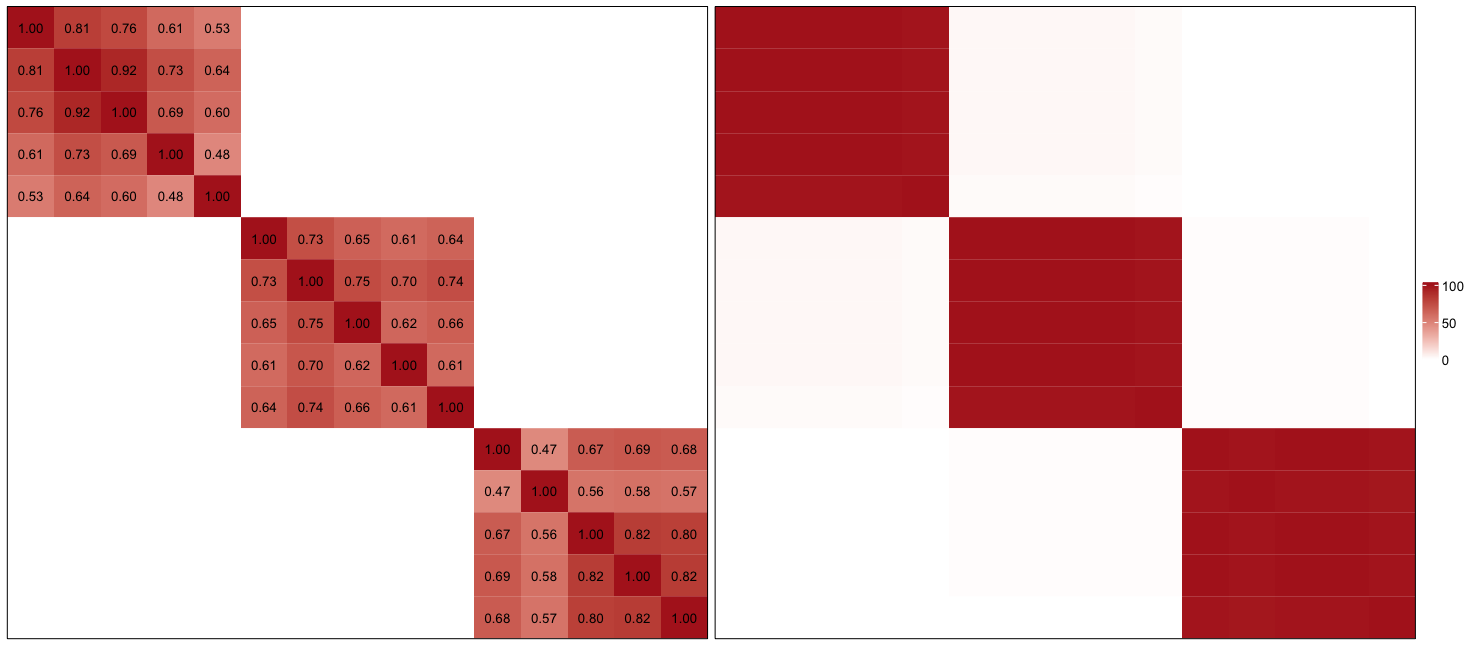
(a) Component 1

(b) Component 2

Figure 1: True correlation matrix of $\mathbf{X}$ (left); estimated correlation matrix of $\mathbf{X}$ (right) for each component in Setting 1.

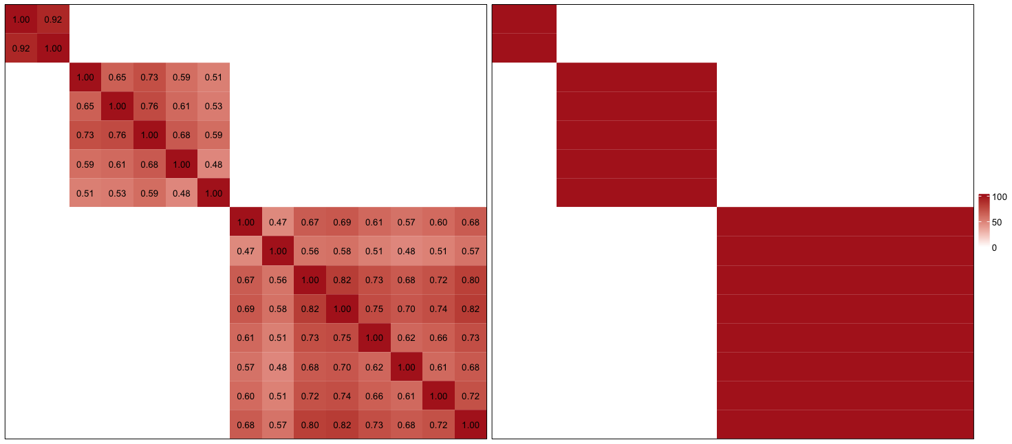
(a) Component 1

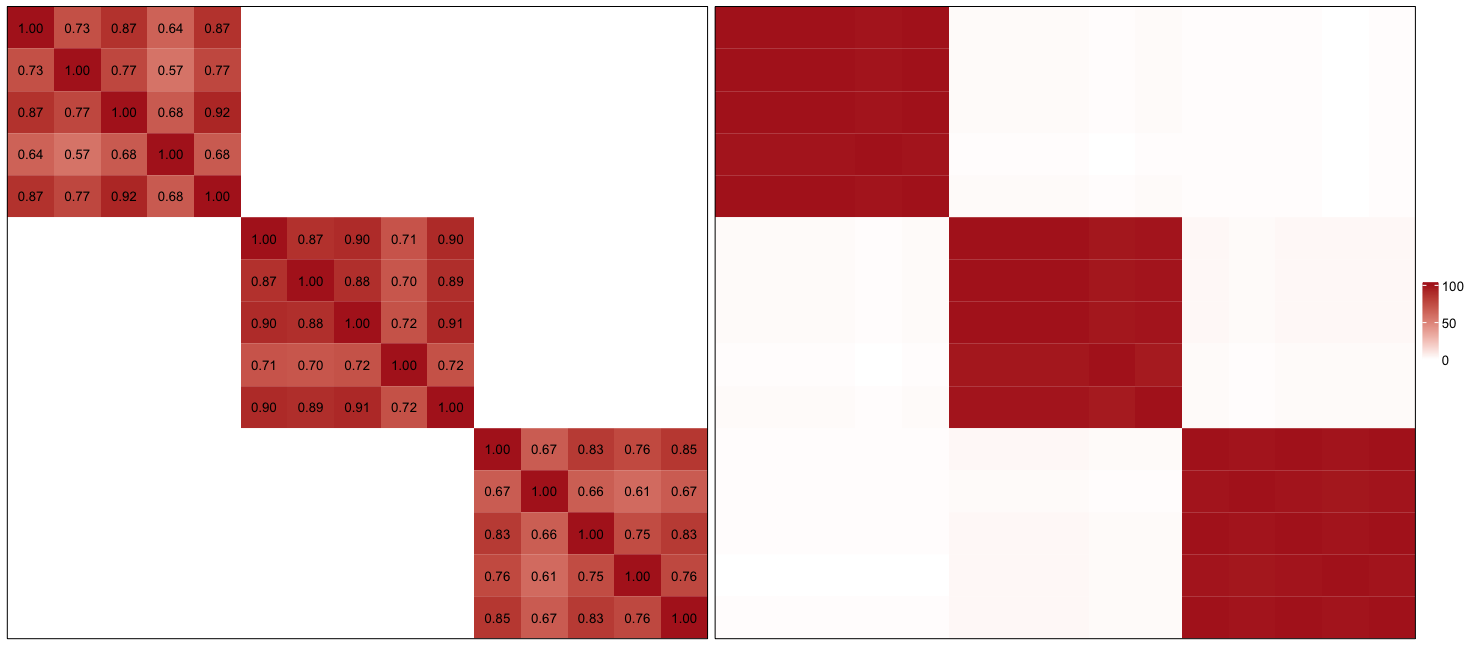
(b) Component 2

Figure 2: True correlation matrix of $\mathbf{X}$ (left); estimated correlation matrix of $\mathbf{X}$ (right) for each component in Setting 2.

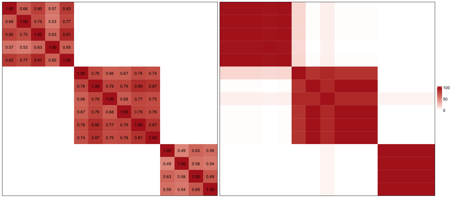
(a) Component 1

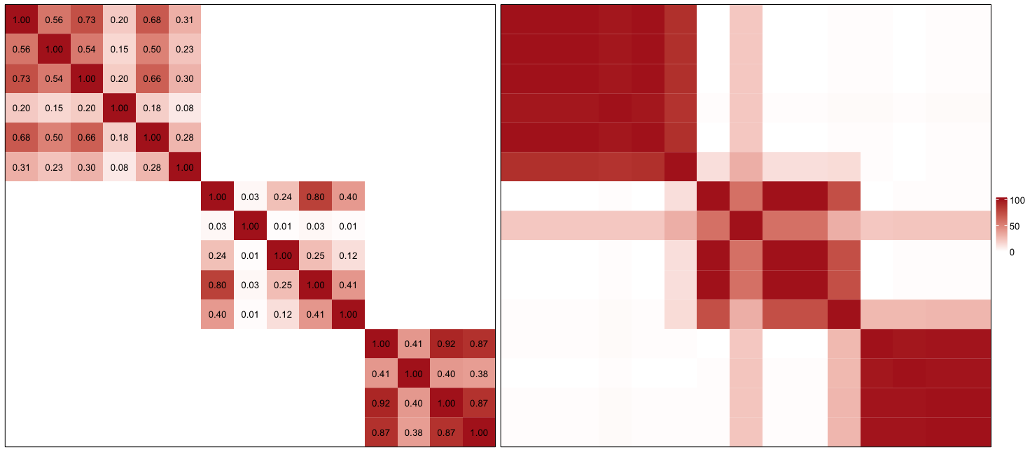
(b) Component 2

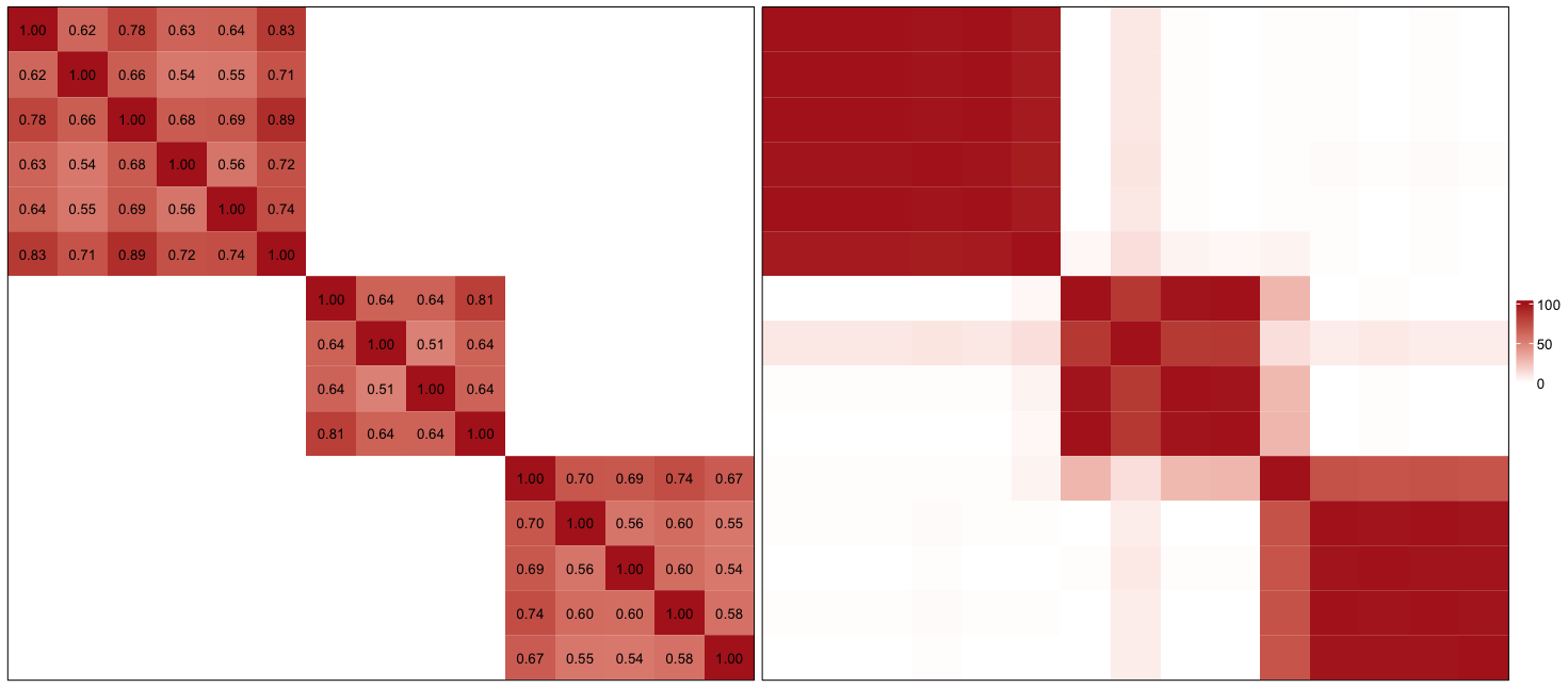
(c) Component 3

Figure 3: True correlation matrix of $\mathbf{X}$ (left); recovered groups of explanatory variables out of 100 times (right) for each component in Setting 3.

Regarding the recovery of component-specific parameters, Tables LABEL:simu1:setting1:MSE, LABEL:simu1:setting2:MSE, and LABEL:simu1:setting3:MSE in Appendix B display the entrywise average MSEs for Settings 1, 2, and 3, respectively, when the correct model was selected (according to ICL). The results indicate that the deviations from the true parameters are relatively small, suggesting that the model performs well in recovering component-specific parameters.

5.2 Simulation 2

In this simulation study, we investigated how varying the number of explanatory variables ($p=10,15,20,30$) and sample sizes ($N=500,750,1000$) affect the model’s performance. Specifically, we simulated 100 datasets considering the block structure as defined in Setting 2 of Simulation 1 and the parameters specified in Table LABEL:simu1:setting2:parameters. Table 3 provides the number of times the true model was selected by AIC, AIC3, BIC and ICL and the average ARI when the true model was selected across 100 datasets for various combinations of $p$ and $N$.
Most of the time the criteria can select the correct models and the average ARIs suggest perfect clustering recovered by the algorithm. BIC and ICL still perform better than AIC or AIC3, consistent with the observation in Simulation 1. The model selection suffers from the high dimensional explanatory variables. Given a fixed sample size, the criteria are more likely to identify the true components when the dimension is low.

		AIC(ARI)	AIC3(ARI)	BIC(ARI)	ICL(ARI)
$N$ = 500	$p$ = 10	98(1.00)	100(1.00)	100(1.00)	100(1.00)
	$p$ = 15	99(1.00)	100(1.00)	100(1.00)	100(1.00)
	$p$ = 20	91(1.00)	95(1.00)	97(1.00)	97(1.00)
	$p$ = 30	72(1.00)	82(1.00)	86(1.00)	86(1.00)
$N$ = 750	$p$ = 10	97(1.00)	100(1.00)	100(1.00)	100(1.00)
	$p$ = 15	93(1.00)	100(1.00)	100(1.00)	100(1.00)
	$p$ = 20	95(1.00)	100(1.00)	100(1.00)	100(1.00)
	$p$ = 30	72(1.00)	87(1.00)	90(1.00)	90(1.00)
$N$ = 1000	$p$ = 10	88(1.00)	100(1.00)	100(1.00)	100(1.00)
	$p$ = 15	84(1.00)	100(1.00)	100(1.00)	100(1.00)
	$p$ = 20	89(1.00)	97(1.00)	98(1.00)	98(1.00)
	$p$ = 30	67(1.00)	87(1.00)	90(1.00)	90(1.00)

Table 3: The number of times the correct model was selected of model criteria out of 100 datasets and ARI values (in brackets).

5.3 Simulation 3

Since in real data, the covariance/correlation matrix cannot be a perfect block diagonal matrix due to natural noise and overlap between explanatory variables, in this final simulation study, we aim to investigate how relatively small correlations between explanatory variables in different clusters (i.e. non-zero off-diagonal entries) influence the model’s performance. Here we set the off-diagonal entries to non-zero but without exceeding the correlations in diagonal blocks. To control the level of noise under $m$ while preserving the semi-positive definite correlation structure, we generate the covariance matrix $\mbox{\bm{$\Psi$}}_{g}$ in the following way:

1. Generate a symmetric matrix $\mbox{\bm{$\Phi$}}_{g}$ whose entry $(\mbox{\bm{$\Phi$}}_{g})_{ij}=U_{ij}\sqrt{(\mbox{\bm{$\Gamma$}}_{g})_{ii}(\mbox{\bm{$\Gamma$}}_{g})_{jj}}$, where $(\mbox{\bm{$\Gamma$}}_{g})_{ii}$, $(\mbox{\bm{$\Gamma$}}_{g})_{jj}$ are entries of $\mbox{\bm{$\Gamma$}}_{g}$, and $U_{ij}$ is drawn from a uniform distribution $\mathrm{U}(-m,m)$. We set $U_{ij}=U_{ji}$ for symmetry. Here $m>0$ is used as the level of noise.

2. Do eigendecomposition of $\mbox{\bm{$\Phi$}}_{g}=\mathbf{P}\mathbf{E}\mathbf{P}^{\prime}$ as $\Phi$ is symmetric. Here $\mathbf{P}$ is the matrix of eigenvectors and $\mathbf{E}$ is a diagonal matrix corresponding to eigenvalues. Also, we have $\mathbf{P}^{\prime}=\mathbf{P}^{-1}$.

3. Reconstruct $\widetilde{\mbox{\bm{$\Phi$}}}_{g}=\mathbf{P}\widetilde{\mathbf{E}}\mathbf{P}^{\prime}$ where the entry

   $$\widetilde{\mathbf{E}}_{ij}=\begin{cases}\mathbf{E}_{ij},\mathbf{E}_{ij}\geq 0\\ 0,\textrm{otherwise.}\end{cases}$$

4. Create $\mbox{\bm{$\Psi$}}_{g}$ whose entry $(\mbox{\bm{$\Psi$}}_{g})_{ij}$ is

   $$(\mbox{\bm{$\Psi$}}_{g})_{ij}=\begin{cases}1+(\widetilde{\mbox{\bm{$\Phi$}}}_{g})_{ii},i=j\\ (\widetilde{\mbox{\bm{$\Phi$}}}_{g})_{ij},\textrm{otherwise,}\\ \end{cases}$$

   which guarantees a positive definite correlation.

To see the effect of noise level $m$, we deploy two settings. In Setting 1, $m$ is $0.43$; in Setting 2, $m$ is $0.77$. Then we simulated 100 datasets with $G=2$ components, $M=5$ response variables, $p=20$ explanatory variables, $Q=3$ segments of explanatory variables and sample size $n=750$. The mixing proportion is $\pi=(0.6,0.4)$. We ran the AECM algorithm on each dataset with $G=1,2,3,4,5$ and $Q=1,2,3,4,5$, respectively.

The recovered segments/groups of explanatory variables are obtained for each dataset and summarised in Figure 4 and 5. The clustering of explanatory variables accurately captures the main structure of the true correlation matrix in both settings.

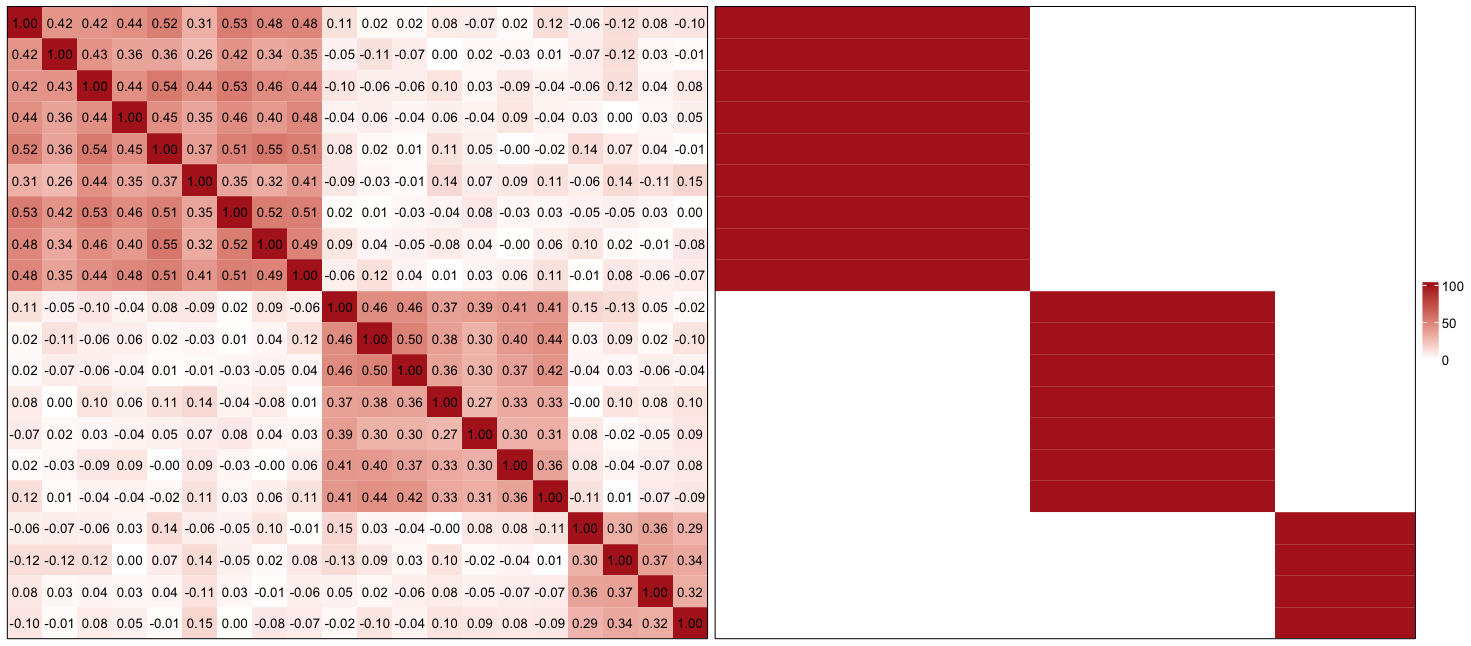
(A) Component 1

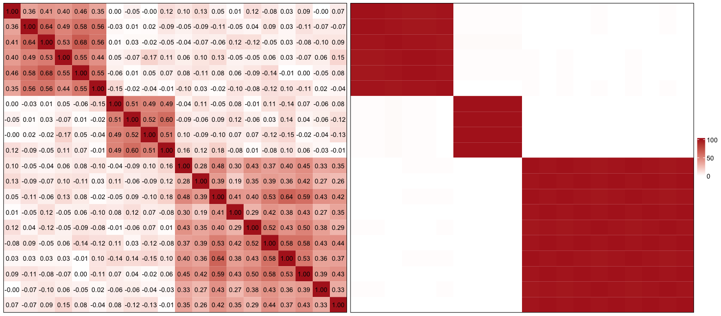
(B) Component 2

Figure 4: True correlation matrix of $\mathbf{X}$ (left); recovered groups of explanatory variables out of 100 times (right) for each component.

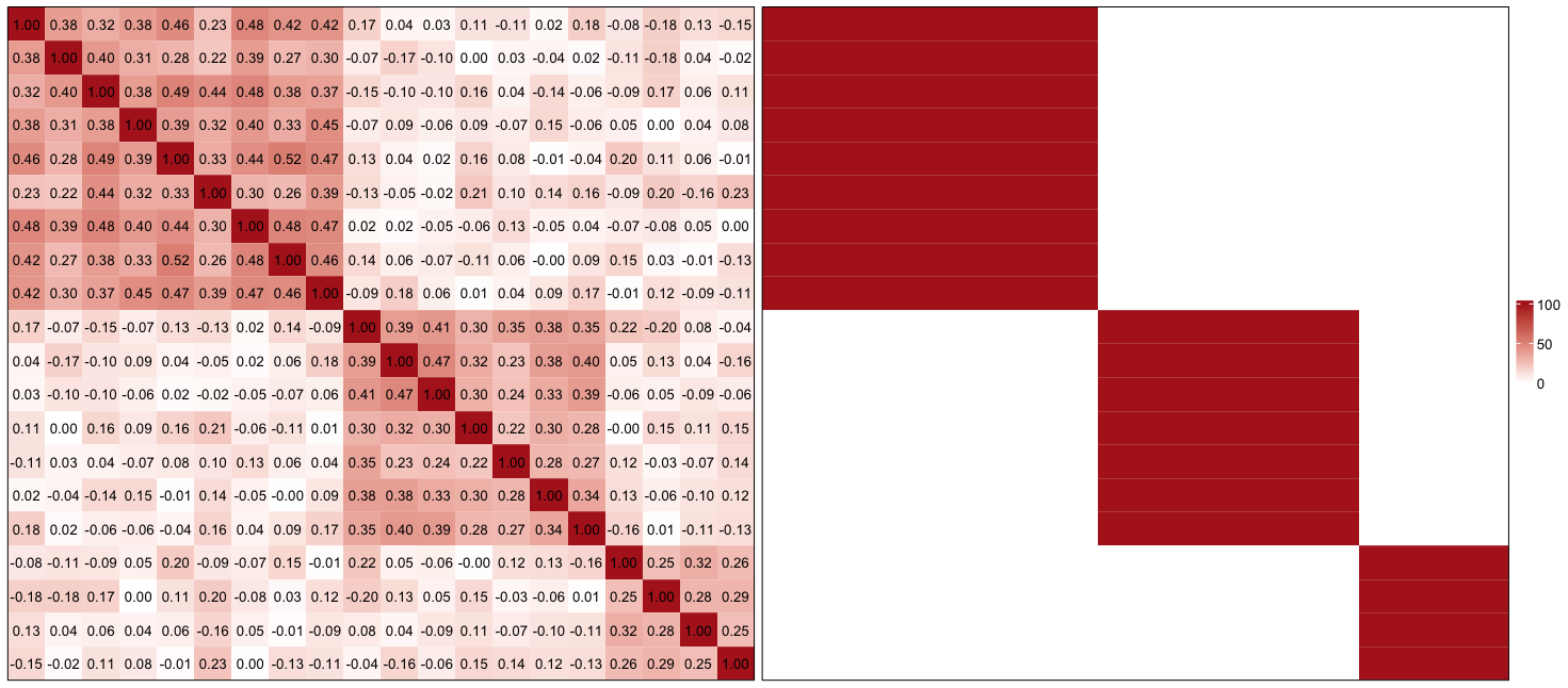
(A) Component 1

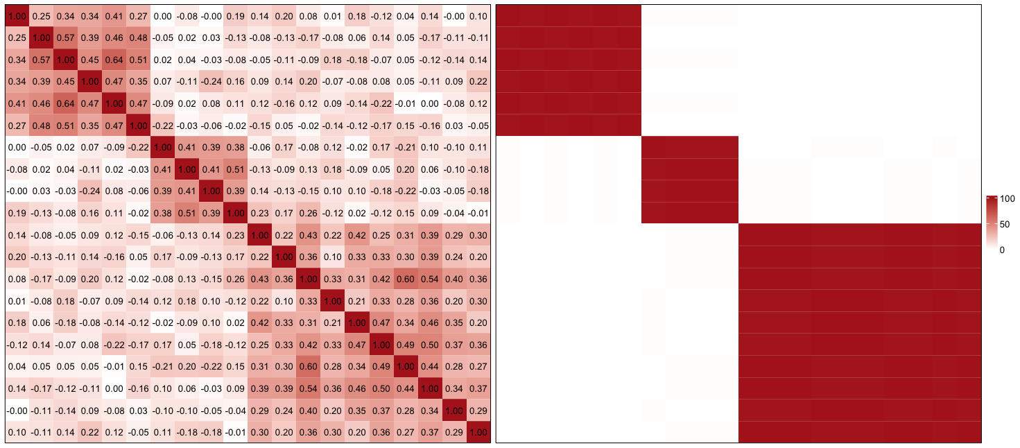
(B) Component 2

Figure 5: True correlation matrix of $\mathbf{X}$ (left); recovered groups of explanatory variables out of 100 times (right) for each component.

6 Crime data of communities within the United States

In this section, we start by performing an exploratory analysis of the real-world dataset named ‘Community and Crime Unnormalized’ from the UCI Machine Learning Repository. Subsequently, we apply the proposed model to the dataset and discuss the results obtained.

6.1 Exploratory data analysis

The crime dataset combines socioeconomic information of communities from the 1990 United States Census, law enforcement data from the 1990 Law Enforcement Management and Admin Stats survey, and crime data from the 1995 FBI UCR. Each dataset entry is an observation at the community level, including rates of different types of crime, population demographics, age structure, socio-economic status, etc. In this study, we focused exclusively on economic crimes ($M=3)$, including robberies, burglaries, and larcenies, among all types of offences. Additionally, we examined various community-level characteristics related to (a) general population demographics, (b) income and employment, and (c) housing. After excluding highly collinear socio-economic features, we considered the remaining $p=16$ socio-economic variables, encompassing $N$= 1901 communities (observations with missing records were excluded from the analysis). A brief overview of the variables included in the analysis is provided in Table 4. Skewed variables were log-transformed to meet the normality assumptions.

Type	General group	Varaible Name	Description
Responses Variables	Properties related crimes	Robberies	Number of robberies per 100,000 population
		Burglaries	Number of burglaries per 100,000 population
		Larcenies	Number of larcenies per 100,000 population
Explanatory variables	General Characteristics	pop
		pct_low_edu	Percentage of people 25 and over with less than a 9th grade education
	Income and Employment	pct_retire	Percentage with retirement income
		pct_wsocsec	Percentage with SSI
		pct_unemploy	Percentage of unemployment
		pct_wfarm	Percentage of households with farm or self employment income
		pct_employ_mfg	Percentage of people in manufacturing
		pct_employ_prof_serv	Percentage of people in professional services
	Housing related	pct_vacant_boarded	Percentage of vacant housing boarded up
		pct_vacant6up	Percentage of housing that has been vacant more than 6 months
		pct_hous_owner_occup	Percentage of households owner occupied
		own_hous_qrange	Q range of owner-occupied housing
		rent_qrange	Q range of rent housing
		med_rentpct_hous	Median rent as a percentage of household income
		med_own_costpct	Median owners cost as a percentage of household income for owners
		med_own_cost_pct_wo	Median owners cost as a percentage of household income for owners without a mortgage

Table 4: Details of the variables included in the analysis.

For a more comprehensive understanding of economic crimes, Figure 6 presents the distributions of log-transformed crime rates at the county level. As observed, the analysis of these distributions confirms significant heterogeneity in economic crimes across the US. The distribution of robberies has a quite clear pattern: we can observe the relatively high values on the West Coast and the Southeastern region, which hints at a decreasing trend from the coasts to the central and from the south to the north on the East Coast. Similarly, burglary rates follow a similar pattern, with higher numbers in California and Florida compared to a more uniform distribution across the rest of the US. Furthermore, the number of burglaries is much higher in Whatcom County of Washington compared to its adjacent region. The larcenies are the most frequent economic crimes of the three crimes we investigated. Most counties have a high rate of larceny, however, several exceptions can be found in the Northeast and the South. Larceny dominates the overall economic crime rate because of its high frequency. So, the pattern of overall crime rates is similar to larcenies.

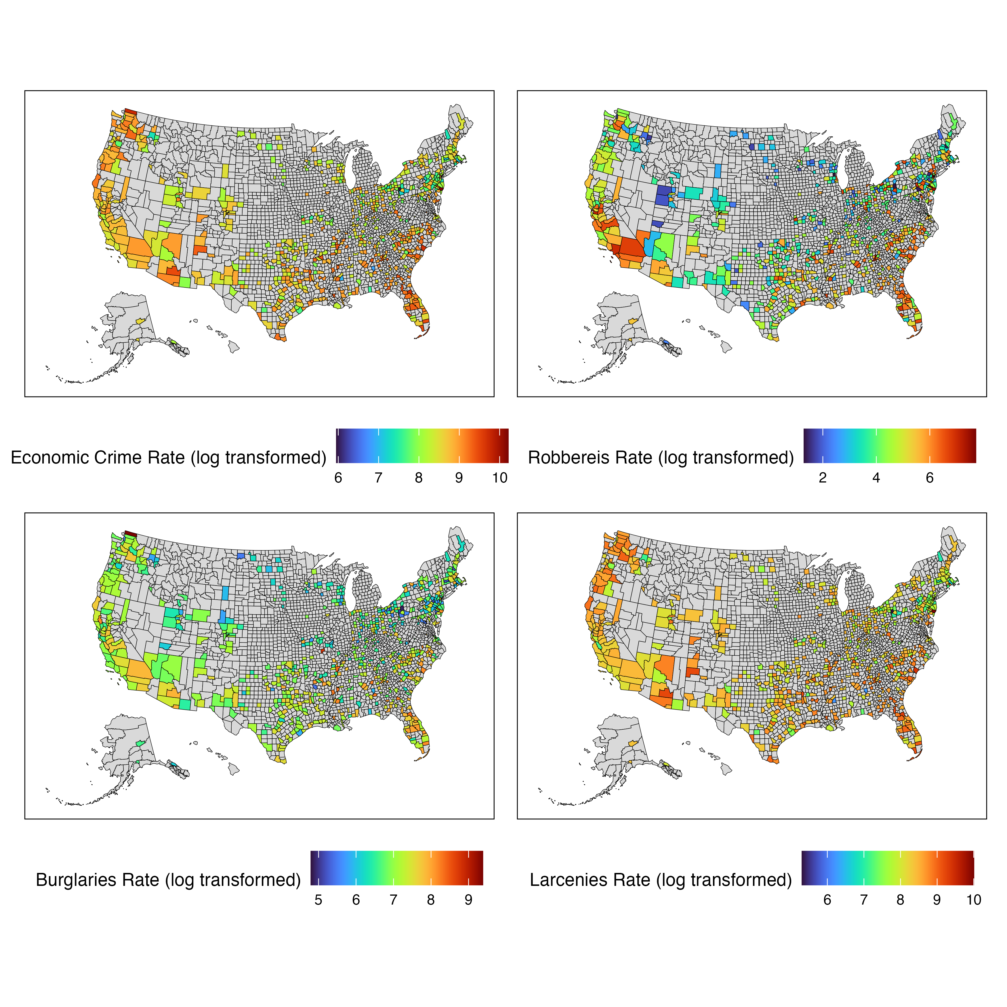
Figure 6: The distribution of log-transformed economic crime rates per 100k population at the county level.

6.2 Results from the MCWDFA Model

Driven by the well-known diverse crime landscape across communities in the United States, we aim to investigate how the $p=16$ socio-economic factors impact the $M=3$ crime rates. Specifically, our goal is twofold: first, to identify community groups with distinct effects of socio-economic factors on crime rates, and second, to determine if there are segments or groups of socio-economic factors that similarly influence economic crimes. We applied the proposed AECM algorithm with $G=1,2,\dots,10$ and $Q=1,2,\dots,10$ for ten times. The model with the highest ICL was selected ($G=6,Q=3$).

Figure 7(a) provides a visualization of the clustering results at the county level on the US map. The average crime rates of the estimated clusters are presented in Figure 7(b). To characterize the estimated clusters, we also use external county classification data provided by the Economic Research Service U.S. Department of Agriculture Economic Research Services (https://www.ers.usda.gov/data-products/county-typology-codes/) to better understand the socio-economic and geographic contexts of each cluster. We considered the following external variables: the economy types the counties depend on, whether the county is a retirement destination, the presence of persistent poverty, levels of education, employment rates, and significant housing stress. The characterization of the clusters based on these variables is summarized in Figure 7(c).

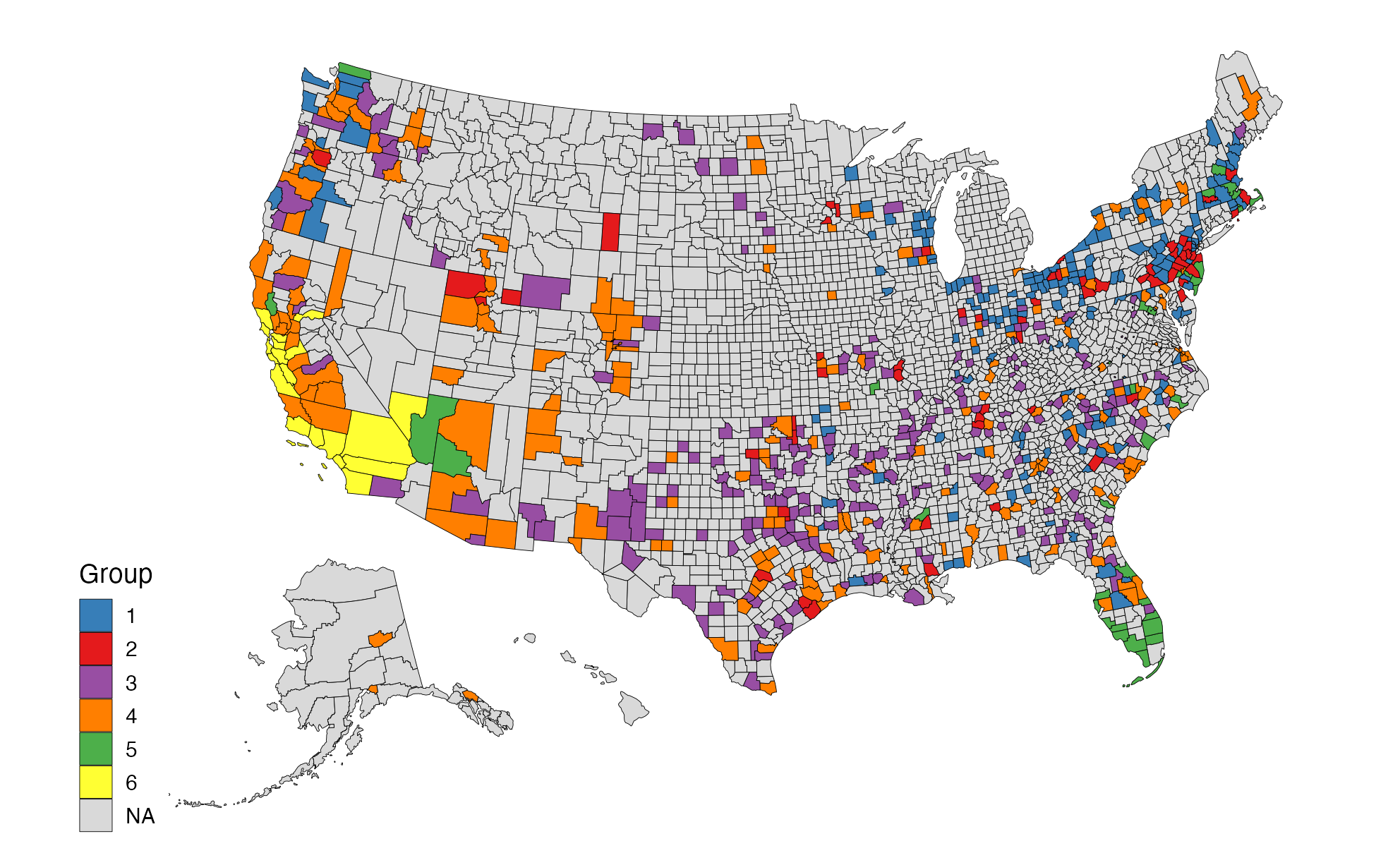
(a) Community clusters visualized at the county level on the US map

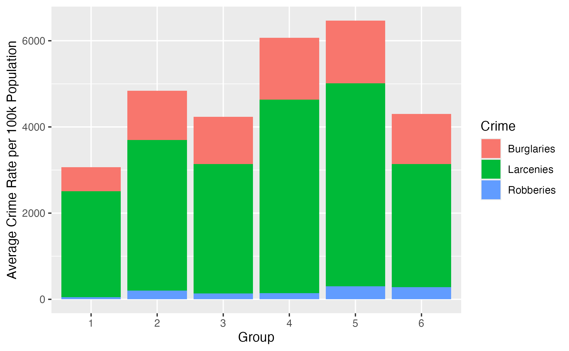
(b) Economic crime rates by clusters

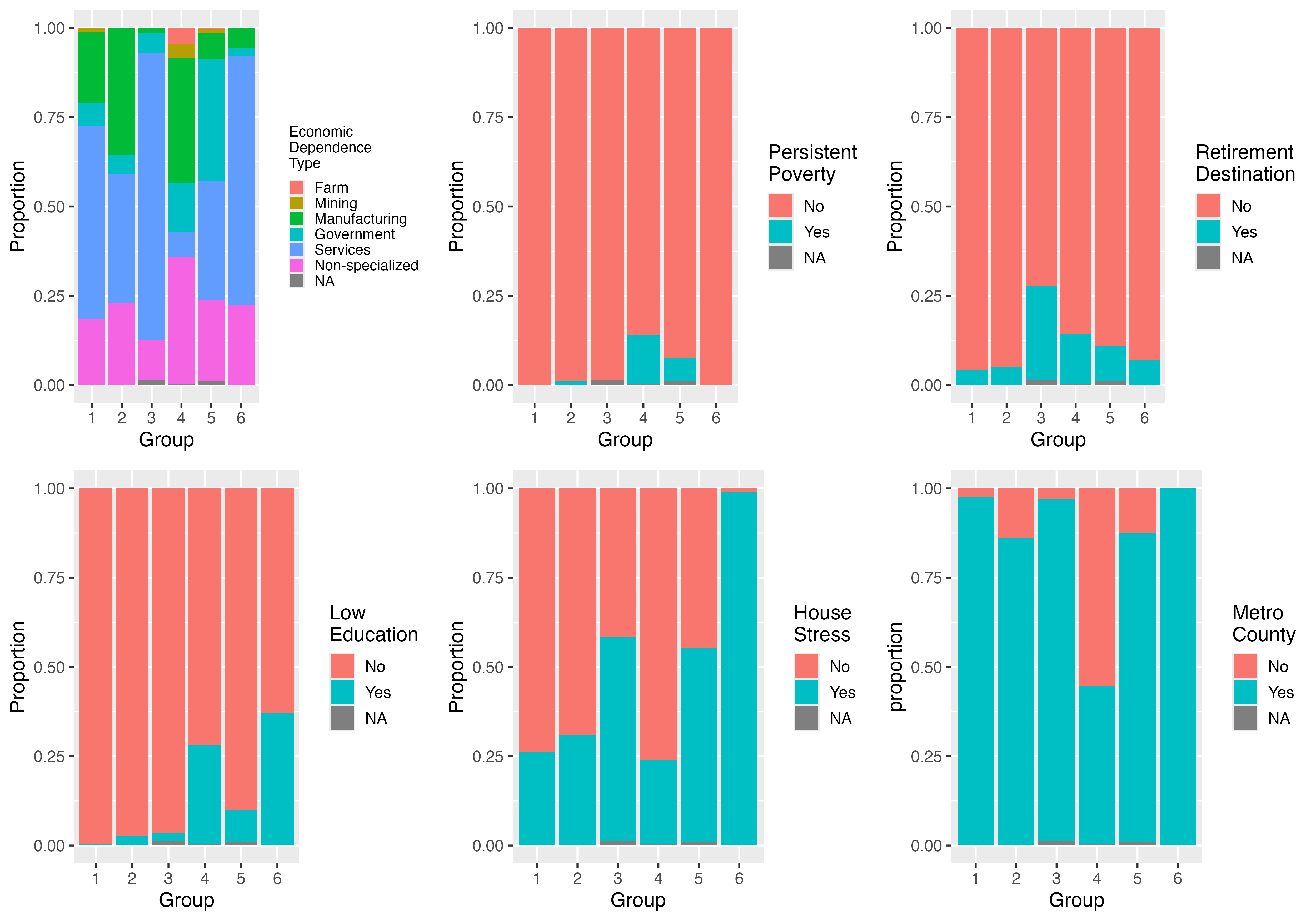
(c) Characteristics of the clusters

Figure 7: Clustering results at the county level: (a) visualization of clusters on the US map, (b) economic crime rates by clusters, and (c) characteristics of the clusters.

The main findings are summarized as follows. Counties in Cluster 1 and Cluster 2 are concentrated in the Northeastern. They differ mainly because of varying levels of crime: Cluster 2 has higher crime rates compared to Cluster 1, and Cluster 1 has the lowest overall crime rates. Cluster 2 has a higher proportion of manufacturing-dependent counties and lower services-dependent counties. Cluster 3, on the other hand, has the most retirement destinations, the highest proportion of services-dependent counties, fewer counties with persistent child poverty and they are almost all in metro counties. Cluster 4 and Cluster 5 both have high crime rates but differ significantly. Cluster 4 has the highest proportion of non-metro counties (likely rural), with persistent child poverty, low education, and a high proportion of manufacturing, farm and mining-dependent counties. In contrast, Cluster 5 has a high proportion of government-dependent counties, more counties with housing stress, and fewer counties with low education. Cluster 6 predominantly includes metropolitan counties in the western United States, particularly California and Nevada. It is characterized by average crime rates and the highest level of counties believed low education. This cluster primarily consists of service-dependent counties that face significant housing stress and does not include any counties experiencing persistent poverty. In summary, our results are consistent with established geographic and economic patterns, indicating that the composition of the clusters reflects meaningful geographic and economic distinctions.

Cluster 1		Cluster 2		Cluster 3
Factor 1:	Weight	Factor 1:	Weight	Factor 1:	Weight
pct_wsocsec	0.43	pct_wsocsec	0.83	pop	0.01
pct_retire	0.76	pct_retire	0.86	pct_low_edu	0.36
pct_employ_mfg	0.03	pct_low_edu	0.41	pct_unemploy	0.77
pct_hous_owner_occup	0.43	pct_unemploy	0.16	pct_vacant_boarded	0.35
Factor 2:		pct_employ_prof_serv	0.19	rent_qrange	0.10
pct_wfarm	0.01	Factor 2:		med_rentpct_hous	0.59
own_hous_qrange	0.58	pop	0.01	med_own_costpct	0.40
rent_qrange	0.76	pct_wfarm	0.10	med_own_cost_pct_wo	0.21
med_own_costpct	0.90	pct_hous_owner_occup	0.36	Factor 2:
med_own_cost_pct_wo	0.71	pct_vacant_boarded	0.20	pct_wfarm	0.19
Factor 3:		pct_vacant6up	0.40	pct_hous_owner_occup	0.42
pop	0.23	own_hous_qrange	0.69	pct_vacant6up	0.38
pct_low_edu	0.20	rent_qrange	1.03	Factor 3:
pct_unemploy	0.67	med_rentpct_hous	0.44	pct_wsocsec	0.44
pct_employ_prof_serv	0.18	med_own_costpct	0.60	pct_retire	0.59
pct_vacant_boarded	0.61	med_own_cost_pct_wo	0.53	pct_employ_mfg	0.02
pct_vacant6up	0.40	Factor 3:		pct_employ_prof_serv	0.30
med_rentpct_hous	0.44	pct_employ_mfg	0.47	own_hous_qrange	0.05
Cluster 4		Cluster 5		Cluster 6
Factor 1:	Weight	Factor 1:	Weight	Factor 1:	Weight
pct_wfarm	0.27	pct_wsocsec	1.39	pop	0.18
pct_employ_prof_serv	1.26	pct_retire	1.18	pct_low_edu	1.17
med_rentpct_hous	0.74	pct_low_edu	0.36	pct_unemploy	0.98
Factor 2:		pct_unemploy	0.35	pct_employ_mfg	0.35
own_hous_qrange	0.54	pct_hous_owner_occup	0.33	pct_vacant_boarded	0.47
rent_qrange	0.37	med_rentpct_hous	0.55	pct_vacant6up	0.12
med_own_costpct	0.24	Factor 2:		med_rentpct_hous	0.50
Factor 3:		pct_employ_mfg	0.10	med_own_costpct	0.14
pop	0.55	pct_vacant_boarded	0.17	med_own_cost_pct_wo	0.07
pct_wsocsec	0.46	pct_vacant6up	0.40	Factor 2:
pct_retire	0.17	med_own_costpct	0.14	pct_wsocsec	0.46
pct_low_edu	0.50	med_own_cost_pct_wo	1.15	pct_retire	0.71
pct_unemploy	0.39	Factor 3:		pct_hous_owner_occup	0.20
pct_employ_mfg	0.11	pop	0.03	Factor 3:
pct_hous_owner_occup	0.11	pct_wfarm	0.37	pct_wfarm	0.21
pct_vacant_boarded	0.86	pct_employ_prof_serv	0.63	pct_employ_prof_serv	0.42
pct_vacant6up	0.46	own_hous_qrange	1.06	own_hous_qrange	0.70
med_own_cost_pct_wo	0.36	rent_qrange	0.72	rent_qrange	0.35

Table 5: Weights $\mathbf{W}_{g}\mathbf{V}_{g}$ in $g=1,\dots,6$ for the explanatory variables. The three types of variables: General characteristics, Income and Employment, Housing.

From Table 5, it is possible to observe which explanatory variables form the factors and their associated weights $\mathbf{W}_{g}\mathbf{V}_{g}$ for each $g=1,\dots,6$. The latter allows us to evaluate the relative importance of each variable within the corresponding factor for each $g=1,\dots,6$. The three types of socio-economic variables — General Characteristics, Income and Employment, and Housing — are colored differently for clarity. As expected, depending on the community cluster, each factor is formed by different socio-economic variables which similarly predict the responses. In other words, each factor is not equivalent across community clusters. Thus, the factor has a different meaning for each community cluster and potentially can act differently on the responses. For example, Factor 1 in Cluster 1 differs from Factor 1 in other clusters, while Factor 1 in Cluster 3 has a similar meaning to Factor 1 in Cluster 6. Generally, the tendency is that the majority of socio-economic variables related to Housing cluster together in one or more clusters, such the percentages of vacant houses and vacant houses broadened over 6 months. The same is for socio-economic variables related to Income, such as the percentage of people with social security income and retired workers. Depending on the community cluster, the socio-economic variables related to General characteristics cluster either with a subset of Housing related socio-economic variables or a subset of Employment related socio-economic variables.

	$b_{1jm}w_{jj}v_{jq}$	Factor 1	Factor 2	Factor 3
Cluster 1	Robberies	-0.24	-0.1	0.4
	Burglaries	-0.15	-0.11	0.29
	Larcenies	-0.18	-0.26	0.04
Cluster 2	Robberies	0.23	-0.34	-0.13
	Burglaries	0.03	-0.12	-0.04
	Larcenies	0.11	-0.21	-0.06
Cluster 3	Robberies	0.31	-0.37	0.04
	Burglaries	0.22	-0.13	0.02
	Larcenies	0.04	-0.14	0.01
Cluster 4	Robberies	-0.31	0.17	0.62
	Burglaries	-0.14	0.05	0.29
	Larcenies	-0.17	0.03	0.11
Cluster 5	Robberies	0.11	-0.19	0
	Burglaries	0.12	-0.18	0.02
	Larcenies	0.03	-0.11	-0.04
Cluster 6	Robberies	0.53	-0.07	0.01
	Burglaries	0.07	-0.02	-0.08
	Larcenies	-0.15	0.04	-0.04

Table 6: Regression coefficients $\mathbf{B}_{1g}^{\prime}\mathbf{W}_{g}\mathbf{V}_{g}$ for $g=1,\dots,6$

Finally, Table 6 displays the regression coefficients in the reduced space computed as $\mathbf{B}_{1g}^{\prime}\mathbf{W}_{g}\mathbf{V}_{g}$ ($g=1,\dots,6$). For each crime, the highest coefficient (by absolute value) is highlighted: red for negative coefficients green for positive coefficients. From this table, we can observe, for instance, that within Cluster 3, Factor 2 appears to have the strongest negative impact on all responses, while within Cluster 5, Factor 3 appears to have no significant effects on any of the responses. Instead of working with various explanatory variables, we focus on the reduced space of latent factors. In the original space, we need to consider the effects of 16 variables in 6 different groups, which is a challenge for identifying patterns. Additionally, the correlations among the predictors are not taken into account. The disjoint factor structure provides a partition of variables, where the effects are the comprehensive impact of predictors in the groups. We can easily figure out how a factor affects the crime rates, and further investigate the variables related to the factor.
In community Cluster 1, both Factor 1 and Factor 2 decrease all responses, whereas a higher Factor 3 significantly raises all the responses, particularly Robberies and Burglaries. It is a reasonable result considering Factor 3 for Cluster 1 includes percentages of unemployment and vacant houses. For Cluster 2, Factor 2 and Factor 3 decrease the crime rates overall. Factor 1, including percentages of people retired, unemployed, or with low education or social security income, has the most positive effects on the responses. For Cluster 3, Factor 1 has the highest impact on the responses, while Factor 3 also positively influences them less significantly. Factor 2 decreases all crime rates and contains the percentage of the population with farming or self-employed income. Factor 2 also has the percentage of houses used by owners and the percentage of houses vacant for more than 6 months. Cluster 4 has the most non-metro counties and the most counties with persistent poverty and low education. Factor 3 significantly raises all the crime rates, and is related to population, retired, unemployed people, education level, social security income, percentage of vacant houses, and median owner cost of houses without a mortgage. Factor 2 also raises crime rates but is not comparable with Factor 3. Factor 1, related to the percentage of people with farming or self-employment income, the percentage of professional employees and the median rent level, impacts the crime rates to the opposite. Crime rates of Cluster 5 are mainly influenced by Factor 1 and Factor 2. Factor 1 is more about the level of retirement, unemployment, social security income and rent. A higher Factor 1 indicates higher crime rates. For Factor 2, on the opposite, a higher value may imply lower crime rates. Factor 2 is related to the group size of workers in manufacturing, vacant housing and the cost of owning a house. Cluster 6 is mainly associated with Factor 1, of which the effects differ in direction for Robberies and Larcenies. It looks like a higher level of population, low education, unemployment, rent and cost of housing, included in Factor 1, raises Robberies but lowers Larcenies.

7 Conclusion and discussions

The proposed MCWDFA extends CWFA in two ways: the multivariate responses and a disjoint factor analyzer. The multivariate assumption allows us to finish the analysis of multiple responses in one run. The disjoint factor assumption provides a more interpretable structure for latent factors. An AECM algorithm was developed for parameter recovery and clustering. A series of simulations were conducted to present the model’s performance under various scenarios. Three sets of simulations had different numbers of components and sizes of predictor groups. Our model has the ability to figure out the correct latent structures of datasets most of the time under the assessments of BIC and ICL. ARI also measured the clustering accuracies well. Then the performance under different sample sizes and numbers of covariates was tested. The model still presents the ability to recover the true number of components and classify subjects correctly, though the ability decreases as the data set has a higher dimensionality. Then we considered the model’s performance on datasets having a not perfect block diagonal matrix. We can see it correctly reveals the latent factors’ disjoint structure. Throughout the process, AIC, AIC3, BIC and ICL were used for model assessment but ICL showed a fairly better performance. In the real data analysis part, we thus adopted ICL as the measure to select the optimal model.

We applied the model to the United States’ economic crime data at the community level in the 1990s’. The economic crime rates are strongly associated with the local society structure such as population, economic type, education level, housing market and poverty. We expect to uncover the latent disjoint factors under the observed covariates and also the latent subgroups of communities sharing similar societal structures. The proposed method enables us to achieve the goal. However, the factors discovered by the proposed model need further exploration for a better interpretation, though the factors have been associated with much fewer covariates. The proposed model can also be applied to other data sets concerning clustering and latent interpretable factors. Students’ scores in multiple subjects with other information and patients’ laboratory assessments after treatment with demographics can be potential real scenarios.

The empirical findings confirm substantial heterogeneity among United States communities regarding the impact of socio-economic information on economic crime rates. Additionally, significant variations were observed among socio-economic features in terms of their predictive abilities for crimes across different community clusters. The interesting aspect of the model is that the groups of covariates are associated with factors that are constructed from disjoint variables (meaning a variable can only belong to one factor), thus the factors are easily interpretable, as are the associated regression coefficients. It is worth noting that the factors may potentially change meaning depending on the cluster.
The proposed CWDFA model: 1) Confirms substantial differences among US communities in the impact of socio-economic factors on economic crime rates, identifying clusters with similar structures 2) Helps us to discover groups of socio-economic covariates associated with disjoint factors easier to interpret, as the associated regression coefficients.
Some future directions include improving the model’s performance with high-dimension data sets. A sparse structure might be incorporated in the coefficients matrices. As our model considers only continuous numeric data, the extension to categorical and compositional data is of interest, which are widespread data types in the survey data and demographic data. Some model-based hypothesis testing techniques could also be developed.

Appendix A Parameters used for data generation in the simulation study.

Table 7: Pameters used for data generation in Setting 1

Parameter	Values
$\widetilde{\mathbf{B}}_{1}$	$\begin{pmatrix}-0.16&-0.75&0.75&-0.54&-0.58\\ 0.23&-0.46&-1.11&-0.02&-0.65\\ -0.21&-0.70&-0.67&-0.86&-0.07\\ -0.90&0.14&-1.23&-0.06&0.58\\ -0.04&-0.14&-0.03&-1.07&-1.28\\ -0.08&-0.56&-0.40&-0.91&0.03\\ -0.57&-1.17&-0.17&-1.07&-0.12\\ -0.02&-1.17&-0.94&-0.29&-0.58\\ -0.62&0.06&-0.30&-0.87&-0.40\\ -0.90&-0.76&-1.39&-0.21&-0.55\\ -0.85&-0.54&-1.09&0.29&-0.01\\ -0.00&-0.69&-0.40&-0.58&-0.25\\ -0.15&0.03&-0.82&-0.83&-0.27\\ -0.53&-0.49&-0.38&-0.90&-0.31\\ -0.81&-0.81&0.08&-0.86&-1.17\\ -0.80&-0.78&-0.53&-1.29&0.24\\ \end{pmatrix}$
$\widetilde{\mathbf{B}}_{2}$	$\begin{pmatrix}0.35&0.30&1.03&-1.56&-0.06\\ 1.09&-1.26&-0.80&-0.61&1.34\\ 0.30&-0.52&0.27&0.44&-0.54\\ 0.70&1.10&0.36&-1.40&1.07\\ -1.01&0.79&-0.35&0.83&0.71\\ -0.37&-0.52&-1.11&-0.79&0.08\\ 0.68&0.69&-0.08&0.79&0.02\\ -1.69&-0.16&0.24&0.72&2.02\\ -0.42&-0.00&-0.55&-0.79&-0.74\\ -0.11&0.92&0.34&-0.56&-0.81\\ -0.82&1.09&0.20&1.11&1.10\\ 0.14&-0.85&-0.40&0.72&-0.00\\ -0.78&1.48&-1.02&0.14&0.14\\ -0.31&-0.15&0.75&-0.19&-0.17\\ -1.06&0.84&0.86&-0.66&0.22\\ -0.13&-0.06&0.41&-0.51&-0.27\\ \end{pmatrix}$
$\mbox{\boldmath$\Sigma$}_{\mathbf{e}_{1}}$	$\begin{pmatrix}2.01&1.13&0.63&0.83&0.79\\ 1.13&1.83&0.97&0.81&0.50\\ 0.63&0.97&1.42&0.52&0.65\\ 0.83&0.81&0.52&1.55&0.74\\ 0.79&0.50&0.65&0.74&1.00\\ \end{pmatrix}$
$\mbox{\boldmath$\Sigma$}_{\mathbf{e}_{2}}$	$\begin{pmatrix}1.79&1.46&1.18&0.30&0.61\\ 1.46&3.64&2.12&0.88&0.99\\ 1.18&2.12&1.80&0.49&0.77\\ 0.30&0.88&0.49&1.00&0.04\\ 0.61&0.99&0.77&0.04&1.00\\ \end{pmatrix}$
$\mbox{\boldmath$\mu$}_{1}$	$\setcounter{MaxMatrixCols}{15}\begin{pmatrix}-2.57&-2.95&-2.54&-2.85&-2.40&-2.60&-2.69&-2.01&-2.86&-2.57&-2.09&-2.40&-2.52&-2.59&-2.60\\ \end{pmatrix}$
$\mbox{\boldmath$\mu$}_{2}$	$\setcounter{MaxMatrixCols}{15}\begin{pmatrix}3.19&3.74&3.19&3.61&3.62&3.77&3.16&3.75&3.28&3.98&3.24&3.57&3.37&3.34&3.53\\ \end{pmatrix}$
$\text{diag}(\mathbf{W}_{1})$	$\setcounter{MaxMatrixCols}{15}\begin{pmatrix}1.28&0.79&1.22&0.75&1.08&0.97&1.30&1.26&1.12&1.18&1.03&0.88&0.73&0.70&1.27\\ \end{pmatrix}$
$\text{diag}(\mathbf{W}_{2})$	$\setcounter{MaxMatrixCols}{15}\begin{pmatrix}1.64&0.88&1.62&0.80&1.18&0.93&1.44&0.72&0.83&1.47&0.94&1.83&0.95&1.90&1.70\\ \end{pmatrix}$
$\text{diag}(\mbox{\boldmath$\Psi$}_{1})$	$\setcounter{MaxMatrixCols}{15}\begin{pmatrix}0.96&0.48&0.72&0.85&0.29&0.02&0.28&0.29&0.24&0.69&0.87&0.57&0.29&0.69&0.38\\ \end{pmatrix}$
$\text{diag}(\mbox{\boldmath$\Psi$}_{2})$	$\setcounter{MaxMatrixCols}{15}\begin{pmatrix}0.50&0.67&0.32&0.14&0.77&0.19&0.18&0.09&0.67&0.99&0.09&0.28&0.69&0.34&0.51\\ \end{pmatrix}$

Table 8: Pameters used for data generation in Setting 2.

Parameter	Values
$\widetilde{\mathbf{B}}_{1}$	$\begin{pmatrix}-0.16&-0.75&0.75&-0.54&-0.58\\ 0.23&-0.46&-1.11&-0.02&-0.65\\ -0.21&-0.70&-0.67&-0.86&-0.07\\ -0.90&0.14&-1.23&-0.06&0.58\\ -0.04&-0.14&-0.03&-1.07&-1.28\\ -0.08&-0.56&-0.40&-0.91&0.03\\ -0.57&-1.17&-0.17&-1.07&-0.12\\ -0.02&-1.17&-0.94&-0.29&-0.58\\ -0.62&0.06&-0.30&-0.87&-0.40\\ -0.90&-0.76&-1.39&-0.21&-0.55\\ -0.85&-0.54&-1.09&0.29&-0.01\\ -0.00&-0.69&-0.40&-0.58&-0.25\\ -0.15&0.03&-0.82&-0.83&-0.27\\ -0.53&-0.49&-0.38&-0.90&-0.31\\ -0.81&-0.81&0.08&-0.86&-1.17\\ -0.80&-0.78&-0.53&-1.29&0.24\\ \end{pmatrix}$
$\widetilde{\mathbf{B}}_{2}$	$\begin{pmatrix}0.35&0.30&1.03&-1.56&-0.06\\ 1.09&-1.26&-0.80&-0.61&1.34\\ 0.30&-0.52&0.27&0.44&-0.54\\ 0.70&1.10&0.36&-1.40&1.07\\ -1.01&0.79&-0.35&0.83&0.71\\ -0.37&-0.52&-1.11&-0.79&0.08\\ 0.68&0.69&-0.08&0.79&0.02\\ -1.69&-0.16&0.24&0.72&2.02\\ -0.42&-0.00&-0.55&-0.79&-0.74\\ -0.11&0.92&0.34&-0.56&-0.81\\ -0.82&1.09&0.20&1.11&1.10\\ 0.14&-0.85&-0.40&0.72&-0.00\\ -0.78&1.48&-1.02&0.14&0.14\\ -0.31&-0.15&0.75&-0.19&-0.17\\ -1.06&0.84&0.86&-0.66&0.22\\ -0.13&-0.06&0.41&-0.51&-0.27\\ \end{pmatrix}$
$\mbox{\boldmath$\Sigma$}_{\mathbf{e}_{1}}$	$\begin{pmatrix}2.01&1.13&0.63&0.83&0.79\\ 1.13&1.83&0.97&0.81&0.50\\ 0.63&0.97&1.42&0.52&0.65\\ 0.83&0.81&0.52&1.55&0.74\\ 0.79&0.50&0.65&0.74&1.00\\ \end{pmatrix}$
$\mbox{\boldmath$\Sigma$}_{\mathbf{e}_{2}}$	$\begin{pmatrix}1.79&1.46&1.18&0.30&0.61\\ 1.46&3.64&2.12&0.88&0.99\\ 1.18&2.12&1.80&0.49&0.77\\ 0.30&0.88&0.49&1.00&0.04\\ 0.61&0.99&0.77&0.04&1.00\\ \end{pmatrix}$
$\mbox{\boldmath$\mu$}_{1}$	$\setcounter{MaxMatrixCols}{15}\begin{pmatrix}-2.57&-2.95&-2.54&-2.85&-2.40&-2.60&-2.69&-2.01&-2.86&-2.57&-2.09&-2.40&-2.52&-2.59&-2.60\\ \end{pmatrix}$
$\mbox{\boldmath$\mu$}_{2}$	$\setcounter{MaxMatrixCols}{15}\begin{pmatrix}3.19&3.74&3.19&3.61&3.62&3.77&3.16&3.75&3.28&3.98&3.24&3.57&3.37&3.34&3.53\\ \end{pmatrix}$
$\text{diag}(\mathbf{W}_{1})$	$\setcounter{MaxMatrixCols}{15}\begin{pmatrix}1.28&0.79&1.22&0.75&1.08&0.97&1.30&1.26&1.12&1.18&1.03&0.88&0.73&0.70&1.27\\ \end{pmatrix}$
$\text{diag}(\mathbf{W}_{2})$	$\setcounter{MaxMatrixCols}{15}\begin{pmatrix}1.64&0.88&1.62&0.80&1.18&0.93&1.44&0.72&0.83&1.47&0.94&1.83&0.95&1.90&1.70\\ \end{pmatrix}$
$\text{diag}(\mbox{\boldmath$\Psi$}_{1})$	$\setcounter{MaxMatrixCols}{15}\begin{pmatrix}0.96&0.48&0.72&0.85&0.29&0.02&0.28&0.29&0.24&0.69&0.87&0.57&0.29&0.69&0.38\\ \end{pmatrix}$
$\text{diag}(\mbox{\boldmath$\Psi$}_{2})$	$\setcounter{MaxMatrixCols}{15}\begin{pmatrix}0.50&0.67&0.32&0.14&0.77&0.19&0.18&0.09&0.67&0.99&0.09&0.28&0.69&0.34&0.51\\ \end{pmatrix}$

Table 9: Pameters used for data generation in Setting 3.

Parameter	Values
$\widetilde{\mathbf{B}}_{1}$	$\begin{pmatrix}-0.55&-0.71&-0.31&-0.15&-1.11&0.44&-0.15&-1.10&-0.51&-0.12\\ 0.09&-0.55&1.14&-0.11&-0.50&-0.82&-0.09&-0.24&-0.87&0.27\\ 0.68&-0.18&-0.63&0.05&-0.57&0.33&-1.53&-0.55&-1.22&0.43\\ 0.17&-0.47&-0.57&-0.49&0.35&-0.07&-0.20&-0.68&0.44&-1.60\\ -0.67&0.31&-0.83&0.06&1.03&-0.15&-0.02&-0.11&-0.93&0.50\\ 0.38&0.28&0.29&-1.04&-0.93&-0.66&-0.35&0.42&0.30&-0.12\\ -0.01&-0.09&-0.36&-0.56&0.40&-0.99&-0.01&-0.91&-0.33&-1.08\\ -0.24&-1.06&-0.02&-1.04&0.31&-0.30&-0.15&0.17&0.69&0.31\\ 0.35&-0.76&-0.84&-0.07&-0.43&-1.27&0.41&-0.37&-0.36&0.66\\ -0.51&0.10&0.06&-0.40&0.09&-0.44&0.04&-0.66&-0.42&-1.15\\ -0.70&-0.60&-1.19&-0.09&-0.31&0.64&-0.27&-0.87&-0.87&-1.46\\ -0.83&-0.07&-0.66&0.51&0.29&-0.64&0.49&0.23&0.30&0.06\\ 0.17&-0.29&-0.21&-0.16&0.21&0.26&-0.81&0.27&-0.09&-0.55\\ -0.01&0.20&-0.74&-0.47&0.11&-0.28&0.38&-0.85&-0.24&-0.83\\ -0.52&0.00&-0.26&-0.55&0.07&0.27&-0.01&-0.28&0.11&0.38\\ -0.77&-0.61&0.56&-0.78&-1.14&-0.82&-0.40&0.08&-0.58&0.26\\ \end{pmatrix}$
$\widetilde{\mathbf{B}}_{2}$	$\begin{pmatrix}0.13&1.01&0.76&-0.37&0.69&-1.40&-0.22&0.32&1.15&-1.15\\ 0.47&-0.41&1.31&-0.96&0.66&-0.85&-0.49&0.52&0.54&1.21\\ 0.37&0.10&0.08&0.07&-0.77&-0.71&-0.12&0.93&0.71&0.04\\ 0.44&-0.14&0.65&-0.09&-1.10&-0.78&0.74&-0.69&1.13&-0.01\\ -0.31&-0.86&-0.42&-1.09&0.29&1.15&0.14&-1.03&-0.63&-0.77\\ 1.08&1.12&1.20&-0.57&-0.36&-0.01&-0.26&1.09&-0.72&-1.11\\ -0.12&0.35&-0.92&0.22&-0.26&1.24&-0.35&0.50&-0.73&-0.90\\ -0.85&-0.23&-0.44&0.18&-0.15&-0.18&0.34&-0.54&0.76&-0.78\\ -0.69&1.51&-1.23&0.52&-0.03&0.34&0.48&-0.83&1.09&-1.67\\ 0.72&-0.54&0.47&-0.54&-0.70&-0.89&-0.70&-2.19&-0.38&-0.05\\ -0.13&0.78&0.80&0.01&-1.54&0.81&-0.10&-0.58&0.28&0.37\\ -0.43&0.66&0.21&-1.22&1.83&0.11&0.25&0.43&0.02&0.91\\ -1.04&0.23&0.46&0.78&-0.03&-0.69&1.49&-1.21&0.16&0.06\\ 0.65&-0.48&-0.44&-0.76&-0.27&0.95&-0.86&0.48&0.30&-0.05\\ 0.06&-0.71&-1.86&0.27&-0.11&-1.36&-0.11&0.02&-1.23&-2.24\\ 0.37&-1.28&0.27&-0.46&0.03&0.82&-1.38&-1.03&-0.34&-0.63\\ \end{pmatrix}$
$\widetilde{\mathbf{B}}_{3}$	$\begin{pmatrix}-1.74&1.52&-1.76&0.83&-0.04&0.67&0.84&-0.13&0.10&1.26\\ -0.16&-1.59&0.82&0.99&1.08&-1.87&0.17&0.07&-0.86&-0.27\\ -0.42&0.06&0.44&0.02&0.41&0.44&0.14&-1.40&-0.42&-1.62\\ -0.11&0.30&-1.21&0.02&0.29&1.17&-1.36&-0.73&0.50&-1.33\\ -0.44&0.84&0.13&-0.36&1.62&0.13&-1.53&1.69&0.35&1.08\\ -0.56&-0.06&1.10&-0.33&-0.98&0.29&0.12&0.49&-1.15&-0.47\\ -0.41&-1.60&-0.68&-0.73&-0.49&-1.28&-0.05&1.77&-0.97&0.64\\ 0.20&1.08&-0.29&0.71&-0.44&-1.28&0.42&1.31&-0.25&0.04\\ 0.57&0.43&0.66&-1.42&-0.15&-1.82&0.76&-1.13&0.38&-0.22\\ -0.69&-0.00&-1.14&0.21&0.04&-0.02&-0.47&-0.26&-1.74&2.28\\ -1.40&0.64&-0.37&-1.60&-2.22&-1.40&0.36&0.35&-0.38&-0.84\\ -1.33&-0.90&-1.25&-1.77&0.65&-0.77&0.49&-0.72&-1.39&-0.61\\ -0.43&0.46&-0.28&0.16&-2.36&1.39&-2.95&-0.49&0.58&-1.38\\ 0.69&0.76&0.25&-1.51&-0.91&1.47&-0.50&1.01&-0.65&0.54\\ 0.19&-0.13&1.01&0.39&-2.12&0.52&0.29&-0.45&-1.41&1.05\\ 0.03&0.71&-0.41&0.22&-0.35&-0.19&0.55&-1.72&-1.46&0.13\\ \end{pmatrix}$
$\mbox{\boldmath$\Sigma$}_{\mathbf{e}_{1}}$	$\begin{pmatrix}5.02&3.34&3.40&2.44&1.87&2.49&1.60&1.70&1.09&0.92\\ 3.34&3.49&2.53&1.59&1.87&1.91&0.99&0.76&0.84&0.64\\ 3.40&2.53&4.13&2.19&2.17&2.10&1.82&1.56&0.31&0.74\\ 2.44&1.59&2.19&2.84&0.90&1.37&0.98&1.66&0.44&0.76\\ 1.87&1.87&2.17&0.90&2.77&1.81&1.06&0.23&0.19&0.02\\ 2.49&1.91&2.10&1.37&1.81&2.73&1.49&0.78&1.01&0.10\\ 1.60&0.99&1.82&0.98&1.06&1.49&1.77&0.99&0.66&0.47\\ 1.70&0.76&1.56&1.66&0.23&0.78&0.99&1.77&0.36&0.88\\ 1.09&0.84&0.31&0.44&0.19&1.01&0.66&0.36&1.11&0.33\\ 0.92&0.64&0.74&0.76&0.02&0.10&0.47&0.88&0.33&1.00\\ \end{pmatrix}$
$\mbox{\boldmath$\Sigma$}_{\mathbf{e}_{2}}$	$\begin{pmatrix}4.55&3.12&2.18&2.65&2.37&2.82&1.90&2.11&1.53&0.79\\ 3.12&4.06&3.03&2.32&2.40&1.92&0.91&1.18&0.94&0.72\\ 2.18&3.03&3.65&1.92&2.19&1.48&0.65&0.59&0.32&0.06\\ 2.65&2.32&1.92&3.13&1.71&2.34&1.54&2.08&1.52&0.83\\ 2.37&2.40&2.19&1.71&3.20&2.48&1.63&1.25&0.62&0.69\\ 2.82&1.92&1.48&2.34&2.48&3.05&1.98&1.99&1.28&0.94\\ 1.90&0.91&0.65&1.54&1.63&1.98&2.25&1.77&1.00&0.55\\ 2.11&1.18&0.59&2.08&1.25&1.99&1.77&2.58&1.66&0.83\\ 1.53&0.94&0.32&1.52&0.62&1.28&1.00&1.66&1.74&0.86\\ 0.79&0.72&0.06&0.83&0.69&0.94&0.55&0.83&0.86&1.00\\ \end{pmatrix}$
$\mbox{\boldmath$\Sigma$}_{\mathbf{e}_{3}}$	$\begin{pmatrix}2.92&1.73&1.24&1.06&0.68&1.10&0.91&1.21&0.87&0.63\\ 1.73&3.65&1.65&2.20&0.91&1.52&1.12&0.27&0.16&0.14\\ 1.24&1.65&2.12&1.21&0.97&1.48&0.31&0.54&0.32&0.01\\ 1.06&2.20&1.21&3.03&1.09&2.21&1.38&1.22&0.31&0.23\\ 0.68&0.91&0.97&1.09&1.46&1.13&0.58&0.48&0.26&0.08\\ 1.10&1.52&1.48&2.21&1.13&2.89&1.27&1.39&0.81&0.15\\ 0.91&1.12&0.31&1.38&0.58&1.27&1.91&1.07&0.16&0.91\\ 1.21&0.27&0.54&1.22&0.48&1.39&1.07&2.18&0.81&0.81\\ 0.87&0.16&0.32&0.31&0.26&0.81&0.16&0.81&1.01&0.11\\ 0.63&0.14&0.01&0.23&0.08&0.15&0.91&0.81&0.11&1.00\\ \end{pmatrix}$
$\mbox{\boldmath$\mu$}_{1}$	$\setcounter{MaxMatrixCols}{15}\begin{pmatrix}-0.61&-0.07&0.08&0.08&-0.68&-0.69&0.06&-0.67&0.23&-0.67&0.23&-0.20&-0.57&0.08&-0.02\\ \end{pmatrix}$
$\mbox{\boldmath$\mu$}_{2}$	$\setcounter{MaxMatrixCols}{15}\begin{pmatrix}1.71&0.95&0.80&1.46&1.41&1.20&0.95&0.96&1.28&1.61&1.17&0.77&1.50&0.81&1.17\\ \end{pmatrix}$
$\mbox{\boldmath$\mu$}_{3}$	$\setcounter{MaxMatrixCols}{15}\begin{pmatrix}2.82&2.55&2.87&2.41&2.39&3.14&3.13&2.67&3.07&2.55&2.50&2.91&2.28&2.83&2.90\\ \end{pmatrix}$
$\text{diag}(\mathbf{W}_{1})$	$\setcounter{MaxMatrixCols}{15}\begin{pmatrix}1.28&0.79&1.22&0.75&1.08&0.97&1.30&1.26&1.12&1.18&1.03&0.88&0.73&0.70&1.27\\ \end{pmatrix}$
$\text{diag}(\mathbf{W}_{2})$	$\setcounter{MaxMatrixCols}{15}\begin{pmatrix}1.45&0.28&1.41&0.16&0.74&0.35&1.14&0.02&0.20&1.19&0.37&1.74&0.39&1.85&1.54\\ \end{pmatrix}$
$\text{diag}(\mathbf{W}_{3})$	$\setcounter{MaxMatrixCols}{15}\begin{pmatrix}1.00&1.00&1.00&1.00&1.00&1.00&1.00&1.00&1.00&1.00&1.00&1.00&1.00&1.00&1.00\\ \end{pmatrix}$
$\text{diag}(\mbox{\boldmath$\Psi$}_{1})$	$\setcounter{MaxMatrixCols}{15}\begin{pmatrix}0.61&0.36&0.21&0.69&0.07&0.52&0.19&0.78&0.56&0.16&0.20&0.67&0.65&0.18&0.86\\ \end{pmatrix}$
$\text{diag}(\mbox{\boldmath$\Psi$}_{2})$	$\setcounter{MaxMatrixCols}{15}\begin{pmatrix}0.68&0.11&0.85&0.42&0.34&0.87&0.38&0.61&0.47&0.29&0.54&0.23&0.70&0.32&0.53\\ \end{pmatrix}$
$\text{diag}(\mbox{\boldmath$\Psi$}_{3})$	$\setcounter{MaxMatrixCols}{15}\begin{pmatrix}0.37&0.88&0.21&0.81&0.75&0.05&0.23&0.96&0.97&0.24&0.16&0.77&0.80&0.56&0.90\\ \end{pmatrix}$

Appendix B Component-specific parameters recovery

Table 10: The average MSE of parameters when the correct model was selected (ICL) in Setting 1.

Parameter	Mean squared Error
$\widetilde{\mathbf{B}}_{1}$	$\begin{pmatrix}0.23&0.18&0.11&0.19&0.14\\ 0.01&0.01&0.00&0.01&0.00\\ 0.01&0.01&0.01&0.01&0.01\\ 0.01&0.01&0.01&0.01&0.00\\ 0.01&0.01&0.01&0.01&0.00\\ 0.02&0.02&0.01&0.01&0.01\\ 0.06&0.05&0.05&0.06&0.03\\ 0.02&0.02&0.01&0.02&0.01\\ 0.02&0.01&0.01&0.01&0.01\\ 0.02&0.02&0.01&0.01&0.01\\ 0.01&0.01&0.01&0.01&0.00\\ 0.01&0.01&0.01&0.01&0.01\\ 0.01&0.01&0.01&0.01&0.01\\ 0.02&0.02&0.01&0.01&0.01\\ 0.01&0.01&0.01&0.01&0.01\\ 0.01&0.01&0.01&0.01&0.01\\ \end{pmatrix}$
$\widetilde{\mathbf{B}}_{2}$	$\begin{pmatrix}1.41&2.87&1.28&0.82&0.71\\ 0.01&0.03&0.01&0.01&0.01\\ 0.01&0.03&0.01&0.01&0.01\\ 0.03&0.05&0.02&0.01&0.01\\ 0.05&0.11&0.06&0.04&0.03\\ 0.01&0.03&0.01&0.01&0.01\\ 0.04&0.09&0.04&0.02&0.02\\ 0.03&0.08&0.04&0.02&0.02\\ 0.09&0.18&0.09&0.05&0.05\\ 0.01&0.03&0.02&0.01&0.01\\ 0.01&0.02&0.01&0.01&0.01\\ 0.11&0.22&0.11&0.04&0.04\\ 0.02&0.05&0.03&0.01&0.02\\ 0.01&0.03&0.01&0.01&0.01\\ 0.02&0.04&0.02&0.01&0.01\\ 0.01&0.03&0.01&0.01&0.01\\ \end{pmatrix}$
$\mbox{\boldmath$\Sigma$}_{\mathbf{e}_{1}}$	$\begin{pmatrix}0.03&0.02&0.01&0.01&0.01\\ 0.02&0.03&0.02&0.01&0.01\\ 0.01&0.02&0.02&0.01&0.01\\ 0.01&0.01&0.01&0.02&0.01\\ 0.01&0.01&0.01&0.01&0.01\\ \end{pmatrix}$
$\mbox{\boldmath$\Sigma$}_{\mathbf{e}_{2}}$	$\begin{pmatrix}0.05&0.05&0.03&0.01&0.01\\ 0.05&0.20&0.07&0.03&0.04\\ 0.03&0.07&0.04&0.01&0.02\\ 0.01&0.03&0.01&0.02&0.00\\ 0.01&0.04&0.02&0.00&0.02\\ \end{pmatrix}$
$\mbox{\boldmath$\mu$}_{1}$	$\setcounter{MaxMatrixCols}{15}\begin{pmatrix}0.01&0.00&0.01&0.01&0.01&0.00&0.01&0.01&0.01&0.01&0.01&0.00&0.00&0.00&0.01\\ \end{pmatrix}$
$\mbox{\boldmath$\mu$}_{2}$	$\setcounter{MaxMatrixCols}{15}\begin{pmatrix}0.01&0.01&0.01&0.00&0.01&0.01&0.01&0.00&0.01&0.01&0.01&0.02&0.01&0.02&0.02\\ \end{pmatrix}$
$\text{diag}(\mathbf{W}_{1})$	$\setcounter{MaxMatrixCols}{15}\begin{pmatrix}0.02&0.00&0.00&0.00&0.00&0.00&0.00&0.02&0.00&0.02&0.00&0.01&0.01&0.00&0.00\\ \end{pmatrix}$
$\text{diag}(\mathbf{W}_{2})$	$\setcounter{MaxMatrixCols}{15}\begin{pmatrix}0.03&0.01&0.06&0.00&0.01&0.01&0.01&0.01&0.00&0.03&0.02&0.01&0.03&0.09&0.03\\ \end{pmatrix}$
$\text{diag}(\mbox{\boldmath$\Psi$}_{1})$	$\setcounter{MaxMatrixCols}{15}\begin{pmatrix}0.03&0.00&0.00&0.00&0.00&0.00&0.00&0.02&0.00&0.03&0.00&0.01&0.00&0.00&0.00\\ \end{pmatrix}$
$\text{diag}(\mbox{\boldmath$\Psi$}_{2})$	$\setcounter{MaxMatrixCols}{15}\begin{pmatrix}0.08&0.01&0.22&0.00&0.01&0.01&0.00&0.01&0.00&0.06&0.02&0.00&0.04&0.40&0.07\\ \end{pmatrix}$

Table 11: The average MSE of parameters when the correct model was selected (ICL) in Setting 2.

Parameter	Mean squared Error
$\widetilde{\mathbf{B}}_{1}$	$\begin{pmatrix}0.21&0.16&0.12&0.16&0.13\\ 0.01&0.01&0.00&0.01&0.00\\ 0.01&0.01&0.01&0.01&0.01\\ 0.01&0.01&0.01&0.01&0.00\\ 0.01&0.01&0.01&0.01&0.00\\ 0.02&0.02&0.01&0.02&0.01\\ 0.05&0.04&0.03&0.05&0.02\\ 0.02&0.02&0.01&0.02&0.01\\ 0.01&0.01&0.01&0.01&0.01\\ 0.02&0.02&0.02&0.02&0.01\\ 0.01&0.01&0.01&0.01&0.00\\ 0.01&0.01&0.01&0.01&0.00\\ 0.01&0.01&0.01&0.01&0.00\\ 0.02&0.02&0.01&0.01&0.01\\ 0.01&0.01&0.01&0.01&0.01\\ 0.01&0.01&0.01&0.01&0.01\\ \end{pmatrix}$
$\widetilde{\mathbf{B}}_{2}$	$\begin{pmatrix}1.41&2.68&1.18&0.80&0.69\\ 0.01&0.03&0.01&0.01&0.01\\ 0.01&0.02&0.01&0.01&0.01\\ 0.03&0.06&0.03&0.01&0.01\\ 0.05&0.11&0.06&0.04&0.03\\ 0.01&0.03&0.01&0.01&0.01\\ 0.04&0.08&0.04&0.02&0.02\\ 0.03&0.08&0.04&0.02&0.02\\ 0.10&0.18&0.09&0.05&0.05\\ 0.01&0.03&0.02&0.01&0.01\\ 0.01&0.02&0.01&0.01&0.00\\ 0.11&0.21&0.11&0.04&0.04\\ 0.02&0.05&0.03&0.01&0.01\\ 0.01&0.03&0.01&0.01&0.01\\ 0.02&0.04&0.02&0.01&0.01\\ 0.01&0.03&0.01&0.01&0.01\\ \end{pmatrix}$
$\mbox{\boldmath$\Sigma$}_{\mathbf{e}_{1}}$	$\begin{pmatrix}0.03&0.02&0.01&0.01&0.01\\ 0.02&0.03&0.02&0.01&0.01\\ 0.01&0.02&0.02&0.01&0.01\\ 0.01&0.01&0.01&0.02&0.01\\ 0.01&0.01&0.01&0.01&0.01\\ \end{pmatrix}$
$\mbox{\boldmath$\Sigma$}_{\mathbf{e}_{2}}$	$\begin{pmatrix}0.05&0.05&0.03&0.01&0.01\\ 0.05&0.20&0.07&0.03&0.04\\ 0.03&0.07&0.04&0.01&0.02\\ 0.01&0.03&0.01&0.02&0.00\\ 0.01&0.04&0.02&0.00&0.02\\ \end{pmatrix}$
$\mbox{\boldmath$\mu$}_{1}$	$\setcounter{MaxMatrixCols}{15}\begin{pmatrix}0.01&0.00&0.01&0.01&0.01&0.00&0.01&0.01&0.01&0.01&0.01&0.01&0.00&0.00&0.01\\ \end{pmatrix}$
$\mbox{\boldmath$\mu$}_{2}$	$\setcounter{MaxMatrixCols}{15}\begin{pmatrix}0.01&0.01&0.01&0.00&0.01&0.01&0.01&0.00&0.01&0.01&0.00&0.02&0.01&0.02&0.02\\ \end{pmatrix}$
$\text{diag}(\mathbf{W}_{1})$	$\setcounter{MaxMatrixCols}{15}\begin{pmatrix}0.00&0.00&0.00&0.00&0.00&0.00&0.01&0.00&0.00&0.01&0.01&0.00&0.00&0.00&0.00\\ \end{pmatrix}$
$\text{diag}(\mathbf{W}_{2})$	$\setcounter{MaxMatrixCols}{15}\begin{pmatrix}0.05&0.02&0.06&0.01&0.02&0.02&0.03&0.01&0.01&0.05&0.02&0.04&0.03&0.09&0.06\\ \end{pmatrix}$
$\text{diag}(\mbox{\boldmath$\Psi$}_{1})$	$\setcounter{MaxMatrixCols}{15}\begin{pmatrix}0.01&0.00&0.01&0.00&0.00&0.01&0.04&0.00&0.00&0.00&0.01&0.00&0.00&0.00&0.00\\ \end{pmatrix}$
$\text{diag}(\mbox{\boldmath$\Psi$}_{2})$	$\setcounter{MaxMatrixCols}{15}\begin{pmatrix}0.15&0.01&0.21&0.00&0.03&0.01&0.04&0.01&0.01&0.10&0.02&0.10&0.04&0.39&0.13\\ \end{pmatrix}$

Table 12: The average MSE of parameters when the correct model was selected (ICL) in Setting 3.

Parameter	Mean squared Error
$\widetilde{\mathbf{B}}_{1}$	$\begin{pmatrix}0.32&0.50&0.33&0.14&0.64&0.53&0.13&0.41&0.45&0.22\\ 0.06&0.04&0.05&0.14&0.20&0.02&0.05&0.09&0.27&0.13\\ 0.10&0.10&0.18&0.06&0.06&0.19&0.37&0.36&0.53&0.04\\ 0.09&0.07&0.27&0.06&0.36&0.12&0.16&0.03&0.08&0.36\\ 0.05&0.22&0.05&0.23&0.12&0.22&0.02&0.15&0.03&0.22\\ 0.27&0.25&0.33&0.14&0.18&0.18&0.08&0.15&0.17&0.18\\ 0.07&0.08&0.11&0.12&0.10&0.72&0.04&0.30&0.03&0.02\\ 0.14&0.17&0.11&0.27&0.11&0.06&0.06&0.11&0.02&0.19\\ 0.15&0.87&0.03&0.08&0.05&0.40&0.01&0.04&0.31&0.74\\ 0.27&0.09&0.06&0.04&0.12&0.06&0.09&0.34&0.01&0.19\\ 0.13&0.34&0.69&0.05&0.24&0.08&0.05&0.05&0.21&0.48\\ 0.15&0.15&0.21&0.51&0.35&0.14&0.07&0.04&0.04&0.12\\ 0.24&0.07&0.10&0.15&0.03&0.15&0.80&0.31&0.02&0.06\\ 0.11&0.09&0.05&0.03&0.04&0.24&0.23&0.26&0.05&0.09\\ 0.13&0.16&0.45&0.14&0.06&0.45&0.03&0.04&0.29&1.00\\ 0.24&0.08&0.03&0.03&0.21&0.42&0.15&0.17&0.02&0.11\\ \end{pmatrix}$
$\widetilde{\mathbf{B}}_{2}$	$\begin{pmatrix}1.29&0.90&2.16&0.95&0.88&2.04&0.49&0.56&0.70&1.76\\ 0.14&0.44&0.10&1.21&0.21&0.33&0.18&0.14&0.78&0.70\\ 0.37&0.18&0.27&0.11&0.55&0.64&0.31&1.88&0.82&0.83\\ 0.18&0.13&1.23&0.06&0.80&1.12&1.49&0.03&0.19&0.84\\ 0.06&1.00&0.13&0.34&0.58&0.54&0.78&2.21&0.29&1.15\\ 0.85&0.51&0.12&0.09&0.19&0.11&0.07&0.16&0.22&0.25\\ 0.08&1.19&0.09&0.41&0.10&2.37&0.08&0.78&0.05&0.74\\ 0.42&0.61&0.07&0.25&0.08&0.43&0.05&1.05&0.30&0.33\\ 0.58&0.95&1.03&1.13&0.05&1.63&0.04&0.07&0.38&1.18\\ 0.78&0.17&0.81&0.19&0.24&0.25&0.10&1.34&0.55&1.64\\ 0.53&0.26&0.86&0.67&0.30&1.29&0.13&0.29&0.29&0.77\\ 0.30&0.87&0.73&0.45&0.62&0.29&0.07&0.35&0.57&0.73\\ 0.33&0.11&0.23&0.23&1.52&1.36&6.06&0.42&0.07&0.62\\ 0.07&0.52&0.17&0.20&0.14&0.27&0.23&0.29&0.29&0.18\\ 0.07&0.19&2.56&0.10&1.20&1.24&0.06&0.11&0.24&3.79\\ 0.22&1.19&0.16&0.16&0.22&0.60&1.15&0.29&0.36&0.25\\ \end{pmatrix}$
$\widetilde{\mathbf{B}}_{3}$	$\begin{pmatrix}1.44&0.91&2.14&0.90&0.51&1.51&0.68&0.52&0.53&1.79\\ 0.17&0.49&0.11&1.00&0.15&0.34&0.15&0.09&0.53&0.59\\ 0.26&0.06&0.12&0.07&0.50&0.45&0.14&1.43&0.37&0.89\\ 0.13&0.15&0.91&0.09&0.55&1.12&1.17&0.05&0.11&0.44\\ 0.04&0.79&0.15&0.18&0.49&0.29&0.79&2.02&0.32&0.89\\ 0.81&0.42&0.08&0.08&0.13&0.09&0.07&0.13&0.12&0.11\\ 0.16&1.17&0.13&0.31&0.09&1.69&0.10&0.77&0.07&0.73\\ 0.33&0.61&0.06&0.25&0.08&0.37&0.06&0.99&0.29&0.19\\ 0.45&0.35&1.01&1.02&0.02&1.18&0.04&0.07&0.15&0.55\\ 0.56&0.10&0.75&0.16&0.15&0.21&0.04&0.96&0.53&1.72\\ 0.48&0.13&0.41&0.79&0.27&1.42&0.09&0.27&0.14&0.40\\ 0.28&0.69&0.56&0.33&0.38&0.27&0.06&0.42&0.63&0.62\\ 0.12&0.07&0.16&0.14&1.61&1.09&5.11&0.17&0.06&0.55\\ 0.04&0.40&0.15&0.22&0.15&0.17&0.08&0.17&0.26&0.15\\ 0.07&0.14&2.11&0.08&1.16&0.94&0.07&0.10&0.08&2.71\\ 0.06&1.11&0.16&0.19&0.07&0.27&1.02&0.21&0.30&0.17\\ \end{pmatrix}$
$\mbox{\boldmath$\Sigma$}_{\mathbf{e}_{1}}$	$\begin{pmatrix}0.52&0.23&0.50&0.12&0.12&0.12&0.08&0.09&0.05&0.04\\ 0.23&0.19&0.14&0.11&0.10&0.08&0.04&0.06&0.03&0.03\\ 0.50&0.14&0.34&0.12&0.11&0.17&0.27&0.19&0.02&0.10\\ 0.12&0.11&0.12&0.11&0.10&0.13&0.05&0.06&0.15&0.02\\ 0.12&0.10&0.11&0.10&0.11&0.10&0.06&0.15&0.04&0.06\\ 0.12&0.08&0.17&0.13&0.10&0.13&0.06&0.19&0.03&0.10\\ 0.08&0.04&0.27&0.05&0.06&0.06&0.07&0.09&0.03&0.01\\ 0.09&0.06&0.19&0.06&0.15&0.19&0.09&0.11&0.21&0.02\\ 0.05&0.03&0.02&0.15&0.04&0.03&0.03&0.21&0.06&0.04\\ 0.04&0.03&0.10&0.02&0.06&0.10&0.01&0.02&0.04&0.02\\ \end{pmatrix}$
$\mbox{\boldmath$\Sigma$}_{\mathbf{e}_{2}}$	$\begin{pmatrix}1.34&0.88&0.48&1.00&1.03&1.15&0.43&0.43&0.26&0.05\\ 0.88&0.51&0.89&0.24&0.87&0.17&0.05&0.33&0.23&0.11\\ 0.48&0.89&1.04&0.26&0.57&0.08&0.17&0.10&0.02&0.06\\ 1.00&0.24&0.26&0.24&0.32&0.28&0.13&0.37&0.63&0.12\\ 1.03&0.87&0.57&0.32&1.15&0.77&0.43&0.36&0.08&0.17\\ 1.15&0.17&0.08&0.28&0.77&0.23&0.31&0.42&0.15&0.28\\ 0.43&0.05&0.17&0.13&0.43&0.31&0.20&0.31&0.26&0.05\\ 0.43&0.33&0.10&0.37&0.36&0.42&0.31&0.28&0.50&0.03\\ 0.26&0.23&0.02&0.63&0.08&0.15&0.26&0.50&0.31&0.22\\ 0.05&0.11&0.06&0.12&0.17&0.28&0.05&0.03&0.22&0.02\\ \end{pmatrix}$
$\mbox{\boldmath$\Sigma$}_{\mathbf{e}_{3}}$	$\begin{pmatrix}0.59&0.45&0.32&0.59&0.57&0.61&0.24&0.20&0.11&0.03\\ 0.45&0.30&0.42&0.19&0.45&0.13&0.10&0.22&0.16&0.10\\ 0.32&0.42&0.55&0.20&0.31&0.08&0.11&0.06&0.02&0.03\\ 0.59&0.19&0.20&0.22&0.11&0.17&0.07&0.20&0.33&0.10\\ 0.57&0.45&0.31&0.11&0.53&0.33&0.23&0.14&0.04&0.08\\ 0.61&0.13&0.08&0.17&0.33&0.18&0.14&0.14&0.06&0.14\\ 0.24&0.10&0.11&0.07&0.23&0.14&0.09&0.14&0.17&0.07\\ 0.20&0.22&0.06&0.20&0.14&0.14&0.14&0.12&0.16&0.02\\ 0.11&0.16&0.02&0.33&0.04&0.06&0.17&0.16&0.10&0.12\\ 0.03&0.10&0.03&0.10&0.08&0.14&0.07&0.02&0.12&0.02\\ \end{pmatrix}$
$\mbox{\boldmath$\mu$}_{1}$	$\setcounter{MaxMatrixCols}{15}\begin{pmatrix}0.78&0.15&0.09&0.27&0.62&0.51&0.12&0.39&0.17&0.74&0.13&0.13&0.61&0.07&0.20\\ \end{pmatrix}$
$\mbox{\boldmath$\mu$}_{2}$	$\setcounter{MaxMatrixCols}{15}\begin{pmatrix}0.97&0.84&1.27&0.48&0.76&1.46&1.42&1.14&1.03&0.83&0.59&1.37&0.64&1.20&1.00\\ \end{pmatrix}$
$\mbox{\boldmath$\mu$}_{3}$	$\setcounter{MaxMatrixCols}{15}\begin{pmatrix}0.66&0.86&1.30&0.40&0.53&1.37&1.50&1.07&1.07&0.55&0.60&1.49&0.41&1.27&1.04\\ \end{pmatrix}$
$\text{diag}(\mathbf{W}_{1})$	$\setcounter{MaxMatrixCols}{15}\begin{pmatrix}0.02&0.04&0.02&0.06&0.03&0.06&0.01&0.21&0.13&0.01&0.07&0.12&0.02&0.20&0.02\\ \end{pmatrix}$
$\text{diag}(\mathbf{W}_{2})$	$\setcounter{MaxMatrixCols}{15}\begin{pmatrix}0.07&0.17&0.06&0.25&0.04&0.17&0.02&0.41&0.27&0.03&0.15&0.30&0.12&0.39&0.13\\ \end{pmatrix}$
$\text{diag}(\mathbf{W}_{3})$	$\setcounter{MaxMatrixCols}{15}\begin{pmatrix}0.05&0.14&0.05&0.18&0.03&0.11&0.01&0.23&0.17&0.01&0.12&0.15&0.11&0.19&0.09\\ \end{pmatrix}$
$\text{diag}(\mbox{\boldmath$\Psi$}_{1})$	$\setcounter{MaxMatrixCols}{15}\begin{pmatrix}0.05&0.01&0.10&0.02&0.03&0.02&0.01&0.01&0.00&0.01&0.02&0.04&0.01&0.00&0.03\\ \end{pmatrix}$
$\text{diag}(\mbox{\boldmath$\Psi$}_{2})$	$\setcounter{MaxMatrixCols}{15}\begin{pmatrix}0.04&0.17&0.17&0.05&0.06&0.21&0.03&0.06&0.10&0.02&0.06&0.15&0.02&0.04&0.07\\ \end{pmatrix}$
$\text{diag}(\mbox{\boldmath$\Psi$}_{3})$	$\setcounter{MaxMatrixCols}{15}\begin{pmatrix}0.03&0.16&0.09&0.05&0.07&0.17&0.01&0.04&0.08&0.01&0.04&0.09&0.02&0.03&0.06\\ \end{pmatrix}$

References

• Aitken, (1926) Aitken, A. (1926). On bernoulli’s numerical solution of algebraic equations. Proc Royal Soc Edinburgh, 46:289–305.
• Basilevsky, (1981) Basilevsky, A. (1981). Factor analysis regression. Canadian Journal of Statistics., 9(1):109–117.
• Gershenfeld, (1997) Gershenfeld, N. (1997). Nonlinear inference and cluster-weighted modeling. Annals of the New York Academy of Sciences., 808(1):18–24.
• Giordani et al., (2020) Giordani, P., Ferraro, M. B., Martella, F., Giordani, P., Ferraro, M. B., and Martella, F. (2020). Introduction to clustering with R. Springer.
• Hubert and Arabie, (1985) Hubert, L. and Arabie, P. (1985). Comparing partitions. Journal of Classification, 2:193–218.
• Ingrassia et al., (2012) Ingrassia, S., Minotti, S., and Vittadini, G. (2012). Local statistical modeling via the cluster-weighted approach with elliptical distributions. Journal of Classification., 29(3):363–401.
• Martella et al., (2008) Martella, F., Alfo, M., and Vichi, M. (2008). Biclustering of gene expression data by an extension of mixtures of factor analyzers. The international Journal of Biostatistics., 4(1):3.
• Meng and Van Dyk, (1997) Meng, X. and Van Dyk, D. (1997). The em algorithm - an old folk song sung to a fast new tune. The Journal of the Royal Statistical Society, Series B, 59:511–567.
• Subedi et al., (2013) Subedi, S., Punzo, A., Ingrassia, S., and McNicholas, P. (2013). Clustering and classification via cluster-weighted factor analyzers. Advances in Data Analysis and Classification., 7(1):5–40.
• Vichi, (2017) Vichi, M. (2017). Disjoint factor analysis with cross-loadings. Advances in Data Analysis and Classification., 11(3):563–591.
• Wedel, (2002) Wedel, M. (2002). Concomitant variables in finite mixture models. Statistica Neerlandica., 56(3):362–375.