Solving stochastic partial differential equations
using neural networks in the Wiener chaos expansion

Abstract.

In this paper, we solve stochastic partial differential equations (SPDEs) numerically by using (possibly random) neural networks in the truncated Wiener chaos expansion of their corresponding solution. Moreover, we provide some approximation rates for learning the solution of SPDEs with additive and/or multiplicative noise. Finally, we apply our results in numerical examples to approximate the solution of three SPDEs: the stochastic heat equation, the Heath-Jarrow-Morton equation, and the Zakai equation.

1. Introduction

Given $T>0$ and a probability space $(\Omega,\mathcal{F},\mathbb{P})$, we consider the numerical approximation of stochastic partial differential equations (i.e. semilinear stochastic Cauchy problems) of the form

$$\begin{cases}dX_{t}&=\left(AX_{t}+F(t,\cdot,X_{t})\right)dt+B(t,\cdot,X_{t})dW_{t},\quad\quad t\in[0,T],\\ X_{0}&=\chi_{0}\in H.\end{cases}$$ (SPDE)

Hereby, the solution of (SPDE) is a stochastic process $X:[0,T]\times\Omega\rightarrow H$ with values in a separable Hilbert space $(H,\langle\cdot,\cdot\rangle_{H})$, where the initial value $\chi_{0}\in H$ is assumed to be deterministic. Moreover, the randomness is induced by a $Q$-Brownian motion $W:=(W_{t})_{t\in[0,T]}:[0,T]\times\Omega\rightarrow Z$ with values in a (possibly different) separable Hilbert space $(Z,\langle\cdot,\cdot\rangle_{Z})$, where the operator $Q\in L_{1}(Z;Z)$ has finite trace. In addition, the operator $A:\operatorname*{dom}(A)\subseteq H\rightarrow H$ is the generator of a $C_{0}$-semigroup $(S_{t})_{t\in[0,T]}$ on $H$, and the maps $F:[0,T]\times\Omega\times H\rightarrow H$ as well as $B:[0,T]\times\Omega\times H\rightarrow L_{2}(Z_{0};H)$ have suitable Lipschitz properties. For more details on the mathematical background, we refer to Section 2.

In general, stochastic partial differential equations (SPDEs) are a powerful mathematical framework to model complex phenomena influenced by both deterministic dynamics and random fluctuations. These equations extend partial differential equations (PDEs) by incorporating stochastic processes, in the same way ordinary stochastic differential equations (SDEs) generalize ordinary differential equations (ODEs). SPDEs find various applications in a wide range of fields, including surface growth models (see [32]), Euclidean quantum field theories (see [64]), fluid dynamics (see [8, 25]), stochastic evolution models of biological or chemical quantities (see [46, 51]), interest-rate models (see [24, 35]), and stochastic filtering (see [3, 54, 88]). For a more detailed introduction to the theoretical background of SPDEs, we refer to the lecture notes and textbooks [17, 18, 31, 34, 37, 43, 82, 83, 60].

However, most SPDEs cannot be solved explicitely and therefore require a numerical method to approximate the solution, which entails all the challenges encountered in the numerical approximation of both PDEs and SDEs. Typical numerical approximations consist of temporal discretizations based on Euler type or higher order methods as well as spatial discretizations based on finite difference, finite element, or Galerkin methods (see the references in the overview articles [30, 44] and the monographs [45, 52]). Recently, machine learning techniques have been used to solve SPDEs, for exampe by using physics-informed neural networks (see [89]), Fourier neural operators for parameteric PDEs (see [56]), deep neural networks (see [4, 9, 90, 81, 87]), and neural SPDEs (see [77]). Some of these results are in turn inspired by the successful neural network applications for learning PDEs (see e.g. [5, 7, 33]).

In this paper, we solve (SPDE) by first truncating the Wiener chaos expansion of its solution and then replacing the propagators (i.e. the coefficients of the Wiener chaos expansion) by neural networks. To this end, we use the universal approximation property of neural networks (first proven in [16, 38] and extended in [55, 14, 71, 15, 67]) to obtain a universal approximation result for SPDEs. Moreover, we also consider random neural networks defined as single-hidden-layer neural networks whose weights and biases inside the activation function are randomly initialized (see [40, 72, 74, 73] and in particular [28, 66]). Hence, only the linear readout needs to be trained, which significantly reduces the computational complexity compared to deterministic (i.e. fully trained) neural networks while maintaining comparable accuracy.

Furthermore, we provide some approximation rates for learning (SPDE) with coefficients of affine form. To this end, we derive the Malliavin regularity of the solution to (SPDE) (see also [62, 70]), apply the Stroock-Taylor formula in [80] to certain Hilbert space-valued random variables, and use the approximation rates for deterministic/random neural networks in [66, 67].

Finally, we provide three numerical experiments to learn the solution of (SPDE) with (possibly random) neural networks in the Wiener chaos expansion, which includes the stochastic heat equation, the Heath-Jarrow-Morton equation, and the Zakai equation. This contributes to other successful (random) neural network applications in scientific computation (see e.g. [20, 21, 84, 86, 27, 36, 42, 65, 68, 85]).

1.1. Outline

In Section 2, we recall the mathematical framework of (SPDE) and introduce the Wiener chaos expansion. In Section 3, we use (possibly random) neural networks in the chaos expansion of (SPDE) to obtain universal approximation results. In Section 4, we provide some approximation rates to learn (SPDE). In Section 5, we present three numerical examples, while all proofs are given in Section 6.

1.2. Notation

As usual, $\mathbb{N}:=\{1,2,3,...\}$ and $\mathbb{N}_{0}:=\mathbb{N}\cup\{0\}$ denote the sets of natural numbers, $\mathbb{Z}$ represents the set of integers, and $\mathbb{R}$ as well as $\mathbb{C}$ are the sets of real and complex numbers (with imaginery unit $\mathbbm{i}:=\sqrt{-1}\in\mathbb{C}$), respectively. For $s,t\in\mathbb{R}$, we define $s\wedge t:=\min(s,t)$. In addition, for $m\in\mathbb{N}$, we denote by $\mathbb{R}^{m}$ (and $\mathbb{C}^{m}$) the (complex) Euclidean space equipped with $\|u\|=\big{(}\sum_{i=1}^{m}|u_{i}|^{2}\big{)}^{1/2}$.

Moreover, a Hilbert space $(H,\langle\cdot,\cdot\rangle_{H})$ is a (possibly infinite dimensional) vector space $H$ together with an inner product $\langle\cdot,\cdot\rangle_{H}$ such that $H$ is complete under the norm $\|x\|_{H}:=\sqrt{\langle x,x\rangle_{H}}$. Hereby, $\mathcal{B}(H)$ represents the Borel $\sigma$-algebra of $H$. In addition, we denote by $L(H;H)$ the vector space of bounded linear operators $\Xi:H\rightarrow H$, e.g. the identity $\operatorname{id}_{H}\in L(H;H)$, which is a Banach space under the norm $\|\Xi\|_{L(H;H)}:=\sup_{x\in H,\,\|x\|_{H}\leq 1}\|\Xi x\|_{H}$. Moreover, a (possibly unbounded) operator $A:\operatorname*{dom}(A)\subseteq H\rightarrow H$ is a linear operator that is only defined on a vector subspace $\operatorname*{dom}(A)\subseteq H$ called the domain of $A$. Furthermore, for $T>0$, we denote by $C^{0}([0,T];H)$ the vector space of continuous paths $f:[0,T]\rightarrow H$, which is a Banach space under the norm $\|f\|_{C^{0}([0,T];H)}:=\sup_{t\in[0,T]}\|f(t)\|_{H}$.

In addition, for $k\in\mathbb{N}_{0}$, $m,d\in\mathbb{N}$ and $U\subseteq\mathbb{R}^{m}$ (open, if $k\geq 1$), we denote by $C^{k}_{b}(U;\mathbb{R}^{d})$ the vector space of bounded and $k$-times continuously differentiable functions $f:U\rightarrow\mathbb{R}^{d}$ such that for every $\beta\in\mathbb{N}^{m}_{0,k}:=\{\beta:=(\beta_{1},...,\beta_{m})\in\mathbb{N}_{0}^{m}:|\beta|:=\beta_{1}+...+\beta_{m}\leq k\}$ the partial derivative $U\ni u\mapsto\partial_{\beta}f(u):=\frac{\partial^{|\beta|}f}{\partial u_{1}^{\beta_{1}}\cdots\partial u_{m}^{\beta_{m}}}(u)\in\mathbb{R}^{d}$ is bounded and continuous, which is a Banach space under the norm $\|f\|_{C^{k}_{b}(U;\mathbb{R}^{d})}:=\max_{\beta\in\mathbb{N}^{m}_{0,k}}\sup_{u\in U}\|\partial_{\beta}f(u)\|$. If $m=1$, we write $f^{(j)}:=\frac{\partial^{j}f}{\partial u^{j}}:\mathbb{R}\rightarrow\mathbb{R}^{d}$, $j=0,...,k$. Moreover, for $\gamma\in[0,\infty)$, we denote by $C^{k}_{pol,\gamma}(U;\mathbb{R}^{d})$ the vector space of $k$-times continuously differentiable functions $f:U\rightarrow\mathbb{R}^{d}$ such that $\|f\|_{C^{k}_{pol,\gamma}(U;\mathbb{R}^{d})}:=\max_{\beta\in\mathbb{N}^{m}_{0,k}}\sup_{u\in U}\frac{\|\partial_{\beta}f(u)\|}{(1+\|u\|)^{\gamma}}<\infty$. In addition, we define $\overline{C^{k}_{b}(\mathbb{R}^{m};\mathbb{R}^{d})}^{\gamma}$ as the closure of $C^{k}_{b}(\mathbb{R}^{m};\mathbb{R}^{d})$ with respect to $\|\cdot\|_{C^{k}_{pol,\gamma}(\mathbb{R}^{m};\mathbb{R}^{d})}$, which is a Banach space under $\|\cdot\|_{C^{k}_{pol,\gamma}(\mathbb{R}^{m};\mathbb{R}^{d})}$. Then, $f\in\overline{C^{k}_{b}(\mathbb{R}^{m};\mathbb{R}^{d})}^{\gamma}$ if and only if $f:\mathbb{R}^{m}\rightarrow\mathbb{R}^{d}$ is $k$-times continuously differentiable and $\lim_{r\rightarrow\infty}\max_{\alpha\in\mathbb{N}^{m}_{0,k}}\sup_{u\in\mathbb{R}^{m},\,\|u\|\geq r}\frac{\|\partial_{\alpha}f(u)\|}{(1+\|u\|)^{\gamma}}=0$ (see [67, Notation (v)]).

Furthermore for $p\in[1,\infty)$, a measure space $(S,\Sigma,\mu)$, and a Banach space $(Y,\|\cdot\|_{Y})$, we denote by $L^{p}(S,\Sigma,\mu;Y)$ the Bochner $L^{p}$-space of (equivalence classes of) strongly $\mu$-measurable maps $f:S\rightarrow Y$ such that $\|f\|_{L^{p}(S,\Sigma,\mu;Y)}:=\left(\int_{S}\|f(s)\|_{Y}^{p}\mu(ds)\right)^{1/p}<\infty$, where the latter turns $L^{p}(S,\Sigma,\mu;Y)$ into a Banach space (see [41, Section 1.2.b] for more details). For finite dimensional $(Y,\|\cdot\|_{Y})$, we obtain the usual $L^{p}$-space of (equivalence classes of) $\Sigma/\mathcal{B}(Y)$-measurable functions $f\in L^{p}(S,\Sigma,\mu;Y)$. In addition, $\mathcal{L}(U)$ represents the $\sigma$-algebra of Lebesgue-measurable subsets of $U\in\mathcal{B}(\mathbb{R}^{m})$.

Moreover, we define the (multi-dimensional) Fourier transform of $f\in L^{1}(\mathbb{R}^{m},\mathcal{L}(\mathbb{R}^{m}),du;\mathbb{C}^{d})$ as

$$\mathbb{R}^{m}\ni\zeta\quad\mapsto\quad\widehat{f}(\zeta):=\int_{\mathbb{R}^{m}}e^{-\mathbbm{i}\zeta^{\top}u}f(u)du\in\mathbb{C}^{d}.$$ (1)

In addition, we abbreviate the real-valued function spaces by $C^{k}_{b}(U):=C^{k}_{b}(U;\mathbb{R})$, $L^{1}(U,\mathcal{L}(U),du):=L^{1}(U,\mathcal{L}(U),du;\mathbb{R})$, etc. Furthermore, we define the complex-valued function spaces as $C^{k}_{b}(U;\mathbb{C}^{d})\cong C^{k}_{b}(U;\mathbb{R}^{2d})$, $L^{1}(U,\mathcal{L}(U),du;\mathbb{C}^{d}):=L^{1}(U,\mathcal{L}(U),du;\mathbb{R}^{2d})$, etc. by using the identification $\mathbb{C}^{d}\cong\mathbb{R}^{2d}$.

2. Stochastic partial differential equations (SPDEs)

In this section, we provide some mathematical background on existence and uniqueness of solutions to (SPDE) and consider the Wiener chaos expansion. To this end, we fix throughout the paper some $T>0$, a probability space $(\Omega,\mathcal{F},\mathbb{P})$, and two separable Hilbert spaces $(H,\langle\cdot,\cdot\rangle_{H})$ and $(Z,\langle\cdot,\cdot\rangle_{Z})$.

2.1. Existence and uniqueness of mild solutions

In order to recall existence and uniqueness results of mild solutions to (SPDE), we follow the textbook [17]. To this end, we denote by $L_{1}(Z;Z)\subseteq L(Z;Z)$ the vector subspace of non-negative self-adjoint nuclear operators $Q\in L(Z;Z)$. Moreover, a $Z$-valued random variable $G:\Omega\rightarrow Z$ is called centered Gaussian (with covariance operator $Q\in L_{1}(Z;Z)$) if for every $z\in Z$ the Fourier transform of $G$ satisfies $\mathbb{E}\big{[}e^{-\mathbf{i}\xi\langle z,G\rangle_{Z}}\big{]}=e^{-\frac{1}{2}\langle Qz,z\rangle_{Z}}$.

Definition 2.1.

For $Q\in L_{1}(Z;Z)$, a process $W:=(W_{t})_{t\in[0,T]}:[0,T]\times\Omega\rightarrow Z$ is called a $Q$-Brownian motion if

1. $W_{0}=0\in H$,

2. $W$ has continuous sample paths, i.e. $[0,T]\ni t\mapsto W_{t}(\omega)\in Z$ is continuous for all $\omega\in\Omega$, and

3. for every $0\leq s<t\leq T$ the random variable $W_{t}-W_{s}$ is centered Gaussian with covariance operator $(t-s)Q\in L_{1}(Z;Z)$.

Standing Assumption.

For some $Q\in L_{1}(Z;Z)$, we fix a $Q$-Brownian motion $W:=(W_{t})_{t\in[0,T]}:[0,T]\times\Omega\rightarrow Z$. Moreover, $\mathbb{F}:=(\mathcal{F}_{t})_{t\in[0,T]}$ denotes the usual $\mathbb{P}$-augmented filtration generated by $W$.

Then, for every $y\in Z$, the process $[0,T]\ni t\mapsto\langle W_{t},y\rangle_{Z}\in\mathbb{R}$ is a real-valued Brownian motion, which implies for every $s,t\in[0,T]$ and $y,z\in Z$ that

$$\mathbb{E}\left[\langle W_{s},y\rangle_{Z}\,\langle W_{t},z\rangle_{Z}\right]=(s\wedge t)\,\langle Qy,z\rangle_{Z}.$$

Note that the Hilbert space $Z_{0}:=Q^{1/2}Z\subseteq Z$ with inner product $\langle y,z\rangle_{Z_{0}}:=\langle Q^{-1/2}y,Q^{-1/2}z\rangle_{Z}$, $y,z\in Z_{0}$, is a reproducing kernel Hilbert space (RKHS) of $W$ in the sense that $(Z_{0},\langle\cdot,\cdot\rangle_{Z_{0}})$ is continuously embedded into $(Z,\langle\cdot,\cdot\rangle_{Z})$ and for every $z\in Z$ the real-valued random variable $\langle W_{t},z\rangle_{Z}$ is centered Gaussian with covariance $\langle z,z\rangle_{Z_{0}}$.

In addition, since $Q\in L_{1}(Z;Z)$ is a non-negative nuclear operator, there exists a complete orthonormal basis $(e_{i})_{i\in\mathbb{N}}\subseteq Z$ of $(Z,\langle\cdot,\cdot\rangle_{Z}$) and a sequence $(\lambda_{i})_{i\in\mathbb{N}}\subseteq[0,\infty)$ with $\sum_{i=1}^{\infty}\lambda_{i}<\infty$ such that for every $i\in\mathbb{N}$ it holds that $Qe_{i}=\lambda_{i}e_{i}$ (see [17, Appendix C]). Then, we define for every $i\in\mathbb{N}$ the process

$$[0,T]\ni t\quad\mapsto\quad W^{(i)}_{t}:=\frac{1}{\sqrt{\lambda_{i}}}\langle W_{t},e_{i}\rangle_{Z}\in\mathbb{R},$$ (2)

which are pairwise independent real-valued Brownian motions that are able to recover the Hilbert space-valued Brownian motion $W:[0,T]\times\Omega\rightarrow Z$ in the following sense.

Lemma 2.2 ([17, Proposition 4.3]).

The processes $(W^{(i)})_{i\in\mathbb{N}}$ defined in (2) are pairwise independent real-valued Brownian motions such that for every $t\in[0,T]$ it holds that

$$W_{t}=\sum_{i=1}^{\infty}\sqrt{\lambda_{i}}W^{(i)}_{t}e_{i},$$ (3)

where the sum converges with respect to $\|\cdot\|_{L^{2}(\Omega,\mathcal{F},\mathbb{P};Z)}$.

Next, we recall the concept of a mild solution to (SPDE) (see also [17, p. 187]). To this end, we denote by $L_{2}(Z_{0};H)\subseteq L(Z_{0};H)$ the vector subspace of Hilbert–Schmidt operators $\Xi\in L(Z_{0};H)$, equipped with the inner product $\langle\Xi_{1},\Xi_{2}\rangle_{L_{2}(Z_{0};H)}:=\sum_{i=1}^{\infty}\langle\Xi_{1}\widetilde{e}_{i},\Xi_{2}\widetilde{e}_{i}\rangle_{H}$ for $\Xi_{1},\Xi_{2}\in L_{2}(Z_{0};H)$, where $(\widetilde{e}_{i}):=\big{(}Q^{1/2}e_{i}\big{)}_{i\in\mathbb{N}}$ is an orthonormal basis of $(Z_{0},\langle\cdot,\cdot\rangle_{Z_{0}})$.

We impose the following Lipschitz and linear growth conditions on the coefficients of (SPDE), where we denote by $\mathcal{P}_{T}$ the $\mathbb{F}$-predictable $\sigma$-algebra on $[0,T]\times\Omega$ (see [17, p. 71+72]).

Assumption 2.3.

Let the following hold true:

1. The map $A:\operatorname*{dom}(A)\subseteq H\rightarrow H$ is the generator of a $C_{0}$-semigroup $(S_{t})_{t\in[0,T]}$.

2. The map $F:[0,T]\times\Omega\times H\rightarrow H$ is $(\mathcal{P}_{T}\otimes\mathcal{B}(H))/\mathcal{B}(H)$-measurable.

3. The map $B:[0,T]\times\Omega\times H\rightarrow L_{2}(Z_{0};H)$ is $(\mathcal{P}_{T}\otimes\mathcal{B}(H))/\mathcal{B}(L_{2}(Z_{0};H))$-measurable.

4. There exist some $C_{F,B}>0$ such that for every $t\in[0,T]$, $\omega\in\Omega$, and $x,y\in H$ it holds that

   $$\quad\quad\|F(t,\omega,x)-F(t,\omega,y)\|_{H}+\|B(t,\omega,x)-B(t,\omega,y)\|_{L_{2}(Z_{0};H)} \leq C_{F,B}\|x-y\|_{H},\quad\quad\text{and}$$

   $$\|F(t,\omega,x)\|_{H}^{2}+\|B(t,\omega,x)\|_{L_{2}(Z_{0};H)}^{2} \leq C_{F,B}^{2}\left(1+\|x\|_{H}^{2}\right).$$

5. The initial condition $\chi_{0}\in H$ is deterministic.

In addition, we recall that the stochastic integral of an $\mathbb{F}$-predictable integrand with values in $L_{2}(Z_{0};H)$ is defined as the $L^{2}$-limit of stochastic integrals of elementary processes (see [17, Section 4.2]).

Definition 2.4.

Let Assumption 2.3 (i)-(iii) hold. Then, an $\mathbb{F}$-predictable process $X:[0,T]\times\Omega\rightarrow H$ is called a mild solution of (SPDE) if $\mathbb{P}\big{[}\int_{0}^{T}\|X_{t}\|_{H}^{2}dt<\infty\big{]}=1$ and for every $t\in[0,T]$ it holds that

$$X_{t}=S_{t}\chi_{0}+\int_{0}^{t}S_{t-s}F(s,\cdot,X_{s})ds+\int_{0}^{t}S_{t-s}B(s,\cdot,X_{s})dW_{s},\quad\quad\mathbb{P}\text{-a.s.}$$ (4)

Under Assumption 2.3, one can then show that (SPDE) admits a mild solution. The proof is based on [17, Theorem 7.2 (i)+(iii)] with a slight modification for $p\in[1,2]$, see Section 6.1.

Proposition 2.5 (Existence and uniqueness of mild solutions to (SPDE)).

Let $p\in[1,\infty)$ and let Assumption 2.3 hold. Then, there exists a unique mild solution $X:[0,T]\times\Omega\rightarrow H$ of (SPDE) and a constant $C^{(p)}_{F,B,S,T}\geq 1$ (depending only on $p\in[1,\infty)$, $C_{F,B}>0$, $C_{S}:=\sup_{t\in[0,T]}\|S_{t}\|_{L(H;H)}<\infty$, and $T>0$) such that

$$\mathbb{E}\left[\sup_{t\in[0,T]}\|X_{t}\|_{H}^{p}\right]\leq C^{(p)}_{F,B,S,T}\left(1+\|\chi_{0}\|_{H}^{p}\right)<\infty.$$ (5)

In addition, the process $X:[0,T]\times\Omega\rightarrow H$ admits a continuous modification.

By a slight abuse of notation, we denote the continuous modification also by $X:[0,T]\times\Omega\rightarrow H$. Then, for every $p\in[1,\infty)$, Proposition 2.5 shows that the map $\Omega\ni\omega\mapsto(t\mapsto X_{t}(\omega))\in C^{0}([0,T];H)$ is well-defined in the Bochner space $L^{p}(\Omega,\mathcal{F},\mathbb{P};C^{0}([0,T];H))$, where the Banach space $(C^{0}([0,T];H),\|\cdot\|_{C^{0}([0,T];H)})$ is by Lemma 6.1 separable.

2.2. Wiener chaos expansion

In this section, we recall the Wiener chaos expansion of the solution to (SPDE). To this end, we fix throughout the paper a set of a.e. continuous functions $(g_{j})_{j\in\mathbb{N}}$ that form a complete orthonormal basis of the Hilbert space $(L^{2}([0,T],\mathcal{B}([0,T]),dt),\langle\cdot,\cdot\rangle_{L^{2}([0,T],\mathcal{B}([0,T]),dt)})$. Moreover, we define for every $i,j\in\mathbb{N}$ the random variable

$$\xi_{i,j}:=\int_{0}^{T}g_{j}(t)dW^{(i)}_{t}.$$ (6)

Then, by using Lemma 2.2 and Ito’s isometry, the random variables $(\xi_{i,j})_{i,j\in\mathbb{N}}\sim\mathcal{N}(0,1)$ are Gaussian with $\mathbb{E}[\xi_{i_{1},j_{1}}]=0$ and $\mathbb{E}[\xi_{i_{1},j_{1}}\xi_{i_{2},j_{2}}]=\delta_{i_{1},i_{2}}\delta_{j_{1},j_{2}}$ for all $i_{1},i_{2},j_{1},j_{2}\in\mathbb{N}$, where we define $\delta_{k_{1},k_{2}}:=1$ if $k_{1}=k_{2}$, and $\delta_{k_{1},k_{2}}:=0$ otherwise, for $k_{1},k_{2}\in\mathbb{N}$. Conversely, the following result shows how the Brownian motions can be recovered, whose proof is given in Section 6.1.

Lemma 2.6.

Let $t\in[0,T]$ and $i\in\mathbb{N}$. Then, the following holds true:

1. $W^{(i)}_{t}=\sum_{j=1}^{\infty}\xi_{i,j}\int_{0}^{t}g_{j}(s)ds$, where the sum converges with respect to $\|\cdot\|_{L^{2}(\Omega,\mathcal{F},\mathbb{P})}$.

2. $W_{t}=\sum_{i,j=1}^{\infty}\sqrt{\lambda_{i}}\xi_{i,j}\big{(}\int_{0}^{t}g_{j}(s)ds\big{)}e_{i}$, where the sum converges with respect to $\|\cdot\|_{L^{2}(\Omega,\mathcal{F},\mathbb{P};Z)}$.

Example 2.7.

For example, we could choose the basis functions $(g_{j})_{j\in\mathbb{N}}$ given by $[0,T]\ni t\mapsto g_{1}(t):=\sqrt{1/T}\in\mathbb{R}$ and $[0,T]\ni t\mapsto g_{j}(t):=\sqrt{2/T}\cos\big{(}\frac{(j-1)\pi t}{T}\big{)}\in\mathbb{R}$ for $j\in\mathbb{N}\cap[2,\infty)$, which yield the Fourier representation of each real-valued Brownian motion $(W^{(i)})_{i\in\mathbb{N}}$. On the other hand, the Haar wavelets give the Levy-Ciesielski construction of $(W^{(i)})_{i\in\mathbb{N}}$ (see [49, Section 2.3]).

Next, we introduce the Wick polynomials associated to the $Q$-Brownian motion $W:[0,T]\times\Omega\rightarrow Z$. To this end, we recall that the Hermite polynomials $(h_{n})_{n\in\mathbb{N}_{0}}$ are for every $n\in\mathbb{N}_{0}$ defined as

$$\mathbb{R}\ni s\quad\mapsto\quad h_{n}(s):=(-1)^{n}e^{\frac{s^{2}}{2}}\frac{d^{n}}{ds^{n}}\Big{(}e^{-\frac{s^{2}}{2}}\Big{)}\in\mathbb{R}.$$ (7)

Moreover, we consider the set of infinite matrices with finitely many non-zero positive integers $\mathcal{J}:=\big{\{}\alpha:=(\alpha_{i,j})_{i,j\in\mathbb{N}}\in\mathbb{N}_{0}^{\mathbb{N}\times\mathbb{N}}:|\alpha|:=\sum_{i,j=1}^{\infty}\alpha_{i,j}<\infty\big{\}}$ and define $\alpha!:=\prod_{i,j=1}^{\infty}\alpha_{i,j}!$ for $\alpha\in\mathcal{J}$.

Definition 2.8.

The Wick polynomials $(\xi_{\alpha})_{\alpha\in\mathcal{J}}$ are for every $\alpha\in\mathcal{J}$ defined by

$$\Omega\ni\omega\quad\mapsto\quad\xi_{\alpha}(\omega):=\frac{1}{\sqrt{\alpha!}}\prod_{i,j=1}^{\infty}h_{\alpha_{i,j}}\big{(}\xi_{i,j}(\omega)\big{)}\in\mathbb{R}.$$ (8)

Remark 2.9.

Since $|\alpha|<\infty$ and $h_{0}(s)=1$ for all $s\in\mathbb{R}$, the product in (8) consists only of finitely many factors that are not equal to one. Hence, the Wick polynomials $(\xi_{\alpha})_{\alpha\in\mathcal{J}}$ are well-defined.

Note that the Wick polynomials form a complete orthonormal basis for $L^{2}(\Omega,\mathcal{F}_{T},\mathbb{P})$. In particular, for every $\alpha,\beta\in\mathcal{J}$, the orthogonality relation $\mathbb{E}[\xi_{\alpha}\xi_{\beta}]=\delta_{\alpha,\beta}$ holds true (see [70, Proposition 1.1.1]). In the following, we extend this result towards $L^{p}$-spaces, whose proof can be found in Section 6.1.

Lemma 2.10.

For every $p\in[1,\infty)$ the linear span of $(\xi_{\alpha})_{\alpha\in\mathcal{J}}$ is dense in $L^{p}(\Omega,\mathcal{F}_{T},\mathbb{P})$. In particular, for $p=2$, the Wick polynomials $(\xi_{\alpha})_{\alpha\in\mathcal{J}}$ form a complete orthonormal basis of $L^{2}(\Omega,\mathcal{F}_{T},\mathbb{P})$.

For $p=2$, Cameron and Martin proved in [12, Theorem 1] that every non-linear square-integrable functional of the Brownian motion can be represented as infinite sum of Wick polynomials. In the following, we extend this result to the $L^{p}$-case. To this end, we define for every $I,J,K\in\mathbb{N}$ the truncated set of indices $\mathcal{J}_{I,J,K}:=\big{\{}\alpha:=(\alpha_{i,j})_{i,j\in\mathbb{N}}\in\mathbb{N}_{0}^{\mathbb{N}\times\mathbb{N}}:\alpha_{i,j}=0\text{ if }i>I\text{ or }j>J,\,|\alpha|\leq K\big{\}}\subset\mathcal{J}$, which satisfies $|\mathcal{J}_{I,J,K}|=\sum_{k=0}^{K}\binom{IJ+k-1}{k}=\frac{(IJ+K)!}{(IJ)!K!}$ (see [61, p. 38]). The proof can be found in Section 6.2.

Theorem 2.11 (Cameron-Martin).

Let $p\in[1,\infty)$, let Assumption 2.3 hold, and let $X:[0,T]\times\Omega\rightarrow H$ be a mild solution of (SPDE). Then, for every $\varepsilon>0$ there exist some $I,J,K\in\mathbb{N}$ and some functions $(x_{\alpha})_{\alpha\in\mathcal{J}_{I,J,K}}\subseteq C^{0}([0,T];H)$ called the propagators (of $X$) such that

$$\mathbb{E}\left[\sup_{t\in[0,T]}\left\|X_{t}-\sum_{\alpha\in\mathcal{J}_{I,J,K}}x_{\alpha}(t)\xi_{\alpha}\right\|_{H}^{p}\right]^{\frac{1}{p}}<\varepsilon.$$ (9)

In particular, for $p=2$, the propagators $(x_{\alpha})_{\alpha\in\mathcal{J}}\subseteq C^{0}([0,T];H)$ defined by $[0,T]\ni t\mapsto x_{\alpha}(t):=\mathbb{E}[X_{t}\xi_{\alpha}]\in H$, $\alpha\in\mathcal{J}$, satisfy for every $t\in[0,T]$ that

$$X_{t}=\sum_{\alpha\in\mathcal{J}}x_{\alpha}(t)\xi_{\alpha},$$ (10)

where the sum in (10) converges with respect to $\|\cdot\|_{L^{2}(\Omega,\mathcal{F},\mathbb{P};H)}$.

Remark 2.12.

Since $\xi_{0}=1$ and $(\xi_{\alpha})_{\alpha\in\mathcal{J},\,|\alpha|=1}$ are Gaussian random variables (as $h_{1}(s)=s$ for all $s\in\mathbb{R}$), we can decompose the expansion (9) into three different parts, i.e. for every $t\in[0,T]$ it holds that

$$X_{t}\approx\underbrace{x_{0}(t)\xi_{0}}_{\text{constant approximation}}+\underbrace{\sum_{\alpha\in\mathcal{J}_{I,J,K},\,|\alpha|=1}x_{\alpha}(t)\xi_{\alpha}}_{\text{Gaussian approximation}}+\underbrace{\sum_{\alpha\in\mathcal{J}_{I,J,K},\,|\alpha|\geq 2}x_{\alpha}(t)\xi_{\alpha}}_{\text{non-Gaussian approximation}}.$$

In numerical examples, one can then analyze when Gaussian approximation is sufficient ($K=1$), or when higher order (non-Gaussian) terms are necessary ($K>1$).

Remark 2.13.

For a function space $(H,\langle\cdot,\cdot\rangle_{H})$ and certain (SPDE), the functions $\big{(}(t,u)\mapsto x_{\alpha}(t)(u)\big{)}_{\alpha\in\mathcal{J}}$ satisfy a system of coupled PDEs (see e.g. [58, 63, 59, 57, 48]), which can be solved with traditional numerical methods, e.g. Fourier approaches in [61, 39]. In this paper, we also assume that $(H,\langle\cdot,\cdot\rangle_{H})$ is a function space, but learn the propagators by (possibly random) neural networks.

3. Universal approximation of SPDEs

In this section, we approximate the solution of (SPDE) by using (possibly random) neural networks in the truncated chaos expansion (9). To this end, we assume that $(H,\langle\cdot,\cdot\rangle_{H})$ is a function space.

Assumption 3.1.

For $k\in\mathbb{N}_{0}$, $U\subseteq\mathbb{R}^{m}$ (open, if $k\geq 1$), and $\gamma\in(0,\infty)$, let $(H,\langle\cdot,\cdot\rangle_{H})$ be a Hilbert space consisting of functions $f:U\rightarrow\mathbb{R}^{d}$ such that the restriction map

$$(C^{k}_{b}(\mathbb{R}^{m};\mathbb{R}^{d}),\|\cdot\|_{C^{k}_{pol,\gamma}(\mathbb{R}^{m};\mathbb{R}^{d})})\ni f\quad\mapsto\quad f|_{U}\in(H,\|\cdot\|_{H})$$ (11)

is a continuous dense embedding, i.e. (11) is continuous and its image is dense in $(H,\|\cdot\|_{H})$.

Lemma 3.2 ([67, Lemma 4.1 (ii)]).

Let $(H,\langle\cdot,\cdot\rangle_{H})$ be a Hilbert space satisfying Assumption 3.1. Then, $(H,\|\cdot\|_{H})$ is separable.

Let us give some examples of function spaces that are Hilbert spaces satisfying Assumption 3.1. For $k\in\mathbb{N}$, $U\subseteq\mathbb{R}^{m}$ open, and a strictly positive $\mathcal{L}(U)/\mathcal{B}(\mathbb{R})$-measurable function $w:U\rightarrow(0,\infty)$, we introduce the (weighted) Sobolev space $W^{k,2}(U,\mathcal{L}(U),w;\mathbb{R}^{d})$ consisting of (equivalence classes of) $k$-times weakly differentiable functions $f:U\rightarrow\mathbb{R}^{d}$ satisfying $\partial_{\beta}f\in L^{2}(U,\mathcal{L}(U),w(u)du;\mathbb{R}^{d})$ for all $\beta\in\mathbb{N}^{m}_{0,k}$ (see [53, p. 5]). Note that for bounded $U\subseteq\mathbb{R}^{m}$ and $U\ni u\mapsto w(u):=1\in(0,\infty)$, we obtain the classical Sobolev space $W^{k,2}(U,\mathcal{L}(U),du;\mathbb{R}^{d}):=W^{k,2}(U,\mathcal{L}(U),w;\mathbb{R}^{d})$, see [2, Chapter 3].

Example 3.3 ([67, Example 2.6]).

The following Hilbert spaces $(H,\langle\cdot,\cdot\rangle_{H})$ satisfy Assumption 3.1:

1. $H:=L^{2}(U,\mathcal{B}(U),\mu;\mathbb{R}^{d})$ with $U\subseteq\mathbb{R}^{m}$ and Borel measure $\mu:\mathcal{B}(U)\rightarrow[0,\infty]$ such that $\int_{U}(1+\|u\|)^{2\gamma}\mu(du)<\infty$, where $\langle f,g\rangle_{L^{2}(U,\mathcal{B}(U),\mu;\mathbb{R}^{d})}:=\int_{U}f(u)^{\top}g(u)\mu(du)$.

2. $H:=W^{k,2}(U,\mathcal{L}(U),w;\mathbb{R}^{d})$ with $k\in\mathbb{N}$, open subset $U\subseteq\mathbb{R}^{m}$ having the segment property, and strictly positive bounded $\mathcal{L}(U)/\mathcal{B}(\mathbb{R})$-measurable function $w:U\rightarrow(0,\infty)$ such that $\int_{U}(1+\|u\|)^{2\gamma}w(u)du<\infty$, where $\langle f,g\rangle_{W^{k,2}(U,\mathcal{L}(U),w;\mathbb{R}^{d})}:=\sum_{\beta\in\mathbb{N}^{m}_{0,k}}\int_{U}\partial_{\beta}f(u)^{\top}\partial_{\beta}g(u)w(u)du$.

3. $H:=W^{0,2}(U,\mathcal{L}(U),w;\mathbb{R}^{d}):=L^{2}(U,\mathcal{L}(U),w;\mathbb{R}^{d}):=L^{2}(U,\mathcal{L}(U),w(u)du;\mathbb{R}^{d})$ with $U\in\mathcal{B}(\mathbb{R}^{m})$ and $\mathcal{L}(U)/\mathcal{B}(\mathbb{R})$-measurable function $w:U\rightarrow(0,\infty)$ such that $\int_{U}(1+\|u\|)^{2\gamma}w(u)du<\infty$, where $\langle f,g\rangle_{W^{0,2}(U,\mathcal{L}(U),w;\mathbb{R}^{d})}:=\int_{U}f(u)^{\top}g(u)w(u)du$.

Now, we first use deterministic neural networks to approximate the propagators $(x_{\alpha})_{\alpha\in\mathcal{J}}$ in the truncated chaos expansion (9), followed in the subsequent section by random neural networks. This provides us with a universal approximation result to learn the solution of (SPDE).

3.1. Deterministic neural networks

We now recall deterministic neural networks, which are in this paper defined as single-hidden-layer feed-forward neural networks, where all the parameters are trained.

Definition 3.4.

For $T>0$ and $U\subseteq\mathbb{R}^{m}$, a (time-extended) deterministic neural network is of the form

$$[0,T]\times U\ni(t,u)\quad\mapsto\quad\varphi(t,u):=\sum_{n=1}^{N}y_{n}\rho\left(a_{0,n}t+a_{1,n}^{\top}u-b_{n}\right)\in\mathbb{R}^{d}$$ (12)

for some $N\in\mathbb{N}$ denoting the number of neurons and some $\rho\in\overline{C^{k}_{b}(\mathbb{R})}^{\gamma}$ representing the activation function. The parameters of (12) consist of the weights $a_{0,1},...,a_{0,N}\in\mathbb{R}$ and $a_{1,1},...,a_{1,N}\in\mathbb{R}^{m}$, the biases $b_{1},...,b_{N}\in\mathbb{R}$, and the linear readouts $y_{1},...,y_{N}\in\mathbb{R}^{d}$.

Remark 3.5.

For $\rho\in\overline{C^{k}_{b}(\mathbb{R})}^{\gamma}$, we denote by $\mathcal{NN}^{\rho}_{[0,T]\times U,d}$ the set of all deterministic neural networks of the form (12). Note that Lemma 6.2 shows for every $\varphi\in\mathcal{NN}^{\rho}_{[0,T]\times U,d}$ that the map $(t\mapsto\varphi(t,\cdot))\in C^{0}([0,T];H)$ is well-defined. Moreover, we denote by $\mathcal{NN}^{\rho}_{U,d}$ the set of all deterministic neural networks of the form (12), but without time-dependent part, i.e. $U\ni u\mapsto\varphi(u):=\sum_{n=1}^{N}y_{n}\rho\left(a_{1,n}^{\top}u_{n}-b_{n}\right)\in\mathbb{R}^{d}$.

Then, by combining Theorem 2.11 with the universal approximation property of deterministic neural networks (see e.g. [67, Theorem 2.8]), we can approximate the propagators $(x_{\alpha})_{\alpha\in\mathcal{J}_{I,J,K}}\subseteq C^{0}([0,T];H)$ in the truncated chaos expansion (9) by (time-extended) deterministic neural networks, which leads to the following universal approximation result for solutions of (SPDE). The proof is given in Section 6.4.

Theorem 3.6 (Universal approximation).

Let $(H,\langle\cdot,\cdot\rangle_{H})$ satisfy Assumption 3.1, let $\rho\in\overline{C^{k}_{b}(\mathbb{R})}^{\gamma}$ be non-polynomial, and let $p\in[1,\infty)$. Moreover, let Assumption 2.3 hold and let $X:[0,T]\times\Omega\rightarrow H$ be a mild solution of (SPDE). Then, for every $\varepsilon>0$ there exist $I,J,K\in\mathbb{N}$ and $(\varphi_{\alpha})_{\alpha\in\mathcal{J}_{I,J,K}}\subseteq\mathcal{NN}^{\rho}_{[0,T]\times U,d}$ such that

$$\mathbb{E}\left[\sup_{t\in[0,T]}\left\|X_{t}-\sum_{\alpha\in\mathcal{J}_{I,J,K}}\varphi_{\alpha}(t,\cdot)\xi_{\alpha}\right\|_{H}^{p}\right]^{\frac{1}{p}}<\varepsilon.$$

Theorem 3.6 shows that the solution of (SPDE) can be learned by first truncating the Wiener chaos expansion in Theorem 2.11 and then replacing the propagators with deterministic neural networks.

3.2. Random neural networks

To reduce the computational complexity, we also consider random neural networks which are defined as single-hidden-layer neural networks whose parameters inside the activation function are randomly initialized, whence only the linear readout needs to be trained (see [27, 66]). For the random initialization, we assume that $(\Omega,\mathcal{F},\mathbb{P})$ also supports an independent and identically distributed (i.i.d.) sequence $(A_{0,n},A_{1,n},B_{n})_{n\in\mathbb{N}}:\Omega\rightarrow\mathbb{R}\times\mathbb{R}^{m}\times\mathbb{R}$ satisfying the following.

Assumption 3.7.

Let $(A_{0,n},A_{1,n},B_{n})_{n\in\mathbb{N}}:\Omega\rightarrow\mathbb{R}\times\mathbb{R}^{m}\times\mathbb{R}$ be an i.i.d. sequence of random variables, being independent of $(W_{t})_{t\in[0,T]}$, such that for every $(a_{0},a_{1},b)\in\mathbb{R}\times\mathbb{R}^{m}\times\mathbb{R}$ and $\varepsilon>0$ we have

$$\mathbb{P}\left[\left\{\omega\in\Omega:\left\|\left(A_{0,1}(\omega),A_{1,1}(\omega),B_{1}(\omega)\right)-(a_{0},a_{1},b)\right\|<\varepsilon\right\}\right]>0.$$

Now, we introduce random neural networks whose parameters inside the activation function are taken from these random variables. In addition, the linear readout is also a random variable, but measurable with respect to these random initializations, i.e. with respect to $\mathcal{F}_{A,B}:=\sigma\left(\left\{A_{0,n},A_{1,n},B_{n}:n\in\mathbb{N}\right\}\right)\subseteq\mathcal{F}$.

Definition 3.8.

Let $(H,\langle\cdot,\cdot\rangle_{H})$ satisfy Assumption 3.1. Then, a (time-extended) random neural network is of the form

$$\Omega\ni\omega\quad\mapsto\quad\left((t,u)\mapsto\Phi(\omega):=\sum_{n=1}^{N}Y_{n}(\omega)\rho\left(A_{0,n}(\omega)t+A_{1,n}(\omega)^{\top}u-B_{n}(\omega)\right)\right)\in C^{0}([0,T];H)$$ (13)

for some $N\in\mathbb{N}$ denoting the number of neurons and some $\rho\in\overline{C^{k}_{b}(\mathbb{R})}^{\gamma}$ representing the activation function. Hereby, the i.i.d. random variables $(A_{0,n})_{n=1,...,N}$ and $(A_{1,n})_{n=1,...,N}$ are the random weights, and the i.i.d. random variables $(B_{n})_{n=1,...,N}$ are the random biases. Moreover, the $\mathcal{F}_{A,B}/\mathcal{B}(\mathbb{R}^{d})$-measurable random variables $Y_{1},...,Y_{N}:\Omega\rightarrow\mathbb{R}^{d}$ are the linear readouts.

Remark 3.9.

For $(H,\langle\cdot,\cdot\rangle_{H})$ satisfying Assumption 3.1 and $\rho\in\overline{C^{k}_{b}(\mathbb{R})}^{\gamma}$, we denote by $\mathcal{RN}^{\rho}_{[0,T]\times U,d}$ the set of all random neural networks of the form (13). Moreover, we denote by $\mathcal{RN}^{\rho}_{U,d}$ the set of all random neural networks of the form $\Omega\ni\omega\mapsto\Phi(\omega):=\big{(}u\mapsto\sum_{n=1}^{N}Y_{n}(\omega)\rho\left(A_{1,n}(\omega)^{\top}u-B_{n}(\omega)\right)\big{)}\in H$.

Remark 3.10.

For the implementation of $\Phi\in\mathcal{RN}^{\rho}_{U,d}$ of the form (13), we initialize the random variables $(A_{0,n},A_{1,n},B_{n})_{n=1,...,N}$, i.e. we draw some $\omega\in\Omega$ and fix the values $(A_{0,n}(\omega),A_{1,n}(\omega),B_{n}(\omega))_{n=1,...,N}$. Since $Y_{1},...,Y_{N}:\Omega\rightarrow\mathbb{R}^{d}$ are $\mathcal{F}_{A,B}/\mathcal{B}(\mathbb{R}^{d})$-measurable, the training of (13) consists of finding the optimal vectors $Y_{1}(\omega),...,Y_{N}(\omega)\in\mathbb{R}^{d}$ given $(A_{0,n}(\omega),A_{1,n}(\omega),B_{n}(\omega))_{n=1,...,N}\subseteq\mathbb{R}\times\mathbb{R}^{m}\times\mathbb{R}$.

Then, by combining Theorem 2.11 with the universal approximation property of random neural networks (see [66, Corollary 3.8]), we can approximate the propagators $(x_{\alpha})_{\alpha\in\mathcal{J}_{I,J,K}}\subseteq C^{0}([0,T];H)$ in the truncated chaos expansion (9) by (time-extended) random neural networks, leading to the following universal approximation result for solutions of (SPDE). The proof can be found in Section 6.5.

Theorem 3.11 (Universal approximation).

Let $(H,\langle\cdot,\cdot\rangle_{H})$ satisfy Assumption 3.1, let $\rho\in\overline{C^{k}_{b}(\mathbb{R})}^{\gamma}$ be non-polynomial, and let $p\in[1,\infty)$. Moreover, let Assumption 2.3+3.7 hold and let $X:[0,T]\times\Omega\rightarrow H$ be a mild solution of (SPDE). Then, for every $\varepsilon>0$ there exist $I,J,K\in\mathbb{N}$ and $(\Phi_{\alpha})_{\alpha\in\mathcal{J}_{I,J,K}}\subseteq\mathcal{RN}^{\rho}_{[0,T]\times U,d}$ such that

$$\mathbb{E}\left[\sup_{t\in[0,T]}\left\|X_{t}-\sum_{\alpha\in\mathcal{J}_{I,J,K}}\Phi_{\alpha}(t,\cdot)\xi_{\alpha}\right\|_{H}^{p}\right]^{\frac{1}{p}}<\varepsilon.$$

Theorem 3.11 is the analogue of Theorem 3.6 with random neural networks instead of deterministic ones. Since only the linear readout needs to be trained, random neural networks outperform deterministic ones in terms of computational complexity (see also Section 5 for numerical examples).

4. Approximation rates for certain SPDEs at terminal time

In this section, we provide some approximation rates to learn the solution of (SPDE) at terminal time $T>0$ by using deterministic and random neural networks in its chaos expansion. To this end, we assume that the Hilbert space $(H,\langle\cdot,\cdot\rangle_{H})$ is a weighted Sobolev space as in Example 3.3 (ii).

Assumption 4.1.

For $k\in\mathbb{N}_{0}$, $U\subseteq\mathbb{R}^{m}$ (open, if $k\geq 1$), and $\gamma\in[0,\infty)$, let $H:=W^{k,2}(U,\mathcal{L}(U),w;\mathbb{R}^{d})$ be as in Example 3.3 (ii)+(iii) with constant $C^{(\gamma)}_{U,w}:=\big{(}\int_{U}(1+\|u\|)^{2\gamma}w(u)du\big{)}^{1/2}<\infty$.

Moreover, we assume that (SPDE) is linear with affine coefficients $F:[0,T]\times\Omega\times H\rightarrow H$ and $B:[0,T]\times\Omega\times H\rightarrow L_{2}(Z_{0};H)$, allowing us to consider SPDEs with additive and multiplicative noise.

Assumption 4.2.

Let the following hold true:

1. The map $A:\operatorname*{dom}(A)\subseteq H\rightarrow H$ is the generator of a $C_{0}$-semigroup (see [17, Appendix A.2]).

2. The map $F$ is of the form $[0,T]\times\Omega\times H\ni(t,\omega,x)\mapsto F(t,\omega,x):=f_{0}(t)+f_{1}(t)x\in H$ for some $\mathcal{B}([0,T])/\mathcal{B}(H)$-measurable map $f_{0}:[0,T]\rightarrow H$ and $\mathcal{B}([0,T])/\mathcal{B}(L(H;H))$-measurable map $f_{1}:[0,T]\rightarrow L(H;H)$.

3. The map $B$ is of the form $[0,T]\times\Omega\times H\ni(t,\omega,x)\mapsto B(t,\omega,x):=b_{0}(t)+b_{1}(t)x\in L_{2}(Z_{0};H)$ for some $\mathcal{B}([0,T])/\mathcal{B}(L_{2}(Z_{0};H))$-measurable map $b_{0}:[0,T]\rightarrow L_{2}(Z_{0};H)$ and $\mathcal{B}([0,T])/\mathcal{B}(L(H;L_{2}(Z_{0};H)))$-measurable map $b_{1}:[0,T]\rightarrow L(H;L_{2}(Z_{0};H))$.

4. There exists a constant $C_{F,B}>0$ such that for every $t\in[0,T]$ it holds that

   $$\quad\quad\quad\|f_{0}(t)\|_{H}+\|f_{1}(t)\|_{L(H;H)}+\sqrt{C_{\lambda}}\sup_{z\in Z_{0}\atop\|z\|_{Z}\leq 1}\|b_{0}(t)z\|_{H}+\sqrt{C_{\lambda}}\sup_{x\in H\atop\|x\|_{H}\leq 1}\sup_{z\in Z_{0}\atop\|z\|_{Z}\leq 1}\|(b_{1}(t)x)z\|_{H} \leq C_{F,B},$$

   where $C_{\lambda}:=\sum_{i=1}^{\infty}\lambda_{i}<\infty$ (cf. (2)).

5. The initial condition $\chi_{0}\in H$ is deterministic.

Remark 4.3.

Note that Assumption 4.2 implies Assumption 2.3 with the same constant $C_{F,B}>0$. Hence, by using Proposition 2.5, there exists a unique mild solution $X:[0,T]\times\Omega\rightarrow H$ of (SPDE).

In order to obtain the approximation rates, we first show that $X_{T}$ is infinitely many times Malliavin differentiable (see Proposition 6.5) and apply the Stroock-Taylor formula (see Proposition 6.3) to upper bound the contributions of the higher order terms $(\xi_{\alpha}x_{\alpha}(T))_{\alpha\in\mathcal{J},\,|\alpha|>K}$ in the chaos expansion (10) beyond some given order $K\in\mathbb{N}$. This approach also allows us to estimate the approximation error by using only $I\in\mathbb{N}$ real-valued Brownian motions instead of $W:[0,T]\times\Omega\rightarrow Z$ (cf. (2)) and by using only $J\in\mathbb{N}$ basis functions $(g_{j})_{j=1,...,J}$ of the orthonormal basis of $L^{2}([0,T],\mathcal{B}([0,T]),dt)$ introduced in Section 2.2. For the latter, we additionally need the following assumption.

Assumption 4.4.

For the orthonormal basis $(g_{j})_{j\in\mathbb{N}}$ of $(L^{2}([0,T],\mathcal{B}([0,T]),dt),\langle\cdot,\cdot\rangle_{L^{2}([0,T],\mathcal{B}([0,T]),dt)})$ introduced in Section 2.2, we assume that $C_{g}:=\sum_{j=1}^{\infty}\|g_{j}\|_{L^{1}([0,T],\mathcal{B}([0,T]),dt)}^{2}<\infty$.

To approximate the propagators $(x_{\alpha}^{(T)})_{\alpha\in\mathcal{J}}:=\big{(}x_{\alpha}(T)\big{)}_{\alpha\in\mathcal{J}}$ in the chaos expansion (10), we use the rates for deterministic and random neural networks in [67, Theorem 3.6] and [66, Corollary 4.20], respectively. To this end, we consider pairs $(\psi,\rho)\in\mathcal{S}_{0}(\mathbb{R};\mathbb{C})\times C^{k}_{pol,\gamma}(\mathbb{R})$ consisting of a ridgelet function $\psi\in\mathcal{S}_{0}(\mathbb{R};\mathbb{C})$ and an activation function $\rho\in C^{k}_{pol,\gamma}(\mathbb{R})$ (see also [79, Definition 5.1]).

Definition 4.5.

A pair $(\psi,\rho)\in\mathcal{S}_{0}(\mathbb{R};\mathbb{C})\times C^{k}_{pol,\gamma}(\mathbb{R})$ is called $m$-admissible if the Fourier transform $\widehat{T_{\rho}}\in\mathcal{S}^{\prime}(\mathbb{R};\mathbb{C})$ of $\rho\in C^{k}_{pol,\gamma}(\mathbb{R})$ (in the sense of distribution) coincides on $\mathbb{R}\setminus\{0\}$ with a function $f_{\widehat{T_{\rho}}}\in L^{1}_{loc}(\mathbb{R}\setminus\{0\};\mathbb{C})$ such that $C^{(\psi,\rho)}_{m}:=(2\pi)^{m-1}\int_{\mathbb{R}\setminus\{0\}}|\xi|^{-m}\overline{\widehat{\psi}(\xi)}f_{\widehat{T_{\rho}}}(\xi)d\xi\in\mathbb{C}\setminus\{0\}$.

Remark 4.6 ([67, Remark 3.2]).

If $(\psi,\rho)\in\mathcal{S}_{0}(\mathbb{R};\mathbb{C})\times C^{k}_{pol,\gamma}(\mathbb{R})$ is $m$-admissible, then $\rho\in C^{k}_{pol,\gamma}(\mathbb{R})$ has to be non-polynomial.

Furthermore, we impose the following conditions on the propagators defined in (10).

Assumption 4.7.

Let Assumption 4.1+4.2 hold and let $\zeta_{1}>0$. Then, we assume for every $\alpha\in\mathcal{J}$ that the function $x_{\alpha}^{(T)}:=\mathbb{E}[X_{T}\xi_{\alpha}]:\mathbb{R}^{m}\rightarrow\mathbb{R}^{d}$ is either constant (and set $c_{\alpha}:=0$) or satisfies $x_{\alpha}^{(T)}\in L^{1}(\mathbb{R}^{m},\mathcal{L}(\mathbb{R}^{m}),du;\mathbb{R}^{d})$ with an $(\lceil\gamma\rceil+2)$-times differentiable Fourier transform such that

$$c_{\alpha}:=\sum_{\beta\in\mathbb{N}^{m}_{0,\lceil\gamma\rceil+2}}\left(\int_{\mathbb{R}^{m}}\Big{|}\partial_{\beta}\widehat{x_{\alpha}^{(T)}}(\zeta)\Big{|}^{2}\left(1+\|\zeta/\zeta_{1}\|^{2}\right)^{2\lceil\gamma\rceil+k+\frac{m+5}{2}}d\zeta\right)^{\frac{1}{2}}<\infty.$$ (14)

4.1. Deterministic neural networks

Now, we present the approximation rate to learn (SPDE) with deterministic neural networks, where $\mathcal{NN}^{\rho}_{U,d}$ was defined in Remark 3.5. The proof is given in Section 6.7.

Theorem 4.8 (Approximation rates).

Let $H:=W^{k,2}(U,\mathcal{L}(U),w;\mathbb{R}^{d})$ satisfy Assumption 4.1 (with constant $C^{(\gamma)}_{U,w}:=\big{(}\int_{U}(1+\|u\|)^{2\gamma}w(u)du\big{)}^{1/2}<\infty$), let Assumption 4.2 hold (with constant $C_{F,B}>0$), and let $X:[0,T]\times\Omega\rightarrow H$ be a mild solution of (SPDE). Moreover, let $(\psi,\rho)\in\mathcal{S}_{0}(\mathbb{R};\mathbb{C})\times C^{k}_{pol,\gamma}(\mathbb{R})$ be $m$-admissible with $\zeta_{1}:=\inf\big{\{}|\zeta|:\zeta\in\mathbb{R},\,\widehat{\psi}(\zeta)\neq 0\big{\}}>0$. In addition, let Assumption 4.4 hold (with constant $C_{g}>0$) and let Assumption 4.7 hold (with constants $\zeta_{1}>0$ and $(c_{\alpha})_{\alpha\in\mathcal{J}}\subseteq[0,\infty)$).

Then, there exist some constants $C_{1},C_{2}>0$ such that for every $I,J,K,N\in\mathbb{N}$ there exist some $\big{(}\varphi_{\alpha}^{(T)}\big{)}_{\alpha\in\mathcal{J}_{I,J,K}}\in\mathcal{NN}^{\rho}_{U,d}$ with $N$ neurons satisfying

$$\mathbb{E}\left[\left\|X_{T}-\sum_{\alpha\in\mathcal{J}_{I,J,K}}\varphi_{\alpha}^{(T)}\xi_{\alpha}\right\|_{H}^{2}\right]^{\frac{1}{2}}\leq C_{1}\|\rho\|_{C^{k}_{pol,\gamma}(\mathbb{R})}\frac{C^{(\gamma)}_{U,w}m^{\frac{k}{2}}\pi^{\frac{m+1}{4}}}{\zeta_{1}^{\frac{m}{2}}\left|C^{(\psi,\rho)}_{m}\right|\Gamma\left(\frac{m+1}{2}\right)^{\frac{1}{2}}}\frac{\left(\sum_{\alpha\in\mathcal{J}_{I,J,K}}c_{\alpha}^{2}\right)^{\frac{1}{2}}}{\sqrt{N}}$$

$$\quad+C_{2}\left(2+\|\chi_{0}\|_{H}^{2}\right)^{\frac{1}{2}}\left(\left(\sum_{i=I+1}^{\infty}\lambda_{i}\right)^{\frac{1}{2}}+\left(\sum_{j=J+1}^{\infty}\|g_{j}\|_{L^{1}([0,T])}^{2}\right)^{\frac{1}{2}}+\frac{\left(C_{S}C_{F,B}\sqrt{T}e^{C_{S}C_{F,B}T}\right)^{K+1}}{\sqrt{(K+1)!}}\right).$$

4.2. Random neural networks

Next, we present the approximation rate for learning (SPDE) using random neural networks $\mathcal{RN}^{\rho}_{U,d}$ (see Remark 3.9), whose proof can be found in Section 6.8.

Assumption 4.9.

Let $(A_{1,n},B_{n})_{n\in\mathbb{N}}\sim t_{m}\otimes t_{1}$ be an i.i.d. sequence, being independent of $(W_{t})_{t\in[0,T]}$.

Theorem 4.10 (Approximation rates).

Assume the setting of Theorem 4.8 (with mild solution $X:[0,T]\times\Omega\rightarrow H:=W^{k,2}(U,\mathcal{L}(U),w;\mathbb{R}^{d})$ of (SPDE) satisfying Assumption 4.1+4.2+4.4+4.7). Moreover, let Assumption 4.9 hold and let $C_{1},C_{2}>0$ be the same constants10 as in Theorem 4.8. Then, for every $I,J,K,N\in\mathbb{N}$ there exist some $\big{(}\Phi_{\alpha}^{(T)}\big{)}_{\alpha\in\mathcal{J}_{I,J,K}}\in\mathcal{RN}^{\rho}_{U,d}$ with $N$ neurons satisfying

$$\mathbb{E}\left[\left\|X_{T}-\sum_{\alpha\in\mathcal{J}_{I,J,K}}\Phi_{\alpha}^{(T)}\xi_{\alpha}\right\|_{H}^{2}\right]^{\frac{1}{2}}\leq C_{1}\|\rho\|_{C^{k}_{pol,\gamma}(\mathbb{R})}\frac{C^{(\gamma)}_{U,w}m^{\frac{k}{2}}\pi^{\frac{m+1}{4}}}{\zeta_{1}^{\frac{m}{2}}\left|C^{(\psi,\rho)}_{m}\right|\Gamma\left(\frac{m+1}{2}\right)^{\frac{1}{2}}}\frac{\left(\sum_{\alpha\in\mathcal{J}_{I,J,K}}c_{\alpha}^{2}\right)^{\frac{1}{2}}}{\sqrt{N}}$$

$$\quad+C_{2}\left(2+\|\chi_{0}\|_{H}^{2}\right)^{\frac{1}{2}}\left(\left(\sum_{i=I+1}^{\infty}\lambda_{i}\right)^{\frac{1}{2}}+\left(\sum_{j=J+1}^{\infty}\|g_{j}\|_{L^{1}([0,T])}^{2}\right)^{\frac{1}{2}}+\frac{\left(C_{S}C_{F,B}\sqrt{T}e^{C_{S}C_{F,B}T}\right)^{K+1}}{\sqrt{(K+1)!}}\right).$$

Since deterministic and random neural networks admit the same rates (see [67, Theorem 3.6] and [66, Corollary 4.20]), we obtain the same approximation rate in Theorem 4.8+4.10 for learning the solution of (SPDE), which decays in the number of approximative Brownian motions $I$, the number of basis functions $J$ from $(g_{j})_{j\in\mathbb{N}}$, the order of the chaos expansion $K$, and the number of neurons $N$.

Remark 4.11.

Let us analyze the rate in Theorem 4.8+4.10 with respect to $J\in\mathbb{N}$. For example, for $(g_{j})_{j\in\mathbb{N}}$ as in Example 2.7, we have $\|g_{j}\|_{L^{1}([0,T],\mathcal{B}([0,T]),dt)}\leq\frac{\sqrt{2T}}{\pi(j-1)}$ for all $j\in\mathbb{N}\cap[2,\infty)$ and thus $\sum_{j=J+1}^{\infty}\|g_{j}\|_{L^{1}([0,T],\mathcal{B}([0,T]),dt)}^{2}\leq\sum_{j=J+1}^{\infty}\frac{2T}{\pi^{2}(j-1)^{2}}\leq\frac{2T}{\pi^{2}}\big{(}\frac{1}{J^{2}}+\int_{J}^{\infty}s^{-2}ds\big{)}\leq\frac{4T}{\pi^{2}J}$ for all $J\in\mathbb{N}$. Hence, the rate in Theorem 4.8+4.10 with respect to $J$ is of order $\mathcal{O}\big{(}1/\sqrt{J}\big{)}$.

5. Numerical Experiments

In this section, we illustrate in three numerical examples how the solution $X:[0,T]\times\Omega\rightarrow H$ of (SPDE) can be learned by using (possibly random) neural networks in its Wiener chaos expansion. To this end, we assume that $(H,\langle\cdot,\cdot\rangle_{H})$ is a separable Hilbert space consisting of $k$-times (weakly) differentiable functions $f:U\rightarrow\mathbb{R}^{d}$, where $k\in\mathbb{N}_{0}$ and $U\subseteq\mathbb{R}^{m}$ (open, if $k\geq 1$). Moreover, we fix some $I,J,K\in\mathbb{N}$ and approximate $X:[0,T]\times\Omega\rightarrow H$ by the process $X^{(I,J,K)}:[0,T]\times\Omega\rightarrow H$ defined as

$$X^{(I,J,K)}_{t}(\omega):=\begin{cases}\sum_{\alpha\in\mathcal{J}_{I,J,K}}\varphi_{\alpha}(t,\cdot)\xi_{\alpha}(\omega),&(\varphi_{\alpha})_{\alpha\in\mathcal{J}_{I,J,K}}\subseteq\mathcal{NN}^{\rho}_{[0,T]\times U,d},\\ \sum_{\alpha\in\mathcal{J}_{I,J,K}}\Phi_{\alpha}(\omega)(t,\cdot)\xi_{\alpha}(\omega),&(\Phi_{\alpha})_{\alpha\in\mathcal{J}_{I,J,K}}\subseteq\mathcal{RN}^{\rho}_{[0,T]\times U,d},\end{cases}$$

depending on whether we use deterministic neural networks or random neural networks in the chaos expansion. In this setting, we consider the two following learning frameworks.

In a supervised learning approach, we assume that the solution $X:[0,T]\times\Omega\rightarrow H$ of (SPDE) is known at some given data points $(\omega_{m_{1}})_{m_{1}=1,...,M_{1}}\subseteq\Omega$, $0\leq t_{0}<t_{1}<...<t_{M_{2}}\leq T$, and $(u_{m_{3}})_{m_{3}=1,...,M_{3}}\subseteq U$. Then, we aim to minimize the empirical (weighted Sobolev) error

$$\left(\sum_{m_{1}=1}^{M_{1}}\sum_{m_{2}=0}^{M_{2}}\sum_{m_{3}=1}^{M_{3}}\sum_{\beta\in\mathbb{N}^{m}_{0,k}}\widetilde{c}_{\beta,m_{1},m_{2},m_{3}}^{2}\left|\partial_{\beta}X_{t_{m_{2}}}(\omega_{m_{1}})(u_{m_{3}})-\partial_{\beta}X^{(I,J,K)}_{t_{m_{2}}}(\omega_{m_{1}})(u_{m_{3}})\right|^{2}\right)^{\frac{1}{2}}$$ (15)

either over $(\varphi_{\alpha})_{\alpha\in\mathcal{J}_{I,J,K}}\subseteq\mathcal{NN}^{\rho}_{[0,T]\times U,d}$ or over $(\Phi_{\alpha})_{\alpha\in\mathcal{J}_{I,J,K}}\subseteq\mathcal{RN}^{\rho}_{[0,T]\times U,d}$. Hereby, the constants $(\widetilde{c}_{\beta,m_{1},m_{2},m_{3}})_{\beta\in\mathbb{N}^{m}_{0,k},\,m_{1}=1,...,M_{1},\,m_{2}=0,...,M_{2},\,m_{3}=1,...,M_{3}}\subseteq[0,\infty)$ control the contributions of the derivatives, e.g. $\widetilde{c}_{\beta,m_{1},m_{2},m_{3}}=m^{-|\beta|}$ for all $(\beta,m_{1},m_{2},m_{3})\in\mathbb{N}^{m}_{0,k}\times\{1,...,M_{1}\}\times\{0,...,M_{2}\}\times\{1,...,M_{3}\}$ means equal contribution of each order. This supervised learning approach is summarized in Algorithm 1.

Input: $I,J,K,N\in\mathbb{N}$ and the solution $X:[0,T]\times\Omega\rightarrow H$ of (SPDE).

Output: Approximation $X^{(I,J,K)}:[0,T]\times\Omega\rightarrow H$ of the solution $X:[0,T]\times\Omega\rightarrow H$ to (SPDE).

1

2

3For $M_{1},M_{2},M_{3}\in\mathbb{N}$, let $(\omega_{m_{1}})_{m_{1}=1,...,M_{1}}\subseteq\Omega$, $0\leq t_{0}<t_{1}<...<t_{M_{2}}\leq T$, $(u_{m_{3}})_{m_{3}=1,...,M_{3}}\subseteq U$, and $(\widetilde{c}_{\beta,m_{1},m_{2},m_{3}})_{\beta\in\mathbb{N}^{m}_{0,k},\,m_{1}=1,...,M_{1},\,m_{2}=0,...,M_{2},\,m_{3}=1,...,M_{3}}\subseteq[0,\infty)$.

4Generate $I\cdot J\cdot M_{1}$ realizations $\xi_{i,j}(\omega_{m_{1}})$, $i=1,...,I$, $j=1,...,J$, and $m_{1}=1,...,M_{1}$, of i.i.d. $\mathcal{N}(0,1)$-random variables.

5For every $m_{1}=1,...,M_{1}$ and $\alpha\in\mathcal{J}_{I,J,K}$ compute the Wick polynomial $\xi_{\alpha}(\omega_{m_{1}}):=\frac{1}{\sqrt{\alpha!}}\prod_{i,j=1}^{\infty}h_{\alpha_{i,j}}(\xi_{i,j}(\omega_{m_{1}}))$, see Defintion 2.8.

6Choose a non-polynomial activation function $\rho\in\overline{C^{k}_{b}(\mathbb{R})}^{\gamma}$ for some $\gamma\geq 0$.

7if deterministic then

8       For every $\alpha\in\mathcal{J}_{I,J,K}$ initialize a (time-extended) deterministic neural network of the form $[0,T]\times U\ni(t,u)\mapsto\varphi_{\alpha}(t,u):=\sum_{n=1}^{N}y_{n}\rho\left(a_{0,n}t+a_{1,n}^{\top}u-b_{n}\right)\in\mathbb{R}^{d}\quad\quad\quad\quad\quad\quad\quad\quad\quad\quad$ for some $(a_{0,n},a_{1,n},b_{n})_{n=1,...,N}\subseteq\mathbb{R}\times\mathbb{R}^{m}\times\mathbb{R}$ and $(y_{n})_{n=1,...,N}\subseteq\mathbb{R}^{d}$.

9      Initialize the process $[0,T]\times\Omega\ni(t,\omega)\mapsto X^{(I,J,K)}_{t}(\omega):=\sum_{\alpha\in\mathcal{J}_{I,J,K}}\varphi_{\alpha}(t,\cdot)\xi_{\alpha}(\omega)\in H$.

10      Minimize (15) over $(a_{0,n},a_{1,n},b_{n},y_{n})_{n=1,...,N}\subseteq\mathbb{R}\times\mathbb{R}^{m}\times\mathbb{R}\times\mathbb{R}^{d}$ by, e.g., using (stochastic) gradient descent algorithms (see e.g. [29, Section 4.3]).

11else

12       Generate $M_{1}\cdot N$ realizations $(A_{0,n}(\omega_{m_{1}}),A_{1,n}(\omega_{m_{1}}),B_{n}(\omega_{m_{1}}))$, $m_{1}=1,...,M_{1}$ and $n=1,...,N$, of i.i.d. random variables satisfying Assumption 3.7.

13      For every $\alpha\in\mathcal{J}_{I,J,K}$ initialize a (time-extended) random neural network of the form $\Omega\ni\omega\mapsto\big{(}(t,u)\mapsto\Phi_{\alpha}(\omega)(t,u):=\sum_{n=1}^{N}y_{n}\rho\left(A_{0,n}(\omega)t+A_{1,n}(\omega)^{\top}u-B_{n}(\omega)\right)\big{)}\in H\quad\quad\quad$ for some $(y_{n})_{n=1,...,N}\subseteq\mathbb{R}^{d}$.

14      Initialize the process $[0,T]\times\Omega\ni(t,\omega)\mapsto X^{(I,J,K)}_{t}(\omega):=\sum_{\alpha\in\mathcal{J}_{I,J,K}}\Phi_{\alpha}(\omega)(t,\cdot)\xi_{\alpha}(\omega)\in H$.

15      Minimize (15) over $(y_{n})_{n=1,...,N}\subseteq\mathbb{R}^{d}$ by using the least squares method (see e.g. [66, Section 5.1]).

16

return $X^{(I,J,K)}:[0,T]\times\Omega\rightarrow H$

Algorithm 1 Supervised learning to approximate the solution of (SPDE)

Moreover, in an unsupervised learning approach, we assume that the initial value $\chi_{0}\in H$, the numbers $(\lambda_{i})_{i\in\mathbb{N}}$ in (2), and the coefficients $A:\operatorname*{dom}(A)\subseteq H\rightarrow H$, $F:[0,T]\times\Omega\times H\rightarrow H$, and $B:[0,T]\times\Omega\times H\rightarrow L_{2}(Z_{0};H)$ are given. Then, we learn $X^{(I,J,K)}:[0,T]\times\Omega\rightarrow H)$ that approximately satisfies (SPDE), i.e. we minimize the empirical (weighted Sobolev) error

$$\Bigg{(}\sum_{m_{1}=1}^{M_{1}}\sum_{m_{2}=0}^{M_{2}}\sum_{m_{3}=1}^{M_{3}}\sum_{\beta\in\mathbb{N}^{m}_{0,k}}\widetilde{c}_{\beta,m_{1},m_{2},m_{3}}^{2}\Bigg{|}\partial_{\beta}X^{(I,J,K)}_{t_{m_{2}}}(\omega_{m_{1}})(u_{m_{3}})-\partial_{\beta}\Bigg{(}\chi_{0}(u_{m_{3}})$$ (16)

$$\quad\quad\quad\quad+\sum_{l=1}^{m_{2}}\left(AX^{(I,J,K)}_{t_{l-1}}(\omega_{m_{1}})+F\left(t_{l-1},\omega_{m_{1}},X^{(I,J,K)}_{t_{l-1}}(\omega_{m_{1}})\right)\right)(t_{l}-t_{l-1})$$

$$\quad\quad\quad\quad+\sum_{l=1}^{m_{2}}B\left(t_{l-1},\omega_{m_{1}},X^{(I,J,K)}_{t_{l-1}}(\omega_{m_{1}})\right)\left(W^{(I,J)}_{t_{l}}(\omega_{m_{1}})-W^{(I,J)}_{t_{l-1}}(\omega_{m_{1}})\right)\Bigg{)}(u_{m_{3}})\Bigg{|}^{2}\Bigg{)}^{\frac{1}{2}}$$

either over $(\varphi_{\alpha})_{\alpha\in\mathcal{J}_{I,J,K}}\subseteq\mathcal{NN}^{\rho}_{[0,T]\times U,d}$ or over $(\Phi_{\alpha})_{\alpha\in\mathcal{J}_{I,J,K}}\subseteq\mathcal{RN}^{\rho}_{[0,T]\times U,d}$, where we use an Euler-Maryuama approximation of (SPDE), where the data points $(\omega_{m_{1}})_{m_{1}=1,...,M_{1}}\subseteq\Omega$, $0\leq t_{0}<t_{1}<...<t_{M_{2}}\leq T$, and $(u_{m_{3}})_{m_{3}=1,...,M_{3}}\subseteq U$ are given, and where $\Omega\times[0,T]\ni(t,\omega)\mapsto W^{(I,J)}_{t}(\omega):=\sum_{i=1}^{I}\sum_{j=1}^{J}\sqrt{\lambda_{i}}\xi_{i,j}(\omega)\big{(}\int_{0}^{t}g_{j}(s)ds\big{)}e_{i}\in Z$ is an approximation of $W:[0,T]\times\Omega\rightarrow H$ (see Lemma 2.6 (ii)). This unsupervised learning approach is summarized in Algorithm 2.

Input: $I,J,K,N\in\mathbb{N}$, the initial value $\chi_{0}\in H$, the numbers $(\lambda_{i})_{i\in\mathbb{N}}$ in (2), and the coefficients $A:\operatorname*{dom}(A)\subseteq H\rightarrow H$, $F:[0,T]\times\Omega\times H\rightarrow H$, and $B:[0,T]\times\Omega\times H\rightarrow L_{2}(Z_{0};H)$.

Output: Approximation $X^{(I,J,K)}:[0,T]\times\Omega\rightarrow H$ of the solution $X:[0,T]\times\Omega\rightarrow H$ to (SPDE).

1

2

3For $M_{1},M_{2},M_{3}\in\mathbb{N}$, let $(\omega_{m_{1}})_{m_{1}=1,...,M_{1}}\subseteq\Omega$, $0\leq t_{0}<t_{1}<...<t_{M_{2}}\leq T$, $(u_{m_{3}})_{m_{3}=1,...,M_{3}}\subseteq U$, and $(\widetilde{c}_{\beta,m_{1},m_{2},m_{3}})_{\beta\in\mathbb{N}^{m}_{0,k},\,m_{1}=1,...,M_{1},\,m_{2}=0,...,M_{2},\,m_{3}=1,...,M_{3}}\subseteq[0,\infty)$.

4Generate $I\cdot J\cdot M_{1}$ realizations $\xi_{i,j}(\omega_{m_{1}})$, $i=1,...,I$, $j=1,...,J$, and $m_{1}=1,...,M_{1}$, of i.i.d. $\mathcal{N}(0,1)$-random variables.

5For every $m_{1}=1,...,M_{1}$ and $m_{2}=0,...,M_{2}$ compute the approximative Brownian motion $W^{(I,J)}_{t_{m_{2}}}(\omega_{m_{1}}):=\sum_{i=1}^{I}\sum_{j=1}^{J}\sqrt{\lambda_{i}}\xi_{i,j}(\omega_{m_{1}})\int_{0}^{t_{m_{2}}}g_{j}(s)ds$, see Lemma 2.6 (ii).

6For every $m_{1}=1,...,M_{1}$ and $\alpha\in\mathcal{J}_{I,J,K}$ compute the Wick polynomial $\xi_{\alpha}(\omega_{m_{1}}):=\frac{1}{\sqrt{\alpha!}}\prod_{i,j=1}^{\infty}h_{\alpha_{i,j}}(\xi_{i,j}(\omega_{m_{1}}))$, see Defintion 2.8.

7Choose a non-polynomial activation function $\rho\in\overline{C^{k}_{b}(\mathbb{R})}^{\gamma}$ for some $\gamma\geq 0$.

8if deterministic then

9       For every $\alpha\in\mathcal{J}_{I,J,K}$ initialize a (time-extended) deterministic neural network of the form $[0,T]\times U\ni(t,u)\mapsto\varphi_{\alpha}(t,u):=\sum_{n=1}^{N}y_{n}\rho\left(a_{0,n}t+a_{1,n}^{\top}u-b_{n}\right)\in\mathbb{R}^{d}\quad\quad\quad\quad\quad\quad\quad\quad\quad\quad$ for some $(a_{0,n},a_{1,n},b_{n})_{n=1,...,N}\subseteq\mathbb{R}\times\mathbb{R}^{m}\times\mathbb{R}$ and $(y_{n})_{n=1,...,N}\subseteq\mathbb{R}^{d}$.

10      Initialize the process $[0,T]\times\Omega\ni(t,\omega)\mapsto X^{(I,J,K)}_{t}(\omega):=\sum_{\alpha\in\mathcal{J}_{I,J,K}}\varphi_{\alpha}(t,\cdot)\xi_{\alpha}(\omega)\in H$.

11      Minimize (16) over $(a_{0,n},a_{1,n},b_{n},y_{n})_{n=1,...,N}\subseteq\mathbb{R}\times\mathbb{R}^{m}\times\mathbb{R}\times\mathbb{R}^{d}$ by, e.g., using (stochastic) gradient descent algorithms (see [29, Section 4.3]).

12else

13       Generate $M_{1}\cdot N$ realizations $(A_{0,n}(\omega_{m_{1}}),A_{1,n}(\omega_{m_{1}}),B_{n}(\omega_{m_{1}}))$, $m_{1}=1,...,M_{1}$ and $n=1,...,N$, of i.i.d. random variables satisfying Assumption 3.7.

14      For every $\alpha\in\mathcal{J}_{I,J,K}$ initialize a (time-extended) random neural network of the form $\Omega\ni\omega\mapsto\big{(}(t,u)\mapsto\Phi_{\alpha}(\omega)(t,u):=\sum_{n=1}^{N}y_{n}\rho\left(A_{0,n}(\omega)t+A_{1,n}(\omega)^{\top}u-B_{n}(\omega)\right)\big{)}\in H\quad\quad\quad$ for some $(y_{n})_{n=1,...,N}\subseteq\mathbb{R}^{d}$.

15      Initialize the process $[0,T]\times\Omega\ni(t,\omega)\mapsto X^{(I,J,K)}_{t}(\omega):=\sum_{\alpha\in\mathcal{J}_{I,J,K}}\Phi_{\alpha}(\omega)(t,\cdot)\xi_{\alpha}(\omega)\in H$.

16      Minimize (16) over $(y_{n})_{n=1,...,N}\subseteq\mathbb{R}^{d}$ by using the least squares method (see [66, Section 5.1]).

17

return $X^{(I,J,K)}:[0,T]\times\Omega\rightarrow H$

Algorithm 2 Unsupervised learning to approximate the solution of (SPDE)

In the following, we consider three numerical examples: the stochastic heat equation, the Heath-Jarrow-Morton (HJM) equation, and the Zakai equation. Hereby, we always choose the basis functions $(g_{j})_{j\in\mathbb{N}}$ of $(L^{2}([0,T],\mathcal{B}([0,T]),dt),\langle\cdot,\cdot\rangle_{L^{2}([0,T],\mathcal{B}([0,T]),dt)})$ as in Example 2.7.

5.1. Stochastic heat equation

In the first numerical experiment, we learn the solution of the stochastic heat equation. To this end, we consider the Hilbert space $H:=L^{2}(\mathbb{R}^{m},\mathcal{L}(\mathbb{R}^{m}),w)$ with inner product $\langle f,g\rangle_{L^{2}(\mathbb{R}^{m},\mathcal{L}(\mathbb{R}^{m}),w)}:=\int_{\mathbb{R}^{m}}f(u)g(u)w(u)du$, where $\mathbb{R}^{m}\ni u\mapsto w(u):=(2\pi)^{-m/2}\exp\left(-\|u\|^{2}/2\right)\in[0,\infty)$. Moreover, we assume that (SPDE) takes the form

$$\begin{cases}dX_{t}&=\Delta X_{t}dt+b_{0}dW_{t},\\ X_{0}&=\chi_{0}\in L^{2}(\mathbb{R}^{m},\mathcal{L}(\mathbb{R}^{m}),w),\end{cases}$$ (17)

where $\chi_{0}\in L^{2}(\mathbb{R}^{m},\mathcal{L}(\mathbb{R}^{m}),w)$ is deterministic, and where $\Delta=:A$ denotes the Laplacian

$$W^{2,2}(\mathbb{R}^{m},\mathcal{L}(\mathbb{R}^{m}),w)\ni x\quad\mapsto\quad\Delta x:=\left(u\mapsto\sum_{l=1}^{m}\frac{\partial^{2}x}{\partial u_{l}^{2}}(u)\right)\in L^{2}(\mathbb{R}^{m},\mathcal{L}(\mathbb{R}^{m}),w).$$ (18)

Moreover, the map $\left(z\mapsto b_{0}(z):=z\right)\in L_{2}(\mathbb{R};L^{2}(\mathbb{R}^{m},\mathcal{L}(\mathbb{R}^{m}),w))$ returns the constant function $z\in L^{2}(\mathbb{R}^{m},\mathcal{L}(\mathbb{R}^{m}),w)$, while $W:[0,T]\times\Omega\rightarrow Z:=\mathbb{R}$ is a $Q$-Brownian motion, with $Q:=\operatorname{id}_{\mathbb{R}}\in L_{1}(\mathbb{R};\mathbb{R})$. Thus, $\lambda_{1}:=1$ and $\lambda_{i}:=0$ for all $i\in\mathbb{N}\cap[2,\infty)$, cf. (2).

Then, (17) admits the following mild solution (see Section 6.9 for the proof).

Lemma 5.1.

The SPDE (17) has a mild solution $X:[0,T]\times\Omega\rightarrow L^{2}(\mathbb{R}^{m},\mathcal{L}(\mathbb{R}^{m}),w)$ given by

$$X_{t}=S_{t}\chi_{0}+b_{0}W_{t},\quad\quad t\in[0,T],$$ (19)

where the Laplacian $A:=\Delta$ in (18) is the generator of the $C_{0}$-semigroup $(S_{t})_{t\in[0,T]}$ defined by

$$L^{2}(\mathbb{R}^{m},\mathcal{L}(\mathbb{R}^{m}),w)\ni x\quad\mapsto\quad S_{t}x:=\begin{cases}x,&\text{if }t=0,\\ \left(u\mapsto\int_{\mathbb{R}^{m}}\phi_{t}(u-v)x(v)dv\right),&\text{if }t\in(0,T],\end{cases}$$ (20)

for $t\in[0,T]$, with $\mathbb{R}^{m}\ni y\mapsto\phi_{t}(y):=(4\pi t)^{-m/2}\exp\left(-\|y\|^{2}/(4t)\right)\in\mathbb{R}$.

Remark 5.2.

Let us verify Assumption 4.7. By using Lemma 5.1, Lemma 2.6 (ii), and Lemma 2.10, it follows for every $\alpha\in\mathcal{J}$ that the propagator $x^{(T)}_{\alpha}:=\mathbb{E}\left[X_{T}\xi_{\alpha}\right]\in L^{2}(\mathbb{R}^{m},\mathcal{L}(\mathbb{R}^{m}),w)$ satisfies

$$x^{(T)}_{\alpha}:=\mathbb{E}\left[X_{T}\xi_{\alpha}\right]=\left(\phi_{T}*\chi_{0}\right)\mathbb{E}[\xi_{\alpha}]+\mathbb{E}\left[W_{T}\xi_{\alpha}\right]=\begin{cases}\phi_{T}*\chi_{0},&\text{if }\alpha=0,\\ \int_{0}^{T}g_{j}(t)dt,&\text{if }\alpha=\epsilon(1,j)\text{ for some }j\in\mathbb{N},\\ 0,&\text{otherwise},\end{cases}$$

where $\epsilon(1,j):=(\delta_{(1,j),(k,l)})_{k,l\in\mathbb{N}}\in\mathcal{J}$ has zero entries except a one at position $(1,j)\in\mathbb{N}\times\mathbb{N}$. Hence, for any $\alpha\in\mathcal{J}$ with $|\alpha|\geq 1$, we observe that $x^{(T)}_{\alpha}:=\mathbb{E}\left[X_{T}\xi_{\alpha}\right]:\mathbb{R}^{m}\rightarrow\mathbb{R}^{d}$ is constant, thus satisfying Assumption 4.7. On the other hand, for $\alpha=0\in\mathcal{J}$, we refer to [66, Lemma 10.1] for conditions on $\chi_{0}\in L^{2}(\mathbb{R}^{m},\mathcal{L}(\mathbb{R}^{m}),w)$ such that $x^{(T)}_{0}:=\mathbb{E}\left[X_{T}\xi_{0}\right]=\phi_{T}*\chi_{0}\in L^{1}(\mathbb{R}^{m},\mathcal{L}(\mathbb{R}^{m}),du)$ has $(\lceil\gamma\rceil+2)$-times differentiable Fourier transform with finite constant $c_{0}$ defined in (14).

For the numerical example, we choose $(I,J,K)=(1,5,1)$, $T=1$, and $\mathbb{R}^{m}\ni u\mapsto\chi_{0}(u):=10\exp\left(-\|u\|^{2}/\left(2\sigma^{2}\right)\right)\in\mathbb{R}$ with $\sigma=6$. Moreover, let $(\omega_{m_{1}})_{m_{1}=1,...,M_{1}}\subseteq\Omega$ with $M_{1}=200$, let $(t_{m_{2}})_{m_{2}=0,...,M_{2}}\subseteq[0,T]$ be equidistant with $M_{2}=20$, and let $(u_{m_{3}})_{m_{3}=1,...,M_{3}}\sim\mathcal{N}_{m}(0,I_{m})$ be an i.i.d. sequence of normally distributed random variables with $M_{3}=1000$. After splitting the data into 80%/20% for training/testing along $(\omega_{m_{1}})_{m_{1}=1,...,M_{1}}$, we run the algorithm for both the supervised and unsupervised approach, and both with deterministic and random neural networks (using the activation function $\rho(s):=\tanh(s)$, and with $N=25$ and $N=75$ neurons, respectively). For the training of deterministic networks, we apply the Adam algorithm (see [50]) over $10^{5}$ epochs with learning rate $2\cdot 10^{-3}$ and batchsize $40$, while the random networks are learned with the least squares method.

Figure 1 shows that (possibly random) neural networks in the chaos expansion are able to approximate the solution of the stochastic heat equation (17) via both learning approaches described in Algorithm 1+2.

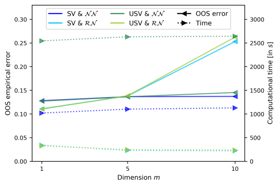
(a) Learning performance and computational time

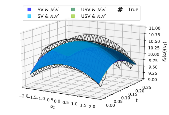
(b) Approximation for $m=1$

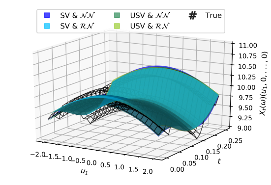
(c) Approximation for $m=5$

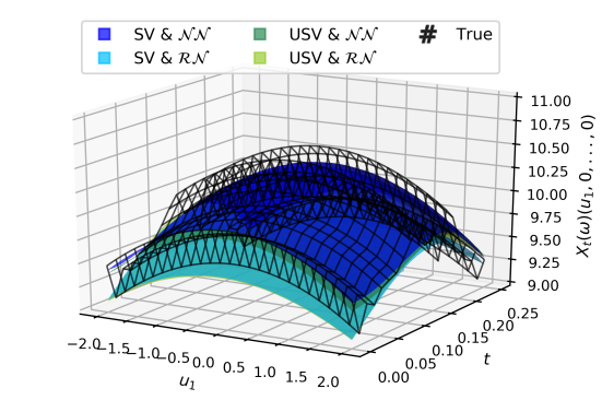
(d) Approximation for $m=10$

Figure 1. Learning the solution $X:[0,T]\times\Omega\rightarrow H$ of the stochastic heat equation (17) with neural networks (label “$\mathcal{NN}$”) and random neural networks (label “$\mathcal{RN}$”) in the chaos expansion, either via supervised learning (Algorithm 1; label “SV”) or unsupervised learning (Algorithm 2; label “USV”). In (1), the learning performance is displayed in terms of the out-of-sample (OOS) empirical error (15) together with the computational time. In (1)-(1), the learned solutions $[0,T]\times\mathbb{R}\ni(t,u_{1})\mapsto X^{(I,J,K)}_{t}(\omega)(u_{1},0,...,0)\in\mathbb{R}$, with $(I,J,K)=(1,5,1)$, are compared to the true solution $[0,T]\times\mathbb{R}\ni(t,u_{1})\mapsto X_{t}(\omega)(u_{1},0,...,0)\in\mathbb{R}$ obtained via (19) for different $m\in\{1,5,10\}$ and some $\omega\in\Omega$ of the test set.

5.2. Heath-Jarrow-Morton (HJM) equation in interest rate theory

In the second example, we learn the solution of the Heath-Jarrow-Morton (HJM) equation. To this end, we assume that $(H,\langle\cdot,\cdot\rangle_{H})$ is a separable Hilbert space consisting of continuous curves $x:[0,\infty)\rightarrow\mathbb{R}$ such that for every $u\in[0,\infty)$ the evaluation map $H\ni x\mapsto x(u)\in\mathbb{R}$ is continuous. Moreover, we assume that (SPDE) takes the form

$$\begin{cases}dX_{t}&=\left(\frac{d}{du}X_{t}+F(t,\cdot,X_{t})\right)dt+B(t,\cdot,X_{t})dW_{t},\quad\quad t\in[0,\infty),\\ X_{0}&=\chi_{0}\in H,\end{cases}$$ (21)

where $\chi_{0}\in H$ is deterministic, where $\frac{d}{du}=:A:\operatorname*{dom}(\frac{d}{du})\subseteq H\rightarrow H$ is the generator of the $C_{0}$-semigroup $(S_{t})_{t\in[0,T]}$ defined by $H\ni x\mapsto S_{t}x:=x(\cdot+t)\in H$, and where $W:[0,T]\times\Omega\rightarrow Z$ is a $Q$-Brownian motion with values on a (possibly different) separable Hilbert space $(Z,\langle\cdot,\cdot\rangle_{Z})$, with $Q\in L_{1}(Z;Z)$ and RKHS $(Z_{0},\langle\cdot,\cdot\rangle_{Z_{0}})$. Moreover, the diffusion coefficient $B:[0,T]\times\Omega\times H\rightarrow L_{2}(Z_{0};H)$ is assumed to be $(\mathcal{P}_{T}\otimes\mathcal{B}(H))/\mathcal{B}(L_{2}(Z_{0};H))$-measurable, and the drift coefficient $F:[0,T]\times\Omega\times H\rightarrow H$ is given by the famous HJM no-arbitrage condition (see [13, Eq. 6.2]), i.e.

$$\vspace{-0.02cm}F(t,\omega,x):=\left(u\mapsto\sum_{i=1}^{\infty}B(t,\omega,x)(\widetilde{e}_{i})(u)\int_{0}^{u}B(t,\omega,x)(\widetilde{e}_{i})(v)dv+B(t,\omega,x)(\eta(t,\omega,x))(u)\right)\in H,$$ (22)

for $(t,\omega,x)\in[0,T]\times\Omega\times H$, where $(\widetilde{e}_{i})_{i\in\mathbb{N}}:=\left(Q^{1/2}e_{i}\right)_{i\in\mathbb{N}}$ is an orthonormal basis of $(Z_{0},\langle\cdot,\cdot\rangle_{Z_{0}})$, and $\eta:=(\eta_{t})_{t\in[0,T]}:[0,T]\times\Omega\times H\rightarrow Z_{0}$ is any $(\mathcal{P}_{T}\otimes\mathcal{B}(H))/\mathcal{B}(Z_{0})$-measurable map.

Remark 5.3.

The solution $X:=(X_{t})_{t\in[0,T]}$ of the HJM equation (21) describes the instantaneous forward rate. Indeed, let $r:=(r_{t})_{t\in[0,\infty)}:[0,\infty)\times\Omega\rightarrow\mathbb{R}$ be the spot interest rate. Then, for any $t\in[0,T]$ and $u\in[0,\infty)$, the price of a zero coupon bond with maturity date $u$ and nominal value $\$1$ is defined as $P_{t}(u):=\mathbb{E}\big{[}\exp\big{(}\!\!-\int_{t}^{t+u}r_{s}ds\big{)}\big{|}\mathcal{F}_{t}\big{]}$. Hence, if $B(t,\omega,X_{t})\eta(t,\omega,X_{t})=0\in H$ for $(dt\otimes d\mathbb{P})$-a.e. $(t,\omega)\in[0,T]\times\Omega$, the process $X:=(X_{t})_{t\in[0,T]}:[0,T]\times\Omega\rightarrow H$ defined as

$$X_{t}:=\left(u\mapsto-\frac{\partial}{\partial u}\log(P_{t}(u))\right),\quad\quad t\in[0,T],$$

expresses the instantaneous forward rate in the sense that for every $t\in[0,T]$ and $u\in[0,\infty)$ it holds that $P_{t}(u)=\exp\big{(}\!\!-\int_{t}^{t+u}X_{t}(v-t)dv\big{)}$. For more details, we refer to [13, Chapter 6].

For the numerical experiment, we let $[0,\infty)\ni u\mapsto w(u):=\exp(0.1u)\in[0,\infty)$ and consider the Hilbert space $(H,\langle\cdot,\cdot\rangle_{H})$ consisting of absolutely continuous curves $x:[0,\infty)\rightarrow\mathbb{R}$ satisfying $\int_{0}^{\infty}x^{\prime}(u)^{2}w(u)du<\infty$, equipped with the inner product $\langle x,y\rangle_{H}:=x(0)y(0)+\int_{0}^{\infty}x^{\prime}(u)y^{\prime}(u)w(u)du$, for $x,y\in H$ (see also [13, Section 6.3.3] and [22]). Moreover, we set $Z:=\mathbb{R}$ and consider a real-valued $Q$-Brownian motion $W:[0,T]\times\Omega\rightarrow\mathbb{R}$, with $Q:=\operatorname{id}_{\mathbb{R}}\in L_{1}(\mathbb{R};\mathbb{R})$, and therefore $\lambda_{1}:=1$ and $\lambda_{i}:=0$ for all $i\in\mathbb{N}\cap[2,\infty)$, cf. (2). In addition, we assume that the spot interest rate $r:=(r_{t})_{t\in[0,T]}:[0,T]\times\Omega\rightarrow\mathbb{R}$ follows a Vasiček model

$$\begin{cases}dr_{t}&=(\mu-\kappa r_{t})dt+\sigma dW_{t},\quad\quad t\in[0,T],\\ r_{0}&\in\mathbb{R},\end{cases}$$

where $r_{0}\in\mathbb{R}$ is deterministic, and where $\mu,\kappa\in\mathbb{R}$ as well as $\sigma>0$ are given parameters. Then, by [13, Equation 2.33] (see also [23, Section 5.4.1]), this corresponds to the HJM equation (21) with coefficients $[0,T]\times\Omega\times H\ni(t,\omega,x)\mapsto B(t,\omega,x):=\left(z\mapsto\sigma\exp(-\kappa\,\cdot)z\right)\in L_{2}(\mathbb{R};H)$ and $[0,T]\times\Omega\times H\ni(t,\omega,x)\mapsto F(t,\omega,x):=\frac{\sigma^{2}}{\kappa}\exp(-\kappa\,\cdot)\left(1-\exp(-\kappa\,\cdot)\right)\in H$ by (22), whose solution is given by

$$X_{t}=\left(u\mapsto-\frac{\partial}{\partial u}\log(P_{t}(u))\right)=\left(u\mapsto r_{t}e^{-\kappa u}+\frac{\mu}{\kappa}\left(1-e^{-\kappa u}\right)-\frac{\sigma^{2}}{2\kappa^{2}}\left(1-e^{-\kappa u}\right)^{2}\right).$$ (23)

Now, we choose $I=1$, $T=1$, $r_{0}=4$, $\mu=4$, $\kappa=0.9$, and $\sigma=0.5$, let $(\omega_{m_{1}})_{m_{1}=1,...,M_{1}}\subseteq\Omega$ with $M_{1}=200$, let $(t_{m_{2}})_{m_{2}=0,...,M_{2}}\subseteq[0,T]$ be an equidistant time grid with $M_{2}=20$, and let $u_{1}:=0$ and $(u_{m_{3}})_{m_{3}=2,...,M_{3}}\sim C_{u}\mathds{1}_{[0,3]}(u)\exp(0.1u)du$ be an i.i.d. sequence of random variables with $M_{3}=81$, where $C_{u}>0$ is a normalizing constant. After splitting the data into 80%/20% for training/testing along $(\omega_{m_{1}})_{m_{1}=1,...,M_{1}}$, we run the algorithm for both the supervised and unsupervised approach, and both with deterministic and random neural networks (using the activation function $\rho(s):=\tanh(s)$, and with $N=25$ and $N=75$ neurons, respectively), where we choose $\widetilde{c}_{\beta,m_{1},m_{2},m_{3}}:=\mathds{1}_{\{0\}\times\{0\}}(\beta,m_{3})+\mathds{1}_{\{1\}\times\{2,...,M_{3}\}}(\beta,m_{3})$ for $\beta\in\mathbb{N}^{1}_{0,1}=\{0,1\}$, $m_{1}=1,...,M_{1}$, $m_{2}=0,...,M_{2}$, and $m_{3}=1,...,M_{3}$. This means that the empirical error (15) becomes now

$$\left(\sum_{m_{1}=1}^{M_{1}}\sum_{m_{2}=0}^{M_{2}}\left(\left|\left(X_{t_{m_{2}}}-X^{(I,J,K)}_{t_{m_{2}}}\right)(\omega_{m_{1}})(0)\right|^{2}+\sum_{m_{3}=1}^{M_{3}}\left|\frac{d}{du}\left(X_{t_{m_{2}}}-X^{(I,J,K)}_{t_{m_{2}}}\right)(\omega_{m_{1}})(u_{m_{3}})\right|^{2}\right)\right)^{\frac{1}{2}}$$

and analogously for (16), which is a truncated empirical version of the norm of $(H,\langle\cdot,\cdot\rangle_{H})$. For the training of deterministic networks, we apply the Adam algorithm (see [50]) over $10^{5}$ epochs with learning rate $5\cdot 10^{-4}$ and batchsize $40$, while the random networks are learned with the least squares method.

Figure 2 shows that deterministic and random neural networks in the Wiener chaos expansion are able to learn the solution of the HJM equation (21) via both learning approaches described in Algorithm 1+2. Moreover, Figure 2 (2) shows that a Gaussian approximation ($K=1$) is sufficient (see Remark 2.12).

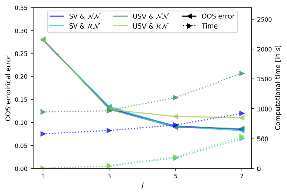
(a) Learning performance and computational time for $(J,K)\in\{1,3,5,7\}\times\{2\}$

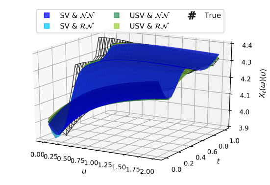
(b) Approximation for $(J,K)=(7,2)$

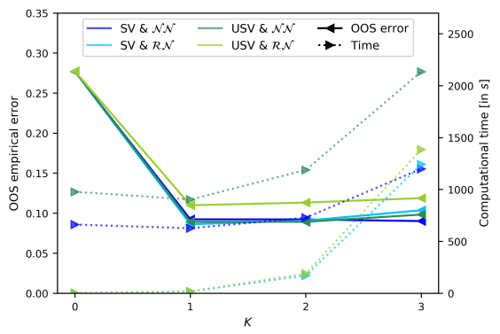
(c) Learning performance and computational time for $(J,K)\in\{5\}\times\{0,1,2,3\}$

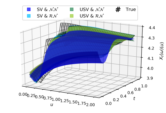
(d) Approximation for $(J,K)=(5,3)$

Figure 2. Learning the solution $X:[0,T]\times\Omega\rightarrow H$ of the HJM equation (21) with neural networks (label “$\mathcal{NN}$”) and random neural networks (label “$\mathcal{RN}$”) in the chaos expansion, either via supervised learning (Algorithm 1; label “SV”) or unsupervised learning (Algorithm 2; label “USV”). In (2)+(2), the learning performance is displayed in terms of the out-of-sample (OOS) empirical error (15) together with the computational time for different $J\in\{1,3,5,7\}$ and $K\in\{0,1,2,3\}$, respectively. In (2)+(2), the learned solutions $[0,T]\times\mathbb{R}\ni(t,u)\mapsto X^{(I,J,K)}_{t}(\omega)(u)\in\mathbb{R}$, with $(I,J,K)=(1,7,2)$ and $(I,J,K)=(1,5,3)$, are compared to the true solution $[0,T]\times\mathbb{R}\ni(t,u)\mapsto X_{t}(\omega)(u)\in\mathbb{R}$ obtained via (23) for some $\omega\in\Omega$ of the test set.

5.3. Zakai equation in filtering

In the third example, we consider the Zakai equation in filtering theory (see [47, 54, 88, 76]), which describes the evolution of an unnormalized density function of the conditional distribution of an unobservable process. To this end, we consider for some fixed $m\in\mathbb{N}$ the Hilbert space $(H,\langle\cdot,\cdot\rangle_{H}):=(L^{2}(\mathbb{R}^{m},\mathcal{L}(\mathbb{R}^{m}),w),\langle\cdot,\cdot\rangle_{L^{2}(\mathbb{R}^{m},\mathcal{L}(\mathbb{R}^{m}),w)})$, where $\mathbb{R}^{m}\ni u\mapsto w(u):=(2\pi)^{-m/2}\exp\left(-\|u\|^{2}/2\right)\in[0,\infty)$. Moreover, for $T>0$, we assume that $Y:=(Y_{t})_{t\in[0,T]}:[0,T]\times\Omega\rightarrow\mathbb{R}^{m}$ is an unobserved signal process satisfying

$$Y_{t}=Y_{0}+\int_{0}^{t}\mu(Y_{s})ds+\int_{0}^{t}\sigma(Y_{s})d\widetilde{W}_{s},\quad\quad t\in[0,T],$$ (24)

where $Y_{0}$ is $\mathcal{F}_{0}$-measurable with probability density function $\chi_{0}:\mathbb{R}^{m}\rightarrow[0,\infty)$, where $\mu\in C^{2}_{b}(\mathbb{R}^{m};\mathbb{R}^{m})$ and $\sigma\in C^{3}_{b}(\mathbb{R}^{m};\mathbb{R}^{m\times m})$ are the SDE-coefficients, and where $\widetilde{W}:=(\widetilde{W}_{t})_{t\in[0,T]}:[0,T]\times\Omega\rightarrow\mathbb{R}^{m}$ is an $m$-dimensional Brownian motion. Then, $Y:[0,T]\times\Omega\rightarrow\mathbb{R}^{m}$ is a Markov process with generator

$$C^{\infty}_{c}(\mathbb{R}^{m})\ni x\quad\mapsto\quad\mathcal{A}x:=\frac{1}{2}\operatorname*{tr}\left(\sigma(\cdot)\sigma(\cdot)^{\top}\nabla^{2}x(\cdot)\right)+\mu(\cdot)^{\top}\nabla x(\cdot)\in C^{\infty}_{c}(\mathbb{R}^{m})\subseteq L^{2}(\mathbb{R}^{m},\mathcal{L}(\mathbb{R}^{m}),w),$$ (25)

where $\nabla x(u):=\big{(}\frac{\partial x}{\partial u_{i}}(u)\big{)}_{i=1,...,m}\in\mathbb{R}^{m}$ and $\nabla^{2}x(u):=\big{(}\frac{\partial^{2}x}{\partial u_{i}\partial u_{j}}(u)\big{)}_{i,j=1,...,m}\in\mathbb{R}^{m\times m}$. Moreover, we assume that $Z:=(Z_{t})_{t\in[0,T]}:[0,T]\times\Omega\rightarrow\mathbb{R}^{n}$ is the observed process, which satisfies

$$Z_{t}=\int_{0}^{t}\kappa(Y_{s})ds+W_{t},\quad\quad t\in[0,T],$$ (26)

where $\kappa:\mathbb{R}^{m}\rightarrow\mathbb{R}^{n}$ is a continuous function, and where $\widetilde{W}:=(\widetilde{W}_{t})_{t\in[0,T]}:[0,T]\times\Omega\rightarrow\mathbb{R}^{n}$ is an $n$-dimensional Brownian motion, independent from $\widetilde{W}:[0,T]\times\Omega\rightarrow\mathbb{R}^{m}$. Then, by assuming that $\chi_{0}\in W^{2,2}(\mathbb{R}^{m},\mathcal{L}(\mathbb{R}^{m}),w)$, we can apply [76, Theorem 6.3] to conclude that the solution of the SPDE

$$\begin{cases}dX_{t}&=\left(\mathcal{A}^{*}X_{t}+F(t,\cdot,X_{t})\right)dt+B(t,\cdot,X_{t})dW_{t},\quad\quad t\in[0,T],\\ X_{0}&=\chi_{0}\in L^{2}(\mathbb{R}^{m},\mathcal{L}(\mathbb{R}^{d}),w),\end{cases}$$ (27)

describes at each time $t\in[0,T]$ an unnormalized density function of the conditional distribution of $Y_{t}$ given the observations of $(Z_{s})_{s\in[0,t]}$, which means that

$$\mathbb{P}\left[Y_{t}\in A\big{|}(Z_{s})_{s\in[0,t]}\right]=\frac{\int_{A}X_{t}(u)du}{\int_{\mathbb{R}^{m}}X_{t}(u)du},\quad\quad A\in\mathcal{L}(\mathbb{R}^{m}),$$

where $\mathcal{A}^{*}:\operatorname*{dom}(\mathcal{A}^{*}):=C^{\infty}_{c}(\mathbb{R}^{m})\subseteq L^{2}(\mathbb{R}^{m},\mathcal{L}(\mathbb{R}^{m}),w)\rightarrow L^{2}(\mathbb{R}^{m},\mathcal{L}(\mathbb{R}^{m}),w)$ is the adjoint of $\mathcal{A}$ given in (25), and where $W:=(W_{t})_{t\in[0,T]}:[0,T]\times\Omega\rightarrow Z:=\mathbb{R}^{m}$ is the $m$-dimensional Brownian motion from (26). Note that (27) is of the form (SPDE) with coefficients $F$ and $B$ given by

$$\times\Omega\times H\ni(t,\omega,x)\quad\mapsto\quad F(t,\omega,x) :=x(\cdot)\kappa(\cdot)^{\top}\kappa(Y_{t}(\omega))\in H$$

$$[0,T]\times\Omega\times H\ni(t,\omega,x)\quad\mapsto\quad B(t,\omega,x) :=\left(v\mapsto x(\cdot)\kappa(\cdot)^{\top}v\right)\in L_{2}(\mathbb{R}^{n};H),$$

where $H:=L^{2}(\mathbb{R}^{m},\mathcal{L}(\mathbb{R}^{m}),w)$. Since $X:=(X_{t})_{t\in[0,T]}$ depends on the randomness of both Brownian motions $W$ and $\widetilde{W}$ (the latter via $Y$ in $F$ and $B$), we have to include both of them into the computation of the Wick polynomials $(\xi_{\alpha})_{\alpha\in\mathcal{J}}$. This means that we consider the ($\mathbb{R}^{n}\times\mathbb{R}^{m}$)-valued $Q$-Brownian motion $\overline{W}:=(W_{t},\widetilde{W}_{t})_{t\in[0,T]}:[0,T]\times\Omega\rightarrow\mathbb{R}^{n}\times\mathbb{R}^{m}$, with $Q:=\operatorname{id}_{\mathbb{R}^{n}\times\mathbb{R}^{m}}\in L_{1}(\mathbb{R}^{n}\times\mathbb{R}^{m};\mathbb{R}^{n}\times\mathbb{R}^{m})$, and thus $\lambda_{i}:=1$ for all $i=1,...,m+n$, and $\lambda_{i}:=0$ for all $i\in\mathbb{N}\cap[m+n+1,\infty)$, cf. (2).

For the numerical example, we choose $m=2$ and $T=0.5$, the drift function $\mathbb{R}^{m}\ni y\mapsto\mu(y):=0.25\frac{y}{1+\|y\|^{2}}\in\mathbb{R}^{m}$, and diffusion function $\mathbb{R}^{m}\ni y\mapsto\sigma(y):=m^{-1/2}\mathbf{1}\in\mathbb{R}^{m\times m}$, with $\mathbf{1}\in\mathbb{R}^{m\times m}$ denoting the matrix having all entries equal to one, and assume that $Y_{0}\sim\mathcal{N}_{m}(0,I_{m})$, i.e. $\mathbb{R}^{m}\ni u\mapsto\chi_{0}(u):=\left(2\pi\right)^{-m/2}\exp\left(-\|u\|^{2}/2\right)\in\mathbb{R}$. Moreover, we consider $m=n$ and $\mathbb{R}^{m}\ni y\mapsto\kappa(y):=0.5y\in\mathbb{R}^{n}$. In addition, let $(\omega_{m_{1}})_{m_{1}=1,...,M_{1}}\subseteq\Omega$ with $M_{1}=300$, let $(t_{m_{2}})_{m_{2}=0,...,M_{2}}\subseteq[0,T]$ be an equidistant grid with $M_{2}=20$, and let $(u_{m_{3}})_{m_{3}=1,...,M_{3}}\sim\mathcal{N}_{m}(0,I_{m})$ be an i.i.d. sequence of normally distributed random variables with $M_{3}=150$. After splitting the data into 80%/20% for training/testing along $(\omega_{m_{1}})_{m_{1}=1,...,M_{1}}$, we run the algorithm for both the supervised and unsupervised approach, and both with deterministic and random neural networks (using the activation function $\rho(s):=\tanh(s)$, and with $N=25$ and $N=75$ neurons, respectively). For the training of deterministic networks, we apply the Adam algorithm (see [50]) over $10^{5}$ epochs with learning rate $5\cdot 10^{-4}$ and batchsize $40$, while the random networks are learned with the least squares method.

Figure 3 shows that the truncated Wiener chaos expansion with deterministic and random neural networks can learn the solution of the Zakai equation (27) using both Algorithm 1+2. Hereby, the true solution $X:[0,T]\times\Omega\rightarrow H$ of (27) is approximated with the Monte-Carlo method in [6].

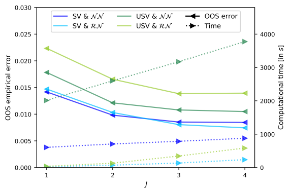
(a) Learning performance and computational time

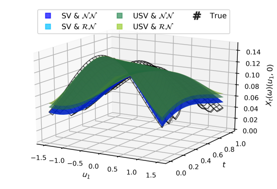
(b) Approximation for $J=5$

Figure 3. Learning the solution $X:[0,T]\times\Omega\rightarrow H$ of the Zakai equation (27) with neural networks (label “$\mathcal{NN}$”) and random neural networks (label “$\mathcal{RN}$”) in the chaos expansion, either via supervised learning (Algorithm 1; label “SV”) or unsupervised learning (Algorithm 2; label “USV”). In (3), the learning performance is displayed in terms of the out-of-sample (OOS) empirical error (15) together with the computational time for different $J\in\{1,...,5\}$. In (3), the learned solutions $[0,T]\times\mathbb{R}\ni(t,u_{1})\mapsto X^{(I,J,K)}_{t}(\omega)(u_{1},0)\in\mathbb{R}$, with $(I,J,K)=(2m,5,1)$, are compared to the true solution $[0,T]\times\mathbb{R}\ni(t,u_{1})\mapsto X_{t}(\omega)(u_{1},0)\in\mathbb{R}$ obtained via the Monte-Carlo method in [6] for some $\omega\in\Omega$ of the test set.

5.4. Conclusion

Figure 1-3 empirically demonstrate that deterministic and random neural networks in the truncated Wiener chaos are able to learn the solution of (SPDE). In the supervised learning approach (see Algorithm 1), the solution of (SPDE) is provided as a target, whereas the unsupervised learning approach (see Algorithm 2) recovers the solution by minimizing the (squared) difference of the left- and right-hand side of (SPDE). The latter is naturally more challenging and results in a higher out-of-sample error. Moreover, random neural networks have a slightly lower approximation accuracy than deterministic neural networks but are computationally more efficient (see also [66, Section 6] for a comparison).

6. Proofs

6.1. Proof of auxiliary results in Section 2

Proof of Proposition 2.5.

For any $p\in[1,\infty)$, we first apply [17, Theorem 7.2 (i)] to conclude that $X:[0,T]\times\Omega\rightarrow H$ exists, is unique up to modifications among the $\mathbb{F}$-predictable processes $\widetilde{X}:[0,T]\times\Omega\rightarrow H$ satisfying $\mathbb{P}\big{[}\int_{0}^{T}\|\widetilde{X}_{t}\|_{H}^{2}dt<\infty\big{]}=1$, and admits a continuous modification.

Now, for $p\in(2,\infty)$, we use [17, Theorem 7.2 (iii)] (with constant $\widetilde{C}^{(p)}_{F,B,S,T}>0$ depending only on $p\in(2,\infty)$, $C_{F,B}>0$, $C_{S}:=\sup_{t\in[0,T]}\|S_{t}\|_{L(H;H)}<\infty$, and $T>0$) and that the initial condition $\chi_{0}\in H$ is deterministic (see Assumption 2.3 (v)) implying that $X_{0}\in L^{p}(\Omega,\mathcal{F},\mathbb{P};H)$ to obtain that

$$\mathbb{E}\left[\sup_{t\in[0,T]}\|X_{t}\|_{H}^{p}\right] \leq\widetilde{C}^{(p)}_{F,B,S,T}\left(1+\mathbb{E}\left[\|X_{0}\|_{H}^{p}\right]\right)$$

$$=\widetilde{C}^{(p)}_{F,B,S,T}\left(1+\|\chi_{0}\|_{H}^{p}\right).$$

On the other hand, for $p\in[1,2]$, we use Jensen’s inequality, [17, Theorem 7.2 (iii)] (with exponent $3$ and constant $C^{(3)}_{F,B,S,T}>0$ depending only on $C_{F,B}>0$, $C_{S}:=\sup_{t\in[0,T]}\|S_{t}\|_{L(H;H)}<\infty$, and $T>0$), that the initial condition $\chi_{0}\in H$ is deterministic (see Assumption 2.3 (v)) implying that $X_{0}\in L^{3}(\Omega,\mathcal{F},\mathbb{P};H)$, and the inequality $(x+y)^{p/3}\leq\left(x^{p/3}+y^{p/3}\right)$ for any $x,y\geq 0$ to conclude that

$$\mathbb{E}\left[\sup_{t\in[0,T]}\|X_{t}\|_{H}^{p}\right] \leq\mathbb{E}\left[\sup_{t\in[0,T]}\|X_{t}\|_{H}^{3}\right]^{\frac{p}{3}}$$ (28)

$$\leq\left(\widetilde{C}^{(3)}_{F,B,S,T}\left(1+\mathbb{E}\left[\|X_{0}\|_{H}^{3}\right]\right)\right)^{\frac{p}{3}}$$

$$=\left(\widetilde{C}^{(3)}_{F,B,S,T}\right)^{\frac{p}{3}}\left(1+\|\chi_{0}\|_{H}^{3}\right)^{\frac{p}{3}}$$

$$\leq\left(\widetilde{C}^{(3)}_{F,B,S,T}\right)^{\frac{p}{3}}\left(1+\|\chi_{0}\|_{H}^{p}\right).$$

Hence, defining the constant $C^{(p)}_{F,B,S,T}>0$ by $C^{(p)}_{F,B,S,T}:=\widetilde{C}^{(p)}_{F,B,S,T}$ if $p\in(2,\infty)$, and by $C^{(p)}_{F,B,S,T}:=\big{(}\widetilde{C}^{(3)}_{F,B,S,T}\big{)}^{p/3}$ if $p\in[1,2]$, we obtain the result. ∎

Lemma 6.1.

Let $(H,\langle\cdot,\cdot\rangle_{H})$ be separable. Then, $(C^{0}([0,T];H),\|\cdot\|_{C^{0}([0,T];H)})$ is separable.

Proof.

By using that $(H,\langle\cdot,\cdot\rangle_{H})$ is separable, there exists a sequence $(x_{n})_{n\in\mathbb{N}}\subseteq H$ that is dense in $H$. From this, we define the countable set

$$\textup{Pol}_{\mathbb{Q}}([0,T];H):=\left\{[0,T]\ni t\mapsto\sum_{n=1}^{N}q_{n}(t)x_{n}\in H:\,\begin{matrix}N\in\mathbb{N},\,q_{1},...,q_{N}\in\textup{Pol}_{\mathbb{Q}}([0,T])\\ x_{1},...,x_{N}\in H\end{matrix}\right\},$$

where $\textup{Pol}_{\mathbb{Q}}([0,T]):=\big{\{}[0,T]\ni t\mapsto\sum_{k=0}^{K}c_{k}t^{k}\in\mathbb{R}:K\in\mathbb{N},\,c_{0},...,c_{K}\in\mathbb{Q}\big{\}}$. Then, $\textup{Pol}_{\mathbb{Q}}([0,T];H)$ is a $\textup{Pol}_{\mathbb{Q}}([0,T])$-submodule (i.e. for every $q\in\textup{Pol}_{\mathbb{Q}}([0,T])$ and $w\in\textup{Pol}_{\mathbb{Q}}([0,T];H)$ it holds that $q\cdot w\in\textup{Pol}_{\mathbb{Q}}([0,T];H)$). Moreover, $\textup{Pol}_{\mathbb{Q}}([0,T])$ is a subalgebra (i.e. for every $q_{1},q_{2}\in\textup{Pol}_{\mathbb{Q}}([0,T])$ it holds that $q_{1}+q_{2}\in\textup{Pol}_{\mathbb{Q}}([0,T])$ and $q_{1}\cdot q_{2}\in\textup{Pol}_{\mathbb{Q}}([0,T])$) which is point separating (i.e. for every distinct $t_{1},t_{2}\in[0,T]$ there exists some $q\in\textup{Pol}_{\mathbb{Q}}([0,T])$ with $q(t_{1})\neq q(t_{2})$) and nowhere vanishing (i.e. for every $t_{0}\in[0,T]$ there exists some $q\in\textup{Pol}_{\mathbb{Q}}([0,T])$ with $q(t_{0})\neq 0$). In addition, for every $t\in[0,T]$, the set $\{w(t):w\in\textup{Pol}_{\mathbb{Q}}([0,T];H)\}\supseteq\{x_{n}:n\in\mathbb{N}\}$ is dense in $H$. Then, we can apply the vector-valued Stone-Weierstrass theorem in [11, p. 103] to conclude that $\textup{Pol}_{\mathbb{Q}}([0,T];H)$ is dense in $C^{0}([0,T];H)$. Since $\textup{Pol}_{\mathbb{Q}}([0,T];H)$ is countable, $(C^{0}([0,T];H),\|\cdot\|_{C^{0}([0,T];H)})$ is separable. ∎

Proof of Lemma 2.6.

For (i), we fix some $j\in\mathbb{N}$ and $t\in[0,T]$. Then, by using the definition of $\xi_{i,j}$ in (6), that $\int_{0}^{t}g_{j}(s)ds=\langle\mathds{1}_{[0,t]},g_{j}\rangle_{L^{2}([0,T],\mathcal{B}([0,T]),dt)}$, Ito’s isometry, and that $(g_{j})_{i\in\mathbb{N}}$ is a complete orthonormal basis of $(L^{2}([0,T],\mathcal{B}([0,T]),dt),\langle\cdot,\cdot\rangle_{L^{2}([0,T],\mathcal{B}([0,T]),dt)})$, it follows that

$$\left\|W^{(i)}_{t}-\sum_{j=1}^{J}\xi_{i,j}\int_{0}^{t}g_{j}(s)ds\right\|_{L^{2}(\Omega,\mathcal{F},\mathbb{P})}$$

$$\quad\quad=\mathbb{E}\left[\left|W^{(i)}_{t}-\sum_{j=1}^{J}\xi_{i,j}\int_{0}^{t}g_{j}(s)ds\right|^{2}\right]^{\frac{1}{2}}$$

$$\quad\quad=\mathbb{E}\left[\left|\int_{0}^{T}\mathds{1}_{[0,t]}(s)dW^{(i)}_{s}-\sum_{j=1}^{J}\left(\int_{0}^{T}g_{j}(s)dW^{(i)}_{s}\right)\langle\mathds{1}_{[0,t]},g_{j}\rangle_{L^{2}([0,T],\mathcal{B}([0,T]),dt)}\right|^{2}\right]^{\frac{1}{2}}$$

$$\quad\quad=\mathbb{E}\left[\left|\int_{0}^{T}\left(\mathds{1}_{[0,t]}(s)-\sum_{j=1}^{J}\langle\mathds{1}_{[0,t]},g_{j}\rangle_{L^{2}([0,T],\mathcal{B}([0,T]),dt)}g_{j}(s)\right)dW^{(i)}_{s}\right|^{2}\right]^{\frac{1}{2}}$$

$$\quad\quad=\left(\int_{0}^{T}\left(\mathds{1}_{[0,t]}(s)-\sum_{j=1}^{J}\langle\mathds{1}_{[0,t]},g_{j}\rangle_{L^{2}([0,T],\mathcal{B}([0,T]),dt)}g_{j}(s)\right)^{2}ds\right)^{\frac{1}{2}}$$

$$\quad\quad=\left\|\mathds{1}_{[0,t]}-\sum_{j=1}^{J}\langle\mathds{1}_{[0,t]},g_{j}\rangle_{L^{2}([0,T],\mathcal{B}([0,T]),dt)}g_{j}\right\|_{L^{2}([0,T],\mathcal{B}([0,T]),dt)}\quad\overset{J\rightarrow\infty}{\longrightarrow}\quad 0.$$

For (ii), we use Minkowski’s inequality, that $(e_{i})_{i\in\mathbb{N}}$ is an orthonormal basis of $(Z,\langle\cdot,\cdot\rangle_{Z})$, that $\sum_{i=1}^{\infty}\lambda_{i}<\infty$, that $W^{(i)}_{t}-\sum_{j=1}^{J}\xi_{i,j}\int_{0}^{t}g_{j}(s)ds\sim W^{(1)}_{t}-\sum_{j=1}^{J}\xi_{1,j}\int_{0}^{t}g_{j}(s)ds$ are identically distributed for any $i\in\mathbb{N}$, Lemma 2.2, and (i) to conclude that

$$\left\|W_{t}-\sum_{i=1}^{I}\sum_{j=1}^{J}\sqrt{\lambda_{i}}\xi_{i,j}\left(\int_{0}^{t}g_{j}(s)ds\right)e_{i}\right\|_{L^{2}(\Omega,\mathcal{F},\mathbb{P};Z)}$$

$$\quad\quad=\mathbb{E}\left[\left\|W_{t}-\sum_{i=1}^{I}\sum_{j=1}^{J}\sqrt{\lambda_{i}}\xi_{i,j}\left(\int_{0}^{t}g_{j}(s)ds\right)e_{i}\right\|_{Z}^{2}\right]^{\frac{1}{2}}$$

$$\quad\quad\leq\mathbb{E}\left[\left\|W_{t}-\sum_{i=1}^{I}\sqrt{\lambda_{i}}W^{(i)}_{t}e_{i}\right\|_{Z}^{2}\right]^{\frac{1}{2}}+\mathbb{E}\left[\left\|\sum_{i=1}^{I}\sqrt{\lambda_{i}}W^{(i)}_{t}e_{i}-\sum_{i=1}^{I}\sum_{j=1}^{J}\sqrt{\lambda_{i}}\xi_{i,j}\left(\int_{0}^{t}g_{j}(s)ds\right)e_{i}\right\|_{Z}^{2}\right]^{\frac{1}{2}}$$

$$\quad\quad=\mathbb{E}\left[\left\|W_{t}-\sum_{i=1}^{I}\sqrt{\lambda_{i}}W^{(i)}_{t}e_{i}\right\|_{Z}^{2}\right]^{\frac{1}{2}}+\sum_{i=1}^{I}\lambda_{i}\mathbb{E}\left[\left|W^{(i)}_{t}-\sum_{j=1}^{J}\xi_{i,j}\int_{0}^{t}g_{j}(s)ds\right|^{2}\right]^{\frac{1}{2}}$$

$$\quad\quad\leq\mathbb{E}\left[\left\|W_{t}-\sum_{i=1}^{I}\sqrt{\lambda_{i}}W^{(i)}_{t}e_{i}\right\|_{Z}^{2}\right]^{\frac{1}{2}}+\left(\sum_{i=1}^{\infty}\lambda_{i}\right)\mathbb{E}\left[\left|W^{(1)}_{t}-\sum_{j=1}^{J}\xi_{1,j}\int_{0}^{t}g_{j}(s)ds\right|^{2}\right]^{\frac{1}{2}}$$

$$\quad\quad\quad\overset{I,J\rightarrow\infty}{\longrightarrow}\quad 0,$$

which completes the proof. ∎

Proof of Lemma 2.10.

Fix some $p\in[1,\infty)$. Moreover, we define the map

$$L^{2}([0,T];L_{2}(Z_{0};\mathbb{R}))\ni\psi\quad\mapsto\quad\mathscr{W}(\psi):=\int_{0}^{T}\psi(t)dW_{t}\in L^{2}(\Omega,\mathcal{F}_{T},\mathbb{P})$$

returning the stochastic integral of a deterministic function $\psi:[0,T]\rightarrow L_{2}(Z_{0};\mathbb{R})$ at terminal time $T>0$. Then, by using Ito’s isometry in [17, Proposition 4.28] (with $\operatorname*{tr}\big{(}\big{(}\Xi_{1}Q^{1/2}\big{)}\big{(}\Xi_{2}Q^{1/2}\big{)}^{*}\big{)}=\langle\Xi_{1},\Xi_{2}\rangle_{L_{2}(Z_{0};H)}$ for any $\Xi_{1},\Xi_{2}\in L_{2}(Z_{0};H)$, see [17, Appendix C]), it follows for every $\psi,\phi\in L^{2}([0,T];L_{2}(Z_{0};\mathbb{R}))$ that

$$\mathbb{E}[\mathscr{W}(\psi)]=\mathbb{E}\left[\int_{0}^{T}\psi(t)dW_{t}\right]=0$$

and that

$$\mathbb{E}[\mathscr{W}(\psi)\mathscr{W}(\phi)] =\mathbb{E}\left[\left(\int_{0}^{T}\psi(t)dW_{t}\right)\left(\int_{0}^{T}\phi(t)dW_{t}\right)\right]$$

$$=\mathbb{E}\left[\int_{0}^{T}\langle\psi(t),\phi(t)\rangle_{L_{2}(Z_{0};\mathbb{R})}dt\right]$$

$$=\langle\psi,\phi\rangle_{L^{2}([0,T];L_{2}(Z_{0};\mathbb{R}))},$$

which shows that $\mathscr{W}$ is an isonormal process in the sense of [70, Definition 1.1.1]. Hence, by using [70, Exercise 1.1.7] (see also [69, Theorem 2.2.4 (i)]), we conclude that

$$\left\{q\left(\mathscr{W}(\psi_{1}),...,\mathscr{W}(\psi_{n})\right):n\in\mathbb{N},\,q\in\textup{Pol}(\mathbb{R}^{n}),\,\psi_{1},...,\psi_{n}\in L^{2}([0,T];L_{2}(Z_{0};\mathbb{R}))\right\}$$ (29)

is dense in $L^{p}(\Omega,\mathcal{F}_{T},\mathbb{P})$, where $\textup{Pol}(\mathbb{R}^{n})$ consists of polynomials of the form $\mathbb{R}^{n}\ni x:=(x_{1},...,x_{n})^{\top}\mapsto\sum_{\mathbf{k}\in\mathbb{N}^{n}_{0,K}}a_{\mathbf{k}}\prod_{l=1}^{n}x_{l}^{k_{l}}\in\mathbb{R}$ for some $N\in\mathbb{N}$ and $(a_{\mathbf{k}})_{\mathbf{k}\in\mathbb{N}^{n}_{0,K}}\subseteq\mathbb{R}$, where $\mathbf{k}:=(k_{1},...,k_{n})\in\mathbb{N}^{n}_{0,K}$.

Now, we show that $\operatorname*{span}\{\xi_{\alpha}:\alpha\in\mathcal{J}\}$ is also dense in $L^{p}(\Omega,\mathcal{F}_{T},\mathbb{P})$. Let us define for every $i,j\in\mathbb{N}$ the deterministic function $\big{(}t\mapsto\phi_{i,j}(t):=\left(z\mapsto g_{j}(t)\langle\widetilde{e}_{i},z\rangle_{Z_{0}}\right)\big{)}\in L^{2}([0,T];L_{2}(Z_{0};\mathbb{R}))$ satisfying $\xi_{i,j}=\int_{0}^{T}g_{j}(t)dW^{(i)}_{t}=\lambda_{i}^{-1/2}\int_{0}^{T}g_{j}(t)\langle e_{i},dW_{t}\rangle_{Z}=\int_{0}^{T}\phi_{i,j}(t)dW_{t}$, where $(\widetilde{e}_{i})_{i\in\mathbb{N}}:=\big{(}Q^{1/2}e_{i}\big{)}_{i\in\mathbb{N}}$ is an orthonormal basis of $(Z_{0},\langle\cdot,\cdot\rangle_{Z_{0}})$. Since $\xi_{\alpha}=\frac{1}{\sqrt{\alpha!}}\prod_{i,j=1}^{\infty}h_{\alpha_{i,j}}(\xi_{i,j})=\frac{1}{\sqrt{\alpha!}}\prod_{i,j=1}^{\infty}h_{\alpha_{i,j}}(\mathscr{W}(\phi_{i,j}))$ for any $\alpha\in\mathcal{J}$ and $\operatorname*{span}\left\{\mathbb{R}^{n}\ni(s_{1},...,s_{n})\mapsto\prod_{i=1}^{n}h_{k_{i}}(s_{i})\in\mathbb{R}:k_{1},...,k_{n}\in\mathbb{N}_{0}\right\}=\textup{Pol}(\mathbb{R}^{n})$ for any $n\in\mathbb{N}$, it therefore suffices to show that

$$\left\{q\left(\mathscr{W}(\phi_{i_{1},j_{1}}),...,\mathscr{W}(\phi_{i_{n},j_{n}})\right):n\in\mathbb{N},\,q\in\textup{Pol}(\mathbb{R}^{n}),\,(i_{1},j_{1}),...,(i_{n},j_{n})\in\mathbb{N}^{2}\right\}$$ (30)

is dense in $L^{p}(\Omega,\mathcal{F}_{T},\mathbb{P})$. To this end, we fix some $Z\in L^{p}(\Omega,\mathcal{F}_{T},\mathbb{P})$ and $\varepsilon\in(0,1)$. Then, by using that (29) is dense in $L^{p}(\Omega,\mathcal{F}_{T},\mathbb{P})$ there exists some $n\in\mathbb{N}$, $q\in\textup{Pol}(\mathbb{R}^{n})$, and $\psi_{1},...,\psi_{n}\in L^{2}([0,T];L_{2}(Z_{0};\mathbb{R}))$ such that

$$\mathbb{E}\left[|Z-q\left(\mathscr{W}(\psi_{1}),...,\mathscr{W}(\psi_{n})\right)|^{p}\right]^{\frac{1}{p}}<\frac{\varepsilon}{2}.$$ (31)

Moreover, for every fixed $l=1,...,n$, we use that the system $(\phi_{i,j})_{i,j\in\mathbb{N}}$ forms an orthonormal basis of $(L^{2}([0,T];L_{2}(Z_{0};\mathbb{R})),\langle\cdot,\cdot\rangle_{L^{2}([0,T];L_{2}(Z_{0};\mathbb{R}))})$ to conclude that there exist some $I_{l}\in\mathbb{N}$ and $J_{l}\in\mathbb{N}$ such that $\phi_{l}:=\sum_{i=1}^{I_{l}}\sum_{j=1}^{J_{l}}c_{l,i,j}\phi_{i,j}\in\operatorname*{span}\left\{\phi_{i,j}:i,j\in\mathbb{N}\right\}$ (with $c_{l,i,j}:=\langle\psi_{l},\phi_{i,j}\rangle_{L^{2}([0,T];L_{2}(Z_{0};\mathbb{R}))}$) satisfies

$$\left\|\psi_{l}-\phi_{l}\right\|_{L^{2}([0,T];L_{2}(Z_{0};\mathbb{R}))}<(2C_{\psi})^{-1}C_{N(n+1)p}^{-\frac{1}{(n+1)p}}\varepsilon,$$ (32)

where $C_{\psi}:=1+\sum_{\beta\in\mathbb{N}^{n}_{0,N}}\mathbb{E}\left[\left|\partial_{\beta}q\left(\mathscr{W}(\psi_{1}),...,\mathscr{W}(\psi_{n})\right)\right|^{(n+1)p}\right]^{1/((n+1)p)}\geq 1$, and where $C_{N(n+1)p}>0$ is the constant in [17, Theorem 4.36] (with exponent $N(n+1)p\geq 2$). Hence, for every $k=1,...,N$, we use [17, Theorem 4.36] (with exponent $N(n+1)p\geq 2$ and constant $C_{k(n+1)p}\geq 1$, which is increasing in $k\in\mathbb{N}$), the inequality (32), that $2C_{\psi}\geq 1$, that $C_{k(n+1)p}\geq 1$, and that $\varepsilon\in(0,1)$ to conclude that

$$\mathbb{E}\left[\left|\mathscr{W}(\phi_{l}-\psi_{l})\right|^{k(n+1)p}\right]^{\frac{1}{(n+1)p}} =\mathbb{E}\left[\left|\int_{0}^{T}\left(\phi_{l}(t)-\psi_{l}(t)\right)dW_{t}\right|^{k(n+1)p}\right]^{\frac{1}{(n+1)p}}$$ (33)

$$\leq C_{k(n+1)p}^{\frac{1}{(n+1)p}}\left(\mathbb{E}\left[\int_{0}^{T}\|\phi_{l}(t)-\psi_{l}(t)\|_{L_{2}(Z_{0};\mathbb{R})}^{2}dt\right]\right)^{\frac{k}{2}}$$

$$\leq C_{N(n+1)p}^{\frac{1}{(n+1)p}}\left\|\psi_{l}-\phi_{l}\right\|_{L^{2}([0,T];L_{2}(Z_{0};\mathbb{R}))}^{k}$$

$$<C_{N(n+1)p}^{\frac{1}{(n+1)p}}\left((2C_{\psi})^{-1}C_{N(n+1)p}^{-\frac{1}{(n+1)p}}\varepsilon\right)^{k}$$

$$\leq(2C_{\psi})^{-1}\varepsilon.$$

Thus, by using Minkwoski’s inequality, the inequality (31), Taylor’s theorem, i.e. that $q(y)-q(x)=\sum_{\beta\in\mathbb{N}^{n}_{0,N},\,|\beta|\geq 1}\frac{\partial_{\beta}q(x)}{\beta!}\prod_{l=1}^{N}(y_{l}-x_{l})^{\beta_{l}}$ for any $x:=(x_{1},...,x_{n})^{\top},y:=(y_{1},...,y_{n})^{\top}\in\mathbb{R}^{n}$, together with Minkwoski’s inequality, the generalized Hölder’s inequality (with exponents $\frac{1}{(n+1)p}+\sum_{l=1}^{n}\frac{1}{(n+1)p}=\frac{1}{p}$), the inequality (33), that $2C_{\psi}\geq 1$, and that $\varepsilon\in(0,1)$, it follows for $q\left(\mathscr{W}(\phi_{1}),...,\mathscr{W}(\phi_{n})\right)$ belonging to (30) (as $\mathscr{W}(\phi_{l})=\sum_{i=1}^{I_{l}}\sum_{j=1}^{J_{l}}c_{l,i,j}\mathscr{W}(\phi_{i,j})$ for any $l=1,...,n$) that

$$\mathbb{E}\left[|Z-q\left(\mathscr{W}(\phi_{1}),...,\mathscr{W}(\phi_{n})\right)|^{p}\right]^{\frac{1}{p}}$$

$$\quad\quad\leq\mathbb{E}\left[|Z-q\left(\mathscr{W}(\psi_{1}),...,\mathscr{W}(\psi_{n})\right)|^{p}\right]^{\frac{1}{p}}+\mathbb{E}\left[|q\left(\mathscr{W}(\psi_{1}),...,\mathscr{W}(\psi_{n})\right)-q\left(\mathscr{W}(\phi_{1}),...,\mathscr{W}(\phi_{n})\right)|^{p}\right]^{\frac{1}{p}}$$

$$\quad\quad<\mathbb{E}\left[|Z-q\left(\mathscr{W}(\psi_{1}),...,\mathscr{W}(\psi_{n})\right)|^{p}\right]^{\frac{1}{p}}$$

$$\quad\quad\quad\quad+\sum_{\beta\in\mathbb{N}^{n}_{0,N}\atop|\beta|\geq 1}\mathbb{E}\left[\left|\frac{\partial_{\beta}q\left(\mathscr{W}(\psi_{1}),...,\mathscr{W}(\psi_{n})\right)}{\beta!}\prod_{l=1}^{n}(\mathscr{W}(\phi_{l})-\mathscr{W}(\psi_{l}))^{\beta_{l}}\right|^{p}\right]^{\frac{1}{p}}$$

$$\quad\quad<\mathbb{E}\left[|Z-q\left(\mathscr{W}(\psi_{1}),...,\mathscr{W}(\psi_{n})\right)|^{p}\right]^{\frac{1}{p}}$$

$$\quad\quad\quad\quad+\sum_{\beta\in\mathbb{N}^{n}_{0,N}\atop|\beta|\geq 1}\frac{1}{\beta!}\mathbb{E}\left[\left|\partial_{\beta}q\left(\mathscr{W}(\psi_{1}),...,\mathscr{W}(\psi_{n})\right)\right|^{(n+1)p}\right]^{\frac{1}{(n+1)p}}\prod_{l=1}^{n}\mathbb{E}\left[\left|\mathscr{W}(\phi_{l}-\psi_{l})\right|^{\beta_{l}(n+1)p}\right]^{\frac{1}{(n+1)p}}$$

$$\quad\quad<\mathbb{E}\left[|Z-q\left(\mathscr{W}(\psi_{1}),...,\mathscr{W}(\psi_{n})\right)|^{p}\right]^{\frac{1}{p}}+C_{\psi}\max_{\beta\in\mathbb{N}^{n}_{0,N}\atop|\beta|\geq 1}\prod_{l=1}^{n}\left((2C_{\psi})^{-1}\varepsilon\right)^{\beta_{l}}$$

$$\quad\quad\leq\frac{\varepsilon}{2}+C_{\psi}(2C_{\psi})^{-1}\varepsilon=\varepsilon.$$

Since $Z\in L^{p}(\Omega,\mathcal{F}_{T},\mathbb{P})$ and $\varepsilon>0$ were chosen arbitrarily, this shows that (30) is dense in $L^{p}(\Omega,\mathcal{F}_{T},\mathbb{P})$ and therefore that $\operatorname*{span}\{\xi_{\alpha}:\alpha\in\mathcal{J}\}$ is also dense in $L^{p}(\Omega,\mathcal{F}_{T},\mathbb{P})$. Finally, for $p=2$, the Wick polynomials $(\xi_{\alpha})_{\alpha\in\mathcal{J}}$ are by [70, Proposition 1.1.1] a complete orthonormal basis of $L^{2}(\Omega,\mathcal{F}_{T},\mathbb{P})$. ∎

6.2. Proof of Theorem 2.11

Proof of Theorem 2.11.

For (9), we fix some $\varepsilon>0$. Then, by using the continuous modification, Proposition 2.5, and that the Brownian motion $W:[0,T]\times\Omega\rightarrow Z$ is the only random force driving (SPDE), we observe that $X\in L^{p}(\Omega,\mathcal{F}_{T},\mathbb{P};C^{0}([0,T];H))$. Moreover, by combining [41, Lemma 1.2.19 (i)] with Lemma 2.10, the linear span of $\left\{\Omega\ni\omega\mapsto\xi_{\alpha}(\omega)z\in C^{0}([0,T];H):\alpha\in\mathcal{J},\,z\in C^{0}([0,T];H)\right\}$ is dense in $L^{p}(\Omega,\mathcal{F}_{T},\mathbb{P};C^{0}([0,T];H))$. Hence, there exist some $I,J,K\in\mathbb{N}$ and $(x_{\alpha})_{\alpha\in\mathcal{J}_{I,J,K}}\subseteq C^{0}([0,T];H)$ such that

$$\mathbb{E}\left[\sup_{t\in[0,T]}\left\|X_{t}-\sum_{\alpha\in\mathcal{J}_{I,J,K}}x_{\alpha}(t)\xi_{\alpha}\right\|^{p}\right]^{\frac{1}{p}}=\mathbb{E}\left[\left\|X-\sum_{\alpha\in\mathcal{J}_{I,J,K}}x_{\alpha}\xi_{\alpha}\right\|_{C^{0}([0,T];H)}^{p}\right]^{\frac{1}{p}}<\varepsilon.$$

which shows the conclusion in (9).

For (10), we fix an orthonormal basis $(y_{n})_{n\in\mathbb{N}}$ of $(H,\langle\cdot,\cdot\rangle_{H})$. Then, we claim that $(\xi_{\alpha}y_{n})_{(\alpha,n)\in\mathcal{J}\times\mathbb{N}}$ is an orthonormal basis of the Bochner space $L^{2}(\Omega,\mathcal{F}_{T},\mathbb{P};H)$, where $\langle F,G\rangle_{L^{2}(\Omega,\mathcal{F},\mathbb{P};H)}:=\mathbb{E}[\langle F,G\rangle_{H}]$ is the inner product. Indeed, by using that $(\xi_{\alpha})_{\alpha\in\mathcal{J}}$ are by Lemma 2.10 orthonormal in $L^{2}(\Omega,\mathcal{F}_{T},\mathbb{P})$ and that $(y_{n})_{n\in\mathbb{N}}$ are by assumption orthonormal in $H$, it follows for every $\alpha,\beta\in\mathcal{J}$ and $l,m\in\mathbb{N}$ that

$$\langle\xi_{\alpha}y_{n},\xi_{\beta}y_{m}\rangle_{L^{2}(\Omega,\mathcal{F},\mathbb{P};H)}=\mathbb{E}\left[\langle\xi_{\alpha}y_{n},\xi_{\beta}y_{m}\rangle_{H}\right]=\mathbb{E}[\xi_{\alpha}\xi_{\beta}]\langle y_{n},y_{m}\rangle_{H}=\delta_{\alpha,\beta}\delta_{\beta,m}=\delta_{(\alpha,n),(\beta,m)}.$$

Moreover, by combining [41, Lemma 1.2.19 (i)] with Lemma 2.10, we conclude that the linear span of $\left\{\Omega\ni\omega\mapsto\xi_{\alpha}(\omega)y_{n}\in H:(\alpha,n)\in\mathcal{J}\times\mathbb{N}\right\}$ is dense in $L^{2}(\Omega,\mathcal{F}_{T},\mathbb{P};H)$. This shows that $(\xi_{\alpha}y_{n})_{(\alpha,n)\in\mathcal{J}\times\mathbb{N}}$ is an orthonormal basis of $L^{2}(\Omega,\mathcal{F}_{T},\mathbb{P};H)$. Hence, the chaos expansion (10) follows as an orthogonal expansion along the basis elements $(\xi_{\alpha}y_{n})_{(\alpha,n)\in\mathcal{J}\times\mathbb{N}}$ of $L^{2}(\Omega,\mathcal{F}_{T},\mathbb{P};H)$. ∎

6.3. Proof of auxiliary results in Section 3

Lemma 6.2.

Let $(H,\langle\cdot,\cdot\rangle_{H})$ satisfy Assumption 3.1. Then, the time-extended restriction map

$$(C^{k}_{b}(\mathbb{R}\times\mathbb{R}^{m};\mathbb{R}^{d}),\|\cdot\|_{C^{k}_{pol,\gamma}(\mathbb{R}\times\mathbb{R}^{m};\mathbb{R}^{d})})\ni f\,\,\mapsto\,\,\left(t\mapsto f(t,\cdot)|_{U}\right)\in(C^{0}([0,T];H),\|\cdot\|_{C^{0}([0,T];H)})$$ (34)

is a continuous dense embedding. Moreover, for every $\rho\in\overline{C^{k}_{b}(\mathbb{R})}^{\gamma}$ and $\varphi\in\mathcal{NN}^{\rho}_{[0,T]\times U,d}$, it holds that $(t\mapsto\varphi(t,\cdot))\in C^{0}([0,T];H)$.

Proof.

In order to show that (34) is a continuous embedding, we observe that for every $f\in C^{k}_{b}(\mathbb{R}\times\mathbb{R}^{m};\mathbb{R}^{d})$ it holds that

$$\|f\|_{C^{0}([0,T];H)} =\sup_{t\in[0,T]}\|f(t,\cdot)\|_{H}$$

$$\leq C_{H}\sup_{t\in[0,T]}\|f(t,\cdot)\|_{C^{k}_{pol,\gamma}(\mathbb{R}^{m};\mathbb{R}^{d})}$$

$$=C_{H}\sup_{t\in[0,T]}\max_{\beta\in\mathbb{N}^{m}_{0,k}}\sup_{u\in\mathbb{R}^{m}}\frac{\|\partial_{(0,\beta)}f(t,u)\|}{(1+\|u\|)^{\gamma}}$$

$$\leq C_{H}\max_{\beta\in\mathbb{N}^{m+1}_{0,k}}\sup_{(t,u)\in\mathbb{R}\times\mathbb{R}^{m}}\frac{\|\partial_{\beta}f(t,u)\|}{(1+\|(t,u)\|)^{\gamma}}$$

$$=C_{H}\|f\|_{C^{k}_{pol,\gamma}(\mathbb{R}\times\mathbb{R}^{m};\mathbb{R}^{d})}.$$

Next, for showing that (34) is a dense embedding, we fix some $f\in C^{0}([0,T];H)$ and $\varepsilon>0$. Moreover, we define the collection $(V_{t})_{t\in[0,T]}$ of open subsets $V_{t}:=\left\{s\in[0,T]:\|f(t,\cdot)-f(s,\cdot)\|_{H}<\varepsilon/2\right\}\subseteq[0,T]$ for $t\in[0,T]$, which forms an open cover of $[0,T]$. Then, by using that $[0,T]$ is compact, there exists some $N\in\mathbb{N}$ and $t_{1},...,t_{N}\in[0,T]$ such that $(V_{t_{n}})_{n=1,...,N}$ is a finite subcover of $[0,T]$. In addition, for every $n=1,...,N$, we use that the restriction map (11) is a dense embedding (see Assumption 3.1) to conclude that there exists some $g_{n}\in C^{k}_{b}(\mathbb{R}^{m};\mathbb{R}^{d})$ such that $\|f(t_{n},\cdot)-g_{n}|_{U}\|_{H}<\varepsilon/2$. Thus, by using a partition of unity $(\eta_{n})_{n=1,...,N}\subseteq C^{0}([0,T])$ subordinate to $(V_{t_{n}})_{n=1,...,N}$ (i.e. functions $(\eta_{n})_{n=1,...,N}\subseteq C^{0}([0,T])$ such that $0\leq\eta_{n}(t)\leq 1$ for all $t\in[0,T]$ and $n=1,...,N$, that $\sum_{n=1}^{N}\eta_{n}(t)=1$ for all $t\in[0,T]$, and that $\operatorname{supp}(\eta_{n}):=\overline{\{t\in[0,T]:\eta_{n}(t)\neq 0\}}\subseteq V_{t_{n}}$ for all $n=1,...,N$), we conclude for the function $\big{(}t\mapsto g(t):=\sum_{n=1}^{N}\eta_{n}(t)g_{n}\big{)}\in C^{0}([0,T];H)$ that

$$\|f-g|_{[0,T]\times U}\|_{C^{0}([0,T];H)}$$

$$\quad\quad=\sup_{t\in[0,T]}\left\|f(t,\cdot)-\sum_{n=1}^{N}\eta_{n}(t)g_{n}|_{U}\right\|_{H}$$

$$\quad\quad\leq\sup_{t\in[0,T]}\left\|f(t,\cdot)-\sum_{n=1}^{N}\eta_{n}(t)f(t_{n},\cdot)\right\|_{H}+\sup_{t\in[0,T]}\left\|\sum_{n=1}^{N}\eta_{n}(t)f(t_{n},\cdot)-\sum_{n=1}^{N}\eta_{n}(t)g_{n}|_{U}\right\|_{H}$$

$$\quad\quad\leq\sup_{t\in[0,T]}\left\|\sum_{n=1}^{N}\eta_{n}(t)(f(t,\cdot)-f(t_{n},\cdot))\right\|_{H}+\sup_{t\in[0,T]}\left\|\sum_{n=1}^{N}\eta_{n}(t)(f(t_{n},\cdot)-g_{n}|_{U})\right\|_{H}$$

$$\quad\quad\leq\sup_{t\in[0,T]}\sum_{n=1}^{N}\eta_{n}(t)\underbrace{\left\|f(t,\cdot)-f(t_{n},\cdot)\right\|_{H}}_{<\varepsilon/2}+\sup_{t\in[0,T]}\sum_{n=1}^{N}\eta_{n}(t)\underbrace{\left\|f(t_{n},\cdot)-g_{n}|_{U}\right\|_{H}}_{<\varepsilon/2}$$

$$\quad\quad<\frac{\varepsilon}{2}\sup_{t\in[0,T]}\sum_{n=1}^{N}\eta_{n}(t)+\frac{\varepsilon}{2}\sup_{t\in[0,T]}\sum_{n=1}^{N}\eta_{n}(t)$$

$$\quad\quad=\frac{\varepsilon}{2}+\frac{\varepsilon}{2}=\varepsilon.$$

Since $f\in C^{0}([0,T];H)$ and $\varepsilon>0$ were chosen arbitrarily, this shows that (34) is a dense embedding.

Finally, we use the previous step to conclude that $C^{0}([0,T];H)$ satisfies the conditions of [67, Definition 2.3]. Hence, by applying [67, Lemma 2.5], it follows for every $\rho\in\overline{C^{k}_{b}(\mathbb{R})}^{\gamma}$ and $\varphi\in\mathcal{NN}^{\rho}_{[0,T]\times U,d}$ that $(t\mapsto\varphi(t,\cdot))\in C^{0}([0,T];H)$. ∎

6.4. Proof of Theorem 3.6

Proof of Theorem 3.6.

Fix some $\varepsilon>0$. Then, by using Theorem 2.11, there exists some $I,J,K\in\mathbb{N}$ and $(x_{\alpha})_{\alpha\in\mathcal{J}_{I,J,K}}\subseteq C^{0}([0,T];H)$ such that

$$\mathbb{E}\left[\sup_{t\in[0,T]}\left\|X_{t}-\sum_{\alpha\in\mathcal{J}_{I,J,K}}x_{\alpha}(t)\xi_{\alpha}\right\|_{H}^{p}\right]^{\frac{1}{p}}<\frac{\varepsilon}{2}.$$ (35)

Moreover, by using Lemma 6.2, we observe that $C^{0}([0,T];H)$ satisfies the conditions${}^{\text{\ref{FootnoteOpen0T}}}$ of [67, Definition 2.3]. Hence, we can apply the universal approximation result for deterministic neural networks in [67, Theorem 2.8] to conclude that for every $\alpha\in\mathcal{J}_{I,J,K}$ there exists some $\varphi_{\alpha}\in\mathcal{NN}^{\rho}_{[0,T]\times U,d}$ such that

$$\left\|x_{\alpha}-\varphi_{\alpha}\right\|_{C^{0}([0,T];H)}=\sup_{t\in[0,T]}\left\|x_{\alpha}(t)-\varphi_{\alpha}(t,\cdot)\right\|_{H}<\frac{\varepsilon}{2|\mathcal{J}_{I,J,K}|\mathbb{E}\left[|\xi_{\alpha}|^{p}\right]^{\frac{1}{p}}}.$$ (36)

Thus, by combining (35) and (36) with Minkowski’s inequality, it follows that

$$\mathbb{E}\left[\sup_{t\in[0,T]}\left\|X_{t}-\sum_{\alpha\in\mathcal{J}_{I,J,K}}\varphi_{\alpha}(t)\xi_{\alpha}\right\|_{H}^{p}\right]^{\frac{1}{p}}$$

$$\quad\quad\leq\mathbb{E}\left[\sup_{t\in[0,T]}\left\|X_{t}-\sum_{\alpha\in\mathcal{J}_{I,J,K}}x_{\alpha}(t)\xi_{\alpha}\right\|_{H}^{p}\right]^{\frac{1}{p}}+\mathbb{E}\left[\sup_{t\in[0,T]}\left\|\sum_{\alpha\in\mathcal{J}_{I,J,K}}x_{\alpha}(t)\xi_{\alpha}-\sum_{\alpha\in\mathcal{J}_{I,J,K}}\varphi_{\alpha}(t)\xi_{\alpha}\right\|_{H}^{p}\right]^{\frac{1}{p}}$$

$$\quad\quad\leq\mathbb{E}\left[\sup_{t\in[0,T]}\left\|X_{t}-\sum_{\alpha\in\mathcal{J}_{I,J,K}}x_{\alpha}(t)\xi_{\alpha}\right\|_{H}^{p}\right]^{\frac{1}{p}}+\mathbb{E}\left[\left(\sum_{\alpha\in\mathcal{J}_{I,J,K}}\sup_{t\in[0,T]}\left\|x_{\alpha}(t)\xi_{\alpha}-\varphi_{\alpha}(t)\xi_{\alpha}\right\|_{H}\right)^{p}\right]^{\frac{1}{p}}$$

$$\quad\quad\leq\mathbb{E}\left[\sup_{t\in[0,T]}\left\|X_{t}-\sum_{\alpha\in\mathcal{J}_{I,J,K}}x_{\alpha}(t)\xi_{\alpha}\right\|_{H}^{p}\right]^{\frac{1}{p}}+\sum_{\alpha\in\mathcal{J}_{I,J,K}}\mathbb{E}\left[\sup_{t\in[0,T]}\left\|x_{\alpha}(t)\xi_{\alpha}-\varphi_{\alpha}(t)\xi_{\alpha}\right\|_{H}^{p}\right]^{\frac{1}{p}}$$

$$\quad\quad\leq\mathbb{E}\left[\sup_{t\in[0,T]}\left\|X_{t}-\sum_{\alpha\in\mathcal{J}_{I,J,K}}x_{\alpha}(t)\xi_{\alpha}\right\|_{H}^{p}\right]^{\frac{1}{p}}+\sum_{\alpha\in\mathcal{J}_{I,J,K}}\sup_{t\in[0,T]}\left\|x_{\alpha}(t)-\varphi_{\alpha}(t,\cdot)\right\|_{H}\mathbb{E}\left[|\xi_{\alpha}|^{p}\right]^{\frac{1}{p}}$$

$$\quad\quad<\frac{\varepsilon}{2}+\sum_{\alpha\in\mathcal{J}_{I,J,K}}\frac{\varepsilon}{2|\mathcal{J}_{I,J,K}|\mathbb{E}\left[|\xi_{\alpha}|^{p}\right]^{\frac{1}{p}}}\mathbb{E}\left[|\xi_{\alpha}|^{p}\right]^{\frac{1}{p}}\leq\varepsilon,$$

which completes the proof. ∎

6.5. Proof of Theorem 3.11

Proof of Theorem 3.11.

Fix some $\varepsilon>0$. Then, by using Theorem 2.11, there exists some $I,J,K\in\mathbb{N}$ and $(x_{\alpha})_{\alpha\in\mathcal{J}_{I,J,K}}\subseteq C^{0}([0,T];H)$ such that

$$\sup_{t\in[0,T]}\mathbb{E}\left[\left\|X_{t}-\sum_{\alpha\in\mathcal{J}_{I,J,K}}x_{\alpha}(t)\xi_{\alpha}\right\|_{H}^{p}\right]^{\frac{1}{p}}<\frac{\varepsilon}{2}.$$ (37)

Moreover, by using Lemma 6.2, we observe that $C^{0}([0,T];H)$ satisfies the conditions${}^{\text{\ref{FootnoteOpen0T}}}$ of [67, Definition 2.3]. Hence, we can apply the universal approximation result for random neural networks in [67, Theorem 2.8] to conclude that for every $\alpha\in\mathcal{J}_{I,J,K}$ there exists some $\Phi_{\alpha}\in\mathcal{RN}^{\rho}_{[0,T]\times U,d}$ such that

$$\mathbb{E}\left[\left\|x_{\alpha}-\Phi_{\alpha}\right\|_{C^{0}([0,T];H)}^{p}\right]^{\frac{1}{p}}=\mathbb{E}\left[\sup_{t\in[0,T]}\left\|x_{\alpha}(t)-\Phi_{\alpha}(t,\cdot)\right\|_{H}^{p}\right]^{\frac{1}{p}}<\frac{\varepsilon}{2|\mathcal{J}_{I,J,K}|\mathbb{E}\left[|\xi_{\alpha}|^{p}\right]^{\frac{1}{p}}}.$$ (38)

Thus, by using Minkowski’s inequality, that $\Phi_{\alpha}\in\mathcal{RN}^{\rho}_{[0,T]\times U,d}$ is independent of $\xi_{\alpha}:\Omega\rightarrow\mathbb{R}$ for any $\alpha\in\mathcal{J}$ (as $(A_{0,n},A_{1,n},B_{n})_{n\in\mathbb{N}}:\Omega\rightarrow\mathbb{R}\times\mathbb{R}^{m}\times\mathbb{R}$ are by Assumption 3.7 independent of $(W_{t})_{t\in[0,T]}$), and the inequalities (37)+(38), it follows that

$$\sup_{t\in[0,T]}\mathbb{E}\left[\left\|X_{t}-\sum_{\alpha\in\mathcal{J}_{I,J,K}}\Phi_{\alpha}(t)\xi_{\alpha}\right\|_{H}^{p}\right]^{\frac{1}{p}}$$

$$\quad\quad\leq\mathbb{E}\left[\sup_{t\in[0,T]}\left\|X_{t}-\sum_{\alpha\in\mathcal{J}_{I,J,K}}x_{\alpha}(t)\xi_{\alpha}\right\|_{H}^{p}\right]^{\frac{1}{p}}+\mathbb{E}\left[\sup_{t\in[0,T]}\left\|\sum_{\alpha\in\mathcal{J}_{I,J,K}}x_{\alpha}(t)\xi_{\alpha}-\sum_{\alpha\in\mathcal{J}_{I,J,K}}\Phi_{\alpha}(t)\xi_{\alpha}\right\|_{H}^{p}\right]^{\frac{1}{p}}$$

$$\quad\quad\leq\mathbb{E}\left[\sup_{t\in[0,T]}\left\|X_{t}-\sum_{\alpha\in\mathcal{J}_{I,J,K}}x_{\alpha}(t)\xi_{\alpha}\right\|_{H}^{p}\right]^{\frac{1}{p}}+\mathbb{E}\left[\left(\sum_{\alpha\in\mathcal{J}_{I,J,K}}\sup_{t\in[0,T]}\left\|x_{\alpha}(t)\xi_{\alpha}-\Phi_{\alpha}(t)\xi_{\alpha}\right\|_{H}\right)^{p}\right]^{\frac{1}{p}}$$

$$\quad\quad\leq\mathbb{E}\left[\sup_{t\in[0,T]}\left\|X_{t}-\sum_{\alpha\in\mathcal{J}_{I,J,K}}x_{\alpha}(t)\xi_{\alpha}\right\|_{H}^{p}\right]^{\frac{1}{p}}+\sum_{\alpha\in\mathcal{J}_{I,J,K}}\mathbb{E}\left[\sup_{t\in[0,T]}\left\|x_{\alpha}(t)-\Phi_{\alpha}(t)\right\|_{H}^{p}\left|\xi_{\alpha}\right|^{p}\right]^{\frac{1}{p}}$$

$$\quad\quad\leq\mathbb{E}\left[\sup_{t\in[0,T]}\left\|X_{t}-\sum_{\alpha\in\mathcal{J}_{I,J,K}}x_{\alpha}(t)\xi_{\alpha}\right\|_{H}^{p}\right]^{\frac{1}{p}}+\sum_{\alpha\in\mathcal{J}_{I,J,K}}\mathbb{E}\left[\sup_{t\in[0,T]}\left\|x_{\alpha}(t)-\Phi_{\alpha}(t)\right\|_{H}^{p}\right]^{\frac{1}{p}}\mathbb{E}\left[\left|\xi_{\alpha}\right|^{p}\right]^{\frac{1}{p}}$$

$$\quad\quad<\frac{\varepsilon}{2}+\sum_{\alpha\in\mathcal{J}_{I,J,K}}\frac{\varepsilon}{2|\mathcal{J}_{I,J,K}|\mathbb{E}\left[|\xi_{\alpha}|^{p}\right]^{\frac{1}{p}}}\mathbb{E}\left[|\xi_{\alpha}|^{p}\right]^{\frac{1}{p}}\leq\varepsilon,$$

which completes the proof. ∎

6.6. Proof of auxiliary results in Section 4

Proof of Remark 4.3.

Let Assumption 4.2 hold. Then, Assumption 2.3 (i)+(v) are satisfied. Moreover, by using Assumption 4.2 (ii)+(iii), the map $[0,T]\times\Omega\times H\ni(t,\omega,x)\mapsto F(t,\omega,x):=f_{0}(t)+f_{1}(t)x\in H$ is $(\mathcal{P}_{T}\otimes\mathcal{B}(H))/\mathcal{B}(H)$-measurable and the map $[0,T]\times\Omega\times H\ni(t,\omega,x)\mapsto B(t,\omega,x):=b_{0}(t)+b_{1}(t)x\in L_{2}(Z_{0};H)$ is $(\mathcal{P}_{T}\otimes\mathcal{B}(L_{2}(Z_{0};H)))/\mathcal{B}(L_{2}(Z_{0};H))$-measurable, which shows Assumption 2.3 (ii)+(iii). In addition, by using that $\|\widetilde{e}_{i}\|_{Z}=\big{\|}Q^{1/2}e_{i}\big{\|}_{Z}=\sqrt{\lambda_{i}}\|e_{i}\|_{Z}=\sqrt{\lambda_{i}}$ (as $Qe_{i}=\lambda e_{i}$) together with $\sum_{i=1}^{\infty}\lambda_{i}=C_{\lambda}<\infty$ and Assumption 4.2 (iv), we obtain for every $t\in[0,T]$, $\omega\in\Omega$, and $x,y\in H$ that

$$\|F(t,\omega,x)-F(t,\omega,y)\|_{H}+\|B(t,\omega,x)-B(t,\omega,y)\|_{L_{2}(Z_{0};H)}$$

$$\quad\quad=\|(f_{0}(t)+f_{1}(t)x)-(f_{0}(t)+f_{1}(t)y)\|_{H}+\|(b_{0}(t)+b_{1}(t)x)-(b_{0}(t)+b_{1}(t)y)\|_{L_{2}(Z_{0};H)}$$

$$\quad\quad=\|f_{1}(t)(x-y)\|_{H}+\left(\sum_{i=1}^{\infty}\|(b_{1}(t)(x-y))(\widetilde{e}_{i})\|_{H}^{2}\right)^{\frac{1}{2}}$$

$$\quad\quad\leq\|f_{1}(t)\|_{L(H;H)}\|x-y\|_{H}+\left(\sup_{z\in Z_{0}\atop\|z\|_{Z}\leq 1}\sup_{\widetilde{x}\in H\atop\|\widetilde{x}\|_{H}\leq 1}\|(b_{1}(t)\widetilde{x})z\|_{H}\right)\|x-y\|_{H}\left(\sum_{i=1}^{\infty}\|\widetilde{e}_{i}\|_{Z}^{2}\right)^{\frac{1}{2}}$$

$$\quad\quad\leq\left(\|f_{1}(t)\|_{L(H;H)}+\sqrt{C_{\lambda}}\left(\sup_{z\in Z_{0}\atop\|z\|_{Z}\leq 1}\sup_{\widetilde{x}\in H\atop\|\widetilde{x}\|_{H}\leq 1}\|(b_{1}(t)\widetilde{x})z\|_{H}\right)\right)\|x-y\|_{H}$$

$$\quad\quad\leq C_{F,B}\|x-y\|_{H}$$

and that

$$\|F(t,\omega,x)\|_{H}^{2}+\|B(t,\omega,x)\|_{L_{2}(Z_{0};H)}^{2}=\|f_{0}(t)+f_{1}(t)x\|_{H}^{2}+\sum_{i=1}^{\infty}\|(b_{0}(t)+b_{1}(t)x)(\widetilde{e}_{i})\|_{H}^{2}$$

$$\leq\left(\|f_{0}(t)\|_{H}+\|f_{1}(t)x\|_{H}\right)^{2}+\sum_{i=1}^{\infty}\|b_{0}(t)(\widetilde{e}_{i})\|_{H}^{2}+\sum_{i=1}^{\infty}\|(b_{1}(t)x)(\widetilde{e}_{i})\|_{H}^{2}$$

$$\leq\left(\|f_{0}(t)\|_{H}+\|f_{1}(t)\|_{L(H;H)}\|x\|_{H}\right)^{2}$$

$$\quad\quad+\left(\sup_{z\in Z_{0}\atop\|z\|_{Z}\leq 1}\|b_{0}(t)(z)\|_{H}^{2}+\left(\sup_{z\in Z_{0}\atop\|z\|_{Z}\leq 1}\sup_{\widetilde{x}\in H\atop\|\widetilde{x}\|_{H}\leq 1}\|(b_{1}(t)\widetilde{x})(z)\|_{H}^{2}\right)\|x\|_{H}^{2}\right)\sum_{i=1}^{\infty}\|\widetilde{e}_{i}\|_{Z}^{2}$$

$$\leq\left(\|f_{0}(t)\|_{H}+\|f_{1}(t)\|_{L(H;H)}+C_{\lambda}\sup_{z\in Z_{0}\atop\|z\|_{Z}\leq 1}\|b_{0}(t)(z)\|_{H}^{2}+C_{\lambda}\sup_{z\in Z_{0}\atop\|z\|_{Z}\leq 1}\sup_{\widetilde{x}\in H\atop\|\widetilde{x}\|_{H}\leq 1}\|(b_{1}(t)\widetilde{x})(z)\|_{H}^{2}\right)^{2}\left(1+\|x\|_{H}^{2}\right)$$

$$\leq C_{F,B}^{2}\left(1+\|x\|_{H}\right)^{2},$$

which proves that Assumption 2.3 (iv) also holds. Hence, we can apply Proposition 2.5 to conclude that (SPDE) admits a unique mild solution $X:[0,T]\times\Omega\rightarrow H$. ∎

6.6.1. Malliavin calculus for Hilbert space-valued random variables

In order to prove the approximation rates in Theorem 4.8+4.10, we first apply the Stroock-Taylor formula in [80] to Hilbert space-valued random variables that are infinitely many times Malliavin differentiable. To this end, we recall some notions of Malliavin calculus for Hilbert space-valued random variables (see e.g. [62, 78, 70, 13]) and introduce the abbreviations $L^{2}([0,T]^{k};\widetilde{H}):=L^{2}([0,T]^{k},\mathcal{B}([0,T]^{k}),du;\widetilde{H})$ and $L^{2}(\Omega;\widetilde{H}):=L^{2}(\Omega,\mathcal{F}_{T},\mathbb{P};\widetilde{H})$ for any $k\in\mathbb{N}$ and any Hilbert space $(\widetilde{H},\langle\cdot,\cdot\rangle_{\widetilde{H}})$. Moreover, we denote the stochastic integral of every deterministic function $\psi\in L^{2}([0,T];L_{2}(Z_{0};\mathbb{R}))$ by $\mathscr{W}(\psi):=\int_{0}^{T}\psi_{t}dW_{t}\in L^{2}(\Omega)$. In addition, we define $\mathscr{P}(H)\subseteq L^{2}(\Omega;H)$ as the linear span of polynomial $H$-valued random variables of the form

$$\Omega\ni\omega\quad\mapsto\quad F(\omega)=q(\mathscr{W}(\psi_{1})(\omega),...,\mathscr{W}(\psi_{N})(\omega))x\in H,$$ (39)

for some $N\in\mathbb{N}$, $\psi_{1},...,\psi_{N}\in L^{2}([0,T];L_{2}(Z_{0};\mathbb{R}))$, $x\in H$, and a polynomial $q\in\textup{Pol}(\mathbb{R}^{N})$. Then, for any $k\in\mathbb{N}$, we define the $k$-th Malliavin derivative of $F\in\mathscr{P}(H)$ in (39) as

$$\Omega\ni\omega\quad\mapsto\quad D^{k}F(\omega):=\left((s_{1},...,s_{k})\mapsto D_{s_{1},...,s_{k}}F\right)(\omega):=$$

$$\sum_{\beta:=(\beta_{1},...,\beta_{N})\in\mathbb{N}^{N}_{0}\atop|\beta|=k}\frac{\partial^{k}q}{\partial u_{1}^{\beta_{1}}\cdots\partial u_{N}^{\beta_{N}}}(\mathscr{W}(\psi_{1})(\omega),...,\mathscr{W}(\psi_{N})(\omega))\,\bigotimes_{n=1}^{N}\psi_{n}(\cdot)^{\otimes\beta_{n}}\otimes x\in L^{2}([0,T]^{k};Z_{0}^{\otimes k}\otimes H),$$

where the element $\bigotimes_{n=1}^{N}\psi_{n}(\cdot)^{\otimes\beta_{n}}\otimes x\in L^{2}([0,T]^{k};Z_{0}^{\otimes k}\otimes H)$ denotes the function

$$[0,T]^{k}\ni(s_{1},...,s_{k})\mapsto\left((z_{1},...,z_{k})\mapsto x\prod_{n=1}^{N}\prod_{l=1}^{\beta_{n}}\psi_{n}(s_{\text{ind}_{l,n}(\beta)})(z_{\text{ind}_{l,n}(\beta)})\right)\in Z_{0}^{\otimes k}\otimes H,$$

with $\text{ind}_{l,n}(\beta):=\beta_{1}+...+\beta_{n-1}+l\in\mathbb{N}$, and where $Z_{0}^{\otimes k}\otimes H$ can be understood as the $k$-times iterated space of Hilbert-Schmidt operators $L_{2}(Z_{0};...\,L_{2}(Z_{0};H)...)$ equipped with $\langle\Xi_{1},\Xi_{2}\rangle_{Z_{0}^{\otimes k}\otimes H}=\sum_{i_{1},...,i_{k}=1}^{\infty}\langle\Xi_{1}\left(\widetilde{e}_{i_{1}},...,\widetilde{e}_{i_{k}}\right),\Xi_{2}\left(\widetilde{e}_{i_{1}},...,\widetilde{e}_{i_{k}}\right)\rangle_{H}$. Note that $D^{k}\mathscr{P}(H)\subseteq\mathscr{P}(Z_{0}^{\otimes k}\otimes H)$, that $D^{k}D^{l}F=D^{k+l}F$ for any $F\in\mathscr{P}(H)$, and that $D^{k}:\mathscr{P}(H)\subseteq L^{2}(\Omega;H)\rightarrow L^{2}(\Omega;L^{2}([0,T]^{k};Z_{0}^{\otimes k}\otimes H))$ is closeable. Moreover, we define $\mathbb{D}^{k,2}(H)$ as the closure of $\mathscr{P}(H)$ with respect to the norm $\|\cdot\|_{\mathbb{D}^{k,2}(H)}$ induced by

$$\langle F,G\rangle_{\mathbb{D}^{k,2}}:=\mathbb{E}\left[\langle F,G\rangle_{H}\right]+\sum_{j=1}^{k}\mathbb{E}\left[\langle D^{j}F,D^{j}G\rangle_{L^{2}([0,T]^{j};Z_{0}^{\otimes j}\otimes H)}\right].$$

Then, the operator $D^{k}:\mathbb{D}^{k,2}(H)\rightarrow L^{2}(\Omega;H)$ is linear and continuous (see [70, Proposition 1.5.7]). In addition, we define the vector space $\mathbb{D}^{\infty,2}(H):=\bigcap_{k\in\mathbb{N}}\mathbb{D}^{k,2}(H)$.

Furthermore, for any $k\in\mathbb{N}$, we define the $k$-th divergence operator $\delta^{k}:\operatorname*{dom}(\delta^{k})\rightarrow L^{2}(\Omega;H)$ as the adjoint of the $k$-th Malliavin derivative $D^{k}:\mathbb{D}^{k,2}(H)\rightarrow L^{2}(\Omega;H)$. More precisely, the domain $\operatorname*{dom}(\delta^{k})$ consists of all $\Psi\in L^{2}(\Omega;L^{2}([0,T]^{k};Z_{0}^{\otimes k}\otimes H))$ for which there exists a constant $C_{\Psi}>0$ such that for every $F\in\mathbb{D}^{k,2}(H)$ it holds that $\big{|}\mathbb{E}\big{[}\langle D^{k}F,\Psi\rangle_{L^{2}([0,T]^{k};Z_{0}^{\otimes k}\otimes H)}\big{]}\big{|}\leq C_{\Psi}\|F\|_{\mathbb{D}^{k,2}(H)}$. In this case, $\delta^{k}(\Psi)$ is defined as the unique element in $L^{2}(\Omega;H)$ such that for every $F\in\mathbb{D}^{k,2}(H)$ we have

$$\mathbb{E}\left[\langle F,\delta^{k}(\Psi)\rangle_{H}\right]=\mathbb{E}\left[\langle D^{k}F,\Psi\rangle_{L^{2}([0,T]^{k};Z_{0}^{\otimes k}\otimes H)}\right].$$ (40)

Note that $\mathbb{D}^{k,2}(L^{2}([0,T]^{k};Z_{0}^{\otimes k}\otimes H))\subseteq\operatorname*{dom}(\delta^{k})$ and that the restriction $\delta^{k}|_{\mathbb{D}^{k,2}(L^{2}([0,T]^{k};Z_{0}^{\otimes k}\otimes H))}:\mathbb{D}^{k,2}(L^{2}([0,T]^{k};Z_{0}^{\otimes k}\otimes H))\rightarrow L^{2}(\Omega;H)$ is continuous (see [70, Proposition 1.5.7]).

Then, we apply the Stroock-Taylor formula in [80, Theorem 6] to random variables in $\mathbb{D}^{\infty,2}(H)$. To this end, we define the subset $\mathcal{J}_{k}:=\{\alpha\in\mathcal{J}:|\alpha|=k\}\subseteq\mathcal{J}$ and denote by $L^{2}(\Omega;H)\ni F\mapsto\Pi_{k}F:=\sum_{\alpha\in\mathcal{J}_{k}}\mathbb{E}[F\xi_{\alpha}]\xi_{\alpha}\in L^{2}(\Omega;H)$ the projection onto the Wick polynomials $(\xi_{\alpha})_{\alpha\in\mathcal{J}_{k}}$ of order $k$.

Proposition 6.3.

Let $F\in\mathbb{D}^{\infty,2}(H)$. Then, for every $k\in\mathbb{N}$, we have $\Pi_{k}F=\frac{1}{k!}\delta^{k}\left(\mathbb{E}\left[D^{k}F\right]\right)$, and thus

$$F=\sum_{k=0}^{\infty}\Pi_{k}F=\sum_{k=0}^{\infty}\frac{1}{k!}\delta^{k}\left(\mathbb{E}\left[D^{k}F\right]\right),$$ (41)

with $\Pi_{0}(F)=\delta^{0}\left(\mathbb{E}\left[D^{0}F\right]\right):=\mathbb{E}[F]$, where both sums in (41) converge in $L^{2}(\Omega;H)$.

Proof.

We follow the proof of [80, Theorem 6]. To this end, we fix some $F\in\mathbb{D}^{\infty,2}(H)$ and $k\in\mathbb{N}$, and assume that $(y_{n})_{n\in\mathbb{N}}$ is an orthonormal basis of $(H,\langle\cdot,\cdot\rangle_{H})$. Then, by using the definition of the Wick polynomials $(\xi_{\alpha})_{\alpha\in\mathcal{J}}$ (see Definition 2.8), that $y_{n}\prod_{i,j=1}^{\infty}h_{\alpha_{i,j}}(\xi_{i,j})=\delta^{k}\big{(}\bigotimes_{i,j=1}^{\infty}\left(g_{j}\widetilde{e}_{i}\right)^{\otimes\alpha_{i,j}}\otimes y_{n}\big{)}$ for any $l\in\mathbb{N}$ and $\alpha\in\mathcal{J}$ with $|\alpha|=k$ (see [80, Lemma 1]), that there are $\frac{k!}{\alpha!}$ possibilities to form $\alpha\in\mathcal{J}$ with indices $(i_{1},j_{1}),...,(i_{k},j_{k})\in\mathbb{N}^{2}$, that $F\in\mathbb{D}^{\infty,2}(H)\subseteq\mathbb{D}^{k,2}(H)$ together with (40), the linearity of the expectation and inner product, that $\delta^{k}:\mathbb{D}^{k,2}(L^{2}([0,T]^{k};Z_{0}^{\otimes k}\otimes H))\rightarrow L^{2}(\Omega;H)$ is continuous (see [70, Proposition 1.5.7]), and that $\big{(}\bigotimes_{l=1}^{k}\left(g_{j_{l}}\widetilde{e}_{i_{l}}\right)\otimes y_{n}\big{)}_{\mathbf{i}:=(i_{1},...,i_{k})\in\mathbb{N}^{k},\,\mathbf{j}:=(j_{1},...,j_{k})\in\mathbb{N}^{k},\,n\in\mathbb{N}}$ is an orthonormal basis of $(L^{2}([0,T]^{k};Z_{0}^{\otimes k}\otimes H),\langle\cdot,\cdot\rangle_{L^{2}([0,T]^{k};Z_{0}^{\otimes k}\otimes H)})$, it follows that

$$\Pi_{k}F =\sum_{\alpha\in\mathcal{J}_{k}}\mathbb{E}\left[F\xi_{\alpha}\right]\xi_{\alpha}=\sum_{\alpha\in\mathcal{J}_{k}}\sum_{n=1}^{\infty}\mathbb{E}\left[\langle F,\xi_{\alpha}y_{n}\rangle_{H}\right]\xi_{\alpha}y_{n}$$ (42)

$$=\sum_{\alpha\in\mathcal{J}_{k}}\sum_{n=1}^{\infty}\frac{1}{\alpha!}\mathbb{E}\left[\bigg{\langle}F,y_{n}\prod_{i,j=1}^{\infty}h_{\alpha_{i,j}}(\xi_{i,j})\bigg{\rangle}_{H}\right]y_{n}\prod_{i,j=1}^{\infty}h_{\alpha_{i,j}}(\xi_{i,j})$$

$$=\sum_{\alpha\in\mathcal{J}_{k}}\sum_{n=1}^{\infty}\frac{1}{\alpha!}\mathbb{E}\left[\bigg{\langle}F,\delta^{k}\left(\bigotimes_{i,j=1}^{\infty}\left(g_{j}\widetilde{e}_{i}\right)^{\otimes\alpha_{i,j}}\otimes y_{n}\right)\bigg{\rangle}_{H}\right]\delta^{k}\left(\bigotimes_{i,j=1}^{\infty}\left(g_{j}\widetilde{e}_{i}\right)^{\otimes\alpha_{i,j}}\otimes y_{n}\right)$$

$$=\frac{1}{k!}\sum_{\mathbf{i},\mathbf{j}\in\mathbb{N}^{k}}\sum_{n=1}^{\infty}\mathbb{E}\left[\bigg{\langle}F,\delta^{k}\left(\bigotimes_{l=1}^{k}\left(g_{j_{l}}\widetilde{e}_{i_{l}}\right)\otimes y_{n}\right)\bigg{\rangle}_{H}\right]\delta^{k}\left(\bigotimes_{l=1}^{k}\left(g_{j_{l}}\widetilde{e}_{i_{l}}\right)\otimes y_{n}\right)$$

$$=\frac{1}{k!}\sum_{\mathbf{i},\mathbf{j}\in\mathbb{N}^{k}}\sum_{n=1}^{\infty}\mathbb{E}\left[\Big{\langle}D^{k}F,\bigotimes_{l=1}^{k}\left(g_{j_{l}}\widetilde{e}_{i_{l}}\right)\otimes y_{n}\Big{\rangle}_{L^{2}([0,T]^{k};Z_{0}^{\otimes k}\otimes H)}\right]\delta^{k}\left(\bigotimes_{l=1}^{k}\left(g_{j_{l}}\widetilde{e}_{i_{l}}\right)\otimes y_{n}\right)$$

$$=\frac{1}{k!}\sum_{\mathbf{i},\mathbf{j}\in\mathbb{N}^{k}}\sum_{n=1}^{\infty}\Big{\langle}\mathbb{E}\left[D^{k}F\right],\bigotimes_{l=1}^{k}\left(g_{j_{l}}\widetilde{e}_{i_{l}}\right)\otimes y_{n}\Big{\rangle}_{L^{2}([0,T]^{k};Z_{0}^{\otimes k}\otimes H)}\delta^{k}\left(\bigotimes_{l=1}^{k}\left(g_{j_{l}}\widetilde{e}_{i_{l}}\right)\otimes y_{n}\right)$$

$$=\frac{1}{k!}\delta^{k}\left(\sum_{\mathbf{i},\mathbf{j}\in\mathbb{N}^{k}}\sum_{n=1}^{\infty}\Big{\langle}\mathbb{E}\left[D^{k}F\right],\bigotimes_{l=1}^{k}\left(g_{j_{l}}\widetilde{e}_{i_{l}}\right)\otimes y_{n}\Big{\rangle}_{L^{2}([0,T]^{k};Z_{0}^{\otimes k}\otimes H)}\bigotimes_{l=1}^{k}\left(g_{j_{l}}\widetilde{e}_{i_{l}}\right)\otimes y_{n}\right)$$

$$=\frac{1}{k!}\delta^{k}\left(\mathbb{E}\left[D^{k}F\right]\right),$$

where the sums in the first six lines converge in $L^{2}(\Omega;H)$, and where the sum in the second last line converges in $L^{2}([0,T]^{k};Z_{0}^{\otimes k}\otimes H)$. Since $k\in\mathbb{N}$ was chosen arbitrarily and the Wick polynomials $(\xi_{\alpha})_{\alpha\in\mathcal{J}}$ are orthonormal among different orders (see Lemma 2.10), we obtain the expansion (41). ∎

Moreover, we compute an upper bound for the $\|\cdot\|_{L^{2}([0,T];H)}$-norm of the $k$-th divergence operator of some given $\psi\in L^{2}([0,T]^{k};Z_{0}^{\otimes k}\otimes H)\subseteq\operatorname*{dom}(\delta^{k})$ (see also [19, Proposition 2.3] for the case $H=\mathbb{R}$).

Lemma 6.4.

For $k\in\mathbb{N}$, let $\psi\in L^{2}([0,T]^{k};Z_{0}^{\otimes k}\otimes H)$. Then, $\psi\in\operatorname*{dom}(\delta^{k})$ and it holds that

$$\mathbb{E}\left[\left\|\delta^{k}(\psi)\right\|_{H}^{2}\right]\leq k!\|\psi\|_{L^{2}([0,T]^{k};Z_{0}^{\otimes k}\otimes H)}^{2}.$$ (43)

Proof.

Fix some $k\in\mathbb{N}$ and $\psi\in L^{2}([0,T]^{k};Z_{0}^{\otimes k}\otimes H)\subseteq\mathbb{D}^{k,2}(L^{2}([0,T]^{k};Z_{0}^{\otimes k}\otimes H))\subseteq\operatorname*{dom}(\delta^{k})$. Then, by iteratively using [70, Proposition 1.2.2] and the notations $\epsilon(i,j):=(\delta_{(i,j),(m,n)})_{(m,n)\in\mathbb{N}^{2}}\in\mathcal{J}\subseteq\mathbb{N}_{0}^{\mathbb{N}\times\mathbb{N}}$ for any $i,j\in\mathbb{N}_{2}$ as well as $\epsilon(i_{l:k},j_{l:k}):=\epsilon(i_{l},j_{l})+...+\epsilon(i_{k},j_{k})\in\mathcal{J}\subseteq\mathbb{N}_{0}^{\mathbb{N}\times\mathbb{N}}$ for any $i,j\in\mathbb{N}$ and $l=1,...,k$, it follows for every $\alpha\in\mathcal{J}$ that

$$D^{k}_{s_{1},...,s_{k}}\xi_{\alpha}=\sum_{i_{k}=1\atop j_{k}=1}^{\infty}\sqrt{\alpha_{i_{k},j_{k}}}D^{k-1}\xi_{\alpha-\epsilon(i_{k},j_{k})}g_{j_{k}}(s_{k})\widetilde{e}_{i_{k}}$$

$$\quad\quad=\sum_{i_{k-1},i_{k}=1\atop j_{k-1},j_{k}=1}^{\infty}\sqrt{\alpha_{i_{k},j_{k}}}\sqrt{(\alpha-\epsilon(i_{k},j_{k}))_{i_{k-1},j_{k-1}}}D^{k-2}\xi_{\alpha-\epsilon(i_{(k-1):k},j_{(k-1):k})}\left(g_{j_{k-1}}(s_{k-1})\widetilde{e}_{i_{k-1}}\right)\otimes\left(g_{j_{k}}(s_{k})\widetilde{e}_{i_{k}}\right)$$

$$\quad\quad=...$$

$$\quad\quad=\sqrt{\alpha!}\sum_{i_{1},...,i_{k}=1\atop j_{1},...,j_{k}=1}^{\infty}\xi_{\alpha-\epsilon(i_{1:k},j_{1:k})}\bigotimes_{l=1}^{k}\left(g_{j_{l}}(s_{l})\widetilde{e}_{i_{l}}\right).$$

Hence, by taking the expectation and using that $\mathbb{E}\left[\xi_{\alpha-\epsilon(i_{1:k},j_{1:k})}\right]=\delta_{\alpha,\epsilon(i_{1:k},j_{1:k})}$, Minkowski’s inequality, that $\big{(}\bigotimes_{j=1}^{k}(g_{j_{l}}\widetilde{e}_{i_{l}})\big{)}_{\mathbf{i}:=(i_{1},...,i_{k})\in\mathbb{N}^{k},\,\mathbf{j}:=(j_{1},...,j_{k})\in\mathbb{N}^{k}}$ forms an orthonormal basis of the Hilbert space $(L^{2}([0,T]^{k};Z_{0}^{\otimes k}),\langle\cdot,\cdot\rangle_{L^{2}([0,T]^{k};Z_{0}^{\otimes k})})$, and that there are $\frac{|\alpha|!}{\alpha!}$ possibilities to form $\epsilon(i_{1:k},j_{1:k})=\alpha$ with $(i_{1},j_{1}),...,(i_{k},j_{k})\in\mathbb{N}^{2}$, we have for every $\alpha\in\mathcal{J}$ that

$$\left\|\mathbb{E}\left[D^{k}\xi_{\alpha}\right]\right\|_{L^{2}([0,T]^{k};Z_{0}^{\otimes k})}^{2} =\alpha!\left\|\sum_{\mathbf{i},\mathbf{j}\in\mathbb{N}^{k}}\mathbb{E}\left[\xi_{\alpha-\epsilon(i_{1:k},j_{1:k})}\right]\bigotimes_{l=1}^{k}\left(g_{j_{l}}\widetilde{e}_{i_{l}}\right)\right\|_{L^{2}([0,T]^{k};Z_{0}^{\otimes k})}^{2}$$

$$\leq\alpha!\sum_{\mathbf{i},\mathbf{j}\in\mathbb{N}^{k}}\mathds{1}_{\{\epsilon(i_{1:k},j_{1:k})\}}(\alpha)=\alpha!\frac{k!}{\alpha!}=k!.$$

Next, for a fixed orthonormal basis $(y_{n})_{n\in\mathbb{N}}$ of $(H,\langle\cdot,\cdot\rangle_{H})$, let $\operatorname{conv}(\{\pm\xi_{\alpha}y_{n}:(\alpha,n)\in\mathcal{J}\times\mathbb{N}\}):=\big{\{}\sum_{n=1}^{N}\lambda_{n}\xi_{\alpha_{n}}y_{n}:N\in\mathbb{N},\,\alpha_{1},...,\alpha_{N}\in\mathcal{J},\,y_{1},...,y_{N}\in H,\,\lambda_{1},...,\lambda_{N}\in[-1,1],\,\sum_{n=1}^{N}|\lambda_{n}|=1\big{\}}$ denote the set of convex combinations built from $\{\pm\xi_{\alpha}y_{n}:(\alpha,n)\in\mathcal{J}\times\mathbb{N}\}$. Then, for every $Y:=\sum_{n=1}^{N}\lambda_{n}\xi_{\alpha_{n}}y_{n}\in\operatorname{conv}(\{\pm\xi_{\alpha}y_{n}:(\alpha,n)\in\mathcal{J}\times\mathbb{N}\})$, it holds that

$$\left\|\mathbb{E}\left[D^{k}Y\right]\right\|_{L^{2}([0,T]^{k};Z_{0}^{\otimes k}\otimes H)}^{2} =\left\|\sum_{n=1}^{N}\lambda_{n}\mathbb{E}\left[D^{k}\xi_{\alpha_{n}}\right]y_{n}\right\|_{L^{2}([0,T]^{k};Z_{0}^{\otimes k}\otimes H)}^{2}$$

$$\leq\left(\sum_{n=1}^{N}|\lambda_{n}|\left\|\mathbb{E}\left[D^{k}\xi_{\alpha_{n}}\right]y_{n}\right\|_{L^{2}([0,T]^{k};Z_{0}^{\otimes k}\otimes H)}\right)^{2}$$

$$\leq\left(\sum_{n=1}^{N}|\lambda_{n}|\right)^{2}\max_{n=1,...,N}\left(\left\|\mathbb{E}\left[D^{k}\xi_{\alpha_{n}}\right]\right\|_{L^{2}([0,T]^{k};Z_{0}^{\otimes k})}^{2}\|y_{n}\|_{H}^{2}\right)$$

$$\leq k!.$$

Finally, by using the dual norm of $L^{2}([0,T];H)\cong L^{2}([0,T];H)^{*}$, that $\operatorname*{span}\{\xi_{\alpha}y_{n}:(\alpha,n)\in\mathcal{J}\times\mathbb{N}\}$ is dense in $L^{2}([0,T];H)$ (see Lemma 2.10 and [41, Lemma 1.2.19 (i)]), that $\{Y\in\operatorname*{span}\{\xi_{\alpha}y_{n}:(\alpha,n)\in\mathcal{J}\times\mathbb{N}\}:\|Y\|_{L^{2}(\Omega;H)}\leq 1\}=\operatorname{conv}(\{\pm\xi_{\alpha}y_{n}:(\alpha,n)\in\mathcal{J}\times\mathbb{N}\})$, the identity (40), and linearity, it follows that

$$\mathbb{E}\left[\left\|\delta^{k}(\psi)\right\|_{H}^{2}\right] =\sup_{Y\in L^{2}(\Omega;H)\atop\|Y\|_{L^{2}(\Omega;H)}\leq 1}\left|\mathbb{E}\left[\langle\delta^{k}(\psi),Y\rangle_{H}\right]\right|^{2}$$

$$=\sup_{Y\in\operatorname*{span}\{\xi_{\alpha}y_{n}:(\alpha,n)\in\mathcal{J}\times\mathbb{N}\}\atop\|Y\|_{L^{2}(\Omega;H)}\leq 1}\left|\mathbb{E}\left[\langle\delta^{k}(\psi),Y\rangle_{H}\right]\right|^{2}$$

$$=\sup_{Y\in\operatorname{conv}(\{\pm\xi_{\alpha}y_{n}:(\alpha,n)\in\mathcal{J}\times\mathbb{N}\})}\left|\mathbb{E}\left[\langle\psi,D^{k}Y\rangle_{L^{2}([0,T]^{k};Z_{0}^{\otimes k}\otimes H)}\right]\right|^{2}$$

$$=\sup_{Y\in\operatorname{conv}(\{\pm\xi_{\alpha}y_{n}:(\alpha,n)\in\mathcal{J}\times\mathbb{N}\})}\left|\Big{\langle}\psi,\mathbb{E}\left[D^{k}Y\right]\Big{\rangle}_{L^{2}([0,T]^{k};Z_{0}^{\otimes k}\otimes H)}\right|^{2}$$

$$\leq\|\psi\|_{L^{2}([0,T]^{k};Z_{0}^{\otimes k}\otimes H)}^{2}\sup_{Y\in\operatorname{conv}(\{\xi_{\alpha}y_{n}:(\alpha,n)\in\mathcal{J}\times\mathbb{N}\})}\left\|\mathbb{E}\left[D^{k}Y\right]\right\|_{L^{2}([0,T]^{k};Z_{0}^{\otimes k}\otimes H)}^{2}$$

$$\leq k!\|\psi\|_{L^{2}([0,T]^{k};Z_{0}^{\otimes k}\otimes H)}^{2},$$

which completes the proof. ∎

6.6.2. Malliavin regularity of solution to (SPDE)

For the proof of the approximation rates in Theorem 4.8+4.10, we first show that the solution of (SPDE) belongs at each time to $\mathbb{D}^{\infty,2}(H)$. Then, by upper bounding its Malliavin derivatives, we can estimate the higher order terms in the chaos expansion (10).

To this end, we generalize the results in [78, Theorem 7.1], [13, Section 5.5], and [52, Theorem 5.7] from $\mathbb{D}^{1,2}(H)$ to $\mathbb{D}^{\infty,2}(H)$. We use the notations $D^{0}X_{t}:=X_{t}$ for $t\in[0,T]$, $\mathbf{r}^{*}:=\max_{j=1,...,k}r_{j}$ and $\mathbf{r}_{-l}:=(r_{1},...,r_{l-1},r_{l+1},...,r_{k})$ for $\mathbf{r}:=(r_{1},...,r_{k})\in[0,T]^{k}$, $\mathbf{z}_{-l}:=(z_{1},...,z_{l-1},z_{l+1},...,z_{k})$ for $\mathbf{z}:=(z_{1},...,z_{k})\in Z_{0}^{\otimes k}$, and $\lambda_{\mathbf{i}}:=\prod_{l=1}^{k}\lambda_{i_{l}}$ for $\mathbf{i}:=(i_{1},...,i_{k})\in\mathbb{N}^{k}$ and $(\lambda_{i})_{i\in\mathbb{N}}$ given in (2).

Proposition 6.5.

Let Assumption 4.2 hold and let $X$ be a mild solution of (SPDE). Then, by using the constants $C^{(2)}_{F,B,S,t}>0$ (see Proposition 2.5), $C_{S}:=\sup_{t\in[0,T]}\|S_{t}\|_{L(H;H)}<\infty$, and $C_{\lambda}:=\sum_{i=1}^{\infty}\lambda_{i}<\infty$ (cf. (2)), the following holds true:

1. For every $t\in[0,T]$ we have $X_{t}\in\mathbb{D}^{\infty,2}(H)$. Moreover, for every $k\in\mathbb{N}$, a.e. $\mathbf{r}:=(r_{1},...,r_{k})\in[0,T]^{k}$, every $\mathbf{z}:=(z_{1},...,z_{k})\in Z_{0}^{\otimes k}$, and every $t\in[0,T]$ it holds that

   $$\quad\quad\left(D^{k}_{\mathbf{r}}X_{t}\right)(\mathbf{z}) =\begin{cases}\begin{matrix}[l]\sum_{l=1}^{k}S_{t-r_{l}}\big{(}\mathds{1}_{\{1\}}(k)b_{0}(r_{l})+b_{1}(r_{l})\big{[}\big{(}D^{k-1}_{\mathbf{r}_{-l}}X_{r_{l}}\big{)}(\mathbf{z}_{-l})\big{]}\big{)}(z_{l})\\ \quad\quad+\int_{\mathbf{r}^{*}}^{t}S_{t-s}f_{1}(s)\big{[}\big{(}D^{k}_{\mathbf{r}}X_{s}\big{)}(\mathbf{z})\big{]}ds\\ \quad\quad+\int_{\mathbf{r}^{*}}^{t}S_{t-s}b_{1}(s)\big{[}\big{(}D^{k}_{\mathbf{r}}X_{s}\big{)}(\mathbf{z})\big{]}dW_{s},\quad\quad\mathbb{P}\text{-a.s.},\end{matrix}&\text{if }t\in[\mathbf{r}^{*},T],\\ 0,&\text{if }t\in[0,\mathbf{r}^{*}).\end{cases}$$ (44)

2. For every $k\in\mathbb{N}$, a.e. $\mathbf{r}:=(r_{1},...,r_{k})\in[0,T]^{k}$, every $\mathbf{i}:=(i_{1},...,i_{k})\in\mathbb{N}^{k}$, and every $t\in[0,T]$, it holds that

   $$\quad\quad\mathbb{E}\left[\left\|\left(D^{k}_{\mathbf{r}}X_{t}\right)(\widetilde{e}_{\mathbf{i}})\right\|_{H}^{2}\right]\leq 2C^{(2)}_{F,B,S,t}\left(2+\|\chi_{0}\|_{H}^{2}\right)\left(3\frac{C_{S}^{2}C_{F,B}^{2}}{C_{\lambda}}\right)^{k}e^{3kC_{S}^{2}C_{F,B}^{2}(t+1)t}\lambda_{\mathbf{i}}.$$ (45)

3. For every $k\in\mathbb{N}$, a.e. $\mathbf{r}:=(r_{1},...,r_{k})\in[0,T]^{k}$, every $\mathbf{z}:=(z_{1},...,z_{k})\in Z_{0}^{\otimes k}$, and every $t\in[0,T]$, it holds that

   $$\quad\mathbb{E}\left[\left(D^{k}_{\mathbf{r}}X_{t}\right)(\mathbf{z})\right] =\begin{cases}\begin{matrix}[l]\sum_{l=1}^{k}S_{t-r_{l}}\big{(}\mathds{1}_{\{1\}}(k)b_{0}(r_{l})+b_{1}(r_{l})\mathbb{E}\big{[}\big{(}D^{k-1}_{\mathbf{r}_{-l}}X_{r_{l}}\big{)}(\mathbf{z}_{-l})\big{]}\big{)}(z_{l})\\ \quad\quad+\int_{\mathbf{r}^{*}}^{t}S_{t-s}f_{1}(s)\mathbb{E}\big{[}\big{(}D^{k}_{\mathbf{r}}X_{s}\big{)}(\mathbf{z})\big{]}ds,\end{matrix}&\text{if }t\in[\mathbf{r}^{*},T],\\ 0,&\text{if }t\in[0,\mathbf{r}^{*}).\end{cases}$$ (46)

4. For every $k\in\mathbb{N}$, a.e. $\mathbf{r}:=(r_{1},...,r_{k})\in[0,T]^{k}$, every $\mathbf{i}:=(i_{1},...,i_{k})\in\mathbb{N}^{k}$, and every $t\in[0,T]$, it holds that

   $$\left\|\mathbb{E}\left[\left(D^{k}_{\mathbf{r}}X_{t}\right)(\widetilde{e}_{\mathbf{i}})\right]\right\|_{H}\leq\sqrt{C^{(2)}_{F,B,S,t}}\left(2+\|\chi_{0}\|_{H}^{2}\right)^{\frac{1}{2}}\left(\frac{C_{S}C_{F,B}}{\sqrt{C_{\lambda}}}\right)^{k}e^{kC_{S}C_{F,B}t}\sqrt{\lambda_{\mathbf{i}}}.$$ (47)

Proof.

For (i), we show by induction on $k\in\mathbb{N}$ that $X_{t}\in\mathbb{D}^{k,2}(H)$ with (44) holding for $k$. For $k=1$, the results follows from [13, Lemma 5.3] and [13, p. 152]. Now, for the induction step, we fix some $k\in\mathbb{N}\cap[2,\infty)$, assume that $X_{t}\in\mathbb{D}^{k-1,2}(H)$ with (44) holding for $k-1$, and aim to prove that $X_{t}\in\mathbb{D}^{k,2}(H)$ with (44) holding for $k$. To this end, we fix some $\widetilde{\mathbf{z}}:=(z_{1},...,z_{k})\in Z_{0}^{\otimes(k-1)}$ and $\widetilde{\mathbf{r}}:=(r_{1},...,r_{k-1})\in[0,T]^{k-1}$ (such that (44) holds for $k-1$), and define $\widetilde{\mathbf{r}}^{*}:=\max_{j=1,...,k-1}r_{j}$. Then, by using (44) for $k-1$, the $H$-valued process $\big{(}\big{(}D^{k-1}_{\widetilde{\mathbf{r}}}X_{t}\big{)}(\widetilde{\mathbf{z}})\big{)}_{t\in[\widetilde{\mathbf{r}}^{*},T]}$ satisfies for every $t\in[\widetilde{\mathbf{r}}^{*},T]$ that

$$\left(D^{k-1}_{\widetilde{\mathbf{r}}}X_{t}\right)(\widetilde{\mathbf{z}}) =\underbrace{\sum_{l=1}^{k-1}S_{t-r_{l}}\left(\mathds{1}_{\{1\}}(k-1)b_{0}(r_{l})+b_{1}(r_{l})\left[\left(D^{k-2}_{\widetilde{\mathbf{r}}_{-l}}X_{r_{l}}\right)(\widetilde{\mathbf{z}}_{-l})\right]\right)(z_{l})}_{=S_{t-\widetilde{\mathbf{r}}^{*}}\sum_{l=1}^{k-1}S_{\widetilde{\mathbf{r}}^{*}-r_{l}}\big{(}\mathds{1}_{\{1\}}(k-1)b_{0}(r_{l})+b_{1}(r_{l})\big{[}\big{(}D^{k-2}_{\widetilde{\mathbf{r}}_{-l}}X_{r_{l}}\big{)}(\widetilde{\mathbf{z}}_{-l})\big{]}\big{)}(z_{l})}$$ (48)

$$\quad\quad+\int_{\widetilde{\mathbf{r}}^{*}}^{t}S_{t-s}f_{1}(s)\left[\left(D^{k-1}_{\widetilde{\mathbf{r}}}X_{s}\right)(\widetilde{\mathbf{z}})\right]ds$$

$$\quad\quad+\int_{\widetilde{\mathbf{r}}^{*}}^{t}S_{t-s}b_{1}(s)\left[\left(D^{k-1}_{\widetilde{\mathbf{r}}}X_{s}\right)(\widetilde{\mathbf{z}})\right]dW_{s},\quad\quad\mathbb{P}\text{-a.s.}$$

Hence, by using the initial value $\sum_{l=1}^{k-1}S_{\widetilde{\mathbf{r}}^{*}-r_{l}}\big{(}\mathds{1}_{\{1\}}(k-1)b_{0}(r_{l})+b_{1}(r_{l})\big{[}\big{(}D^{k-2}_{\widetilde{\mathbf{r}}_{-l}}X_{r_{l}}\big{)}(\widetilde{\mathbf{z}}_{-l})\big{]}\big{)}(z_{l})\in H$ and that the coefficients $[\widetilde{\mathbf{r}}^{*},T]\times\Omega\times H\ni(t,\omega,x)\mapsto f_{1}(t)x\in H$ as well as $[\widetilde{\mathbf{r}}^{*},T]\times\Omega\times H\ni(t,\omega,x)\mapsto b_{1}(t)x\in L_{2}(Z_{0};H)$ satisfy the Lipschitz and linear growth condition (see Assumption 4.2 (iv)), we can apply [13, Lemma 5.3] to conclude that $\big{(}D^{k-1}_{\widetilde{\mathbf{r}}}X_{t}\big{)}(\widetilde{\mathbf{z}})\in\mathbb{D}^{1,2}(H)$ for all $t\in[\widetilde{\mathbf{r}}^{*},T]$. On the other hand, for every $t\in[0,\widetilde{\mathbf{r}}^{*})$, we have $\big{(}D^{k-1}_{\widetilde{\mathbf{r}}}X_{t}\big{)}(\widetilde{\mathbf{z}})=0\in\mathbb{D}^{1,2}(H)$. Since $\widetilde{\mathbf{r}}:=(r_{1},...,r_{k-1})\in[0,T]^{k-1}$ and $\widetilde{\mathbf{z}}\in Z_{0}^{\otimes(k-1)}$ were chosen arbitrarily, this shows that $D^{k-1}X_{t}=\big{(}(\widetilde{\mathbf{r}};\widetilde{\mathbf{z}})\mapsto\big{(}D^{k-1}_{\widetilde{\mathbf{r}}}X_{t}\big{)}(\widetilde{\mathbf{z}})\big{)}\in\mathbb{D}^{1,2}(L^{2}([0,T]^{k-1};Z_{0}^{k-1}\otimes H))$ and thus $X_{t}\in D^{k,2}(H)$. Moreover, by using (48), the chain rule for the Malliavin derivative (see [13, Proposition 5.2]), the Malliavin derivative of a time integral (see [52, Proposition 4.8]), the Malliavin derivative of a stochastic integral with $\mathbb{F}$-predictable integrand (see [13, Proposition 5.4]), and that $D^{k}_{\mathbf{r}}X_{s}=0\in Z_{0}^{\otimes k}\otimes H$ for any $\mathbf{r}\in[0,T]^{k}$ and $s\in[0,\mathbf{r}^{*})$ with $\mathbf{r}^{*}:=\max_{j=1,...,k}r_{j}$, it follows for a.e. $\mathbf{r}:=(\widetilde{\mathbf{r}},r_{k}):=(r_{1},...,r_{k})\in[0,T]^{k}$, every $\mathbf{z}:=(\widetilde{\mathbf{z}},z_{k}):=(z_{1},...,z_{k})\in Z_{0}^{\otimes k}$, and every $t\in[\mathbf{r}^{*},T]$ that

$$\left(D^{k}_{\mathbf{r}}X_{t}\right)(\mathbf{z}) =\left(D_{r}\left(D^{k-1}_{\widetilde{\mathbf{r}}}X_{t}\right)(\widetilde{\mathbf{z}})\right)(z_{k})$$

$$=\left(D_{r}\sum_{l=1}^{k-1}S_{t-r_{l}}\left(\mathds{1}_{\{1\}}(k-1)b_{0}(r_{l})+b_{1}(r_{l})\left[\left(D^{k-2}_{\widetilde{\mathbf{r}}_{-l}}X_{r_{l}}\right)(\widetilde{\mathbf{z}}_{-l})\right]\right)(z_{l})\right)(z_{k})$$

$$\quad\quad+\left(D_{r}\int_{\widetilde{\mathbf{r}}^{*}}^{t}S_{t-s}f_{1}(s)\left[\left(D^{k-1}_{\widetilde{\mathbf{r}}}X_{s}\right)(\widetilde{\mathbf{z}})\right]ds\right)(z_{k})$$

$$\quad\quad+\left(D_{r}\int_{\widetilde{\mathbf{r}}^{*}}^{t}S_{t-s}b_{1}(s)\left[\left(D^{k-1}_{\widetilde{\mathbf{r}}}X_{s}\right)(\widetilde{\mathbf{z}})\right]dW_{s}\right)(z_{k})$$

$$=\sum_{l=1}^{k-1}S_{t-r_{l}}b_{1}(r_{l})\left[\left(D^{k-1}_{(\widetilde{\mathbf{r}}_{-l},r_{k})}X_{r_{l}}\right)(\widetilde{\mathbf{z}}_{-l},z_{k})\right](z_{l})+S_{t-r_{k}}b_{1}(r_{k})\left[\left(D^{k}_{\widetilde{\mathbf{r}}}X_{r_{k}}\right)(\widetilde{\mathbf{z}})\right](z_{k})$$

$$\quad\quad+\int_{\widetilde{\mathbf{r}}^{*}}^{t}S_{t-s}f_{1}(s)\left[\left(D^{k}_{(\widetilde{\mathbf{r}},r_{k})}X_{s}\right)(\widetilde{\mathbf{z}},z_{k})\right]ds$$

$$\quad\quad+\int_{\widetilde{\mathbf{r}}^{*}}^{t}S_{t-s}b_{1}(s)\left[\left(D^{k}_{(\widetilde{\mathbf{r}},r_{k})}X_{s}\right)(\widetilde{\mathbf{z}},z_{k})\right]dW_{s}$$

$$=\sum_{l=1}^{k}S_{t-r_{l}}b_{1}(r_{l})\left[\left(D^{k-1}_{\mathbf{r}_{-l}}X_{r_{l}}\right)(\mathbf{z}_{-l})\right](z_{l})$$

$$\quad\quad+\int_{\mathbf{r}^{*}}^{t}S_{t-s}f_{1}(s)\left[\left(D^{k}_{\mathbf{r}}X_{s}\right)(\mathbf{z})\right]ds$$

$$\quad\quad+\int_{\mathbf{r}^{*}}^{t}S_{t-s}b_{1}(s)\left[\left(D^{k}_{\mathbf{r}}X_{s}\right)(\mathbf{z})\right]dW_{s}.$$

Otherwise if $t\in[0,\mathbf{r}^{*})$, we observe that $\left(D^{k}_{\mathbf{r}}X_{t}\right)(\mathbf{z})=0$. This shows that (44) holds for $k$, terminates the induction step, and therefore proves (i).

For (ii), we use induction on $k\in\mathbb{N}$ to show (45). For the induction initialization $k=1$, we fix some $i\in\mathbb{N}$. Moreover, by using that $C_{S}:=\sup_{t\in[0,T]}\|S_{t}\|_{L(H;H)}<\infty$, that $\|\widetilde{e}_{i}\|_{Z}=\big{\|}Q^{1/2}e_{i}\big{\|}_{Z}=\sqrt{\lambda_{i}}\|e_{i}\|_{Z}=\sqrt{\lambda_{i}}$ (as $Qe_{i}=\lambda e_{i}$), and Assumption 4.2 (iv), we obtain for every $0\leq r\leq t\leq T$ and $x\in H$ that

$$\left\|S_{t-r}\left(b_{0}(r)+b_{1}(r)x\right)(\widetilde{e}_{i})\right\|_{H}$$ (49)

$$\quad\quad\leq\left\|S_{t-r}\right\|_{L(H;H)}\left\|\left(b_{0}(r)+b_{1}(r)x\right)(\widetilde{e}_{i})\right\|_{H}$$

$$\quad\quad\leq C_{S}\left(\left\|b_{0}(r)(\widetilde{e}_{i})\right\|_{H}+\left\|(b_{1}(r)x)(\widetilde{e}_{i})\right\|_{H}\right)$$

$$\quad\quad\leq C_{S}\left(\left(\sup_{z\in Z_{0}\atop\|z\|_{Z}\leq 1}\left\|b_{0}(r)(z)\right\|_{H}\right)\|\widetilde{e}_{i}\|_{Z}+\left(\sup_{z\in Z_{0}\atop\|z\|_{Z}\leq 1}\sup_{y\in H\atop\|y\|_{H}\leq 1}\left\|(b_{1}(r)y)(z)\right\|_{H}\right)\|x\|_{H}\|\widetilde{e}_{i}\|_{Z}\right)$$

$$\quad\quad\leq\frac{C_{S}C_{F,B}}{C_{\lambda}}\sqrt{\lambda_{i}}\left(1+\|x\|_{H}\right).$$

In addition, by using again that $C_{S}:=\sup_{t\in[0,T]}\|S_{t}\|_{L(H;H)}<\infty$ and Assumption 4.2 (iv), we have for every $0\leq s\leq t\leq T$ and $x\in H$ that

$$\left\|S_{t-s}f_{1}(s)x\right\|_{H}\leq\left\|S_{t-s}\right\|_{L(H;H)}\left\|f_{1}(s)\right\|_{L(H;H)}\|x\|_{H}\leq C_{S}C_{F,B}\|x\|_{H}$$ (50)

and that

$$\left\|S_{t-s}b_{1}(s)x\right\|_{L_{2}(Z_{0};H)}\leq\left\|S_{t-s}\right\|_{L(H;H)}\left\|b_{1}(s)\right\|_{L(H;L_{2}(Z_{0};H))}\|x\|_{H}\leq C_{S}C_{F,B}\|x\|_{H}.$$ (51)

Then, by inserting the inequality $(x+y+z)^{2}\leq 3\left(x^{2}+y^{2}+z^{2}\right)$ for any $x,y,z\geq 0$ into (44), using the inequality (49) together with Jensen’s inequality as well as Ito’s isometry in [17, Corollary 4.29] (using the integrand $s\mapsto\Psi_{s}:=\mathds{1}_{[r,t]}(s)S_{t-s}b_{1}(s)[(D_{r}X_{t})(\widetilde{e}_{i})]$ and that $\operatorname*{tr}\big{(}\Psi_{s}Q^{1/2}\left(\Psi_{s}Q^{1/2}\right)^{*}\big{)}:=\sum_{i=1}^{\infty}\langle\Psi_{s}Q^{1/2}\left(\Psi_{s}Q^{1/2}\right)^{*}e_{i},e_{i}\rangle_{Z}=\|\Psi_{s}\|_{L_{2}(Z_{0};H)}^{2}$), and the inequality $(x+y)^{2}\leq 2\left(x^{2}+y^{2}\right)$ for any $x,y\geq 0$ together with the inequalities (50)+(51), we conclude for a.e. $r\in[0,T]$ and every $t\in[r,T]$ that

$$\mathbb{E}\left[\left\|\left(D_{r}X_{t}\right)(\widetilde{e}_{i})\right\|_{H}^{2}\right] \leq 3\mathbb{E}\left[\left\|\left(S_{t-r}b_{0}(r)+b_{1}(r)X_{r}\right)(\widetilde{e}_{i})\right\|_{H}^{2}\right]$$

$$\quad\quad+3\mathbb{E}\left[\left\|\int_{r}^{t}S_{t-s}f_{1}(s)\left[(D_{r}X_{s})(\widetilde{e}_{i})\right]ds\right\|_{H}^{2}\right]$$

$$\quad\quad+3\mathbb{E}\left[\left\|\int_{r}^{t}S_{t-s}b_{1}(s)\left[(D_{r}X_{s})(\widetilde{e}_{i})\right]dW_{s}\right\|_{H}^{2}\right]$$

$$\leq 3\frac{C_{S}^{2}C_{F,B}^{2}}{C_{\lambda}}\lambda_{i}\mathbb{E}\left[\left(1+\|X_{r}\|_{H}\right)^{2}\right]$$

$$\quad\quad+3t\mathbb{E}\left[\int_{r}^{t}\left\|S_{t-s}f_{1}(s)\left[(D_{r}X_{s})(\widetilde{e}_{i})\right]\right\|_{H}^{2}ds\right]$$

$$\quad\quad+3\mathbb{E}\left[\int_{r}^{t}\left\|S_{t-s}b_{1}(s)\left[(D_{r}X_{s})(\widetilde{e}_{i})\right]\right\|_{L_{2}(Z_{0};H)}^{2}ds\right]$$

$$\leq 6\frac{C_{S}^{2}C_{F,B}^{2}}{C_{\lambda}}\lambda_{i}\left(1+\mathbb{E}\left[\|X_{r}\|_{H}^{2}\right]\right)$$

$$\quad\quad+3C_{S}^{2}C_{F,B}^{2}(t+1)\int_{r}^{t}\mathbb{E}\left[\left\|(D_{r}X_{s})(\widetilde{e}_{i})\right\|_{H}^{2}ds\right].$$

Hence, by using the Gronwall inequality and that $1+\mathbb{E}\left[\|X_{r}\|_{H}^{2}\right]\leq C^{(2)}_{F,B,S,t}\left(2+\|\chi_{0}\|_{H}^{2}\right)$ by Proposition 2.5, it follows for a.e. $r\in[0,T]$ and every $t\in[r,T]$ that

$$\mathbb{E}\left[\left\|\left(D_{r}X_{t}\right)(\widetilde{e}_{i})\right\|_{H}^{2}\right] \leq 6\frac{C_{S}^{2}C_{F,B}^{2}}{C_{\lambda}}\lambda_{i}\left(1+\mathbb{E}\left[\|X_{r}\|_{H}^{2}\right]\right)e^{3C_{S}^{2}C_{F,B}^{2}(t+1)t}$$

$$\leq 2C^{(2)}_{F,B,S,t}\left(2+\|\chi_{0}\|_{H}^{2}\right)3\frac{C_{S}^{2}C_{F,B}^{2}}{C_{\lambda}}e^{3C_{S}^{2}C_{F,B}^{2}(t+1)t}\lambda_{i},$$

which shows (45) for $k=1$, a.e. $r\in[0,T]$, and any $t\in[r,T]$. Since $D_{r}X_{t}=0\in L_{2}(Z_{0};H)$ for any $t\in[0,r)$, we obtain (45) for $k=1$, completing the proof of the induction initialization. Now, for the induction step, we fix some $k\in\mathbb{N}\cap[2,\infty)$, assume that (45) holds for $k-1$, and aim to show that (45) holds for $k$. To this end, we fix some $\mathbf{i}:=(i_{1},...,i_{k})\in\mathbb{N}^{k}$. Moreover, by using that $C_{S}:=\sup_{t\in[0,T]}\|S_{t}\|_{L(H;H)}<\infty$, Assumption 4.2 (iv), and that $\|\widetilde{e}_{i}\|_{Z}=\big{\|}Q^{1/2}e_{i}\big{\|}_{Z}=\sqrt{\lambda_{i}}\|e_{i}\|_{Z}=\sqrt{\lambda_{i}}$ (as $Qe_{i}=\lambda e_{i}$), we conclude for every $0\leq r\leq t\leq T$ and $x\in H$ that

$$\left\|S_{t-r}\left(b_{1}(r)x\right)(\widetilde{e}_{i})\right\|_{H} \leq\left\|S_{t-r}\right\|_{L(H;H)}\left\|\left(b_{1}(r)x\right)(\widetilde{e}_{i})\right\|_{H}$$ (52)

$$\leq C_{S}\left(\sup_{z\in Z_{0}\atop\|z\|_{Z}\leq 1}\sup_{y\in H\atop\|y\|_{H}\leq 1}\left\|(b_{1}(r)y)(z)\right\|_{H}\right)\|x\|_{H}\|\widetilde{e}_{i}\|_{Z}$$

$$\leq\frac{C_{S}C_{F,B}}{C_{\lambda}}\sqrt{\lambda_{i}}\|x\|_{H}.$$

Then, by inserting the inequality $(x+y+z)^{2}\leq 3\left(x^{2}+y^{2}+z^{2}\right)$ for any $x,y,z\geq 0$ into (44), by using the inequality (49) together with Jensen’s inequality as well as Ito’s isometry in [17, Corollary 4.29] (using the integrand $s\mapsto\Psi_{s}:=\mathds{1}_{[r_{k},t]}(s)S_{t-s}b_{1}(s)\left[\left(D^{k}_{\mathbf{r}}X_{t}\right)(\widetilde{e}_{\mathbf{i}})\right]$ and that $\operatorname*{tr}\big{(}\Psi_{s}Q^{1/2}\left(\Psi_{s}Q^{1/2}\right)^{*}\big{)}:=\sum_{i=1}^{\infty}\langle\Psi_{s}Q^{1/2}\left(\Psi_{s}Q^{1/2}\right)^{*}e_{i},e_{i}\rangle_{Z}=\|\Psi_{s}\|_{L_{2}(Z_{0};H)}^{2}$), and the inequality $(x+y)^{2}\leq 2\left(x^{2}+y^{2}\right)$ for any $x,y\geq 0$ together with the inequalities (50)+(51), it follows for a.e. $\mathbf{r}:=(r_{1},...,r_{k})\in[0,T]^{k}$ with $r_{k}=\mathbf{r}^{*}$ and every $t\in[r_{k},T]$ that

$$\mathbb{E}\left[\left\|\left(D^{k}_{\mathbf{r}}X_{t}\right)(\widetilde{e}_{\mathbf{i}})\right\|_{H}^{2}\right] \leq 3\mathbb{E}\left[\left\|S_{t-r_{k}}b_{1}(r_{k})\left[\left(D^{k-1}_{\mathbf{r}_{-k}}X_{r_{k}}\right)(\widetilde{e}_{\mathbf{i}_{-k}})\right](\widetilde{e}_{\mathbf{i}_{k}})\right\|_{H}^{2}\right]$$

$$\quad\quad+3\mathbb{E}\left[\left\|\int_{r_{k}}^{t}S_{t-s}f_{1}(s)\left[\left(D^{k}_{\mathbf{r}}X_{t}\right)(\widetilde{e}_{\mathbf{i}})\right]ds\right\|_{H}^{2}\right]$$

$$\quad\quad+3\mathbb{E}\left[\left\|\int_{r_{k}}^{t}S_{t-s}b_{1}(s)\left[\left(D^{k}_{\mathbf{r}}X_{t}\right)(\widetilde{e}_{\mathbf{i}})\right]dW_{s}\right\|_{H}^{2}\right]$$

$$\leq 3\frac{C_{S}^{2}C_{F,B}^{2}}{C_{\lambda}}\lambda_{i_{k}}\mathbb{E}\left[\left\|\left(D^{k-1}_{\mathbf{r}_{-k}}X_{r_{k}}\right)(\widetilde{e}_{\mathbf{i}_{-k}})\right\|_{H}^{2}\right]$$

$$\quad\quad+3t\mathbb{E}\left[\int_{r_{k}}^{t}\left\|S_{t-s}f_{1}(s)\left[\left(D^{k}_{\mathbf{r}}X_{t}\right)(\widetilde{e}_{\mathbf{i}})\right]\right\|_{H}^{2}ds\right]$$

$$\quad\quad+3\mathbb{E}\left[\int_{r_{k}}^{t}\left\|S_{t-s}b_{1}(s)\left[\left(D^{k}_{\mathbf{r}}X_{t}\right)(\widetilde{e}_{\mathbf{i}})\right]\right\|_{L_{2}(Z_{0};H)}^{2}ds\right]$$

$$\leq 3\frac{C_{S}^{2}C_{F,B}^{2}}{C_{\lambda}}\lambda_{i_{k}}\mathbb{E}\left[\left\|\left(D^{k-1}_{\mathbf{r}_{-k}}X_{r_{k}}\right)(\widetilde{e}_{\mathbf{i}_{-k}})\right\|_{H}^{2}\right]$$

$$\quad\quad+3C_{S}^{2}C_{F,B}^{2}(t+1)\int_{0}^{t}\mathbb{E}\left[\left\|\left(D^{k}_{\mathbf{r}}X_{t}\right)(\widetilde{e}_{\mathbf{i}})\right\|_{H}^{2}\right]ds.$$

Hence, by using the Gronwall inequality together with the induction hypothesis (i.e. that (45) holds for $k-1$), it follows for a.e. $\mathbf{r}:=(r_{1},...,r_{k})\in[0,T]^{k}$ with $r_{k}=\mathbf{r}^{*}$ and every $t\in[r_{k},T]$ that

$$\mathbb{E}\left[\left\|\left(D^{k}_{\mathbf{r}}X_{t}\right)(\widetilde{e}_{\mathbf{i}})\right\|_{H}^{2}\right]$$

$$\quad\leq 3\frac{C_{S}^{2}C_{F,B}^{2}}{C_{\lambda}}\lambda_{i_{k}}\mathbb{E}\left[\left\|\left(D^{k-1}_{\mathbf{r}_{-k}}X_{r_{k}}\right)(\widetilde{e}_{\mathbf{i}_{-k}})\right\|_{H}^{2}\right]e^{3C_{S}^{2}C_{F,B}^{2}(t+1)t}$$

$$\quad\leq 3\frac{C_{S}^{2}C_{F,B}^{2}}{C_{\lambda}}\lambda_{i_{k}}\left(2C^{(2)}_{F,B,S,t}\left(2+\|\chi_{0}\|_{H}^{2}\right)\left(\frac{3C_{S}^{2}C_{F,B}^{2}}{C_{\lambda}}\right)^{k-1}e^{3(k-1)C_{S}^{2}C_{F,B}^{2}(t+1)t}\lambda_{\mathbf{i}_{-k}}\right)e^{3C_{S}^{2}C_{F,B}^{2}(t+1)t}$$

$$\quad=2C^{(2)}_{F,B,S,t}\left(2+\|\chi_{0}\|_{H}^{2}\right)\left(\frac{3C_{S}^{2}C_{F,B}^{2}}{C_{\lambda}}\right)^{k}e^{3kC_{S}^{2}C_{F,B}^{2}(t+1)t}\lambda_{\mathbf{i}},$$

which shows (45) for $k$, a.e. $\mathbf{r}:=(r_{1},...,r_{k})\in[0,T]^{k}$, and any $t\in[r_{k},T]$. Otherwise, if $r_{k}<\mathbf{r}^{*}$, we choose a permutation $\sigma:\{1,...,k\}\rightarrow\{1,...,k\}$ such that $\sigma(k)=\operatorname{arg\,max}_{l=1,...,k}r_{l}$ and use that $\left(D^{k}_{\mathbf{r}}X_{t}\right)(\widetilde{e}_{\mathbf{i}})$ is by (44) symmetric (i.e. that $\left(D^{k}_{\mathbf{r}_{\sigma}}X_{t}\right)(\widetilde{e}_{\mathbf{i}_{\sigma}})=\left(D^{k}_{\mathbf{r}}X_{t}\right)(\widetilde{e}_{\mathbf{i}})$ for all permutations $\sigma:\{1,...,k\}\rightarrow\{1,...,k\}$, where $\mathbf{r}_{\sigma}:=(r_{\sigma(1)},...,r_{\sigma(k)})$ and $\mathbf{i}_{\sigma}:=(i_{\sigma(1)},...,i_{\sigma(k)})$) to conclude for a.e. $\mathbf{r}:=(r_{1},...,r_{k})\in[0,T]^{k}$ and every $t\in[\mathbf{r}^{*},T]$ that

$$\mathbb{E}\left[\left\|\left(D^{k}_{\mathbf{r}}X_{t}\right)(\widetilde{e}_{\mathbf{i}})\right\|_{H}^{2}\right] =\mathbb{E}\left[\left\|\left(D^{k}_{\mathbf{r}_{\sigma}}X_{t}\right)(\widetilde{e}_{\mathbf{i}_{\sigma}})\right\|_{H}^{2}\right]$$

$$\leq 2C^{(2)}_{F,B,S,t}\left(2+\|\chi_{0}\|_{H}^{2}\right)\left(\frac{3C_{S}^{2}C_{F,B}^{2}}{C_{\lambda}}\right)^{k}e^{3kC_{S}^{2}C_{F,B}^{2}(t+1)t}\lambda_{\mathbf{i}_{\sigma}}$$

$$=2C^{(2)}_{F,B,S,t}\left(2+\|\chi_{0}\|_{H}^{2}\right)\left(\frac{3C_{S}^{2}C_{F,B}^{2}}{C_{\lambda}}\right)^{k}e^{3kC_{S}^{2}C_{F,B}^{2}(t+1)t}\lambda_{\mathbf{i}},$$

which shows (45) for $k$, a.e. $\mathbf{r}:=(r_{1},...,r_{k})\in[0,T]^{k}$, and any $t\in[\mathbf{r}^{*},T]$. Since $D^{k}_{\mathbf{r}}X_{t}=0\in Z_{0}^{\otimes k}\otimes H$ for any $t\in[0,\mathbf{r}^{*})$, we obtain (45) for $k$, completing the induction step and therefore proving (ii).

For (iii), we fix some $k\in\mathbb{N}$. Then, by using that $(\widetilde{e}_{\mathbf{i}})_{\mathbf{i}\in\mathbb{N}^{k}}$ is an orthonormal basis of $(Z_{0}^{\otimes k},\langle\cdot,\cdot\rangle_{Z_{0}^{\otimes k}})$ together with Minkowski’s inequality, the inequalities (51)+(45), and the Cauchy-Schwarz inequality together with $\sum_{\mathbf{i}\in\mathbb{N}^{k}}\lambda_{\mathbf{i}}=\big{(}\sum_{i=1}^{\infty}\lambda_{i}\big{)}^{k}$, it follows for a.e. fixed $\mathbf{r}:=(r_{1},...,r_{k})\in[0,T]^{k}$, every fixed $\mathbf{z}:=\sum_{\mathbf{i}\in\mathbb{N}^{k}}c_{\mathbf{i}}\widetilde{e}_{\mathbf{i}}\in Z_{0}^{\otimes k}$ with $c_{\mathbf{i}}:=\langle\mathbf{z},\widetilde{e}_{\mathbf{i}}\rangle_{Z_{0}^{\otimes k}}\in\mathbb{R}$ satisfying $\sum_{\mathbf{i}\in\mathbb{N}^{k}}|c_{\mathbf{i}}|^{2}<\infty$, and every fixed $t\in[\mathbf{r}^{*},T]$ that

$$\mathbb{E}\left[\int_{0}^{t}\left\|S_{t-s}b_{1}(s)\left[\left(D^{k}_{\mathbf{r}}X_{s}\right)(\mathbf{z})\right]\right\|_{L_{2}(Z_{0};H)}^{2}ds\right]^{\frac{1}{2}}$$

$$\quad\leq\sum_{\mathbf{i}\in\mathbb{N}^{k}}|c_{\mathbf{i}}|\left(\int_{0}^{t}\mathbb{E}\left[\left\|S_{t-s}b_{1}(s)\left[\left(D^{k}_{\mathbf{r}}X_{s}\right)(\widetilde{e}_{\mathbf{i}})\right]\right\|_{L_{2}(Z_{0};H)}^{2}\right]\right)^{\frac{1}{2}}$$

$$\quad\leq C_{S}C_{F,B}\sqrt{t}\sum_{\mathbf{i}\in\mathbb{N}^{k}}|c_{\mathbf{i}}|\sup_{s\in[0,t]}\mathbb{E}\left[\left\|\left(D^{k}_{\mathbf{r}}X_{s}\right)(\widetilde{e}_{\mathbf{i}})\right\|_{H}^{2}\right]^{\frac{1}{2}}$$

$$\quad\leq C_{S}C_{F,B}\sqrt{t}\sqrt{2C^{(2)}_{F,B,S,t}}\left(2+\|\chi_{0}\|_{H}^{2}\right)^{\frac{1}{2}}\left(\frac{3C_{S}^{2}C_{F,B}^{2}}{C_{\lambda}}\right)^{\frac{k}{2}}e^{\frac{3}{2}kC_{S}^{2}C_{F,B}^{2}(t+1)t}\sum_{\mathbf{i}\in\mathbb{N}^{k}}|c_{\mathbf{i}}|\sqrt{\lambda_{\mathbf{i}}}$$

$$\quad\leq C_{S}C_{F,B}\sqrt{t}\sqrt{2C^{(2)}_{F,B,S,t}}\left(2+\|\chi_{0}\|_{H}^{2}\right)^{\frac{1}{2}}\left(\frac{3C_{S}^{2}C_{F,B}^{2}}{C_{\lambda}}\right)^{\frac{k}{2}}e^{\frac{3}{2}kC_{S}^{2}C_{F,B}^{2}(t+1)t}\left(\sum_{\mathbf{i}\in\mathbb{N}^{k}}|c_{\mathbf{i}}|^{2}\right)^{\frac{1}{2}}\left(\sum_{\mathbf{i}\in\mathbb{N}^{k}}\lambda_{\mathbf{i}}\right)^{\frac{1}{2}}$$

$$\quad\leq C_{S}C_{F,B}\sqrt{t}\sqrt{2C^{(2)}_{F,B,S,t}}\left(2+\|\chi_{0}\|_{H}^{2}\right)^{\frac{1}{2}}\left(\frac{3C_{S}^{2}C_{F,B}^{2}}{C_{\lambda}}\right)^{\frac{k}{2}}e^{\frac{3}{2}kC_{S}^{2}C_{F,B}^{2}(t+1)t}\left(\sum_{\mathbf{i}\in\mathbb{N}^{k}}|c_{\mathbf{i}}|^{2}\right)^{\frac{1}{2}}\left(\sum_{i=1}^{\infty}\lambda_{i}\right)^{\frac{k}{2}}<\infty.$$

Hence, we can apply [17, Proposition 4.28] to conclude that

$$\mathbb{E}\left[\int_{0}^{t}S_{t-s}b_{1}(s)\left[\left(D^{k}_{\mathbf{r}}X_{s}\right)(\mathbf{z})\right]dW_{s}\right]=0.$$

Thus, by taking the expectation in (44), we obtain the identity (46).

For (iv), we use induction on $k\in\mathbb{N}$ to show (47). For the induction initialization $k=1$, we fix some $i\in\mathbb{N}$. Then, by applying the triangle inequality in (46) and using the inequalities (49)+(50), we conclude for a.e. $r\in[0,T]$ and every $t\in[r,T]$ that

$$\left\|\mathbb{E}\left[\left(D_{r}X_{t}\right)(\widetilde{e}_{i})\right]\right\|_{H} \leq\left\|\left(S_{t-r}b_{0}(r)+b_{1}(r)\mathbb{E}\left[X_{r}\right]\right)(\widetilde{e}_{i})\right\|_{H}+\left\|\int_{r}^{t}S_{t-s}f_{1}(s)\mathbb{E}\left[(D_{r}X_{s})(\widetilde{e}_{i})\right]ds\right\|_{H}$$

$$\leq\frac{C_{S}C_{F,B}}{\sqrt{C_{\lambda}}}\sqrt{\lambda_{i}}\left(1+\left\|\mathbb{E}\left[X_{r}\right]\right\|_{H}\right)+C_{S}C_{F,B}\int_{0}^{t}\left\|\mathbb{E}\left[(D_{r}X_{s})(\widetilde{e}_{i})\right]\right\|_{H}ds$$

Hence, by using the Gronwall inequality and that $1+\mathbb{E}\left[\|X_{r}\|_{H}\right]\leq\sqrt{C^{(2)}_{F,B,S,t}}\left(2+\|\chi_{0}\|_{H}^{2}\right)^{1/2}$ by Proposition 2.5, it follows for a.e. $r\in[0,T]$ and every $t\in[r,T]$ that

$$\left\|\mathbb{E}\left[\left(D_{r}X_{t}\right)(\widetilde{e}_{i})\right]\right\|_{H} \leq\frac{C_{S}C_{F,B}}{\sqrt{C_{\lambda}}}\sqrt{\lambda_{i}}\left(1+\left\|\mathbb{E}\left[X_{r}\right]\right\|_{H}\right)e^{C_{S}C_{F,B}t}$$

$$\leq\sqrt{C^{(2)}_{F,B,S,t}}\left(2+\|\chi_{0}\|_{H}^{2}\right)^{\frac{1}{2}}\frac{C_{S}C_{F,B}}{\sqrt{C_{\lambda}}}e^{C_{S}C_{F,B}t}\sqrt{\lambda_{i}},$$

which shows (47) for $k=1$, a.e. $r\in[0,T]$, and any $t\in[r,T]$. Since $D_{r}X_{t}=0\in L_{2}(Z_{0};H)$ for any $t\in[0,r)$, we obtain (47) for $k=1$, completing the proof of the induction initialization. Now, for the induction step, we fix some $k\in\mathbb{N}\cap[2,\infty)$, assume that (47) holds for $k-1$, and aim to show that (47) holds for $k$. To this end, we fix some $\mathbf{i}\in\mathbb{N}^{k}$. Then, by applying the triangle inequality in (46) and using the inequalities (49)+(50), it follows for a.e. $\mathbf{r}:=(r_{1},...,r_{k})\in[0,T]^{k}$ with $r_{k}=\mathbf{r}^{*}$ and every $t\in[r_{k},T]$ that

$$\left\|\mathbb{E}\left[\left(D^{k}_{\mathbf{r}}X_{t}\right)(\widetilde{e}_{\mathbf{i}})\right]\right\|_{H} \leq\left\|S_{t-r_{k}}b_{1}(r_{k})\mathbb{E}\left[\left(D^{k-1}_{\mathbf{r}_{-k}}X_{r_{k}}\right)(\widetilde{e}_{\mathbf{i}_{-k}})\right](\widetilde{e}_{\mathbf{i}_{k}})\right\|_{H}$$

$$\quad\quad+\left\|\int_{r_{k}}^{t}S_{t-s}f_{1}(s)\mathbb{E}\left[\left(D^{k}_{\mathbf{r}}X_{t}\right)(\widetilde{e}_{\mathbf{i}})\right]ds\right\|_{H}$$

$$\leq\frac{C_{S}C_{F,B}}{\sqrt{C_{\lambda}}}\sqrt{\lambda_{i_{k}}}\left\|\mathbb{E}\left[\left(D^{k-1}_{\mathbf{r}_{-k}}X_{r_{k}}\right)(\widetilde{e}_{\mathbf{i}_{-k}})\right]\right\|_{H}$$

$$\quad\quad+C_{S}C_{F,B}\int_{0}^{t}\left\|\mathbb{E}\left[\left(D^{k}_{\mathbf{r}}X_{t}\right)(\widetilde{e}_{\mathbf{i}})\right]\right\|_{H}ds.$$

Hence, by using the Gronwall inequality together with the induction hypothesis (i.e. that (47) holds for $k-1$), it follows for a.e. $\mathbf{r}:=(r_{1},...,r_{k})\in[0,T]^{k}$ with $r_{k}=\mathbf{r}^{*}$ and every $t\in[r_{k},T]$ that

$$\left\|\mathbb{E}\left[\left(D^{k}_{\mathbf{r}}X_{t}\right)(\widetilde{e}_{\mathbf{i}})\right]\right\|_{H}$$

$$\quad\quad\leq\frac{C_{S}C_{F,B}}{\sqrt{C_{\lambda}}}\sqrt{\lambda_{i_{k}}}\left\|\mathbb{E}\left[\left(D^{k-1}_{\mathbf{r}_{-k}}X_{r_{k}}\right)(\widetilde{e}_{\mathbf{i}_{-k}})\right]\right\|_{H}e^{C_{S}C_{F,B}t}$$

$$\quad\quad\leq\frac{C_{S}C_{F,B}}{\sqrt{C_{\lambda}}}\sqrt{\lambda_{i_{k}}}\left(\sqrt{C^{(2)}_{F,B,S,t}}\left(2+\|\chi_{0}\|_{H}^{2}\right)^{\frac{1}{2}}\left(\frac{C_{S}C_{F,B}}{\sqrt{C_{\lambda}}}\right)^{k-1}e^{(k-1)C_{S}C_{F,B}t}\sqrt{\lambda_{\mathbf{i}_{-k}}}\right)e^{C_{S}C_{F,B}t}$$

$$\quad\quad=\sqrt{C^{(2)}_{F,B,S,t}}\left(2+\|\chi_{0}\|_{H}^{2}\right)^{\frac{1}{2}}\left(\frac{C_{S}C_{F,B}}{\sqrt{C_{\lambda}}}\right)^{k}e^{kC_{S}C_{F,B}t}\sqrt{\lambda_{\mathbf{i}}},$$

which shows (47) for $k$, a.e. $\mathbf{r}:=(r_{1},...,r_{k})\in[0,T]^{k}$, and any $t\in[r_{k},T]$. Otherwise, if $r_{k}<\mathbf{r}^{*}$, we choose a permutation $\sigma:\{1,...,k\}\rightarrow\{1,...,k\}$ satisfying $\sigma(k)=\operatorname{arg\,max}_{l=1,...,k}r_{l}$ and use that $\mathbb{E}\left[\left(D^{k}_{\mathbf{r}}X_{t}\right)(\widetilde{e}_{\mathbf{i}})\right]$ is by (46) symmetric (i.e. that $\mathbb{E}\left[\left(D^{k}_{\mathbf{r}_{\sigma}}X_{t}\right)(\widetilde{e}_{\mathbf{i}_{\sigma}})\right]=\mathbb{E}\left[\left(D^{k}_{\mathbf{r}}X_{t}\right)(\widetilde{e}_{\mathbf{i}})\right]$ for all permutations $\sigma:\{1,...,k\}\rightarrow\{1,...,k\}$, where $\mathbf{r}_{\sigma}:=(r_{\sigma(1)},...,r_{\sigma(k)})$ and $\mathbf{i}_{\sigma}:=(i_{\sigma(1)},...,i_{\sigma(k)})$) to conclude for a.e. $\mathbf{r}:=(r_{1},...,r_{k})\in[0,T]^{k}$ and every $t\in[\mathbf{r}^{*},T]$ that

$$\left\|\mathbb{E}\left[\left(D^{k}_{\mathbf{r}}X_{t}\right)(\widetilde{e}_{\mathbf{i}})\right]\right\|_{H} =\left\|\mathbb{E}\left[\left(D^{k}_{\mathbf{r}_{\sigma}}X_{t}\right)(\widetilde{e}_{\mathbf{i}_{\sigma}})\right]\right\|_{H}$$

$$\leq\sqrt{C^{(2)}_{F,B,S,t}}\left(2+\|\chi_{0}\|_{H}^{2}\right)^{\frac{1}{2}}\left(\frac{C_{S}C_{F,B}}{\sqrt{C_{\lambda}}}\right)^{k}e^{kC_{S}C_{F,B}t}\sqrt{\lambda_{\mathbf{i}_{\sigma}}}$$

$$=\sqrt{C^{(2)}_{F,B,S,t}}\left(2+\|\chi_{0}\|_{H}^{2}\right)^{\frac{1}{2}}\left(\frac{C_{S}C_{F,B}}{\sqrt{C_{\lambda}}}\right)^{k}e^{kC_{S}C_{F,B}t}\sqrt{\lambda_{\mathbf{i}}},$$

which shows (47) for $k$, a.e. $\mathbf{r}:=(r_{1},...,r_{k})\in[0,T]^{k}$, and any $t\in[\mathbf{r}^{*},T]$. Since $\mathbb{E}\left[D^{k}_{\mathbf{r}}X_{t}\right]=0\in Z_{0}^{\otimes k}\otimes H$ for any $t\in[0,\mathbf{r}^{*})$, we obtain (45) for $k$, completing the induction step and proving (iv). ∎

6.7. Proof of Theorem 4.8

Proof of Theorem 4.8.

Let $X:[0,T]\times\Omega\rightarrow H:=W^{k,2}(U,\mathcal{L}(U),w;\mathbb{R}^{d})$ be a mild solution of (SPDE) satisfying Assumption 4.2+4.7 and fix some $I,J,K,N\in\mathbb{N}$. Then, we can split the approximation error into four parts: (i) The truncation error of $X_{T}$ by using only Wick polynomials up to order $K$; (ii) the projection error by using only the first $I$ basis elements $(\widetilde{e}_{i})_{i=1,...,I}$ of $(Z_{0},\langle\cdot,\rangle_{Z_{0}})$; (iii) the projection error by using only the first $J$ basis elements $(g_{j})_{j=1,...,J}$ of $(L^{2}([0,T]),\langle\cdot,\cdot\rangle_{L^{2}([0,T])})$; (iv) the approximation error of $x_{\alpha}^{(T)}:=\mathbb{E}[X_{T}\xi_{\alpha}]\in W^{k,2}(U,\mathcal{L}(U),w;\mathbb{R}^{d})$ by a deterministic neural network with $N$ neurons, for $\alpha\in\mathcal{J}_{I,J,K}$.

For 6.7, we use that the Wick polynomials $(\xi_{\alpha})_{\alpha\in\mathcal{J}}$ are orthonormal in $(L^{2}(\Omega),\langle\cdot,\cdot\rangle_{L^{2}(\Omega)})$ (see Lemma 2.10), the projection $\Pi_{k}:L^{2}(\Omega;H)\rightarrow L^{2}(\Omega;H)$ onto the Wick polynomials $(\xi_{\alpha})_{\alpha\in\mathcal{J}_{k}}$ of order $k$, Proposition 6.3, and Lemma 6.4 to obtain that

$$\mathbb{E}\left[\left\|\sum_{\alpha\in\mathcal{J},\,|\alpha|>K}x_{\alpha}^{(T)}\xi_{\alpha}\right\|_{H}^{2}\right] =\sum_{k=K+1}^{\infty}\mathbb{E}\left[\left\|\sum_{\alpha\in\mathcal{J}_{k}}\mathbb{E}[X_{T}\xi_{\alpha}]\xi_{\alpha}\right\|_{H}^{2}\right]$$

$$=\sum_{k=K+1}^{\infty}\mathbb{E}\left[\|\Pi_{k}X_{T}\|_{H}^{2}\right]$$

$$=\sum_{k=K+1}^{\infty}\frac{1}{\left(k!\right)^{2}}\mathbb{E}\left[\left\|\delta^{k}\left(\mathbb{E}\left[D^{k}X_{T}\right]\right)\right\|_{H}^{2}\right]$$

$$\leq\sum_{k=K+1}^{\infty}\frac{k!}{\left(k!\right)^{2}}\left\|\mathbb{E}\left[D^{k}X_{T}\right]\right\|_{L^{2}([0,T]^{k};Z_{0}^{\otimes k}\otimes H)}^{2}$$

$$=\sum_{k=K+1}^{\infty}\frac{1}{k!}\int_{[0,T]^{k}}\sum_{\mathbf{i}\in\mathbb{N}^{k}}\left\|\mathbb{E}\left[\left(D^{k}_{\mathbf{r}}X_{T}\right)(\widetilde{e}_{\mathbf{i}})\right]\right\|_{H}^{2}d\mathbf{r}.$$

Hence, by using Proposition 6.5 (iv), that $\sum_{\mathbf{i}\in\mathbb{N}^{k}}\lambda_{\mathbf{i}}=\big{(}\sum_{i=1}^{\infty}\lambda_{i}\big{)}^{k}=C_{\lambda}^{k}$, the identity $\sum_{k=K+1}^{\infty}\frac{c^{k}}{k!}=\frac{c^{K+1}}{(K+1)!}\sum_{k=K+1}^{\infty}\frac{c^{k-(K+1)}}{(k-(K+1))!}=\frac{c^{K+1}}{(K+1)!}\sum_{j=0}^{\infty}\frac{c^{j}}{j!}=e^{c}\frac{c^{K+1}}{(K+1)!}$ for any $c\in[0,\infty)$, and the constant $C_{11}:=\big{(}C^{(2)}_{F,B,S,T}e^{C_{S}^{2}C_{F,B}^{2}T\exp(2C_{S}C_{F,B}T)}\big{)}^{1/2}\geq 0$ (depending only on $C_{F,B}>0$, $C_{S}:=\sup_{t\in[0,T]}\|S_{t}\|_{L(H;H)}<\infty$, and $T>0$), it follows that

$$\mathbb{E}\left[\left\|\sum_{\alpha\in\mathcal{J},\,|\alpha|>K}x_{\alpha}^{(T)}\xi_{\alpha}\right\|_{H}^{2}\right] \leq\sum_{k=K+1}^{\infty}\frac{T^{k}}{k!}\sum_{\mathbf{i}\in\mathbb{N}^{k}}\left(C^{(2)}_{F,B,S,T}\left(2+\|\chi_{0}\|_{H}^{2}\right)\left(\frac{C_{S}^{2}C_{F,B}^{2}}{C_{\lambda}}\right)^{k}e^{2kC_{S}C_{F,B}T}\lambda_{\mathbf{i}}\right)$$ (53)

$$\leq C^{(2)}_{F,B,S,T}\left(2+\|\chi_{0}\|_{H}^{2}\right)\sum_{k=K+1}^{\infty}\frac{\left(C_{S}^{2}C_{F,B}^{2}Te^{2C_{S}C_{F,B}T}\right)^{k}}{k!}$$

$$\leq C^{(2)}_{F,B,S,T}\left(2+\|\chi_{0}\|_{H}^{2}\right)e^{C_{S}^{2}C_{F,B}^{2}T\exp(2C_{S}C_{F,B}T)}\frac{\left(C_{S}^{2}C_{F,B}^{2}Te^{2C_{S}C_{F,B}T}\right)^{K+1}}{(K+1)!}$$

$$\leq C_{11}^{2}\left(2+\|\chi_{0}\|_{H}^{2}\right)\frac{\left(C_{S}^{2}C_{F,B}^{2}Te^{2C_{S}C_{F,B}T}\right)^{K+1}}{(K+1)!}.$$

This bounds the truncation error of $X_{T}$ by using the Wick polynomials only up to order $K$.

For 6.7, we fix some $k\in 1,...,K$ and an orthonormal basis $(y_{n})_{n\in\mathbb{N}}$ of $(H,\langle\cdot,\cdot\rangle_{H})$. Then, by using that $\big{(}\bigotimes_{l=1}^{k}\left(g_{j_{l}}\widetilde{e}_{i_{l}}\right)\otimes y_{n}\big{)}_{\mathbf{i},\mathbf{j}\in\mathbb{N}^{k},\,n\in\mathbb{N}}$ is an orthonormal basis of $(L^{2}([0,T]^{k};Z_{0}^{\otimes k}\otimes H),\langle\cdot,\cdot\rangle_{L^{2}([0,T]^{k};Z_{0}^{\otimes k}\otimes H)})$ together with the same steps as in line 1-7 of (42), Lemma 6.4, that $\|\widetilde{x}\|_{\widetilde{H}}^{2}=\sum_{i=1}^{\infty}|\langle x,\widetilde{h}_{i}\rangle_{\widetilde{H}}|^{2}$ for any $\widetilde{x}\in\widetilde{H}$ and Hilbert space $(\widetilde{H},\langle\cdot,\cdot\rangle_{\widetilde{H}})$ with complete orthonormal basis $(\widetilde{h}_{i})_{i\in\mathbb{N}}$, that $\big{(}y_{n}\prod_{l=1}^{k}g_{j_{l}}(\cdot)\big{)}_{\mathbf{j}\in\mathbb{N}^{k},\,n\in\mathbb{N}}$ is an orthonormal basis of $(L^{2}([0,T]^{k};H),\langle\cdot,\cdot\rangle_{L^{2}([0,T]^{k};H)})$, we obtain that

$$\mathbb{E}\left[\left\|\sum_{\alpha\in\mathcal{J}_{k}\atop\exists i>I:\,\exists j\in\mathbb{N}:\,\alpha_{i,j}>0}\mathbb{E}[X_{T}\xi_{\alpha}]\xi_{\alpha}\right\|_{H}^{2}\right]=\mathbb{E}\left[\left\|\sum_{\alpha\in\mathcal{J}_{k}\atop\exists i>I:\,\exists j\in\mathbb{N}:\,\alpha_{i,j}>0}\sum_{n=1}^{\infty}\mathbb{E}\left[\langle X_{T},\xi_{\alpha}y_{n}\rangle_{H}\right]\xi_{\alpha}y_{n}\right\|_{H}^{2}\right]$$ (54)

$$=\mathbb{E}\left[\left\|\frac{1}{k!}\delta^{k}\left(\sum_{\mathbf{i},\mathbf{j}\in\mathbb{N}^{k}\atop\exists l:\,i_{l}>I}\sum_{n=1}^{\infty}\Big{\langle}\mathbb{E}\left[D^{k}X_{T}\right],\bigotimes_{l=1}^{k}\left(g_{j_{l}}\widetilde{e}_{i_{l}}\right)\otimes y_{n}\Big{\rangle}_{L^{2}([0,T]^{k};Z_{0}^{\otimes k}\otimes H)}\bigotimes_{l=1}^{k}\left(g_{j_{l}}\widetilde{e}_{i_{l}}\right)\otimes y_{n}\right)\right\|_{H}^{2}\right]$$

$$\leq\frac{k!}{\left(k!\right)^{2}}\left\|\sum_{\mathbf{i},\mathbf{j}\in\mathbb{N}^{k}\atop\exists l:\,i_{l}>I}\sum_{n=1}^{\infty}\Big{\langle}\mathbb{E}\left[D^{k}X_{T}\right],\bigotimes_{l=1}^{k}\left(g_{j_{l}}\widetilde{e}_{i_{l}}\right)\otimes y_{n}\Big{\rangle}_{L^{2}([0,T]^{k};Z_{0}^{\otimes k}\otimes H)}\bigotimes_{l=1}^{k}\left(g_{j_{l}}\widetilde{e}_{i_{l}}\right)\otimes y_{n}\right\|_{L^{2}([0,T]^{k};Z_{0}^{\otimes k}\otimes H)}^{2}$$

$$=\frac{1}{k!}\sum_{\mathbf{i},\mathbf{j}\in\mathbb{N}^{k}\atop\exists l:\,i_{l}>I}\sum_{n=1}^{\infty}\left|\Big{\langle}\mathbb{E}\left[D^{k}X_{T}\right],\bigotimes_{l=1}^{k}\left(g_{j_{l}}\widetilde{e}_{i_{l}}\right)\otimes y_{n}\Big{\rangle}_{L^{2}([0,T]^{k};Z_{0}^{\otimes k}\otimes H)}\right|^{2}$$

$$=\frac{1}{k!}\sum_{\mathbf{i},\mathbf{j}\in\mathbb{N}^{k}\atop\exists l:\,i_{l}>I}\sum_{n=1}^{\infty}\left|\int_{[0,T]^{k}}\Big{\langle}\mathbb{E}\left[\left(D^{k}_{\mathbf{r}}X_{T}\right)(\widetilde{e}_{\mathbf{i}})\right],y_{n}\prod_{l=1}^{k}g_{j_{l}}(r_{l})\Big{\rangle}_{H}d\mathbf{r}\right|^{2}$$

$$=\frac{1}{k!}\sum_{\mathbf{i}\in\mathbb{N}^{k}\atop\exists l:\,i_{l}>I}\left\|\mathbb{E}\left[\left(D^{k}X_{T}\right)(\widetilde{e}_{\mathbf{i}})\right]\right\|_{L^{2}([0,T]^{k};H)}^{2}.$$

Hence, using Proposition 6.5 (iv), that $\sum_{\mathbf{i}\in\mathbb{N}^{k},\,i_{l}>I}\lambda_{\mathbf{i}}=\big{(}\sum_{i=1}^{\infty}\lambda_{i}\big{)}^{k-1}\big{(}\sum_{i=I+1}^{\infty}\lambda_{i}\big{)}=C_{\lambda}^{k-1}\sum_{i=I+1}^{\infty}\lambda_{i}$, the inequality $\sum_{k=1}^{K}\frac{c^{k}}{(k-1)!}\leq c\sum_{k=1}^{\infty}\frac{c^{k-1}}{(k-1)!}=ce^{c}$ for any $c\in[0,\infty)$, as well as the constant $C_{12}:=\big{(}C^{(2)}_{F,B,S,T}C_{\lambda}^{-1}C_{S}^{2}C_{F,B}^{2}Te^{2C_{S}C_{F,B}T}e^{C_{S}^{2}C_{F,B}^{2}T\exp(2C_{S}C_{F,B}T)}\big{)}^{1/2}\geq 0$ (depending only on $C_{F,B}>0$, $C_{\lambda}:=\sum_{i=1}^{\infty}\lambda_{i}<\infty$ (cf. (2)), $C_{S}:=\sup_{t\in[0,T]}\|S_{t}\|_{L(H;H)}<\infty$, and $T>0$), we have

$$\mathbb{E}\left[\left\|\sum_{\alpha\in\mathcal{J},\,|\alpha|\leq k}x_{\alpha}^{(T)}\xi_{\alpha}-\sum_{\alpha\in\mathcal{J},\,|\alpha|\leq k\atop\forall i>I:\,\forall j\in\mathbb{N}:\,\alpha_{i,j}=0}x_{\alpha}^{(T)}\xi_{\alpha}\right\|_{H}^{2}\right]=\sum_{k=1}^{K}\mathbb{E}\left[\left\|\sum_{\alpha\in\mathcal{J}_{k}\atop\exists i>I:\,\exists j\in\mathbb{N}:\,\alpha_{i,j}>0}\mathbb{E}[X_{T}\xi_{\alpha}]\xi_{\alpha}\right\|_{H}^{2}\right]$$ (55)

$$\quad\quad\leq\sum_{k=1}^{K}\frac{1}{k!}\sum_{\mathbf{i}\in\mathbb{N}^{k}\atop\exists l:\,i_{l}>I}\int_{[0,T]^{k}}\left\|\mathbb{E}\left[\left(D^{k}_{\mathbf{r}}X_{T}\right)(\widetilde{e}_{\mathbf{i}})\right]\right\|_{H}^{2}d\mathbf{r}$$

$$\quad\quad\leq\sum_{k=1}^{K}\frac{T^{k}}{k!}\sum_{\mathbf{i}\in\mathbb{N}^{k}\atop\exists l:\,i_{l}>I}\left(C^{(2)}_{F,B,S,T}\left(2+\|\chi_{0}\|_{H}^{2}\right)\left(\frac{C_{S}^{2}C_{F,B}^{2}T}{C_{\lambda}}\right)^{k}e^{2kC_{S}C_{F,B}T}\lambda_{\mathbf{i}}\right)$$

$$\quad\quad=C^{(2)}_{F,B,S,T}\left(2+\|\chi_{0}\|_{H}^{2}\right)\sum_{k=1}^{K}\frac{1}{k!}\left(\frac{C_{S}^{2}C_{F,B}^{2}T}{C_{\lambda}}\right)^{k}e^{2kC_{S}C_{F,B}T}\sum_{l=1}^{k}\sum_{\mathbf{i}\in\mathbb{N}^{k}\atop i_{l}>I}\lambda_{\mathbf{i}}$$

$$\quad\quad\leq\frac{C^{(2)}_{F,B,S,T}}{C_{\lambda}}\left(2+\|\chi_{0}\|_{H}^{2}\right)\left(\sum_{k=1}^{K}\frac{\left(C_{S}^{2}C_{F,B}^{2}Te^{2C_{S}C_{F,B}T}\right)^{k}}{(k-1)!}\right)\left(\sum_{i=I+1}^{\infty}\lambda_{i}\right)$$

$$\quad\quad\leq C_{12}^{2}\left(2+\|\chi_{0}\|_{H}^{2}\right)\sum_{i=I+1}^{\infty}\lambda_{i}.$$

This bounds the projection error by using only the basis elements $(\widetilde{e}_{i})_{i=1,...,I}$ of $(Z_{0},\langle\cdot,\rangle_{Z_{0}})$.

For 6.7, we fix again some $k\in 1,...,K$ and an orthonormal basis $(y_{n})_{n\in\mathbb{N}}$ of $(H,\langle\cdot,\cdot\rangle_{H})$. Then, by following the arguments of (54) (including line 1-7 of (42) and Lemma 6.4), we obtain that

$$\mathbb{E}\left[\left\|\sum_{\alpha\in\mathcal{J}_{k}\atop\underset{\exists i\in\mathbb{N}:\,\exists j>J:\,\alpha_{i,j}>0}{\forall i>I:\,\forall j\in\mathbb{N}:\,\alpha_{i,j}=0}}\mathbb{E}[X_{T}\xi_{\alpha}]\xi_{\alpha}\right\|_{H}^{2}\right]=\mathbb{E}\left[\left\|\sum_{\alpha\in\mathcal{J}_{k}\atop\underset{\exists i\in\mathbb{N}:\,\exists j>J:\,\alpha_{i,j}>0}{\forall i>I:\,\forall j\in\mathbb{N}:\,\alpha_{i,j}=0}}\sum_{n=1}^{\infty}\mathbb{E}[X_{T}\xi_{\alpha}]\xi_{\alpha}y_{n}\right\|_{H}^{2}\right]$$

$$\leq\frac{1}{k!}\left\|\sum_{\mathbf{i},\mathbf{j}\in\mathbb{N}^{k}\atop\underset{\exists l:\,j_{l}>J}{\forall l:i_{l}\leq I}}\sum_{n=1}^{\infty}\Big{\langle}\mathbb{E}\left[D^{k}X_{T}\right],\bigotimes_{l=1}^{k}\left(g_{j_{l}}\widetilde{e}_{i_{l}}\right)\otimes y_{n}\Big{\rangle}_{L^{2}([0,T]^{k};Z_{0}^{\otimes k}\otimes H)}\bigotimes_{l=1}^{k}\left(g_{j_{l}}\widetilde{e}_{i_{l}}\right)\otimes y_{n}\right\|_{L^{2}([0,T]^{k};Z_{0}^{\otimes k}\otimes H)}^{2}$$

$$=\frac{1}{k!}\sum_{\mathbf{i},\mathbf{j}\in\mathbb{N}^{k}\atop\underset{\exists l:\,j_{l}>J}{\forall l:i_{l}\leq I}}\sum_{n=1}^{\infty}\left|\Big{\langle}\mathbb{E}\left[D^{k}X_{T}\right],\bigotimes_{l=1}^{k}\left(g_{j_{l}}\widetilde{e}_{i_{l}}\right)\otimes y_{n}\Big{\rangle}_{L^{2}([0,T]^{k};Z_{0}^{\otimes k}\otimes H)}\right|^{2}$$

$$\leq\frac{1}{k!}\sum_{\mathbf{i},\mathbf{j}\in\mathbb{N}^{k}\atop\exists l:\,j_{l}>J}\sum_{n=1}^{\infty}\left|\Big{\langle}\int_{[0,T]^{k}}\mathbb{E}\left[\left(D^{k}_{\mathbf{r}}X_{T}\right)(\widetilde{e}_{\mathbf{i}})\right]\prod_{l=1}^{k}g_{j_{l}}(r_{l})d\mathbf{r},y_{n}\Big{\rangle}_{H}\right|^{2}$$

$$=\frac{1}{k!}\sum_{\mathbf{i},\mathbf{j}\in\mathbb{N}^{k}\atop\exists l:\,j_{l}>J}\left\|\int_{[0,T]^{k}}\mathbb{E}\left[\left(D^{k}_{\mathbf{r}}X_{T}\right)(\widetilde{e}_{\mathbf{i}})\right]\prod_{l=1}^{k}g_{j_{l}}(r_{l})d\mathbf{r}\right\|^{2}.$$

Hence, Proposition 6.5 (iv), that $\sum_{\mathbf{j}\in\mathbb{N}^{k},\,j_{l}>J}\big{(}\int_{[0,T]^{k}}\prod_{l=1}^{k}|g_{j_{l}}(r_{l})|d\mathbf{r}\big{)}^{2}=C_{g}^{k-1}\sum_{j=J+1}^{\infty}\|g_{j}\|_{L^{1}([0,T])}^{2}$ by Fubini’s theorem (with $C_{g}:=\sum_{j=1}^{\infty}\|g_{j}\|_{L^{1}([0,T])}^{2}$), that $\sum_{\mathbf{i}\in\mathbb{N}^{k}}\lambda_{\mathbf{i}}=C_{\lambda}^{k}$, and the same steps as in (55) together with the constant $C_{13}:=\big{(}C^{(2)}_{F,B,S,T}C_{g}^{-1}C_{S}^{2}C_{F,B}^{2}C_{g}e^{2C_{S}C_{F,B}T}e^{C_{S}^{2}C_{F,B}^{2}C_{g}\exp(2C_{S}C_{F,B}T)}\big{)}^{1/2}\geq 0$ (depending only on $C_{F,B}>0$, $C_{\lambda}:=\sum_{i=1}^{\infty}\lambda_{i}<\infty$ (cf. (2)), $C_{g}>0$, $C_{S}:=\sup_{t\in[0,T]}\|S_{t}\|_{L(H;H)}<\infty$, and $T>0$) show that

$$\mathbb{E}\left[\left\|\sum_{\alpha\in\mathcal{J}_{k}\atop\forall i>I:\,\forall j\in\mathbb{N}:\,\alpha_{i,j}=0}x_{\alpha}^{(T)}\xi_{\alpha}-\sum_{\alpha\in\mathcal{J}_{I,J,K}}x_{\alpha}^{(T)}\xi_{\alpha}\right\|_{H}^{2}\right]=\sum_{k=1}^{K}\mathbb{E}\left[\left\|\sum_{\alpha\in\mathcal{J}_{k}\atop\underset{\exists i\in\mathbb{N}:\,\exists j>J:\,\alpha_{i,j}>0}{\forall i>I:\,\forall j\in\mathbb{N}:\,\alpha_{i,j}=0}}\mathbb{E}[X_{T}\xi_{\alpha}]\xi_{\alpha}\right\|_{H}^{2}\right]$$ (56)

$$\leq\sum_{k=1}^{K}\frac{1}{k!}\sum_{\mathbf{i},\mathbf{j}\in\mathbb{N}^{k}\atop\exists l:\,j_{l}>J}\left(\int_{[0,T]^{k}}\left\|\mathbb{E}\left[\left(D^{k}_{\mathbf{r}}X_{T}\right)(\widetilde{e}_{\mathbf{i}})\right]\right\|_{H}\prod_{l=1}^{k}|g_{j_{l}}(r_{l})|d\mathbf{r}\right)^{2}$$

$$\leq\sum_{k=1}^{K}\frac{1}{k!}\sum_{\mathbf{i}\in\mathbb{N}^{k}}\left(C^{(2)}_{F,B,S,T}\left(2+\|\chi_{0}\|_{H}^{2}\right)\left(\frac{C_{S}^{2}C_{F,B}^{2}}{C_{\lambda}}\right)^{k}e^{2kC_{S}C_{F,B}T}\lambda_{\mathbf{i}}\right)\sum_{l=1}^{k}\sum_{\mathbf{j}\in\mathbb{N}^{k}\atop j_{l}>J}\left(\int_{[0,T]^{k}}\prod_{l=1}^{k}|g_{j_{l}}(r_{l})|d\mathbf{r}\right)^{2}$$

$$\leq\frac{C^{(2)}_{F,B,S,T}}{C_{g}}\left(2+\|\chi_{0}\|_{H}^{2}\right)\left(\sum_{k=1}^{K}\frac{\left(C_{S}^{2}C_{F,B}^{2}C_{g}e^{2C_{S}C_{F,B}T}\right)^{k}}{(k-1)!}\right)\left(\sum_{j=J+1}^{\infty}\|g_{j}\|_{L^{1}([0,T])}^{2}\right)$$

$$\leq C_{13}^{2}\left(2+\|\chi_{0}\|_{H}^{2}\right)\sum_{j=J+1}^{\infty}\|g_{j}\|_{L^{1}([0,T])}^{2}.$$

This bounds the projection error by using only the basis elements $(g_{j})_{j=1,...,J}$ of $(L^{2}([0,T]),\langle\cdot,\cdot\rangle_{L^{2}([0,T])})$.

For 6.7, we fix some $\alpha\in\mathcal{J}$. Then, by using Assumption 4.7, i.e. that $x_{\alpha}^{(T)}:=\mathbb{E}[X_{T}\xi_{\alpha}]\in W^{k,2}(U,\mathcal{L}(U),w;\mathbb{R}^{d})$ is either constant (and thus can be approximated by a deterministic neural network $\varphi_{\alpha}^{(T)}\in\mathcal{NN}^{\rho}_{U,d}$ having $N$ neurons without any error, where we set $c_{\alpha}:=0$) or that $x_{\alpha}^{(T)}\in L^{1}(\mathbb{R}^{m},\mathcal{L}(\mathbb{R}^{m}),du;\mathbb{R}^{d})$ has $(\lceil\gamma\rceil+2)$-times differentiable Fourier transform such that the constant $c_{\alpha}>0$ defined in (14) is finite, we can apply the approximation rate for deterministic neural networks in [67, Theorem 3.6] together with [67, Proposition 3.8] to obtain a constant $C_{1}>0$ (depending only on $\gamma\in[0,\infty)$ and $\psi\in\mathcal{S}_{0}(\mathbb{R};\mathbb{C})$) and some deterministic neural network $\varphi_{\alpha}^{(T)}\in\mathcal{NN}^{\rho}_{U,d}$ with $N$ neurons such that

$$\left\|x_{\alpha}^{(T)}-\varphi_{\alpha}^{(T)}\right\|_{W^{k,2}(U,\mathcal{L}(U),w;\mathbb{R}^{d})}\leq C_{1}\|\rho\|_{C^{k}_{pol,\gamma}(\mathbb{R})}\frac{C^{(\gamma)}_{U,w}m^{\frac{k}{2}}\pi^{\frac{m+1}{4}}}{\zeta_{1}^{\frac{m}{2}}\left|C^{(\psi,\rho)}_{m}\right|\Gamma\left(\frac{m+1}{2}\right)^{\frac{1}{2}}}\frac{c_{\alpha}}{\sqrt{N}}.$$

Hence, by using that the Wick polynomials $(\xi_{\alpha})_{\alpha\in\mathcal{J}}$ are orthonormal in $(L^{2}(\Omega),\langle\cdot,\cdot\rangle_{L^{2}(\Omega)})$, we have

$$\mathbb{E}\left[\left\|\sum_{\alpha\in\mathcal{J}_{I,J,K}}x_{\alpha}^{(T)}\xi_{\alpha}-\sum_{\alpha\in\mathcal{J}_{I,J,K}}\varphi_{\alpha}^{(T)}\xi_{\alpha}\right\|_{H}^{2}\right]^{\frac{1}{2}}=\left(\sum_{\alpha\in\mathcal{J}_{I,J,K}}\mathbb{E}\left[\left\|x_{\alpha}^{(T)}\xi_{\alpha}-\sum_{\alpha\in\mathcal{J}_{I,J,K}}\varphi_{\alpha}^{(T)}\xi_{\alpha}\right\|_{H}^{2}\right]\right)^{\frac{1}{2}}$$ (57)

$$\quad\quad=\left(\sum_{\alpha\in\mathcal{J}_{I,J,K}}\left\|x_{\alpha}^{(T)}-\varphi_{\alpha}^{(T)}\right\|_{H}^{2}\mathbb{E}\left[\xi_{\alpha}^{2}\right]\right)^{\frac{1}{2}}$$

$$\quad\quad\leq C_{2}\|\rho\|_{C^{k}_{pol,\gamma}(\mathbb{R})}\frac{C^{(\gamma)}_{U,w}m^{\frac{k}{2}}\pi^{\frac{m+1}{4}}}{\zeta_{1}^{\frac{m}{2}}\left|C^{(\psi,\rho)}_{m}\right|\Gamma\left(\frac{m+1}{2}\right)^{\frac{1}{2}}}\frac{\left(\sum_{\alpha\in\mathcal{J}_{I,J,K}}c_{\alpha}^{2}\right)^{\frac{1}{2}}}{\sqrt{N}}.$$

This bounds the approximation error of $x_{\alpha}^{(T)}:=\mathbb{E}[X_{T}\xi_{\alpha}]\in W^{k,2}(U,\mathcal{L}(U),w;\mathbb{R}^{d})$ by some deterministic neural network $\varphi_{\alpha}\in\mathcal{NN}^{\rho}_{U,d}$ with $N$ neurons.

Finally, by combining (53)+(55)+(56)+(57) with Minkowski’s and by using that the Wick polynomials $(\xi_{\alpha})_{\alpha\in\mathcal{J}}$ are orthonormal among different orders (see Lemma 2.10) as well as the constants $C_{2}:=\max(C_{11},C_{12},C_{13})>0$ (depending only on $C_{F,B}>0$, $C_{g}>0$, $\sum_{i=1}^{\infty}\lambda_{i}<\infty$, $C_{S}:=\sup_{t\in[0,T]}\|S_{t}\|_{L(H;H)}<\infty$, and $T>0$) and $C_{1}>0$ introduced above, it follows that

$$\mathbb{E}\left[\left\|X_{T}-\sum_{\alpha\in\mathcal{J}_{I,J,K}}\varphi_{\alpha}^{(T)}\xi_{\alpha}\right\|_{H}^{2}\right]^{\frac{1}{2}}$$ (58)

$$\leq\mathbb{E}\left[\left\|X_{T}-\sum_{\alpha\in\mathcal{J}\atop|\alpha|\leq K}x_{\alpha}^{(T)}\xi_{\alpha}\right\|_{H}^{2}\right]^{\frac{1}{2}}+\sum_{k=1}^{K}\mathbb{E}\left[\left\|\sum_{\alpha\in\mathcal{J}_{k}}x_{\alpha}^{(T)}\xi_{\alpha}-\sum_{\alpha\in\mathcal{J}_{k}\atop\forall i>I:\,\forall j\in\mathbb{N}:\,\alpha_{i,j}=0}x_{\alpha}^{(T)}\xi_{\alpha}\right\|_{H}^{2}\right]^{\frac{1}{2}}$$

$$\quad\quad+\mathbb{E}\left[\left\|\sum_{\alpha\in\mathcal{J}_{k}\atop\forall i>I:\,\forall j\in\mathbb{N}:\,\alpha_{i,j}=0}x_{\alpha}^{(T)}\xi_{\alpha}-\sum_{\alpha\in\mathcal{J}_{I,J,K}}x_{\alpha}^{(T)}\xi_{\alpha}\right\|_{H}^{2}\right]^{\frac{1}{2}}+\mathbb{E}\left[\left\|\sum_{\alpha\in\mathcal{J}_{I,J,K}}x_{\alpha}^{(T)}\xi_{\alpha}-\sum_{\alpha\in\mathcal{J}_{I,J,K}}\varphi_{\alpha}^{(T)}\xi_{\alpha}\right\|_{H}^{2}\right]^{\frac{1}{2}}$$

$$\leq C_{2}\left(2+\|\chi_{0}\|_{H}^{2}\right)^{\frac{1}{2}}\left(\left(\sum_{i=I+1}^{\infty}\lambda_{i}\right)^{\frac{1}{2}}+\left(\sum_{j=J+1}^{\infty}\|g_{j}\|_{L^{1}([0,T])}^{2}\right)^{\frac{1}{2}}+\frac{\left(C_{S}C_{F,B}\sqrt{T}e^{C_{S}C_{F,B}T}\right)^{K+1}}{\sqrt{(K+1)!}}\right)$$

$$\quad\quad+C_{1}\|\rho\|_{C^{k}_{pol,\gamma}(\mathbb{R})}\frac{C^{(\gamma)}_{U,w}m^{\frac{k}{2}}\pi^{\frac{m+1}{4}}}{\zeta_{1}^{\frac{m}{2}}\left|C^{(\psi,\rho)}_{m}\right|\Gamma\left(\frac{m+1}{2}\right)^{\frac{1}{2}}}\frac{\left(\sum_{\alpha\in\mathcal{J}_{I,J,K}}c_{\alpha}^{2}\right)^{\frac{1}{2}}}{\sqrt{N}},$$

which completes the proof. ∎

6.8. Proof of Theorem 4.10

Proof of Theorem 4.10.

Let $X:[0,T]\times\Omega\rightarrow W^{k,2}(U,\mathcal{L}(U),w;\mathbb{R}^{d})$ be a mild solution of (SPDE) with coefficients satisfying Assumption 4.2 and fix some $I,J,K,N\in\mathbb{N}$. Then, by following the proof of Theorem 4.8, the approximation error can be split up into the four parts 6.7-6.7. While 6.7-6.7 consist of the same steps as in the proof of Theorem 4.8, part 6.7 is now the approximation error of $x_{\alpha}^{(T)}:=\mathbb{E}[X_{T}\xi_{\alpha}]\in W^{k,2}(U,\mathcal{L}(U),w;\mathbb{R}^{d})$ by a random neural network with $N$ neurons, for $\alpha\in\mathcal{J}_{I,J,K}$.

For 6.7, we fix some $\alpha\in\mathcal{J}$. Then, by using Assumption 4.7, i.e. that the function $x_{\alpha}^{(T)}:=\mathbb{E}[X_{T}\xi_{\alpha}]\in W^{k,2}(U,\mathcal{L}(U),w;\mathbb{R}^{d})$ is either constant (and thus can be approximated by a random neural network $\Phi_{\alpha}^{(T)}\in\mathcal{RN}^{\rho}_{U,d}$ having $N$ neurons without any error, where we set $c_{\alpha}:=0$) or that $x_{\alpha}^{(T)}\in L^{1}(\mathbb{R}^{m},\mathcal{L}(\mathbb{R}^{m}),du;\mathbb{R}^{d})$ has $(\lceil\gamma\rceil+2)$-times differentiable Fourier transform such that the constant $c_{\alpha}>0$ defined in (14) is finite, we can apply the approximation rate for random neural networks in [66, Corollary 4.20] together with [66, Proposition 4.22] to obtain the same constant $C_{1}>0$ as in Theorem 4.8 and a random neural network $\Phi_{\alpha}^{(T)}\in\mathcal{RN}^{\rho}_{U,d}$ with $N$ neurons such that

$$\mathbb{E}\left[\left\|x_{\alpha}^{(T)}-\Phi_{\alpha}^{(T)}\right\|_{W^{k,2}(U,\mathcal{L}(U),w;\mathbb{R}^{d})}^{2}\right]^{\frac{1}{2}}\leq C_{1}\|\rho\|_{C^{k}_{pol,\gamma}(\mathbb{R})}\frac{C^{(\gamma)}_{U,w}m^{\frac{k}{2}}\pi^{\frac{m+1}{4}}}{\zeta_{1}^{\frac{m}{2}}\left|C^{(\psi,\rho)}_{m}\right|\Gamma\left(\frac{m+1}{2}\right)^{\frac{1}{2}}}\frac{c_{\alpha}}{\sqrt{N}}.$$

Since the Wick polynomials $(\xi_{\alpha})_{\alpha\in\mathcal{J}}$ are orthonormal in $(L^{2}(\Omega),\langle\cdot,\cdot\rangle_{L^{2}(\Omega)})$ and $\Phi_{\alpha}^{(T)}\in\mathcal{RN}^{\rho}_{U,d}$ is independent of $(X_{t})_{t\in[0,T]}$ (as $(A_{1,n},B_{n})_{n\in\mathbb{N}}$ are by Assumption 4.9 independent of $(W_{t})_{t\in[0,T]}$), it follows that

$$\mathbb{E}\left[\left\|\sum_{\alpha\in\mathcal{J}_{I,J,K}}x_{\alpha}^{(T)}\xi_{\alpha}-\sum_{\alpha\in\mathcal{J}_{I,J,K}}\Phi_{\alpha}^{(T)}\xi_{\alpha}\right\|_{H}^{2}\right]^{\frac{1}{2}}=\left(\sum_{\alpha\in\mathcal{J}_{I,J,K}}\mathbb{E}\left[\left\|x_{\alpha}^{(T)}\xi_{\alpha}-\Phi_{\alpha}^{(T)}\xi_{\alpha}\right\|_{H}^{2}\right]\right)^{\frac{1}{2}}$$ (59)

$$\quad\quad=\left(\sum_{\alpha\in\mathcal{J}_{I,J,K}}\mathbb{E}\left[\left\|x_{\alpha}^{(T)}-\Phi_{\alpha}^{(T)}\right\|_{H}^{2}\right]\mathbb{E}\left[\xi_{\alpha}^{2}\right]\right)^{\frac{1}{2}}$$

$$\quad\quad\leq C_{1}\|\rho\|_{C^{k}_{pol,\gamma}(\mathbb{R})}\frac{C^{(\gamma)}_{U,w}m^{\frac{k}{2}}\pi^{\frac{m+1}{4}}}{\zeta_{1}^{\frac{m}{2}}\left|C^{(\psi,\rho)}_{m}\right|\Gamma\left(\frac{m+1}{2}\right)^{\frac{1}{2}}}\frac{\left(\sum_{\alpha\in\mathcal{J}_{I,J,K}}c_{\alpha}^{2}\right)^{\frac{1}{2}}}{\sqrt{N}}.$$

This bounds the approximation error of $x_{\alpha}^{(T)}:=\mathbb{E}[X_{T}\xi_{\alpha}]\in W^{k,2}(U,\mathcal{L}(U),w;\mathbb{R}^{d})$ by some random neural network $\Phi_{\alpha}\in\mathcal{RN}^{\rho}_{U,d}$ with $N$ neurons.

Thus, by combining the four approximation errors in 6.7-6.7, where part 6.7-6.7 consist of the same steps as in the proof of Theorem 4.8, we can follow the inequalities in (58) to obtain the conclusion. ∎

6.9. Proof of results in Section 5

Proof of Lemma 5.1.

We recall from [31, Exercise 5.9] that the Laplacian $\Delta:W^{2,2}(\mathbb{R}^{m},\mathcal{L}(\mathbb{R}^{m}),w)\rightarrow L^{2}(\mathbb{R}^{m},\mathcal{L}(\mathbb{R}^{m}),w)$ defined in (18) generates the $C_{0}$-semigroup $(S_{t})_{t\in[0,T]}$ defined in (20). Moreover, by using the coefficients $[0,T]\times\Omega\times L^{2}(\mathbb{R}^{m},\mathcal{L}(\mathbb{R}^{m}),w)\ni(t,\omega,x)\mapsto F(t,\omega,x):=0\in L^{2}(\mathbb{R}^{m},\mathcal{L}(\mathbb{R}^{m}),w)$ as well as $[0,T]\times\Omega\times L^{2}(\mathbb{R}^{m},\mathcal{L}(\mathbb{R}^{m}),w)\ni(t,\omega,x)\mapsto B(t,\omega,x):=b_{0}:=(z\mapsto z)\in L_{2}(\mathbb{R};L^{2}(\mathbb{R}^{m},\mathcal{L}(\mathbb{R}^{m}),w))$, and that $\int_{\mathbb{R}^{m}}\phi_{t}(u-v)dv=\int_{\mathbb{R}^{m}}\phi_{t}(y)dy=1$ for any $u\in\mathbb{R}^{m}$ (by using the substitution $u-v\mapsto y$), we conclude for every $t\in[0,T]$ that

$$S_{t}\chi_{0}+\int_{0}^{t}S_{t-s}F(s,\cdot,X_{s})ds+\int_{0}^{t}S_{t-s}B(s,\cdot,X_{s})dW_{s}$$

$$\quad\quad=\left(u\mapsto\int_{\mathbb{R}^{m}}\phi_{t-s}(u-v)\chi_{0}(v)dv+\int_{0}^{t}\int_{\mathbb{R}^{m}}\phi_{t-s}(u-v)dvdW_{s}\right)$$

$$\quad\quad=\left(u\mapsto\int_{\mathbb{R}^{m}}\phi_{t-s}(u-v)\chi_{0}(v)dv+W_{t}\right)$$

$$\quad\quad=S_{t}\chi_{0}+b_{0}W_{t}.$$

This shows that (19) is a mild solution of (17). ∎

Acknowledgments:

Financial support by the Nanyang Assistant Professorship Grant (NAP Grant) Machine Learning based Algorithms in Finance and Insurance is gratefully acknowledged.

References

- [1] Milton Abramowitz and Irene Ann Stegun. Handbook of mathematical functions with formulas, graphs, and mathematical tables. Applied mathematics series / National Bureau of Standards 55, Print. 9. Dover, New York, 9th edition, 1970.
- [2] Robert A. Adams. Sobolev Spaces. Pure and applied mathematics. Academic Press, 1975.
- [3] Alan Bain and Dan Crisan. Fundamentals of Stochastic Filtering. Stochastic Modelling and Applied Probability, 60. Springer New York, New York, NY, 1st edition, 2009.
- [4] Christian Beck, Sebastian Becker, Patrick Cheridito, Arnulf Jentzen, and Ariel Neufeld. Deep learning based numerical approximation algorithms for stochastic partial differential equations and high-dimensional nonlinear filtering problems. arXiv e-prints 2012.01194, 2020.
- [5] Christian Beck, Sebastian Becker, Patrick Cheridito, Arnulf Jentzen, and Ariel Neufeld. Deep splitting method for parabolic PDEs. SIAM Journal on Scientific Computing, 43(5):A3135–A3154, 2021.
- [6] Christian Beck, Sebastian Becker, Patrick Cheridito, Arnulf Jentzen, and Ariel Neufeld. An efficient Monte Carlo scheme for Zakai equations. Communications in Nonlinear Science and Numerical Simulation, 126:107438, 2023.
- [7] Christian Beck, Sebastian Becker, Philipp Grohs, Nor Jaafari, and Arnulf Jentzen. Solving the Kolmogorov PDE by means of deep learning. Journal of Scientific Computing, 88(73), 2021.
- [8] Bjorn Birnir. The Kolmogorov-Obukhov theory of turbulence: A mathematical theory of turbulence. SpringerBriefs in Mathematics. Springer, New York, 1st edition, 2013.
- [9] Kasper Bågmark, Adam Andersson, and Stig Larsson. An energy-based deep splitting method for the nonlinear filtering problem. Partial Differential Equations and Applications, 4(2), 2023.
- [10] Haïm Brézis. Functional Analysis, Sobolev Spaces and Partial Differential Equations. Universitext. Springer, New York, 2011.
- [11] R. Creighton Buck. Bounded continuous functions on a locally compact space. Michigan Mathematical Journal, 5(2):95–104, 1958.
- [12] Robert H. Cameron and William T. Martin. The orthogonal development of non-linear functionals in series of Fourier-Hermite functionals. Annals of Mathematics, 48(2):385–392, 1947.
- [13] René Carmona and Michael Tehranchi. Interest Rate Models: an Infinite Dimensional Stochastic Analysis Perspective. Springer, Berlin, Heidelberg, 2007.
- [14] Tianping Chen and Hong Chen. Approximation capability to functions of several variables, nonlinear functionals, and operators by radial basis function neural networks. IEEE Transactions on Neural Networks, 6(4):904–910, 1995.
- [15] Christa Cuchiero, Philipp Schmocker, and Josef Teichmann. Global universal approximation of functional input maps on weighted spaces. arXiv e-prints 2306.03303, 2023.
- [16] George Cybenko. Approximation by superpositions of a sigmoidal function. Mathematics of Control, Signals and Systems, 2(4):303–314, 1989.
- [17] Giuseppe Da Prato and Jerzy Zabczyk. Stochastic Equations in Infinite Dimensions. Encyclopedia of Mathematics and its Applications. Cambridge University Press, 2nd edition, 2014.
- [18] Robert C. Dalang, Davar Khoshnevisan, Carl Mueller, David Nualart, Yimin Xiao, and Firas Rassoul-Agha. A minicourse on stochastic partial differential equations. Lecture notes in mathematics; 1962. Springer, Berlin, 1st edition, 2009.
- [19] Nualart David and Moshezakai Zakai. Generalized multiple stochastic integrals and the representation of Wiener functionals. Stochastics, 23(3):311–330, 1988.
- [20] Suchuan Dong and Zongwei Li. Local extreme learning machines and domain decomposition for solving linear and nonlinear partial differential equations. Computer Methods in Applied Mechanics and Engineering, 387:114–129, 2021.
- [21] Vikas Dwivedi and Balaji Srinivasan. Physics informed extreme learning machine (PIELM) – a rapid method for the numerical solution of partial differential equations. Neurocomputing, 391:96–118, 2020.
- [22] Damir Filipovic. Consistency Problems for Heath-Jarrow-Morton Interest Rate Models. Lecture Notes in Mathematics, 1760. Springer, Berlin, Heidelberg, 1st edition, 2001.
- [23] Damir Filipović. Term-structure models: A graduate course. Springer Finance. Springer, Berlin, 2009.
- [24] Damir Filipović, Stefan Tappe, and Josef Teichmann. Term structure models driven by Wiener processes and Poisson measures: Existence and positivity. SIAM Journal on Financial Mathematics, 1(1):523–554, 2010.
- [25] Franco Flandoli and Eliseo Luongo. Stochastic Partial Differential Equations in Fluid Mechanics. Lecture Notes in Mathematics Series; Volume 2330. Springer, Singapore, 1st edition, 2023.
- [26] Gerald B. Folland. Fourier analysis and its applications. Brooks/Cole Publishing Company, Belmont, California, 1st edition, 1992.
- [27] Lukas Gonon. Random feature neural networks learn Black-Scholes type PDEs without curse of dimensionality. Journal of Machine Learning Research, 24(189):1–51, 2023.
- [28] Lukas Gonon, Lyudmila Grigoryeva, and Juan-Pablo Ortega. Approximation bounds for random neural networks and reservoir systems. The Annals of Applied Probability, 33(1):28–69, 2023.
- [29] Ian Goodfellow, Yoshua Bengio, and Aaron Courville. Deep Learning. MIT Press, 2016.
- [30] I. Gyöngy. Approximations of stochastic partial differential equations. In Stochastic Partial Differential Equations and Applications, Lecture notes in pure and applied mathematics; volume 227, New York, 2002. CRC Press.
- [31] Martin Hairer. An introduction to stochastic PDEs. arXiv e-prints 0907.4178, 2009.
- [32] Martin Hairer. Solving the KPZ equation. Annals of Mathematics, 178(2):559–664, 2013.
- [33] Jiequn Han, Arnulf Jentzen, and Weinan E. Solving high-dimensional partial differential equations using deep learning. Proceedings of the National Academy of Sciences, 115(34):8505–8510, 2018.
- [34] Philipp Harms. Lecture notes on SPDEs. Albert-Ludwigs-Universität Freiburg (University of Freiburg), 2017.
- [35] Philipp Harms, David Stefanovits, Josef Teichmann, and Mario V. Wüthrich. Consistent recalibration of yield curve models. Mathematical Finance, 28(3):757–799, 2018.
- [36] Calypso Herrera, Florian Krach, Pierre Ruyssen, and Josef Teichmann. Optimal stopping via randomized neural networks. arXiv e-prints 2104.13669, 2021.
- [37] Helge Holden, Bernt Øksendal, Jan Ubøe, and Tusheng Zhang. Stochastic Partial Differential Equations: A Modeling, White Noise Functional Approach. Universitext. Springer New York, New York, NY, 2nd edition, 2010.
- [38] Kurt Hornik, Maxwell Stinchcombe, and Halbert White. Multilayer feedforward networks are universal approximators. Neural Networks, 2(5):359–366, 1989.
- [39] Thomas Y. Hou, Wuan Luo, Boris L. Rozovsky, and Hao-Min Zhou. Wiener chaos expansions and numerical solutions of randomly forced equations of fluid mechanics. Journal of Computational Physics, 216(2):687–706, 2006.
- [40] Guang-Bin Huang, Qin-Yu Zhu, and Chee-Kheong Siew. Extreme learning machine: Theory and applications. Neurocomputing, 70(1):489–501, 2006. Neural Networks.
- [41] Tuomas Hytönen, Jan M.A.M. van Neerven, Mark C. Veraar, and Lutz Weis. Analysis in Banach Spaces, volume 63 of Ergebnisse der Mathematik und ihrer Grenzgebiete. 3. Folge. Springer, Cham, 2016.
- [42] Antoine Jacquier and Žan Žurič. Random neural networks for rough volatility. arXiv e-prints 2305.01035, 2023.
- [43] Arnulf Jentzen. Stochastic partial differential equations: Analysis and numerical approximations. Lecture Notes, ETH Zurich, 2016.
- [44] Arnulf Jentzen and Peter E. Kloeden. The numerical approximation of stochastic partial differential equations. Milan Journal of Mathematics, 77:205–244, 2009.
- [45] Arnulf Jentzen and Peter E. Kloeden. Taylor Approximations for Stochastic Partial Differential Equations. Society for Industrial and Applied Mathematics, 2011.
- [46] Gopinath B. Kallianpur and Jinbo Xiong. Stochastic models of environmental pollution. Advances in Applied Probability, 26(2):377–403, 1994.
- [47] Rudolf E. Kalman. A new approach to linear filtering and prediction problems. Journal of Basic Engineering, 82(1):35–45, 03 1960.
- [48] Evangelia A. Kalpinelli, Nikolaos E. Frangos, and Athanasios N. Yannacopoulos. A Wiener chaos approach to hyperbolic SPDEs. Stochastic Analysis and Applications, 29(2):237–258, 2011.
- [49] Ioannis Karatzas and Steven Shreve. Brownian Motion and Stochastic Calculus. Springer Science + Business Media, Berlin Heidelberg, 2nd corrected ed. 1998. corr. 6th printing 2004 edition, 1998.
- [50] Diederik P. Kingma and Jimmy Ba. Adam: A method for stochastic optimization. In Yoshua Bengio and Yann LeCun, editors, 3rd International Conference on Learning Representations, ICLR 2015, San Diego, CA, USA, May 7-9, 2015, Conference Track Proceedings. 2015.
- [51] Michael A. Kouritzin and Hongwei Long. Convergence of Markov chain approximations to stochastic reaction-diffusion equations. The Annals of Applied Probability, 12(3):1039–1070, 2002.
- [52] Raphael Kruse. Strong and Weak Approximation of Semilinear Stochastic Evolution Equations. Lecture Notes in Mathematics, 2093. Springer International Publishing, Cham, 1st edition, 2014.
- [53] Alois Kufner. Weighted Sobolev spaces. Teubner-Texte zur Mathematik Bd. 31. B.G. Teubner, Leipzig, 1980.
- [54] Harold J. Kushner. On the differential equations satisfied by conditional probablitity densities of Markov processes, with applications. Journal of The Society for Industrial and Applied Mathematics, Series A: Control, 2:106–119, 1964.
- [55] Moshe Leshno, Vladimir Ya. Lin, Allan Pinkus, and Shimon Schocken. Multilayer feedforward networks with a nonpolynomial activation function can approximate any function. Neural Networks, 6(6):861–867, 1993.
- [56] Zongyi Li, Nikola Kovachki, Kamyar Azizzadenesheli, Burigede Liu, Kaushik Bhattacharya, Andrew Stuart, and Anima Anandkumar. Fourier neural operator for parametric partial differential equations. arXiv e-prints 2010.08895, 2020.
- [57] Sergey V. Lototsky, , and Boris L. Rozovsky. Stochastic Differential Equations: A Wiener Chaos Approach, pages 433–506. Springer, Berlin, Heidelberg, 2006.
- [58] Sergey V. Lototsky, Remigijus Mikulevicius, and Boris L. Rozovsky. Nonlinear filtering revisited: A spectral approach. SIAM Journal on Control and Optimization, 35(2):435–461, 1997.
- [59] Sergey V. Lototsky and Boris L. Rozovsky. Wiener chaos solutions of linear stochastic evolution equations. The Annals of Probability, 34(2):638–662, 2006.
- [60] Sergey V. Lototsky and Boris L. Rozovsky. Stochastic Partial Differential Equations. Universitext. Springer International Publishing, Cham, 1st edition, 2017.
- [61] Wuan Luo. Wiener Chaos Expansion and Numerical Solutions of Stochastic Partial Differential Equations. PhD thesis, California Institute of Technology, 2006.
- [62] Paul Malliavin. Stochastic calculus of variation and hypoelliptic operators. Proceedings of the International Conference on Stochastic Differential Equations, pages 195–263, 1978.
- [63] Remigijus Mikulevičius and Boris L. Rozovsky. Linear parabolic stochastic PDE and Wiener chaos. SIAM Journal on Mathematical Analysis, 29(2):452–480, 1998.
- [64] Jean-Christophe Mourrat and Hendrik Weber. Convergence of the two-dimensional dynamic Ising-Kac model to . Communications on Pure and Applied Mathematics, 4:717–812, 2017.
- [65] Ariel Neufeld and Philipp Schmocker. Chaotic hedging with iterated integrals and neural networks. arXiv e-prints 2209.10166, 2022.
- [66] Ariel Neufeld and Philipp Schmocker. Universal approximation property of Banach space-valued random feature models including random neural networks. arXiv e-prints 2312.08410, 2023.
- [67] Ariel Neufeld and Philipp Schmocker. Universal approximation results for neural networks with non-polynomial activation function over non-compact domains. arXiv e-prints 2410.14759, 2024.
- [68] Ariel Neufeld, Philipp Schmocker, and Sizhou Wu. Full error analysis of the random deep splitting method for nonlinear parabolic PDEs and PIDEs with infinite activity. arXiv e-prints 2405.05192, 2024.
- [69] Ivan Nourdin and Giovanni Peccati. Normal approximations with Malliavin calculus: from Stein’s method to universality. Cambridge tracts in mathematics; 192. Cambridge University Press, Cambridge, 1st edition, 2012.
- [70] David Nualart. The Malliavin Calculus and Related Topics. Probability and Its Applications. Springer Science + Business Media, Berlin Heidelberg, 2nd edition, 2006.
- [71] Allan Pinkus. Approximation theory of the MLP model in neural networks. Acta Numerica, 8:143–195, 1999.
- [72] Ali Rahimi and Benjamin Recht. Random features for large-scale kernel machines. In Proceedings of the 20th International Conference on Neural Information Processing Systems, NIPS’07, pages 1177–1184, Red Hook, NY, USA, 2007. Curran Associates Inc.
- [73] Ali Rahimi and Benjamin Recht. Uniform approximation of functions with random bases. In 2008 46th Annual Allerton Conference on Communication, Control, and Computing, pages 555–561, 2008.
- [74] Ali Rahimi and Benjamin Recht. Weighted sums of random kitchen sinks: Replacing minimization with randomization in learning. In D. Koller, D. Schuurmans, Y. Bengio, and L. Bottou, editors, Advances in Neural Information Processing Systems, volume 21. Curran Associates, Inc., 2008.
- [75] Daniel Revuz and Marc Yor. Continuous martingales and Brownian motion. Grundlehren der mathematischen Wissenschaften 293. Springer, Berlin, 3rd edition, 1999.
- [76] Boris L. Rozovsky and Sergey V. Lototsky. Stochastic Evolution Systems : Linear Theory and Applications to Non-Linear Filtering. Probability Theory and Stochastic Modelling, 89. Springer International Publishing, Cham, 2nd edition, 2018.
- [77] Cristopher Salvi, Maud Lemercier, and Andris Gerasimovics. Neural stochastic PDEs: Resolution-invariant learning of continuous spatiotemporal dynamics. In Alice H. Oh, Alekh Agarwal, Danielle Belgrave, and Kyunghyun Cho, editors, Advances in Neural Information Processing Systems, 2022.
- [78] Marta Sanz Solé. Malliavin calculus with applications to stochastic partial differential equations. Fundamental sciences. Mathematics. EPFL Press, Lausanne, 2005.
- [79] Sho Sonoda and Noboru Murata. Neural network with unbounded activation functions is universal approximator. Applied and Computational Harmonic Analysis, 43(2):233–268, 2017.
- [80] Daniel W. Stroock. Homogeneous chaos revisited. Séminaire de probabilités de Strasbourg, 21:1–7, 1987.
- [81] Bin Teng, Yufeng Shi, and Qingfeng Zhu. Solving high-dimensional forward-backward doubly SDEs and their related SPDEs through deep learning. Personal Ubiquitous Computing, 26(4):925–932, 2021.
- [82] Jan M.A.M. van Neerven, Mark C. Veraar, and L. Weis. Stochastic evolution equations in UMD Banach spaces. Journal of Functional Analysis, 255(4):940–993, 2008.
- [83] John B. Walsh. An introduction to stochastic partial differential equations. In René Carmona, Harry Kesten, John B. Walsh, and P.L. Hennequin, editors, École d’Été de Probabiltés de Saint Flour XIV - 1984, Lecture Notes in Mathematics, pages 265–439, Berlin Heidelberg, 1986. Springer.
- [84] Yiran Wang and Suchuan Dong. An extreme learning machine-based method for computational PDEs in higher dimensions. arXiv e-prints 2309.07049, 2023.
- [85] Xuwei Yang, Anastasis Kratsios, Florian Krach, Matheus Grasselli, and Aurelien Lucchi. Regret-optimal federated transfer learning for kernel regression – with applications in American option pricing. arXiv e-prints 2309.04557, 2023.
- [86] Yunlei Yang, Muzhou Hou, and Jianshu Luo. A novel improved extreme learning machine algorithm in solving ordinary differential equations by Legendre neural network methods. Advances in Difference Equations, 2018:469, 2018.
- [87] Yao Yao. Deep learning-based numerical methods for stochastic partial differential equations and applications. Master’s thesis, University of Calgary, 2021. Available at http://hdl.handle.net/1880/113159.
- [88] Moshe Zakai. On the optimal filtering of diffusion processes. Zeitschrift für Wahrscheinlichkeitstheorie und Verwandte Gebiete, 11:230–243, 1969.
- [89] Dongkun Zhang, Ling Guo, and George Em Karniadakis. Learning in modal space: Solving time-dependent stochastic PDEs using physics-informed neural networks. SIAM Journal on Scientific Computing, 42(2):A639–A665, 2020.
- [90] He Zhang, Ran Zhang, and Tao Zhou. A predictor-corrector deep learning algorithm for high dimensional stochastic partial differential equations. arXiv e-prints 2208.09883, 2022.