New physics effects in semileptonic $\bar{B_{s}}\to K^{*+}(\to K\pi)\ell^{-}\bar{\nu}_{\ell}$ decay

Abstract

Abstract

In this work, we analyze the new physics effects in semileptonic decay $\bar{B_{s}}\to K^{*+}(\to K\pi)\ell^{-}\bar{\nu}_{\ell}$ induced by the $b\to u\ell\nu_{\ell}$ quark level transition. We consider the vector, axial vector, scalar, pseudoscalar and tensor new physics Lorentz structures in addition to the SM in effective field theory approach. New physics wilson coefficients are contrained by the available experimental measurements of leptonic and semileptonic decays of $B$ mesons induced by the same quark level transition $b\to u\ell\nu_{\ell}$. We explore the new physics effects in differential branching fraction, lepton forward-backward asymmetry and longitudinal polarization fraction of $K^{*}$ meson in $\bar{B_{s}}\to K^{*+}(\to K\pi)\ell^{-}\bar{\nu}_{\ell}$ decay. In addition, we also provide the predictions for the integrated values of normalized angular obseravbles in different new physics scenarios.

I Introduction

The Standard Model (SM) of particle physics provides a detailed description about the fundamental interactions of nature. However, it is widely acknowledged that the SM is not the ultimate theory of nature, leaving room for the new phenomena beyond its framework. There are few things like baryon asymmetry, neutrino oscillations, and dark matter existence cannot be explained within the SM. This indicates about the new physics (NP) beyond the SM. No direct evidence has yet emerged from high-energy particle colliders to confirm the existence of any new particles beyond those predicted by the Standard Model. The another way to look for the new physics is to search the indirect evidence in precision meaurements in low-energy processes.

The semileptonic decays are interesting avenue to look for the NP beyond the Standard Model. The semileptonic B decays have attracted a lot of attention in the last few years and it has become the active area of research in last decade. The investigation of B meson decays has played a crucial role for testing SM predictions and exploring potential NP beyond it. The semileptonic decays of $B$ mesons with flavour changing charged current (FCCC) have provided the hints for NP.

The few unexpected deviations are observed in the semileptonic B decay induced by charged currents $b\to c\ell\nu_{\ell}$. The lepton flavour universality obseravble is defined as the ratio $R_{D^{(*)}}=\frac{\mathcal{B}(B\to D^{(*)}\tau\nu)}{\mathcal{B}(B\to D^{(*)}\ell\nu)}$, with $\ell=e,\mu$. After new meaurement from LHCb [1], the new world average of this ratio in tension with SM at the level of $3.31\,\sigma$ [2]. The world average is the avaerge of measurements from different experiments BABAR[3, 4], Belle[5, 6, 7, 8], Belle II[9] and LHCb [10, 11, 1]. The deviation of world average of measured values from SM predictions provides a hint for LFU violation in tau and light leptons which indicates about the presence of NP. The discrepancy in the measurements from SM can be explained by considering the new physics effects in extensions of SM with new interactions and can be found in a very recent global fit work [12] and reference therein. It is worth to study the similar new physics sensitivity in flavor changing charged current decay induced by $b\to u\ell\nu_{\ell}$ quark level transition. The new physics in $b\to u\ell\nu_{\ell}$ decays have been investigated in weak effective field theory [13, 14, 15].

The study of rare decays in the realm of flavor physics offers a unique window into potential new physics beyond the Standard Model (SM). Among these decays, the transition $\bar{B_{s}}\to K^{*+}(\to K\pi)\ell^{-}\bar{\nu}_{\ell}$ stands out as a particularly promising avenue for probing physics beyond the SM. In this work, we analyzed the allowed new Physics constrained by the available $b\to u\ell\nu_{\ell}$ data. We considered the different NP Lorentz structures in weak effective field theory. This decay is very useful for extraction of CKM element $V_{ub}$ and mediated by the tree-level charged current interaction. We have utilized the available experimental measurements for leptonic decay $B\to\mu\nu_{\mu}$ and semileptonic decays $B\to(\pi,\rho,\omega)\ell\nu_{\ell}$ as these decays are also induced by $b\to u\ell\nu_{\ell}$.

We aim to provide a comprehensive analysis of $\bar{B_{s}}\to K^{*+}(\to K\pi)\ell^{-}\bar{\nu}_{l}$ decay process, focusing particularly on its sensitivity to new physics effects. We present theoretical expressions of the differential branching fraction, leptonic forward-backward asymmetry and longitudinal polarization fraction of $K^{*}$ meson in this decay within the SM framework and with the NP interactions. We also defined the normalized angular observables which are independent to the CKM element $V_{ub}$. The future experimental measurements for this decay will be very helpful to provide crucial hints about the existence and nature of new physics phenomena. This decay has been investigated in ref. [16] discussing the usefulness of the angular obseravbles and the synergy between the obseravbles $\bar{B}\to\bar{K}^{*}\ell^{+}\ell^{-}$ and $\bar{B_{s}}\to K^{*+}(\to K\pi)\ell^{-}\bar{\nu}_{\ell}$. We have studied in detail with the possible 1D and 2D scenarios with different NP Lorentz structures.

Our work is organized as follows : In section II, we have described the theoretical framework for $b\to u\ell\nu_{ell}$ processes in effective field theory framework with new physics. In section III, we have studied the allowed NP parameter space using the available experimental meaurements in this sector. In section IV, the angular distribution of $\bar{B_{s}}\to K^{*+}(\to K\pi)\ell^{-}\bar{\nu}_{l}$ is defined within the SM and having NP effects. We provide the predictions for the $q^{2}$ spectrum of differential branching fraction, leptonic forward-backward asymmetry and longitudinal polarization fraction of $K^{*}$ meson in this decay and also predicted the integrated values of the normalized angular observables in section V. The conclusion of our analysis is summarized in section VI. In the appendix section, we have provided the details of form factors and helicity amplitudes for $\bar{B_{s}}\to K^{*+}(\to K\pi)\ell^{-}\bar{\nu}_{l}$.

II Theoretical framework

We consider the general low-energy effective Hamiltonian for the $b\to u\ell\nu_{\ell}$ transitions with possible different new physics Lorentz structure contributions given by

$$\mathcal{H}_{eff}^{b\to u}=-\frac{4G_{F}}{\sqrt{2}}V_{ub}\left[\,(1+C_{V_{L}})\,\mathcal{O}_{V_{L}}+C_{V_{R}}\,\mathcal{O}_{V_{R}}+C_{S_{L}}\,\mathcal{O}_{S_{L}}+C_{S_{R}}\,\mathcal{O}_{S_{R}}+C_{T}\,\mathcal{O}_{T}\right]+h.c.$$ (1)

where $G_{F}$ is the Fermi coupling constant and $V_{ub}$ is the CKM matrix element. The operators $O_{i}$’s are four fermion operators and $C_{i}$’s are the short-distance Wilson coefficients. The dimesion-6 operators $O_{i}$’s are given as

$$\mathcal{O}_{V_{L}} = (\bar{u}\gamma^{\mu}P_{L}b)(\bar{\ell}\gamma_{\mu}P_{L}\nu_{\ell}),\quad\mathcal{O}_{V_{R}}=(\bar{u}\gamma^{\mu}P_{R}b)(\bar{\ell}\gamma_{\mu}P_{L}\nu_{\ell})$$

$$\mathcal{O}_{S_{L}} = (\bar{u}P_{L}b)(\bar{\ell}P_{L}\nu_{\ell}),\quad\quad\quad\mathcal{O}_{S_{R}}=(\bar{u}P_{R}b)(\bar{\ell}P_{L}\nu_{\ell})$$

$$\mathcal{O}_{T} = (\bar{u}\sigma^{\mu\nu}b)(\bar{\ell}\,\sigma_{\mu\nu}P_{L}\nu_{\ell}),$$ (2)

We exclusively consider neutrinos as left-handed particles. The vector $C_{V_{L,R}}$, scalar $C_{S_{L,R}}$ and tensor $C_{T}$ wilson coefficients encode the contribution from NP Lorentz structures. In our analysis, we consider the NP contribution to be real only. We assume the lepton flavor universal NP couplings for light leptons, i.e. electron and muon. We consider the NP coupling as $C_{i}^{\ell}=(C_{i}^{e}+C_{i}^{\mu})/2$ as the most of the available data is the combination of electron and muon channel.

We consider the following measurements to constraint the NP couplings:

• For the decay mode $\bar{B}^{0}\to\pi^{+}\ \ell^{-}\bar{\nu_{\ell}}$, we have utilized the globally averaged $q^{2}-$ binned branching ratio spectrum published by the HFLAV collaboration[17]. This average incorporates data from the BaBar [18, 19] and Belle [20, 21] experiments and systematic correlations among their individual results is taken into account.

• We use the world average of the differential braching fractions in different $q^{2}$ bins for the decay $B\to\rho\ell\nu_{\ell}$ and $B\to\omega\ell\nu_{\ell}$ published by the HFLAV collaboration[17]. The average for $B\to\rho\ell\nu_{\ell}$ is obtained from BaBar[18] and Belle[21] measurements. The experimental measurements are also available from Belle[21] and BaBar[22] for $B\to\omega\ell\nu_{\ell}$ which was used to obtain the average spectrum for this decay.

• The measurement of branching ratio of the leptonic decay $\mathcal{B}(B^{-}\to\mu^{-}\,\bar{\nu}_{\mu})$[23] from Belle collaboration is also used to constrain the NP parameters.

The leptonic decay $B\to\mu\nu_{\mu}$ is induced by the quark level transition $b\to u\,\mu\,\nu_{\mu}$ and the branching ratio of this decay can be expressed in terms of NP WCs as:

$$\frac{\mathcal{B}(B\to\mu\nu_{\mu})^{NP}}{\mathcal{B}(B\to\mu\nu_{\mu})^{SM}}=\Big{|}1-C_{A}^{\mu}+\frac{m_{B}^{2}}{m_{\mu}(m_{b}+m_{u})}C_{P}^{\mu}\Big{|}^{2}$$ (3)

where $C_{A}^{\ell}=C_{V_{R}}^{\ell}-C_{V_{L}}^{\ell}$ and $C_{P}^{\ell}=C_{S_{R}}^{\ell}-C_{S_{L}}^{\ell}$ are axial vector and pseudoscalar NP couplings, respectively. The leptonic decay mode is not sensitive to the scalar and tensor NP couplings.

The differential decay rate of semileptonic decay of B meson to a pseudoscalar meson is sensitive to the NP Lorentz structures and the expression in term of these NP WCs can be written as [24, 25]

$$\frac{d\Gamma(B\to P\,\ell\,\nu_{\ell})/dq^{2}}{d\Gamma(B\to P\,\ell\,\nu_{\ell})^{SM}/dq^{2}} = \Big{|}1+C_{V_{L}}^{\ell}+C_{V_{R}}^{\ell}\Big{|}^{2}\Big{[}\Big{(}1+\frac{m_{\ell^{2}}}{2q^{2}}\Big{)}H_{V,0}^{s^{2}}+\frac{3}{2}\frac{m_{\ell^{2}}}{q^{2}}H_{V,t}^{s^{2}}\Big{]}$$ (4)

$$+\frac{3}{2}|C_{S_{L}}^{\ell}+C_{S_{R}}^{\ell}|^{2}\,H_{S}^{s^{2}}+8|C_{T}^{\ell}|^{2}(1+\frac{2m_{\ell^{2}}}{q^{2}})H_{T}^{s^{2}}$$

$$+3\,Re[(1+C_{V_{L}}^{\ell}+C_{V_{R}}^{\ell})\,(C_{S_{L}}^{\ell*}+C_{S_{R}}^{\ell*})]\frac{m_{\ell}}{\sqrt{q^{2}}}H_{S}^{s}\,H_{V,t}^{s}$$

$$-12\,Re[(1+C_{V_{L}}^{\ell}+C_{V_{R}}^{\ell})\,C_{T}^{\ell*}]\frac{m_{\ell}}{\sqrt{q^{2}}}H_{T}^{s}\,H_{V,0}^{s}$$

The semileptonic decay $B\to\pi\,\ell\,\nu_{\ell}$ is sensitive for vector $C_{V}^{\ell}$, scalar $C_{S}^{\ell}$ and tensor $C_{T}$ NP couplings. The hadronic matrix elements for this decay can be written in terms of the form factors $f_{0}(q^{2}),f_{+}(q^{2}),f_{T}(q^{2})$ and the explicit expressions for these form factors are given in ref. [25]. We have used the form factors caulcualted in ref. [26] where combined fit to lattice QCD data and light cone sum rule are performed.

The differential decay rate of semileptonic decay of B meson to vector meson can be written in terms of NP WCs as [24, 25]

$$\frac{d\Gamma(B\to V\,\ell\,\nu_{\ell})/dq^{2}}{d\Gamma(B\to V\,\ell\,\nu_{\ell})^{SM}/dq^{2}} = \Big{(}|1+C_{V_{L}}^{\ell}|^{2}+|C_{V_{R}}^{\ell}|^{2}\Big{)}\Big{[}\Big{(}1+\frac{m_{\ell}^{2}}{2q^{2}}\Big{)}(H_{V,+}^{2}+H_{V,-}^{2}+H_{V,0}^{2})+\frac{3}{2}\frac{m_{\ell}^{2}}{q^{2}}H_{V,t}^{2}\Big{]}$$ (5)

$$-2\,Re\Big{[}(1+C_{V_{L}}^{\ell})C_{V_{R}}^{\ell*}\Big{]}\Big{[}\Big{(}1+\frac{m_{\ell}^{2}}{2q^{2}}\Big{)}(H_{V,0}^{2}+2H_{V,+}H_{V,-})+\frac{3}{2}\frac{m_{\ell}^{2}}{q^{2}}H_{V,t}^{2}\Big{]}$$

$$+\frac{3}{2}|C_{S_{R}}^{\ell}-C_{S_{L}}^{\ell}|^{2}\,H_{S}^{2}+8|C_{T}^{\ell}|^{2}(1+\frac{2m_{\ell}^{2}}{q^{2}})(H_{T,+}^{2}+H_{T,-}^{2}+H_{T,0}^{2})$$

$$+3\,Re[(1-C_{V_{R}}^{\ell}+C_{V_{L}}^{\ell})\,(C_{S_{R}}^{\ell*}-C_{S_{L}}^{\ell*})]\frac{m_{\ell}}{\sqrt{q^{2}}}H_{S}\,H_{V,t}$$

$$-12\,Re[(1+C_{V_{L}}^{\ell})\,C_{T}^{\ell*}]\frac{m_{\ell}}{\sqrt{q^{2}}}(H_{T,0}\,H_{V,0}+H_{T,+}\,H_{V,+}-H_{T,-}\,H_{V,-})$$

$$-12\,Re[C_{V_{R}}^{\ell}\,C_{T}^{\ell*}]\frac{m_{\ell}}{\sqrt{q^{2}}}(H_{T,0}\,H_{V,0}+H_{T,+}\,H_{V,+}-H_{T,-}\,H_{V,-})$$

The above expression can be used for the semileptonic decays $B\to\rho\ell\nu_{\ell}$ and $B\to\omega\ell\nu_{\ell}$ and the hadronic matrix elements for the $B\to\rho$ and $B\to\omega$ transitions are expressed in terms of the form factors $V(q^{2}),A_{0,1,2}(q^{2})$ and $T_{0,1,2}(q^{2})$. The explicit expression are defined in ref. [25]. The form factors for the $B\to\rho$ and $B\to\omega$ transitions have been computed with the help of light cone sum rules.[27].

We use the chi-square fit analysis which offers a systematic approach to evaluate the agreement between measured value and expected value. We define the chi square for our analysis

$$\chi^{2}(C_{i})=\sum_{m,n}\left(\mathcal{O}^{th}(C_{i})-\mathcal{O}^{exp}\right)_{m}\mathcal{C}^{-1}_{mn}\left(\mathcal{O}^{th}(C_{i})-\mathcal{O}^{exp}\right)_{n}$$ (6)

where $\mathcal{C}^{-1}_{mn}$ is the covariance matrix which includes both experimental and theoretical uncertainties with taking care of the correlations. $\mathcal{O}^{exp}$ and $\mathcal{O}^{th}$ are the experimental measurement and theoretical predictions of the observable, respectively.

III Allowed NP parameter space

We consider the 1D and 2D scenarios:

• 1D scenarios : $S1:C_{V_{L}},\,\,S2:C_{V_{R}},\,\,S3:C_{S_{L}},\,\,S4:C_{S_{R}},\,\,S5:C_{T},\,\,S6:(C_{V_{L}}=-C_{V_{R}})$

• 2D scenarios : $S7:(C_{V_{L}},C_{V_{R}}),\,\,S8:(C_{V_{L}},C_{S_{L}}),\,\,S9:(C_{V_{L}},C_{S_{R}}),\,\,S10:(C_{V_{L}},C_{T}),\,\,S11:(C_{V_{R}},C_{S_{L}}),\,\,S12:(C_{V_{R}},C_{S_{R}}),\,\,S13:(C_{V_{R}},C_{T}),\,\,S14:(C_{S_{L}},C_{S_{R}}),\,\,S15:(C_{S_{L}},C_{T}),\,\,S16:(C_{S_{R}},C_{T}),\,\,S17:(C_{V},C_{S})=(C_{V_{L}}=-C_{V_{R}},C_{S_{L}}=-C_{S_{R}})$

Firstly, we allow the NP Lorentz structure one at a time and obtain the best fit value for the NP wilson coefficients by minimizing the chi square function with the available data in $b\to u\ell\,\nu_{\ell}$ sector. The best fit for the 1D NP scenarios are collected in the Table 1. We also consider the two NP WCs simultaneously and get the best fit of these NP WCs which are listed in the same table 1.

NP scenario	Best fit	NP scenario	Best fit
$S1:C_{V_{L}}$	-0.032(47)	$S8:(C_{V_{L}},C_{S_{L}})$	(-0.038(49), -0.003(4))
$S2:C_{V_{R}}$	0.069(47)	$S9:(C_{V_{L}},C_{S_{R}})$	(-0.038(48), 0.004(4))
$S3:C_{S_{L}}$	-0.003(4)	$S10:(C_{V_{L}},C_{T})$	(-0.032(47), 0.006(57))
$S4:C_{S_{R}}$	0.003(4)	$S11:(C_{V_{R}},C_{S_{L}})$	(0.075(48), -0.004(4))
$S5:C_{T}$	0.005(49)	$S12:(C_{V_{R}},C_{S_{R}})$	(0.075(48), 0.004(4))
$S6:(C_{V_{L}}=-C_{V_{R}})$	-0.093(54)	$S13:(C_{V_{R}},C_{T})$	(0.068(48), 0.0007(50))
$S7:(C_{V_{L}},C_{V_{R}})$	$S7a:(-0.079(56),0.115(62))$	$S14:(C_{S_{L}},C_{S_{R}})$	(0.008(121), 0.011(120))
	$S7b:(-0.892(60),0.928(56))$	$S15:(C_{S_{L}},C_{T})$	(-0.003(4), 0.005(49))
	$S7c:(-1.122(63),-0.928(57))$	$S16:(C_{S_{R}},C_{T})$	(0.003(4), 0.005(49))
	$S7d:(-1.934(58),-0.115(62))$	$S17:(C_{V},C_{S})$	(-0.116(59), 0.015(2))

Table 1: The best fit values of NP WCs in WET from $b\to u$ data.

We plot the $\chi^{2}$ contours in the plane of two dimensional WCs with $68\%$ and $95\%$ confidence intervals which are related with the $\Delta\chi^{2}=2.30,5.99$, respectively for the two degree of freedoms. The allowed parameter space for scenarios $S7,S14\,\&\,S17$ are shown in figure 1.

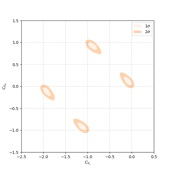
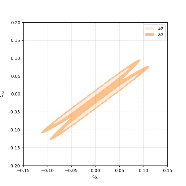
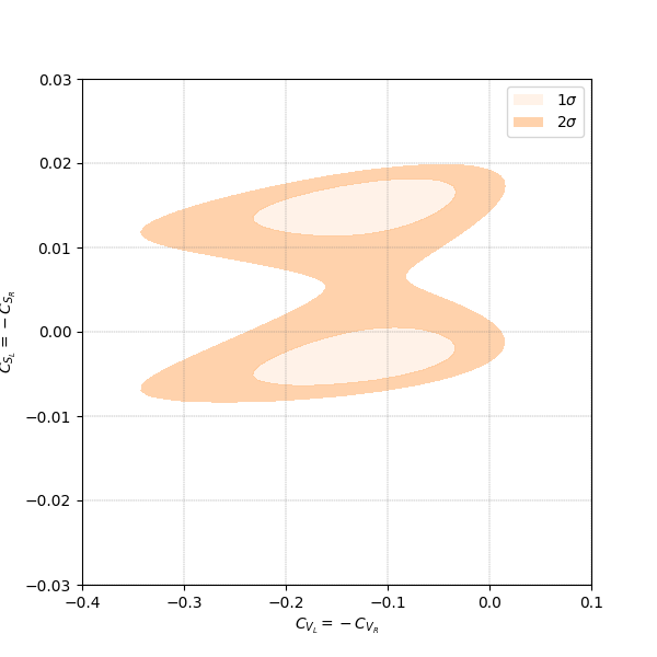
Figure 1: Contours for the allowed parameter space of $68\%$ (light orange area) and $95\%$ (orange area) for new Physics WCs obtained from our fit using the available measurements.

IV Angular Analysis in $\bar{B_{s}}\to K^{*+}(\to K\pi)\ell^{-}\bar{\nu}_{\ell}$

The fully differential decay rate for the semileptonic decay $\bar{B_{s}}\to K^{*+}(\to K\pi)\ell^{-}\bar{\nu}_{\ell}$ can be written similar to the decay rate of FCNC decay $B\to K^{*}(\to K\pi)\ell^{+}\ell^{-}$ [28]. The four body decay distribution for $\bar{B_{s}}\to K^{*+}(\to K\pi)\ell^{-}\bar{\nu}_{\ell}$ can be fully characterized by four kinematical variables : the invariant mass squared of the dilepton $(q^{2})$ and three angle variables $\theta_{\ell},\theta_{K^{*}}$ and $\phi$. Here, $\theta_{\ell}$ is the angle between $\ell$ in dilepton rest frame and direction opposite to B meson, $\theta_{K}$ is the angle between $K$ meson in $K^{*}$ rest frame and direction opposite to the B meson and $\phi$ is the angle between the plane defined by the dilepton and the plane defined by the $K\pi$ pair. The four fold differential distribution for this decay is given by

Figure 2: The kinematics of the semileptonic decay $\bar{B_{s}}\to K^{*+}(\to K\pi)\ell^{-}\bar{\nu}_{\ell}$

$$\frac{d^{4}\Gamma}{dq^{2}\,d\cos\theta_{\ell}\,d\cos\theta_{K^{*}}d\phi} \,=\,\frac{8\pi}{3}\Big{[}(J_{1s}+J_{2s}\cos\,2\theta_{\ell}+J_{3}\sin^{2}\theta_{\ell}\cos\,2\phi+J_{6s}\cos\theta_{\ell}$$ (7)

$$+J_{9}\sin^{2}\theta_{\ell}\sin\,2\phi)\sin^{2}\theta_{K^{*}}+(J_{1c}+J_{2c}\cos\,2\theta_{\ell})\cos^{2}\theta_{K^{*}}$$

$$+(J_{4}\sin\,2\theta_{\ell}\cos\phi+J_{5}\sin_{\theta_{\ell}}\cos\phi+J_{7}\sin\theta_{l}\sin\phi$$

$$+J_{8}\sin\,2\theta_{\ell}\sin\phi)\sin\,2\theta_{K^{*}}+J_{6c}\cos^{2}\theta_{K^{*}}\cos\theta_{\ell}\Big{]}$$

The coefficients $J_{i}(q^{2})$ are the function of dilepton invariant mass square and encapsulate the dynamic of the decay. These coefficients contain the form factors and are sensitive to different new physics. In the massless limit of lepton, these coefficients can be written as:

$$J_{1s} = \frac{3}{16}\Big{[}3{|\mathcal{A}^{L}_{\perp}|}^{2}+3{|\mathcal{A}^{L}_{\parallel}|}^{2}+16{|\mathcal{A}_{0\parallel}|}^{2}+16{|\mathcal{A}_{t\perp}|}^{2}\Big{]}$$

$$J_{1c} = \frac{3}{4}\Big{[}{|\mathcal{A}^{L}_{0}|}^{2}+2{|\mathcal{A}_{t}^{L}|}^{2}+8{|\mathcal{A}_{\parallel\perp}|}^{2}\Big{]}$$

$$J_{2s} = \frac{3}{16}\Big{[}{|\mathcal{A}^{L}_{\perp}|}^{2}+{|\mathcal{A}^{L}_{\parallel}|}^{2}-16{|\mathcal{A}_{0\parallel}|}^{2}-16{|\mathcal{A}_{t\perp}|}^{2}\Big{]}$$

$$J_{2c} = -\frac{3}{4}\Big{[}{|\mathcal{A}^{L}_{0}|}^{2}-8{|\mathcal{A}_{\parallel\perp}|}^{2}\Big{]}$$

$$J_{3} = \frac{3}{8}\Big{[}{|\mathcal{A}^{L}_{\perp}|}^{2}-{|\mathcal{A}^{L}_{\parallel}|}^{2}+16{|\mathcal{A}_{0\parallel|}}^{2}-16{|\mathcal{A}_{t\perp}|}^{2}\Big{]}$$

$$J_{4} = \frac{3}{4\sqrt{2}}\Big{[}\mathcal{A}^{L}_{0}{\mathcal{A}^{L}_{\parallel}}^{*}-8\sqrt{2}\mathcal{A}_{\parallel\perp}{\mathcal{A}_{0\parallel}}^{*}\Big{]}$$

$$J_{5} = \frac{3}{2\sqrt{2}}Re\Big{[}\mathcal{A}^{L}_{0}\mathcal{A}^{L}_{\perp}+2\sqrt{2}\mathcal{A}_{0\parallel}{\mathcal{A}^{L}_{t}}^{*}\Big{]}$$

$$J_{6s} = \frac{3}{2}Re\Big{[}\mathcal{A}^{L}_{\parallel}{\mathcal{A}^{L}_{\perp}}^{*}\Big{]}$$

$$J_{6c} = -6Re\Big{[}\mathcal{A}_{\parallel\perp}|{\mathcal{A}^{L}_{t}}^{*}\Big{]}$$

$$J_{7} = \frac{3}{2\sqrt{2}}Im\Big{[}\mathcal{A}^{L}_{0}{\mathcal{A}^{L}_{\parallel}}^{*}-2\sqrt{2}\mathcal{A}_{t\perp}{\mathcal{A}^{L}_{t}}^{*}\Big{]}$$

$$J_{8} = \frac{3}{4\sqrt{2}}Im\Big{[}\mathcal{A}^{L}_{0}{\mathcal{A}^{L}_{\perp}}^{*}\Big{]}$$

$$J_{9} = \frac{3}{4}Im\Big{[}\mathcal{A}^{L}_{\perp}{\mathcal{A}^{L}_{\parallel}}^{*}\Big{]}$$ (8)

The form factors of $B_{s}\to K^{*}$ are defined in appendix VI.1 and helicity amplitudes are given in appendix VI.2. The differential branching fraction $d\mathcal{B}/dq^{2}$ can be derived from equation 7 by integrating over the three angles in the range $\theta_{\ell}\in[0,\pi],\theta_{K^{*}}\in[0,\pi]$ and $\phi\in[0,2\pi]$

$$\frac{d\mathcal{B}}{dq^{2}}=\tau_{B}|N|^{2}\Big{[}2J_{1s}+J_{1c}-\frac{1}{3}\Big{(}2J_{2s}+J_{2c}\Big{)}\Big{]}$$ (9)

where the normalization factor is defined as

$$|N|^{2}=\frac{G_{F}^{2}\,V_{ub}^{2}\,q^{2}\sqrt{\lambda}}{3.2^{10}\pi^{3}M_{B_{s}}^{3}}$$ (10)

with $\lambda=\lambda(M_{B_{s}}^{2},M_{K^{*}}^{2},q^{2})$ which is the usual kinematic Kallen function.

The forward-backward asymmetry for lepton can be defined as

$$A_{FB}=\frac{\int_{0}^{1}\frac{d^{2}\Gamma}{dq^{2}\,d\cos\theta_{\ell}}d\cos\theta_{\ell}-\int_{-1}^{0}\frac{d^{2}\Gamma}{dq^{2}\,d\cos\theta_{\ell}}d\cos\theta_{\ell}}{\int_{-1}^{1}\frac{d^{2}\Gamma}{dq^{2}\,d\cos\theta_{\ell}}d\cos\theta_{\ell}}$$ (11)

After simplifying the above expression, this asymmetry can be expressed as given below

$$A_{FB}=\frac{J_{6s}+\frac{1}{2}J_{6c}}{\Big{[}2J_{1s}+J_{1c}-\frac{1}{3}\Big{(}2J_{2s}+J_{2c}\Big{)}\Big{]}}$$ (12)

The longitudinal polarization of $K^{*}$ meson can be written as :

$$F_{L}=\frac{3\Big{(}J_{1c}-\frac{1}{3}J_{2c}\Big{)}}{(2J_{1s}+J_{1c})-(2J_{2s}+J_{2c})}$$ (13)

We also define the integrated normalized angular observables as

$$\tilde{J}_{i}=\frac{\int_{q^{2}_{min}}^{q^{2}_{max}}J_{i}(q^{2})dq^{2}}{\int_{q^{2}_{min}}^{q^{2}_{max}}\frac{d\Gamma}{dq^{2}}dq^{2}}$$ (14)

The normalized angular obseravbles are independent from the value of CKM element $V_{ub}$.

V Predictions of observables in $\bar{B_{s}}\to K^{*+}(\to K\pi)\ell^{-}\bar{\nu}_{\ell}$

In this section, we explore the effects of NP WCs on the observables in the semileptonic decay $\bar{B_{s}}\to K^{*+}(\to K\pi)\ell^{-}\bar{\nu}_{\ell}$. We predict the observables differential branching ratio $\frac{d\mathcal{B}}{dq^{2}}$, lepton forward-backward asymmetry $A_{FB}$ and $K^{*}$ longitudinal polarization $F_{L}$ using the few best fit points of table 1. We have considered only those scenarios for the predictions which provides significant deviation from SM in the considered observables under the study. We can summarize the potential evidence of new physics in the predictions of the different observables:

• Differential branching fraction $\left(\frac{d\mathcal{B}}{dq^{2}}\right)$ : The differential branching fraction prediction plots for the three different scenario $S6,S7\,\&\,S17$ are given in FIG. 3. The SM band is shown in orange color where the band is due to the error in CKM and form factor parameters. We have considered the best fit points for the NP scenarios and the $1\sigma$ uncertainties in the hadronic form factors, together with CKM element error, are included for NP predictions. We find that all these scenarios can be distinguished from the SM as these scenarios provide the deviation from the SM prediction. We cannot distinguish these NP scenarios from each other as they provide the almost same type of deviation from SM. Also, the four benchmark points for scenario $S7$ provides the almost same $q^{2}$ spectrum.

  

  

  

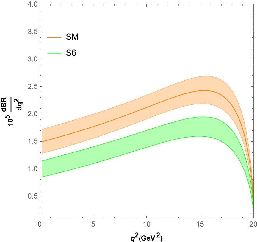
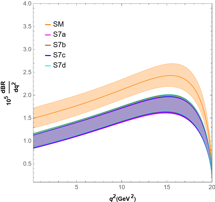
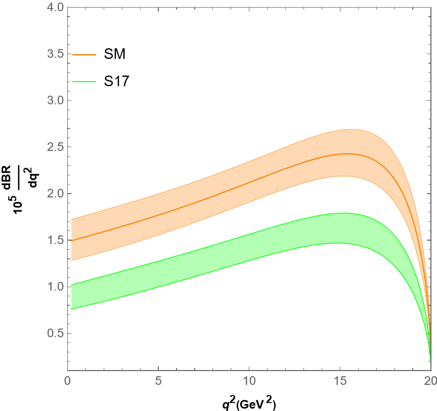
  Figure 3: Predictions of the differential branching fraction $dB/dq^{2}$ in $\bar{B_{s}}\to K^{*+}(\to K\pi)\ell^{-}\bar{\nu}_{\ell}$

• Leptonic forward-backward asymmetry $(A_{FB})$ : The predictions for lepton forward-backward asymmetry are shown in the FIG. 4. The NP scenarios $S6:C_{V_{L}}=-C_{V_{R}}$ and $S17:(C_{V_{L}}=-C_{V_{R}},C_{S_{L}}=-C_{S_{R}})$ provide small deviation from the SM in the forward-backward asymmetry. The two benchmark points (BPs) $S7a\,\&\,S7d$ for scenario $S7:(C_{V_{L}},C_{V_{R}})$ provide a small deviation from the SM but the other two scenarios $S7b\,\&\,S7c$ provide a large deviation in the forward-backward asymmetry. The BPs $S7a\,\&\,S7d$ provide the negative $A_{FB}$ for the whole $q^{2}$ range while $S7b\,\&\,S7c$ BPs give the positive $A_{FB}$ for the full $q^{2}$ range. The benchmark points $S7b\,\&\,S7c$ can be distinguished from the other two benchmark points $S7a\,\&\,S7d$ based on the forward-backward asymmetry which were indistinguishable from the differential branching fraction $\frac{d\mathcal{B}}{dq^{2}}$.

  

  

  

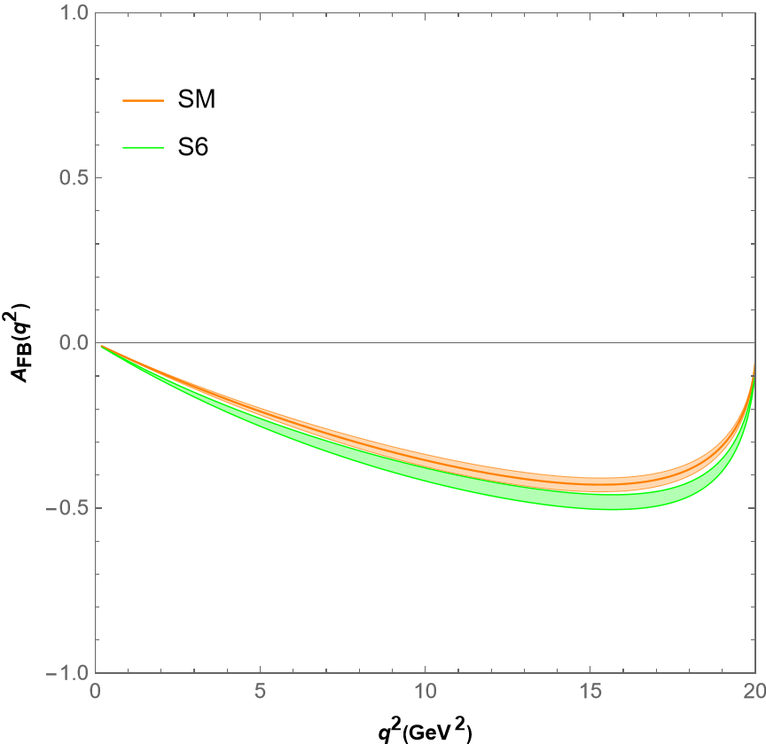
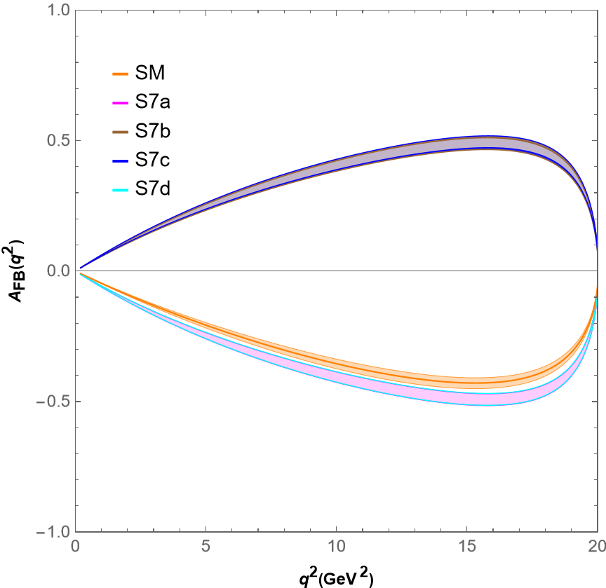
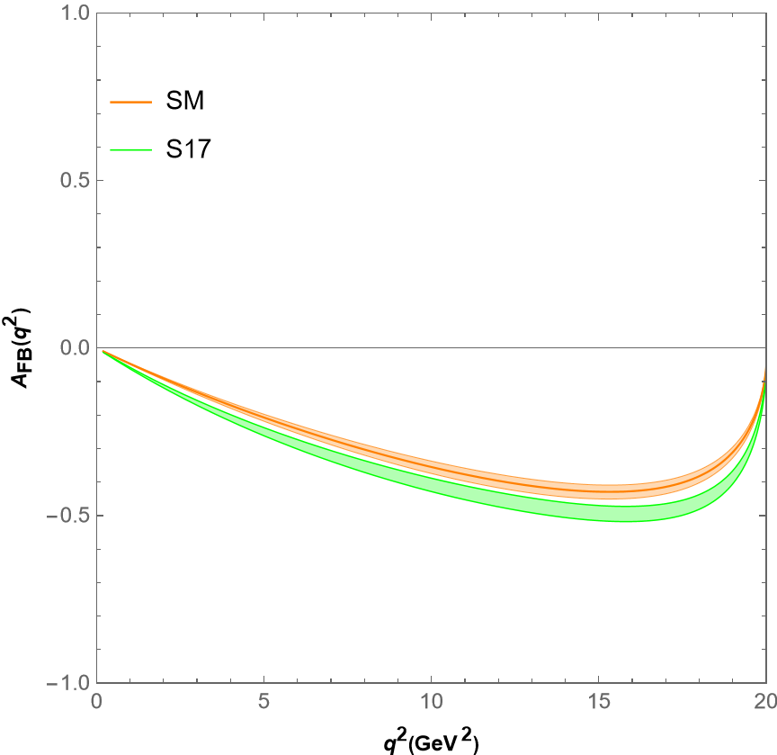
  Figure 4: Lepton forward-backward asymmetry $A_{FB}$ in $\bar{B_{s}}\to K^{*+}(\to K\pi)\ell^{-}\bar{\nu}_{\ell}$

• Longitudinal polarization of $K^{*}$ meson $(F_{L})$ : The prediction plots for longitudinal polarization fraction of $K^{*}$ meson are shown in FIG. 5. The NP scenarios provide a small deviation in the longitudinal polarization of $K^{*}$ meson. It is not possible to differentiate the NP scenarios with this observable.

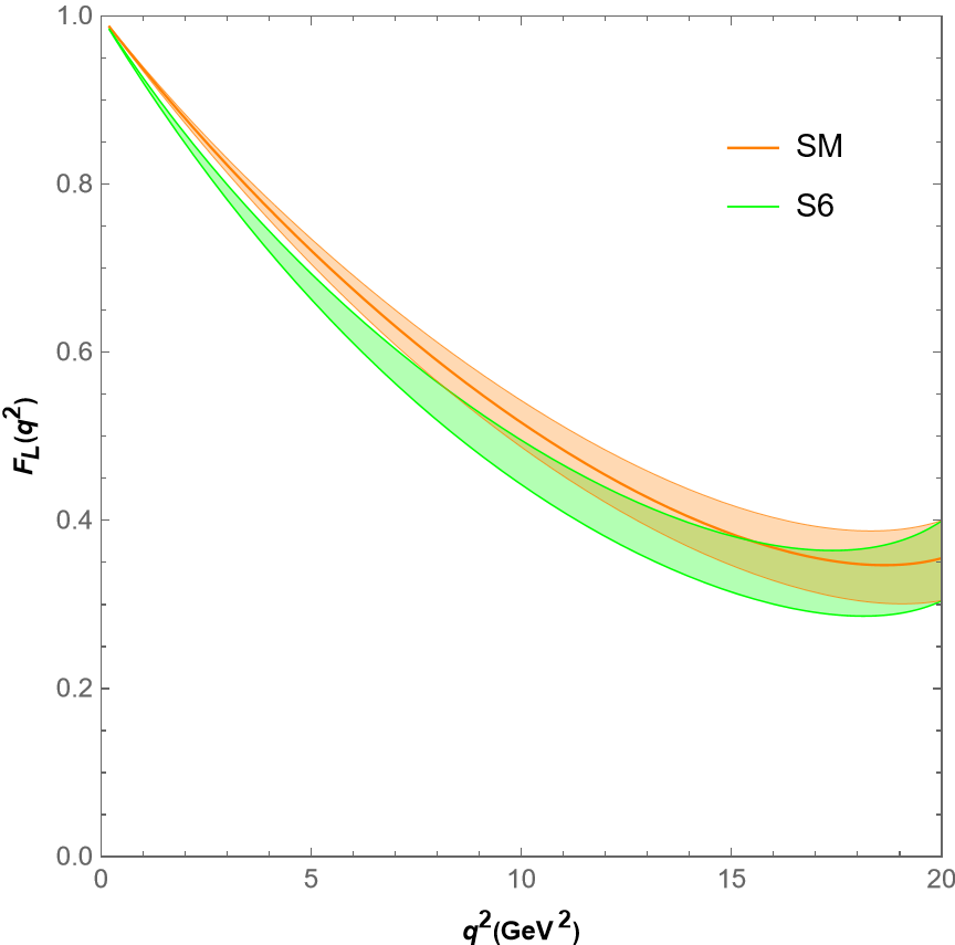
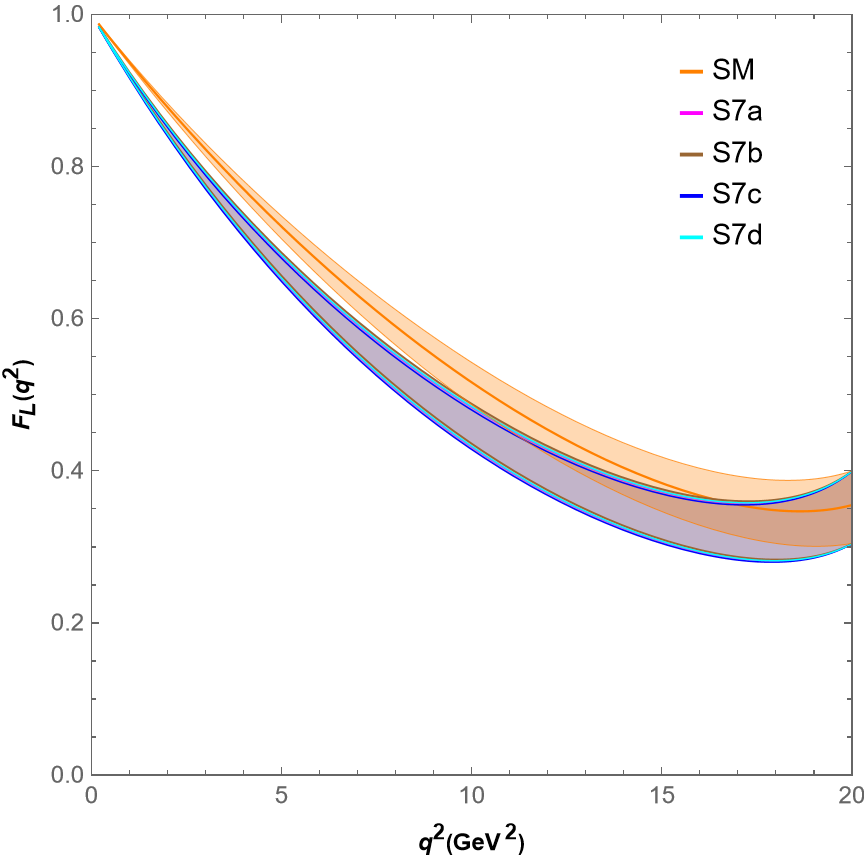
Figure 5: The predictions of the longitudinal polarization of $K^{*}$ meson $(F_{L})$ in $\bar{B_{s}}\to K^{*+}(\to K\pi)\ell^{-}\bar{\nu}_{\ell}$ decay

We also provide the prediction of the integrated values of the normalized angular obseravbles. We provide the integrated values for all the considered NP scenarios listed in table 1. The integrated values of these observables are given the Table 2 and Table 3

Scenario	$\tilde{J}_{1s}$	$\tilde{J}_{1c}$	$\tilde{J}_{2s}$	$\tilde{J}_{2c}$	$\tilde{J}_{3}$	$\tilde{J}_{4}$	$\tilde{J}_{5}$	$\tilde{J}_{6s}$
SM	0.255(35)	0.409(47)	0.085(12)	-0.409(47)	-0.059(23)	0.194(7)	-0.283(23)	-0.311(40)
$S1$	0.255(35)	0.409(47)	0.085(12)	-0.409(47)	-0.059(23)	0.194(7)	-0.283(23)	-0.311(40)
$S2$	0.269(36)	0.391(49)	0.090(12)	-0.391(49)	-0.039(28)	0.185(10)	-0.310(29)	-0.341(46)
$S3$	0.255(35)	0.409(47)	0.085(12)	-0.409(47)	-0.059(23)	0.194(7)	-0.283(23)	-0.311(40)
$S4$	0.255(35)	0.409(47)	0.085(12)	-0.409(47)	-0.059(23)	0.194(7)	-0.283(23)	-0.311(40)
$S5$	0.255(35)	0.409(47)	0.085(12)	-0.409(47)	-0.059(23)	0.194(7)	-0.283(23)	-0.311(40)
$S6$	0.267(38)	0.380(50)	0.092(12)	-0.380(50)	-0.028(31)	0.180(12)	-0.323(32)	-0.355(49)

Table 2: Predictions of the integrated value of the normalized angular observables in 1D NP scenarios

Scenario	$\tilde{J}_{1s}$	$\tilde{J}_{1c}$	$\tilde{J}_{2s}$	$\tilde{J}_{2c}$	$\tilde{J}_{3}$	$\tilde{J}_{4}$	$\tilde{J}_{5}$	$\tilde{J}_{6s}$
$\begin{matrix}S7a\\ S7b\\ S7c\\ S7d\\ \end{matrix}$	0.283(39)	0.373(51)	0.094(13)	-0.373(51)	-0.021(34)	0.177(14)	-0.331(34)	-0.364(51)
	0.280(38)	0.376(50)	0.093(12)	-0.376(50)	-0.024(33)	0.178(13)	0.328(34)	0.361(50)
	0.284(39)	0.371(52)	0.095(13)	-0.371(51)	-0.018(35)	0.176(14)	0.334(34)	0.367(51)
	0.282(38)	0.374(51)	0.094(12)	-0.374(51)	-0.021(34)	0.177(14)	-0.331(34)	-0.364(51)
$S8$	0.255(35)	0.409(47)	0.085(12)	-0.409(47)	-0.059(23)	0.194(7)	-0.283(23)	-0.311(40) )
$S9$	0.255(35)	0.409(47)	0.085(12)	-0.409(47)	-0.059(23)	0.194(7)	-0.283(23)	-0.311(40)
$S10$	0.255(35)	0.409(47)	0.085(12)	-0.409(48)	-0.059(23)	0.194(10)	-0.283(23)	-0.311(40)
$S11$	0.271(36)	0.389(49)	0.090(12)	-0.389(49)	-0.037(28)	0.184(10)	-0.312(30)	-0.343(48)
$S12$	0.271(36)	0.389(49)	0.090(12)	-0.389(49)	-0.037(28)	0.184(10)	-0.312(30)	-0.343(48)
$S13$	0.269(36)	0.391(49)	0.090(12)	-0.391(49)	-0.040(28)	0.185(11)	-0.310(30)	-0.340(47)
$S14$	0.255(35)	0.409(47)	0.085(12)	-0.409(47)	-0.059(23)	0.194(7)	-0.283(23)	-0.311(40)
$S15$	0.255(35)	0.409(47)	0.085 (12)	-0.409(48)	-0.059(23)	0.194(9)	-0.283(23)	-0.311(40)
$S16$	0.255(35)	0.409(47)	0.085(12)	-0.409(48)	-0.059(23)	0.194(9)	-0.283(23)	-0.311(40)
$S17$	0.284(39)	0.371(51)	0.095(13)	-0.371(51)	-0.018(34)	0.176(14)	-0.334(34)	-0.367(51)

Table 3: Predictions of the integrated value of the normalized angular observables in 2D NP scenarios

VI Conclusions

In this work, we consider the model independent approach to inspect the NP in leptonic and semileptonic decays of $B$ mesons induced by the quark level transition $b\to u\ell\nu_{\ell}$. We work in effective field theory by considering the general effective Hamiltonian with different NP Lorentz structures. We consider the NP operators with one at a time and two at a time scenarios. The different NP wilson coefficients in this analysis are constrained by using the available measurements in the $b\to u\ell\nu_{\ell}$ sector. The best fit of NP WCs are obtained by minimizing the $\chi^{2}$ function and we also obtain the contours for three 2D scenarios $S7:(C_{V_{L}},C_{V_{R}}),\,S14:(C_{S_{L}},C_{S_{R}})$ and $S17:(C_{V_{L}}=-C_{V_{R}},C_{S_{L}}=-C_{S_{R}})$.

The NP WCs are used to predict the possible departure from SM of obseravbles in $\bar{B_{s}}\to K^{*+}(\to K\pi)\ell^{-}\bar{\nu}_{\ell}$. We give the prediction of the $q^{2}$ spectrum of differential branching ratio, leptonic forward-backward asymmetry and longitudinal polarization of the $K^{*}$ meson in the semileptonic decay $\bar{B_{s}}\to K^{*+}(\to K\pi)\ell^{-}\bar{\nu}_{\ell}$ decay. Any deviation in the observables from the SM can indicate the presence of NP Lorentz structure. The NP scenarios $S6,S7$ and $S17$ decreases the differential $q^{2}$ spectrum from the SM. All these scenarios provide almost similar deviation in the branching ratio so it is not possible to distinguish them individually, but can be distinguished from the SM. The forward-backward asymmetry of lepton with NP effects also deviates from the SM prediction and the two benchmark points $S7a\,\&\,S7d$ of $S7:(C_{V_{L}},C_{V_{R}})$ scenario can be distinguished from the other benchmark points $S7b\,\&\,S7c$ as these two give the positive value of $A_{FB}(q^{2})$ in the full $q^{2}$ range whereas the other benchmark points provide the negative $A_{FB}$. The lepton polarization fraction of $K^{*}$ meson also deviates from the SM. We also provided the predictions for the integrated values of the normalized angular observables for both 1D and 2D NP scenarios in this decay.

Appendix

VI.1 $B_{s}\to K^{*}$ transition form factors

The hadronic matrix elements for $B_{s}\to K^{*}$ can be written in terms of seven form factors, namely $V,A_{0},A_{1},A_{12},T_{1},T_{2}$ and $T_{23}$. The form factors are defined by simplified series expansion in $z$ given by Bharucha-Straub-Zwicky [27] as

$$f_{i}(q^{2})=\frac{1}{(1-q^{2}/m_{R,i}^{2})}\sum_{k}\alpha_{k}^{i}[z(q^{2})-z(0)]^{k}$$ (15)

where the parameters $z(q^{2})$ is defined as

$$z(t)=\frac{\sqrt{t_{+}-t}-\sqrt{t_{+}-t_{0}}}{\sqrt{t_{+}-t}+\sqrt{t_{+}-t_{0}}}$$ (16)

with $t_{\pm}=(m_{B_{s}}\pm m_{K^{*}})$ and $t_{0}=(m_{B_{s}}+m_{K^{*}})(\sqrt{m_{B_{s}}}-\sqrt{m_{K^{*}}})^{2}$. The fit results for the SSE expansion coefficients using the combined LCSR + Lattice fit and masses of sub-thresold resonances are provided in Ref. [27]. We have summarized these resonance masses and SSE expansion coefficients in table 4 and table 5, respectively.

$f_{i}$	$J^{P}$	$m_{R,i}/GeV$
$A_{0}$	$0^{-}$	5.279
$V,T_{1}$	$1^{-}$	5.325
$A_{1},T_{2},A_{12},T_{23}$	$1^{+}$	5.724

Table 4: Masses of resonances required for form factor parameterizations [27]

$f_{i}$	$\alpha_{0}^{i}$	$\alpha_{1}^{i}$	$\alpha_{2}^{i}$
$V$	$0.28\pm 0.02$	$-0.82\pm 0.19$	$5.08\pm 1.42$
$A_{0}$	$0.36\pm 0.02$	$-0.36\pm 0.20$	$8.03\pm 2.07$
$A_{1}$	$0.22\pm 0.01$	$0.24\pm 0.16$	$1.77\pm 0.85$
$A_{12}$	$0.27\pm 0.02$	$1.12\pm 0.11$	$3.43\pm 0.78$
$T_{1}$	$0.24\pm 0.01$	$-0.75\pm 0.15$	$2.49\pm 1.37$
$T_{2}$	$0.24\pm 0.01$	$0.31\pm 0.15$	$1.58\pm 0.93$
$T_{23}$	$0.60\pm 0.04$	$2.40\pm 0.27$	$9.64\pm 2.03$

Table 5: Simplified series expansion coefficients $\alpha_{k}^{i}$ for parameterising the $B_{s}\to K^{*}$ form factors [27]

The form factors for vector currents, axial vector currents and tensor currents in the helicity basis can be written as [16]

• Vector current

  $$\mathcal{F}_{\perp}(q^{2})=\dfrac{\sqrt{2\lambda}}{M_{B_{s}}(M_{B_{s}}+M_{K^{*}})}V(q^{2})$$ (17)

• Axial vector current

  $$\mathcal{F}_{t}(q^{2}) =\dfrac{\sqrt{\lambda}}{{M_{B_{s}}}^{2}}A_{0}(q^{2})$$ (18)

  $$\mathcal{F}_{\parallel}(q^{2}) =\sqrt{2}\frac{M_{B_{s}}+M_{K^{*}}}{M_{B_{s}}}A_{1}(q^{2})$$ (19)

  $$\mathcal{F}_{0}(q^{2}) =\dfrac{8M_{K^{*}}A_{12}(q^{2})}{M_{B_{s}}}$$ (20)

• Tensor current

  $$\mathcal{F}_{\perp}^{T}(q^{2}) =\dfrac{\sqrt{2\lambda}}{{M_{B_{s}}}^{2}}T_{1}(q^{2})$$ (21)

  $$\mathcal{F}_{\parallel}^{T}(q^{2}) =\dfrac{\sqrt{2}({M_{B_{s}}}^{2}-{M_{K^{*}}}^{2})}{{M_{B_{s}}}^{2}}T_{2}(q^{2})$$ (22)

  $$\mathcal{F}^{T}_{0}(q^{2}) =\dfrac{4M_{K^{*}}T_{23}(q^{2})}{M_{B_{s}}+M_{K^{*}}}$$ (23)

VI.2 Helicity amplitudes

The helicity amplitudes for $\bar{B_{s}}\to K^{*+}(\to K\pi)\ell^{-}\bar{\nu}_{\ell}$ are given as [16]

$$\mathcal{A}_{0}^{L} =-4\dfrac{M_{B_{s}}^{2}(1+C_{V_{L}}-C_{V_{R}})\mathcal{F}_{0}(q^{2})}{\sqrt{q^{2}}}$$ (24)

$$\mathcal{A}_{\perp}^{L} =4M_{B_{s}}(1+C_{V_{L}}+C_{V_{R}})\mathcal{F}_{\perp}(q^{2})$$ (25)

$$\mathcal{A}_{\parallel}^{L} =-4M_{B_{s}}(1+C_{V_{L}}-C_{V_{R}})\mathcal{F}_{\parallel}(q^{2})$$ (26)

$$\mathcal{A}_{t}^{L} =-4\big{[}{\dfrac{m_{l}M_{B_{s}}^{2}}{\sqrt{q^{2}}}}(1+C_{V_{L}}-C_{V_{R}})+\dfrac{M_{B_{s}}^{2}}{m_{b}}(C_{S_{L}}-C_{S_{R}})\big{]}\mathcal{F}_{t}(q^{2})$$ (27)

$$\mathcal{A}_{\parallel\perp} =+8M_{B_{s}}C_{T}\mathcal{F}_{0}^{T}(q^{2})$$ (28)

$$\mathcal{A}_{t\perp} =4\sqrt{2}\dfrac{M_{B_{s}}^{2}}{\sqrt{q^{2}}}C_{T}\mathcal{F}_{\perp}^{T}(q^{2})$$ (29)

$$\mathcal{A}_{0\parallel} =4\sqrt{2}\dfrac{M_{B_{s}}^{2}}{\sqrt{q^{2}}}C_{T}\mathcal{F}_{\parallel}^{T}(q^{2})$$ (30)

References

- [1] R. Aaij et al. [LHCb], “Measurement of the branching fraction ratios and using muonic decays,” [arXiv:2406.03387 [hep-ex]].
- [2] https://hflav-eos.web.cern.ch/hflav-eos/semi/moriond24/html/RDsDsstar/RDRDs.html
- [3] J. P. Lees et al. [BaBar], “Evidence for an excess of decays,” Phys. Rev. Lett. 109 (2012), 101802 doi:10.1103/PhysRevLett.109.101802 [arXiv:1205.5442 [hep-ex]].
- [4] J. P. Lees et al. [BaBar], “Measurement of an Excess of Decays and Implications for Charged Higgs Bosons,” Phys. Rev. D 88 (2013) no.7, 072012 doi:10.1103/PhysRevD.88.072012 [arXiv:1303.0571 [hep-ex]].
- [5] M. Huschle et al. [Belle Collaboration], “Measurement of the branching ratio of relative to decays with hadronic tagging at Belle”, Phys. Rev. D 92, no. 7, 072014 (2015) [arXiv:1507.03233 [hep-ex]].
- [6] S. Hirose et al. [Belle Collaboration], “Measurement of the lepton polarization and in the decay ”, Phys. Rev. Lett. 118, no. 21, 211801 (2017) [arXiv:1612.00529 [hep-ex]].
- [7] S. Hirose et al. [Belle], “Measurement of the lepton polarization and in the decay with one-prong hadronic decays at Belle,” Phys. Rev. D 97 (2018) no.1, 012004 doi:10.1103/PhysRevD.97.012004 [arXiv:1709.00129 [hep-ex]].
- [8] G. Caria et al. [Belle], “Measurement of and with a semileptonic tagging method,” Phys. Rev. Lett. 124 (2020) no.16, 161803 doi:10.1103/PhysRevLett.124.16180 3 [arXiv:1910.05864 [hep-ex]].
- [9] I. Adachi et al. [Belle-II], “A test of lepton flavor universality with a measurement of using hadronic tagging at the Belle II experiment,” [arXiv:2401.02840 [hep-ex]].
- [10] R. Aaij et al. [LHCb], “Measurement of the ratios of branching fractions and ,” Phys. Rev. Lett. 131 (2023), 111802 doi:10.1103/PhysRevLett.131.111802 [arXiv:2302.02886 [hep-ex]].
- [11] R. Aaij et al. [LHCb], “Test of lepton flavor universality using B0→D*-+ decays with hadronic channels,” Phys. Rev. D 108 (2023) no.1, 012018 [erratum: Phys. Rev. D 109 (2024) no.11, 119902] doi:10.1103/PhysRevD.108.012018 [arXiv:2305.01463 [hep-ex]].
- [12] S. Iguro, T. Kitahara and R. Watanabe, “Global fit to b→c anomalies as of Spring 2024,” Phys. Rev. D 110 (2024) no.7, 7 doi:10.1103/PhysRevD.110.075005 [arXiv:2405.06062 [hep-ph]].
- [13] W. F. Duan, S. Iguro, X. Q. Li, R. Watanabe and Y. D. Yang, “Sum rules for semi-leptonic and decays: accuracy checks and implications,” [arXiv:2410.21384 [hep-ph]].
- [14] A. Greljo, J. Salko, A. Smolkovič and P. Stangl, “SMEFT restrictions on exclusive b → u decays,” JHEP 11 (2023), 023 doi:10.1007/JHEP11(2023)023 [arXiv:2306.09401 [hep-ph]].
- [15] D. Leljak, B. Melić, F. Novak, M. Reboud and D. van Dyk, “Toward a complete description of b → u decays within the Weak Effective Theory,” JHEP 08 (2023), 063 doi:10.1007/JHEP08(2023)063 [arXiv:2302.05268 [hep-ph]].
- [16] T .Feldmann, B. Müller and D. van Dyk, “Analyzing transitions in semileptonic decays,” Phys. Rev. D 92 (2015) no.3, 034013 doi:10.1103/PhysRevD.92.034013 [arXiv:1503.09063 [hep-ph]].
- [17] Y. S. Amhis et al. [HFLAV], “Averages of b-hadron, c-hadron, and -lepton properties as of 2021,” Phys. Rev. D 107 (2023) no.5, 052008 doi:10.1103/PhysRevD.107.052008 [arXiv:2206.07501 [hep-ex]].
- [18] P. del Amo Sanchez et al. [BaBar], “Study of and Decays and Determination of ,” Phys. Rev. D 83 (2011), 032007 doi:10.1103/PhysRevD.83.032007 [arXiv:1005.3288 [hep-ex]].
- [19] J. P. Lees et al. [BaBar], “Branching fraction and form-factor shape measurements of exclusive charmless semileptonic B decays, and determination of ,” Phys. Rev. D 86 (2012), 092004 doi:10.1103/PhysRevD.86.092004 [arXiv:1208.1253 [hep-ex]].
- [20] H. Ha et al. [Belle], “Measurement of the decay and determination of ,” Phys. Rev. D 83 (2011), 071101 doi:10.1103/PhysRevD.83.071101 [arXiv:1012.0090 [hep-ex]].
- [21] A. Sibidanov et al. [Belle], “Study of Exclusive Decays and Extraction of using Full Reconstruction Tagging at the Belle Experiment,” Phys. Rev. D 88 (2013) no.3, 032005 doi:10.1103/PhysRevD.88.032005 [arXiv:1306.2781 [hep-ex]].
- [22] J. P. Lees et al. [BaBar], “Branching fraction measurement of decays,” Phys. Rev. D 87 (2013) no.3, 032004 [erratum: Phys. Rev. D 87 (2013) no.9, 099904] doi:10.1103/PhysRevD.87.032004 [arXiv:1205.6245 [hep-ex]].
- [23] M. T. Prim et al. [Belle], “Search for and with inclusive tagging,” Phys. Rev. D 101 (2020) no.3, 032007 doi:10.1103/PhysRevD.101.032007 [arXiv:1911.03186 [hep-ex]].
- [24] M. Tanaka and R. Watanabe, “New physics in the weak interaction of ,” Phys. Rev. D 87 (2013) no.3, 034028 doi:10.1103/PhysRevD.87.034028 [arXiv:1212.1878 [hep-ph]].
- [25] Y. Sakaki, M. Tanaka, A. Tayduganov and R. Watanabe, “Testing leptoquark models in ,” Phys. Rev. D 88 (2013) no.9, 094012 doi:10.1103/PhysRevD.88.094012 [arXiv:1309.0301 [hep-ph]].
- [26] D. Leljak, B. Melić and D. van Dyk, “The → form factors from QCD and their impact on —Vub—,” JHEP 07 (2021), 036 doi:10.1007/JHEP07(2021)036 [arXiv:2102.07233 [hep-ph]].
- [27] A. Bharucha, D. M. Straub and R. Zwicky, “ in the Standard Model from light-cone sum rules,” JHEP 08 (2016), 098 doi:10.1007/JHEP08(2016)098 [arXiv:1503.05534 [hep-ph]].
- [28] S. Jäger and J. Martin Camalich, “On at small dilepton invariant mass, power corrections, and new physics,” JHEP 05 (2013), 043 doi:10.1007/JHEP05(2013)043 [arXiv:1212.2263 [hep-ph]].