Formal Logic-guided Robust Federated Learning against Poisoning Attacks

Abstract

Federated Learning (FL) offers a promising solution to the privacy concerns associated with centralized Machine Learning (ML) by enabling decentralized, collaborative learning. However, FL is vulnerable to various security threats, including poisoning attacks, where adversarial clients manipulate the training data or model updates to degrade overall model performance. These attacks can introduce critical malfunctions, such as biased predictions or reduced accuracy, undermining the integrity and robustness of the global model. Recognizing this threat, researchers have focused on developing defense mechanisms to counteract poisoning attacks in FL systems. However, existing robust FL methods predominantly focus on computer vision tasks, leaving a gap in addressing the unique challenges of FL with time series data. These tasks, which often involve sequential dependencies and temporal patterns, have been largely overlooked in the context of poisoning attack defenses.

In this paper, we present FLORAL, a defense mechanism designed to mitigate poisoning attacks in federated learning for time-series tasks, even in scenarios with heterogeneous client data and a large number of adversarial participants. Based on our investigation of the effectiveness of poisoning attack defenses within the Federated Time Series (FTS) domain, we pinpoint the limitations of mainstream defenses against such attacks. Unlike traditional model-centric defenses, FLORAL leverages logic reasoning to evaluate client trustworthiness by aligning their predictions with global time-series patterns, rather than relying solely on the similarity of client updates. Our approach extracts logical reasoning properties from clients, then hierarchically infers global properties, and uses these to verify client updates. Through formal logic verification, we assess the robustness of each client contribution, identifying deviations indicative of adversarial behavior. Experimental results on two datasets demonstrate the superior performance of our approach compared to existing baseline methods, highlighting its potential to enhance the robustness of FL to time series applications. Notably, FLORAL reduced the prediction error by 93.27% in the best-case scenario compared to the second-best baseline. Our code is available at https://anonymous.4open.science/r/FLORAL-Robust-FTS.

I Introduction

Federated Learning (FL) has emerged as a promising solution that enables using data and computing resources from multiple clients to train a shared model under the orchestration of a central server [33]. In FL, clients use their data to train the model locally and iteratively share the local updates with the server, which then combines the contributions of the participating clients to generate a global update. The security aggregation mechanism and its distinctive distributed training mode render it highly compatible with a wide range of practical applications that have stringent privacy demands [49, 59, 40, 21]. Recently, FL has been demonstrated to be efficient in time-series related tasks [10, 48, 3] to securely share knowledge of similar expertise among different tasks and protect user privacy. Although FL has many notable characteristics and has been successful in many applications [2, 21, 46, 52, 66, 22, 41], recent studies indicate that FL is fundamentally susceptible to adversarial attacks in which malicious clients manipulate the local training process to contaminate the global model [6, 55, 44]. Based on the attack’s goal, adversarial attacks can be broadly classified into untargeted and targeted attacks. The former aims to deteriorate the performance of the global model on all test samples [9, 14]; while the latter focuses on causing the model to generate false predictions following specific objectives of the adversaries [62, 6].

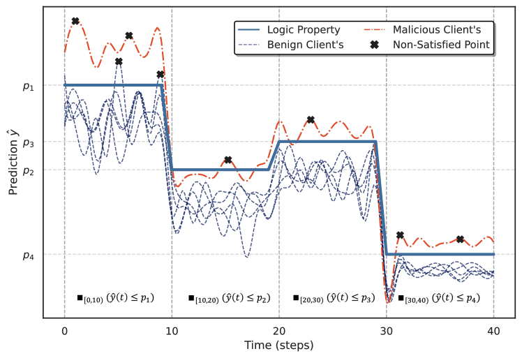
Figure 1: Illustration of logical verification given by benign and malicious clients’ predictions. The global property here is $\square_{(0,10]}(\hat{y}(t)\leq p_{1})\wedge\square_{(10,20]}(\hat{y}(t)\leq p_{2})\wedge\square_{(20,30]}(\hat{y}(t)\leq p_{3})\wedge\square_{(30,40]}(\hat{y}(t)\leq p_{4})$. Examples of points violating this property are marked with x.

Many efforts have been devoted to dealing with existing threats in FL, which can be roughly classified into two directions: robust FL aggregation [50, 47, 69, 71] and anomaly model detection. The former aims to optimize the aggregation function to limit the effects of polluted updates caused by attackers, whereas the latter attempts to identify and remove malicious updates. For instance, Xie et al. [69] presented a certified defense mechanism based on the clipping and perturbation paradigm. Other approaches focused on new estimators such as coordinate-wise median, $\alpha$-trimmed mean [72], and geometric median [50] for aggregation. The main drawback of the methods mentioned above is that polluted updates remain in the global model, reducing the model’s precision while not mitigating the attack impact [43]. Several methods have been proposed to identify and remove adversarial clients from the aggregation [9, 60, 42, 54, 17, 73]. In [60], the authors proposed a defense mechanism against poisoning attacks in collaborative learning based on the $K$-Means algorithm. Sattler et al. [57] proposed dividing the clients’ updates into normal updates and suspicious updates based on their cosine similarities. However, most methods for identifying malicious clients proposed so far follow the majority-based paradigm in that they assume benign local model updates are a majority compared to the malicious ones; thus, polluted updates are supposed to be outliers in the distribution of all updates. Unfortunately, this hypothesis holds only if the data of the clients is IID (independent and identically distributed) and the number of malicious clients is small. Though these two approaches can mitigate poisoning attacks in FL, most of them have been evaluated primarily in the context of computer vision tasks, where image-based datasets dominate the landscape [17, 47, 44, 63]. However, FL applied to time-series data remains underexplored, particularly regarding its vulnerabilities, where adversarial attacks pose a significant threat, much like those observed in image-based datasets [23, 12, 13, 38]. Given the critical applications of time-series analysis, such as in healthcare [5, 36], financial systems [35, 34], and industrial monitoring [31, 30], ensuring the robustness and security of FL models in these scenarios is of paramount importance. Our empirical result demonstrates that these methods are not effective in the scenario of FL with time-series tasks where the data itself reflects a high level of non-iid due to the different locations where it is collected.

To fill this gap, we propose FLORAL, a defense mechanism capable of mitigating poisoning attacks against Federated Time Series (FTS) under the most challenging scenarios, i.e., in the presence of heterogeneous client data and a large number of adversarial clients. Our approach is orthogonal to existing model-centric defenses. Instead, we rely on logic-based reasoning to evaluate the reliability of clients based on their behavior and resistance to poisoning attacks. This approach assesses the trustworthiness of clients by aligning their predictions with global time-series patterns. Specifically, we use symbolic reasoning to capture the logical semantics embedded in time series data, which has been shown to improve the learning process and produce more robust models for future predictions [3, 31, 29]. Our FL defense method builds on this by using symbolic reasoning to evaluate diverging intra-task logic patterns in client predictions, allowing for the detection of anomalous clients without relying solely on model similarity. This highlights the enhanced effectiveness of reasoning logic in identifying malicious behaviors in FL. The intuition behind our approach is that, after rounds of training, benign models naturally converge toward the same global objective and share consistent logical reasoning patterns, while malicious models diverge, aiming to manipulate global behavior and thereby exhibit deviant reasoning patterns. The high-level idea is visualized in Figure 1. In centralized FL, we expect the final model $G_{T}$ to have the minimized error on the local data, with local models converging on a unified objective [49, 27, 24]. In light of these findings, we propose FLORAL, a logic-guided defense for FL which includes three key components. First, we extract logical reasoning properties (e.g., when training models relating to traffic and driving, a dataset measuring vehicle density over time would by expected to reach an upper extreme value of, say, 100) from clients and apply hierarchical clustering to group client updates based on the logical properties of their local models. This allows us to infer the global reasoning properties that represent the system’s clients based on clustered properties. These formal logic properties rigorous assessment of the consistency and validity of client contributions by identifying deviations from expected model behaviors. This verification-based defense substantially strengthens the security of federated learning in time-series applications, where the risk of undetected adversarial behavior is particularly high due to the sensitive nature of these tasks. By optimizing for the unique challenges of time-series data, our method enhances the robustness of FL systems, providing a more reliable safeguard compared to existing defenses. Experimental results validate the effectiveness of our approach in mitigating poisoning attacks while maintaining high model performance.

In summary, our contributions are specified as follows:

• We introduce FLORAL — a novel poisoning-resistant defense for FL. It identifies and eliminates suspicious clients that distort the global model using logical reasoning property inference and verification. FLORAL is the first work that, to the best of our knowledge, thoroughly addresses poisoning attacks in FTS, even in the presence of a large number of compromised participants and complicated attack strategies.

• We are the first to study the efficacy of existing robust FL defenses in the context of FTS and pinpoint their limitation when adapted to the time-series domain.

• We conduct comprehensive experiments and in-depth studies on various datasets, FL settings, and attack scenarios to demonstrate the superiority of FLORAL over state-of-the-art defense techniques.

II Related Works

In this section, we first discuss adversarial attacks in FL to distinguish them from those from centralized ML; then we present mainstream FL defenses against adversarial attacks.

II-A Poisoning Attacks in FL

Unlike traditional centralized learning, where data is aggregated in a single location, FL operates under a decentralized paradigm where data remains on client devices and only model updates are shared with a central server. This distributed nature makes FL susceptible to various types of poisoning attacks [39, 25]. A poisoning attack in federated learning occurs when an attacker alters the model submitted by a client to the central server during the aggregation process, either directly or indirectly, causing the global model to update incorrectly [67].

Depending on the goal of a poisoning attack, we can classify poisoning attacks into two categories: (1) untargeted poisoning attacks [19, 9], and (2) targeted poisoning attacks [58, 64, 70]. Untargeted poisoning attacks aim to make the learned model have a high testing error indiscriminately for testing examples, which eventually results in a denial-of-service attack. Byzantine attack is among the most popular such attacks [9, 61]. In targeted poisoning attacks, the learned model produces attacker-desired predictions for particular testing examples, e.g., predicting spam as non-spam and predicting attacker-desired labels for testing examples with a particular trojan trigger (these attacks are also known as backdoor/trojan attacks [44]). In the context of a time-series task, the targeted attack can be adding imperceptible noise to the original sample such that the model predicts the incorrect class [53] or manipulating the prediction into the extreme value/specific directions [38].

To further strengthen the attack, some model poisoning attacks are often combined with data poisoning ones [44, 6]. In such attacks, adversaries intentionally manipulate their local model updates before sending them to the central server. In [8, 45], the projected gradient descent (PGD) attack is introduced to be more resistant to many defense mechanisms. In a PGD attack, the attacker projects their model on a small ball centered around the previous iteration’s global model. In addition, scaling and constraining-based techniques [15, 26] are commonly used to intensify the poisoning effect while stealthily bypassing robust aggregators.

II-B Defenses against Poisoning Attacks in FL

Defending against poisoning attacks in Federated Learning requires novel approaches tailored to the unique characteristics of the FL paradigm. Existing defense strategies can be broadly categorized into (1) robust aggregation mechanisms, (2) anomaly detection, and (3) adversarial training. Robust Aggregation Mechanisms are designed to mitigate the impact of malicious updates during the model aggregation process [47, 9, 50, 71]. Blanchard et al. [9] proposed the Krum algorithm, which selects updates from a majority of clients that are most similar to each other, thereby excluding potentially malicious updates. Another approach, Median-based aggregation [50, 72], takes the median of the updates from all clients, which is more resilient to outliers and adversarial manipulations. RLR [47] adjusts the global learning rate based on the sign information contained within each update per dimension and combines the differential privacy noising.

The second approach is backdoor detection, which detects the backdoor gradients and filters them before aggregation [9, 73, 17, 18, 37, 42]. To begin, Cao et al. [11] introduced FLTrust, a method that establishes a trust score for each client based on the similarity of their updates to a trusted server-side model. Updates with low trust scores are either down-weighted or excluded from the aggregation process. More recently, Zhang et al. [73] proposed to predict a client’s model update in each iteration based on historical model updates and then flag a client as malicious if the received model update from the client and the predicted model update is inconsistent in multiple iterations. In addition Nguyen et al. [42] developed an approach that combines anomaly detection with clustering, grouping similar updates and filtering out those that deviate significantly from the majority.

To this end, the effectiveness of these methods in Federated Time Series (FTS) scenarios remains unclear, as they lack components specifically designed to capture and investigate logical reasoning properties inherent in time-series data. Time series data introduces unique temporal dependencies and patterns that may require additional strategies to accurately detect adversarial behavior. Existing defenses, being largely model-centric, do not account for the temporal relationships or dynamic changes in the data, which are critical for ensuring robust performance in FTS. As a result, new approaches that integrate logical reasoning and temporal consistency checks are needed to enhance adversarial defenses in such contexts.

III Background

In this section, we first provide the formulation of FTS and the threat model which is addressed in our method; then provide the background on logical reasoning property inference and verification — the key components of FLORAL.

III-A Federated Time Series (FTS)

This work focuses on time series forecasting, which involves predicting future values based on historical data. Formally, let $\mathbf{X}_{1:L}=\left(\mathbf{x}_{1},\cdots,\mathbf{x}_{L}\right)^{\top}\in\mathbb{R}^{L\times M}$ be a history sequence of $L$ multivariate time series, where for any time step $t$, each row $\mathbf{x}_{t}=$ $\left(x_{t1},\ldots,x_{tM}\right)\in\mathbb{R}^{1\times M}$ is a multivariate vector consisting of $M$ variables or channels. Given a history sequence $\mathbf{X}_{1:L}$ with look-back window $L$, the goal of multivariate time series forecasting is to predict a sequence $\mathbf{X}_{L+1:L+\tau}=\left(\mathbf{x}_{L+1},\ldots,\mathbf{x}_{L+\tau}\right)^{\top}\in\mathbb{R}^{\tau\times M}$ for the future $\tau$ timesteps.

To achieve this in a decentralized and privacy-preserving manner, we consider a federated learning (FL) system where $N$ participants collaborate to build a global model $G_{T}$ that generalizes well to their future observations. In our FL system, there is a central server $\mathcal{S}$ and a client pool $\mathcal{C}=[C_{1},C_{2},\ldots,C_{N}]$, where each client $i$ has a dataset of size $|\mathcal{D}_{i}|=N_{i}$. The training procedure involves $T$ rounds of interaction between the server and the clients:

• The server broadcasts the current global model $G^{t-1}$ to all participating clients. Note the initial model $G^{0}$ is randomly initialized.

• Each client $i$ updates the global model $G^{t-1}$ using its local dataset $\mathcal{D}_{i}$ via mini-batch stochastic gradient descent (SGD) and sends its updated model weights back to the server.

• The server aggregates the local updates $G^{t}_{i}$ from all clients to generate a new global model $G^{t}$, which is then shared with the clients in the next round.

This iterative process continues until the global model achieves satisfactory performance on all clients’ data, ensuring it generalizes well across the diverse datasets in the federated setting.

III-B Threat Model

TABLE I: Examples of temporal reasoning templates specified with STL.

Reasoning Property	Description	Templatized Logic Formula	Parameters
Operational Range	Signal is upper-bounded by threshold $a$ and lower-bounded by threshold $b$.	$\bigwedge_{i=1}^{1,2,...,\tau}(\square_{[i,i+t]}(x\leq a_{i}\wedge x\geq b_{i}))$	$a_{i},b_{i}$
Existence	Signal should eventually reach the upper extreme $a$ and the lower extreme $b$.	$\bigwedge_{i=1}^{1,2,...,\tau}(\Diamond_{[i,i+t]}(x\leq a_{i}\wedge x\geq b_{i}))$	$a_{i},b_{i}$
Until	Signal must satisfy one specification at all times until another condition is met.	$\bigwedge_{i=1}^{1,2,...,t}((x<a_{i})\,\mathcal{U}_{[i,i+1]}(x<b_{i}))$	$a_{i},b_{i}$
Intra-task Reasoning	The difference between signal variables $x_{1}$ and $x_{2}$ should be greater than $a$.	$\bigwedge_{i=1}^{1,2,...,\tau}(\square_{[i,i+t]}((x_{1}-x_{2})>a_{i}))$	$a_{i}$
Temporal Implications	The happening of one event indicates that another event will happen at some point in the future.	$\square_{[t_{1},t_{2}]}((x\geq a_{1})\rightarrow\Diamond_{[t_{3},t_{4}]}(x\geq a_{2}))$	$a_{1},a_{2}$
Intra-task Nested Reasoning	The signal variable $x_{1}$, when greater than a threshold $a$, indicates $x_{2}$ will eventually reach a threshold $b$	$\square_{[t_{1},t_{2}]}((x_{1}\geq a)\rightarrow\Diamond_{[t_{3},t_{4}]}(x_{2}\geq b))$	$a,b$
Multiple Eventualities	Multiple events must eventually happen, but their order can be arbitrary.	$\Diamond_{[t_{1},t_{2}]}(x\geq a_{1})\wedge\cdots\wedge\Diamond_{[t_{3},t_{4}]}(x\geq a_{n})$	$a_{1},a_{2}\cdots a_{n}$
Template-free	Specification mining without a templatized formula.	No pre-defined templates are needed.	n/a.

We consider a FL system consisting of a central server $\mathcal{S}$ and a pool of clients $\mathcal{C}$ with size $N$, where a fraction of these clients are malicious. These malicious clients can either operate independently (non-colluded) or be controlled by a single adversary $A$ (colluded). In the colluded scenario, $A$ controls a subset of compromised clients $\mathcal{C}_{p}$, manipulating their local training process to execute data poisoning or model replacement attacks with the same poisoning objective.

In this system, the malicious clients aim to compromise the global model $G_{T}$ by introducing poisoned time-series data or tampering with model updates. The primary goal is to manipulate the poisoned model $G^{\prime}_{T}$ to output the predictions in the poisoning objective that the adversaries expect. In the untargeted case, the objective is to produce predictions with a high testing error indiscriminately across testing examples, which is represented as: $\max(\mathcal{L}(G_{T}(\mathcal{X}),\mathcal{Y}))$ where $G_{T}(\mathcal{X})$ denotes the predictions of the model $G_{T}$ on input $\mathcal{X}$, and $\mathcal{Y}$ represents the true labels. Meanwhile, in the targeted case, the goal is to minimize the loss between the model’s predictions and the adversarial target labels: $\min(\mathcal{L}(G_{T}(\mathcal{X}),\hat{Y}))$, where $\hat{Y}$ is the adversarial target label. The key parameters include:

Attack Ratio ($\epsilon$): $\epsilon=\frac{|\mathcal{C}_{p}|}{N}$, where $N$ is the total number of clients in the FTS system. In each communication round, the server randomly selects $m$ clients from the client pool $\mathcal{C}$, meaning that the number of malicious clients participating in a given round can range from $0$ to $\min(\epsilon\cdot N,m)$.

Attacker Capabilities: We consider the malicious clients with white-box attack capability. This means they can manipulate local training data, where poisoned time-series data $\mathcal{D}_{p}$ is injected into the training set $\mathcal{D}^{\prime}_{i}$ of each compromised client $i$. In addition, they can control the local training procedure, and modify local model updates before sending them to the server for aggregation.

III-C Temporal Reasoning Property Inference

Signal temporal logic (STL) [32] is a precise and flexible formalism designed to specify temporal logic properties. Here, we first provide the syntax of STL, as defined below in Definition 1.

Definition 1 (STL syntax).

$$\varphi::=\mu\mid\neg\mu\mid\varphi_{1}\wedge\varphi_{2}\mid\varphi_{1}\vee\varphi_{2}$$

$$\mid\Diamond_{[a,b]}\varphi\mid\square_{[a,b]}\varphi\mid\varphi_{1}\mathcal{U}_{[a,b]}\varphi_{2}$$

We denote the temporal range as $[a,b]\in\mathbb{R}_{\geq 0}$, where $a\leq b$. Additionally, let $\mu:\mathbb{R}^{n}\rightarrow\{\top,\bot\}$ be a signal predicate (e.g., $f(x)\geq 0$) on the signal variable $x\in\mathcal{X}$. Moreover, $\varphi$, $\varphi_{1}$, and $\varphi_{2}$ are different STL formulas. The symbols $\square$, $\mathbin{\Diamond}$, and $\mathcal{U}$ are temporal logic operators, denoting “always,” “eventually,” and “until,” respectively. The “always” property requires the formula $\varphi$ to be satisfied at all future time steps from $a$ to $b$. The “eventually” property requires the formula $\varphi$ to be true at some future time steps from $a$ to $b$. Lastly, the “until” property requires that $\varphi_{1}$ is true until $\varphi_{2}$ becomes true.

An example of an STL formula is $\square_{[0,5]}((x_{1}\geq 0.75)\rightarrow(x_{2}\geq 10))$, which explicitly states that if the signal variable $x_{1}$ is greater than or equal to $0.75$ at any future time within the interval $[0,5]$, then the signal variable $x_{2}$ should consistently be greater than or equal to $10$. We have summarized eight categories of temporal reasoning properties in Table I that can be expressed using STL and can be inferred through specification mining algorithms.

Logic inference [7] is a reverse engineering process that extracts logical properties from observed data when the system’s desired property is either unknown or only partially available. By leveraging prior knowledge about the potential form of the logic property, a logic inference algorithm such as specification mining [20] learns the complete logic formula. The formal description of the logic property inference task is shown in Definition 2 below [7]. Additionally, we provide a practical example of STL property inference in Example 1.

Definition 2 (STL property inference).

Given an observed fact $x$ and a parameterized STL formula $\varphi(\alpha)$, where $\alpha$ is an unknown parameter, the task is to find the correct value of $\alpha$ such that the formula $\varphi$ holds true for all instances of $x$.

Example 1 (Example of STL inference).

Consider the template STL property $\varphi_{m}(\alpha)=\square_{[0,5)}((x_{1}\leq 0.5)\lor(\alpha\leq x_{2}\leq 10))$. The task is to find a value for the unknown parameter $\alpha$ such that during future time stamps between $0$ and $5$ if the signal variable $x_{1}$ is less than or equal to $0.5$, the signal variable $x_{2}$ must be greater than or equal to $\alpha$ and less or equal than $10$.

This example illustrates how the STL inference process can define constraints for specific temporal windows and signal behaviors, aiming to find a value of $\alpha$ that satisfies the property in a given time interval. The following example demonstrates how the robustness value can be used as a real-valued metric to assess property satisfaction. In this case, the input data is a 5-step sequential data, which is then evaluated against the temporal property listed in Example 1.

In this example, the goal is to find a value of $\alpha$ such that the formula $\varphi_{m}(\alpha)=\square_{[0,5)}((x_{1}\leq 0.5)\land(\alpha\leq x_{2}\leq 10))$ is satisfied at all time-steps within the time interval $[0,5)$. Given the 5-step sequential data $\mathcal{X}=((0.4,4),(0.45,5),(0.55,6),(0.75,7),(1.0,9))$, $x_{1}\leq 0.5$ holds true at time steps $t=1,2$, corresponding to $x_{1}=0.4,0.45$, respectively. We now evaluate the values of $x_{2}$ for other time steps where $x_{1}\leq 0.5$ is not satisfied, which includes of these steps ($t=3$, $x_{2}=6$), ($t=4$, $x_{2}=7$), and ($t=5$, $x_{2}=9$). To satisfy $\varphi_{m}(\alpha)$, $\alpha$ must lie within the range $(-\infty,10]$. For instance, if $\alpha=5$, the condition $\alpha\leq x_{2}\leq 10$ is satisfied since $t=3$ when $x_{2}=5$. If $\alpha=8$, the condition is satisfied at $t=5$ when $x_{2}=9$, and so on. Therefore, $\alpha\in(-\infty,10]$ represents the valid range for satisfying the property, with tighter fits occurring for values of $\alpha$ closer to the largest $x_{2}$ value in the sequence. In practice, there are infinitely many possible values that a free parameter in a templated formula can take. However, not all valid values of the free parameter are equally effective in improving the reasoning property during the training process. Indeed, different values of $\alpha$ would determine how fit a property for $\mathcal{X}$ is, resulting in an STL property that more closely reflects the actual observation. In logic reasoning inference we need to find a value for $\alpha$ such that the observed facts only barely satisfy $\varphi(\alpha)$. Therefore, the STL inference task can be better formulated as Definition 3, which introduces the concept of a tight bound.

Furthermore, we have summarized eight categories of temporal reasoning properties in Table I that can be expressed using STL and inferred through specification mining algorithms.

Definition 3 (STL property inference under a tight bound).

Given observed data $\mathcal{X}$ and a templated STL formula $\varphi(\alpha)$, where $\alpha$ is an unknown free parameter, the objective is to determine a value for $\alpha$ that yields a tightly-fitted temporal logic property. The objective is represented by the equation $\rho(\varphi,\mathcal{X};\alpha)=\epsilon$, where a smaller positive $\epsilon$ indicates a closer alignment with the data.

The task presented in Definition 3 can be transformed into an equivalent numerical optimization problem, which can be effectively solved using both gradient-free and gradient-based off-the-shelf solvers, as demonstrated below [20].

$$\begin{gathered}\mathop{\text{min}}{|\epsilon|}\;s.t.\;\epsilon=p^{\prime}-p\\ \text{where}\;\rho(\varphi(p),\mathcal{X},t)\geq 0\;\text{and}\;\rho(\varphi(p^{\prime}),\mathcal{X},t)<0\end{gathered}$$ (1)

In a templated logic formula $\varphi$, candidate values of free parameters are denoted by $p$ and $p^{\prime}$ and the timestamp is denoted by $t$. As described in the equation above, the goal is to minimize the value of $|\epsilon|$, which measures the difference between a satisfactory parameter value and an unsatisfactory one. Since the STL robustness function is non-differentiable at zero, alternatives such as the “tightness metric” present in Jha et al. [20] can be utilized to address this problem.

To illustrate the task defined in Definition 3, consider the previous example where we aimed to find a value of $\alpha$ that satisfies the formula $\varphi_{m}(\alpha)=\square_{[0,5)}((x_{1}\leq 0.5)\lor(\alpha\leq x_{2}\leq 10))$ for the 5-step sequential data $\mathcal{X}=((0.4,4),(0.45,5),(0.55,6),(0.75,7),(1.0,9))$. In this scenario, we evaluate candidate parameter values $\alpha=5$, $\alpha=6$, and $\alpha=7$.

For $\alpha=5$, the STL robustness function $\rho(\varphi_{m}(5),\mathcal{X})$ yields a positive value since the condition $5\leq x_{2}\leq 10$ is satisfied at time steps $t=3$ to $t=5$. Similarly, for $\alpha=6$, the condition $6\leq x_{2}\leq 10$ holds at the relevant time steps, resulting in a positive robustness value. However, for $\alpha=7$, the robustness value $\rho(\varphi_{m}(7),\mathcal{X})$ is positive at $t=4$ and $t=5$, but becomes negative at $t=3$, indicating that the formula is not satisfied.

Following Equation (1), we aim to minimize the discrepancy $|\epsilon|$, where $\epsilon=p^{\prime}-p$. For example, if we choose $p=6$ and $p^{\prime}=7$, the discrepancy $\epsilon=1$. In contrast, if we choose $p=5$ and $p^{\prime}=7$, the discrepancy increases to $\epsilon=2$. Hence, $\alpha=6$ represents a smaller margin compared to $\alpha=5$ and provides a tighter fit for the logic property. Minimizing $\epsilon$ reduces the discrepancy between the STL formula and the observed data, indicating a more precise match for the desired logic specification.

IV Methodology

Figure 2 provides an illustration of four components that comprise FLORAL: (i) local logic inference; (ii) global logic inference; (iii) global property verification, and (iv) malicious client detection. In this section, we will present in detail how each step is performed. The pseudo-code for FLORAL is presented in Algorithm 1.

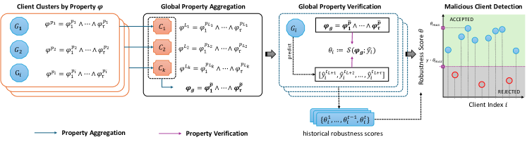
Figure 2: Overview of FLORAL. For each training round, FLORAL first conducts local logic inference to acquire the local reasoning properties; which are then used as criterion to cluster clients. Global property $\varphi_{g}$ is calculated by aggregation of clustered properties. Using $\varphi_{g}$, the server $\mathcal{S}$ verifies the satisfaction scores $\theta$ for each clients and use them to determine the suspicious updates to be removed from final aggregation.

IV-A Local Logic Inference

We employ stochastic gradient descent (SGD) [3] as the optimization algorithm to update the neural network models (line 4, Algorithm 1), where $\eta$ denotes the learning rate for the gradient descent. The SGD update rule can be substituted with any other gradient descent-based algorithm.

$$G^{t}_{i}\leftarrow\operatorname{SGD}\left(G^{t},D_{i},\eta\right)$$ (2)

After each local training process is completed using Equation 2, each client $C_{i}$ will conduct a local logic inference to acquire their logic property and submit them to the server. Given a local model of client $C_{i}$ at round $t$, i.e., $G_{i}^{t}$, and $\mathcal{D}_{v}$ be a small sample of centralized server data. During each clustering process, our method generates the logic property $\varphi(p^{i})$ for each participating client based on their prediction $\mathcal{Y}^{t}_{i}$ on this set. Our method uses Equation 1 to infer a logic reasoning property $\varphi$ from the client prediction. Recall that any locally inferred logic reasoning property must be satisfied by every data point in the client dataset. Moreover, any STL formula can be represented by its equivalent Disjunctive Normal Form (DNF), which typically has the form of $P\vee Q\vee R\vee\ldots$. Each clause within a DNF formula consists of variables, literals, or conjunctions (e.g., $P:=p_{1}\wedge\neg p_{2}\wedge\ldots\wedge p_{n}$). Essentially, the DNF form defines a range of satisfaction where any clause connected with the disjunction operator satisfies the STL formula $\varphi$. After this step, each client $C_{i}$ has a logical property represented $\varphi(p^{i}):=\varphi_{1}(p^{i})\wedge\varphi_{2}(p^{i})\wedge\ldots\wedge\varphi_{n}(p^{i})$ extracted by logic inference.

IV-B Global Logic Inference

Given a set of local logic properties $\mathcal{P}=\{\varphi(p^{1}),\varphi(p^{2}),\ldots,\varphi(p^{m})\}$ at the $t^{th}$ round, the server aggregates them to construct the global property $P_{g}$ that all clients should satisfy. The core idea is to group clients with similar properties and derive a global property from these clusters. This approach helps mitigate both targeted and untargeted attacks, as malicious clients with properties considerably different from benign ones can be isolated, reducing their impact on the aggregated property $P_{g}$.

To categorize samples based on their styles, we use FINCH [56], a hierarchical clustering method that identifies groupings in the data based on neighborhood relationships, without requiring hyperparameters or predefined thresholds. FINCH is particularly suitable for scenarios with an uncertain number of clusters, making it ideal for clustering client properties. Mathematically, given a set of features $\mathcal{F}$, FINCH provides a set of partitions $\mathcal{L}=\{\Gamma_{1},\Gamma_{2},\cdots,\Gamma_{L}\}$, where each partition $\Gamma_{i}=\{C_{1},C_{2},\cdots,C_{\Gamma_{i}}\mid C_{\Gamma_{i}}>C_{\Gamma_{i+1}}\forall i\in\mathcal{L}\}$ represents a valid clustering of $\mathcal{F}$, with $\Gamma_{L}$ having the smallest number of classes. Using FINCH, we group clients based on their local properties $\{P_{i}\}$ as follows:

$$\mathcal{P}\xrightarrow{\text{FINCH}}\Gamma_{L_{k}}=\{C_{i}\}_{i=1}^{K}\wedge r_{i,k}\in\mathbb{R}^{m*K}$$ (3)

Here, $\{C_{i}\}_{i=1}^{K}$ is a set of clusters and $\mathbf{r}$ is the cluster assignment metric, where $r_{i,k}\in\mathbb{R}^{m*K}$ and $r_{i,k}=1$ if $i\in k$ else $r_{i,k}=0$. This technique implicitly clusters clients with similar logical properties, as properties from different domains are less likely to be adjacent. A key advantage of the FLORAL framework is its dynamic assignment of client models to clusters, allowing the aggregation process to adapt to changes in logic properties over time. Clients with similar temporal reasoning properties are grouped, while those with differing properties are not combined. Next, we will discuss how to extract cluster property for each cluster $C_{i}$.

Cluster Property Inference. For a given cluster $C_{i}=\{\varphi(p^{j})|\ \forall j\in[1,m]\wedge r^{j,i}=1\}$, where local property $\varphi(p^{j})$ is from client $j^{th}$ in cluster $C_{i}$, the corresponding cluster property $P_{L_{i}}$ is computed as:

$$P_{L_{i}}:=\varphi(\bar{p}),\quad\bar{p}:=\frac{1}{|C_{i}|}\sum_{j=1}^{|C_{i}|}p_{j}$$ (4)

In Equation 4, $\bar{p}$ represents the average of the properties inferred by the local clients within the cluster, and $P_{L_{i}}$ denotes the cluster property expressed in the same STL (Signal Temporal Logic) syntax as the local models. The rationale behind this approach is to derive a representative property for the cluster by aggregating the individual properties of the clients. By averaging the properties, we create a cluster property that captures the commonalities among clients in the cluster, thus providing a robust and collective representation of their logic properties.

Global Property Inference. Given a set of cluster properties $\{P_{L_{i}}=\varphi(p^{L_{i}})|\forall i\in[1,K]\}$, the global property is then calculated as the median of these parameters from cluster properties.

$$P_{g}:=\varphi(\tilde{p}),\quad\tilde{p}:=Med(p^{L_{i}}),\forall i\in[1,K],$$ (5)

The idea of using clustered clients is popular in the context of heterogeneous data and non-IID (non-independent and identically distributed), where the local properties may vary widely. Motivated by this, we construct the global property by treating each cluster property equally instead of each local property. This helps the global property to reflect the properties of that group’s data better, which results in better model generalization within each group and avoids a one-size-fits-all property that may not suit clients with vastly different data distributions. Since median use is less sensitive to extreme values or outliers, we can minimize the influence of adversarial clients, whose properties deviate significantly from the benign ones. This aggregation process aligns to build a global model that is resilient to both targeted and untargeted attacks, as it reduces the impact of malicious clients whose properties deviate significantly from the benign ones.

IV-C Global Property Verification

Given a global property $\varphi(\tilde{p})$, this component assesses the level of satisfaction for each percentage of network predictions, denoted by $\hat{\mathcal{Y}}=(y_{L+1},\ldots,y_{L+\tau})$, with respect to a specified property $\varphi$. The property $\varphi$ is induced by the input sequence $\mathcal{X}=(x_{1},\ldots,x_{L})$, and its satisfaction level indicates how well the predicted sequence $\hat{\mathcal{Y}}$ for the next $\tau$ time-steps adheres to the property when conditioned on the input sequence $\mathcal{X}$. This framework enables us to quantify the degree to which the network’s predictions align with the desired property. We formalize the concept of a robustness score $\theta$ in Definition 4.

Definition 4 (Robustness Score $\theta$).

Given a network’s prediction $\hat{\mathcal{Y}}=\left(y_{L+1},\ldots,y_{L+\tau}\right)$, logical property $\varphi$ and scoring function $\mathcal{S}$, robustness score $\theta$ quantify the degree to which the predicted sequence $\hat{\mathcal{Y}}$ adheres to the specified property $\varphi$. Formally,

$$\theta:=\mathcal{S}(\varphi,\hat{\mathcal{Y}})=\{\rho(\varphi,\mathcal{Y},t)|\ \forall t\in[L+1,L+\tau]\},$$ (6)

where $\rho(\varphi,x,t)$ maps an STL formula $\varphi$, a signal trace $\mathcal{Y}$ at time $t$, to a value.

Depending on the selection for the scoring function, for each property, $\rho$ can return a binary value of satisfaction status or return a real value for the satisfaction level [32, 20]. We provide a practical example of STL property verification in Example 2.

Example 2 (Example of STL verification).

Given the STL property $\varphi=\square_{[0,5)}((x_{1}\geq 0.2)$ $\wedge$ $(x_{1}\leq 2.5)$ $\wedge$ $(x_{2}\geq 6)\wedge(x_{2}\leq 10))$, we evaluated the robustness score $\theta$ using predicted sequences $\hat{\mathcal{Y}}$ = $[(0.4,4),(0.45,5),(0.55,6),(0.75,7),(1.0,9)]$. The scoring function $\rho(\varphi,\mathcal{Y},t)$ calculates the degree of satisfaction at each time step by checking if both $x_{1}$ and $x_{2}$ lie within their specified bounds and returns a boolean value. The final score $\theta$ is $[\bot,\bot,\top,\top,\top,\top]$.

For each training round, after the robustness score is calculated using Definition 4, the server collects a set of scores for each client, denoted as $\theta^{t}:=\{\theta_{1}^{t},\theta_{2}^{t},\ldots,\theta^{K}_{t}\}$. To convert the robustness score $\theta$ from qualitative semantics (i.e., boolean values) to numerical values, we compute the percentage of the ’True’ signal predicate, denoted by $\top$. Using this verification score helps assess the trustworthiness of each client because the global property $\varphi$ represents the collective standards and requirements derived from all clients in the system. Therefore, higher scores $\theta$ indicate that a client’s predictions align well with these global properties or at least with the majority of benign clients, suggesting that the client’s model is reliable and trustworthy, i.e., more likely to be a benign client. Conversely, lower scores $\theta$ may reveal discrepancies or issues with the client’s model or data, potentially indicating anomalies or malicious behavior, and thus warrant further investigation. Clients whose predictions do not satisfy the global property may cause significant deviations from the global objective and the predictions of benign clients, thereby affecting the overall model performance and reliability. Over time, benign clients will increasingly agree on the training objective, leading their models to become more similar and showing higher alignment in their predictions when given the same dataset. As a result, these benign clients should have higher verification scores $\theta$, reflecting their consistent adherence to the global property and reinforcing their trustworthiness.

For each training round, after verification, the server collects a set of robustness scores for each client, denoted as $\theta^{t}:=\{\theta_{1}^{t},\theta_{2}^{t},\ldots,\theta_{K}^{t}\}$. These scores are used to detect malicious clients. The intuition is that benign local models align with the global model objective and share the same learning goals, while malicious models often distort the global model’s behavior, leading to discrepancies in their predictions. Consequently, a higher robustness score indicates greater trustworthiness. Detecting and excluding updates from malicious clients is crucial to prevent the global model from being poisoned. To further strengthen the reliability of the robustness score, historical information is used to update scores cumulatively. Specifically, the score for client $i$ is updated as follows:

$$\theta_{i}=\frac{f_{i}-1}{f_{i}}\theta_{i}+\frac{1}{f_{i}}\theta_{i}^{t},$$ (7)

where $\theta_{i}$ is the cumulative score, $\theta_{i}^{t}$ is the current round’s score, and $f_{i}$ represents the number of training rounds client $i$ has participated in up to round $t$. Using historical data to update the robustness scores is beneficial because it smooths out fluctuations in individual scores that might occur due to temporary anomalies or noise in specific rounds. By incorporating cumulative scores, the method accounts for the overall consistency and performance of each client over multiple rounds, rather than relying solely on potentially erratic single-round evaluations. This approach helps in identifying clients that consistently adhere to the global property, thereby improving the robustness and reliability of the client assessment process and reducing the impact of transient malicious behavior.

IV-D Malicious Client Detection

To identify and filter out malicious clients, we use a binary mask $\mathcal{M}\in\mathbb{R}^{m}$, where each element $\mathcal{M}_{i}$ indicates whether a client $i$ is considered malicious. The mask is defined as follows:

$$\mathcal{M}_{i}=\begin{cases}1&\text{if }\theta_{i}\geq\gamma\cdot\max{(\theta_{j})},\\ 0&\text{otherwise}.\end{cases}$$ (8)

Here, $\gamma$ is a threshold parameter that determines the cutoff for filtering out malicious models. Note that the trustworthy scores $\theta$ are normalized before applying Equation 8. The rationale behind this approach is that models producing predictions with significantly lower robustness scores are more likely to be compromised or adversarial, especially if they are in the minority. The assumption is that the properties of poisoned models, which are often outliers or deviate from the global property, will exhibit lower scores compared to the majority of benign clients. The robustness threshold for each training round is determined based on the distribution of the robustness scores across all clients. This threshold helps in distinguishing between reliable and unreliable client updates.

To ensure the integrity of the global model, only updates from non-malicious clients are used for aggregation. The global model $\boldsymbol{w}_{t}$ at round $t$ is updated as follows:

$$\boldsymbol{G}_{t}=\mathcal{A}(\boldsymbol{G}_{t-1};\{\nabla_{i}\mid\forall i\in[1,m]\text{ and }\mathcal{M}_{i}=1\}),$$ (9)

where $\mathcal{A}$ represents the aggregation function used by the server to combine the updates from the selected non-malicious clients. In this formulation, $\nabla_{i}$ denotes the model update from client $i$. By excluding updates from clients marked as malicious (i.e., those with $\mathcal{M}_{i}=0$), the server can ensure that the global model $\boldsymbol{w}_{t}$ is not adversely affected by compromised or unreliable client contributions. This method enhances the robustness of the global model and helps maintain its performance by focusing on contributions from trustworthy clients.

Input :  $G_{0},T,N,K$ $\quad\triangleright$ $G_{0}$ is the initial global model, $T$ is total training round, $N$ is total clients and $K$ is total participating clients for a training round;

$n_{i},\forall i\in N$ $\quad\triangleright$ Size of local training data;

$D_{v}$: global validation set;

Output :  $G^{T}$: $\quad\triangleright$ The updated global model after $T$ training iterations

1

2for iteration $t$ in $[1,\ldots,T]$ do

3       Server samples a subset $\mathcal{C}_{t}=\{C_{1},C_{2},\ldots,C_{i},\ldots,C_{m}\}$ of $m$ clients per total $N$ clients randomly;

4       for each client $i$ in $\mathcal{C}_{t}$ do

5             $G^{t}_{i}\leftarrow\operatorname{SGD}\left(G^{t},D_{i},\eta\right)$ $\quad\triangleright$ local model update;

6             Generate $\hat{\mathcal{Y}_{i}}$ with $G^{t}_{i}$ and $\mathcal{D}_{v}$;

7             Generate client logic property $\varphi(p^{i})$ on prediction $\hat{\mathcal{Y}_{i}}$;

8       end for

9      $\mathcal{P}=\{\varphi(p^{1}),\varphi(p^{2}),\ldots,\varphi(p^{m})\}$;

10      

11      $\mathcal{P}\xrightarrow{\text{FINCH}}\Gamma_{L_{k}}=\{C_{i}\}_{i=1}^{K}\wedge r_{i,k}\in\mathbb{R}^{m*K}$;

12      

13      for each cluster $C_{i}$ in $\Gamma_{L_{k}}$ do

14             $P_{L_{i}}:=\varphi(\bar{p}),\quad\bar{p}:=\frac{1}{|C_{i}|}\sum_{j=1}^{|C_{i}|}p_{j}$

15       end for

16      $P_{g}:=\varphi(\tilde{p}),\quad\tilde{p}:=Med(p^{L_{i}})\forall i\in[1,K]$ $\ \triangleright$ global property;

17      

18      $\theta^{t}:=\{S(\varphi(\tilde{p});\mathcal{Y}_{i})|\forall i\in[1;m]\}$ $\ \triangleright$ calculate robustness score;

19       Update historical $\theta$ using Eqn. 7;

20       Update malicious mask $\mathcal{M}$ using Eqn. 8;

21       $G^{t}=\mathcal{A}\left(G^{t-1};\left\{G^{t}_{i}\mid\forall i\in[1,m]\text{ and }\mathcal{M}_{i}=1\right\}\right)$;

22 end for

23

return $G_{T}$

Algorithm 1 FLORAL

V Experiments

In this section, we evaluate the performance of FLORAL against various poisoning attack scenarios, including untargeted and targeted attacks. We show that FLORAL outperforms state-of-the-art FL defenses including Krum/Multi-krum [9], FoolsGold [17], RFA [50], RLR [47], FLAME [42], and FLDetector [73] in mitigating these attacks. We used an Amazon EC2 g5.4xlarge instance for all experiments, equipped with one NVIDIA A10G Tensor Core GPU, 16 vCPUs, 64 GB of memory, and 24 GB of dedicated GPU memory.

V-A Experiment Setup

In this subsection, we first describe the datasets and models used in this work, followed by details on the attack settings, baselines, evaluation metrics, and FL simulation.

Datasets. In this work, we conducted experiments using two time-series datasets which are LTE Physical Downlink Control Channel (PDCCH) measurements [48] and Federal Highway Administration [16]. The PDCCH dataset was collected from three different base stations in Barcelona, Spain, which is publicly accessed by Perifanis et al. [48]. We further separate data from these three stations into 30 sub-clients to simulate the FL environment. 11 features related to downlink and uplink traffic are provided for each site. Following the settings by Perifanis et al. [48], the objective is to predict the first five measurements for the next timestep using as input the observations with a window of size $\tau=10$ per base station. This is considered a multi-variate time series regression task. The FHWA dataset is a real-world dataset of highway traffic data. We obtained a publicly available dataset from the Federal Highway Administration (FHWA 2016) and preprocessed hourly traffic volume from multiple states. After preprocessing and excluding low-quality and missing data, we continue with the final data from 15 states, this setting is followed [3]. Further, we design a testing scenario where a neural network is trained to predict the traffic volume for the next $\tau=24$ consecutive hours based on the past traffic volume at a location over the previous five days. This is considered a univariate time series regression task. In both datasets, we specifically focus on the operational range property, as outlined in Table I, which captures important aspects of the traffic volume dynamics for each client during two-hour windows. For these two datasets, we focus on using Operational Range (Table I) for logic reasoning inference and qualitative semantics for verification.

Attack settings. We evaluate different defenses under both untargeted attacks and targeted attacks.

Regarding untargeted attacks, we consider Gaussian Byzantine attack followed by Fang et al. [15], where for a byzantine client $i$ in iteration $r$, the message to be uploaded is set to follow a Gaussian distribution, i.e., $\nabla_{i}^{t}\sim\mathcal{N}\left(0,\sigma_{\mathrm{G}}^{2}\right)$. This attack randomly crafts local models, which can mimic certain real-world scenarios where compromised devices might produce erratic or unexpected updates.

Regarding targeted attacks, we consider the case where malicious clients use a flip attack to manipulate the training data, i.e., data poisoning. Specifically, the adversary aims to disrupt a machine learning model by modifying a subset of data points to their extreme target values [38]. This attack is conducted by computing the distance of each target value $\mathcal{Y}_{t}\in\mathcal{Y}$ from the nearest boundary (i.e., $\mathcal{Y}_{min},\mathcal{Y}_{max}$) of the feasibility domain, then selecting the points with the largest distances and flipping their target values to the opposite extremes. Under this attack, the victim model shifts the target variable to the other side’s extreme value of the feasibility domain. In FL, to make poisoning attacks stronger and more stealthy against defenses, adversaries often combine data poisoning (as discussed above) with model poisoning techniques [44, 6]. We consider three such model poisoning techniques: Constrain-and-scale, Projected Gradient Descent (PGD), and Model Replacement attacks [6, 44], which are combined with data poisoning to strengthen the poisoning effect. Consequently, when evaluating targeted attacks, we examine four strategies: (i) Targeted Attack (without model poisoning), (ii) PGD Attack (Targeted Attack combined with PGD), (iii) Constrain-and-Scale Attack (Targeted Attack combined with Constrain-and-Scale), and (iv) Model Replacement Attack (Targeted Attack combined with Model Replacement).

Defense baselines. We implement seven representative FL defenses for byzantine attacks and targeted attacks including Krum/Multi-Krum [9], RFA [50], Foolsgold [17], FLAME [42], RLR [47], and FLDectector [73]. We provide detailed parameter settings in the Appendix.

Evaluation metrics. We evaluate the model performance using the Mean Absolute Error (MAE) and Mean Squared Error (MSE). MAE measures the absolute difference between the expected and predicted output. MSE measures how far predictions are from the ground truth values using the Euclidean distance. The considered metrics are defined as follows: $\text{MSE}=\frac{1}{n}\sum_{i=1}^{n}(y_{i}-\hat{y}_{i})^{2}$; and $\text{MAE}=\frac{1}{n}\sum_{i=1}^{n}|y_{i}-\hat{y}_{i}|$.

Simulation setting. We simulate an FL system with a total of $N$ clients; in each training round, the server randomly selects $k\%$ of clients to participate, a process known as client sampling. Unless otherwise specified, $N$ is set to 30 and 100 for the PDCCH and FHWA datasets, respectively, with $k$ fixed at 50%. The number of communication rounds is set to 20 for both datasets, with 3 local training epochs per round. For all experiments and algorithms, we use SGD with consistent learning rates and a batch size of 128. A vanilla RNN model is employed as the backbone network. More details can be found in our Appendix.

V-B Results

First, we report the robustness of the different defenses against both untargeted and targeted attacks in terms of MSE and MAE in Section V-B1 and Section V-B2. Following this, we compare our method against baselines under varied adversarial power, represented by their attack ratio, in Section V-B3 . Lastly, we evaluate the stability of our method across different system and attack settings by varying two important factors in FL [45, 42], namely (i) the FL aggregator and (ii) the model architecture, as discussed in Section V-B4.

V-B1 Robustness on Untargeted Attack

TABLE II: Defense efficacy under Byzantine Attacks with FHWA and PDCCH datasets.

	PDCCH Dataset				FHWA Dataset
Methods	Full		Partial		Full		Partial
	MSE	MAE	MSE	MAE	MSE	MAE	MSE	MAE
Krum	.0066	.0455	.0066	.0478	.0139	.0741	.0107	.0661
Multi-Krum	.8706	.7428	.0105	.0910	.5991	.6316	6.326	2.062
RFA	.0053	.0389	.0071	.0694	.0027	.0338	.0052	.0495
FoolsGold	.0591	.1650	.0575	.2912	.7358	.7491	.4878	.6096
FLAME	.0047	.0387	.0058	.0563	.0134	.0703	.0133	.0712
RLR	33.21	5.545	.0111	.0652	.3283	.4439	1.488	.9757
FLDetector	.0168	.0944	.0078	.0750	.3959	.4986	.0295	.1159
Ours	.0045	.0378	.0045	.0376	.0021	.0351	.0011	.0227

TABLE III: Defense efficacy under Targeted Attacks with different model poisoning techniques under the PDCCH dataset.

Methods	Targeted		PGD		Constrain-and-scale		Model Replacement
	MSE	MAE	MSE	MAE	MSE	MAE	MSE	MAE
Krum	.0066	.0478	.0066	.0478	.0107	.0854	.0066	.0472
Multi-Krum	.0105	.0910	.0105	.0910	.0058	.0550	.0105	.0909
RFA	.0071	.0694	.0071	.0694	.0059	.0581	.0072	.0695
FoolsGold	.0575	.2091	.0575	.2091	.0521	.2155	.0568	.0564
FLAME	.0058	.0563	.0058	.0563	.0053	.0482	.0058	.0563
RLR	.0111	.0652	.0111	.0652	.0069	.0466	.0061	.0456
FLDetector	.0078	.0750	.0078	.0750	.0048	.0460	.0080	.0783
Ours	.0046	.0380	.0046	.0380	.0046	.0385	.0046	.0380

TABLE IV: Defense efficacy under Targeted Attacks with different model poisoning techniques under the FHWA dataset.

Methods	Targeted		PGD		Constrain-and-scale		Model Replacement
	MSE	MAE	MSE	MAE	MSE	MAE	MSE	MAE
Krum	.0257	.1021	.0257	.1021	.0049	.0475	.0226	.0882
Multi-Krum	.0279	.1377	.0279	.1377	1.001	.9080	.0287	.1396
RFA	.0126	.0823	.0135	.0874	.0135	.0874	.0124	.0805
FoolsGold	.1333	.5459	.1333	.2960	2.394	1.368	.1003	.2576
FLAME	.0297	.1221	.0297	.1221	.0358	.1397	.0297	.1221
RLR	.0254	.1154	.0254	.1154	1.325	1.032	.0260	.1214
FLDetector	.0233	.1239	.0233	.1239	.0194	.0971	.0395	.1647
Ours	.0014	.0318	.0014	.0318	.0012	.0261	.0014	.0318

We first evaluate our method against Byzantine attacks and then compare it with the state-of-the-art defenses for both full and partial scenarios. In a full scenario, all clients participate in the training while in the partial scenario, the server $\mathcal{S}$ randomly selects $m$ clients to participate in the training each round. We show the results in Table II and highlight the best in bold. As presented, most defenses failed to mitigate the effect of malicious clients. The performance results show that our method achieves the best results in both full and partial data scenarios across the PDCCH and FHWA datasets. In contrast, methods like Multi-Krum and RLR show considerable performance degradation, especially in the FHWA dataset. Multi-Krum, for example, has an MSE increase from 0.5991 to 6.326 when faced with full and partial cases, signaling instability when faced with less data. The explanation for this phenomenon is that in the FHWA dataset, the data itself reflects a higher degree of heterogeneity and each client owns a smaller fraction of data from the virtual global data, which is considered as a more challenging scenario. RLR, similarly, exhibits extreme variability with very high error rates in the full dataset and moderate ones in the partial dataset. This suggests that such methods may not be suitable for scenarios where data availability fluctuates. Notably, methods like Krum, RFA, and FLAME perform reasonably well compared to remaining baselines, particularly in the full data setting, though they show degradation in partial data cases. Moreover, the performance of these methods across different datasets is unstable. FLDetector and FoolsGold, meanwhile, demonstrate mixed results, with FoolsGold showing particularly high errors on the FHWA dataset, indicating potential weaknesses in handling the specific characteristics of this dataset. Overall, our method demonstrates superior generalization, maintaining robust performance while other methods show variability or degradation, especially when data observation is incomplete — i.e., only a portion of clients participate each round.

V-B2 Robustness on Targeted Attack

In addition to the attacks mentioned in Table II, we demonstrate the effectiveness of our method under more types of targeted attacks in Table III and Table IV. The tables highlight the performance of various federated learning defense methods against different attacks: Targeted, PGD, Constrain-and-scale, and Model Replacement. Across all attack types, our method consistently outperforms the others, achieving the lowest MSE and MAE values. For instance, against the targeted attack, our method records an MSE of 0.0046 and 0.0014 for PDCCH and FHWA datasets while the second-best baseline numbers are 0.0058 and 0.0297, respectively. Therefore, our method outperforms the second-best baseline by 20.69% on the PDCCH dataset and by 93.27% on the FHWA dataset in terms of MSE. Methods like FLAME and RFA perform better across considered baselines with different attack methods and datasets. However, these methods produce unstable performance in different settings. FLAME, for example, performs relatively well with the PDCCH dataset but it fails to mitigate the poisoning attacks with the FHWA dataset, resulting in higher errors compared to other baselines. The reason is that FHWA demonstrates a much higher degree of heterogeneity, so the updates from even benign clients may experience large deviations. Therefore, using solely pairwise distance-based similarities to detect malicious clients may be ineffective. This phenomenon is consistent among other defenses such as FLDetector, Multi-Krum, and RLR.

In addition, when the adversary combines the data poisoning attack with various model poisoning techniques, the defenses encounter difficulty and show mixed results. Indeed, in the PDCCH dataset, RLR can mitigate the constrain-and-scale attack but encounter remarkably higher errors with targeted and PGD attacks. At the same time, FLDectector can handle constrain-and-scale attacks better than PGD and model replacement attacks. We conclude that existing baselines struggle to maintain low error rates across all various attack settings. Moreover, using additional model poisoning techniques introduces more challenges to existing defenses because most model-centric defense approaches like Multi-Krum rely on specific metrics to distinguish between benign and malicious gradients, e.g., Euclidean and cosine distance, which are susceptible to metric-constrained attacks. Meanwhile, our method consistently achieves the lowest MSE and MAE values across all scenarios, demonstrating superior robustness and adaptability to various complicated attack strategies.

V-B3 Effect of Different Attack Ratios

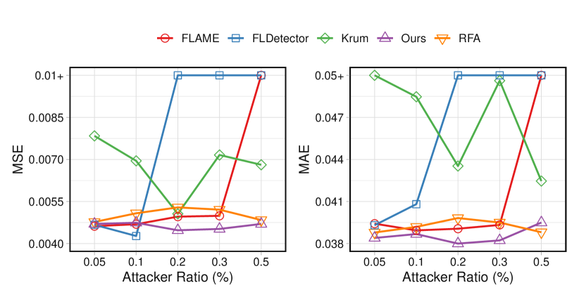
(a) PDCCH Dataset.

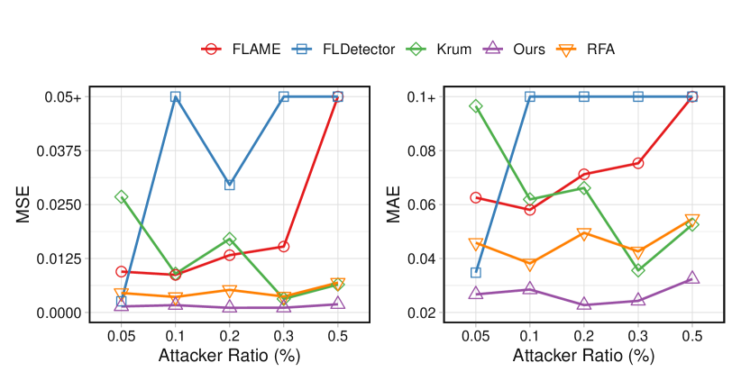
(b) FHWA Dataset.

Figure 3: Zoom-in analysis of our method’s robustness against Byzantine Attacks, compared to various defense mechanisms under different attack ratios $\epsilon$.

TABLE V: Comparing performance of different defenses under various attack ratios $\epsilon$.

	Methods	0.05		0.1		0.2		0.3		0.5
		MSE	MAE	MSE	MAE	MSE	MAE	MSE	MAE	MSE	MAE
PDCCH Dataset	Krum	.0078	.0505	.0070	.0485	.0051	.0435	.0072	.0496	.0068	.0425
	Multi-Krum	.0044	.0379	.2987	.3869	.7665	.7005	1.178	.8686	7.643	2.181
	RFA	.0048	.0388	.0051	.0392	.0053	.0398	.0052	.0395	.0048	.0388
	FoolsGold	.0076	.0492	.0080	.0605	.0765	.1950	.0551	.1594	.0424	.1394
	FLAME	.0046	.0394	.0047	.0389	.0050	.0391	.0050	.0393	.0780	.2025
	RLR	.0978	.2679	2.011	1.117	2.515	1.403	2.456	1.367	39.88	5.820
	FLDetector	.0047	.0393	.0043	.0408	1.862	1.170	1.788	1.156	10.97	2.650
	Ours	.0047	.0384	.0047	.0387	.0045	.0376	.0045	.0382	.0047	.0395
FHWA Dataset	Krum	.0268	.0965	.0090	.0619	.0170	.0661	.0031	.0356	.0065	.0526
	Multi-Krum	.1347	.2897	1.277	.8875	6.326	.0622	7.730	2.227	18.05	3.321
	RFA	.0045	.0458	.0036	.0382	.0052	.0495	.0037	.0426	.0069	.0547
	FoolsGold	.0746	.2304	.3137	.4797	.4878	.6096	.6487	.7124	.9113	.8498
	FLAME	.0095	.0626	.0087	.0580	.0133	.0712	.0153	.0753	5.844	1.969
	RLR	.1820	.3551	1.328	.9699	1.488	.9757	7.001	2.096	3.689	1.562
	FLDetector	.0026	.0347	.0930	.2117	.0295	.1159	.0612	.1813	9.460	2.426
	Ours	.0014	.0267	.0017	.0285	.0011	.0227	.0011	.0243	.0019	.0324

We demonstrate the efficacy of different defenses against the various backdoor attacks under varying attack ratios $\epsilon$ in Figure 3 and Table V, where we compare our methods with other baselines with PDCCH and FHWA datasets. The attack ratio $\epsilon$ is sampled iteratively from $[0.05,0.1,0.2,0.3,0.5]$. As this ratio increases, it causes a more challenging scenario for the defenses due to the decreased benign ratio over malicious ones. The case of 0.5 is the most difficult one since the benign clients are now equal to the malicious ones. The result in Table V of the effect of attack ratio on the performance of different methods reveals significant variations in their robustness. When the attack ratio is 0.5, the performance of most methods deteriorates, but the extent of this degradation varies widely. For instance, FLORAL consistently shows the lowest MSE and MAE across all attack ratios, with notable improvements in error metrics as the attack ratio increases. Specifically, at a 0.5 attack ratio, FLORAL achieves the lowest MSE and MAE errors, demonstrating superior resilience compared to other methods.

In contrast, methods such as Multi-Krum and FoolsGold experience severe performance degradation as the attack ratios increase. For instance, Multi-Krum shows MSE values that escalate more than 100 times when $\epsilon$ rises from 0.05 to 0.5. Similarly, FoolsGold shows its vulnerability to higher attack ratios, i.e., errors increase linearly regarding the increase of attack ratio in FHWA datasets. RLR and FLDetector also exhibit varied impacts, with RLR showing notable error increases at higher ratios. While RFA and FLAME demonstrate their better stability with moderate performance reductions as the attack ratio increases, these two methods cannot beat the performance of FLORAL in all considered scenarios. Overall, FLORAL proves more robust and consistent across attack ratios, making it a reliable choice in high-attack scenarios. Other methods perform better at lower ratios but decline as attacks intensify, highlighting the need for robustness in adversarial settings.

V-B4 Generalization to System Settings

Effect of Different FL Aggregators.

TABLE VI: Defense efficacy of our method when combined with different aggregators.

Methods	Byzantine		Targeted
	MSE	MAE	MSE	MAE
FedAvg	6.701	2.088	.0341	.1528
FedAvg+	.0011	.0227	.0014	.0318
FedProx	8.226	2.318	.0241	.1341
FedProx+	.0027	.0457	.0027	.0463
Scaffold	.1765	1.757	.1594	.3536
Scaffold+	.0128	.0790	.0103	.0692
FedDyn	.0500	.1608	.0283	.1450
FedDyn+	.0014	.0301	.0013	.0278
FedNova	6.532	2.073	.0342	.1528
FedNova+	.0010	.0230	.0014	.0031

In this experiment, we evaluate the performance and stability of various FL aggregators under Byzantine and targeted attacks. The objective is to assess whether combining FLORAL with these aggregators can improve the robustness of the FL system. We select five aggregators including FedAvg, FedProx [28], Scaffold [24], FedDyn [1], FedNova [65], and denote their FLORAL-enhanced versions as FedAvg+, FedProx+, Scaffold+, FedDyn+, FedNova+. The result is presented in Table VI.

The results reveal a sustainable contrast in performance between baseline methods and their corresponding FLORAL-enhanced versions. Baseline methods, such as FedAvg and FedProx, exhibit substantial vulnerabilities to both Byzantine and Targeted attacks, as evidenced by their high Mean Squared Error (MSE) and Mean Absolute Error (MAE) values. For instance, FedAvg records an MSE of 6.701 and 0.0341 under Byzantine and Targeted attacks, respectively, indicating errors that are 6000 and 24 times higher compared to the defense case. Similarly, other aggregators also exhibit high error rates in both scenarios. In contrast, the enhanced methods demonstrate significantly improved performance. For example, FedAvg+ reduces the error in MSE by 99.98% compared to the original FedAvg version. The corresponding improvements for FLORAL with other methods are 99.97% for FedProx, 92.75% for Scaffold, 97.20% for FedDyn, and 99.98% for FedNova. Under targeted attacks, FLORAL also proves effective, reducing error caused by malicious clients of up to 99.41% for MSE and 80.46% for the MAE metric. Results in Table VI show that using data heterogeneity-tailored aggregators can affect the poisoning attacks and defenses in FL, suggesting an interesting research direction. Overall, the result highlights the effectiveness of incorporating FLORAL into various FL aggregators against different types of poisoning attacks.

Effect of Different Model Architectures.

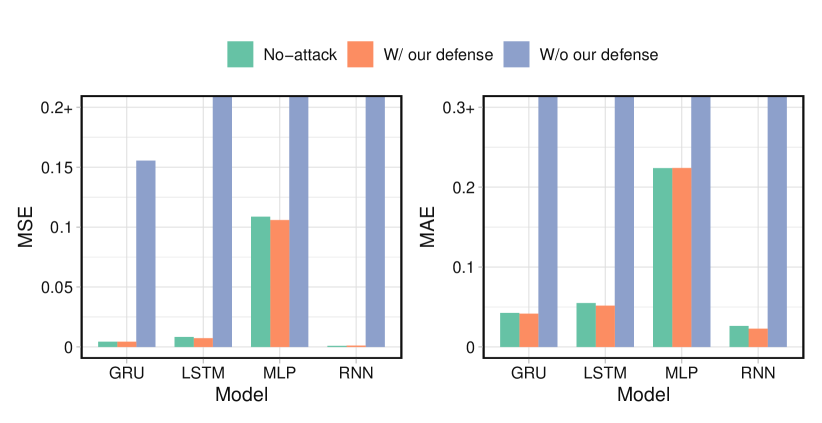
(a) Byzantine Attacks

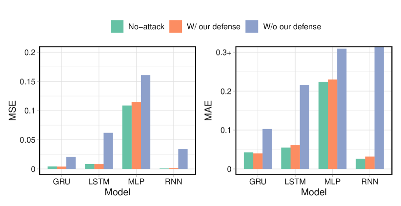
(b) Targeted Attacks

Figure 4: Zoom-in robustness of our method when applied with different model architectures.

In this experiment, we assessed different model architectures to verify the applicability of our method across various settings. We evaluated three versions for each architecture: the vanilla model (no attack), the poisoned model (attack without defense), and the defended model (attack with defense FLORAL applied) and presented the results in Figure 4. Under the Byzantine attack, the aggregating poisoning updates from malicious clients degrade model performance drastically, i.e., resulting in at least 20 times higher errors. In contrast, adding FLORAL substantially mitigates poisoning effects caused by malicious clients, thus reducing MSE and MAE by over 99.6% and 93.3%, respectively. Moreover, using FLORAL helps to achieve low errors comparable to the vanilla models. This observation is consistent across different model architectures including LSTM, GRU, MLP, and RNN.

In the Targeted attack scenario, FLORAL also shows its efficacy with different model architectures. Indeed, while the poisoned model exhibits performance degradation, using FLORAL with LSTM backbone reduces the MSE from 0.06 to 0.02 (a 66.7% improvement) and the MAE from 0.22 to 0.09 (a 59.1% improvement). In all model architectures, FLORAL consistently mitigates the effect of poisoning attacks as close to the one of a vanilla model. To this end, FLORAL can mitigate both untargeted and targeted attacks and provide robust performance improvements across various architectures.

VI Conclusion

In this study, we address a critical gap in FL robustness by focusing on the specific challenges posed by poisoning attacks within the FTS domain. Mainstream FL defenses have primarily targeted computer vision applications, leaving time series data largely unexamined. Therefore, when applied in FTS, these defenses showcase their limited efficacy. We introduce FLORAL, a defense mechanism designed to tackle these challenges effectively. FLORAL leverages a unique approach that combines formal logic reasoning with hierarchical clustering to evaluate client trustworthiness and align predictions with global time-series patterns. This method diverges from traditional model-centric defenses by focusing on the logical consistency of client contributions, which enhances its ability to detect and mitigate adversarial behaviors. The results from our experiments on two distinct datasets and various attack settings demonstrate that FLORAL outperforms existing baseline methods, confirming its efficacy in improving the robustness of FL systems for time series applications. Future work could extend this approach to other types of time series data and explore its integration with other defense mechanisms to further bolster FL security.

This document serves as an extended exploration of our research, providing a detailed implementation and discussion of experiments provided in the main text. Appendix -A presents additional details on STL and the STL-based property inference and verification tasks. Appendix -B provides a comprehensive discussion of the training process, including datasets, model structures, and configurations used to reproduce the reported results. Additionally, we present supplementary results not included in the main paper in Appendix -C. Our code is available at https://anonymous.4open.science/r/FLORAL-Robust-FTS.

-A Signal Temporal Logic: Inference and Verification

To begin, we follow [3, 32] to present the qualitative (Boolean) semantics for an STL formula $\varphi$. Here, we use the following notations: $\mathbf{x}$ denotes a signal trace, $\mu$ denotes an STL predicate, and $\varphi,\varphi_{1}$, and $\varphi_{2}$ represent different STL formulas.

Definition 5 (STL Qualitative Semantics).

$$\begin{array}[]{lll}(\mathbf{x},t)\vDash\top&\leftrightarrow&\top\\ (\mathbf{x},t)\vDash\mu&\leftrightarrow&\mu(\mathbf{x}[t])\\ (\mathbf{x},t)\vDash\varphi_{1}\vee\varphi_{2}&\leftrightarrow&(\mathbf{x},t)\vDash\varphi_{1}\vee(\mathbf{x},t)\vDash\varphi_{2}\\ (\mathbf{x},t)\vDash\varphi_{1}\wedge\varphi_{2}&\leftrightarrow&(\mathbf{x},t)\vDash\varphi_{1}\wedge(\mathbf{x},t)\vDash\varphi_{2}\\ (\mathbf{x},t)\vDash\Diamond_{[a,b]}\varphi&\leftrightarrow&\exists t^{\prime}\in[t+a,t+b],\left(\mathbf{x},t^{\prime}\right)\vDash\varphi\\ (\mathbf{x},t)\vDash\square_{[a,b]}\varphi&\leftrightarrow&\forall t^{\prime}\in[t+a,t+b],\left(\mathbf{x},t^{\prime}\right)\vDash\varphi\\ (\mathbf{x},t)\vDash\varphi_{1}\mathcal{U}_{[a,b]}\varphi_{2}&\leftrightarrow&\exists t^{\prime}\in[t+a,t+b],\left(\mathbf{x},t^{\prime}\right)\vDash\varphi_{2}\\ &&\wedge\forall t^{\prime\prime}\in\left[t,t^{\prime}\right],\left(\mathbf{x},t^{\prime\prime}\right)\vDash\varphi_{1}\end{array}$$

While the qualitative semantics in Def. 5 provide a Boolean evaluation of the satisfaction of an STL property, there are inference tasks that rely on a real-valued measurement of property satisfaction, known as the STL robustness metric $(\rho)$. Def. 6 below describes how this metric is calculated, which maps a given signal trace $\mathbf{x}$ and an STL formula $\varphi$ to a real number over a specified time interval $I$.

Definition 6 (STL Quantitative Semantics).

The robustness metric $\rho$ maps an STL formula $\varphi$, a signal trace $\mathbf{x}$, and a time $t$ to a real value such that:

$$\rho(\mathbf{x},\varphi,t) =g(\mathbf{x}(t))-\alpha\text{ where }\mu(X)\text{ is }g(X)\geq\alpha$$

$$\rho(\neg\varphi,\mathbf{x},t) =-\rho(\varphi,\mathbf{x},t)$$

$$\rho(\varphi_{1}\vee\varphi_{2},\mathbf{x},t) =\max\{\rho(\varphi_{1},\mathbf{x},t),\rho(\varphi_{2},\mathbf{x},t)\}$$

$$\rho(\varphi_{1}\land\varphi_{2},\mathbf{x},t) =\min\{\rho(\varphi_{1},\mathbf{x},t),\rho(\varphi_{2},\mathbf{x},t)\}$$

$$\rho(\Diamond_{I}\varphi,\mathbf{x},t) =\underset{t^{\prime}\in(t,t+I)}{\max}\rho(\varphi,\mathbf{x},t^{\prime})$$

$$\rho(\square_{I}\varphi,\mathbf{x},t) =\underset{t^{\prime}\in(t,t+I)}{\min}\rho(\varphi,\mathbf{x},t^{\prime})$$

$$\rho(\varphi_{1}\mathcal{U}\varphi_{2},\mathbf{x},t) =\sup_{t^{\prime}\in(t+I)\cap\mathbb{T}}(\min\{\rho(\varphi_{2},\mathbf{x},t^{\prime}),$$

$$\,\quad\inf_{t^{\prime\prime}\in[t,t^{\prime}]}(\rho(\varphi_{1},\mathbf{x},t^{\prime\prime}))\})$$

-B Training configurations

-B1 Baselines

• Krum/Multi-Krum [9]: Krum and Multi-Krum algorithms are Byzantine-resilient aggregation techniques designed for federated learning to defend against malicious or faulty clients during model training. These methods work by selecting the update(s) from a client(s) closest to most other clients’ updates, minimizing the impact of outliers or adversarial updates.

• RFA [50]: RFA replaces the weighted averaging mechanism by using the geometric median for aggregating model updates, protecting against data and model poisoning without revealing individual contributions.

• FoolsGold [17]: FoolsGold adjusts the learning rate for each client based on updated similarity and historical data. It uses cosine similarity to measure the angular distance between updates.

• FLAME [42]: FLAME is a backdoor defense that includes three components: DP-based noise injection to remove backdoor contributions, unsupervised model clustering to detect and eliminate poisoned updates, and weight clipping to limit the impact of malicious updates.

• RLR [47]: RLR proposes a lightweight defense against backdoor attacks in federated learning by adjusting the aggregation server’s learning rate per dimension and per round, based on the majority sign of agents’ updates.

• FLDetetor [73]: FLDetector identifies and removes malicious clients in federated learning by monitoring the consistency of their model updates. It predicts updates using the Cauchy mean value theorem and L-BFGS, flagging clients as malicious if their actual updates deviate from predictions over multiple iterations.

With the implementations of these baselines, most hyper-parameters are inherited with minor modifications. Several parameters are adjusted to make experiment settings more appropriate. Other hyperparameters without mention are set up as in the original works.

Robust threshold $\theta$ of RLR [47]. The value of $\theta$ in the RLR method is specified to be any value between [$m\cdot\epsilon+1$, $m-m\cdot\epsilon$], where $m$ is the number of participants each round and $\epsilon$ is the proportion of malicious clients, according to the authors. Because there is limited to one malicious client each round, the value of $\theta$ is set to $1$ throughout the experiments with all datasets.

Estimated number of Byzantine clients $F$ in Krum/Multi-Krum [9]. Since the experiments are conducted under fixed-pool backdoor attacks with a maximum of one malicious client, so $F$ is set to be $\max{(\lfloor\epsilon\cdot m\rfloor,1)}$.

Estimated number of Byzantine clients in FLDetector [73]. We set the number of byzantine clients as $\lfloor\epsilon\cdot m\rfloor$, corresponding to the potential number of malicious clients appearing in each training round.

-B2 Training hyper-parameters

We have a fixed number of 30/100 FL clients for PDCCH/FHWA in each testing scenario. During the communication rounds, 50% of the clients are randomly selected. The batch size is 128, and the test batch size is 256. We set the maximum learning rate for the MLP, RNN, LSTM, and GRU models to be 0.001. To optimize the models, we utilize the SGD optimizer in the PyTorch implementation. We use the mean squared error (MSE) loss, implemented in PyTorch, which is commonly employed in regression tasks. In our default setup, the number of local training epochs is set to 3 if not otherwise specified.

-B3 Different Aggregators.

• FedProx [28]: An extension of FedAvg that incorporates a proximal term to ensure that local models remain close to the global model, enabling better performance in non-IID settings and allowing for partial client participation.

• FedDyn [1]: Introduces a dynamic regularization technique for each device in Federated Learning to ensure alignment between local and global solutions over time. This approach improves training efficiency in both convex and non-convex settings while being robust to device heterogeneity, partial participation, and unbalanced data.

• Scaffold [24]: Aims to mitigate the drift between local and global models by using control variates, which stabilize client updates and enhance convergence, particularly in settings with high data heterogeneity

• FedNova [65]: Enhances the federated averaging process by considering the contribution of each client based on the number of samples they have, aiming to improve convergence rates and model performance, especially when clients have varying amounts of data

Hyper-parameters for aggregators. With FedProx, we set the proximal term scaled $\mu$ to 0.01, followed [48] which restricts the trajectory of the iterates by constraining the iterates to be closer to that of the global model. In FedDyn, the dynamic regularization coefficient $\alpha$ is set to 0.1, which dynamically modifies local loss functions so that local models converge to a consensus consistent with stationary points of the global loss. In FedNova, the local momentum factor $\rho$ is 0.1, and this parameter helps to control the SGD optimization during the local training process and reduce cross-client variance. Other parameters without further mention are inherited from original implementations.

-B4 FLORAL’s hyper-parameters

In FLORAL’s method, the parameter $\gamma$ in Eqn. 8 plays an important role in detecting malicious clients. Specifically, clients whose scores fall below $\gamma$ fraction of the highest robustness score across all clients are considered malicious and are filtered out. This technique is based on the premise that adversarial or poisoned models typically exhibit lower robustness scores than the majority of benign clients, which allows them to be detected and excluded from the aggregation process. This parameter should be set close to the number of malicious clients in each training round to balance the trade-off between detecting poisoning updates and maintaining performance on the main task in FL. In our experiments, we the $\gamma$ to 0.2 with the FHWA dataset and $\gamma$ to 0.5 with the PDCCH dataset. Following Krum and FLDectector, this parameter should be set to be in the range of $[\hat{\epsilon},0.5]$, — the estimated fraction of poisoning clients.

-C Discussion and Limitations

To the best of our knowledge, this is the first work to leverage temporal reasoning properties as a defense against poisoning attacks in Federated Learning (FL) in general, and Federated Time Series (FTS) specifically. Our approach is pioneering in its use of the semantic behaviors of clients, which presents a novel perspective that is orthogonal to existing model-agnostic defenses in FL. Specifically, we focus on the operational range property and a qualitative semantic evaluation of reasoning logic. Future research could expand upon this by investigating more complex properties, such as nested logic and the quantitative semantics of reasoning specifications. Additionally, there is significant potential to extend this work into other domains where symbolic reasoning-enabled learning can be beneficial, such as healthcare [4, 41], where sensitive data must be carefully protected, or autonomous systems [51, 68], where robustness and safety are critical. Since FLORAL is orthogonal to existing defenses, it could be tailored as an add-on component to enhance current defense methods. However, as FL defenses often involve the combination of multiple components, directly integrating FLORAL is not straightforward and would require further effort.

References

- [1] Durmus Alp Emre Acar, Yue Zhao, Ramon Matas Navarro, Matthew Mattina, Paul N Whatmough, and Venkatesh Saligrama. Federated learning based on dynamic regularization. arXiv preprint arXiv:2111.04263, 2021.
- [2] Ulrich Matchi Aïvodji, Sébastien Gambs, and Alexandre Martin. Iotfla: A secured and privacy-preserving smart home architecture implementing federated learning. In 2019 IEEE security and privacy workshops (SPW), pages 175–180. IEEE, 2019.
- [3] Ziyan An, Taylor T Johnson, and Meiyi Ma. Formal logic enabled personalized federated learning through property inference. In Proceedings of the AAAI Conference on Artificial Intelligence, volume 38, pages 10882–10890, 2024.
- [4] Rodolfo Stoffel Antunes, Cristiano André da Costa, Arne Küderle, Imrana Abdullahi Yari, and Björn Eskofier. Federated learning for healthcare: Systematic review and architecture proposal. ACM Transactions on Intelligent Systems and Technology (TIST), 13(4):1–23, 2022.
- [5] Muhammad Awais, Mohsin Raza, Nishant Singh, Kiran Bashir, Umar Manzoor, Saif Ul Islam, and Joel JPC Rodrigues. Lstm-based emotion detection using physiological signals: Iot framework for healthcare and distance learning in covid-19. IEEE Internet of Things Journal, 8(23):16863–16871, 2020.
- [6] Eugene Bagdasaryan, Andreas Veit, Yiqing Hua, Deborah Estrin, and Vitaly Shmatikov. How to backdoor federated learning. In Silvia Chiappa and Roberto Calandra, editors, Proceedings of the Twenty Third International Conference on Artificial Intelligence and Statistics, volume 108 of Proceedings of Machine Learning Research, pages 2938–2948. PMLR, 26–28 Aug 2020.
- [7] Ezio Bartocci, Cristinel Mateis, Eleonora Nesterini, and Dejan Nickovic. Survey on mining signal temporal logic specifications. Information and Computation, page 104957, 2022.
- [8] Arjun Nitin Bhagoji, Supriyo Chakraborty, Prateek Mittal, and Seraphin Calo. Analyzing federated learning through an adversarial lens. In International conference on machine learning, pages 634–643. PMLR, 2019.
- [9] Peva Blanchard, El Mahdi El Mhamdi, Rachid Guerraoui, and Julien Stainer. Machine learning with adversaries: Byzantine tolerant gradient descent. In I. Guyon, U. Von Luxburg, S. Bengio, H. Wallach, R. Fergus, S. Vishwanathan, and R. Garnett, editors, Advances in Neural Information Processing Systems, volume 30. Curran Associates, Inc., 2017.
- [10] Christopher Briggs, Zhong Fan, and Peter Andras. Federated learning for short-term residential load forecasting. IEEE Open Access Journal of Power and Energy, 9:573–583, 2022.
- [11] Xiaoyu Cao, Minghong Fang, Jia Liu, and Neil Zhenqiang Gong. Fltrust: Byzantine-robust federated learning via trust bootstrapping. arXiv preprint arXiv:2012.13995, 2020.
- [12] Zeyu Chen, Katharina Dost, Xuan Zhu, Xinglong Chang, Gillian Dobbie, and Jörg Wicker. Targeted attacks on time series forecasting. In Pacific-Asia Conference on Knowledge Discovery and Data Mining, pages 314–327. Springer, 2023.
- [13] Daizong Ding, Mi Zhang, Fuli Feng, Yuanmin Huang, Erling Jiang, and Min Yang. Black-box adversarial attack on time series classification. In Proceedings of the AAAI Conference on Artificial Intelligence, volume 37, pages 7358–7368, 2023.
- [14] Minghong Fang, Xiaoyu Cao, Jinyuan Jia, and Neil Gong. Local model poisoning attacks to Byzantine-Robust federated learning. In 29th USENIX Security Symposium (USENIX Security 20), pages 1605–1622. USENIX Association, August 2020.
- [15] Minghong Fang, Xiaoyu Cao, Jinyuan Jia, and Neil Gong. Local model poisoning attacks to Byzantine-Robust federated learning. In 29th USENIX security symposium (USENIX Security 20), pages 1605–1622, 2020.
- [16] FHWA. Highway performance monitoring system field manual, 2016 [Online]. Office of Highway Policy Information.
- [17] Clement Fung, Chris J. M. Yoon, and Ivan Beschastnikh. The limitations of federated learning in sybil settings. In 23rd International Symposium on Research in Attacks, Intrusions and Defenses (RAID 2020), pages 301–316, San Sebastian, October 2020. USENIX Association.
- [18] Siquan Huang, Yijiang Li, Chong Chen, Leyu Shi, and Ying Gao. Multi-metrics adaptively identifies backdoors in federated learning. In Proceedings of the IEEE/CVF International Conference on Computer Vision, pages 4652–4662, 2023.
- [19] Matthew Jagielski, Alina Oprea, Battista Biggio, Chang Liu, Cristina Nita-Rotaru, and Bo Li. Manipulating machine learning: Poisoning attacks and countermeasures for regression learning. In 2018 IEEE symposium on security and privacy (SP), pages 19–35. IEEE, 2018.
- [20] Susmit Jha, Ashish Tiwari, Sanjit A Seshia, Tuhin Sahai, and Natarajan Shankar. Telex: Passive stl learning using only positive examples. In International Conference on Runtime Verification, pages 208–224. Springer, 2017.
- [21] Ji Chu Jiang, Burak Kantarci, Sema Oktug, and Tolga Soyata. Federated learning in smart city sensing: Challenges and opportunities. Sensors, 20(21):6230, 2020.
- [22] Peter Kairouz, H Brendan McMahan, Brendan Avent, Aurélien Bellet, Mehdi Bennis, Arjun Nitin Bhagoji, Kallista Bonawitz, Zachary Charles, Graham Cormode, Rachel Cummings, et al. Advances and open problems in federated learning. Foundations and trends® in machine learning, 14(1–2):1–210, 2021.
- [23] Fazle Karim, Somshubra Majumdar, and Houshang Darabi. Adversarial attacks on time series. IEEE transactions on pattern analysis and machine intelligence, 43(10):3309–3320, 2020.
- [24] Sai Praneeth Karimireddy, Satyen Kale, Mehryar Mohri, Sashank Reddi, Sebastian Stich, and Ananda Theertha Suresh. Scaffold: Stochastic controlled averaging for federated learning. In International conference on machine learning, pages 5132–5143. PMLR, 2020.
- [25] K Naveen Kumar, C Krishna Mohan, and Linga Reddy Cenkeramaddi. The impact of adversarial attacks on federated learning: A survey. IEEE Transactions on Pattern Analysis and Machine Intelligence, 2023.
- [26] Haoyang Li, Qingqing Ye, Haibo Hu, Jin Li, Leixia Wang, Chengfang Fang, and Jie Shi. 3dfed: Adaptive and extensible framework for covert backdoor attack in federated learning. In 2023 IEEE Symposium on Security and Privacy (SP), pages 1893–1907. IEEE, 2023.
- [27] Tian Li, Anit Kumar Sahu, Ameet Talwalkar, and Virginia Smith. Federated learning: Challenges, methods, and future directions. IEEE Signal Processing Magazine, 37(3):50–60, 2020.
- [28] Tian Li, Anit Kumar Sahu, Manzil Zaheer, Maziar Sanjabi, Ameet Talwalkar, and Virginia Smith. Federated optimization in heterogeneous networks. Proceedings of Machine learning and systems, 2:429–450, 2020.
- [29] Meiyi Ma, Sarah Masud Preum, and John A Stankovic. Cityguard: A watchdog for safety-aware conflict detection in smart cities. In Proceedings of the Second International Conference on Internet-of-Things Design and Implementation, pages 259–270, 2017.
- [30] Meiyi Ma, John A Stankovic, and Lu Feng. Cityresolver: a decision support system for conflict resolution in smart cities. In 2018 ACM/IEEE 9th International Conference on Cyber-Physical Systems (ICCPS), pages 55–64. IEEE, 2018.
- [31] Meiyi Ma, John A Stankovic, and Lu Feng. Toward formal methods for smart cities. Computer, 54(9):39–48, 2021.
- [32] Oded Maler and Dejan Nickovic. Monitoring temporal properties of continuous signals. In Formal Techniques, Modelling and Analysis of Timed and Fault-Tolerant Systems, pages 152–166. Springer, 2004.
- [33] Brendan McMahan, Eider Moore, Daniel Ramage, Seth Hampson, and Blaise Aguera y Arcas. Communication-Efficient Learning of Deep Networks from Decentralized Data. In Aarti Singh and Jerry Zhu, editors, Proceedings of the 20th International Conference on Artificial Intelligence and Statistics, volume 54 of Proceedings of Machine Learning Research, pages 1273–1282. PMLR, 20–22 Apr 2017.
- [34] Abdul Quadir Md, Sanjit Kapoor, Chris Junni AV, Arun Kumar Sivaraman, Kong Fah Tee, H Sabireen, and N Janakiraman. Novel optimization approach for stock price forecasting using multi-layered sequential lstm. Applied Soft Computing, 134:109830, 2023.
- [35] Latrisha N Mintarya, Jeta NM Halim, Callista Angie, Said Achmad, and Aditya Kurniawan. Machine learning approaches in stock market prediction: A systematic literature review. Procedia Computer Science, 216:96–102, 2023.
- [36] Mohammad Amin Morid, Olivia R Liu Sheng, and Joseph Dunbar. Time series prediction using deep learning methods in healthcare. ACM Transactions on Management Information Systems, 14(1):1–29, 2023.
- [37] Xutong Mu, Ke Cheng, Yulong Shen, Xiaoxiao Li, Zhao Chang, Tao Zhang, and Xindi Ma. Feddmc: Efficient and robust federated learning via detecting malicious clients. IEEE Transactions on Dependable and Secure Computing, 2024.
- [38] Nicolas Müller, Daniel Kowatsch, and Konstantin Böttinger. Data poisoning attacks on regression learning and corresponding defenses. In 2020 IEEE 25th Pacific Rim International Symposium on Dependable Computing (PRDC), pages 80–89. IEEE, 2020.
- [39] Akarsh K Nair, Ebin Deni Raj, and Jayakrushna Sahoo. A robust analysis of adversarial attacks on federated learning environments. Computer Standards & Interfaces, 86:103723, 2023.
- [40] Dinh C Nguyen, Ming Ding, Pubudu N Pathirana, Aruna Seneviratne, Jun Li, and H Vincent Poor. Federated learning for internet of things: A comprehensive survey. IEEE Communications Surveys & Tutorials, 23(3):1622–1658, 2021.
- [41] Dinh C Nguyen, Quoc-Viet Pham, Pubudu N Pathirana, Ming Ding, Aruna Seneviratne, Zihuai Lin, Octavia Dobre, and Won-Joo Hwang. Federated learning for smart healthcare: A survey. ACM Computing Surveys (Csur), 55(3):1–37, 2022.
- [42] Thien Duc Nguyen, Phillip Rieger, Huili Chen, Hossein Yalame, Helen Möllering, Hossein Fereidooni, Samuel Marchal, Markus Miettinen, Azalia Mirhoseini, Shaza Zeitouni, Farinaz Koushanfar, Ahmad-Reza Sadeghi, and Thomas Schneider. Flame: Taming backdoors in federated learning, 2021.
- [43] Thuy Dung Nguyen, Anh Duy Nguyen, Kok-Seng Wong, Huy Hieu Pham, Thanh Hung Nguyen, Phi Le Nguyen, and Truong Thao Nguyen. Fedgrad: Mitigating backdoor attacks in federated learning through local ultimate gradients inspection, 2023.
- [44] Thuy Dung Nguyen, Tuan Nguyen, Phi Le Nguyen, Hieu H Pham, Khoa D Doan, and Kok-Seng Wong. Backdoor attacks and defenses in federated learning: Survey, challenges and future research directions. Engineering Applications of Artificial Intelligence, 127:107166, 2024.
- [45] Thuy Dung Nguyen, Tuan A Nguyen, Anh Tran, Khoa D Doan, and Kok-Seng Wong. Iba: Towards irreversible backdoor attacks in federated learning. Advances in Neural Information Processing Systems, 36, 2024.
- [46] Jean Ogier du Terrail, Samy-Safwan Ayed, Edwige Cyffers, Felix Grimberg, Chaoyang He, Regis Loeb, Paul Mangold, Tanguy Marchand, Othmane Marfoq, Erum Mushtaq, et al. Flamby: Datasets and benchmarks for cross-silo federated learning in realistic healthcare settings. Advances in Neural Information Processing Systems, 35:5315–5334, 2022.
- [47] Mustafa Safa Ozdayi, Murat Kantarcioglu, and Yulia R. Gel. Defending against backdoors in federated learning with robust learning rate. In AAAI, 2021.
- [48] Vasileios Perifanis, Nikolaos Pavlidis, Remous-Aris Koutsiamanis, and Pavlos S Efraimidis. Federated learning for 5g base station traffic forecasting. Computer Networks, 235:109950, 2023.
- [49] Bjarne Pfitzner, Nico Steckhan, and Bert Arnrich. Federated learning in a medical context: a systematic literature review. ACM Transactions on Internet Technology (TOIT), 21(2):1–31, 2021.
- [50] Krishna Pillutla, Sham M. Kakade, and Zaid Harchaoui. Robust aggregation for federated learning. IEEE Transactions on Signal Processing, 70:1142–1154, 2022.
- [51] Giordano Pola and Maria Domenica Di Benedetto. Control of cyber-physical-systems with logic specifications: A formal methods approach. Annual Reviews in Control, 47:178–192, 2019.
- [52] Yongfeng Qian, Long Hu, Jing Chen, Xin Guan, Mohammad Mehedi Hassan, and Abdulhameed Alelaiwi. Privacy-aware service placement for mobile edge computing via federated learning. Inf. Sci., 505(C):562–570, dec 2019.
- [53] Pradeep Rathore, Arghya Basak, Sri Harsha Nistala, and Venkataramana Runkana. Untargeted, targeted and universal adversarial attacks and defenses on time series. In 2020 international joint conference on neural networks (IJCNN), pages 1–8. IEEE, 2020.
- [54] Phillip Rieger, Thien Duc Nguyen, Markus Miettinen, and Ahmad-Reza Sadeghi. Deepsight: Mitigating backdoor attacks in federated learning through deep model inspection. ArXiv, abs/2201.00763, 2022.
- [55] Nuria Rodríguez-Barroso, Daniel Jiménez-López, M Victoria Luzón, Francisco Herrera, and Eugenio Martínez-Cámara. Survey on federated learning threats: Concepts, taxonomy on attacks and defences, experimental study and challenges. Information Fusion, 90:148–173, 2023.
- [56] Saquib Sarfraz, Vivek Sharma, and Rainer Stiefelhagen. Efficient parameter-free clustering using first neighbor relations. In Proceedings of the IEEE/CVF conference on computer vision and pattern recognition, pages 8934–8943, 2019.
- [57] Felix Sattler, Klaus-Robert Müller, Thomas Wiegand, and Wojciech Samek. On the byzantine robustness of clustered federated learning. ICASSP 2020 - 2020 IEEE International Conference on Acoustics, Speech and Signal Processing (ICASSP), pages 8861–8865, 2020.
- [58] Ali Shafahi, W Ronny Huang, Mahyar Najibi, Octavian Suciu, Christoph Studer, Tudor Dumitras, and Tom Goldstein. Poison frogs! targeted clean-label poisoning attacks on neural networks. Advances in neural information processing systems, 31, 2018.
- [59] Micah J Sheller, Brandon Edwards, G Anthony Reina, Jason Martin, Sarthak Pati, Aikaterini Kotrotsou, Mikhail Milchenko, Weilin Xu, Daniel Marcus, Rivka R Colen, et al. Federated learning in medicine: facilitating multi-institutional collaborations without sharing patient data. Scientific reports, 10(1):1–12, 2020.
- [60] Shiqi Shen, Shruti Tople, and Prateek Saxena. Auror: Defending against poisoning attacks in collaborative deep learning systems. In Proceedings of the 32nd Annual Conference on Computer Security Applications, ACSAC ’16, page 508–519, New York, NY, USA, 2016. Association for Computing Machinery.
- [61] Jinhyun So, Başak Güler, and A Salman Avestimehr. Byzantine-resilient secure federated learning. IEEE Journal on Selected Areas in Communications, 39(7):2168–2181, 2020.
- [62] Ziteng Sun, Peter Kairouz, Ananda Theertha Suresh, and H. B. McMahan. Can you really backdoor federated learning? ArXiv, abs/1911.07963, 2019.
- [63] Yichen Wan, Youyang Qu, Wei Ni, Yong Xiang, Longxiang Gao, and Ekram Hossain. Data and model poisoning backdoor attacks on wireless federated learning, and the defense mechanisms: A comprehensive survey. IEEE Communications Surveys & Tutorials, 2024.
- [64] Hongyi Wang, Kartik Sreenivasan, Shashank Rajput, Harit Vishwakarma, Saurabh Agarwal, Jy-yong Sohn, Kangwook Lee, and Dimitris Papailiopoulos. Attack of the tails: Yes, you really can backdoor federated learning. Advances in Neural Information Processing Systems, 33:16070–16084, 2020.
- [65] Jianyu Wang, Qinghua Liu, Hao Liang, Gauri Joshi, and H Vincent Poor. Tackling the objective inconsistency problem in heterogeneous federated optimization. Advances in neural information processing systems, 33:7611–7623, 2020.
- [66] Jie Wen, Zhixia Zhang, Yang Lan, Zhihua Cui, Jianghui Cai, and Wensheng Zhang. A survey on federated learning: challenges and applications. International Journal of Machine Learning and Cybernetics, 14(2):513–535, 2023.
- [67] Geming Xia, Jian Chen, Chaodong Yu, and Jun Ma. Poisoning attacks in federated learning: A survey. IEEE Access, 11:10708–10722, 2023.
- [68] Yu Xianjia, Jorge Peña Queralta, Jukka Heikkonen, and Tomi Westerlund. Federated learning in robotic and autonomous systems. Procedia Computer Science, 191:135–142, 2021.
- [69] Chulin Xie, Minghao Chen, Pin-Yu Chen, and Bo Li. Crfl: Certifiably robust federated learning against backdoor attacks. In Marina Meila and Tong Zhang, editors, Proceedings of the 38th International Conference on Machine Learning, volume 139 of Proceedings of Machine Learning Research, pages 11372–11382. PMLR, 18–24 Jul 2021.
- [70] Chulin Xie, Keli Huang, Pin-Yu Chen, and Bo Li. Dba: Distributed backdoor attacks against federated learning. In 8th International Conference on Learning Representations, ICLR 2020, Addis Ababa, Ethiopia, April 26-30, 2020. OpenReview.net, 2020.
- [71] Dong Yin, Yudong Chen, Ramchandran Kannan, and Peter Bartlett. Byzantine-robust distributed learning: Towards optimal statistical rates. In Jennifer Dy and Andreas Krause, editors, Proceedings of the 35th International Conference on Machine Learning, volume 80 of Proceedings of Machine Learning Research, pages 5650–5659. PMLR, 10–15 Jul 2018.
- [72] Dong Yin, Yudong Chen, Ramchandran Kannan, and Peter Bartlett. Byzantine-robust distributed learning: Towards optimal statistical rates. In Jennifer Dy and Andreas Krause, editors, Proceedings of the 35th International Conference on Machine Learning, volume 80 of Proceedings of Machine Learning Research, pages 5650–5659. PMLR, 10–15 Jul 2018.
- [73] Zaixi Zhang, Xiaoyu Cao, Jinyuan Jia, and Neil Zhenqiang Gong. Fldetector: Defending federated learning against model poisoning attacks via detecting malicious clients. In Proceedings of the 28th ACM SIGKDD Conference on Knowledge Discovery and Data Mining, pages 2545–2555, 2022.