Kernel Orthogonality does not necessarily imply a Decrease in Feature Map Redundancy in CNNs: Convolutional Similarity Minimization

Abstract

Convolutional Neural Networks (CNNs) have been heavily used in Deep Learning due to their success in various tasks. Nonetheless, it has been observed that CNNs suffer from redundancy in feature maps, leading to inefficient capacity utilization. Efforts to mitigate and solve this problem led to the emergence of multiple methods, amongst which is kernel orthogonality through variant means. In this work, we challenge the common belief that kernel orthogonality leads to a decrease in feature map redundancy, which is, supposedly, the ultimate objective behind kernel orthogonality. We prove, theoretically and empirically, that kernel orthogonality has an unpredictable effect on feature map similarity and does not necessarily decrease it. Based on our theoretical result, we propose an effective method to reduce feature map similarity independently of the input of the CNN. This is done by minimizing a novel loss function we call Convolutional Similarity. Empirical results show that minimizing the Convolutional Similarity increases the performance of classification models and can accelerate their convergence. Furthermore, using our proposed method pushes towards a more efficient use of the capacity of models, allowing the use of significantly smaller models to achieve the same levels of performance.

1 Introduction

Convolutional Neural Networks (CNNs) (LeCun et al., 1989) are known for being a powerful class of models in Deep Learning (DL). After more than two decades of development, one can find multiple complex convolutional architectures capable of advanced levels of classification (Krizhevsky et al., 2012; He et al., 2015; Simonyan and Zisserman, 2015), segmentation (Ronneberger et al., 2015) and generation (Sauer et al., 2023; Karras et al., 2021). Despite their substantial success, it has been observed that the capacity of CNNs is underused due to redundancy (Rodríguez et al., 2017; Cogswell et al., 2016; Wang et al., 2020; Jaderberg et al., 2014): models tend to learn redundant weights and hidden layers yield highly similar feature maps, thus wasting model capacity and limiting performance. This form of information redundancy manifests itself in both feature maps (Cogswell et al., 2016) and kernels (Denil et al., 2013; Wang et al., 2020), which should come as no surprise since, intuitively and in alignment with common belief, one would think that similar kernels yield similar features maps.

Before delving into the core of the matter, it is necessary to define the term "similarity". From an information-theoretic perspective, it refers to the mutual information between parameters (linear neurons or convolutional kernels), i.e., given two parameters, the amount of information that can be predicted about one based on knowledge of the other. A pertinent example to illustrate that definition is (Denil et al., 2013), where the authors could successfully predict the values of the weights based on their knowledge of a small subset thereof. Redundancy can also be defined as one minus the relative entropy (the entropy divided by its maximum value) (Shannon, 1948), which can be interpreted as the part of the message that does not provide any new information. In this work, a linear approach is adopted rather than an information-theoretic one to quantify similarity: the inner product. Orthogonality is used as a metric and, therefore, linear redundancy is tackled in the present work, which is different from mutual information although they overlap.

Redundancy in CNNs has been documented and studied in multiple existing works Cogswell et al. (2016); Denil et al. (2013); Bansal et al. (2018), most of which tackle it through kernel orthogonality. However, to the best of our knowledge, nowhere in the existing literature does the relationship between kernel and feature map redundancies arise in any in-depth manner despite its fundamental importance to the matter of redundancy in CNNs. Therefore, the main question that the present work answers is: how does kernel orthogonality affect feature map orthogonality? The pertinence of the question stems from the fact that the end goal of reducing redundancy in CNNs is not kernel orthogonality per se, but feature map orthogonality. If different kernels somehow yield similar feature maps, then limiting the scope to only kernel orthogonality would be of virtually no use vis-à-vis reducing redundancy in CNNs.

Another question might arise, that regarding the utility of minimizing redundancy in CNNs. We consider that the objective is to ultimately have minimal redundancy in feature maps for more efficient use of CNNs’ capacity, which is known to be underused Rodríguez et al. (2017); Cogswell et al. (2016). In the absence of a redundancy-minimizing mechanism, CNNs lack the ability to advertently learn non-redundant features. A simple example to verify this would be to initialize the kernels of a CNN with the same values. After and throughout training, the kernels would remain equal, thus leading to equal feature maps. This indicates that the kernels of a channel are learned independently of each other. Therefore, the redundancy of feature maps depends solely on initialization, optimization, and the parameter solution space, which in turn depends on the dataset and model configuration.

Given two feature maps $F_{1}$ and $F_{2}$, a straightforward solution to reduce feature map similarity would be to explicitly minimize it by defining an objective function that constrains the inner product of $F_{1}$ and $F_{2}$. However, in terms of scalability, an explicit minimization would not be ideal considering the potentially huge computational overhead it would introduce for large applications. A better solution would be one that implicitly reduces the inner product of $F_{1}$ and $F_{2}$ by defining an objective function that depends only on kernels. Defining such a function requires a careful examination of the theory underlying feature map similarity with regard to kernels.

In this context, the present work is, to the best of our knowledge, the first to theoretically and experimentally unfold the dynamics underlying feature map orthogonality with regard to kernels. The conclusion is that kernel orthogonality does not yield a reduction in feature map similarity. Even more, kernel orthogonality can increase feature map similarity in a volatile manner. Based on the subsequent theory, a novel loss function we call Convolutional Similarity is proposed. Minimizing Convolutional Similarity effectively minimizes feature map similarity. It can be minimized either during or prior to model training. In the latter case, it is used as an iterative initialization scheme. The formulation of the proposed method only depends on kernels, and thus has a computational complexity independent of the size of input data dimensions (in contrast to explicit feature map decorrelation (Cogswell et al., 2016), where the complexity is proportional to the input size). Our experiments show that minimizing Convolutional Similarity can significantly improve the classification accuracy of CNNs and accelerate convergence. Additionally, using our method allows using significantly smaller models as they can achieve performance on par with significantly bigger models that do not use our method.

The paper is organized as follows: after presenting the related work and the necessary terminology in Section 3, we proceed to empirically identifying the limitation of kernel orthogonality with regard to feature map similarity minimization in Section 4.1. A theoretical analysis of feature map orthogonality with regard to kernels is then presented in Section 4.2, based on which the Convolutional Similarity loss is derived. In Section 4, all theoretical results are supported by numerical validation. In Section 5, the results are extended to all variants of the convolution and the cross-correlation operations. Afterward, experiments on CNN models are presented in Section 6 and the limitations in Section 7. Finally, the conclusion and future work are presented in Section 8.

2 Related Work

Since early works on Neural Networks, it has been known that a model’s capacity tends be underused, indicating unimportant parameters and/or redundancy. A notorious example of that would be Le Cun et al. (1989), where optimal brain damage (OBD) was proposed to reduce the number of parameters of a network. While it has compelling theoretical grounds and leads to better generalization, it requires training the model multiple times, which can prove to be computationally expensive, especially for large-scale applications.

The more relevant works on redundancy in CNNs adopt various methods. Cogswell et al. (2016) proposed DeCov, a regularization method that minimizes activation co-variance. While the results indicate less overfitting and better test accuracy, DeCov does not directly operate on the convolutional feature maps, but on the outputs of the last fully-connected layer. It is therefore dependent on the dataset and does not guarantee convolutional feature map similarity minimization. Additionally, regularizing activations can be hard to scale in larger applications.

Rodríguez et al. (2017) proposed OrthoReg, a regularization term to reduce positively correlated convolutional kernels. Similar to the present work, the authors use cosine similarity to measure redundancy. Similarly, Bansal et al. (2018) proposed three regularization methods for kernel orthogonality: mutual coherence, spectral restricted isometry, and double soft orthogonality regularization. Wang et al. (2020) proposed Orthogonal CNNs (OCNNs), a regularization method to achieve orthogonality of CNNs as a linear transformation, which was studied in more depth in Achour et al. (2022). We note that the orthogonality of CNNs in the sense of linear transformations is different from our scope, which is the orthogonality of feature maps, as detailed in Section 4.2.2. In contrast to the present work, the aforementioned works that operated on kernels aim for more or less the same objective, that is kernel orthogonality, which we prove is not enough for effective feature map similarity reduction.

3 Terminology: Convolution and Cross-correlation

In DL, it is rarely the case that the difference between the cross-correlation and the convolution operations is made. The former is used in convolutional layers, despite it not being a convolution. In the present work, the distinction is made between the two as a meticulous theoretical analysis is presented in Section 4.2, where such details have a non-negligible effect on the unfolding of the theory underlying feature map orthogonality with regard to kernel orthogonality.

In libraries like PyTorch and Tensorflow, the convolutional layers perform the cross-correlation operation pyt (2023); ten (2023). As a reminder, for real-valued infinite-length vectors $X$ and $K$, the convolution and the cross-correlation are defined as follows, for $i\in\mathbb{N}$

$$(X\ast K)[i]=\sum^{\infty}_{n=-\infty}K[n]\cdot X[i-n]$$ (1)

$$(X\circledast K)[i]=\sum^{\infty}_{n=-\infty}K[n]\cdot X[i+n],$$ (2)

where $\ast$ and $\circledast$ denote the convolution and the cross-correlation operators, respectively. For finite-length vectors, whether it is the cross-correlation or the convolution, there are three variants of performing the two operations, depending on the amount of padding:

1. The full convolution/cross-correlation: a $N-1$ padding is added to both sides of the input vector before performing the operation. For an input vector $X\in\mathbb{R}^{M}$ and a kernel $K\in\mathbb{R}^{N}$, the full convolution and the full cross-correlation are calculated like the following

   $$(X\ast K)[i]=\sum^{N}_{n=0}K[n]\cdot X[i-n]$$

   $$(X\circledast K)[i]=\sum^{N}_{n=0}K[n]\cdot X[i+n-N+1],$$

   for $i\in[0,M+N-2]$.

2. The valid convolution/cross-correlation: no padding is added to the input. The size of the output $F$ in this case, for an input vector $X\in\mathbb{R}^{M}$ and a kernel $K\in\mathbb{R}^{N}$, is $F\in\mathbb{R}^{M-N+1}$. It is calculated similarly to the previous variant, with the difference that $i\in[N-1,M-1]$.

3. The same convolution/cross-correlation: in this case, the objective is to have feature maps of the same dimension size as the input. Therefore, a padding of size $\frac{N-1}{2}$ is added to both sides of the input. The variant is also calculated like the previous two, with the difference that $i\in[\frac{N-1}{2},M-1+\frac{N-1}{2}]$.

In this work, we assume that the convolutional layers perform the full cross-correlation. The results will then be proven to be valid for the full convolution in Lemma 21 and will be extended to all three aforementioned variants with arbitrary padding values in Section 5.

4 Convolutional Similarity and Feature Map Orthogonality

In this section, the Convolutional Similarity derivation and justification are presented. It starts by empirically identifying the problem at hand 4.1, which lies in the lack of correlation between kernel orthogonality and feature map orthogonality. A theoretical analysis 4.2 of feature map orthogonality with regard to kernels is then presented, where we find a sufficient condition on kernels for feature map orthogonality. Based on the latter condition, we propose the Convolutional Similarity loss function. In Section 4.2.1, a theoretical proof of why kernel orthogonality can have an unpredictable effect on feature map similarity is presented. The numerical validation of the theory is finally presented in Section 4.3.

4.1 Problem Identification

The objective of this experimental section is to assess the following:

1. The impact of kernel similarity minimization on feature map similarity: how a decrease in the value of kernel similarity affects the value of feature map similarity.

2. The impact of kernel orthogonality on feature map similarity: how a total decrease in the value of kernel similarity, thus reaching kernel orthogonality, affects the value of feature map similarity.

Similarity is measured by the inner product, denoted $\langle X_{1},X_{2}\rangle$, for $X_{1},X_{2}$ two real-valued vectors. A simple optimization scenario is studied, where one input vector and two kernels -therefore, two feature maps-, are considered. In each case, optimization is run for a number of iterations (see Table 9 for the full configuration). Considering its stochastic nature, the optimization process is repeated 1000 times for more exhaustive results. For clarity purposes, we use the term repetition to refer to the repetition of the whole optimization process of minimizing kernel orthogonality and the term iteration to refer to one optimization iteration, i.e., one forward and backward pass during optimization. For simplicity purposes, all the vectors are one-dimensional.

Let $F_{1},F_{2}\in\mathbb{R}^{M+N-1}$ be the feature maps resulting from applying the full cross-correlation to $K_{1},K_{2}\in\mathbb{R}^{N}$ with $X\in\mathbb{R}^{M}$. For $i\in[0,M+N-2]$, we have

$$F_{1}[i]=(K_{1}\circledast X)[i]=\sum^{N-1}_{n_{1}=0}K_{1}[n_{1}]\cdot X[n_{1}+i-N+1]$$ (3)

$$F_{2}[i]=(K_{2}\circledast X)[i]=\sum^{N-1}_{n_{2}=0}K_{2}[n_{2}]\cdot X[n_{2}+i-N+1].$$ (4)

$K_{1}$ and $K_{2}$ are orthogonal when $\langle K_{1},K_{2}\rangle=0$. Therefore, the optimization problem is formulated like the following

$$\min_{K_{1},K_{2}}\langle K_{1},K_{2}\rangle^{2}.$$ (5)

On the one hand, to study the effect of minimizing kernel similarity on feature map similarity, i.e., $\langle F_{1},F_{2}\rangle$, the following is measured

1. The correlation of kernel similarity and feature map similarity during optimization. During the minimization process of Equation 5, the values of kernel similarity and feature map similarity are saved at every optimization iteration, then the correlation coefficient is computed for each one of the 1000 repetitions of the experiment. The mean and standard deviation of the 1000 values of correlation are then computed. This quantifies the degree of linear dependency of kernel similarity and feature map similarity.

On the other hand, to study the effect of kernel orthogonality, i.e., the total decrease of kernel similarity, on feature map similarity, the following is measured

1. The reduction frequency of feature map similarity when kernel orthogonality is attained, i.e., when the optimization of Equation 5 has fully converged and the loss value is nearly zero. It is computed by dividing the number of times feature map similarity decreased at the end of the optimization process by the number of repetitions, which is 1000 in this setting.

2. The percentage decrease of feature map similarity when it decreases at the end of the optimization process. It is computed by dividing the difference between the initial and final values of feature map similarity by the initial value. The mean and standard deviation of the percentage decrease of feature map similarity is calculated over the 1000 repetitions. It is a percentage that measures the degree by which feature map similarity decreases in the occurrence of kernel orthogonality when the former decreases.

3. The percentage increase of feature map similarity when it increases. Computed in the same manner as the percentage decrease described above, but with a negative sign. The mean and standard deviation of the percentage increase of feature map similarity is calculated over the 1000 repetitions. It is a percentage that measures the degree by which feature similarity increases in the occurrence of kernel orthogonality when the former increases.

The optimization experiments are run for a number of iterations using Adam Kingma and Ba (2015) and Stochastic Gradient Descent (SGD). The use of two different optimizers is justified by their different optimization dynamics, leading to different post-optimization results. This choice was made for more comprehensive results. The number of optimization iterations and the learning rate are set to attain convergence, i.e., a near-$100\%$ decrease in kernel similarity. Therefore, the values of the learning rate and the number of iterations vary depending on the optimization problem parameters, e.g., the kernel size $N$.

The vectors $K_{1}$, $K_{2}$ and $X$ are sampled from uniform distributions, such as $K_{1},K_{2}\sim\mathcal{U}(-1,1)$ and $X\sim\mathcal{U}(0,1)$. The kernel size $N$ is varied throughout the experiments for a fixed input size $M=64$.

N	Optimiser	(A) Correlation
		mean	std
3	Adam	0.67	0.28
	SGD	0.35	0.85
9	Adam	0.54	0.33
	SGD	0.25	0.87
16	Adam	0.47	0.36
	SGD	0.54	0.33

Table 1: The effect of minimizing kernel similarity on feature map similarity. The linear dependency of kernel similarity and feature map similarity is not strong.

N	Optimiser	(B) Reduction Frequency (%)	(C) Decrease (%)		(D) Increase(%)
			mean	std	mean	std
3	Adam	91.8	92.95	15.24	$14.12\times 10^{3}$	$71.12\times 10^{3}$
	SGD	67.5	78.75	24.71	$13.82\times 10^{4}$	$10.60\times 10^{5}$
9	Adam	82	86.12	21.14	$17.52\times 10^{4}$	$20.85\times 10^{5}$
	SGD	60.7	67.82	29.42	$55.76\times 4$	$87.15\times 5$
16	Adam	77.6	81.88	23.48	$17.10\times 10^{4}$	$20.50\times 10^{5}$
	SGD	71.6	69.84	28.19	$97.62\times 10^{2}$	$74.75\times 10^{3}$

Table 2: The effect of kernel orthogonality, achieved by minimizing kernel similarity until convergence, on feature map similarity. While in some settings, kernel orthogonality leads to a significant decrease in feature map similarity, it can also lead to an orders of magnitude increase in feature map similarity.

The results for the quantities A, B, C, and D are presented in Tables 1 and 2, and the optimization process hyper-parameters are presented in the appendix (Table 9). We observe that in most settings, there is no significant linear dependency between kernel similarity and feature map similarity, due to the relatively low mean and high standard deviation in correlation. While the highest mean correlation is $0.67$, which is not very low, it has relatively high standard deviation of $0.28$. This indicates that a decrease in kernel similarity does not necessarily lead to a decrease in feature map similarity. The results presented in Table 2 show the impact of kernel orthogonality on feature map similarity. In all settings, the reduction frequency never reaches $100\%$, leading to the conclusion that kernel orthogonality does not necessarily imply a decrease in feature map similarity. While the reduction frequency and the percentage decrease are high for $N=3$ using Adam, the order of magnitude of the percentage increase is high. Therefore, even though kernel orthogonality has a chance of decreasing feature map similarity, there is a risk that it would counter-productively cause a significant increase in feature map similarity. These results indicate that the impact of kernel orthogonality on feature map similarity goes against the intuition that both are correlated. This suggests the presence of other factors contributing to feature map orthogonality, other than kernel orthogonality. In the next section, we attempt to make sense of these observations and find a more effective way of reducing feature map similarity.

4.2 Theoretical Analysis: Derivation of the Convolutional Similarity Loss

The results from the previous subsection indicate that the effects of kernel orthogonality on feature map orthogonality are volatile and unpredictable. This leads one to wonder about the existence of other factors contributing to feature map orthogonality. In what follows, a theoretical study of the existence of such factors is presented. In what follows, the vectors are considered finite-length.

Adopting the same notations from Section 4.1, consider $F_{1}$ and $F_{2}$ from Equations 3 and 4. The objective is to study the orthogonality of $F_{1}$ and $F_{2}$ with regard to kernels $K_{1}$ and $K_{2}$. The problem presents itself as finding a solution to the following equation

$$\langle F_{1},F_{2}\rangle=0.$$

In the remainder of the present section, it will be proven that the inner product of feature maps can be written as the inner product of the auto-correlation of $X$, clipped to the range $\mathbf{[1-N,N-1]}$, and the full cross-correlation of $K_{1}$ with $K_{2}$

$$\langle F_{1},F_{2}\rangle=\langle(K_{1}\circledast K_{2}),(X\circledast X)_{[1-N,N-1]}\rangle,$$ (6)

where $(X\circledast X)_{[a,b]}$ denotes the vector $(X\circledast X)$ clipped to the range $[a,b]$. Reformulating the inner product of feature maps in that manner allows deriving a sufficient condition on kernels for feature map orthogonality.

Using Equations 3 and 4, we have

$$\langle F_{1},F_{2}\rangle=\sum^{M+N-2}_{i=0}F_{1}[i]\cdot F_{2}[i]$$ (7)

$$=\sum^{N-1}_{n_{1}=0}\sum^{N-1}_{n_{2}=0}K_{1}[n_{1}]\cdot K_{2}[n_{2}]\sum^{M+N-2}_{i=0}X[i+n_{2}-N+1]\cdot X[i+n_{1}-N+1].$$ (8)

Performing the substitution $i=i+n_{1}-N+1$ results in

$$\langle F_{1},F_{2}\rangle=\sum^{N-1}_{n_{1}=0}\sum^{N-1}_{n_{2}=0}K_{1}[n_{1}]\cdot K_{2}[n_{2}]\sum^{M-1+n_{1}}_{i=1-N+n_{1}}X[i+n_{2}-n_{1}]\cdot X[i].$$ (9)

The upper and lower bounds of the summation with the index $i$ satisfy the following

$$M-1+n_{1}\in[M-1,M+N-2]$$

$$1-N+n_{1}\in[1-N,0].$$

Since

$$\forall i\notin[0,M-1],X[i]=0,$$

the values of $X$ with indices in $]-\infty,0[\cup]M-1,\infty[$ are zero. This allows the removal of these terms from the summation, leading to

$$\langle F_{1},F_{2}\rangle=\sum^{N-1}_{n_{1}=0}\sum^{N-1}_{n_{2}=0}K_{1}[n_{1}]\cdot K_{2}[n_{2}]\sum^{M-1}_{i=0}X[i+n_{2}-n_{1}]\cdot X[i].$$

Performing the substitution $n_{2}=n_{2}-n_{1}$ leads to

$$\langle F_{1},F_{2}\rangle=\sum^{N-1}_{n_{1}=0}\sum^{N-1-n_{1}}_{n_{2}=-n_{1}}K_{1}[n_{1}]\cdot K_{2}[n_{2}+n_{1}]\sum^{M-1}_{i=0}X[i+n_{2}]\cdot X[i]$$

$$=\sum^{N-1}_{n_{1}=0}\sum^{N-1-n_{1}}_{n_{2}=-n_{1}}K_{1}[n_{1}]\cdot K_{2}[n_{2}+n_{1}]\cdot(X\circledast X)[n_{2}].$$ (10)

The following lemma is stated to further reformulate Equation 10.

Lemma 4.1.

Let $X\in\mathbb{R}^{M}$ and $K\in\mathbb{R}^{N}$. The terms $A$ and $B$, as defined below, are zero.

$$A=\sum^{N-1}_{n_{1}=1}\sum^{N-1}_{n_{2}=N-n_{1}}K_{1}[n_{1}]\cdot K_{2}[n_{1}+n_{2}]\cdot(X\circledast X)[n_{2}]=0$$ (11)

$$B=\sum^{N-2}_{n_{1}=0}\sum^{-n_{1}-1}_{n_{2}=1-N}K_{1}[n_{1}]\cdot K_{2}[n_{1}+n_{2}]\cdot(X\circledast X)[n_{2}]=0.$$ (12)

Proof.

Notice that the index $n_{1}+n_{2}$ of $K_{2}$ in $A$ satisfies the following

$$N-n_{1}\leq n_{2}\leq N-1\Leftrightarrow N\leq n_{1}+n_{2}\leq N+n_{1}-1.$$

Since

$$\forall i\in[0,N-1],K_{2}[i]=0,$$

all the values of $K_{2}$ are zero, leading to $A=0$. Similarly, notice that the index $n_{1}+n_{2}$ of $K_{2}$ in $B$ satisfies the following

$$1-N\leq n_{2}\leq-n_{1}-1\Leftrightarrow 1-N+n_{1}\leq n_{1}+n_{2}\leq-1.$$

Therefore, all the values of $K_{2}$ are zero, leading to $B=0$. ∎

Using Lemma 4.1 and Equation 10, $A$ can be added to $\langle F_{1},F_{2}\rangle$, without changing its value, in the following manner

$$\langle F_{1},F_{2}\rangle=\langle F_{1},F_{2}\rangle+A=\sum^{N-1}_{n_{1}=0}\sum^{N-1-n_{1}}_{n_{2}=-n_{1}}K_{1}[n_{1}]\cdot K_{2}[n_{1}+n_{2}]\cdot(X\circledast X)[n_{2}]+A$$

$$=\sum^{N-1}_{n_{2}=0}K_{1}[0]\cdot K_{2}[n_{2}]\cdot(X\circledast X)[n_{2}]+\sum^{N-1}_{n_{1}=1}\sum^{N-1-n_{1}}_{n_{2}=-n_{1}}K_{1}[n_{1}]\cdot K_{2}[n_{2}+n_{1}]\cdot(X\circledast X)[n_{2}]+A$$

$$=\sum^{N-1}_{n_{2}=0}K_{1}[0]\cdot K_{2}[n_{2}]\cdot(X\circledast X)[n_{2}]+\sum^{N-1}_{n_{1}=1}\sum^{N-1}_{n_{2}=-n_{1}}K_{1}[n_{1}]\cdot K_{2}[n_{2}+n_{1}]\cdot(X\circledast X)[n_{2}]$$

$$=\sum^{N-1}_{n_{1}=0}\sum^{N-1}_{n_{2}=-n_{1}}K_{1}[n_{1}]\cdot K_{2}[n_{2}+n_{1}]\cdot(X\circledast X)[n_{2}].$$

Notice that the term where $n_{1}=0$ was isolated before adding $A$. This is due to the fact that the lower bound of $A$ is $n_{1}=1$ and not $0$. $B$ can be added in a similar manner by isolating the term where $n_{1}=N-1$, because the upper bound of $n_{1}$ in $B$ is $N-2$

$$\langle F_{1},F_{2}\rangle=\langle F_{1},F_{2}\rangle+B$$

$$=\sum^{N-1}_{n_{2}=1-N}K_{1}[N-1]\cdot K_{2}[n_{2}+N-1]\cdot(X\circledast X)[n_{2}]+$$

$$\sum^{N-2}_{n_{1}=0}\sum^{N-1}_{n_{2}=-n_{1}}K_{1}[n_{1}]\cdot K_{2}[n_{1}+n_{2}]\cdot(X\circledast X)[n_{2}]+B$$

$$=\sum^{N-1}_{n_{2}=1-N}K_{1}[N-1]\cdot K_{2}[n_{2}+N-1]\cdot(X\circledast X)[n_{2}]+$$

$$\sum^{N-2}_{n_{1}=0}\sum^{N-1}_{n_{2}=1-N}K_{1}[n_{1}]\cdot K_{2}[n_{1}+n_{2}]\cdot(X\circledast X)[n_{2}]$$

$$=\sum^{N-1}_{n_{1}=0}\sum^{N-1}_{n_{2}=1-N}K_{1}[n_{1}]\cdot K_{2}[n_{1}+n_{2}]\cdot(X\circledast X)[n_{2}].$$

Now that the summation of index $n_{2}$ is independent of the index $n_{1}$, the order of summations can be changed to

$$\langle F_{1},F_{2}\rangle=\sum^{N-1}_{n_{2}=1-N}\sum^{N-1}_{n_{1}=0}K_{1}[n_{1}]\cdot K_{2}[n_{1}+n_{2}]\cdot(X\circledast X)[n_{2}],$$

leading to Equation 6

$$\langle F_{1},F_{2}\rangle=\sum^{N-1}_{n_{2}=1-N}(K_{1}\circledast K_{2})[n_{2}]\cdot(X\circledast X)[n_{2}]$$ (13)

$$=\langle(K_{1}\circledast K_{2}),(X\circledast X)_{[1-N,N-1]}\rangle.$$ (14)

A trivial sufficient condition on the kernels for the orthogonality of $F_{1}$ and $F_{2}$ can be derived

$$S=\{n\in[1-N,N-1]|(K_{1}\circledast K_{2})[n]=0\}.$$ (15)

We have now established a condition on kernels for feature map orthogonality in the case of the full cross-correlation.

Notice that the range of the index $i$ is $[1-N,N-1]$. For the cases where the index is desired to start from 0, the condition can be reformulated to

$$S=\{n\in[0,2N-2]|(K_{1}\circledast K_{2})[n]=0\},$$

with

$$(K_{1}\circledast K_{2})[n]=\sum^{N-1}_{i=0}K_{1}[i]\cdot K_{2}[i+n-N+1]$$

In an optimization scenario, the condition in Equation 15 can be attained by minimizing the following

$$\sum^{N-1}_{n=1-N}(K_{1}\circledast K_{2})^{2}[n].$$ (16)

In the remainder of the document, Equation 16 is called Convolutional Similarity. In its general form, for $S>2$ feature maps and $C>1$ input channels, the Convolutional Similarity, denoted $L_{CS}$, is written

$$L_{CS}=\sum^{S-1}_{i=0}\sum^{S-1}_{\begin{subarray}{c}j=0\\ j\neq i\end{subarray}}\sum^{C-1}_{c_{1}=0}\sum^{C-1}_{c_{2}=0}\sum^{N-1}_{n=1-N}(K_{i}[c_{1}]\circledast K_{j}[c_{2}])^{2}[n],$$ (17)

where $K_{i}[c_{1}]$ denotes the $c_{1}$-th channel of the $i$-th kernel. $L_{CS}$ can be further simplified using the following Lemma.

Lemma 4.2.

Let $K_{1},K_{2}\in\mathbb{R}^{N}$. The Convolutional Similarity operation is commutative, despite the cross-correlation operation not being commutative.

$$\sum^{N-1}_{n=1-N}(K_{1}\circledast K_{2})^{2}[n]=\sum^{N-1}_{n=1-N}(K_{2}\circledast K_{1})^{2}[n].$$ (18)

Proof.

We have

$$\sum^{N-1}_{n=1-N}(K_{1}\circledast K_{2})^{2}[n]=\sum^{N-1}_{n=1-N}\left(\sum^{N-1}_{i=0}K_{1}[i]\cdot K_{2}[i+n]\right)^{2}$$

$$=\sum^{N-1}_{n=1-N}\left(\sum^{N-1}_{i=0}K_{1}[i]\cdot K_{2}[i-n]\right)^{2}$$

$$=\sum^{N-1}_{n=1-N}\left(\sum^{N-1-n}_{i=-n}K_{1}[i+n]\cdot K_{2}[i]\right)^{2}$$

$$=\sum^{N-1}_{n=1-N}\left(\sum^{N-1-n}_{i=-n}K_{2}[i]\cdot K_{1}[i+n]\right)^{2}.$$

Since

$$\forall i\notin[0,N-1],K_{2}[i]=0$$

the values of $K_{2}$ with an index $i<0$ are zero and thus can be removed from the summation, resulting in

$$\sum^{N-1}_{n=1-N}(K_{1}\circledast K_{2})^{2}[n]=\sum^{N-1}_{n=1-N}\left(\sum^{N-1-n}_{i=0}K_{2}[i]\cdot K_{1}[i+n]\right)^{2}.$$

Additionally, we have

$$\sum^{N-1}_{i=N-n}K_{2}[i]\cdot K_{1}[i+n]=0$$

because $N\leq i+n\leq N+n-1$, and therefore, all the values of $K_{1}$ are zero. Thus,

$$\sum^{N-1}_{n=1-N}\left(\sum^{N-1-n}_{i=0}K_{2}[i]\cdot K_{1}[i+n]\right)^{2}$$

$$=\sum^{N-1}_{n=1-N}\left(\sum^{N-1-n}_{i=0}K_{2}[i]\cdot K_{1}[i+n]+\sum^{N-1}_{i=N-n}K_{2}[i]\cdot K_{1}[i+n]\right)^{2}$$

$$=\sum^{N-1}_{n=1-N}\left(\sum^{N-1}_{i=0}K_{2}[i]\cdot K_{1}[i+n]\right)^{2}$$

$$=\sum^{N-1}_{n=1-N}(K_{2}\circledast K_{1})^{2}[n].$$

We conclude that

$$\sum^{N-1}_{n=1-N}(K_{1}\circledast K_{2})^{2}[n]=\sum^{N-1}_{n=1-N}(K_{2}\circledast K_{1})^{2}[n],$$

hence the lemma. ∎

Using the commutative property of the Convolutional Similarity, it is clear that $L_{CS}$ contains recurring terms. It can be simplified to

$$L_{CS}=\sum^{S-2}_{i=0}\sum^{S-1}_{j>i}\sum^{C-1}_{c_{1}=0}\sum^{C-1}_{c_{2}=0}\sum^{N-1}_{n=1-N}(K_{i}[c_{1}]\circledast K_{j}[c_{2}])^{2}[n],$$ (19)

which is computationally cheaper. For a dimension agnostic formulation (so far, only the one-dimensional case has been considered), it can be written as

$$L_{CS}(K)=\sum^{S-2}_{i=0}\sum^{S-1}_{j>i}\sum^{C-1}_{c_{1}=0}\sum^{C-1}_{c_{2}=0}\|(K_{i}[c_{1}]\circledast K_{j}[c_{2}])\|_{2}^{2},$$ (20)

where $K$ is a tensor formed of kernels with an arbitrary number of dimensions.

Another interesting property of the Convolutional Similarity is that it can also achieve feature map orthogonality in the case of the full convolution operation. This is demonstrated in Lemma 21.

Lemma 4.3.

Let $K_{1},K_{2}\in\mathbb{R}^{N}$ be two kernels and $X\in\mathbb{R}^{M}$ a vector. Let $F_{1},F_{2}\in\mathbb{R}^{M+N-1}$ be the feature maps resulting from performing the full cross-correlation of $X$ with $K_{1}$ and $K_{2}$, respectively, and $F_{3},F_{4}\in\mathbb{R}^{M+N-1}$ be the feature maps resulting from performing the full convolution of $X$ with $K_{1}$ and $K_{2}$, respectively. We have

$$\langle F_{1},F_{2}\rangle=\langle F_{3},F_{4}\rangle$$ (21)

Proof.

For $i\in[0,M+N-2]$, the feature maps are written

$$F_{1}[i]=\sum^{N-1}_{n_{1}=0}K_{1}[n_{1}]\cdot X[i+n_{1}-N+1]$$

$$F_{2}[i]=\sum^{N-1}_{n_{2}=0}K_{2}[n_{2}]\cdot X[i+n_{2}-N+1],$$

and

$$F_{3}[i]=\sum^{N-1}_{n_{1}=0}K_{1}[n_{1}]\cdot X[i-n_{1}]$$

$$F_{4}[i]=\sum^{N-1}_{n_{2}=0}K_{2}[n_{2}]\cdot X[i-n_{2}].$$

We have

$$\langle F_{3},F_{4}\rangle=\sum^{N-1}_{n_{1}=0}\sum^{N-1}_{n_{2}=0}K_{1}[n_{1}]\cdot K_{2}[n_{2}]\sum^{M+N-2}_{i=0}X[i-n_{1}]\cdot X[i-n_{2}].$$

Performing a shift of $-n_{2}$ in the summation with the index $i$ leads to

$$\langle F_{3},F_{4}\rangle=\sum^{N-1}_{n_{1}=0}\sum^{N-1}_{n_{2}=0}K_{1}[n_{1}]\cdot K_{2}[n_{2}]\sum^{M+N-2-n_{2}}_{i=-n_{2}}X[i+n_{2}-n_{1}]\cdot X[i].$$

The upper bound and lower bound of the summation with the index $i$ satisfy the following

$$M+N-2-n_{2}\in[M-1,M+N-2]$$

$$-n_{2}\in[1-N,0].$$

Since

$$\forall i\notin[0,M-1],X[i]=0,$$

the values of $X$ with indices satisfying $i\in]-\infty,0[\cup]M-1,\infty[$ are zero. Therefore, they can be removed from the summation, resulting in

$$\langle F_{3},F_{4}\rangle=\sum^{N-1}_{n_{1}=0}\sum^{N_{1}}_{n_{2}=0}K_{1}[n_{1}]\cdot K_{2}[n_{2}]\cdot\sum^{M-1}_{i=-n_{2}}X[i+n_{2}-n_{1}]\cdot X[i].$$

Performing a shift if $-n_{1}$ in the summation with the index $n_{2}$ leads to

$$\langle F_{3},F_{4}\rangle=\sum^{N-1}_{n_{1}=0}\sum^{N-1-n_{1}}_{n_{2}=-n1}K_{1}[n_{1}]\cdot K_{2}[n_{2}+n_{1}]\sum^{M-1}_{i=0}X[i+n_{2}]\cdot X[i],$$

which is equal to Equation 10, where $F_{1}$ and $F_{2}$ are the feature maps resulting from a cross-correlation. Therefore, we conclude

$$\langle F_{3},F_{4}\rangle=\langle F_{1},F_{2}\rangle,$$ (22)

hence the lemma. ∎

4.2.1 Proof of Insufficiency of Kernel Orthogonality for Feature map Orthogonality

Based on Equation 13, it is possible to explain why kernel orthogonality does not necessarily decrease feature map similarity, as shown experimentally in Section 4.1. We have

$$\langle F_{1},F_{2}\rangle=\sum^{N-1}_{n=1-N}(X\circledast X)[n]\cdot(K_{1}\circledast K_{2})[n]$$

$$=(X\circledast X)[0]\cdot(K_{1}\circledast K_{2})[0]+\sum^{N-1}_{\begin{subarray}{c}n=1-N\\ n\neq 0\end{subarray}}(X\circledast X)[n]\cdot(K_{1}\circledast K_{2})[n]$$

$$=\|X\|_{2}^{2}\cdot\langle K_{1},K_{2}\rangle+\sum^{N-1}_{\begin{subarray}{c}n=1-N\\ n\neq 0\end{subarray}}(X\circledast X)[n]\cdot(K_{1}\circledast K_{2})[n].$$

When $\langle K_{1},K_{2}\rangle=0$, we have

$$\langle F_{1},F_{2}\rangle=\sum^{N-1}_{\begin{subarray}{c}n=1-N\\ n\neq 0\end{subarray}}(X\circledast X)[n]\cdot(K_{1}\circledast K_{2})[n].$$ (23)

Therefore, it is clear that kernel orthogonality does not lead to feature map orthogonality. Even more, these theoretical results show that a decrease in kernel similarity does not necessarily lead to a decrease in feature map similarity. From this perspective, minimising $\langle K_{1},K_{2}\rangle$ would have unpredictable effects on $\langle F_{1},F_{2}\rangle$, which aligns with the experimental results in Section 4.1.

4.2.2 Convolutional Similarity and Orthogonal Convolutional Neural Networks (OCNNs)

While Convolutional Similarity might appear to be similar to Orthogonal Convolutional Neural Networks (OCNN) Wang et al. (2020), the two methods are fundamentally different. First of all, OCNN is proposed to make the CNN layer operation orthogonal as a linear transformation, which is different from making feature maps orthogonal. Second, OCNN performs the cross-correlation of kernel tensors, while Convolutional Similarity is calculated by performing the cross-correlation of all kernel channels. Figures 1 and 2 illustrate the manner in which both methods are computed and how they differ from one another.

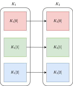
Figure 1: The OCNN loss applied to two kernels, $K_{1}$ and $K_{2}$, with 3 channels. The black arrows represent the full cross-correlation operation. OCNN is computed by performing the full cross-correlation of kernel channels with the same index.

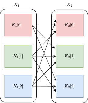
Figure 2: The Convolutional Similarity loss applied to two kernels, $K_{1}$ and $K_{2}$, with 3 channels. The black arrows represent the full cross-correlation operation. Convolutional Similarity is computed by performing the full cross-correlation of each kernel channel with all other channels of the other kernel.

4.3 Numerical Validation

In this section, experimental validation of the theory done in Section 4.2 is presented. The objective is to minimize the Convolutional Similarity to validate the effect it has on feature map orthogonality by performing the same experiments done in Section 4.1.

The same notations and variables from Section 4.1 are adopted. Let $K_{1},K_{2}\in\mathbb{R}^{N}$ and $X\in\mathbb{R}^{M}$ with values sampled from the same uniform distributions $\mathcal{U}(-1,1)$ and $\mathcal{U}(0,1)$, respectively. For every repetition of the experiment, optimization is carried it out until convergence, i.e., the near-total minimization of

$$\min_{K_{1},K_{2}}\|(K_{1}\circledast K_{2})\|_{2}^{2}.$$ (24)

In Table 3, the results of minimizing Convolutional Similarity on feature map similarity are presented. Compared to the results from Table 1, it is clear that Convolutional Similarity correlates considerably better with feature map similarity. As for the effect of totally minimizing Convolutional Similarity on feature map similarity, the results in Table 4 show that in all cases, feature map similarity is guaranteed to decrease. Additionally, feature maps are nearly orthogonal in all settings, as indicated by the recurring near-$100\%$ percentage decrease in feature map similarity. Another main difference between minimizing Convolutional Similarity and minimizing kernel similarity is that there are no risks of increased feature map similarity, as it always decreases.

N	Optimiser	(A) Correlation
		mean	std
3	Adam	0.80	0.27
	SGD	0.90	0.21
9	Adam	0.78	0.27
	SGD	0.85	0.25
16	Adam	0.71	0.30
	SGD	0.86	0.25

Table 3: The effect of minimizing Convolutional Similarity on feature map similarity. The correlation values are significantly higher compared to the results from Table 1. See Table 10 for the optimization hyper-parameters for each $N$.

N	Optimiser	(B) Reduction Frequency (%)	(C) Decrease (%)		(D) Increase (%)
			mean	std	mean	std
3	Adam	100	100	0.0	0	0
	SGD	100	99.91	1.28	0	0
9	Adam	100	99.98	0.23	0	0
	SGD	100	99.68	3.21	0	0
16	Adam	100	99.95	1.26	0	0
	SGD	100	99.78	3.04	0	0

Table 4: The effect of totally minimising Convolutional Similarity, on feature map similarity. In all cases, feature map similarity is guaranteed to decrease and approach orthogonality. See Table 10 for optimization hyper-parameters for each $N$.

The results in this section validate the theory presented in Section 4.2, as feature map similarity systematically decreases when Convolutional Similarity is fully minimized. Feature maps are nearly orthogonal, reaching around $99\%$ of percentage decrease in feature map similarity instead of $100\%$, due the numerical nature of the experiment, where convergence is considered to be the point where the loss is zero to two decimal places. So far, the results have only been demonstrated for full convolutions and full cross-correlations. Naturally, the question of whether they can be extended to the case of arbitrary padding values or not arises. This is answered in the next section.

5 Extension to Valid and Same Convolution/Cross-correlation

So far, we have established a sufficient condition on kernels for feature map orthogonality. However, it is based on the assumption of the full convolution/cross-correlation. In this section, an approximative approach is adopted to extend the use of Convolutional Similarity minimization to same and valid cross-correlation/convolution. The reason why this extension is important is that a lot of the most popular models do not use the full convolution/cross-correlation, but rather the same or the valid cross-correlation (e.g., Residual Neural Networks He et al. (2015)).

In what follows, we consider the general definition of the cross-correlation where the padding $P\in[0,N-1]$ explicitly appears

$$\forall i\in[N-1-P,M-1+P],(X\circledast K)[i]=\sum^{N-1}_{n=0}K[n]\cdot X[i+n-N+1].$$ (25)

Notice that

1. When $P=0$, Equation 25 corresponds to the definition of the valid cross-correlation.

2. When $P=N-1$, Equation 25 corresponds to the definition of the full cross-correlation.

3. When $P=\frac{N-1}{2}$, Equation 25 corresponds to the definition of the same cross-correlation.

Therefore, proving that the theory presented in Section 4.2 holds in the general case where the value of $P$ is arbitrary in the range $[0,N-1]$ would make Convolutional Similarity minimization applicable to a wider range of models. Adopting the same notations from Section 4.1, consider $F_{1}$ and $F_{2}$ such as, for $i\in[N-1-P,M-1+P]$ and $P\in[0,N-1]$

$$F_{1}[i]=(X\circledast K_{1})[i]=\sum^{N-1}_{n_{1}=0}K_{1}[n_{1}]\cdot X[n_{1}+1-N+1]$$ (26)

$$F_{2}[i]=(X\circledast K_{2})[i]=\sum^{N-1}_{n_{2}=0}K_{2}[n_{2}]\cdot X[n_{2}+-N+1].$$ (27)

We have

$$\langle F_{1},F_{2}\rangle=\sum^{M-1+P}_{i=N-1-P}F_{1}[i]\cdot F_{2}[i].$$ (28)

Notice that the formulation of $\langle F_{1},F_{2}\rangle$ here is different from the one in Equation 7. Using the same substitution to get Equation 9 in Section 4.2, we have

$$\langle F_{1},F_{2}\rangle=\sum^{N-1}_{n_{1}=0}\sum^{N-1}_{n_{2}=0}K_{1}[n_{1}]\cdot K_{2}[n_{2}]\sum^{M-N+P+n_{1}}_{i=n_{1}-P}X[i+n_{2}-n_{1}]\cdot X[i]$$ (29)

$$=-A-B+\sum^{N-1}_{n_{1}=0}\sum^{N-1}_{n_{2}=0}K_{1}[n_{1}]\cdot K_{2}[n_{2}]\sum^{M-1+n_{1}}_{i=1-N+n_{1}}X[i+n_{2}-n_{2}]\cdot X[i]$$ (30)

with

$$A=\sum^{N-1}_{n_{1}=0}\sum^{N-1}_{n_{2}=0}K_{1}[n_{1}]\cdot K_{2}[n_{2}]\sum^{n_{1}-P-1}_{i=n_{1}+1-N}X[i+n_{2}-n_{2}]\cdot X[i]$$ (31)

$$B=\sum^{N-1}_{n_{1}=0}\sum^{N-1}_{n_{2}=0}K_{1}[n_{1}]\cdot K_{2}[n_{2}]\sum^{M-1+n_{1}}_{i=M-N+P+n_{1}+1}X[i+n_{2}-n_{2}]\cdot X[i].$$ (32)

Based on Equation 14, we have

$$\langle F_{1},F_{2}\rangle=\langle(K_{1}\circledast K_{2}),(X\circledast X)_{[1-N,N-1]}\rangle-A-B.$$ (33)

$A$ and $B$ have $N\cdot N\cdot(N-P-1)$ terms, while $\langle(K_{1}\circledast K_{2}),(X\circledast X)_{[1-N,N-1]}\rangle$ has $N\cdot N\cdot(M+N-1)$ terms. Knowing that $N<<M$ (kernel dimension size is often significantly smaller than the input dimension size) and $P\leq N-1$, it is clear that $\langle(K_{1}\circledast K_{2}),(X\circledast X)_{[1-N,N-1]}\rangle$ has significantly more terms than $A$ and $B$, therefore, there is a high probability that

$$A+B<<\langle(K_{1}\circledast K_{2}),(X\circledast X)_{[1-N,N-1]}\rangle.$$ (34)

Therefore,

$$\langle F_{1},F_{2}\rangle\approx\langle(K_{1}\circledast K_{2}),(X\circledast X)_{[1-N,N-1]}\rangle.$$ (35)

The closer $P$ is to $N-1$, the closer the two sides of Equation 35 get. When $P=N-1$, we have

$$\langle F_{1},F_{2}\rangle=\langle(K_{1}\circledast K_{2}),(X\circledast X)_{[1-N,N-1]}\rangle.$$ (36)

Since, for $P\neq N-1$, $\langle(K_{1}\circledast K_{2}),(X\circledast X)_{[1-N,N-1]}\rangle$ is a good approximation of $\langle F_{1},F_{2}\rangle$, minimizing the former would most likely minimize the latter. This is verified numerically by performing the same numerical tests performed in Section 4.3. Outside the case of the full cross-correlation, the case where the risks of both sides of Equation 35 being different are high is when $P=0$, wherein the cross-correlation is called valid. Therefore, in the following experiments, we consider the valid cross-correlation and compute the quantities A, B, C, and D and present the results in Tables 5 and 6. The results are very similar to Tables 1 and 4, which shows that minimising Convolutional Similarity generally works for arbitrary values of $P$. Table 5 shows that the correlation between feature map similarity and Convolutional Similarity is significantly higher than the correlation between feature map similarity and kernel similarity, presented in Table 1. As for the effect of a near-total decrease in the Convolutional Similarity loss, Table 6 shows that in most cases, the decrease frequency is high. The smallest value B reached is $98.6\%$. As for the magnitude of the decrease in feature map similarity, it is near-total as well.

However, in some rare cases, minimizing Convolutional Similarity in the case of the valid cross-correlation can have an unpredictable effect on feature map similarity, as shown by some increases in feature map similarity in column $D$ in Table 6. This behavior is similar to minimizing kernel similarity (see Table 2). Nonetheless, this phenomenon is significantly less pronounced in the case of minimizing Convolutional Similarity for the valid cross-correlation, as the magnitudes are significantly less and the probability of it happening is very low (a probability of $0.014$ in the worst case in the experiments presented in Table 6).

All of these numerical results indicate that minimizing the Convolutional Similarity can be used in cases where the cross-correlation is not full (i.e., $P\neq N-1$). This conclusion is important as it allows its use in models that use arbitrary padding values. This result is further confirmed in Section 6.4, where Convolutional Similarity is minimized for a deep CNN that does not use the full cross-correlation.

N	Optimiser	(A) Correlation
		mean	std
3	Adam	0.798	0.272
	SGD	0.90	0.19
9	Adam	0.751	0.296
	SGD	0.86	0.23
16	Adam	0.77	0.28
	SGD	0.851	0.23

Table 5: The effect of minimizing Convolutional Similarity on feature map similarity when the cross-correlation is not full, i.e., $P<N-1$. The correlation values are significantly higher compared to the results from Table 1. See Table 11 for the optimization hyper-parameters for each $N$.

N	Optimiser	(B) Reduction Frequency (%)	(C) Decrease (%)		(D) Increase (%)
			mean	std	mean	std
3	Adam	100	99.99	0.02	0	0
	SGD	99.6	99.86	1.34	216.04	154.33
9	Adam	100	99.96	0.385	0	0
	SGD	99.5	99.57	3.77	3336.06	5322.40
16	Adam	99.9	99.80	2.49	688.54	0
	SGD	98.6	98.68	8.20	$10.90\times 10^{4}$	$40.35\times 10^{4}$

Table 6: The effect of totally minimising Convolutional Similarity, on feature map similarity. In all cases, feature map similarity is guaranteed to decrease and approach orthogonality. See the appendix (Table 11) for optimization hyper-parameters for each $N$.

6 Experiments and Results

6.1 Experimental Setting

Experiments are conducted on CIFAR-10 Krizhevsky and Hinton (2009), a classification dataset with 50,000 training images and 10,000 test images. No preprocessing or data augmentation are applied to the images.

Minimising Convolutional Similarity can be done in two ways: (1) it can be minimized before training, in this case, it would be an iterative initialization scheme, where it could be perceived as a form of pretraining as well, according to Algorithm 1, (2) it can be minimized during training, in this case, it would be a regularisation method, according to Algorithm 2.

Algorithm 1 Convolutional Similarity minimization as an iterative initialization scheme. $\theta$ are the parameters of the model and $K^{(j)}$ are the kernels of the $j$-th convolutional layer. $L_{task}$ and $L_{CS}$ are the training task loss function and the Convolutional Similarity loss function, respectively. Before the model is trained, $L_{CS}$ is minimized for a number of iterations $I$.

for $I$ iterations do

     One optimization step of the Convolutional Similarity minimization

$$\nabla_{\theta}\sum^{M-1}_{j=0}L_{CS}(K^{(j)})$$

end for

for training epochs do

     One training epoch of the model.

$$\nabla_{\theta}L_{task}$$

end for

Algorithm 2 Convolutional Similarity minimization as a regularization term. $\theta$ are the parameters of the model and $K^{(j)}$ are the kernels of the $j$-th convolutional layer. $L_{task}$ and $L_{CS}$ are the training task loss function and the Convolutional Similarity loss function, respectively. $L_{CS}$ is minimized during the training of the model and is used as a regularisation term with a weighting factor $\beta$.

for training epochs do

     Convolutional Similarity is minimized with every epoch

$$\nabla_{\theta}\left(L_{task}+\beta\cdot\sum^{M-1}_{j=0}L_{CS}(K^{(j)})\right)$$

end for

The experiments are divided into two parts:

1. Preliminary experiments on shallow CNNs where the two aforementioned methods of minimizing Convolutional Similarity are explored and used to select whichever one yields the best results with the least amount of computational cost.

2. Experiments on a deep model, ResNet18 He et al. (2015) to observe the benefits of our proposed method. This experimental part is also used to validate Section 5, where it is stated that Convolutional Similarity minimization can be extended to convolutional layers with arbitrary padding values and not only $P=N-1$ (the full cross-correlation).

6.2 Iterative Initialisation vs Regularisation

CNN1
Conv2d(3, 64, 3, 2)
BatchNorm2d(64)
LeakyReLU(0.2)
MaxPool2d(2, 2)
Conv2d(64, 64, 3, 2)
BatchNorm2d(64)
LeakyReLU(0.2)
MaxPool2d(2, 2)
Conv2d(64, 64, 3, 2)
BatchNorm2d(64)
LeakyReLU(0.2)
MaxPool2d(2, 2)
Conv2d(64, 64, 3, 2)
BatchNorm2d(64)
LeakyReLU(0.2)
MaxPool2d(2, 2)
Linear(576, 10)

CNN2
Conv2d(3, 128, 3, 2)
BatchNorm2d(128)
LeakyReLU(0.2)
MaxPool2d(2, 2)
Conv2d(128, 128, 3, 2)
BatchNorm2d(128)
LeakyReLU(0.2)
MaxPool2d(2, 2)
Conv2d(128, 128, 3, 2)
BatchNorm2d(128)
LeakyReLU(0.2)
MaxPool2d(2, 2)
Conv2d(128, 128, 3, 2)
BatchNorm2d(128)
LeakyReLU(0.2)
MaxPool2d(2, 2)
Linear(1152, 10)

Table 7: The configurations of CNN1 and CNN2 with Conv2d(input channels, output channels, kernel size, padding), BatchNorm2d(output channels), MaxPool2d(kernel size, stride) and Linear(input units, output units).

In this set of experiments, the two methods of minimizing Convolutional Similarity are tested. The objective is to experimentally test which of the two leads to better results with the least amount of computational overhead. As the number of feature maps increases, computing the gradients of the Convolutional Similarity loss can significantly increase as well. Therefore, we pick two CNNs with the same architecture but different numbers of feature maps and apply Convolutional Similarity minimization to them. The configurations are presented in Table 7. They consist of convolutional blocks with Batch Normalisation Ioffe and Szegedy (2015), LeakyReLU activation functions, and maxpooling. When Convolutional Similarity minimization is used as a regularization method, SGD is with a learning rate of 0.01 is used for optimization. When it is used as an iterative initialization method, Adam is used with a learning rate of 0.001 to minimize the Convolutional Similarity loss prior to training. Afterward, SGD with a learning rate of 0.01 is used to minimize the Cross Entropy loss function. In both cases, the batch size is 512. The models are trained for 100 epochs and the top test accuracies are retained.

Model	Test Accuracy (%)
CNN1 (baseline)	74.66
CNN1 ($I=500$)	79.16
CNN1 ($\beta=0.001$)	77.16
CNN2 (baseline)	76.87
CNN2 ($I=500$)	82.33
CNN2 ($\beta=0.001$)	80.00

Table 8: Top test accuracy for CNN1 and CNN2. The model that uses Convolutional Similarity as an iterative initialization method leads to the highest test accuracy.

Table 8 shows the top-1 test accuracies for the baseline models, the ones trained with $I=500$ (where $I$ is the number of Convolutional Similarity minimization iterations prior to training, refer to Algorithm 1) and the ones trained with $\beta=0.001$ (where $\beta$ is the weighting parameter for the regularization term, refer to Algorithm 2). Minimizing the Convolutional Similarity of both models leads to an increase in test accuracy, whether it is used as a regularization method or as an iterative initialization method. The latter, however, leads to the best performance.

Another advantage of the iterative initialization approach is that it introduces less computational overhead compared to the regularization method. The latter adds 9800 (98 per epoch) optimization steps of the Convolutional Similarity loss, while the iterative initialization method adds only 500 steps (as $I=500$). Even more, it could be perceived as a form of pre-training: one can minimize the Convolutional Similarity loss of a model once, which can then be saved and used on different datasets and different tasks, without having to minimize the Convolutional Similarity loss once again. However, in this case, one must be careful about the learning rate to be used during training. A large learning rate often leads to a phenomenon akin to catastrophic forgetting Kirkpatrick et al. (2017), where the model forgets the weights learned in the iterative initialization phase. Since the Convolutional Similarity function is convex, it is straightforward to find the proper range of learning rates. With a learning rate that is not too large, the Convolutional Similarity loss remains very low during training even when $\beta=0$, as can be shown in Figure 3 shows the Convolutional Similarity loss curves for the CNN2 baseline, CNN2 trained with $I=500$ and CNN2 trained with $\beta=0.001$.

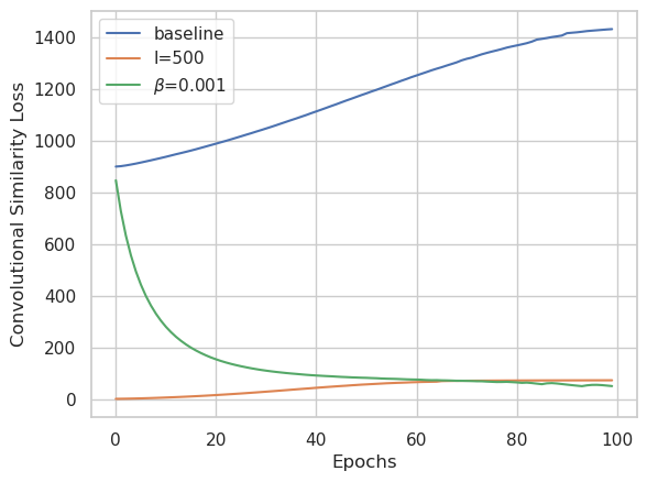
Figure 3: Convolutional Similarity loss curves for (a) the baseline, (b) $I=500$, and (c) $\beta=0.001$. Even when Convolutional Similarity is minimized prior to training, its value remains low.

Additionally, the results show that using Convolutional Similarity as an iterative initialization method accelerates convergence. Figures 4 and 5 show the evolution of the loss and the training accuracy during training for both models. In Figure 4, one can clearly observe that the classification loss decreases faster when $I=500$, compared to the baseline. However, the loss of the models trained with $\beta=0.001$ decreases slower, which makes sense considering that, in this case, the Convolutional Similarity loss was used as a regularisation term, and therefore can interfere with the decrease of the classification loss. This phenomenon is more apparent when the classification loss reaches low values: the gradients of the Convolutional Similarity are more prone to cause oscillations in the classification loss. Despite the oscillations, using the Convolutional Similarity regularisation leads to higher test accuracy. These observations are further validated when inspecting the train accuracy in Figure 5: for $I=500$, CNN1 and CNN2 reach $100\%$ train accuracy around 40 epochs and 20 epochs, respectively, before the baselines do. The oscillations observed in the loss of CNN1 in Figure 4 are reflected on the train accuracy in Figure 5. Nonetheless, even when $\beta=0.001$, both models reach $100\%$ train accuracy before the baselines do.

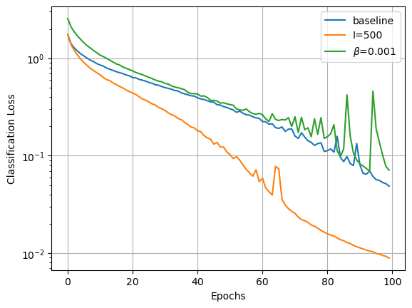
(a) Classification loss of CNN1

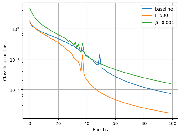
(b) Classification loss of CNN2

Figure 4: The evolution of the classification losses for CNN1 and CNN2. When $I=500$, the loss decreases faster than the baseline. When $\beta=0.001$, the loss can go through oscillations when it reaches low values. The graph uses a logarithmic scale on the y-axis.

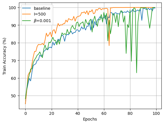
(a) Train accuracy of CNN1

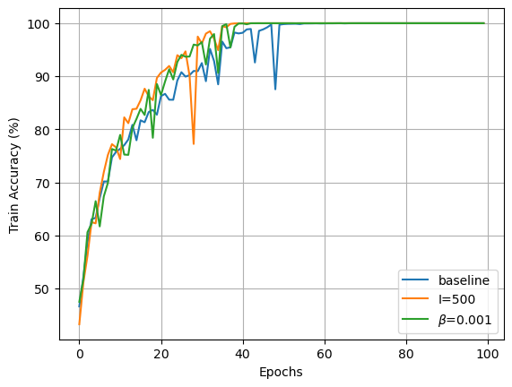
(b) Train accuracy of CNN2

Figure 5: Train accuracy of CNN1 and CNN2. Using Convolutional Similarity accelerates training: models reach $100\%$ train accuracy before the baseline models.

6.3 More Efficient Capacity Use

In this section, we explore how much capacity (i.e., trainable parameters) should be added to the CNN2 baseline to be able to match the performance of CNN1 with $I=500$. As a reminder, CNN1 and CNN2 have the same architecture. The only difference is that CNN2 has twice as many feature maps per layer: CNN1 has 118,858 parameters while CNN2 has 458,890, that is 3.86 times as many trainable parameters. Yet, CNN1 trained with Convolutional Similarity outperforms the CNN2 baseline ($79.16\%$ vs $76.87\%$). For CNN2 to slightly outperform CNN1 with $I=500$, it took eight-fold feature maps per layer (512 feature maps per layer). In this case, CNN2 has 7,143,946 trainable parameters, that is 60.10 times as many parameters as CNN1. With 60.10 more parameters, CNN2 achieved an accuracy of $79.78\%$, vs $79.16\%$ achieved by CNN1 trained with $I=500$. This indicates that the proposed method can lead to higher performance with considerably fewer parameters.

6.4 Experiments on a Deep CNN

To further confirm the benefits of minimizing Convolutional Similarity on CNNs, we consider ResNet18. We apply the iterative initialization method described in Algorithm 1 with $I=200$ and then train the model on CIFAR10 for 50 epochs with SGD with different combinations of learning rates and batch sizes. The objective of these experiments is to see to which extent a deep CNN can benefit from minimizing the Convolutional Similarity loss prior to training. Convolutional Similarity is minimized using Adam with a learning rate of 0.001 and $(\beta_{1},\beta_{2})=(0.5,0.999)$.

The results for different configurations is presented in Figure 6. In all cases, using our method on ResNet18 results in higher accuracy. In some cases, the model benefited significantly from minimizing Convolutional Similarity. For example, in the case where the learning rate is $0.001$ and the batch size is $128$, the increase in accuracy is $20\%$. Note that in all cases, no data augmentation nor normalization were applied to the dataset. These results confirm the benefit of using our method in different settings.

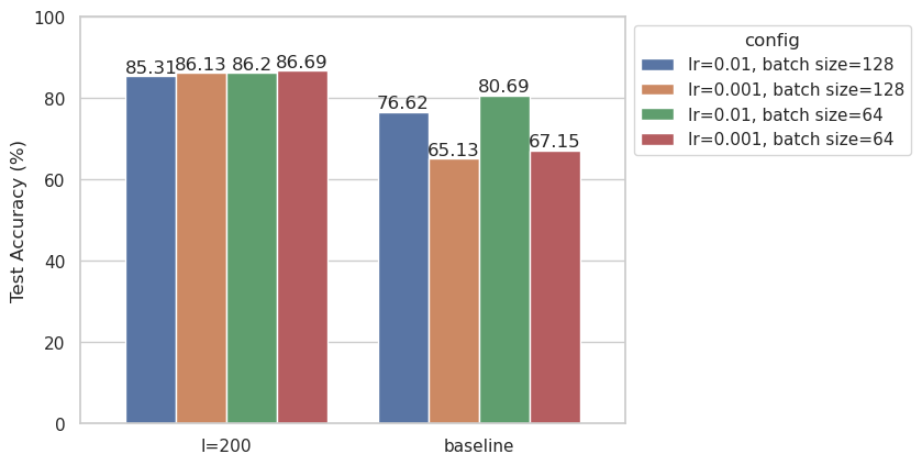
Figure 6: Test accuracy of different configurations of ResNet18 trained with and without Convolutional Similarity minimization, used as an iterative initialization method ($I=200$). In all cases, using our method leads to a significant increase in performance.

However, one might wonder about the optimal value for $I$ for the model to benefit from Convolutional Similarity minimization. To explore this, we train ResNet18 for different values of $I\in\{0,10,20,40,60,80,100,120,140,160,180,200\}$ to see how accuracy improves depending on $I$. We set the learning rate to 0.01 and the batch size to 64 and train the model for 50 epochs. The results are presented in Figure 7, where we can see that the model can reap the biggest part of the gain in accuracy with $I<60$, which suggests that $I$ can be as small as $10$ and yet can lead to better performance. This conclusion is important for deeper models where computing Convolutional Similarity gradients might prove computationally expensive.

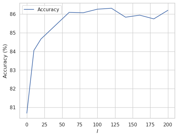
Figure 7: Test accuracy of ResNet18 using different values for the number of iterations $I$ in the iterative initialization scheme. Most of the gains in accuracy occur for $I<60$.

7 Limitations: Momentum and Large Learning Rates

While the results indicate that minimizing Convolutional Similarity is beneficial to CNNs, there exists some limitations to our method, which are twofold:

1. The iterative initialization method does not function well in two cases: (1) when the original task loss (e.g., classification) is minimized using optimizers with momentum (e.g., Adam and SGD with momentum) and (2) with large learning rates. It has been observed that optimizers with momentum lead to a significant increase in weight magnitude, which increases the Convolutional Similarity loss. The same observation was made in Heo et al. (2021). As for large learning rates, they push the weights outside of the region where Convolutional Similarity is minimal. Optimizers with momentum work better with Convolutional Similarity minimization as a regularisation method, but the latter leads to a larger computational overhead and adds oscillations near the end of training where the gradients of the original task loss are weaker due to smaller loss values. This, however, can be potentially solved by decreasing $\beta$ proportionally to the magnitude of the original task loss.

2. While the Convolutional Similarity loss function is independent of the size of the input, which gives it a great computational advantage over explicitly minimizing feature map similarity, it can add a significant computational overhead depending on the number of input and output channels. Therefore, with limited computational resources, training a model with Convolutional Similarity minimization can take a significant amount of time. For reference, on an Nvidia A5000 GPU, one optimization step of Convolutional Similarity minimization on ResNet18 can take around 90 seconds. Optimizing the CUDA implementation of Convolutional Similarity forward and backward passes could lead to less computational overhead.

8 Conclusion and Future Work

In this work, we prove, theoretically and empirically, that kernel orthogonality does not necessarily lead to a decrease in feature map similarity, in contrast to common belief. Based on the theoretical analysis, a new loss term is proposed: Convolutional Similarity, which can be minimized in two ways, either as a regularization term or as an iterative initialization scheme. Minimizing Convolutional Similarity decreases feature map similarity and leads to better CNN performance, as the capacity is used more efficiently. As future work, it would be interesting to explore how to couple our method with optimizers with momentum, as discussed in Section 7. Additionally, the effect of our method on generative frameworks like Generative Adversarial Networks Goodfellow et al. (2014) could be another interesting path to explore.

9 Appendix

9.1 Numerical Validation Experiments Configurations

N	Optimizer	Learning Rate	Number of Iterations
3	Adam	0.1	250
	SGD	0.1	250
9	Adam	0.1	250
	SGD	0.1	250
16	Adam	0.1	250
	SGD	0.1	300

Table 9: Optimization hyperparameters for kernel cosine similarity minimization experiments.

N	Optimizer	Learning Rate	Number of Iterations
3	Adam	0.1	300
	SGD	0.2	350
9	Adam	0.1	400
	SGD	0.07	550
16	Adam	0.2	450
	SGD	0.035	1500

Table 10: Optimization hyperparameters for Convolutional Similarity optimization experiments.

N	Optimizer	Learning Rate	Number of Iterations
3	Adam	0.1	300
	SGD	0.1	300
9	Adam	0.1	300
	SGD	0.05	400
16	Adam	0.05	500
	SGD	0.01	700

Table 11: Optimization hyperparameters for kernel cosine similarity minimization experiments.

References

- pyt [2023] Convolutional layer documentaion - PyTorch, 2023. URL https://pytorch.org/docs/stable/generated/torch.nn.Conv2d.html. Online; accessed 22 July 2023.
- ten [2023] Convolutional layer implementation - TensorFlow and Keras, 2023. URL https://github.com/keras-team/keras/blob/v3.3.3/keras/src/layers/convolutional/conv2d.py#L5-L126. Online; accessed 22 July 2023.
- Achour et al. [2022] E. M. Achour, F. Malgouyres, and F. Mamalet. Existence, stability and scalability of orthogonal convolutional neural networks. Journal of Machine Learning Research, 23(347):1–56, 2022. URL http://jmlr.org/papers/v23/22-0026.html.
- Bansal et al. [2018] N. Bansal, X. Chen, and Z. Wang. Can we gain more from orthogonality regularizations in training deep CNNs? 32nd Conference on Neural Information Processing Systems (NeurIPS 2018), 2018.
- Cogswell et al. [2016] M. Cogswell, F. Ahmed, R. Girshick, L. Zitnick, and D. Batra. Reducing overfitting in deep networks by decorrelating representations. International Conference on Learning Representations, 2016.
- Denil et al. [2013] M. Denil, B. Shakibi, L. Dinh, M. A. Ranzato, and N. de Freitas. Predicting parameters in deep learning. In Advances in Neural Information Processing Systems, volume 26, 2013.
- Goodfellow et al. [2014] I. J. Goodfellow, J. Pouget-Abadie, M. Mirza, B. Xu, D. Warde-Farley, S. Ozair, A. Courville, and Y. Bengio. Generative adversarial networks, 2014. URL https://arxiv.org/abs/1406.2661.
- He et al. [2015] K. He, X. Zhang, S. Ren, and J. Sun. Deep residual learning for image recognition. 2016 IEEE Conference on Computer Vision and Pattern Recognition, 2015.
- Heo et al. [2021] B. Heo, S. Chun, S. J. Oh, D. Han, S. Yun, G. Kim, Y. Uh, and J.-W. Ha. Adamp: Slowing down the slowdown for momentum optimizers on scale-invariant weights, 2021. URL https://arxiv.org/abs/2006.08217.
- Ioffe and Szegedy [2015] S. Ioffe and C. Szegedy. Batch normalization: Accelerating deep network training by reducing internal covariate shift, 2015.
- Jaderberg et al. [2014] M. Jaderberg, A. Vedaldi, and A. Zisserman. Speeding up convolutional neural networks with low rank expansions, 2014.
- Karras et al. [2021] T. Karras, M. Aittala, S. Laine, E. Härkönen, J. Hellsten, J. Lehtinen, and T. Aila. Alias-free generative adversarial networks, 2021. URL https://arxiv.org/abs/2106.12423.
- Kingma and Ba [2015] D. Kingma and J. Ba. Adam: A method for stochastic optimization. International Conference on Learning Representations (ICLR 2015), 2015.
- Kirkpatrick et al. [2017] J. Kirkpatrick, R. Pascanu, N. Rabinowitz, J. Veness, G. Desjardins, A. A. Rusu, K. Milan, J. Quan, T. Ramalho, A. Grabska-Barwinska, D. Hassabis, C. Clopath, D. Kumaran, and R. Hadsell. Overcoming catastrophic forgetting in neural networks. Proceedings of the National Academy of Sciences, 114(13):3521–3526, Mar. 2017. ISSN 1091-6490. doi: 10.1073/pnas.1611835114. URL http://dx.doi.org/10.1073/pnas.1611835114.
- Krizhevsky and Hinton [2009] A. Krizhevsky and G. Hinton. Learning multiple layers of features from tiny images. Technical report, University of Toronto, Toronto, Ontario, 2009.
- Krizhevsky et al. [2012] A. Krizhevsky, I. Sutskever, and G. E. Hinton. Imagenet classification with deep convolutional neural networks. In Advances in Neural Information Processing Systems. Curran Associates, Inc., 2012.
- Le Cun et al. [1989] Y. Le Cun, J. S. Denker, and S. A. Solla. Optimal brain damage. In Proceedings of the 2nd International Conference on Neural Information Processing Systems, NIPS’89, page 598–605, Cambridge, MA, USA, 1989. MIT Press.
- LeCun et al. [1989] Y. LeCun, B. Boser, J. S. Denker, D. Henderson, R. E. Howard, W. Hubbard, and L. D. Jackel. Backpropagation applied to handwritten zip code recognition. Neural Computation, 1(4):541–551, 1989.
- Rodríguez et al. [2017] P. Rodríguez, J. Gonzàlez, G. Cucurull, J. M. Gonfaus, and X. Roca. Regularizing CNNs with locally constrained decorrelations. In International Conference on Learning Representations, 2017.
- Ronneberger et al. [2015] O. Ronneberger, P. Fischer, and T. Brox. U-Net: Convolutional networks for biomedical image segmentation. Medical Image Computing and Computer-Assisted Intervention, 9351:234–241, 10 2015.
- Sauer et al. [2023] A. Sauer, T. Karras, S. Laine, A. Geiger, and T. Aila. Stylegan-t: Unlocking the power of gans for fast large-scale text-to-image synthesis, 2023. URL https://arxiv.org/abs/2301.09515.
- Shannon [1948] C. E. Shannon. A mathematical theory of communication. The Bell System Technical Journal, 27:379–423, 1948.
- Simonyan and Zisserman [2015] K. Simonyan and A. Zisserman. Very deep convolutional networks for large-scale image recognition. 3rd International Conference on Learning Representations, ICLR 2015, 2015.
- Wang et al. [2020] J. Wang, Y. Chen, R. Chakraborty, and S. X. Yu. Orthogonal convolutional neural networks. In IEEE Conference on Computer Vision and Pattern Recognition (CVPR 2020), 2020.