textcite Textcite 3GPPshort=3GPP, long=3rd Generation Partnership Project, 4Gshort=4G, long=4${}^{\text{th}}$ Generation, 5Gshort=5G, long=5${}^{\text{th}}$ Generation, 5GV2Xshort=5G-V2X, long=5${}^{\text{th}}$ Generation Cellular V2X, ACIshort=ACI, long=Adjacent Channel Interference, AGCshort=AGC, long=Automatic Gain Control, AIshort=AI, long=Artificial Intelligence, AoIshort=AoI, long=Age of Information, APshort=AP, long=Access Point, APIshort=API, long=Application Programming Interface, AWGNshort=AWGN, long=Additive White Gaussian Noise, BERshort=BER, long=Bit Error Probability, BPSKshort=BPSK, long=Binary Phase Shift Keying, CSIshort=CSI, long=Channel State Information, CSMAshort=CSMA, long=Carrier-Sense Multiple Access, CV2Xshort=C-V2X, long=Cellular V2X, D2Dshort=D2D, long=Device-to-Device, DESshort=DES, long=Discrete Event Simulation, eNBshort=eNB, long=eNodeB, FCCshort=FCC, long=Federal Communications Commission, FDMAshort=FDMA, long=Frequency-Division Multiple Access, FSMshort=FSM, long=Finite State Machine, gNBshort=gNB, long=gNodeB, GUIshort=GUI, long=Graphical User Interface, HARQshort=HARQ, long=Hybrid Automatic Repeat reQuest, ICshort=IC, long=In Coverage, JCASshort=JCAS, long=Joint Communication and Sensing, WLANshort=WLAN, long=Wireless Local Area Network, LOSshort=LoS, long=Line of Sight, LTEshort=LTE, long=Long Term Evolution, LTEV2Xshort=LTE-V2X, long=Cellular V2X, MACshort=MAC, long=Medium Access Control, MECshort=MEC, long=Mobile Edge Computing, MIshort=MI, long=Mutual Information, MIMOshort=MIMO, long=Multiple Input Multiple Output, MLshort=ML, long=Machine Learning, MLOshort=MLO, long=Multi-Link Operation, MUMIMOshort=MU-MIMO, long=Multi-User MIMO, MPCshort=MPC, long=Model Predictive Control, short-indefinite=an NRshort=NR, long=New Radio, OFDMshort=OFDM, long=Orthogonal Frequency-Division Multiplexing, OFDMAshort=OFDMA, long=Orthogonal Frequency-Division Multiple Access, OoCshort=OoC, long=Out of Coverage, PC5short=PC5, long=PC5, PDRshort=PDR, long=Packet Delivery Ratio, PDFshort=PDF, long=Probability Density Function, PHYshort=PHY, long=Physical Layer, PMFshort=PMF, long=Probability Mass Function, PSKshort=PSK, long=Phase Shift Keying, QAMshort=QAM, long=Quadrature Amplitude Modulation, QOSshort=QoS, long=Quality of Service, QBPSKshort=QBPSK, long=Quadrature Binary Phase Shift Keying, QPSKshort=QPSK, long=Quadrature Phase Shift Keying, RUshort=RU, long=Resource Unit, SINRshort=SINR, long=Signal to Interference plus Noise Ratio, short-indefinite=an SIRshort=SIR, long=Signal to Interference Ratio, SNRshort=SNR, long=Signal to Noise Ratio, STAshort=STA, long=Station, TDMAshort=TDMA, long=Time-Division Multiple Access, UEshort=UE, long=User Equipment, URLLCshort=URLLC, long=Ultra-Reliable Low-Latency Communication, Uushort=Uu, long=User to Network Interface, V2Vshort=V2V, long=Vehicle to Vehicle communication, V2Xshort=V2X, long=Vehicle to Everything, VLCshort=VLC, long=Visible Light Communication, VRUshort=VRU, long=Vulnerable Road Users, WHDshort=WHD, long=Weighted Hamming Distance, ZOHshort=ZOH, long=Zero Order Hold,

DIPARTIMENTO DI INGEGNERIA DELL’INFORMAZIONE

Corso di Laurea Magistrale

in Ingegneria Informatica

Tesi di Laurea

Statistical Analysis to Support
CSI-Based Sensing Methods
Analisi Statistica a Supporto
di Metodi di Misura Basati su CSI

Relatore: Chiar.mo Prof. Renato Lo Cigno

Laureanda:

Elena Tonini

Matricola n. 727382

Anno Accademico 2023/24

Sommario

Prendendo spunto dal lavoro della Tesi di Laurea Triennale intitolata “Analysis and Characterization of Wi-Fi Channel State Information”, questa tesi amplia e approfondisce la ricerca conducendo un’analisi dettagliata delle CSI, offrendo nuovi approcci che si spingono oltre i risultati dello studio originale. L’obiettivo del lavoro è estendere la rappresentazione matematica e statistica di un canale wireless attraverso lo studio del comportamento e dell’evoluzione nel tempo e nella frequenza delle CSI.

Le CSI forniscono una descrizione ad alto livello del comportamento di un segnale che si propaga da un trasmettitore a un ricevitore, rappresentando così la struttura dell’ambiente che il segnale attraversa. Questa conoscenza può essere utilizzata per effettuare ambient sensing, una tecnica che permette di estrarre informazioni rilevanti sull’ambiente di propagazione in funzione delle proprietà che il segnale presenta al ricevitore, dopo aver interagito con le superfici degli oggetti presenti nello spazio analizzato. L’ambient sensing svolge già un ruolo essenziale nelle nuove reti wireless come 5G e Beyond 5G; il suo impiego nelle applicazioni di Joint Communication and Sensing e per l’ottimizzazione della propagazione del segnale tramite beamforming potrebbe supportare ambient sensing cooperativo efficiente anche nelle reti veicolari, consentendo la Cooperative Perception e aumentando di conseguenza la sicurezza stradale.

A causa della mancanza di ricerca sulla caratterizzazione delle CSI, l’attuale studio intraprende un’analisi della struttura delle CSI raccolte in un ambiente sperimentale controllato, al fine di descriverne le proprietà statistiche. I risultati potrebbero fornire un approccio matematico di supporto alle attività di environment classification e di movement recognition che attualmente sono eseguite solo tramite approcci basati su Machine Learning, introducendo invece efficienti algoritmi dedicati.

Summary

Building upon the foundational work of the Bachelor’s Degree Thesis titled “Analysis and Characterization of Wi-Fi Channel State Information”, this thesis significantly advances the research by conducting an in-depth analysis of CSIs, offering new insights that extend well beyond the original study. The goal of this work is to broaden the mathematical and statistical representation of a wireless channel through the study of CSI behavior and evolution over time and frequency.

CSI provides a high-level description of the behavior of a signal propagating from a transmitter to a receiver, thereby representing the structure of the environment where the signal propagates. This knowledge can be used to perform ambient sensing, a technique that extracts relevant information about the surroundings of the receiver from the properties of the received signal, which are affected by interactions with the surfaces of the objects within the analyzed environment. Ambient sensing already plays an essential role in new wireless networks such as 5G and Beyond 5G; its use in Joint Communication and Sensing applications and for the optimization of signal propagation through beamforming could also enable the implementation of efficient cooperative ambient sensing in vehicular networks, facilitating Cooperative Perception and, consequently, increasing road safety.

Due to the lack of research on CSI characterization, this study aims to begin analyzing the structure of CSI traces collected in a controlled experimental environment and to describe their statistical properties. The results of such characterization could provide mathematical support for environment classification and movement recognition tasks that are currently performed only through Machine Learning techniques, introducing instead efficient, dedicated algorithms.

Contents

1. 1 Introduction
2. 2 Wi-Fi Fundamentals
   1. 2.1 Modulation Techniques
   2. 2.2 OFDM
   3. 2.3 802.11ax Standard Version
   4. 2.4 802.11be Standard Version
   5. 2.5 CSI Structure
3. 3 Background and Previous Results
   1. 3.1 Data Collection
   2. 3.2 Amplitude Evolution in Time
   3. 3.3 Amplitude Relative Frequency Observation
   4. 3.4 Amplitude Increments and Auto-Correlation
   5. 3.5 Amplitude Increments Analysis
4. 4 Experimental Setup
   1. 4.1 Collected data
   2. 4.2 Additional available dataset
5. 5 Notation
6. 6 Normalization and Quantization
   1. 6.1 Estimate of the Increments Process
   2. 6.2 Quantization and Mapping
   3. 6.3 Visualization of the Normalization and Quantization Processes
7. 7 Mutual Shannon Information
   1. 7.1 Future Research Directions
8. 8 Weighted Hamming Distance
9. 9 CSI Processing
10. 10 Results of the Normalization and Quantization Processes
11. 11 Results of the Analysis of the Weighted Hamming Distance
    1. 11.1 Results on the Collected Dataset
    2. 11.2 Results on the AntiSense dataset
12. 12 Conclusions and Future Work
    1. Acknowledgments
13. A Detailed Classification of Collected Data
14. B Normalized Average WHD of the AntiSense Dataset

1     Introduction

With the ever-increasing applications of wireless telecommunication networks in all aspects of everyday life, ensuring users’ security and privacy has become an increasingly delicate field of study requiring dedicated research.

As users across the world are becoming accustomed to approaching Wi-Fi as a means of quickly transferring their own data, the ongoing development of this technology is both guaranteeing more users access to network coverage and high bit rates and raising awareness about previously unforeseen threats to users’ security [1]. Aside from the challenges of Wi-Fi managed through the introduction of cryptographic protocols employed to ensure users’ security when accessing the Internet [2], some features of Wi-Fi can still be exploited by attackers to violate users’ privacy. Specifically, it may become more straightforward in the near future to perform attacks based on Wi-Fi CSI [3, 4, 5].

CSI are pieces of information associated with packets transmitted on a Wi-Fi channel and whose structure allows for the description of the behavior of a signal propagating from a transmitter to a receiver. Essentially, they provide a numerical representation of how the signal bounces off the surfaces it meets during its propagation by including information about the signal’s phase shift and attenuation [6]. CSI do not intrinsically qualify as tools that can be exploited to perform attacks on wireless networks, but rather as features that should be used to improve the quality of telecommunications over Wi-Fi. Newly developed technologies benefit from the use of CSI when implementing MIMO techniques and improving channel equalization.

In fact, CSI can also be used to perform ambient sensing, a technique that extracts spatial information about the environment in which a signal propagates. Depending on the reflection, scattering, and absorption of the signal by the surroundings of both transmitter and receiver, the content of a CSI is altered and it can be interpreted as a representation of the environment itself. The content of a CSI becomes a useful descriptor of both the static and dynamic structure of an environment, while also allowing to locate electronic devices within it. Moreover, it is not necessary for a person to be carrying a communication device to be correctly located within the environment through the analysis of CSI content, as the propagating signal will interact with the person’s body regardless of the presence of any other electronic device [7, 8]. This allows to both identify the position of the person and give an idea about their movements around the environment based solely on the properties the signal displays once it is received and its associated CSI are extracted [9].

Of course, this property of CSI may be exploited by attackers to locate users within a given environment, violating their privacy without giving them the chance to defend themselves from sensing-based attacks [10]. Research conducted in this field has identified signal jamming and information obfuscation — which do not interfere with the quality and understandability of the transmitted content at the receiver — as possible countermeasures to prevent attackers from obtaining sensing information directly from extracted CSI [11, 12].

The feature that makes sensing attacks apparently easy to carry out is that to effectively perform ambient sensing, the only requirements are that a fixed transmitter be placed within the analyzed environment and that a sensing receiver — which should also be in a fixed position so as not to externally alter the CSI content — be used to capture and analyze the extracted CSI.

The feasibility of ambient sensing, for the time being, has only been tested in indoor environments using Wi-Fi-based technologies [4, 13], but multiple applications could benefit from its implementation in outdoor locations and from the use of different technologies (e.g., cellular networks). Specifically, a useful extension to ambient sensing as we know it would be JCAS, an approach that allows multiple parties to share information alongside the more “traditional” sensing activity.

JCAS is expected to play a significant role in 5G New Radio and Beyond 5G networks, where the concept of “sharing ambient sensing information” becomes more relevant. As communications rely on increasingly higher frequencies (over 20-30 GHz), difficulties may arise when LOS between transmitter and receiver becomes strictly required for communications to effectively take place, as omnidirectional antennae no longer provide sufficient power to support data exchange at such frequencies. Communications at high frequencies undergo significant signal attenuation during outdoor propagation, requiring the implementation of beamforming to increase the directionality of a transmitter radiation pattern: this approach ensures that the pattern covers only the area where the targeted receiver is expected to be, significantly reducing power waste compared to omnidirectional antennae and increasing efficiency in communication through an increment in power density in the direction of the receiver. Without beamforming, guaranteeing that all receiving devices have LOS with an omnidirectional transmitter would be infeasible [14].

As implementing beamforming remains technologically challenging, the introduction of ambient sensing may help identify obstacles along the signal propagation path and automatically steer beams or move transmission to a device that guarantees better QOS when operating in a mesh-like network topology.

Other fields of research may draw advantage from the implementation of CSI-based JCAS, specifically when high data rates are required. Above all others, autonomous vehicle networks may see the implementation of JCAS as a tool to improve the quality of shared sensing information and to make the process of sharing such data more efficient. The main requirement for autonomous vehicles to perform cooperative ambient sensing is the availability of high data rates, as each vehicle should ultimately be able to share tens of gigabytes of information per second with all surrounding vehicles [15]. Cooperative ambient sensing allows all vehicles participating in the activity to build a full virtual representation of the surrounding real world, deriving information on static obstacles, VRU, other vehicles, etc. from what has been sensed and shared by the others through V2V [16]. This approach, albeit currently infeasible on a large scale given the available technologies and supported data rates, would greatly improve the performance of autonomous driving applications, allowing vehicles to identify obstacles that are hidden from their own sensors through what has been detected and shared by surrounding road users [17].

Implementing a network whose users are allowed to share gigabytes of data per second (with each transmission possibly being similar to previous ones, as sensor data may not change drastically from one second to another, especially when travelling at low speed) while simultaneously granting a minimum QOS in a safety-critical application is not a simple task; nonetheless, it may benefit from the introduction of CSI-based ambient sensing to reduce the necessity for an autonomous vehicle to share raw sensor data with all surrounding vehicles, by instead only sending the extracted CSI as already-parsed information about the surrounding environment.

Studies are already being conducted on the possibility of exploiting shared frequencies and hardware when performing JCAS to improve spectrum efficiency and reduce hardware cost: this could result in larger applicability of JCAS, even in contexts where it is currently infeasible [18, 19], with cheaper implementations on a larger scale from which also applications in autonomous driving could greatly benefit.

State-of-the-art mechanisms to perform ambient sensing mainly consist of Artificial Intelligence and Machine Learning applications [20], but they often require more computational resources and resolution time than are available, especially when working with safety-critical or real-time applications. Moreover, understanding the mathematical characterization of the electromagnetic channel supporting the transmission may result in efficient dedicated algorithms to extract CSI and gain useful information to make JCAS more efficient.

This work serves as a continuation of the introductory study proposed in the Bachelor’s Degree Thesis titled “Analysis and Characterization of Wi-Fi Channel State Information” [21]. The goal of this work is to study the statistical properties of a Wi-Fi channel through the analysis of CSI behaviour and evolution in time and frequency. This analytical approach aims to help identify and describe some channel characteristics that can be used by AI and ML techniques to classify and use CSI to perform movement recognition.

2     Wi-Fi Fundamentals

Wi-Fi is a trademarked brand name indicating one of the most widespread means of wireless connection used by manufacturers to certify interoperability. It is commonly associated with the IEEE 802.11 standard, a family of standards — strictly linked to the Ethernet 802.3 standard — that defines rules to implement wireless communication between Wi-Fi-enabled devices.

IEEE 802.11 is the standard for WLAN and multiple versions exist, each one supporting different radio technologies and therefore allowing different radio frequencies, maximum ranges, and achievable speeds. Wi-Fi most commonly uses the 2.4 GHz and 5 GHz frequency bands, but the latest versions of the standard (802.11ax and 802.11be, associated with Wi-Fi 6/6E and Wi-Fi 7 respectively) also support communication on the 6 GHz band. Both spectra are divided into channels, each of them identified by its own center frequency, whose number varies depending on the supported channel bandwidth: initially, all channels had a 20 MHz bandwidth, whereas now bandwidths of 40, 80, 160, 240, and 320 MHz are supported.

The 2.4 GHz frequency band by default is made of 14 overlapping 22 MHz channels, with the possibility of modifying channel bandwidth to either 20 or 40 MHz when using OFDM modulation technique.

The 5 and 6 GHz frequency bands are subject to different regulations depending on the Country, meaning that their channel partition may be different from one Nation to another and that their use may be allowed for different activities in different regions.

Each version of the 802.11 standard implements different modulation techniques by building on the same MAC and PHY specifications for WLAN.

The CSI commented and analyzed in this study were collected using the 802.11ax standard on channel 157 at 5 GHz with 20-40-80 MHz bandwidths.

2.1   Modulation Techniques

Modulation is a procedure that allows the mapping of information on a physical dimension. The most straightforward technique is amplitude modulation, which consists in mapping the information on the amplitude of a selected dimension. An implementable example could be to map binary values onto voltage values, such that values below a selected threshold are mapped onto 0 and values over such threshold are mapped onto 1.

Amplitude modulation only requires working with one dimension, but as the amount of information to represent grows, the number of dimensions to map such information onto may increase as well. From simple amplitude modulation, it is possible to switch to phase modulation (known as PSK), whose logic is based on the representation of complex numbers, as it represents information exploiting the phase of the exponential used to represent the complex value. Phase modulation can be obtained through the combination of two non-interfering orthogonal dimensions, which define the signal space as a Cartesian plane as shown in Fig. 2.1.

Figure 2.1: Example of the signal space defined for PSK modulation.

Mapping onto more than two linearly independent dimensions is possible, albeit more complex. However, one of the most widely employed modulation techniques is called QAM, which allows for the transmission of large quantities of data with a relatively small number of symbols. QAM consists in a representation of information through the combination of two amplitude-modulated signals into a single channel. This is achieved by modulating the amplitude of two carrier waves, one cosine (in-phase, indicated as $I$) and the other sine (quadrature-phase, indicated as $Q$), which must be 90 degrees out of phase with each other.

The in-phase component $I$ represents the $x$ axis of the signal space, while the quadrature component $Q$ represents the $y$ axis. Their combination originates the QAM signal.

A traditional representation of QAM modulation relies on the ‘constellation diagram’, which displays a set of points, each one corresponding to a unique combination of amplitude and phase. Depending on the number of points making up the diagram, the amount of transmitted information varies; for instance, the diagram for 16-QAM shown in Fig. 2.2 consists of 16 points, allowing 4 bits per symbol.

Figure 2.2: Example of the constellation diagram defined for QAM modulation.

2.2   OFDM

OFDM is a multi-carrier modulation and multiplexing system that transmits data streams as multiple orthogonal narrowband signals named sub-carriers [22], each subject to one of multiple available modulation schemes, such as QAM, BPSK, QBPSK, etc. The OFDM symbol is given by a combination of all sub-carriers, meaning that each symbol can correspond to more than one bit of information.

Given a transmission period $T$, sub-carriers are linearly independent if they are spaced by $\frac{k}{T}$ for $k\in\mathbf{N}$. If this constraint is satisfied, their combination shows sub-carrier nulls in correspondence to peaks of adjacent sub-carriers, as shown in Fig. 2.3.

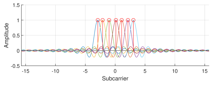
Figure 2.3: OFDM sub-carriers orthogonality.

One of the main advantages introduced by OFDM is the scalability of the rate of transmission: by increasing the transmission period by one symbol, the sub-carriers ‘widen’, causing the bandwidth to increase; vice versa, it decreases by reducing the transmission period. Partially overlapping adjacent sub-carriers can contribute to increasing the bandwidth; this is only feasible because sub-carriers are mathematically orthogonal, hence they do not require an interposed guard band that guarantees non-interference. Moreover, due to sub-carrier orthogonality, possible disturbing interference, noise, and fading phenomena only affect a portion of the sub-carriers, allowing the others to continue their transmission unhindered.

2.3   802.11ax Standard Version

IEEE 802.11ax is associated with Wi-Fi 6 and it operates on the 2.4 and 5 GHz bands, with an additional 6 GHz band in Wi-Fi 6E [23, 24]. Compared to previous versions of the protocol, 802.11ax uses the frequency spectrum more efficiently, thus increasing the overall network throughput and the per-user performance.

The improved performances derive from the implementation — for multi-user communications — of OFDMA, which was already in use in cellular networks since 3GPP LTE but comes as a new approach in Wi-Fi. OFDMA relies on the same structure as OFDM: the available channel is divided into sub-channels, each having its assigned sub-carriers. The user can send their data, split into packets, on a sub-channel for a specific amount of time (or frames), using one or more RU, each one consisting of a set of 26 sub-carriers. An AP can dynamically choose the best RU for each STA it is communicating with, resulting in higher SINR and throughput; OFDMA is also more efficient when the quantity of shared data is limited, as the number of selected RU can vary depending on the sender’s needs.

Compared to previous versions of 802.11, 802.11ax also greatly improves the QOS in crowded environments thanks to Uplink Multi-User MIMO.

The structure of a generic 802.11ax frame respects the following model when implemented in Single-User mode [24]:

[bitheight=1.5bitwidth=0.3]60 20Legacy preamble & 4RL-
SIG 8HE-SIG 4HE-
STF 4HE-
LTF 4HE-
Data 16Packet
Extension

The Legacy preamble guarantees backwards compatibility with previous versions of the 802.11 protocol. The preamble contains information that allows time and frequency synchronization and channel estimation, together with some data regarding payload length and rate of the transmission.

The RL-SIG (Repeated Legacy Signal) field is used to repeat the content of the SIGNAL field of the Legacy preamble.

The rest of the preamble consists of fields that can only be decoded by 802.11ax devices and whose names start with HE (High Efficiency) to distinguish them from the homonymous parameters of the previous versions of the standard. HE-SIG is used to signal the parameters that are needed to correctly decode the rest of the frame (e.g. bandwidth, number of spatial streams, etc.) while HE-STF and HE-LTF are training fields (respectively short and long) used to perform frequency tuning and channel response estimation. The HE-Data field contains the actual user’s data and is followed by a Packet Extension field.

When used in Multi-User mode, the packet structure changes slightly: the HE-SIG field is split into two fields (HE-SIG-A and HE-SIG-B) used to set up and tune MUMIMO transmission.

2.4   802.11be Standard Version

The updated standard is associated with Wi-Fi 7 — released in January 2024, final approval expected by the end of 2024 [25, 26, 27] —, whose key features include [28]:

• MLO;

• Support for 320 MHz-wide channels;

• 4096-QAM modulation scheme;

• Allocation of multiple RU to a single STA;

• Uplink and Downlink single user and multi-user OFDMA and MIMO with up to sixteen spatial streams.

The standard aims to enhance QOS and reduce latency in transmission.

The doubling in the channel’s maximum bandwidth is supported in all Countries that allow the use of Wi-Fi on the 6 GHz band, granting speed in the order of gigabits and higher throughput compared to previous versions of the standard. Moreover, the channel bandwidth can be obtained through the juxtaposition of contiguous and non-contiguous 160+160 MHz bands; an additional bandwidth of 240/160+80 MHz is made available.

The 4096-QAM modulation scheme achieves 20% higher transmission rates than the previously employed 1024-QAM; this improvement contributes to the enhancement of the QOS, combined with the possibility of allocating multiple RU to one STA, which enhances spectral efficiency.

The increased throughput obtained through wider channels, higher order modulation, and MUMIMO allows the transmission rate to reach up to 46 Gbps while maintaining backwards compatibility with previous Wi-Fi standards. An overview of the main differences between 802.11be and 802.11ax is provided in Tab. 2.1.

	Wi-Fi 7 802.11be	Wi-Fi 6E 802.11ax
Launch year	2024	2021
Maximum Throughput	46 Gbps	9.6 Gbps
Frequency Bands	2.4 GHz, 5 GHz, 6 GHz	2.4 GHz, 5 GHz, 6 GHz
Supported Channels	Up to 320/160+160 MHz, 240/160+80 MHz	20, 40, 80, 80+80, 160 MHz
Modulation Scheme	4096-QAM	1024-QAM
MIMO	$16\times 16$ UL/DL MUMIMO	$8\times 8$ UL/DL MUMIMO
RU	Multi-RU	RU

Table 2.1: Main differences between 802.11ax and 802.11be standards [29].

The Wi-Fi standard 802.11be was not used during the experiments carried out in this study; nonetheless, it was deemed important to highlight its main features, as its imminent introduction to the market will soon impact studies on CSI characterization. Analysis of the behaviour of channels up to 160 MHz wide is going to contribute to the study of the 240 and 320 MHz channels newly introduced by 802.11be.

2.5   CSI Structure

CSI can be represented mathematically as a complex number, according to the following formula [30]:

$$\mathbf{C}(n)=||\mathbf{C}(n)||e^{j\angle\mathbf{C}(n)}$$ (2.1)

In this expression, $\mathbf{C}(n)$ is a CSI of the $n$-th sub-carrier, $||\mathbf{C}(n)||$ corresponds to its amplitude and $\angle\mathbf{C}(n)$ to its phase. To maintain consistency with the notation that will be introduced further on, Eq. 2.1 can be rewritten as:

$$\begin{split}\mathbf{C}(k,n)&=A_{\mathbf{C}}(k,n)\cdot e^{j\angle\mathbf{C}(k,n)}\\ &=\sqrt{\Re(\mathbf{C}(k,n))^{2}+\Im(\mathbf{C}(k,n))^{2}}\cdot e^{j\tan^{-1}\left(\frac{\Im(\mathbf{C}(k,n))}{\Re(\mathbf{C}(k,n))}\right)}\end{split}$$ (2.2)

where $\mathbf{C}$ ($k$, $n$) represents the $k$-th CSI of an experiment on the $n$-th sub-carrier and $A_{\mathbf{C}}$ indicates its amplitude.

Amplitude and phase take on different values depending on the properties of the signal at the receiver, according to scattering, reflection, and attenuation of the transmitted signal.

This property of CSI is already evident in a comparison between two basic scenarios, the first (Fig. 2.4) representing CSI collected in an empty room, the second (Fig. 2.5) in the same room with one person sitting at a desk. All CSI plotted in the two figures were collected on channel 157 with 20 MHz bandwidth using 802.11ax; the two experiments were performed at different times of the day, but they both consist of about 18000 CSI collected during 10-minute-long captures. The effect of the AGC was removed from both datasets before plotting.

Figure 2.4: Amplitude CSI collected in an empty room.

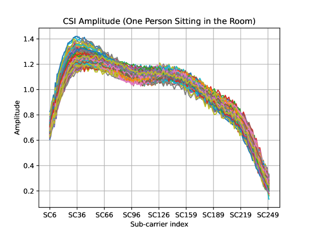
Figure 2.5: Amplitude of CSI collected in a room with one person sitting at a desk.

It immediately comes to the eye that the two plots have different trends, but, more importantly, that the CSI collected in the empty room are more similar to each other compared to those collected in the room with one person, which have a more visible variability. This consideration highlights how the presence of a person — even though they are not moving around — can be detected based on the dispersion of the amplitudes of the CSI. Since the mere presence of a person affects the behavior of the traces, we can expect — and indeed observe in Fig. 2.6 — that the more modifications the environment undergoes, the more variable the corresponding CSI become, reflecting people’s presence and movements in their amplitudes.

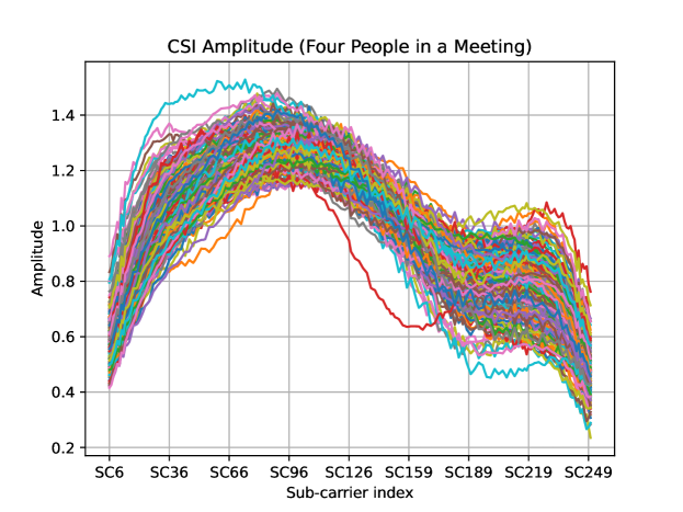
Figure 2.6: Amplitude of CSI collected in a room with four people during a meeting.

This graphical representation of CSI helps to identify the distinction between traces collected in various environments. Since CSI coming from distinct scenarios clearly display different characteristics, we can assume that environment identification based on the collected CSI is feasible. This hypothesis will be thoroughly justified in the discussion carried out in the following chapters.

3     Background and Previous Results

During the BSc Thesis [21], the analysis of CSI traces was mainly focused on the identification of a probability distribution that could be used to describe the increments between consecutive CSI. This chapter serves as a contextualization for the study that is carried out in the following chapters, to provide a uniform background. The results commented in this chapter, as well as some considerations that were already discussed in the previous study, are reported solely for a better understanding of the current work and to make this research self-consistent and comprehensive of all results.

3.1   Data Collection

A relevant difference from the current study is that the data analyzed in [21] consisted of shorter experiments than those performed for this work; specifically, albeit the number of CSI is elevated, the experiments consisted of collections of bursts of CSI with a limited duration (i.e. in the order of tens of seconds) performed in the Telecommunications Laboratory within the Department of Information Engineering at the University of Brescia. Each capture was collected while one person was standing in one of eight fixed spots within the room, with the transmitter and receivers placed along the walls of the laboratory, as can be seen in Fig. 3.1. Moreover, being a preliminary analysis, data categorization was not yet done as described in Chapter 4, therefore the configuration files of the experimental setup are not available.

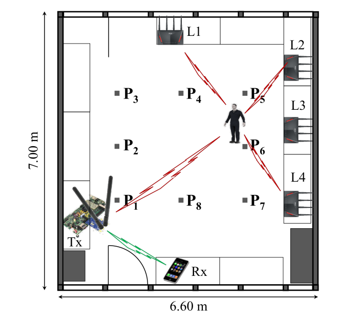
Figure 3.1: Plan of the Telecommunications Laboratory where CSI were collected. Figure taken from [12] with permission by the authors.

No experiments in an empty laboratory were available; nevertheless, comparison between traces collected in different environments and with a varying number of people in the room has only gained relevance in this study, therefore its absence in previous work does not have a meaningful impact.

It must be noted that the impact of AGC was not initially eliminated from the amplitudes, as its removal was introduced in this work, together with normalization and quantization of both increments and amplitudes (see Chapter 6).

3.2   Amplitude Evolution in Time

The initial goal of the study was to identify the presence of correlation in time between the amplitudes on the same sub-carrier. As the first step in the analysis, graphs showing the amplitude evolution in time were presented, with discrete time being the variable on the $x$ axis and amplitude on the $y$ axis. An example of such plots is shown in Fig. 3.2.

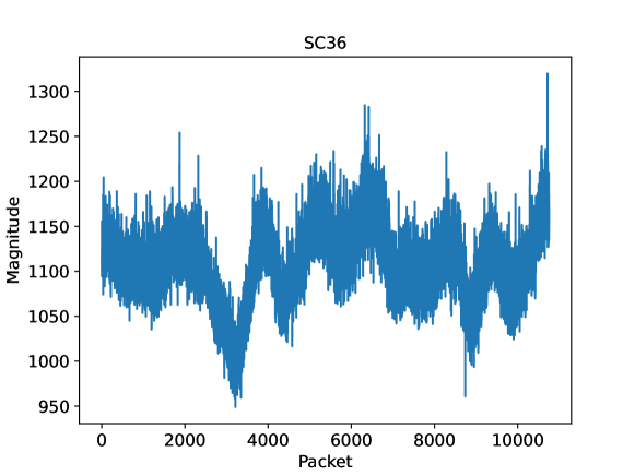
Figure 3.2: Example of amplitude evolution in time on sub-carrier 36. CSI were collected on a 20 MHz bandwidth channel. Image taken from [21].

The fluctuating trend of the CSI is mainly due to the AGC, which undermines considerations about the stationary nature of the process.

It is relevant to specify that multiple features can be identified in various plots showing similar trends on adjacent sub-carriers, which may imply the presence of frequency correlation between the amplitudes.

3.3   Amplitude Relative Frequency Observation

The CSI amplitudes on the different sub-carriers were also shown using histograms having normalized amplitude on the $x$ axis and its relative frequency on the $y$ axis. Fig. 3.3 is an example of the analysis that was carried out.

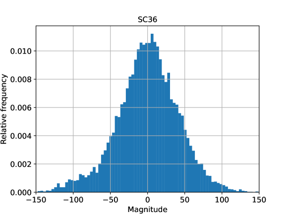
Figure 3.3: Example of amplitude relative frequency on sub-carrier 36. CSI were collected on a 20 MHz bandwidth channel. Image taken from [21].

This approach allowed to make an initial hypothesis about the family of probability distributions that could be used to describe the process of the amplitudes. Nonetheless, the true process that we wanted to characterize was that of the increments, which are the next main topic in the previous research.

3.4   Amplitude Increments and Auto-Correlation

As analysis of the amplitude itself was not deemed sufficient to characterize the evolution of CSI, increments were then taken into account as well by computing their auto-correlation over time on each separate sub-carrier. Their values were assumed to belong to a Markovian process — hence memoryless —, which means that the increments auto-correlation should appear to be noise-like around value 0. This assumption was tested through the empirical evaluation of the auto-correlation of the increments, as shown in Fig. 3.4, which displays a rapid reduction of the values towards zero, as expected. Whether the process can actually be described as Markovian remains to be explored by observing longer experiments performed in different contexts.

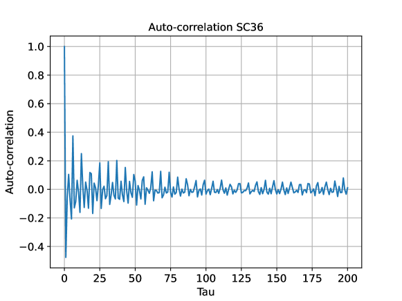
Figure 3.4: Example of increments auto-correlation on sub-carrier 36. CSI were collected on a 20 MHz bandwidth channel. Image taken from [21].

3.5   Amplitude Increments Analysis

The distributions of the increments — see Fig. 3.5 for an example — were compared to a set of known distributions; the Gaussian distribution turned out to be the best-fitting one and was hence chosen as the best approximation and the final proposed model.

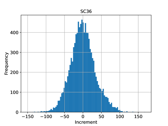
Figure 3.5: Example of increments distribution on sub-carrier 36. CSI were collected on a 20 MHz bandwidth channel. Image taken from [21].

4     Experimental Setup

The collection of all CSI used in the analysis proposed in this thesis was built through multiple separate experiments, with different possible configurations. Two datasets have been analyzed for this work, as described in the following sections.

4.1   Collected data

The main dataset employed in this study was collected within the same office in the Department of Information Engineering at the University of Brescia by Elena Tonini. An approximate layout of the office is provided in Fig. 4.1, which shows the locations of the transmitter and the receiver alongside the main working stations used during office hours.

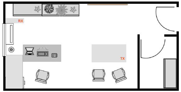
Figure 4.1: Layout of the office where all CSI were collected.

CSI captures were performed in three distinct scenarios:

• Empty Scenario: empty office;

• Static Scenario: one person sitting in the office and working at the desk;

• Fully Dynamic Scenario: multiple people moving around the office.

An additional setup called ‘Dynamic Scenario’ (i.e., one person moving around the office) has been defined and will be taken into account in the future to compare its results with those obtained for the Static and Fully Dynamic scenarios, as it could be considered an intermediate setup between these two.

By associating a json file to each capture, all experiments are categorized according to their own scenario. The file also contains other mandatory fields used to keep track of configuration parameters needed by the hardware itself to set up the data exchange from which CSI are collected; other complementary fields provide corollary information that can be used to fully characterize the experiment. An example of the json configuration file is shown in LABEL:lst:expconfig, while a thorough description of the metadata it contains is provided in App. A.

⬇

1 {

2 "date": {

3 "day": 12,

4 "month": 12,

5 "year": 2023

6 },

7 "locationID": "U004",

8 "experiment": "capture",

9 "adHocTransmission": true,

10 "usleep": 10000,

11 "avgDuration": 600,

12 "bandwidth": 20,

13 "modulation": "ax",

14 "numRx": 1,

15 "numTx": 1,

16 "numAntennasTx": 1,

17 "numAntennasRx": 1,

18 "numSpatialStreams": 1,

19 "people":{

20 "present": true,

21 "num": 2,

22 "moving": false,

23 "names": ["John Smith", "Jane Doe"]

24 },

25 "notes": "JS sitting at the main desk, JD facing him."

26 }

Listing 1: Example of configuration file.

All CSI traces are extracted from OFDM-modulated Wi-Fi frames transmitted over a channel regulated by the 802.11ax protocol. The used channel is number 157 (whose center frequency is 5785 MHz) within the 5 GHz frequency band with 20, 40, and 80 MHz bandwidth.

The traces were extracted using Nexmon Channel State Information Extractor [31, 32]. The analyzed traffic is generated by a board communicating with a receiving device: looking at Fig. 4.1, the transmitter was placed on the bottom right corner of the rightmost desk, whereas the receiver was placed on a rigid support close to the closet on the top left of the room.

The collected data are summarized in Tab. 4.1.

SCENARIO	Empty				Static				Fully Dynamic
802.11	ax				ax				ax
BW (MHz)	20		40	80	20		40	80	20	40				80
# Spatial Streams	1	1	1	1	1	1	1	1	1	1	1	1	1	1	1	1	1
# Experiments	4	5	3	1	4	5	1	1	4	2	1	1	2	2	1	1	1
Avg. Duration (sec.)	600	10	600	600	600	10	600	600	600	600	600	600	600	600	600	600	60
#CSI/exp. (approx.)	18k	300	18k	18k	18k	300	18k	18k	18k	18k	18k	18k	18k	18k	18k	18k	2.6k
# People	0	0	0	0	1	1	1	1	4	2	3	4	5	2	3	4	5

Table 4.1: Summary of the experiments performed for this study. Collected CSI are classified primarily by scenario, additional parameters are then specified as they may vary from one experiment to another.

4.2   Additional available dataset

Some additional collections of CSI have been made available by the authors of [11]. In this work, the data is analyzed to implement CSI obfuscation against unauthorized Wi-Fi sensing, therefore most of it consists of obfuscated traces. Nonetheless, some ‘clean’ collections are available — i.e., retrieved without activating the obfuscator — which are the ones that have been used in this thesis. The goal of studying the channel characterization using data that originates from a different work is to support the sensing techniques implemented in other studies with an innovative approach, leveraging the quantification of the information content of a CSI instead of ML alone.

This dataset was collected on an 80 MHz 802.11ac channel in the Telecommunications Laboratory of the Department of Information Engineering at the University of Brescia in August 2021 by Dr. Marco Cominelli, Prof. Francesco Gringoli, and Prof. Renato Lo Cigno, and it has been used to study device-free localization and test the performance of different obfuscation systems in [11]. From this point onward, the dataset will be referred to as the ‘AntiSense dataset’. Its content is relative to CSI captured with the same person standing in one of 8 pre-determined target positions and with a receiver placed in one of 5 fixed spots just outside the perimeter of the laboratory, as displayed in Fig. 4.2.

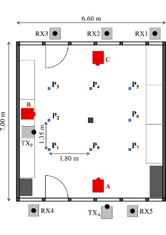
Figure 4.2: Plan of the lab where the AntiSense dataset was collected. The blue squares represent the eight possible locations of the person within the room; the red boxes labelled A, B, and C are the locations of the obfuscator in different scenarios: for the scope of this work, their effect is irrelevant; the transmitter inside the room is used for passive attacks, the one outside is used for active ones. Figure taken from [11] with permission by the authors.

The transmitter was placed either on the left wall of the laboratory or just outside the door at the bottom of Fig. 4.2, depending on the experiment. In our study, we will only focus on the CSI collected when the active transmitter was that outside of the laboratory. The technology used to extract the CSI is the same as that described in Sect. 4.1.

For each of the two positions of the transmitter, the dataset has then been partitioned into a training, a testing, and a validation dataset, each consisting of eight captures for each position the receiver was placed in. For the scope of this work, only the training and testing datasets will be analyzed. As a whole, the dataset employed in this study consists of 120 captures, 40 of which are discarded (the validation partition), divided as shown in Tab. 4.2.

PARTITION		TRAINING					TESTING					VALIDATION
RX POS.		rx1	rx2	rx3	rx4	rx5	rx1	rx2	rx3	rx4	rx5	rx1	rx2	rx3	rx4	rx5
	P1	1000	1000	1000	1000	1000	1000	1000	1000	1000	1000	200	200	200	200	200
	P2	1000	1000	1000	1000	1000	1000	1000	1000	1000	1000	200	200	200	200	200
	P3	1000	1000	1000	1000	1000	1000	1000	1000	1000	1000	200	200	200	200	200
	P4	1000	1000	1000	1000	1000	1000	1000	1000	1000	1000	200	200	200	200	200
	P5	1000	1000	1000	1000	1000	1000	1000	1000	1000	1000	200	200	200	200	200
	P6	1000	1000	1000	1000	1000	1000	1000	1000	1000	1000	200	200	200	200	200
	P7	1000	1000	1000	1000	1000	1000	1000	1000	1000	1000	200	200	200	200	200
POS. OF PERSON IN THE ROOM	P8	1000	1000	1000	1000	1000	1000	1000	1000	1000	1000	200	200	200	200	200
TOT. CSI		8000	8000	8000	8000	8000	8000	8000	8000	8000	8000	1600	1600	1600	1600	1600

Table 4.2: Summary of the experiments making up the AntiSense dataset. Collected CSI are classified according to the dataset partition they belong to, the position of the receiver and that of the person in the room. P1 through P8 reference the positions displayed in Fig. 4.2.

5     Notation

Let $\mathbf{C}(k,n)$ be the CSI collected during a generic experiment; $k\in[1,M_{\mathbf{C}}]$ is the sequence number (ordering) of the collection, which consists of $M_{\mathbf{C}}$ samples, and $n\in[1,N_{\text{\tiny SC}}]$ is the index of the sub-carrier. $N_{\text{\tiny SC}}$ is the number of useful sub-carriers, i.e., those that are not suppressed in transmission and can be usefully employed to estimate the CSI. $\mathbf{C}(k,n)$ is a bi-dimensional vector containing the I/Q samples of the CSI, represented as a complex number with real and imaginary parts, so that

$$A_{\mathbf{C}}(k,n)=\sqrt{\Re(\mathbf{C}(k,n))^{2}+\Im(\mathbf{C}(k,n))^{2}}$$

is the amplitude of $\mathbf{C}(k,n)$.

The total collection of the samples of an experiment $\mathbf{C}(\cdot,\cdot)$ can be (and normally is) annotated with additional data such as the descriptor of the experiment, the sub-carrier spacing, and so forth, as described in Chapter 4, while each sample $\mathbf{C}(k,\cdot)$ is annotated at least with the absolute time $\delta t_{k}=t_{r}[\mathbf{C}(k,\cdot)]-t_{r}[\mathbf{C}(k-1,\cdot)]$, where $t_{r}(\cdot)$ is a function measuring the actual reception time of the frame with the collected CSI. Clearly, $\delta t_{0}=\text{NaN}$ is undefined and irrelevant.

Tab. 5.1 summarizes relevant symbols, including those that have not been introduced yet in this chapter as they will be encountered further on in the discussion.

SYMBOL	DESCRIPTION
$\mathbf{C}(k,n)$	CSI collected during a generic experiment
$k\in[1,M_{\mathbf{C}}]$	Sequence number of a CSI within the collection
$M_{\mathbf{C}}$	Number of samples of the collection
$n\in[1,N_{\text{\tiny SC}}]$	Index of the sub-carrier
$N_{\text{\tiny SC}}$	Number of useful sub-carriers
$A_{\mathbf{C}}(k,n)$	Amplitude of $\mathbf{C}(k,n)$
$\delta t_{k}$	Absolute time of $\mathbf{C}(k,n)$
$t_{r}(\cdot)$	Reception time of the frame with the collected CSI
$\overline{A_{\mathbf{C}}}$	Energy of a CSI
$A_{\mathbf{C}}^{\min}$	Minimum amplitude value across all CSI
$A_{\mathbf{C}}^{\max}$	Maximum amplitude value across all CSI
$A^{\star}_{\mathbf{C}}(n)$	Reference CSI computed on each experiment
$\delta_{\mathbf{C}}(k,n)$	Increment between two CSI on the same sub-carrier $n$
$\delta_{\mathbf{C}}^{\min}$	Minimum increment value across all CSI
$\delta_{\mathbf{C}}^{\max}$	Maximum increment value across all CSI
$\mathcal{N}(\sigma)$	Gaussian distribution with standard deviation $\sigma$
$\mathcal{N^{\prime}}(\sigma)$	Quantized Gaussian distribution with standard deviation $\sigma$
$q_{\text{\tiny inc}}$	Number of bits used to quantize the increments
$q_{\text{\tiny amp}}$	Number of bits used to quantize the amplitude
$P_{w}$	Probability weight of the tails of $\mathcal{N}$
$\delta^{\star}$	Value of the increments after which tails are discarded
$I(X;Y)$	Mutual information between random variables $X$ and $Y$
$\mathcal{I}_{A}$	Internal MI for experiment $A$
$\mathcal{E}_{A,B}$	External MI between experiment $A$ and $B$
$\text{WHD}(A^{\star}_{\mathbf{C}},A_{\mathbf{C}}(k,\cdot))$	Weighted Hamming Distance between $A^{\star}_{\mathbf{C}}$ and $A_{\mathbf{C}}$
$\overline{\text{WHD}(A^{\star}_{\mathbf{C}},A_{\mathbf{C}})}$	Average WHD between $A^{\star}_{\mathbf{C}}$ and $A_{\mathbf{C}}$

Table 5.1: Summary of the used symbols, in order of appearance.

6     Normalization and Quantization

Before delving into the processing and analysis of the collected data, it is necessary to introduce a standard representation of $A_{\mathbf{C}}(k,n)$ to ensure the feasibility of the comparisons between different experiments. The following processing is done separately on each experiment.

The first step in the conditioning of the collected data is the normalization of the CSI amplitude in the assumption that the transmitted energy is constant, as it should be, and variations in the collected data are due only to different gains of the AGC at the receiver:

$$\overline{A_{\mathbf{C}}}=\frac{1}{N_{\text{\tiny SC}}}\sum_{n=1}^{N_{\text{\tiny SC}}}A_{\mathbf{C}}(k,n);\quad A_{\mathbf{C}}(k,n)=\frac{A_{\mathbf{C}}(k,n)}{\overline{A_{\mathbf{C}}}}\forall n\in[1,N_{\text{\tiny SC}}]$$ (6.1)

Next, all values are mapped in the $[0,1]$ interval as follows. First, the minimum amplitude value is computed and subtracted from all values across all CSI and sub-carriers:

$$A_{\mathbf{C}}^{\min}=\min_{k\in[1,M_{\mathbf{C}}],n\in[1,N_{\text{\tiny SC}}]}A_{\mathbf{C}}(k,n)$$ (6.2)

$$A_{\mathbf{C}}(k,n)=A_{\mathbf{C}}(k,n)-A_{\mathbf{C}}^{\min},\,k\in[1,M_{\mathbf{C}}],n\in[1,N_{\text{\tiny SC}}]$$ (6.3)

Next, the maximum is computed; this is in practice the maximum difference between the minimum and the maximum of the original sequence. Its value is employed to normalize the amplitude to one:

$$A_{\mathbf{C}}^{\max}=\max_{k\in[1,M_{\mathbf{C}}],n\in[1,N_{\text{\tiny SC}}]}A_{\mathbf{C}}(k,n)$$ (6.4)

$$A_{\mathbf{C}}(k,n)=\frac{A_{\mathbf{C}}(k,n)}{A_{\mathbf{C}}^{\max}},\,k\in[1,M_{\mathbf{C}}],n\in[1,N_{\text{\tiny SC}}]$$ (6.5)

Since the minimum and maximum amplitude values are computed over the whole experiment rather than referring to a single trace, it is possible for some CSI to not fully cover the interval from 0 to 1. Hence, some traces may not reach the limits of the normalization interval at all, but, over the entire experiment, there will be at least one CSI that is equal to 0 — and, similarly, to 1 — on at least one sub-carrier. The CSI taking on these two values may be distinct traces.

Finally, a reference CSI amplitude is calculated for each experiment as the average over $k\in[1,M_{\mathbf{C}}]$ of all the CSI collected during the experiment:

$$A^{\star}_{\mathbf{C}}(n)=\frac{1}{M_{\mathbf{C}}}\sum_{k=1}^{M_{\mathbf{C}}}A_{\mathbf{C}}(k,n)$$ (6.6)

This reference CSI is taken as the representative of the experiment to estimate the information content embedded in the CSI by the propagation environment in the different experiments.

6.1   Estimate of the Increments Process

Once the amplitude of the CSI is properly normalized, the process of the increments can be estimated. An increment in amplitude is defined as the difference between the values of the amplitude of two different (not necessarily consecutive) CSI on the same sub-carrier. Mathematically:

$$\delta_{\mathbf{C}}(k,n)=A_{\mathbf{C}}(k+\delta t,n)-A_{\mathbf{C}}(k,n)$$ (6.7)

This topic has been analyzed more in-depth in [21], whose goal is to provide a simple mathematical model that can be used to approximate the process of the increments on each sub-carrier. The work suggests that — at least in an initial approach to the process estimation — it is possible and sufficient to use a Normal distribution to approximate the process on each sub-carrier. Through the properties of Gaussian distributions, it is possible to combine the Normal distribution of each sub-carrier to create a single Gaussian distribution $\mathcal{N}(\sigma)$ that can be used to represent the entire process of the increments across all sub-carriers used during transmission. In this process, the average is zero by construction, but it must be zero also because an increment process with non-zero mean implies a non-stationary process on the one hand, and, on the other hand, either a diverging received — and transmitted — power or a vanishing signal, and both cases are not meaningful in this work.

In other words, this work assumes that all increments of each element $A_{\mathbf{C}}(k,n)$ of the CSI are i.i.d..

Given these assumptions, a stochastic model of the CSI amplitude evolution is:

$$A_{\mathbf{C}}(k,n)=A_{\mathbf{C}}(k-1,n)+\mathcal{N}(\sigma),\,k\in[2,M_{\mathbf{C}}],n\in[1,N_{\text{\tiny SC}}],$$ (6.8)

thus there is only the need to estimate $\sigma$ given all the available increment samples $\delta_{\mathbf{C}}(k,n)=A_{\mathbf{C}}(k,n)-A_{\mathbf{C}}(k-1,n),\,k\in[2,M_{\mathbf{C}}],n\in[1,N_{\text{\tiny SC}}]$. To avoid cluttering the notation, $\sigma$ and its estimate are indicated with the same symbol:

$$\sigma=\frac{1}{N_{\text{\tiny SC}}}\sum_{n=1}^{N_{\text{\tiny SC}}}\left[\frac{1}{M_{\mathbf{C}}-1}\sqrt{\sum_{k=2}^{M_{\mathbf{C}}}\delta_{\mathbf{C}}^{2}(k,n)}\right]$$ (6.9)

Indeed, $\sigma$ can be estimated differently, as the evolution of $A_{\mathbf{C}}(k,n)$ has memory. In a process with memory, Eq. 6.9 correctly estimates the one-step increment marginal distribution, but may not represent the n-step increment marginal distribution correctly, as well known, as memory may even eventually make processes self-similar. Although this discussion will not be brought on further, note that $\sigma$ can be estimated as:

$$\sigma=\frac{1}{N_{\text{\tiny SC}}}\sum_{n=1}^{N_{\text{\tiny SC}}}\left[\frac{1}{M_{\mathbf{C}{T}}-1}\sqrt{\sum_{h}^{M_{\mathbf{C}{T}}}\delta{h}_{\mathbf{C}}^{2}(k,n)}\right]$$ (6.10)

where

$$M_{\mathbf{C}{T}}=(M_{\mathbf{C}}-1)+(M_{\mathbf{C}}-2)+\cdots+(M_{\mathbf{C}}-\left\lfloor\frac{M_{\mathbf{C}}}{2}\right\rfloor)$$

and $\delta{h}_{\mathbf{C}}=A_{\mathbf{C}}(k,n)-A_{\mathbf{C}}(k-h,n),\,k\in[2,M_{\mathbf{C}}-h+1],n\in[1,N_{\text{\tiny SC}}]$. The n-step increments are limited to $\left\lfloor\frac{M_{\mathbf{C}}}{2}\right\rfloor$ to have enough samples for each increment gap. This latter estimate should yield a larger variance of the process as normally $\delta{h}_{\mathbf{C}}>\delta_{\mathbf{C}}$ for $h\geq 2$. Which estimate is better and hence chosen will be decided based on the effectiveness of the modelling in predicting the information content of experiments.

6.2   Quantization and Mapping

Amplitude $A_{\mathbf{C}}(\cdot,\cdot)$ needs to be quantized for two reasons. First and foremost, working with real numbers makes estimating information content (in the sense of Shannon theory) of CSI extremely difficult. Second, indeed, the measure of the CSI itself is already quantized by the hardware that collects it but, unfortunately, access to the low-level measures is not given. The hardware exports $A_{\mathbf{C}}$ values in floating point format, so knowing the exact representation of $\mathbf{C}(\cdot,\cdot)$ is impossible and, in any case, the pre-processing described so far is best done using floating point. Since both $A_{\mathbf{C}}$ and $\delta_{\mathbf{C}}$ values need to be quantized to provide a correct and comprehensive representation of the collected data, this section will start with the approach to quantization of $\delta_{\mathbf{C}}$ values.

Before quantizing the increments, it is necessary to apply the same procedure used on the amplitudes to ensure that $\delta_{\mathbf{C}}(k,n)\in[0,1]$. Firstly, we compute the minimum value of the increments:

$$\delta_{\mathbf{C}}^{\min}=\min_{k\in[1,M_{\mathbf{C}}],n\in[1,N_{\text{\tiny SC}}]}\delta_{\mathbf{C}}(k,n)$$ (6.11)

$$\delta_{\mathbf{C}}(k,n)=\delta_{\mathbf{C}}(k,n)-\delta_{\mathbf{C}}^{\min},\,k\in[1,M_{\mathbf{C}}],n\in[1,N_{\text{\tiny SC}}]$$ (6.12)

Next, compute the maximum and normalize the increments to one:

$$\delta_{\mathbf{C}}^{\max}=\max_{k\in[1,M_{\mathbf{C}}],n\in[1,N_{\text{\tiny SC}}]}\delta_{\mathbf{C}}(k,n)$$ (6.13)

$$\delta_{\mathbf{C}}(k,n)=\frac{\delta_{\mathbf{C}}(k,n)}{\delta_{\mathbf{C}}^{\max}},\,k\in[1,M_{\mathbf{C}}],n\in[1,N_{\text{\tiny SC}}]$$ (6.14)

The approach to increment normalization is clearly the same as that used with amplitudes, as shown by Eq. 6.2 to Eq. 6.5.

For the reasons mentioned at the beginning of this section, the quantization process of the increments is based on some simple reasoning: the number of used bits should be the smallest possible to represent the increments reasonably accurately; in other words, the PDF of $\mathcal{N}(\sigma)$ should be reasonably approximated by the PMF of $\mathcal{N^{\prime}}(\sigma)$, where $\mathcal{N^{\prime}}(\sigma)$ is the quantized version of $\mathcal{N}(\sigma)$; notice that there is no need to quantize $\sigma$, but only the output of the distribution (whether it is used as a random generator of synthetic $\delta_{\mathbf{C}}$ values or empirically built on experimental data).

There are many ways of defining a good approximation, both in terms of residual errors and in probabilistic terms. Let us, for the time being, neglect this specific step and assume that $q_{\text{\tiny inc}}$ bits are used to represent $\mathcal{N^{\prime}}(\sigma)$, or, equivalently, the quantized version of $\delta_{\mathbf{C}}(k,n)$.

First of all, a maximum (and minimum) value of $\mathcal{N}(\sigma)$ needs to be set. This helps to define a symmetrical and finite interval of values that $\mathcal{N}$ can be defined on, essentially cutting off the tails of the distribution that would make its domain infinite and hard to work with. This is easily done by defining the probability weight $P_{w}$ of the tails that are thus discarded and selecting an appropriate value. The reference equation is:

$$P_{w}=\frac{2\sigma}{\sqrt{\pi}}\int_{\delta^{\star}}^{\infty}\mathcal{N}(\sigma)d\delta$$ (6.15)

To properly select $\delta^{\star}$ given a desired $P_{w}$, error function tables or calculators can be used. To maintain discussion and implementation simple, $\delta^{\star}$ is set to a value that is an integer multiple of the standard deviation of the Normal distribution; specifically, $\delta^{\star}=n\sigma$ with $n$ integer such that Eq. 6.15 is smaller than the desired probability. This probability can be selected simply by observing that, given a certain number of collected samples, probabilities smaller than the inverse of the number itself cannot be estimated. Therefore, in this case, selecting $\frac{1}{N_{\text{\tiny SC}}}<P_{w}<\frac{10}{N_{\text{\tiny SC}}}$ is appropriate.

For reasons that will become clear later in the discussion, $q_{\text{\tiny inc}}$ can be selected such that $\mathcal{N^{\prime}}(\sigma)$ is centred around zero (obvious) and its support is over 7, 15, or 31 values only. As $q_{\text{\tiny inc}}$ bits are used to represent the entire interval $[0,1]$ with uniform quantization, $q_{\text{\tiny inc}}$ selection as a function of $\delta^{\star}$ and the cardinality of $\mathcal{N^{\prime}}(\sigma)$ support is straightforward. Indeed, there are boundary conditions to be fixed in the numerical computation as $\delta^{\star}$ may not be coincident with any sampling interval and $\mathcal{N^{\prime}}(\sigma)$ must be normalized to be a proper distribution, i.e., the weight $P_{w}$ must be accounted for.

A simple and effective way of fixing the boundary conditions is to approximate $\delta^{\star}$ with the nearest sampling interval larger than $\delta^{\star}$ and accumulate $P_{w}$ on the boundary intervals. This is a good approximation method as long as the probabilities that are accumulated on the boundary intervals do not alter the structure of the Normal distribution, i.e. as long as they do not increase the probability of the outermost intervals to the point that the resulting distribution no longer resembles a Normal distribution.

By leveraging the boundary conditions — and therefore limiting the domain of $\mathcal{N^{\prime}}(\sigma)$ to $[-\delta^{\star},\delta^{\star}]$ — symmetry of $\mathcal{N^{\prime}}$ around zero is ensured.

Up to this point, only quantization of the distribution of the increments has been taken into account, but $A_{\mathbf{C}}$ needs to be quantized as well. This will allow to finally switch to work with integer, finite numbers representing both the absolute amplitude values and the increments of the CSI coherently. Coherent representation means that the quantization interval of both $\mathcal{N}$ and $A_{\mathbf{C}}$ must be the same, which implies that the number of bits used to quantize $\mathcal{N}$ is smaller than the number of bits used to represent $A_{\mathbf{C}}$.

Switching to this representation, a CSI is a vector of integer positive numbers of dimension $N_{\text{\tiny SC}}$. The generation of a synthetic trace of $A_{\mathbf{C}}$ values — that is, a new CSI — is obtained by adding a vector of increments ($\delta_{\mathbf{C}}$) with the same dimension to generate a new CSI; iterating the procedure produces new CSI. To be able to add $\delta_{\mathbf{C}}$ to $A_{\mathbf{C}}(k,n)$ we have to make sure that the quantization process uses the same quantization interval for increments and amplitudes, which may require the introduction of some tricks to obtain a coherent and consistent result.

Forcing the quantization intervals of the increments and the amplitudes to be exactly the same is not easy because $\delta^{\star}$ is not necessarily equal to $k\cdot 2^{-n}$ with $k,n\in\mathbb{N}$. Therefore, we first have to set the number of quantization bits of $A_{\mathbf{C}}$ to

$$q_{\text{\tiny amp}}=\left\lceil\log_{2}\left(\frac{1}{\delta^{\star}}\times(2^{q_{\text{\tiny inc}}}+1)\right)\right\rceil$$ (6.16)

where $q_{\text{\tiny inc}}$ is the number of bits used to quantize $\delta_{\mathbf{C}}$. Next, we have to ‘tune’ $\delta^{\star}$ on the first sampling interval boundary larger than $\delta^{\star}$ and re-sample the increments. From now on $\delta^{\star}$ refers to the tuned version, so that $A_{\mathbf{C}}$ and $\delta_{\mathbf{C}}$ are sampled with exactly the same sampling interval and each value of $\mathcal{N^{\prime}}(\sigma)$ has the appropriate probability value. It is important to note that in a generative process all of this will be done before generating increments.

With this approach, the study is not strictly bound to use Normal distributions and it is also possible to compute a quantized empirical distribution starting from measured values.

This approach ensures that both quantities are defined and quantized over the same interval and using the appropriate numbers of bits, allowing easy and correct summation of $A_{\mathbf{C}}$ and $\delta_{\mathbf{C}}$ values. Since a CSI normalized between 0 and 1 may not reach the ends of the normalization interval, as said in the paragraph following Eq. 6.5, the quantized CSI are naturally subject to the same consideration. Therefore, the generic quantized CSI may not be equal to 0 or $2^{q_{\text{\tiny amp}}}-1$ on any sub-carrier, but at least one CSI within each experiment will reach such values on at least one sub-carrier.

Again, to avoid cluttering the notation, from now on we will assume that all the quantities have been correctly quantized and mapped; the same symbols ($A_{\mathbf{C}}$, $\delta_{\mathbf{C}}$, $\mathcal{N}$, …) introduced so far will be used to represent the quantized version of the variables.

6.3   Visualization of the Normalization and Quantization Processes

To support the understanding of the normalization and quantization processes, a visual representation of the variations that amplitudes undergo is shown in the following paragraphs. Two examples of randomly chosen CSI are selected: the first, displayed on the left column of Fig. 6.1, belongs to a ten-minute-long experiment performed in the Empty Scenario, and the second (right column) comes from an equally long experiment performed in the Static Scenario. Both setups are described in Chapter 4. The original amplitude values indicated on the $y$-axis in Fig. 6.1(a), 3 and 6.1(b) are arbitrary values detected by the receiver, therefore the measurement has no reference scale. This consideration is at the base of the whole normalization and quantization processes, as without such processing the comparison of different CSI would be harder to carry out.

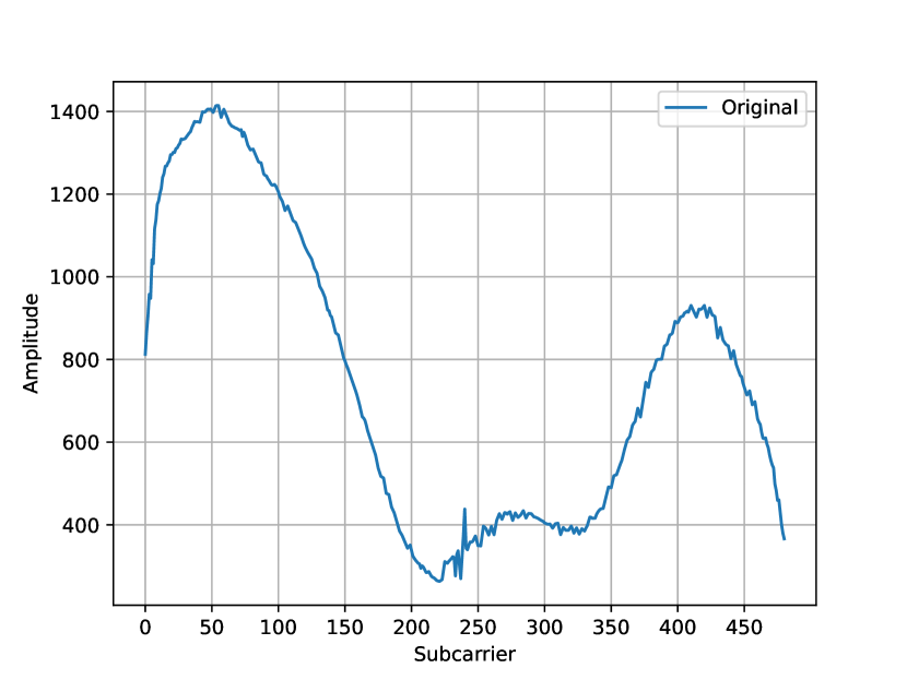
(a) Original CSI amplitude

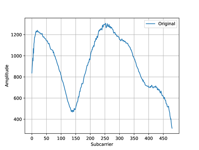
(b) Original CSI amplitude

(c) Removed impact of AGC as per Eq. 6.1

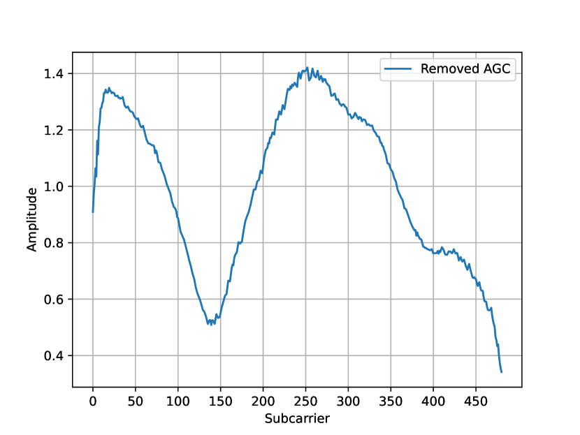
(d) Removed impact of AGC as per Eq. 6.1

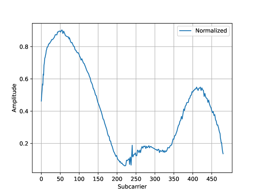
(e) Normalized

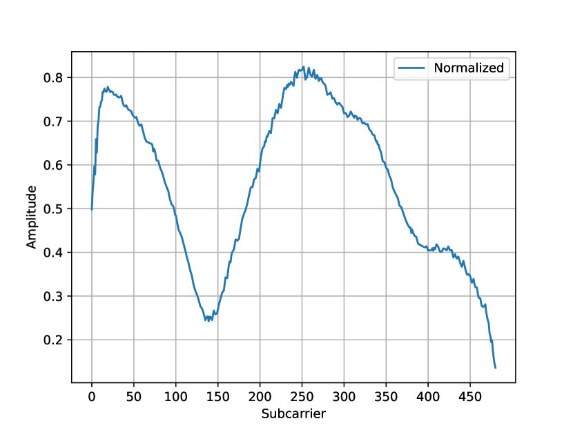
(f) Normalized

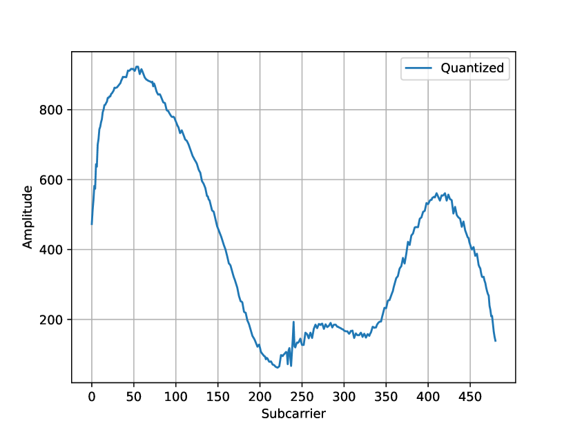
(g) Quantized

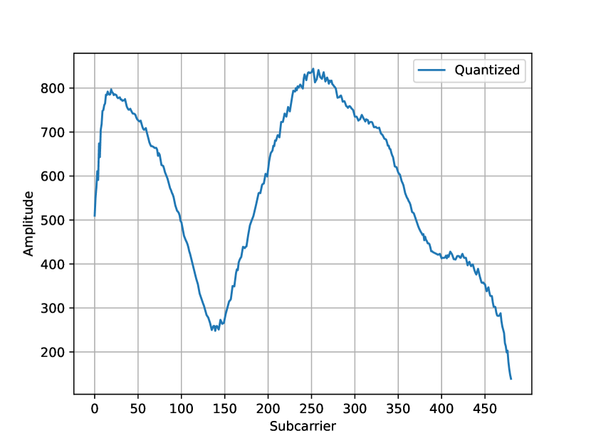
(h) Quantized

Figure 6.1: Visualization of the numerical processing on the CSI in the Empty (left) and Static (right) Scenarios. Data collected on a 40 MHz bandwidth channel using 802.11ax.

The relevant feature that comes across by looking at Fig. 6.1 is that the structure of the CSI remains unaltered after each step of elaboration. The changing element of the displayed plots is the scale on the $y$ axis, as the value of the amplitude is scaled on different intervals. Specifically, the mitigation of the effects of AGC through the normalization with respect to the energy of the CSI (Eq. 6.1) brings the amplitude values closer to 1, which is then set as the maximum value by the normalization described through Eq. 6.2 to Eq. 6.5.

As already highlighted in the comments to Eq. 6.5, it is possible that some CSI across the experiment do not reach the values 0 and 1 (i.e., both ends of the normalization range) because the normalization is done using the maximum amplitude reached during the whole experiment, rather than that of the individual CSI. The traces displayed in Fig. 6.1 are an example of this behavior.

The amplitudes in the $[0,1]$ interval are then mapped onto the $[0,2^{q_{\text{\tiny amp}}}-1]$ interval through quantization. Moreover, it is also evident that the CSI collected in the Static scenario (i.e., with one person in the room sitting at the desk while working on a laptop) differs from the one collected in the empty room, highlighting how CSI directly reflect the properties of the environment in the changes of their amplitude structure.

7     Mutual Shannon Information

The MI between two random variables is a measure of the mutual dependence of the two variables. In terms of PMF for discrete distributions, the MI between two discrete random variables $X$ and $Y$ is computed as a double sum:

$$\begin{split}I(X;Y)&=\sum_{y\in\mathcal{Y}}\sum_{x\in\mathcal{X}}P_{(X,Y)}(x,y)\log\left(\frac{P_{(X,Y)}(x,y)}{P_{X}(x)P_{Y}(y)}\right)\\ &=\sum_{y\in\mathcal{Y}}\sum_{x\in\mathcal{X}}P(x|y)\cdot P_{Y}(y)\log\left(\frac{P(x|y)\cdot P_{Y}(y)}{P_{X}(x)P_{Y}(y)}\right)\\ &=\sum_{y\in\mathcal{Y}}\sum_{x\in\mathcal{X}}P(x|y)\cdot P_{Y}(y)\log\left(\frac{P(x|y)}{P_{X}(x)}\right)\end{split}$$ (7.1)

where $P_{(X,Y)}$ is the joint probability mass function of $X$ and $Y$ and $P_{X}$ and $P_{Y}$ are the marginal probability functions of $X$ and $Y$ respectively. In terms of PDF for continuous distributions, the sums in the formula are exchanged for integrals, allowing integration in $dx$ and $dy$ respectively.

MI essentially measures how knowledge of the probability of an event impacts knowledge about the other. In the analysis of CSI, MI represents the amount of information that a reference CSI $A^{\star}_{\mathbf{C}}$ provides about another CSI $A_{\mathbf{C}}$ or vice versa. If $X$ and $Y$ are two disjoint discrete random variables, knowing anything about either of them provides no additional information about the other variable. Contrarily, if the value of $X$ can be deterministically calculated based on that of $Y$, the MI is the same as the uncertainty about either of the two variables’ values (i.e., the entropy of $X$ or $Y$).

Some relevant properties of the MI are:

• $I(X;Y)=0\Leftrightarrow X$ and $Y$ are independent random variables. This is due to the fact that $p_{(X,Y)}(x,y)=p_{X}(x)\cdot p_{Y}(y)$, causing the content of the logarithm function to be equal to 1, meaning that $\log\left(\frac{p_{(X,Y)}(x,y)}{p_{X}(x)p_{Y}(y)}\right)=\log(1)=0$;

• Non-negativity: $I(X;Y)\geq 0$;

• Symmetry: $I(X;Y)=I(Y;X)$.

Note that the non-negativity holds when $\left(\frac{P(x|y)\cdot P_{Y}(y)}{P_{X}(x)P_{Y}(y)}\right)=0$ and $log(0)$ is undefined by leveraging the properties of infinitesimal calculus: in such condition, in fact, $P(x|y)$ is what causes the argument of the logarithm to be zero, but this value also multiplies the logarithm, making it unnecessary to compute the product between their finite values as it will always be equal to zero regardless of the resulting logarithm.

MI can alternatively be computed as a function of entropy and conditional entropy:

$$\begin{split}I(X;Y)&\equiv H(X)-H(X|Y)\\ &\equiv H(Y)-H(Y|X)\\ &\equiv H(X)+H(Y)-H(X,Y)\\ &\equiv H(X,Y)-H(X|Y)-H(Y|X)\end{split}$$ (7.2)

where $H(X)$ represents the entropy of $X$, $H(X|Y)$ represents the conditional entropy of $X$ given the knowledge about $Y$, and $H(X,Y)$ is the joint entropy of $X$ and $Y$.

The application of the MI equation in this study works as a quantitative measurement to determine whether two CSI belong to the same experiment, assuming that two CSI coming from different captures (i.e., different locations, number of people in the room, etc.) bear little additional information about each other, whereas two samples belonging to the same experiment have a higher MI value. Numerically, we assume that samples belonging to experiments performed in distinct environments have a MI value closer to (or equal to, in case of complete independence) zero, whereas samples coming from experiments performed with the same setup have a value asymptotically growing to infinity. To represent an infinite value using a finite set of numbers, an upper limit is set to the value of the MI.

The analysis can start by computing the MI between the value taken by the average CSI $A^{\star}_{\mathbf{C}}$ — which is representative of the whole experiment — and that of another CSI $A_{\mathbf{C}}(k,n)$ on a chosen sub-carrier $n\in[0,N_{\text{\tiny SC}}]$, with any $k\in[1,M_{\mathbf{C}}]$. To derive each $A_{\mathbf{C}}(k,n)$, an increment $\delta_{\mathbf{C}}$ is added to $A_{\mathbf{C}}(k-1,n)$, with $\delta_{\mathbf{C}}$ belonging to a known discrete probability distribution that can be modelled as a quantized Gaussian distribution (according to the quantization process described in Chapter 6). This characterization of the increments as belonging to a Normal distribution simplifies the computation of the probabilities of an increment $\delta_{\mathbf{C}}$ being added to $A_{\mathbf{C}}(k-1,n)$ and that of $\delta_{\mathbf{C}}$ occurring at all. From now on we will consider $A_{\mathbf{C}}(k-1,n)=A^{\star}_{\mathbf{C}}(n)$ to compute the MI between the reference CSI and another one from the same capture.

Once $k\in[1,M_{\mathbf{C}}]$ is defined as the index of the CSI to consider within the experiment and $n\in[0,N_{\text{\tiny SC}}]$ is chosen as the analyzed sub-carrier, the computation of the MI requires knowing some probability values, such as:

• $P(A_{\mathbf{C}}(k,n)|A^{\star}_{\mathbf{C}}(n))$: it can be computed as the probability of drawing a specific $\delta_{\mathbf{C}}$ value from the quantized Normal distribution and obtaining $A_{\mathbf{C}}(k,n)$ by adding the increment $\delta_{\mathbf{C}}$ to $A^{\star}_{\mathbf{C}}(n)$. Essentially, it is equal to $P[\delta_{\mathbf{C}}:A^{\star}_{\mathbf{C}}(n)+\delta_{\mathbf{C}}==A_{\mathbf{C}}(k,n)]$;

• $P(A_{\mathbf{C}}(k,n))$

• $P(A^{\star}_{\mathbf{C}}(n))$

Computing these probabilities allows to calculate the MI between two amplitude values at consecutive time steps on a fixed sub-carrier.

Given that the goal is to compute the MI between CSI as a whole and not on each sub-carrier by itself, a value to represent the probability of an entire CSI $\mathbf{C}(k)$ happening in an experiment is also needed. Assuming, as a simplification, that all sub-carriers are independent, this is given by:

$$P(\mathbf{C}(k))=\prod_{n\in[0,N_{\text{\tiny SC}}]}P(A_{\mathbf{C}}(k,n))$$ (7.3)

Considering that an analysis that only looks at MI sub-carrier by sub-carrier would be too limited and that it would not return the actual MI between CSI, it becomes necessary to translate what has been described in this chapter up to this point to work with CSI as a whole rather than splitting them $N_{\text{\tiny SC}}$ times.

We can, at this point, consider the amplitudes of the CSI $A_{\mathbf{C}}$ across the $N_{\text{\tiny SC}}$ sub-carriers as symbols of an alphabet. The alphabet is very large, but finite, having $2^{(N_{\text{\tiny SC}}\cdot q_{\text{\tiny amp}})}$ symbols, hence MI is always finite and numerical evaluations can proceed, albeit with care to avoid numerical problems in case of very large (or very small) numbers.

First of all, Eq. 7.3 can be extended as follows:

$$\begin{split}P(\mathbf{C}(k))&=\prod_{n\in[0,N_{\text{\tiny SC}}]}P(A_{\mathbf{C}}(k,n))\\ &=\prod_{n\in[0,N_{\text{\tiny SC}}]}\frac{1}{2^{q_{\text{\tiny amp}}}}\\ &=\frac{1}{2^{N_{\text{\tiny SC}}\cdot q_{\text{\tiny amp}}}}\end{split}$$ (7.4)

This implies that — ignoring cross-sub-carrier dependence — any CSI $\mathbf{C}(k)$ has the same probability of happening, given the available alphabet. Unfortunately, it is clear that, given any reasonable $N_{\text{\tiny SC}}$ and $q_{\text{\tiny amp}}$, $\frac{1}{2^{N_{\text{\tiny SC}}\cdot q_{\text{\tiny amp}}}}$ is way too small to allow any numerical evaluation of Eq. 7.1 or derivations thereof without further manipulation or approximation.

One possible, quick solution is to use a polynomial expansion of the logarithm and exploit the fact that $P(\mathbf{C}(k))$ is constant. One possibility is to use the bilinear expansion:

$$\log(x)=2\left[\left(\frac{x-1}{x+1}\right)+\frac{1}{3}\left(\frac{x-1}{x+1}\right)^{3}+\frac{1}{5}\left(\frac{x-1}{x+1}\right)^{5}+\ldots\right]$$ (7.5)

An alternative method to approximate the logarithm could be the following: it is known that

$$\log(x)-\log(1)=(x-1)-\frac{(x-1)^{2}}{2}+\frac{(x-1)^{3}}{3}-\frac{(x-1)^{4}}{4}+\ldots$$ (7.6)

and that the logarithm of a fraction can be computed as the difference of two logarithms:

$$\log\left(\frac{x}{y}\right)=\log(x)-\log(y)$$

In the computations presented up to this point, it has been stated that $P(\mathbf{C}(k))$ is constant, therefore $P(A_{\mathbf{C}})=P(A^{\star}_{\mathbf{C}})$ and $\log\left(\frac{P(A_{\mathbf{C}}|A^{\star}_{\mathbf{C}})}{P(A_{\mathbf{C}})}\right)$ can be expanded as $\log\left(\frac{P(A_{\mathbf{C}}|A^{\star}_{\mathbf{C}})}{a}\right)$ with $a$ constant.

$$\log(x)-\log(a)=\frac{1}{a}(x-a)-\frac{(x-a)^{2}}{2a^{2}}+\frac{(x-a)^{3}}{3a^{3}}-\frac{(x-a)^{4}}{4a^{4}}+\ldots$$ (7.7)

This simplifies Eq. 7.1 to:

$$\begin{split}I(X;Y)&=\sum\sum P(A_{\mathbf{C}}|A^{\star}_{\mathbf{C}})\cdot P(A^{\star}_{\mathbf{C}})\log\left(\frac{P(A_{\mathbf{C}}|A^{\star}_{\mathbf{C}})}{P(A_{\mathbf{C}})}\right)\\ &=\sum\sum P(A_{\mathbf{C}}|A^{\star}_{\mathbf{C}})\cdot P(A^{\star}_{\mathbf{C}})\cdot\\ &\qquad\left[\log(P(A_{\mathbf{C}}))+\frac{P(A_{\mathbf{C}}|A^{\star}_{\mathbf{C}})}{P(A_{\mathbf{C}})}-\frac{P(A_{\mathbf{C}})}{P(A_{\mathbf{C}})}-\log(P(A_{\mathbf{C}}))\right]\\ &=\sum\sum P(A_{\mathbf{C}}|A^{\star}_{\mathbf{C}})\cdot P(A^{\star}_{\mathbf{C}})\left[\frac{P(A_{\mathbf{C}}|A^{\star}_{\mathbf{C}})}{P(A_{\mathbf{C}})}-1\right]\\ &=\sum\sum P(A_{\mathbf{C}}|A^{\star}_{\mathbf{C}})\cdot[P(A_{\mathbf{C}}|A^{\star}_{\mathbf{C}})-P(A_{\mathbf{C}})]\end{split}$$ (7.8)

Where $P(A_{\mathbf{C}})$ and $P(A^{\star}_{\mathbf{C}})$ can be simplified with each other because they are equal. The MI of any two CSI can be evaluated exploiting Eq. 7.8 and the probability model derived in Chapter 6.

Once again, unfortunately, the probability values that are needed to compute the MI are infinitesimal, resulting in calculations that are not only difficult to carry out but also hardly significant. Nonetheless, it is deemed appropriate to complete the mathematical reasoning behind the computation of the MI, as it still maintains theoretical relevance.

In particular, once a solution to the numerical representation of infinitely small numbers has been found, it would be possible to estimate the average MI of CSI collected in the same experiment using the experimental distribution of increments; it still remains feasible to compute the theoretical MI based on the Gaussian approximation performed in Chapter 6. For the time being, as these final considerations are merely theoretical, no distinction is assumed between the two distributions and a little overloaded notation is used.

Let $\mathcal{I}_{A}$ be the internal MI for an experiment $A$

$$\mathcal{I}_{A}=\sum_{i}^{M_{\mathbf{A}}}I(\mathbf{A}^{*},\mathbf{A}(i))$$ (7.9)

and similarly for any other experiment $B,C,D,\ldots$.

A larger internal MI would identify experiments that are intrinsically more variable, which does not necessarily imply noisier, as for instance experiments performed with people moving inside the room have an obviously larger variability.

It would also be interesting to compute a pair of external MI values between any two experiments $A,B$, using the increment process estimated either in $A$ or $B$, according to which experiment the average CSI belongs to:

$$\mathcal{E}_{A,B}=\sum_{i}^{M_{\mathbf{B}}}I(\mathbf{A}^{*},\mathbf{B}(i))$$ (7.10)

and

$$\mathcal{E}_{B,A}=\sum_{i}^{M_{\mathbf{A}}}I(\mathbf{B}^{*},\mathbf{A}(i))$$ (7.11)

The two will be different because the process of the increments is distinct in any experiment.

7.1   Future Research Directions

Further investigation is needed to identify alternative solutions to the quantitative representation of MI, as its theoretical analysis only becomes more significant after it is correlated with empirical results. For the time being, the hypothesis of using MI as a measurement of the mutual additional information content is set aside and other options are analyzed to compute the distance between CSI belonging to either the same or a different experiment.

8     Weighted Hamming Distance

As the computation of the MI has been proven, for the time being, infeasible, the characterization of CSI amplitude requires the introduction of a new unit of measurement to quantify the information carried by each trace. The task of associating a CSI to a specific scenario can now be reformulated as follows: after computing the distance between a CSI $A_{\mathbf{C}}$ and the reference CSI $A^{\star}_{\mathbf{C}}$ of a selected experiment, the more similar $A_{\mathbf{C}}$ is to $A^{\star}_{\mathbf{C}}$, the shorter the distance between the two CSI. Consequently, the shorter the distance, the more likely $A_{\mathbf{C}}$ is to belong to the same experiment as $A^{\star}_{\mathbf{C}}$. The choice of unit of measurement to fulfill this goal has fallen on the Hamming Distance.

By definition, the Hamming distance between two equal-length strings of symbols is the number of positions at which the corresponding symbols are different. Contextualizing the use of the Hamming distance in this work, we can see it as a tool to measure the difference between two equally long strings of bits. Whether the comparison starts from the most or least significant bit of the string is irrelevant when computing the standard Hamming distance, as it does not account for the position of the differing symbols but rather looks at their difference itself. For binary strings $a$ and $b$, the Hamming distance is equal to the number of ones in the result of the $a\oplus b$ operation.

An intuitive example of its computation is provided below:

10011011
11010001

Given the two bytes above, the Hamming distance between them is $3$, as the mismatched bits highlighted in red indicate.

Directly implementing the computation of the Hamming distance, albeit straightforward, bypasses some necessary logical assumptions. Its implementation would be used to quantify the difference in the information contents of two CSI. In particular, the standard Hamming distance as-is would only be capable of representing the existence of a difference between the CSI but it would not show how they differ. Specifically, two CSI — represented as binary strings after quantization — differing by the most significant bit would have the same Hamming distance as two CSI differing by the least significant bit. Of course, this would result in inconsistent interpretations of the experimental results because the positions of the differing bits would not be accounted for. The mismatch in the most significant bits should be weighed differently than that in the least significant ones, as the information content brought along by the discrepancies of the strings in the two cases is different.

These considerations lead to the need for the identification of a WHD as a more appropriate metric to compute the information content linked to the differences between two CSI. We propose that such a metric associates a larger weight to differences in the more significant bits of the compared strings. To do so, we need to introduce a list of weights that is as long as the strings of bits being considered. Such weights should be set by default and left unaltered within the same experiment regardless of the compared strings to ensure that all measures belonging to the same experiment are consistent with one another (provided that the strings of bits belonging to the same experiment all have the same length, which is also compatible with the length of the list of weights). The list of weights should be configured so that it gives an arbitrarily larger or smaller weight to differences in more significant bits; in this study, the choice was made to assign a larger weight to differences in more significant bits, while mismatches in less significant bits will have a smaller impact on the value of the metric.

Let’s assume that we have a dataset of 8-bit strings to compute the WHD on. The list of weights can be represented as an array of integer values, such as:

$w$ = [8 7 6 5 4 3 2 1]

This array allows for the computation of the WHD between string $a$ and string $b$ as:

$$\text{WHD}=\sum_{i}\mathopen{|}a[i]-b[i]\mathclose{|}\cdot w[i]$$ (8.1)

Eq. 8.1 implies that $0\leq\text{WHD}\leq\sum_{i}w[i]$, where $\text{WHD}=0$ when $a$ and $b$ are equal and $\text{WHD}=\sum_{i}w[i]$ when $a$ and $b$ are one’s complements of each other. For example,

$a=10110010$

$b=11101100$

$w$ = [8 7 6 5 4 3 2 1]

$\text{WHD}=7+5+4+3+2=21$

Given the suggested characterization of the WHD, the closer the value of the measure to its maximum reachable value, the more likely it is that more significant bits are different in the considered strings.

In this study, after quantization of CSI amplitudes, we do not work directly with strings of bits but rather with their representation in base 10. This implies that the weight that has to be given to mismatching bits in different positions along the strings is implicitly accounted for in the binary-to-decimal conversion. Therefore, the array of weights can be left out of Eq. 8.1 as all its items will be equal to 1 in the base 10 representation of the compared strings.

As an initial characterization of the experiments, we compute the WHD between the reference CSI $A^{\star}_{\mathbf{C}}$ of each experiment and each CSI $k\in M_{\mathbf{C}}$ of the experiment. The formula presented in Eq. 8.1 becomes:

$$\text{WHD}(A^{\star}_{\mathbf{C}},A_{\mathbf{C}}(k,\cdot))=\sum_{n=0}^{N_{\text{\tiny SC}}}\mathopen{|}A_{\mathbf{C}}(k,n)-A^{\star}_{\mathbf{C}}(k,n)\mathclose{|}$$ (8.2)

This equation is used to compute the ‘internal’ WHD of an experiment, as well as the ‘external’ distance between two different experiments. The ‘internal’ WHD is defined as the average distance between the reference CSI $A^{\star}_{\mathbf{C}}$ and all CSI of the experiment that $A^{\star}_{\mathbf{C}}$ is computed on. Contrarily, the ‘external’ distance is defined as the average distance between $A^{\star}_{\mathbf{C}}$ and all CSI of an experiment different than the one $A^{\star}_{\mathbf{C}}$ is computed on but belonging to the same experimental setup. Moreover, ‘cross-setup’ distance (also called ‘cross distance’) is defined as a variation of the external distance such that the $A^{\star}_{\mathbf{C}}$ and the CSI used to compute the WHD belong to experiments with different experimental setups, e.g. $A^{\star}_{\mathbf{C}}$ is computed on data collected within the Empty Scenario and it is compared to data collected in the Static Scenario.

The expected results of these computations are that the ‘internal’ and ‘external’ distances take on significantly lower values than the ‘cross-setup’ distance, with the ‘internal’ distance possibly remaining lower than the ‘external’, albeit with less substantial variation. Such results would provide a basic tool to support environment identification: given a CSI extracted from an unknown environment, the closer it is to correctly classified reference CSI, the more likely it is that it was collected within the same scenario.

9     CSI Processing

Before proceeding with the analysis of the results derived from the elaboration of the collected CSI, we provide an overview of the process that was followed to obtain them.

Upon extraction, CSI traces are represented as non-null complex numbers within which amplitude and phase can be identified and separated. All CSI belonging to the same experiment are saved in a csv file, with each row corresponding to a different CSI. Each CSI is composed of one complex number for each sub-carrier; all traces belonging to the same capture are made of the same number of values, as the number of sub-carriers $N_{\text{\tiny SC}}$ obviously remains unaltered throughout the experiment. Depending on the used bandwidth, the number of sub-carriers changes as displayed in LABEL:lst:sccount.

⬇

1 # if working with 802.11ac

2 nsc = 3.2 * BW

3 if STD == ’ax’: # if working with 802.11ax

4 nsc = nsc * 4

Listing 2: Computation of the number of sub-carriers as a function of bandwidth (20, 40, 80 MHz) and 802.11 standard.

Some sub-carriers are suppressed during transmission and therefore the corresponding CSI values are set to $0i+0$. Such sub-carriers are identified and removed from each sample, as they do not carry information about the environment where the trace was captured.

At this point, only CSI amplitudes are kept into account, while phase values are discarded, as they are not analyzed within this thesis. Since CSI are subject to the effect of AGC, its impact is removed before further processing is carried out.

Then, CSI are normalized and quantized, according to what has been described in Chapter 6. All remaining elaboration is performed on the quantized version of both CSI increments and amplitude values.

Fig. 9.1 depicts a summarized overview of the followed workflow.

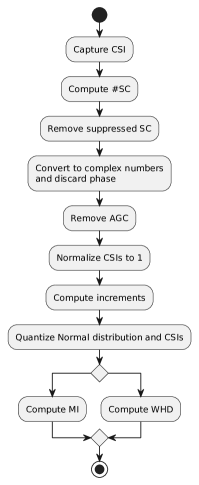
Figure 9.1: Overview of the workflow followed during CSI processing.

Chapter 3 provides a summary of the results produced in the previous work, to improve contextualization of this analysis. The current version of the code maintains backwards compatibility with the processing carried out throughout the BSc Thesis. To support this statement, we reproduce the results showcased in Chapter 3 on the new dataset.

Fig. 9.2 displays the evolution in time of the amplitude of CSI collected on a randomly chosen sub-carrier in two different scenarios. Each plot represents two distinct yet visibly superimposable graphs: in red, referencing the left $y$-axis, the normalized amplitude is displayed, whereas in blue, referencing the right $y$-axis, the quantized version is plotted. Note that the line widths used to represent the two processes have been set to different values to allow distinction of the two series that are otherwise almost exactly superimposed within each of the two scenarios. By observing these figures, we come to the conclusion that CSI amplitude before and after quantization remains structurally unaltered, regardless of the scenario the traces were collected in. As one can expect, the CSI representing a more dynamic scenario (Fig. 9.2(b)) display higher variability in their evolution in time, which highlights how the amplitude indeed reflects the structure of the environment. It must be noted that the removal of the effects of the AGC positively contributes to enhancing the ‘true’ behavior of the CSI, mitigating the fluctuations that their amplitudes undergo and that were more evident in the results commented in [21].

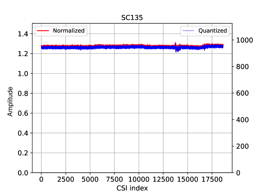
(a) CSI collected on a 20 MHz channel using 802.11ax in an empty room.

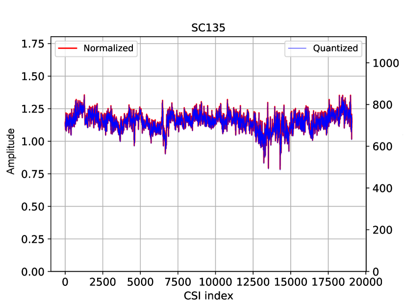
(b) CSI collected on a 20 MHz channel using 802.11ax in a room with four people in it.

Figure 9.2: Example of amplitude evolution in time on sub-carrier 135 in the Empty and Fully Dynamic Scenarios.

To provide a complete evaluation of the available captures, the code developed for [21] was also tested against the AntiSense dataset; an example of the results is showcased in Fig. 9.3.

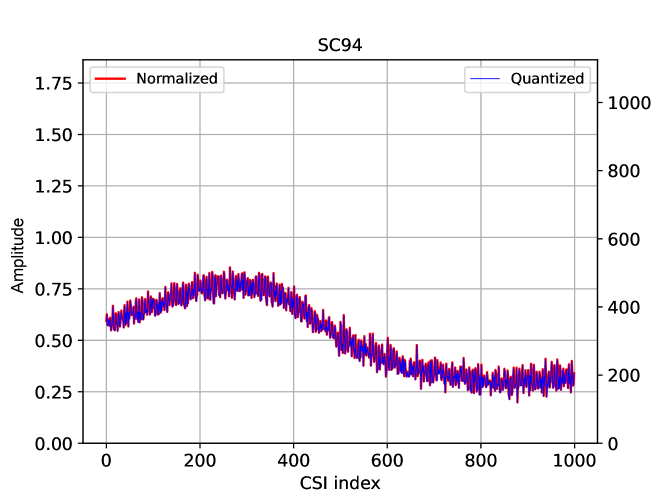
Figure 9.3: Example of amplitude evolution in time on sub-carrier 94. CSI belong to the AntiSense dataset.

Fig. 9.4 displays the distribution of the amplitude increments measured on sub-carrier 135: it can be observed that the histogram resembles a Gaussian distribution, which is coherent with the model proposed in [21].

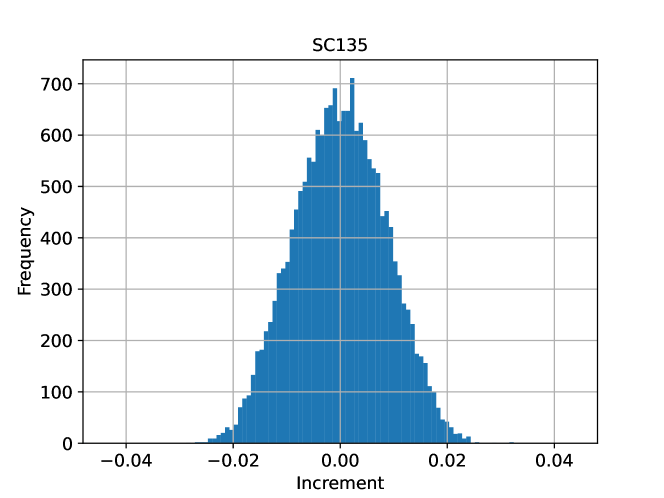
Figure 9.4: Example of increments distribution on sub-carrier 135. CSI were collected on a 20 MHz channel using 802.11ax in an empty room.

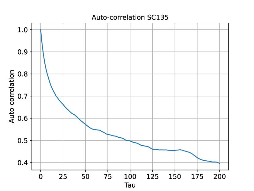
(a) Amplitudes auto-correlation.

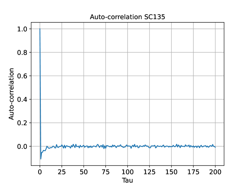
(b) Increments auto-correlation.

Figure 9.5: Examples of amplitudes and increments auto-correlation on sub-carrier 135. CSI collected on a 20 MHz channel using 802.11ax in a room with four people.

Finally, by examining the results of the auto-correlation function computed on the amplitudes (Fig. 9.5(a)), we observe that the process indeed has memory. However, when looking at the auto-correlation of the increments (Fig. 9.5(b)), we find that the function returns noise-like values, which are consistent with the results expected from a Markovian process. Whether such mathematical description could accurately represent the behavior of the increments will be the subject to future further analysis.

10     Results of the Normalization and Quantization Processes

Following the theoretical considerations carried out in Sect. 6.2, we provide a sketch of the implementation of the quantization of $\mathcal{N}(\sigma)$ to obtain $\mathcal{N^{\prime}}(\sigma)$.

The pseudo-code for the quantization process is briefly displayed in the following snippet.

⬇

1 csi = csi - min(csi)

2 csi = csi / max(csi) # CSI ranges from 0 to 1

3 a = 0

4 b = 2 ** (2 * q_amp) - 1

5 csi_quant = round(csi * (b - a) + a) # quantize CSI

6

7 incr = csi.diff() # computes increments using normalized CSI

8 mu, sigma = norm.fit(incr)

9 dstar = 3 * sigma

10 sample = numpy.random.normal(loc=mu, scale=sigma, size=incr.size)

11 sample = filterTails(sample, dstar) # fix boundary conditions

12 # apply the same logic used to quantize amplitudes on increments

13 incr_quant = int(round((sample - min(sample)) / (max(sample) - min(sample)) * (2 ** q_inc - 2) - (2 ** (q_inc - 1) - 1)))

Listing 3: Pseudo-code of the algorithm used to normalize and quantize CSI and increments.

By running this code on the collected data, we create a quantized version of the Normal distribution that is used to approximate the empirical distribution of the increments. This is evident in the presented pseudo-code, as the values of the sample array are randomly selected from a Normal distribution with the same mean and standard deviation as the distribution of the increments. Should the approximation prove ineffective in correctly representing the empirical increments, the overall logic of the code would remain unaltered and all computations would be carried out on the original incr array instead of sample. As stated at the end of Sect. 6.2, we will assume that the Gaussian distribution correctly approximates the increments distribution.

To choose a suitable $q_{\text{\tiny inc}}$ value to quantize the increments and to compute the correct $q_{\text{\tiny amp}}$, values $q_{\text{\tiny inc}}=3,4,5$ have been selected for evaluation. To support the final choice of $q_{\text{\tiny inc}}=4$, we present three histograms comparing the increments obtained from the collected data and an equally large sample of values randomly extracted from the Gaussian distribution, as described in LABEL:lst:normquant. The three plots displayed in Fig. 10.1, 3, 10.2, 3 and 10.3 compare increments and sampled values after quantization over 3, 4, and 5 bits respectively. All three histograms have been normalized with respect to the integral of the distribution and use a logarithmic scale on the $y$-axis to simplify data comparison.

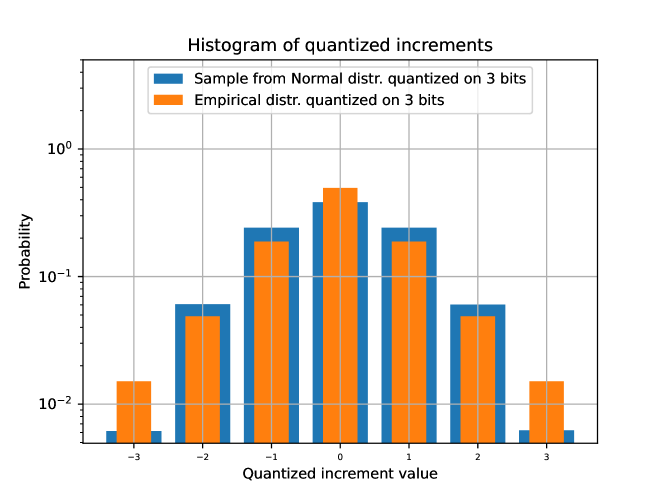
Figure 10.1: Distribution of increments VS sample from Gaussian distribution after quantization over 3 bits. Increments are computed on an experiment performed in the Empty Scenario at 20 MHz.

It is easily observable that the measured increments follow a slightly more peaked trend, with the central and the outermost values (i.e. the tails of the quantized distribution) appearing more often than they do in the sampled version of the increments. In contrast, the intermediate values appear less frequently than in the sampled increments.

Choosing 3 bits to quantize the Gaussian distribution is limiting in terms of information that can be represented. The quantization over 4 bits, even though the resulting empirical distribution has a higher probability of the external intervals compared to the values sampled from the Gaussian distribution, results in a sufficiently informative representation of the increments. Moreover, the tails of the Normal distribution are correctly quantized and do not alter the distribution itself. We will use the Gaussian distribution with 4-bit quantization to approximate the increments, as it allows a sufficiently informative representation of the $\delta_{\mathbf{C}}$ values, without misrepresenting the process due to the use of too many quantization bits.

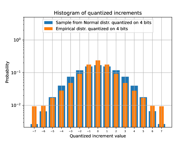
Figure 10.2: Distribution of increments VS sample from Gaussian distribution after quantization over 4 bits. Increments are computed on an experiment performed in the Empty Scenario at 20 MHz.

Contrarily, quantization over 5 bits using $3\cdot\sigma$ to fix boundary conditions results in evident excessive accumulation of the tails of both the Normal and empirical distribution on the boundary quantization intervals; this excludes the possibility of using 5 bits to quantize the Gaussian distribution, as the behavior of its tails is altered.

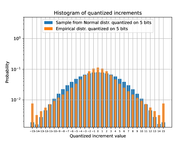
Figure 10.3: Distribution of increments VS sample from Gaussian distribution after quantization over 5 bits. Increments are computed on an experiment performed in the Empty Scenario at 20 MHz.

To further support the choice of $q_{\text{\tiny inc}}=4$, we provide an example of the distribution of the quantized increments of CSI belonging to the AntiSense dataset in Fig. 10.4. In this case, the increments behave almost exactly like the Gaussian distribution, without facing any distortion of the values of the boundary intervals.

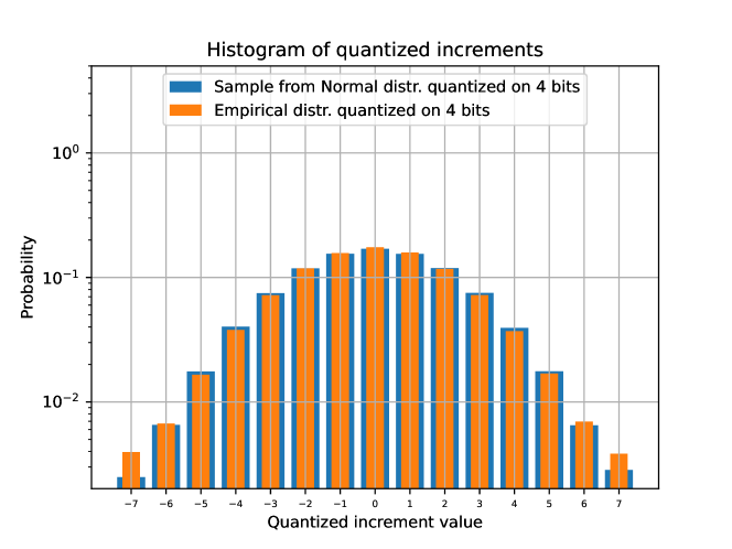
Figure 10.4: Distribution of increments VS sample from Gaussian distribution after quantization over 4 bits. Increments are computed on an experiment belonging to the AntiSense dataset.

Regardless of the number of quantization bits and the technology used to capture the CSI, the original distribution of the increments is symmetric around zero, as can also be seen in Fig. 10.5, 3 and 10.6 where the results of the quantization over 4 bits of the increments computed on traces collected at 40 and 80 MHz are displayed. This consideration remains valid even in those cases where the empirical distribution no longer resembles the Gaussian curve.

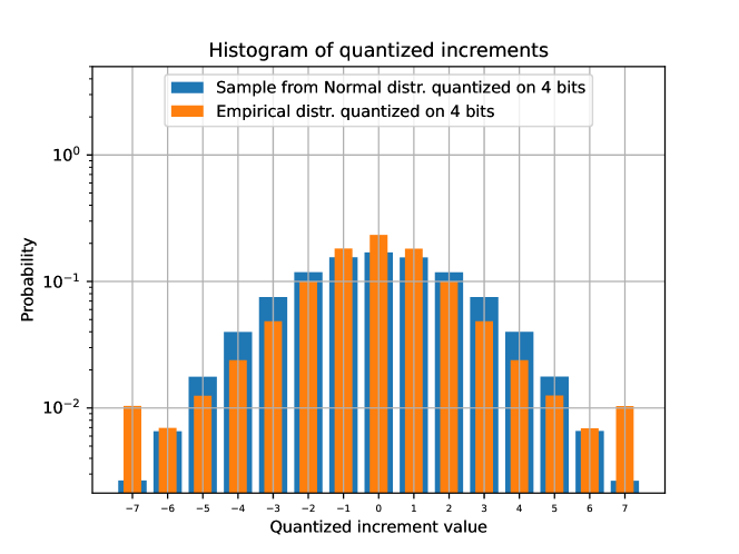
Figure 10.5: Distribution of increments VS sample from Gaussian distribution after quantization over 4 bits. Increments are computed on an experiment performed in the Empty Scenario at 40 MHz.

Figure 10.6: Distribution of increments VS sample from Gaussian distribution after quantization over 4 bits. Increments are computed on an experiment performed in the Empty Scenario at 80 MHz.

Fig. 10.7, 3, 10.8, 3 and 10.9 offer a straightforward comparison between $A_{\mathbf{C}}$ values before and after undergoing quantization. The trends followed by the two processes can be superimposed with an irrelevant mismatch, as highlighted in the third plot of each figure. The third plot is obtained by displaying the difference between normalized $A_{\mathbf{C}}(k,n)$ and the value computed after reversing the quantization process and re-normalizing the resulting values. Regardless of the bandwidth the collection was obtained on, $q_{\text{\tiny amp}}=10$ has been chosen as a function of $q_{\text{\tiny inc}}$, as per Eq. 6.16: this choice should provide a semantically equal representation of the amplitudes across scenarios and experiments, facilitating comparison of the results obtained through different technologies and setups.

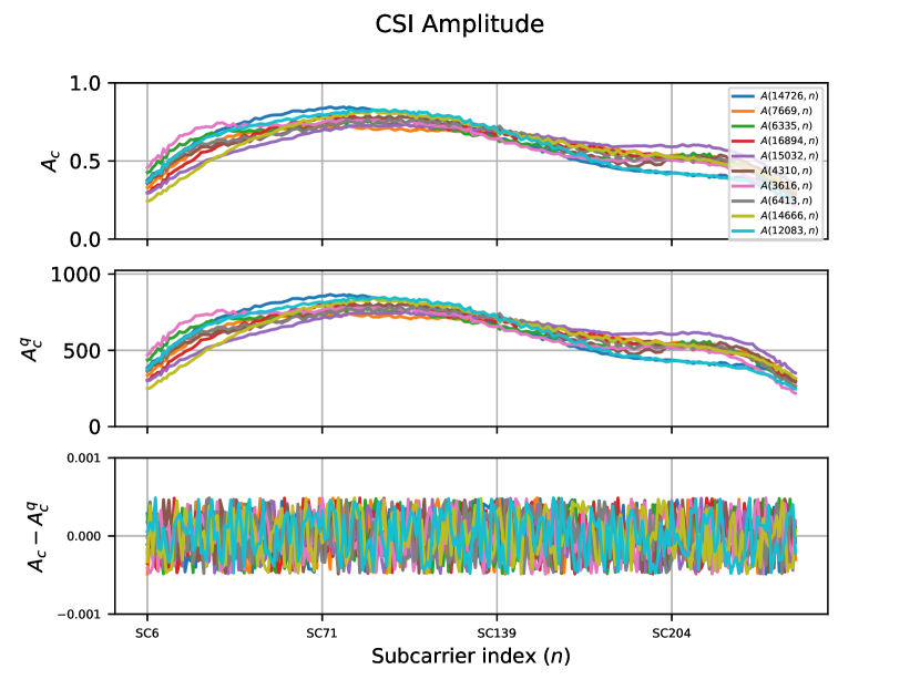
Figure 10.7: Comparison of the structure of $A_{\mathbf{C}}$ before and after quantization. The third plot shows the difference between the original normalized $A_{\mathbf{C}}$ and that obtained after reversing the quantization process and normalizing the result between $0$ and $1$. The represented CSI are randomly selected from an experiment performed at 20 MHz in the Fully Dynamic Scenario, with 4 people in the room.

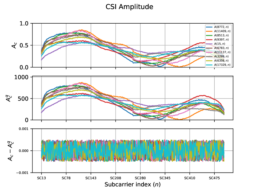
Figure 10.8: Comparison of the structure of $A_{\mathbf{C}}$ before and after quantization. The third plot shows the difference between the original normalized $A_{\mathbf{C}}$ and that obtained after reversing the quantization process and normalizing the result between $0$ and $1$. The represented CSI are randomly selected from an experiment performed at 40 MHz in the Fully Dynamic Scenario, with 5 people in the room.

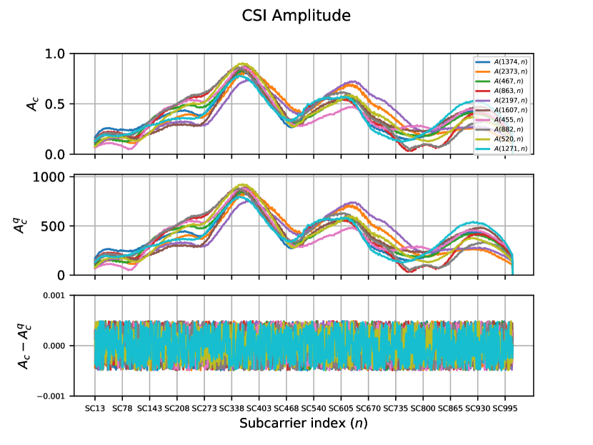
Figure 10.9: Comparison of the structure of $A_{\mathbf{C}}$ before and after quantization. The third plot shows the difference between the original normalized $A_{\mathbf{C}}$ and that obtained after reversing the quantization process and normalizing the result between $0$ and $1$. The represented CSI are randomly selected from an experiment performed at 80 MHz in the Fully Dynamic Scenario, with 5 people in the room.

11     Results of the Analysis of the Weighted Hamming Distance

In Chapter 8, the following different characterizations of the WHD have been introduced:

• Internal: $\text{WHD}(A^{\star}_{\mathbf{C}},A_{\mathbf{C}}(k,\cdot))$ with $A^{\star}_{\mathbf{C}}$ belonging to the same experiment as all $A_{\mathbf{C}}$;

• External: $\text{WHD}(A^{\star}_{\mathbf{C}},A_{\mathbf{C}}(k,\cdot))$ with $A^{\star}_{\mathbf{C}}$ belonging to the same scenario as all $A_{\mathbf{C}}$ but to a distinct experiment;

• Cross-setup: $\text{WHD}(A^{\star}_{\mathbf{C}},A_{\mathbf{C}}(k,\cdot))$ with $A^{\star}_{\mathbf{C}}$ belonging to a different scenario than all $A_{\mathbf{C}}$.

Considering that a 10-minute-long experiment consists of nearly twenty thousand CSI, albeit feasible, computing all distances between each and every CSI and $A^{\star}_{\mathbf{C}}$ would make the discussion of the results ineffective and impossible to compact into a limited yet meaningful amount of data. Therefore, the discussion will initially revolve around the average distances between $A^{\star}_{\mathbf{C}}$ and all $A_{\mathbf{C}}$ of an experiment. The computation of the average WHD will be performed as follows:

$$\overline{\text{WHD}(A^{\star}_{\mathbf{C}},A_{\mathbf{C}})}=\frac{1}{M_{\mathbf{C}}}\sum_{k=1}^{M_{\mathbf{C}}}\text{WHD}(A^{\star}_{\mathbf{C}},A_{\mathbf{C}}(k,\cdot))$$ (11.1)

where $\overline{\text{WHD}(A^{\star}_{\mathbf{C}},A_{\mathbf{C}})}$ employs the symbol $A_{\mathbf{C}}$ to indicate the whole considered experiment through its generic CSI. The classification of the average WHD as internal, external or cross-setup remains the same as that described at the beginning of this chapter.

Together with the average WHD, the standard deviation of the WHD is also computed, to provide a numerical evaluation of the dispersion of the distance values.

Initially, we compute the internal and external $\overline{\text{WHD}}$ under the assumption that the average distance between an experiment and its mean CSI $A^{\star}_{\mathbf{C}}$ should be slightly lower than the external distance of an experiment. Such a difference may not be extremely noticeable (i.e. they may not differ by orders of magnitude) as the compared experiments belong to the same scenario. Data collected in the same scenario is expected to display similar behavior, especially in static environments: the Empty and Static Scenarios, given the minor modifications that the propagation environments undergoes by nature, should produce CSI that are — to some extent — similar to each other.

Since the average distances are computed as floating point values that do not have a reference scale, comparison of the results obtained across different scenarios is ineffective.

To correctly compare the measurements, we normalize the distances dividing each value by the maximum achievable distance. According to the quantization process that each CSI undergoes, the minimum and maximum values that they can take on each sub-carrier are $0$ and $2^{q_{\text{\tiny amp}}}-1$ respectively. Therefore, the minimum distance between two CSI is obviously zero — in case the CSI take the same value on all sub-carriers —, whereas the maximum distance is reached when one CSI is ‘null’ (i.e. zero on all sub-carriers) and the other is equal to $2^{q_{\text{\tiny amp}}}-1$ on all sub-carriers. Hence,

$$0\leq\frac{\overline{\text{WHD}(A^{\star}_{\mathbf{C}},A_{\mathbf{C}})}}{N_{\text{\tiny SC}}\cdot(2^{q_{\text{\tiny amp}}}-1)}\leq 1$$ (11.2)

Using this normalization of $\overline{\text{WHD}(A^{\star}_{\mathbf{C}},A_{\mathbf{C}})}$, the values obtained from different experiments across distinct setups become comparable, as they reference a scale going from 0 to 1. From this point on, $\overline{\text{WHD}(A^{\star}_{\mathbf{C}},A_{\mathbf{C}})}$ will be used to refer to the normalized average WHD, to avoid overloading the notation.

11.1   Results on the Collected Dataset

To answer the question of whether it is easily understandable if a given CSI belongs to a specific experimental setup, Tab. 11.1 presents the normalized average WHD obtained from computing the internal, external and cross-distance between $A^{\star}_{\mathbf{C}}$ and the CSI collected at 20 MHz in the Empty, Static, and Fully Dynamic Scenarios. Values highlighted in yellow represent the internal and external WHD for the Empty, Static and Fully Dynamic Scenarios. Specifically, on the diagonal of the matrix, the values of the internal distances of the experiments are displayed. Values highlighted in green, orange, and blue represent the ‘cross-setup’ distances between each couple of scenarios.

	E0	E1	E2	E3	S0	S1	S2	S3	FD0	FD1	FD2	FD3
$A^{\star}_{\mathbf{C}}$ E0	0.008	0.021	0.021	0.016	0.083	0.069	0.073	0.086	0.145	0.217	0.191	0.108
$A^{\star}_{\mathbf{C}}$ E1	0.021	0.007	0.007	0.012	0.102	0.089	0.091	0.105	0.163	0.231	0.204	0.125
$A^{\star}_{\mathbf{C}}$ E2	0.021	0.007	0.006	0.012	0.102	0.089	0.091	0.105	0.163	0.231	0.204	0.125
$A^{\star}_{\mathbf{C}}$ E3	0.017	0.012	0.012	0.006	0.095	0.082	0.086	0.098	0.153	0.220	0.193	0.115
$A^{\star}_{\mathbf{C}}$ S0	0.081	0.101	0.101	0.094	0.018	0.025	0.032	0.020	0.085	0.155	0.136	0.059
$A^{\star}_{\mathbf{C}}$ S1	0.067	0.087	0.087	0.080	0.025	0.017	0.030	0.029	0.093	0.168	0.147	0.065
$A^{\star}_{\mathbf{C}}$ S2	0.070	0.089	0.088	0.083	0.030	0.026	0.022	0.028	0.102	0.179	0.156	0.072
$A^{\star}_{\mathbf{C}}$ S3	0.084	0.104	0.103	0.097	0.020	0.029	0.030	0.019	0.087	0.159	0.139	0.061
$A^{\star}_{\mathbf{C}}$ FD0	0.142	0.159	0.161	0.150	0.079	0.087	0.097	0.081	0.041	0.108	0.090	0.050
$A^{\star}_{\mathbf{C}}$ FD1	0.212	0.226	0.227	0.216	0.149	0.163	0.174	0.153	0.104	0.049	0.062	0.115
$A^{\star}_{\mathbf{C}}$ FD2	0.187	0.201	0.201	0.190	0.128	0.140	0.151	0.132	0.087	0.063	0.047	0.092
$A^{\star}_{\mathbf{C}}$ FD3	0.106	0.123	0.123	0.113	0.056	0.062	0.070	0.057	0.057	0.122	0.097	0.030

Table 11.1: Normalized average WHD between each experiment performed in the Empty, Static, and Fully Dynamic Scenarios and the reference average CSI computed on the same experiments. Data collected on a 20 MHz channel using 802.11ax. The FD Scenario consisted of four people in the room.

It is evident that the internal WHD always takes the lowest value compared to all other distances — i.e., the lowest values of Tab. 11.1 are on the diagonal of the matrix. Similarly, the highest values of WHD can be found in the blue and orange sub-matrices: this is representative of the fact that the Fully Dynamic Scenario is a more changing environment, which results in more varying CSI traces. Such variability of the environment is reflected in higher distance values.

These considerations can be extended to data collected on the 40 and 80 MHz bandwidths, as can be seen in Tab. 11.2, 3 and 11.3. The color coding of these two tables remains the same as that of Tab. 11.1. Once again, the lowest values can be found on the diagonals of the matrices, corresponding to the internal WHD. Contrarily, the largest differences can be found in the orange sections of the tables, as they contain the distances between the Fully Dynamic and the Empty Scenario: the great variability of the Fully Dynamic Scenario — where multiple people are present in the room and possibly moving around — is compared to the extremely static nature of the Empty Scenario, originating the highest WHD values. This corroborates the assumption that both the presence and the movements of people within an environment significantly affect the behavior of the signal traveling from the transmitter to the receiver.

		EMPTY			STATIC	FULLY DYNAMIC
	# PPL	0	0	0	1	2	3	4	4	5	5
	0	0.004	0.247	0.244	0.232	0.164	0.135	0.169	0.157	0.146	0.169
	0	0.246	0.007	0.008	0.344	0.292	0.184	0.119	0.131	0.175	0.210
EMPTY $A^{\star}_{\mathbf{C}}$	0	0.243	0.008	0.005	0.341	0.289	0.182	0.117	0.129	0.173	0.208
STATIC $A^{\star}_{\mathbf{C}}$	1	0.230	0.344	0.341	0.031	0.182	0.264	0.267	0.259	0.258	0.245
	2	0.150	0.278	0.275	0.168	0.060	0.223	0.201	0.178	0.210	0.182
	3	0.127	0.180	0.179	0.263	0.233	0.044	0.130	0.162	0.096	0.166
	4	0.154	0.099	0.097	0.257	0.211	0.119	0.074	0.094	0.109	0.154
	4	0.134	0.113	0.110	0.245	0.189	0.149	0.087	0.080	0.128	0.154
	5	0.132	0.162	0.160	0.248	0.219	0.082	0.107	0.132	0.067	0.129
FULLY DYNAMIC $A^{\star}_{\mathbf{C}}$	5	0.117	0.183	0.180	0.213	0.176	0.129	0.119	0.124	0.094	0.116

Table 11.2: Normalized average WHD between each experiment performed in the Empty, Static, and Fully Dynamic Scenarios and the reference average CSI computed on the same experiments. Data collected on a 40 MHz channel using 802.11ax.

		EMPTY	STATIC	FULLY DYNAMIC
	# PPL	0	1	2	2	3	4	5
EMPTY $A^{\star}_{\mathbf{C}}$	0	0.005	0.075	0.181	0.163	0.231	0.232	0.221
STATIC $A^{\star}_{\mathbf{C}}$	1	0.072	0.027	0.143	0.128	0.208	0.206	0.188
	2	0.176	0.137	0.047	0.082	0.149	0.142	0.152
	2	0.156	0.122	0.080	0.045	0.160	0.154	0.139
	3	0.228	0.207	0.152	0.161	0.034	0.085	0.111
	4	0.224	0.200	0.139	0.149	0.074	0.055	0.114
FULLY DYNAMIC $A^{\star}_{\mathbf{C}}$	5	0.210	0.176	0.147	0.133	0.101	0.112	0.063

Table 11.3: Normalized average WHD between each experiment performed in the Empty, Static, and Fully Dynamic Scenarios and the reference average CSI computed on the same experiments. Data collected on an 80 MHz channel using 802.11ax.

It is important to highlight that, since the maximum distance between two CSI is an edge case that is extremely unlikely to happen, if not impossible to reach at all, values of the WHD around $0.2$ can be considered large, as they identify substantially different environments. This is supported by the fact that the distance between each experiment and its own $A^{\star}_{\mathbf{C}}$ is in the order of $10^{-2}$ and lower, which means that most collections of CSI are extremely close to their representative CSI $A^{\star}_{\mathbf{C}}$. It is important to note that the Fully Dynamic Scenario intrinsically has such higher variability compared to other experimental setups that the computation of the distances on this scenario may be affected by the significant variations of the amplitudes in the captures.

Tab. 11.1, 3, 11.2, 3 and 11.3 all display the interesting feature of being almost symmetrical. Semantically, symmetry means that comparing an experiment $A$ with the average CSI of experiment $B$ produces the same result that can be obtained by comparing $B$ with the average CSI of $A$. In this case, comparing experiments consists in computing the normalized $\overline{\text{WHD}}$ between them, as per Eq. 11.1, 3 and 11.2. Especially in the Empty Scenario, the modifications that the environment undergoes are microscopic, therefore the symmetry of the matrix is more accentuated. Contrarily, more dynamic scenarios are subject to more impactful and macroscopic alterations, which implies the possibility of less symmetric distances.

Exact symmetry of the external or cross-setup $\overline{\text{WHD}}$ between experiments is difficult to obtain: the $\overline{\text{WHD}}$ is computed as the average distance between each CSI of an experiment $A$ and the average CSI of another experiment $B$. Since the average CSI is a summarized visualization of a whole experiment, its use implies that some information about the experiment is discarded or lost, decreasing the accuracy of the representation. Nonetheless, comparing all experiments CSI by CSI would result in an unmanageable amount of distances, therefore it is necessary to merge such information into a single significant number for each couple of experiments. Computing, once again, an average implies losing some additional information, which can result in minimal — or more significant, depending on the case — asymmetries of the $\overline{\text{WHD}}$ values. The average WHD is deemed an initial effective approach to the computation of the ‘distance’ between CSI captures and is used as a preliminary metric to evaluate the behavior of the collected data. Should a more effective metric be identified, the $\overline{\text{WHD}}$ could still be used as an approximated indicator of the similarity between captures, while for a more detailed description of the experiments the new metric would be used.

To provide a more compact visualization of the average internal distances depending on the experiment, we focus the categorization of the collections of CSI on the number of people that were in the room when the data was captured. This way, we can summarize the values of the internal distance in distributions of the WHD, which allow us to avoid the computation of the average WHD. Such an approach simplifies comparison between the different experimental setups, allowing to infer how the CSI are modified according to the variability of the environment: before looking at the resulting distributions, we can assume that the Empty and Static Scenarios will undergo fewer modifications than the Fully Dynamic one, as the latter also encompasses movements of people in the room, whereas the former are only affected by the furniture and appliances and, possibly, the presence of a person sitting almost still. Therefore, the distributions of distances relative to an Empty or Static Scenario can be expected to be much less spread out than those describing a Fully Dynamic Scenario with four or five people moving around the room. These considerations are supported by figure Fig. 11.1.

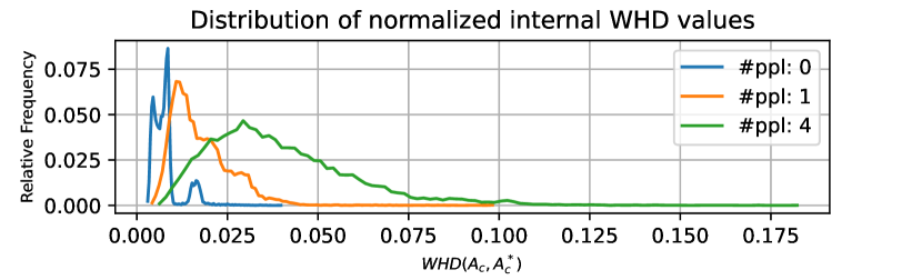
(a) 20 MHz bandwidth.

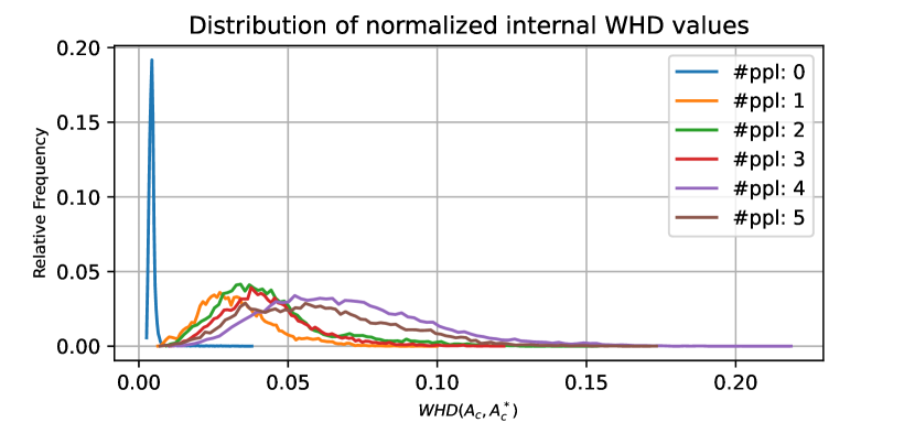
(b) 40 MHz bandwidth.

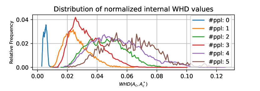
(c) 80 MHz bandwidth.

Figure 11.1: Distribution of the normalized internal WHD across different experiments, each characterized by a distinct number of people in the environment.

In Fig. 11.1(a) we can observe that the distribution of the internal WHD derived from data collected in an empty room is significantly more peaked compared to the distributions relative to the Static and Fully Dynamic Scenarios. By juxtaposing the three distributions, we can notice that the increasing number of people altering the structure of the experimental setup with their movements impacts the spread-out of the distributions.

Fig. 11.1(b) highlights how easily distinguishable the Empty Scenario is compared to any other scenario. This means that the Empty Scenario is extremely self-similar, with internal distances being the closest to 0 across all scenarios. Looking at the other distributions, they maintain the expected behavior of an increasing standard deviation as the number of people in the room grows, albeit they are often overlapped.

The same considerations can be made about the distributions in Fig. 11.1(c), with the Empty Scenario clearly distinct from all others and the remaining experiments showing an increasingly higher dispersion of the distances. It can be noted that, since the 5-people Fully Dynamic Scenario consists of one-minute-long experiments — compared to the 10 minutes of the other captures —, the behavior of the corresponding distribution is slightly more fluctuating than the other ones due to the fewer available CSI to compute the WHD on.

It is necessary to state that analyzing the dispersion of the distances is insufficient to determine the number of people within the room: while the Empty Scenario is easily distinguishable from the others, telling Dynamic Scenarios apart based on the WHD distributions alone is a tough task, due to the distributions being significantly overlapped. A more in-depth and sophisticated analysis is required to determine a tool or metric to perform this task.

Nevertheless, an intuitive representation of the differences between captures collected with a varying number of people in the room is provided by Fig. 11.2, 3, 11.3, 3, 11.4, 3 and 11.5. Each figure represents the comparison between two experiments performed on either the 40 or the 80 MHz bandwidth. The first two plots of each figure represent the evolution in time of the quantized CSI amplitude for the selected experiments: the $y$-axis corresponds to the sub-carriers (excluding those suppressed in transmission) and the $x$-axis represents the CSI index within the experiments. The third plot depicts the difference between the first two (specifically, the first minus the second). The color bar indicates that lower amplitude — or difference — values correspond to the color blue and that higher ones are red, with $0$ being white.

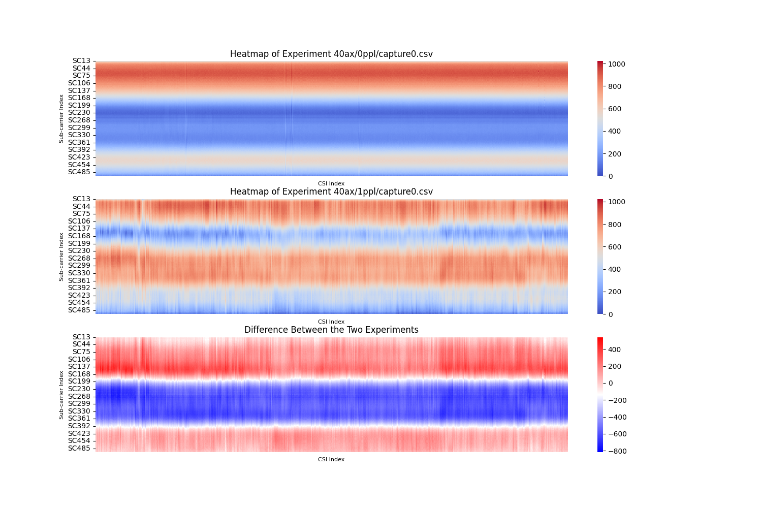
Figure 11.2: Difference in quantized CSI amplitude values between an experiment performed in the Empty Scenario and one in the Static Scenario. The third heatmap depicts their difference. Data collected on a 40 MHz bandwidth channel using 802.11ax.

These figures allow us to easily identify the overall structure of an experiment: for instance, in Fig. 11.2 we can observe that the first heatmap, describing an experiment performed in the Empty Scenario, maintains a static behavior over time on each sub-carrier, with higher amplitude values in the first 150 sub-carriers and lower values in the central band. Similarly, the amplitude trend of the central heatmap — relative to an experiment performed in the Static Scenario — keeps a stationary behavior with lower absolute values. As can be seen in the third plot, the difference between the two scenarios is very distinct, as the three main ‘bands’ that can be identified in the heatmap take on values that are far from $0$. This simple consideration allows for the hypothesis that the two scenarios will be easily distinguishable from one another, as their difference is hardly ever close to zero.

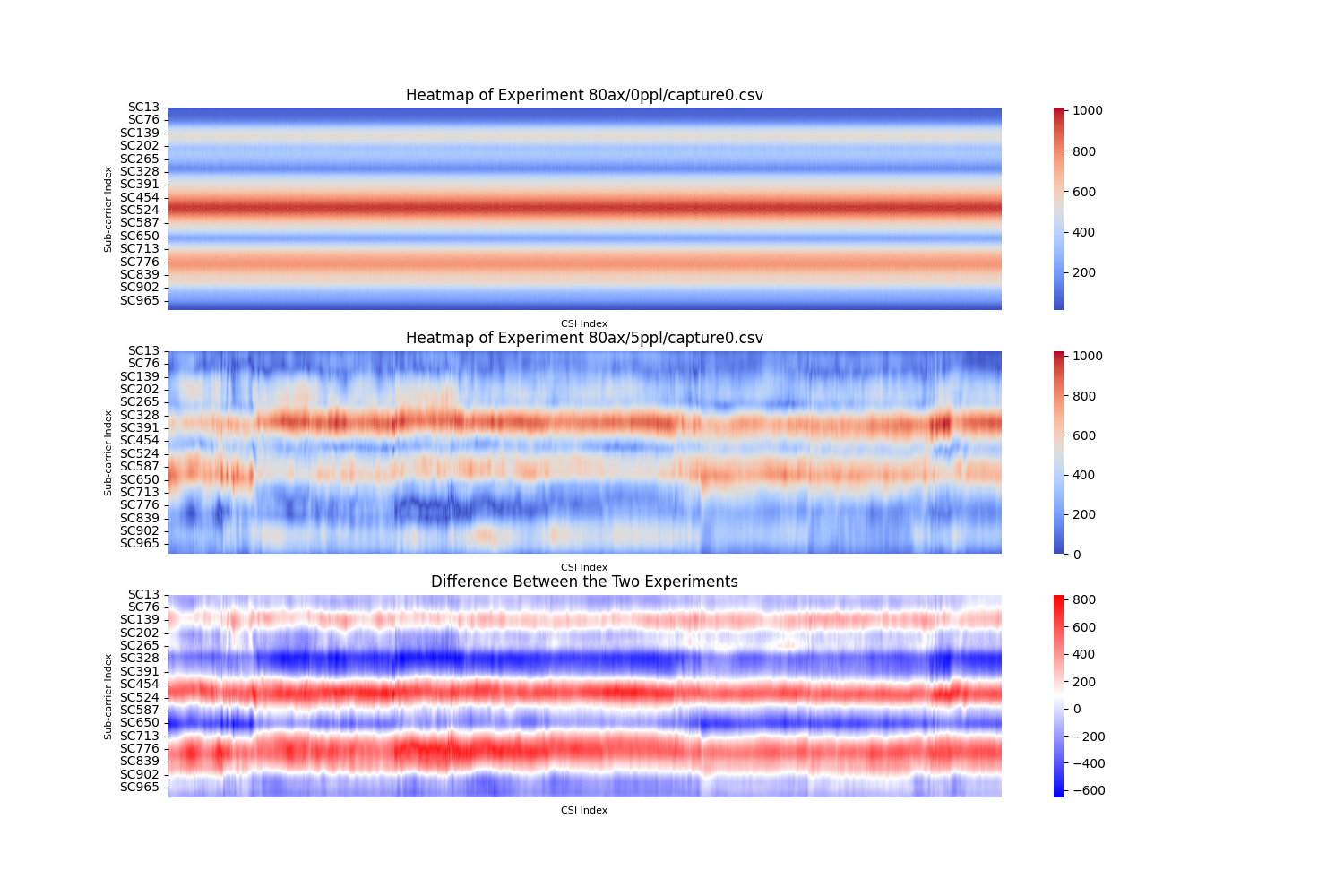
Figure 11.3: Difference in quantized CSI amplitude values between an experiment performed in the Empty Scenario and one in the Fully Dynamic Scenario with 5 people in the room. The third heatmap depicts their difference. Data collected on an 80 MHz bandwidth channel using 802.11ax.

Similar considerations can be made on the CSI represented in Fig. 11.3: the Empty Scenario is characterized by an extremely static behavior in time, whereas the Fully Dynamic Scenario with five people in the room has more variable amplitudes. In this second experimental setup, by looking at each sub-carrier by itself, we can observe that they all undergo modifications in time, necessarily due to the alterations of the environment due to the presence of multiple people. This implies that the higher variability of the Fully Dynamic Scenario makes it easily distinguishable from the Empty one.

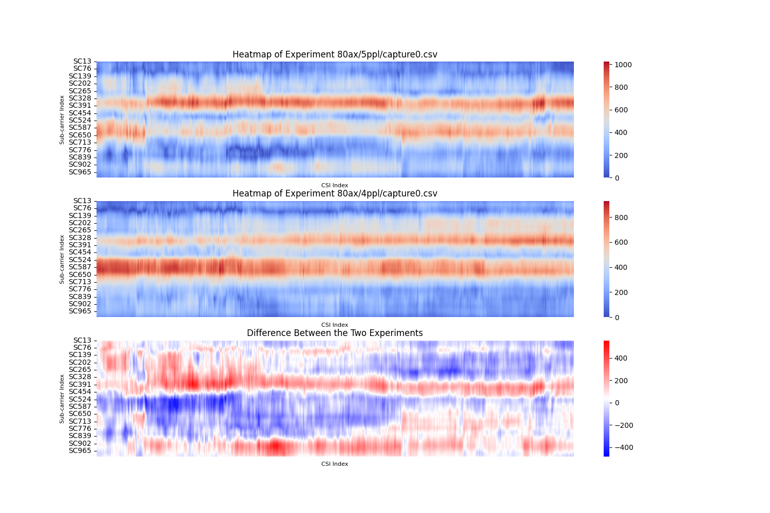
Figure 11.4: Difference in quantized CSI amplitude values between two experiments performed in the fully Dynamic Scenario with 5 and 4 people in the room. The third heatmap depicts their difference. Data collected on an 80 MHz bandwidth channel using 802.11ax.

Fig. 11.4 indicates the opposite situation: the two analyzed experiments were both performed in the Fully Dynamic Scenario with 5 and 4 people in the room respectively. As can be noticed in the third heatmap, the difference between the two collections is more limited compared to the previous examples, especially in the second half of the experiment. It is also less definite in its structure, as the colored bands are much more variable in height and color intensity, indicating that distinguishing between the two scenarios may be less straightforward.

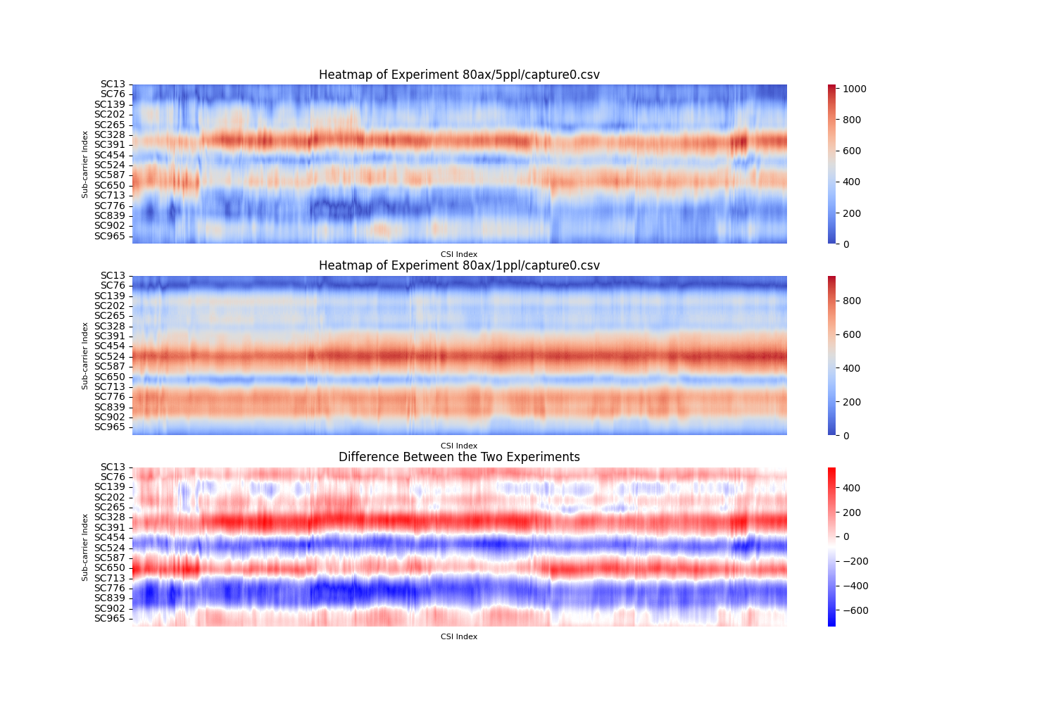
Figure 11.5: Difference in quantized CSI amplitude values between an experiment performed in the Fully Dynamic Scenario with 5 people in the room and one in the Static Scenario. The third heatmap depicts their difference. Data collected on an 80 MHz bandwidth channel using 802.11ax.

Contrarily, comparing the Fully Dynamic Scenario (5 people) with the Static one (see Fig. 11.5) results in more marked differences that set the two environments apart.

Since these results and figures provide a more qualitative insight into the differences between two experiments, a metric to quantify such distance needs to be introduced. The goal would be to produce a distribution of CSI around the average CSI of each experiment; the main difficulty in achieving this characterization of the captures consists in finding a one-dimensional representation of a CSI, accounting for the amplitude values on all sub-carriers simultaneously.

11.2   Results on the AntiSense dataset

Considering that the goal of this work is to provide a mathematical background to ML-based positioning and localization algorithms, testing the code written to carry out the current analysis against CSI traces that have already been classified through ML techniques could provide quantitative results that support such classifications.

Similarly to what has been done for the 20, 40, and 80 MHz bandwidth, we provide a summary of the normalized $\overline{\text{WHD}}$ computed on the data within the AntiSense dataset.

The results showcased in Tab. 11.4, 3 and 11.5 highlight that each experiment is significantly self-similar, as the normalized $\overline{\text{WHD}}$ between each capture and its $A^{\star}_{\mathbf{C}}$ is at most in the order of $10^{-2}$. This initial consideration can be observed on the main diagonal of the two matrices.

The green and blue sub-matrices represent the distance between the training and testing partitions of the dataset; their contents allow to highlight the correspondences between the values of the WHD and the performances of the neural network used in [11] to carry out the positioning task. By observing the green matrix in Tab. 11.4, we can see that some values on its diagonal significantly differ from those in the yellow matrix on its left, especially for experiments 3, 5, 6, 7, and 8. This result should correspond to degraded performances of the neural network: the larger the distance between testing and training, the more likely a neural network is to misinterpret the corresponding data, classifying a set of CSI as belonging to the wrong experimental setup. If the positioning results obtained from evaluating the WHD are consistent with those produced by the neural network in [11], the WHD would gain significance and reliability.

		TRAINING								TESTING
	POS	1	2	3	4	5	6	7	8	1	2	3	4	5	6	7	8
	1	006	232	019	033	179	019	054	047	066	256	223	036	047	263	259	232
	2	231	019	242	210	102	243	180	189	167	034	037	201	235	061	052	041
	3	016	242	009	036	189	020	065	055	076	266	233	045	051	274	269	241
	4	033	211	038	006	160	039	040	036	050	236	201	017	047	243	238	210
	5	178	103	189	159	018	183	158	160	144	112	102	153	172	113	112	109
	6	019	243	023	039	018	007	065	057	078	266	235	046	045	273	269	243
	7	054	180	066	039	158	065	009	024	034	205	173	033	062	213	207	182
$A^{\star}_{\mathbf{C}}$ TRAINING	8	047	190	057	035	161	057	023	010	031	216	180	029	061	224	218	187
	1	066	168	077	050	145	077	034	031	007	193	158	042	074	202	196	167
	2	255	036	267	236	113	266	205	216	192	014	048	227	259	049	055	053
	3	223	040	234	201	102	235	173	180	158	048	016	192	227	062	063	041
	4	034	202	045	016	154	046	032	029	042	227	192	009	048	234	229	201
	5	040	233	045	039	170	037	056	057	069	257	224	043	017	264	259	233
	6	263	062	275	243	113	273	213	223	202	049	061	234	265	017	059	075
	7	258	051	270	238	111	269	206	218	196	052	061	229	260	059	021	054
$A^{\star}_{\mathbf{C}}$ TESTING	8	232	042	242	209	109	243	182	187	167	052	039	201	235	075	055	017

Table 11.4: Normalized average WHD computed on the partitions of the AntiSense dataset dedicated to training and testing with the receiver located in position 1 (rx1). The integer values are the first three digits after the comma, rounded to the nearest value. The POS parameter indicates the position of the person standing still within the experimental environment.

By looking at the results of [11], many of these larger WHD values are consistent with misclassifications by the neural network: over 1000 samples, the neural network has a success rate of over 90% (except for ‘rx5’, which will be discussed later) but the classifications relative to ‘rx1’ show higher failure rates for experiments 3, 6, 7, and 8, which is coherent with the content of Tab. 11.4. Unfortunately, the average WHD is too ‘summarizing’ to be used for classification while expecting the same level of precision and detail as a neural network.

The results relative to the set of experiments tagged ‘rx5’ under ‘active attack’ were not analyzed in depth in [11], as the classification performed by the neural network was close to a random guess. Tab. 11.5 contains the $\overline{\text{WHD}}$ values relative to the experiments performed in such setup of the laboratory, where the receiver was placed extremely close to the transmitter; this caused the CSI to be dominated by the transmitted signal itself rather than reflecting the modifications it undergoes after propagating through the environment. Whether we observe the training or testing partition of the dataset, the distances contained in Tab. 11.5 are all similar to each other, regardless of the compared experiments. This behaviour directly impacted the performance of the neural network used in the cited work, as values that are similar across all experiments make it harder to correctly classify a collection of CSI as belonging to a specific experimental setup.

		TRAINING								TESTING
	POS	1	2	3	4	5	6	7	8	1	2	3	4	5	6	7	8
	1	006	012	010	007	013	021	011	018	017	017	010	008	011	010	022	035
	2	012	006	007	011	008	012	010	011	009	008	008	012	008	007	014	025
	3	010	007	005	010	009	013	010	012	010	010	006	010	008	008	015	027
	4	007	011	010	006	012	019	011	016	016	016	010	007	010	010	021	033
	5	013	008	009	012	006	011	011	011	010	009	010	012	007	008	014	023
	6	021	012	013	019	011	006	015	010	008	009	015	019	013	014	011	015
	7	011	009	009	010	011	014	007	014	012	013	010	011	010	010	017	028
$A^{\star}_{\mathbf{C}}$ TRAINING	8	018	011	011	016	011	010	014	007	010	010	013	017	012	013	012	018
	1	017	010	010	016	010	009	013	011	005	008	012	016	011	011	012	019
	2	017	009	010	016	009	009	013	011	008	005	011	016	011	011	011	019
	3	010	008	006	010	011	015	011	013	012	011	006	010	009	008	017	028
	4	008	011	010	007	012	019	011	017	015	016	010	006	011	010	021	033
	5	011	007	008	011	007	013	010	012	011	011	009	011	006	008	016	026
	6	010	008	008	010	009	014	011	013	011	011	008	010	008	006	016	027
	7	022	013	015	020	013	009	017	011	011	010	016	021	015	015	008	016
$A^{\star}_{\mathbf{C}}$ TESTING	8	035	025	026	033	023	015	028	018	019	019	028	033	026	027	016	006

Table 11.5: Normalized average WHD computed on the partitions of the AntiSense dataset dedicated to training and testing with the receiver located in position 5 (rx5). The integer values are the first three digits after the comma, rounded to the nearest value. The POS parameter indicates the position of the person standing still within the experimental environment.

These results confirm the behavior of the neural network, while simultaneously allowing to make preliminary predictions on its ability to succeed in locating a person within the chosen room. Hence, the $\overline{\text{WHD}}$ turns out to be a useful metric that can be exploited to make assumptions on the quality of the performance of neural networks in the positioning task. Nonetheless, it is still too coarse a metric to grasp the subtleties in CSI values that a neural network is capable of identifying, making it hard to position a person within a room based solely on the WHD.

The three tables that have not been explicitly commented in this section can be found in App. B, but the results of the analysis that was carried out on Tab. 11.4, 3 and 11.5 remain consistent if extended to those tables as well.

12     Conclusions and Future Work

This work took off from the findings of the Bachelor’s Degree Thesis and focused on expanding the characterization of a Wi-Fi channel through CSI analysis. Given the complexity of the goal, the study was centered on the amplitude of the CSI, temporarily discarding the phase values.

To favor a step-by-step approach, the work was subdivided into multiple tasks, the first consisting in identifying a representation of CSI amplitudes that can simplify the comparison of the values across different experimental setups. For each CSI, other than normalizing its amplitudes by the integral of the energy to remove the effect of the AGC, the values it takes on each OFDM sub-carrier are normalized between 0 and 1 and then quantized on a finite number of bits. The quantization allows for a more compact representation of the CSI, introducing an upper bound to the amplitudes that was not implicitly present upon CSI extraction. This approach lets us describe the traces on a closed set of finite values that remains unaltered across the different experiments, facilitating simultaneous analysis and comparison of the results relative to different captures, possibly even done with distinct technologies.

Once a unique representation for the CSI had been found, the second task consisted in considering each collection of traces as a source of information about the environment, which meant quantifying the amount of knowledge carried by each CSI. This sub-goal was first approached through the computation of MI, which should provide a measure of the information that can be gathered about ‘environment A’, given a capture performed in ‘environment B’. Computing the MI has proven less straightforward than expected, as each CSI has one in $2^{N_{\text{\tiny SC}}\cdot q_{\text{\tiny amp}}}$ chances of ‘happening’, which of course results in unmanageable values, given that the number of useful sub-carriers is $N_{\text{\tiny SC}}=256,\leavevmode\nobreak\ 512,\leavevmode\nobreak\ 1024$ and the quantization bits are $q_{\text{\tiny amp}}=10$. Nonetheless, this approach would have allowed us to account for the probability of a CSI belonging to a specific experiment, making MI a possibly extremely useful metric for the environment classification task. Therefore, more research is needed to see whether the MI could come in handy if its computation is implemented following an alternative path.

To avoid incurring problems linked to the numerical representation of the information content of CSI, the study was redirected towards the measurement of the WHD between two CSI traces. This metric calculates the number of mismatching bits in the binary representation of two quantized CSI, resulting in the determination of the number of differences between such traces. By switching to the integer representation of the quantized CSI, the weight of the differing bits within the two traces is automatically accounted for, making mismatches in more significant bits more impactful on the resulting distance.

As the WHD can only be computed between single CSI, the comparison of whole experiments was carried out by measuring the WHD between the reference CSI of the first experiment and all CSI of the second one and then averaging them. To ensure symmetry of the distances, the inverse was also computed. Results show that each capture is extremely self-similar (i.e., the average WHD between an experiment and its reference CSI is close to zero), with increasingly larger values as the variability of the experimental setup grows. For instance, as the number of people in the room where the CSI were collected increases, thus causing more changes in the environment, the distance between different experiments grows. As can be imagined, the smallest distances can be found in correspondence to the Empty Scenario (i.e., an empty room), whereas the largest ones can be obtained by comparing it with the Fully Dynamic Scenario with five people in the room.

By only looking at the results relative to the WHD, we do not have enough information to tell environments apart based solely on the dispersion of the average distance from the reference CSI representing an experiment. Specifically, this task can only be carried out for the Empty Scenario, as its variability is minimized and the distances from the reference CSI are less dispersed, but, as the number of people in the room increases, the distribution of the average WHD loses such powerful meaning.

Further research is needed to identify an ulterior metric that allows comparison of the distribution of CSI: such a representation of the dispersion of CSI within each capture would make it possible to find any overlap in the distributions relative to different experiments, enabling the computation of the probability of wrongly classifying an experimental setup. Reaching this goal would provide mathematical and probabilistic support to ML classification algorithms, offering an insight into how they work and reducing their use as ‘black boxes’.

This work paves the road to such extension, having introduced a quantization mechanism to simplify manipulation of CSI amplitudes, providing a method to view them as items within a finite set, which significantly simplifies theoretical reasoning and computations.

Acknowledgments

The work of this thesis has been carried out within the framework of PNRR-funded research projects granted to the Department of Information Engineering at the University of Brescia, PI the supervisor of this thesis. In particular, the topic of CSI analysis lies at the base of these two projects:

• Joint Communication and Sensing: CSI-Based Sensing for Future Wireless Networks (CSI-Future), PRIN 2022 PNRR Prot. P2022FP9W3 (CUP D53D23016040001);

• RESearch and innovation on future Telecommunications systems and networks, to make Italy more smART (RESTART – PE00000001) funded by the European Union (EU) and the Italian Ministry for Universities and Research (MUR), National Recovery and Resilience Plan (NRRP), Spoke 4, Structural Project SUPER, Cascade Call Project “Architettura, PROgetto, ottimizzazione e valutazione di sistemi di percezione collaborativa distribuiti per Smart Driving Spaces” (PROSDS – CUP C89J24000270004).

Appendix A Detailed Classification of Collected Data

The collection of the CSI traces used in this work is obtained through multiple experiments, which are classified according to metadata that is specific to each set of captures.

Each experiment consists of a single capture of CSI performed within a continuous period of time; stopping the traces capture and restarting it after a few minutes have passed without altering any configuration parameter still counts as the end of an experiment and the start of a new one. This leads to the possibility of having multiple experiments with the same configuration, hence the same metadata can be shared among different captures.

The metadata are structured as fields of a json file, containing all information required to classify an experiment. The content of the file is organized as follows:

• Date: day, month, and year where the capture took place. All three sub-fields are integer values;

• Location ID: the unique identifier of the environment where the capture took place. The association of each ID with the corresponding description (e.g. the address or the geographical coordinates of the location) is contained in a separate file, as will be described further on;

• Experiment: a string that describes the type of experiment performed;

• Ad hoc transmission: a boolean field that qualifies the traffic transmitted through the environment as artificially or user-generated;

• usleep: integer value indicating the interval — in microseconds — between each transmitted packet and the following one;

• Average duration: integer value indicating the duration (on average) of an experiment associated with the current metadata. The duration is expressed in seconds;

• Bandwidth: integer value indicating the bandwidth of the channel used to transmit traffic;

• Modulation: string indicating the type of 802.11 modulation used for transmission;

• Number of receivers: integer value indicating the number of receivers involved in the experiment;

• Number of transmitters: integer value indicating the number of transmitters involved in the experiment;

• Number of antennas used at the transmitter (integer);

• Number of antennas used at the receiver (integer);

• People: field used to identify the presence of people in the location where the experiment was performed. It is composed of four sub-fields:

  • Present: boolean field to state if anyone was within the environment where the CSI were captured;

  • Number: integer value indicating the number of people in the location;

  • Moving: boolean field assessing whether the people in the room are walking around or standing still/sitting down. If no one is in the room, this field is set to false;

  • Names: list of the names of the people in the room (if any, empty list otherwise).

• Notes: additional information that is deemed relevant.

To uniquely identify the locations of the experiments, an additional json file is generated, which contains all location IDs and corresponding descriptions.

This description of the classification of the captures corresponds to the latest version employed up to September 2024. Studies after this date may alter the structure of the json files containing the metadata of each experiment or even base the classification on entirely different mechanisms.

All CSI traces collected within this study will be published as open data according to the necessities of the projects listed in the acknowledgements of this work.

Appendix B Normalized Average WHD of the AntiSense Dataset

The tables containing the normalized $\overline{\text{WHD}}$ computed on the AntiSense dataset that were not explicitly commented in Chapter 11 are here displayed. They reference the experiments identified as ‘rx2’, ‘rx3’, and ‘rx4’ according to the position of the receiver, as shown in Fig. 4.2.

		TRAINING								TESTING
	POS	1	2	3	4	5	6	7	8	1	2	3	4	5	6	7	8
	1	009	028	023	017	024	025	028	032	028	029	023	022	020	023	028	036
	2	028	010	024	021	028	022	026	028	036	015	026	025	026	023	024	029
	3	023	025	008	019	021	018	027	020	026	024	015	029	022	020	023	025
	4	018	022	019	009	020	021	024	025	028	021	020	016	018	019	023	030
	5	024	028	021	020	010	020	030	026	023	028	019	026	012	018	028	029
	6	025	021	017	020	019	011	024	023	029	021	019	026	020	015	022	028
	7	027	026	026	023	029	024	012	027	041	024	028	021	030	021	021	033
$A^{\star}_{\mathbf{C}}$ TRAINING	8	032	028	020	025	026	024	027	010	032	029	021	030	028	023	025	017
	1	028	036	026	028	023	030	042	032	009	037	021	035	022	030	033	032
	2	029	015	024	021	028	022	025	029	037	009	026	023	027	022	024	032
	3	023	026	014	019	019	021	029	021	021	026	009	027	018	019	023	023
	4	022	025	029	016	027	027	023	030	035	023	027	009	022	024	028	034
	5	020	026	022	018	012	021	031	028	022	027	018	022	009	019	029	030
	6	024	024	019	019	018	016	022	023	030	022	019	023	019	009	022	028
	7	027	024	022	022	027	023	021	024	032	023	022	027	028	021	011	026
$A^{\star}_{\mathbf{C}}$ TESTING	8	036	029	024	029	028	028	033	017	032	031	023	034	030	028	027	010

Table B.1: Average normalized WHD computed on the partitions of the AntiSense dataset dedicated to training and testing with the receiver located in position 2 (rx2). The integer values are the first three digits after the comma, rounded to the nearest value. The POS parameter indicates the position of the person standing still within the experimental environment.

		TRAINING								TESTING
	POS	1	2	3	4	5	6	7	8	1	2	3	4	5	6	7	8
	1	018	051	065	076	071	057	086	116	036	049	074	226	073	064	070	131
	2	045	027	053	058	078	052	077	118	052	037	063	213	070	063	060	143
	3	064	055	021	072	089	073	086	117	079	062	038	190	083	084	071	139
	4	076	063	073	016	068	064	055	080	072	073	088	203	064	066	053	107
	5	069	080	088	065	021	057	053	077	067	088	112	217	035	050	046	092
	6	056	055	075	062	058	020	057	088	050	066	090	232	048	030	048	113
	7	086	080	087	053	054	058	020	066	082	091	107	206	050	056	033	097
$A^{\star}_{\mathbf{C}}$ TRAINING	8	114	119	116	079	075	085	065	026	111	129	140	215	081	083	076	043
	1	036	057	080	072	068	051	083	113	017	061	090	245	069	051	070	132
	2	050	042	063	073	089	067	092	130	061	017	073	222	082	080	076	156
	3	073	067	040	088	113	091	107	141	089	073	019	179	105	102	091	164
	4	226	213	190	202	217	232	206	215	245	222	179	010	222	228	197	207
	5	072	073	083	062	036	049	050	083	068	082	105	222	019	041	047	106
	6	064	066	085	066	050	031	056	086	051	080	102	228	042	018	049	109
	7	070	064	072	052	047	049	033	078	069	076	091	197	048	048	018	106
$A^{\star}_{\mathbf{C}}$ TESTING	8	131	145	139	107	092	113	096	046	132	156	164	207	106	109	106	020

Table B.2: Average normalized WHD computed on the partitions of the AntiSense dataset dedicated to training and testing with the receiver located in position 3 (rx3). The integer values are the first three digits after the comma, rounded to the nearest value. The POS parameter indicates the position of the person standing still within the experimental environment.

		TRAINING								TESTING
	POS	1	2	3	4	5	6	7	8	1	2	3	4	5	6	7	8
	1	021	052	201	057	225	052	089	169	033	063	038	063	260	047	069	087
	2	053	020	221	061	232	052	085	186	048	033	044	057	275	054	064	083
	3	200	220	011	236	211	213	249	054	226	230	212	242	111	214	229	252
	4	059	061	236	019	260	049	068	201	043	063	046	037	300	050	058	066
	5	224	231	208	259	035	246	254	211	234	240	230	248	196	237	244	253
	6	051	053	213	048	247	020	073	177	043	059	050	047	275	037	058	065
	7	089	085	249	067	255	071	022	213	075	073	079	067	305	068	039	052
$A^{\star}_{\mathbf{C}}$ TRAINING	8	169	187	052	201	217	177	213	016	193	199	180	206	137	180	194	217
	1	035	050	227	043	236	045	076	193	017	059	034	050	282	042	062	071
	2	065	035	231	064	242	061	074	199	059	016	053	063	293	061	058	077
	3	041	046	213	046	231	053	080	180	035	052	016	055	274	050	065	077
	4	063	057	243	035	249	046	067	206	048	061	053	021	300	052	056	060
	5	258	273	105	299	194	274	304	132	281	290	273	299	023	271	284	306
	6	046	053	215	048	239	035	067	180	038	057	046	051	273	023	055	062
	7	068	063	230	055	245	055	038	194	059	055	062	054	285	055	024	054
$A^{\star}_{\mathbf{C}}$ TESTING	8	085	081	252	063	254	062	050	217	068	074	073	059	308	059	054	027

Table B.3: Average normalized WHD computed on the partitions of the AntiSense dataset dedicated to training and testing with the receiver located in position 4 (rx4). The integer values are the first three digits after the comma, rounded to the nearest value. The POS parameter indicates the position of the person standing still within the experimental environment.

Ringraziamenti

References

- [1] Erik Lamers et al. “Securing home Wi-Fi with WPA3 personal” In 2021 IEEE 18th Annual Consumer Communications & Networking Conference (CCNC), 2021, pp. 1–8 IEEE
- [2] WiFi Alliance “WPA3 Specification Version 3.3” Accessed: 2024-08-24, 2024 URL: https://www.wi-fi.org/system/files/WPA3%20Specification%20v3.3.pdf
- [3] Chenwei Cai, Li Deng, Mingyang Zheng and Shufang Li “PILC: Passive Indoor Localization Based on Convolutional Neural Networks” In IEEE Ubiquitous Positioning, Indoor Navigation and Location-Based Services (UPINLBS), 2018, pp. 1–6
- [4] Yan Wang et al. “E-Eyes: Device-Free Location-Oriented Activity Identification Using Fine-Grained WiFi Signatures” In Proc. of the ACM 20th Int. Conf. on Mobile Computing and Networking (MobiCom’14), 2014, pp. 617–628
- [5] Christoph Studer et al. “Channel Charting: Locating Users Within the Radio Environment Using Channel State Information” In IEEE Access 6, 2018, pp. 47682–47698
- [6] Yongsen Ma, Gang Zhou and Shuangquan Wang “WiFi sensing with channel state information: A survey” In ACM Computing Surveys (CSUR) 52.3 ACM New York, NY, USA, 2019, pp. 1–36
- [7] Shuyu Shi, Stephan Sigg, Lin Chen and Yusheng Ji “Accurate Location Tracking From CSI-Based Passive Device-Free Probabilistic Fingerprinting” In IEEE Trans. on Vehicular Technology 67.6, 2018, pp. 5217–5230
- [8] Marco Cominelli, Francesco Gringoli and Renato Lo Cigno “Passive Device-Free Multi-Point CSI Localization and Its Obfuscation with Randomized Filtering” In 19th IEEE Mediterranean Communication and Computer Networking Conference (MedComNet), 2021, pp. 1–8
- [9] Anahid Basiri et al. “Indoor location based services challenges, requirements and usability of current solutions” In Computer Science Review 24 Elsevier, 2017, pp. 1–12
- [10] Felix Kosterhon “Device-Free Indoor Localization: A User-Privacy Perspective”, April 2020
- [11] Marco Cominelli, Francesco Gringoli and Renato Lo Cigno “AntiSense: Standard-compliant CSI obfuscation against unauthorized Wi-Fi sensing” In Elsevier Computer Communications 185, 2022, pp. 92–103
- [12] Lorenzo Ghiro, Marco Cominelli, Francesco Gringoli and Renato Lo Cigno “On the Implementation of Location Obfuscation in openwifi and Its Performance” In 2022 20th Mediterranean Communication and Computer Networking Conference (MedComNet), 2022, pp. 64–73
- [13] Y. Wang, K. Wu and L.. Ni “WiFall: Device-Free Fall Detection by Wireless Networks” In IEEE Trans. on Mobile Computing 16.2, 2017, pp. 581–594
- [14] Henry Cox, Robertm Zeskind and Markm Owen “Robust adaptive beamforming” In IEEE Transactions on Acoustics, Speech, and Signal Processing 35.10 IEEE, 1987, pp. 1365–1376
- [15] Gustavo Velasco-Hernandez, John Barry and Joseph Walsh “Autonomous driving architectures, perception and data fusion: A review” In 2020 IEEE 16th International Conference on Intelligent Computer Communication and Processing (ICCP), 2020, pp. 315–321 IEEE
- [16] Gokulnath Thandavarayan, Miguel Sepulcre and Javier Gozalvez “Cooperative perception for connected and automated vehicles: Evaluation and impact of congestion control” In IEEE Access 8 IEEE, 2020, pp. 197665–197683
- [17] Laurens Hobert et al. “Enhancements of V2X communication in support of cooperative autonomous driving” In IEEE communications magazine 53.12 IEEE, 2015, pp. 64–70
- [18] Carlos Baquero Barneto et al. “Multibeam Design for Joint Communication and Sensing in 5G New Radio Networks” In ICC 2020 - 2020 IEEE International Conference on Communications (ICC), 2020, pp. 1–6
- [19] An Liu et al. “A Survey on Fundamental Limits of Integrated Sensing and Communication” In IEEE Communications Surveys & Tutorials 24.2, 2022, pp. 994–1034
- [20] Maximilian Arnold, Sebastian Dorner, Sebastian Cammerer and Stephan Ten Brink “On deep learning-based massive MIMO indoor user localization” In 2018 IEEE 19th International Workshop on Signal Processing Advances in Wireless Communications (SPAWC), 2018, pp. 1–5 IEEE
- [21] Elena Tonini “Analysis and Characterization of Wi-Fi Channel State Information”, 2022
- [22] Ramjee Prasad “OFDM for Wireless Communications Systems” London, UK: Artech House, 2004
- [23] “Introduction to 802.11ax High-Efficiency Wireless” URL: https://www.ni.com/it-it/innovations/white-papers/16/introduction-to-802-11ax-high-efficiency-wireless.html
- [24] Evgeny Khorov, Anton Kiryanov, Andrey Lyakhov and Giuseppe Bianchi “A Tutorial on IEEE 802.11ax High Efficiency WLANs” In IEEE Communications Surveys & Tutorials 21.1, 2019, pp. 197–216 URL: https://ieeexplore.ieee.org/stamp/stamp.jsp?arnumber=8468986
- [25] “Official IEEE 802.11 Working Group Project Timelines” Accessed: 2024-07-25, 2024 URL: https://grouper.ieee.org/groups/802/11/Reports/802.11_Timelines.htm#tgbe
- [26] “IEEE P802.11-Task Group BE (EHT) Group Information Update” Accessed: 2024-07-25, 2024 URL: https://www.ieee802.org/11/Reports/tgbe_update.htm
- [27] E. Khorov, I. Levitsky and I.. Akyildiz “Current Status and Directions of IEEE 802.11be, the Future Wi-Fi 7” In IEEE Access 8 IEEE, 2020, pp. 88664–88688
- [28] Wi-Fi Alliance “Wi-Fi Alliance introduces Wi-fi CERTIFIED 7”, 2024 URL: https://www.wi-fi.org/news-events/newsroom/wi-fi-alliance-introduces-wi-fi-certified-7
- [29] “What is Wi-Fi 7?” Accessed: 2024-07-25, 2024 URL: https://www.tp-link.com/it/wifi7/
- [30] Linlin Guo et al. “Wiar: A Public Dataset for Wifi-Based Activity Recognition” In IEEE Access 7, 2019, pp. 154935–154945
- [31] Francesco Gringoli, Matthias Schulz, Jakob Link and Matthias Hollick “Free Your CSI: A Channel State Information Extraction Platform For Modern Wi-Fi Chipsets” In 13th ACM Int. Workshop on Wireless Network Testbeds, Experimental Evaluation and Characterization (WiNTECH ’19), 2019, pp. 21–28
- [32] Matthias Schulz, Daniel Wegemer and Matthias Hollick “Nexmon: The C-based Firmware Patching Framework”, 2017 URL: https://nexmon.org