Online Data Collection for
Efficient Semiparametric Inference

Abstract

While many works have studied statistical data fusion, they typically assume that the various datasets are given in advance. However, in practice, estimation requires difficult data collection decisions like determining the available data sources, their costs, and how many samples to collect from each source. Moreover, this process is often sequential because the data collected at a given time can improve collection decisions in the future. In our setup, given access to multiple data sources and budget constraints, the agent must sequentially decide which data source to query to efficiently estimate a target parameter. We formalize this task using Online Moment Selection, a semiparametric framework that applies to any parameter identified by a set of moment conditions. Interestingly, the optimal budget allocation depends on the (unknown) true parameters. We present two online data collection policies, Explore-then-Commit and Explore-then-Greedy, that use the parameter estimates at a given time to optimally allocate the remaining budget in the future steps. We prove that both policies achieve zero regret (assessed by asymptotic MSE) relative to an oracle policy. We empirically validate our methods on both synthetic and real-world causal effect estimation tasks, demonstrating that the online data collection policies outperform their fixed counterparts .

1 Introduction

The estimation of a statistical or causal parameter often requires combining multiple datasets, potentially containing different subsets of variables or measurements collected under different conditions. Many works have studied data fusion to identify and efficiently estimate a target parameter (like a treatment effect) under a variety of different structural assumptions (Shi et al., 2023; Hünermund and Bareinboim, 2019; Bareinboim and Pearl, 2016; Ridder and Moffitt, 2007; D’Orazio et al., 2006). Most of these works proceed from the assumption that the multiple datasets are given in advance and the focus is typically on efficiently combining them, failing to account for the difficult data collection decisions involved in the practice of statistical estimation. Tasked with an estimation problem and budget constraints, a practitioner must reason about the available data sources, their costs, and allocate their budget across the data sources.

In many applications, data is prohibitively expensive and it is infeasible to collect everything. Medical tests can cost thousands of dollars. In survey design, asking every question can result in poor data quality and survey fatigue (Jeong et al., 2023). Secondly, we often lack complete control over which variables are measured, e.g., when relying on third-party data sources, each capturing different subsets or types of variables. Thirdly, if the data sources do not suffice, a practitioner may run their own data collection studies, requiring decisions about what to measure, and how many samples to collect. Moreover, data collection is an ongoing process, with the data collected at a particular time allowing us to make better decisions in the future steps.

In this work, we bring data collection decisions within the scope of statistical estimation. Instead of assuming that the datasets are given in advance, in our setup, the agent has access to multiple data sources (with an associated cost structure) that they can sequentially query (i.e., sample from). The data sources can be arbitrary probability distributions returning marginals over different variable subsets, measurements collected under different conditions, etc. We present Online Moment Selection (OMS), a framework to formalize the sequential problem of deciding, at each time step, which data source to query to efficiently estimate a target parameter (Section 3). In OMS, we apply the generalized method of moments (GMM) (Hansen, 1982) to estimate the target parameter, augmenting the moment conditions by a vector that determines which moments (or data source) gets selected at a given time. We require that the agent has sufficient structural knowledge to construct moment conditions that uniquely identify the target parameter and that each moment condition can be estimated using samples returned by at least one data source.

Our formulation is semiparametric. Each moment condition is indexed by a finite-dimensional parameter $\theta\in{\mathbb{R}}^{D}$ and a possibly high-dimensional or nonparametric nuisance parameter $\eta$ (Tsiatis, 2006; Bickel et al., 1993). We assume that the target parameter $\beta\in{\mathbb{R}}$ is a function of $\theta$. The nuisance parameters are not of primary interest but must still be estimated for inferring $\beta$, e.g., the propensity score in causal inference (Kennedy, 2016). By avoiding restrictive parametric assumptions on the underlying distribution, we can model the nuisance parameters using flexible machine learning or nonparametric estimators. To construct a $\sqrt{n}$-consistent estimator for $\beta$ in the presence of nuisance estimators that converge at slower rates, we assume Neyman orthogonality, which states that the moment conditions are locally insensitive to perturbations of the nuisance parameters (Chernozhukov et al., 2018; Neyman, 1959).

The optimal allocation of the budget across the data sources for estimating $\beta$ depends on the (unknown) true model parameters $(\theta^{*},\eta^{*})$, motivating our online data collection strategy: we use the estimate of the model parameters at time $t$ to allocate the remaining budget in the future steps. In particular, we use the estimated model parameters to estimate the asymptotic variance of $\widehat{\beta}$ and allocate the data collection budget in the future steps to minimize this estimated variance.

Addressing the setting with a uniform cost structure over the data sources (Section 4), we show that any fixed data collection policy suffers constant regret, as assessed by the asymptotic MSE relative to the (unknown) oracle policy, the policy with the lowest asymptotic MSE. To overcome this limitation, we propose two online data collection policies, Explore-then-Commit (OMS-ETC) and Explore-then-Greedy (OMS-ETG), and prove that both policies achieve zero regret. Under OMS-ETC (Section 4.1), we use some fraction of the budget to estimate the model parameters by querying the data sources uniformly (the explore phase). In the subsequent steps (the commit phase), we allocate the remaining budget across the data sources such that the (estimated) asymptotic variance of the target parameter $\beta$ is minimized. Under OMS-ETG (Section 4.2), instead of committing to the optimal allocation determined after exploration, we continually update the model parameters and thereby the optimal allocation of the remaining budget. We then extend our analysis to account for a non-uniform cost structure over the data sources (Section 5), proposing variants of OMS-ETC and OMS-ETG for this setting.

Next, we develop asymptotic confidence sequences (Section 6), a time-uniform counterpart of CLT-style confidence intervals (Waudby-Smith et al., 2021). Unlike confidence intervals, confidence sequences are valid at all time steps simultaneously. This gives the practitioner more flexibility as the experiment can be continuously monitored and the data collection can be adaptively stopped or continued. Finally, we validate our methods experimentally on causal effect estimation tasks (Section 7), comparing our online strategies against fixed data collection policies on synthetic causal models (Section 7.1) and two real-world datasets (Section 7.2). We observe that the online strategies have lower regret and MSE and better coverage than the fixed policies.

2 Related Work

There is a rich literature on semiparametric estimation under data fusion for causal inference (Shi et al., 2023; Li et al., 2022) and econometrics (Buchinsky et al., 2022; Ridder and Moffitt, 2007). Many works have studied the two-sample instrumental variable (IV) setting where the IV, treatment, and outcome are not jointly observed (Shuai et al., 2023; Shinoda and Hoshino, 2022; Sun and Miao, 2022; Zhao et al., 2019; Graham et al., 2016; Angrist and Krueger, 1990). Others have studied data fusion for combining randomized control trial and observational datasets (Lin et al., 2024; Li, 2024; Colnet et al., 2024; Carneiro et al., 2020), estimating long-term treatment effects (Chen and Ritzwoller, 2023; Ghassami et al., 2022; Imbens et al., 2022; Li and Luedtke, 2021; Athey et al., 2020), improving efficiency using external auxiliary datasets (Li et al., 2024; Hu et al., 2022; Chen et al., 2022; Li et al., 2021; Evans et al., 2021; Yang and Ding, 2019; Stürmer et al., 2005), combining multiple IVs (Wu et al., 2023; Burgess et al., 2016), and leveraging additional datasets with selection bias (Guo et al., 2022). Graham et al. (2024) and Li et al. (2021) present a semiparametrically efficient data fusion strategy under assumptions on the alignment of the multiple data distributions. Our work is complementary and addresses the challenge of sequentially allocating a given data collection budget across the given data sources.

Several works have studied the relative efficiencies of different adjustment sets for causal inference (Henckel et al., 2019; Rotnitzky and Smucler, 2020; Witte et al., 2020). Others have compared the relative efficiencies of the backdoor and frontdoor estimators in linear (Gupta et al., 2021b; Ramsahai, 2012) and semiparametric causal models (Gorbach et al., 2023). These works show that the relative efficiencies cannot always be known a priori and depend on the underlying model parameters, motivating our work on online data collection.

Another related line of work studies inference from adaptively collected data. A commonly studied setting is adaptive experimental design, where the probability of treatment is sequentially updated to identify the best treatment or reduce the variance of a causal effect estimator (Li and Owen, 2023; Zhao, 2023; Cook et al., 2023; Hadad et al., 2021; Kato et al., 2020; Hahn et al., 2011). Others have extended this to the indirect experimentation setting (Zhao et al., 2024; Morrison et al., 2024; Ailer et al., 2023; Chandak et al., 2023). Lin et al. (2023) study semiparametric inference for generalized linear regression from adaptively collected data. While many of the theoretical tools we use are similar (like martingale asymptotics), our setting is different from these works.

Some works have studied the identification of causal effects from data sources collected under heterogeneous conditions (Bareinboim and Pearl, 2016; Hünermund and Bareinboim, 2019). Others have studied identification with observational and interventional distributions involving different sets of variables (Lee et al., 2024; Kivva et al., 2022; Lee and Bareinboim, 2021; Lee and Shpitser, 2020; Lee and Bareinboim, 2020; Tikka et al., 2019). In this work, we take identification for granted and focus on efficient estimation.

Our work also shares motivation with active learning, where the goal is to sequentially decide which data points to label to learn a predictor or parameter efficiently (Zrnic and Candès, 2024; Zhao and Yao, 2012; Settles, 2009; Cohn et al., 1996). Another related area is active feature acquisition, where the goal is to incrementally acquire the most informative or cost-efficient feature subset for training a predictive model (Li and Oliva, 2021; Shim et al., 2018; Hu et al., 2018; Attenberg et al., 2011; Saar-Tsechansky et al., 2009).

The authors also studied OMS in Gupta et al. (2021a). We build on this work in three key ways: (1) we consider the semiparametric setting allowing for flexible nuisance estimation, (2) we make weaker assumptions, and (3) our results enable time-uniform inference.

3 Online Moment Selection

3.1 Setup

We represent the available data sources by ${\mathcal{D}}:=({\mathbb{P}}^{(i)})_{i=1}^{\left|{\mathcal{D}}\right|}$, a collection of probability distributions. Querying a data source ${\mathbb{P}}^{(i)}\in{\mathcal{D}}$ is equivalent to drawing an independent and identically distributed (i.i.d.) sample from ${\mathbb{P}}^{(i)}$. The collection ${\mathcal{D}}$ can include marginals over different subsets of variables, observational or interventional distributions, measurements under heterogeneous conditions, etc. To simplify exposition, we make the following assumption (which we relax in Section 5 to allow for non-uniform costs):

Assumption 1 (Equal cost).

Each sample from every data source has an equal cost.

We denote by $T$, the horizon or the known total number of queries the agent can make. The selection vector, denoted by $s_{t}\in\left\{0,1\right\}^{\left|{\mathcal{D}}\right|}$ for $t\in[T]$, is a random binary one-hot vector (i.e., $\sum_{d}s_{t,d}=1$) indicating the data source queried by the agent at time $t$. That is, $s_{t,j}=1$ indicates that the agent queried ${\mathbb{P}}^{(j)}$ at time $t$. For convenience, we define ${\mathbb{P}}(s_{t}):={\mathbb{P}}^{(j)}$. Let $H_{t}=\{Z_{1},\ldots,Z_{t}\}\in{\mathcal{H}}_{t}$ denote the history, or the data collected until time $t$ (with $H_{0}=\emptyset$), where $Z_{t}$ is the sample from the data source queried at time $t$ and ${\mathcal{H}}_{t}$ is the set of possible histories. A data collection policy, denoted by $\pi$, is a sequence of functions $\pi_{t}:{\mathcal{H}}_{t-1}\mapsto\{0,1\}^{\left|{\mathcal{D}}\right|}$ with $s_{t}=\pi_{t}(H_{t-1})$. Thus, $s_{t}$ can depend on the past data $H_{t-1}$.

Notation.

We use $o$ and $O$ to denote the classical order notation; $o_{\text{p}}$ ($o_{\text{a.s.}}$) to denote convergence in probability (almost surely); and $O_{\text{p}}$ ($O_{\text{a.s.}}$) to denote stochastic boundedness in probability (almost surely). The set $\Delta_{{\mathcal{D}}}$ denotes the $(\left|{\mathcal{D}}\right|-1)$ probability simplex and $\kappa_{\text{ctr}}$ denotes the center of $\Delta_{{\mathcal{D}}}$: $\kappa_{\text{ctr}}:=\left[1/{\left|{\mathcal{D}}\right|},\ldots,1/{\left|{\mathcal{D}}\right|}\right]^{\top}$. We use $\|.\|$ to denote the spectral and $\text{\emph{l}}_{2}$ norms for matrices and vectors, respectively. For two functions $\widehat{f},f^{*}:\mathcal{X}\mapsto{\mathbb{R}}$, we denote their $\text{\emph{l}}_{2}$ distance as $\|\widehat{f}-f^{*}\|^{2}:={\mathbb{E}}_{{\mathbb{P}}(x)}[(\widehat{f}(x)-f^{*}(x))^{2}]$. If $\widehat{f}$ is an estimated function, then $\|\widehat{f}-f^{*}\|$ will be a random variable (with randomness over the estimation of $\widehat{f}$). For a vector of functions $\widehat{\eta}=\left(\widehat{f}_{1},\ldots,\widehat{f}_{k}\right)$ and $\eta^{*}=\left(f^{*}_{1},\ldots,f^{*}_{k}\right)$, we define $\|\widehat{\eta}-\eta^{*}\|:=\sum_{i=1}^{k}\|\widehat{f}_{i}-f^{*}_{i}\|$. We use ${\mathcal{B}}_{\epsilon}(x)$ to denote the $\epsilon$-ball around $x$: ${\mathcal{B}}_{\epsilon}(x)=\{x^{\prime}:\|x-x^{\prime}\|<\epsilon\}$. For a vector $v$, we use $v_{j}$ to denote its $j^{\text{th}}$ coordinate. We use ${\mathcal{N}}(\mu,\sigma^{2})$ to denote the normal distribution with mean $\mu$ and variance $\sigma^{2}$; and ${\mathcal{N}}_{\sigma}(\mu,\sigma^{2})$ to denote a mixture of normals (the mixture is taken over $\sigma$), with characteristic function ${\mathbb{E}}_{\sigma}[\exp\{-i\mu t-\sigma^{2}t/2\}]$. We use ${\mathbb{E}}_{t-1}[.]:={\mathbb{E}}[.|H_{t-1}]$ to denote the conditional expectation given the past data $H_{t-1}$.

Constructing the moment conditions.

Our framework is applicable if the target parameter can be identified by a set of moment conditions such that each moment relies on samples returned by at least one data source. We assume that the moment conditions can be written as

$$g_{t}(\theta,\eta)=m(s_{t})\odot\underbrace{\begin{bmatrix}\psi^{(1)}(Z^{(1)}_{t};\theta,\eta^{(1)})\\ \vdots\\ \psi^{(M)}(Z^{(M)}_{t};\theta,\eta^{(M)})\end{bmatrix}}_{:=\tilde{g}_{t}(\theta,\eta)}\in{\mathbb{R}}^{M},$$ (1)

where $\odot$ is the element-wise product, $\theta\in\Theta\subset{\mathbb{R}}^{D}$ is a finite-dimensional parameter, and $\eta:=\left(\eta^{(1)},\ldots,\eta^{(M)}\right)\in{\mathcal{T}}$ are the nuisance parameters. For brevity, we use $\psi^{(i)}_{t}(\theta,\eta):=\psi^{(i)}(Z^{(i)}_{t};\theta,\eta)$. At the true parameter values $(\theta^{*},\eta^{*})$, the moment conditions satisfy

$$\forall i\in[M],\,\,{\mathbb{E}}[\psi^{(i)}(Z^{(i)}_{t};\theta^{*},\eta^{*})]=0.$$

We augment the original moment conditions $\tilde{g}_{t}(\theta,\eta)$ with the vector $m(s_{t})$. The function $m:\{0,1\}^{\left|{\mathcal{D}}\right|}\mapsto\{0,1\}^{M}$ is a fixed known function that determines which moments get selected based on the selection vector $s_{t}$. That is, $m_{i}(s_{t})=1$ indicates that the moment condition $\psi^{(i)}$ can be estimated from the data source selected in $s_{t}$ (i.e., $Z^{(i)}_{t}\overset{iid}{\sim}{\mathbb{P}}(s_{t})$). The target parameter is $\beta^{*}:=f_{\text{tar}}(\theta^{*})$ for some known function $f_{\text{tar}}:\Theta\mapsto{\mathbb{R}}$.

Estimating the nuisance parameters.

Since the moment conditions depend on the nuisance parameters $\eta$, they need to be estimated. We make the following assumption:

Assumption 2.

(a) The nuisance estimator can be constructed without knowledge of $\theta$ and (b) at time $t$, the nuisances are estimated using the data $H_{t-1}$, that we denote by $\widehat{\eta}_{t-1}$.

Assumption 2a states that it is possible to construct an estimator for $\eta$ independently of $\theta$ (see Kallus et al. (2024) for more discussion and a strategy for relaxing this condition). Assumption 2b states that, at time $t$, the nuisance estimator $\widehat{\eta}_{t-1}$ only depends on data collected until time $t-1$. This ensures that the nuisance estimators are trained and evaluated on independent samples, and plays a similar role as the sample splitting technique used to avoid Donsker assumptions on the nuisance function class (Kennedy, 2022, Sec. 4.2).

Estimating the target parameter.

We estimate $\theta$ by plugging $\widehat{\eta}_{t-1}$ into the moment conditions $g_{t}$ and minimizing the GMM objective $\widehat{Q}_{T}$:

$$\widehat{\theta}_{T}=\arg\min_{\theta\in\Theta}\widehat{Q}_{T}(\theta,(\widehat{\eta}_{t-1})_{t=1}^{T}),$$ (2)

where $$\widehat{Q}_{T}(\theta,(\widehat{\eta}_{t-1})_{t=1}^{T})=\left[\frac{1}{T}\sum_{t=1}^{T}g_{t}(\theta,\widehat{\eta}_{t-1})\right]^{\top}\widehat{W}_{T}\left[\frac{1}{T}\sum_{t=1}^{T}g_{t}(\theta,\widehat{\eta}_{t-1})\right],$$

$\widehat{W}_{T}\in{\mathbb{R}}^{M\times M}$ is a (possibly data dependent) positive semidefinite matrix. We then plug in $\widehat{\theta}_{T}$ to estimate the target parameter: $\widehat{\beta}_{T}=f_{\text{tar}}(\widehat{\theta}_{T})$. We use the two-step GMM estimator, which is computed as follows: we first compute the one-step estimator $\widehat{\theta}^{(\text{os})}_{T}$ with $\widehat{W}_{T}=I$ (identity), and then compute the two-step estimator with $\widehat{W}_{T}=\widehat{\Omega}_{T}(\widehat{\theta}^{(\text{os})}_{T})^{-1}$, where $\widehat{\Omega}_{T}(\theta)=\left[\sum_{t=1}^{T}g_{t}(\theta,\widehat{\eta}_{t-1})g_{t}(\theta,\widehat{\eta}_{t-1})^{\top}/T\right]$. Informally, $\widehat{W}_{T}$ determines the importance given to each moment condition in the minimization problem and the choice in the two-step estimator is asymptotically the most efficient (Newey and McFadden, 1994, Sec. 5).

3.2 Examples

We give three examples to instantiate our framework (see Appendix I for additional examples). We begin with the parametric case (where $\eta$ is empty):

Example 1 (Two-sample IV).

Consider a linear IV causal model (Fig. 1(a)) with instrument $Z$, treatment $X$, and outcome $Y$ (and empty $W$); with the following data-generating process:

$$X :=\alpha Z+\epsilon_{X},$$

$$Y :=\beta X+\epsilon_{Y},$$

$$\epsilon_{X} \centernot{\perp\mkern-9.5mu\perp}\epsilon_{Y},\,\epsilon_{Y}\perp\mkern-9.5mu\perp Z,\,\epsilon_{X}\perp\mkern-9.5mu\perp Z.$$

In the two-sample IV setting, we have two data sources that return an i.i.d. sample of $(Z,X)$ and $(Z,Y)$. Thus, ${\mathcal{D}}=\left\{{\mathbb{P}}(Z,X),\,{\mathbb{P}}(Z,Y)\right\}$. The target parameter $\beta^{*}$ is the average treatment effect (ATE) of $X$ on $Y$ that can be estimated using:

$$g_{t}(\theta)=\underbrace{\begin{bmatrix}s_{t,1}\\ s_{t,2}\end{bmatrix}}_{=m(s_{t})}\odot\underbrace{\begin{bmatrix}Z_{t}(X_{t}-\alpha Z_{t})\\ Z_{t}(Y_{t}-\alpha\beta Z_{t})\end{bmatrix}}_{=\tilde{g}_{t}(\theta)}=\begin{bmatrix}s_{t,1}\\ 1-s_{t,1}\end{bmatrix}\odot\begin{bmatrix}Z_{t}(X_{t}-\alpha Z_{t})\\ Z_{t}(Y_{t}-\alpha\beta Z_{t})\end{bmatrix},$$

where $\theta=[\beta,\alpha]^{\top}$, and $f_{\text{tar}}(\theta)=\beta$.

(a) IV graph.

(b) Confounder-mediator graph.

(c) Two confounders graph.

Figure 1: Examples of causal models—with treatment $X$ and outcome $Y$—where the ATE can be identified by different data sources returning different subsets of variables.

The following examples demonstrate the semiparametric case where the moment conditions are also indexed by nuisance parameters.

Example 2 (Two-sample LATE).

Consider the IV causal model (Fig. 1(a)) with ${\mathcal{D}}=\{{\mathbb{P}}(W,Z,X),\,{\mathbb{P}}(W,Z,Y)\}$. The target parameter $\beta^{*}$ is the unconditional local average treatment effect (LATE), which is the ATE on the compliers (Frölich, 2007). The LATE can be estimated using the following moment conditions (Chernozhukov et al., 2018, Sec. 5.2):

$$g_{t}(\theta,\eta)=\begin{bmatrix}s_{t,1}\\ 1-s_{t,1}\end{bmatrix}\odot\begin{bmatrix}\psi_{\text{AIPW}}(W_{t},Z_{t},Y_{t};\eta^{(1)})-\beta\alpha\\ \psi_{\text{AIPW}}(W_{t},Z_{t},X_{t};\eta^{(2)})-\alpha\end{bmatrix},$$

where $\psi_{\text{AIPW}}$ is the augmented inverse propensity score influence function (Kennedy, 2016, Sec. 3.4), $\theta=[\beta,\alpha]^{\top}$, and $f_{\text{tar}}(\theta)=\beta$. For $O=(W,Z,R)\in(\mathcal{W}\times\{0,1\}\times{\mathbb{R}})$, $\psi_{\text{AIPW}}$ is

$$\psi_{\text{AIPW}}(O):=\left(\frac{Z}{\pi^{*}(W)}-\frac{1-Z}{1-\pi^{*}(W)}\right)\left(R-\mu^{*}(Z,W)\right)+\left(\mu^{*}(1,W)-\mu^{*}(0,W)\right),$$ (3)

where $\pi^{*}(W)={\mathbb{P}}(Z=1|W)$ and $\mu^{*}(Z,W)={\mathbb{E}}[R|Z,W]$ are the nuisance parameters.

Example 3.

Consider the confounder-mediator causal graph (Fig. 1(b)) with a binary treatment $X$, mediator $M$, outcome $Y$, confounder $W$. The target parameter is the causal effect of $X$ on $Y$, i.e., $\beta^{*}={\mathbb{E}}[Y|\text{do}(X=1)]-{\mathbb{E}}[Y|\text{do}(X=0)]$ (Pearl, 2009). With ${\mathcal{D}}=\{{\mathbb{P}}(W,X,Y),{\mathbb{P}}(X,M,Y)\}$, $\beta^{*}$ can be estimated with the backdoor or the frontdoor criterion (Pearl, 2009, Sec. 3.3). The moment conditions can be written as

$$g_{t}(\theta)=\begin{bmatrix}s_{t,1}\\ (1-s_{t,1})\end{bmatrix}\odot\begin{bmatrix}\psi_{\text{AIPW}}((W_{t},X_{t},Y_{t});\eta^{\text{(AIPW)}})-\beta\\ \psi_{\text{fd}}((X_{t},M_{t},Y_{t});\eta^{\text{(fd)}})-\beta\end{bmatrix},$$

where $\psi_{\text{AIPW}}$ is defined in Eq. 3, $\psi_{\text{fd}}$ is the efficient influence function for the frontdoor criterion (Fulcher et al., 2020) (see Eq. 95 in Appendix H), $\theta=[\beta]$, and $f_{\text{tar}}(\theta)=\beta$.

3.3 Consistency, Asymptotic Inference, and Regret

We present sufficient conditions for consistency (Prop. 1) and asymptotic inference (Props. 2, 3) in the OMS setting. We then use these results to define the regret of a data collection policy (Definition 2). The proofs are deferred to Appendices A and B.

Assumption 3.

Let $\mathcal{I}=\{i\in[M]:\liminf_{T\to\infty}\sum_{t=1}^{T}m_{i}(s_{t})/T>0\}$. (a) (Identification) $\forall\theta\neq\theta^{*},\,{\mathbb{E}}\left[\left\|\tilde{g}_{t,\mathcal{I}}\left(\theta,\eta^{*}\right)\right\|\right]\neq 0$, where $\tilde{g}_{t,\mathcal{I}}=[\tilde{g}_{t,i}]_{i\in\mathcal{I}}$ is the subset of moments determined by $\mathcal{I}$; (b) $\Theta\subset{\mathbb{R}}^{D}$ is compact; and (c) $f_{\text{tar}}$ is continuously differentiable at $\theta^{*}$.

The index set $\mathcal{I}$ denotes the moments that get selected an asymptotically non-negligible fraction of times by the policy. Assumption 3a states that the moment conditions selected in $\mathcal{I}$ are sufficient to uniquely identify $\theta^{*}$ (Newey, 1990, Sec. 2.2.3). If there are as many moments as parameters (i.e., $M=D$), this requires that $|\mathcal{I}|=M$.

Property 1 (ULLN).

For a function $a_{t}(\theta,\eta):=a(X_{t};\theta,\eta)\in{\mathbb{R}}$ with $X_{t}$ sampled i.i.d., we say that $a_{t}(\theta,\eta)$ satisfies the ULLN property if (i) $\exists\delta>0,\,\forall\theta,{\mathbb{E}}[|a_{t}(\theta,\eta^{*})|^{2+\delta}]<\infty$; (ii) (Lipschitzness) For some constant $L$, $\forall\theta,\theta^{\prime}\in\Theta,\forall\eta\in{\mathcal{T}},\,|a_{t}(\theta^{\prime},\eta)-a_{t}(\theta,\eta)|\leq L(X_{t})\|\theta^{\prime}-\theta\|$ with ${\mathbb{E}}[L^{2}(X_{t})]\leq L$ and $\forall\theta\in\Theta,\forall\eta,\eta^{\prime}\in{\mathcal{T}},\,{\mathbb{E}}[(a_{t}(\theta,\eta)-a_{t}(\theta,\eta^{\prime}))^{2}]\leq L\|\eta-\eta^{\prime}\|^{2}$; (iii) (Nuisance consistency) $\|\widehat{\eta}_{t-1}-\eta^{*}\|\overset{p}{\to}0$; and (iv) $\exists\delta>0,\sup_{\eta\in{\mathcal{T}}}{\mathbb{E}}[\|\eta-\eta^{*}\|^{2+\delta}]<\infty$.

Proposition 1 (Consistency).

Suppose that (i) Assumption 3 holds; (ii) $\forall i\in[M],\psi^{(i)}$ satisfies Property 1; (iii) $\forall(i,j)\in[M]^{2},\psi^{(i)}\psi^{(j)}$ satisfies Property 1. Then $\widehat{\beta}_{T}\overset{p}{\to}\beta^{*}$.

For $\psi_{\text{AIPW}}$ (Eq. 3), Property 1(ii) holds under boundedness of the data and nuisance parameters (Kennedy, 2022, Example 2 (Sec. 4.2)). Condition (iii) of Prop. 1 will hold if $\forall i\in[M],\psi^{(i)}$ are uniformly bounded (see Prop. 10 in Appendix A).

Assumption 4 (Nuisance estimation).

For all $i\in[M]$, (a) (Neyman orthogonality) $\forall\eta,\,\,\partial_{r}{\mathbb{E}}[\psi^{(i)}_{t}(\theta^{*},\eta^{*}+r(\eta-\eta^{*}))]|_{r=0}=0$; and (b) (Second-order remainder) For $R_{t}:=\int_{0}^{1}\partial_{r^{2}}{\mathbb{E}}_{t-1}[\psi^{(i)}_{t}(\theta^{*},\eta^{*}+r(\widehat{\eta}_{t-1}-\eta^{*}))]\,dr$, $R_{t}=o_{\text{p}}(t^{-1/2})$ and $\exists\delta>0,\sup_{t}{\mathbb{E}}[R^{1+\delta}_{t}]<\infty$.

Assumption 4a states that every moment condition is robust to local perturbations of nuisance parameters up to the first order and 4b states that the second-order remainder converges at a faster-than-CLT rate. Assumption 4 ensures that the impact of the nuisance estimators $\widehat{\eta}$ on the estimate of $\theta$ is higher order (Chernozhukov et al., 2018; Belloni et al., 2017; Neyman, 1959). For $\psi_{\text{AIPW}}$ (Eq. 3), $R_{t}$ scales as the product of the errors of the two nuisance estimators: $R_{t}=O(\|\widehat{\pi}_{t-1}-\pi^{*}\|\|\widehat{\mu}_{t-1}-\mu^{*}\|)$, allowing each nuisance estimator to converge at a slower rate of $o_{p}(t^{-1/4})$ (Kennedy, 2022, Sec. 4.3). The phenomenon of $R_{t}$ taking a product form, also known as double robustness, is more general and holds for many influence functions (Chernozhukov et al., 2022; Bhattacharya et al., 2022; Rotnitzky et al., 2021). Convergence rates exist for many estimation problems (Gao et al., 2022; Farrell et al., 2021; Kohler and Langer, 2021; Wainwright, 2019; Györfi et al., 2002).

Definition 1 (Selection simplex).

The selection simplex, denoted by $\kappa_{T}\in\Delta_{{\mathcal{D}}}$, represents the fraction of times each data source has been queried until time $T$:

$$\kappa_{T}:=\frac{1}{T}\sum_{t=1}^{T}s_{t}.$$

Assumption 5.

The policy $\pi$ is such that $\kappa_{T}\overset{p}{\to}\kappa_{\infty}$, for some random variable $\kappa_{\infty}$.

Proposition 2 (Asymptotic normality).

Suppose that (i) Conditions of Prop. 1 hold; (ii) Assumptions 4 and 5 hold; and (iii) $\forall i\in[M],j\in[D],\partial_{\theta_{j}}\left[\psi^{(i)}_{t}(\theta,\eta)\right]$ satisfies Property 1. Then $\widehat{\beta}_{T}$ converges to a mixture of normals, where the mixture is over $\kappa_{\infty}$:

$$\sqrt{T}(\widehat{\beta}_{T}-\beta^{*}) \overset{d}{\to}{\mathcal{N}}_{\kappa_{\infty}}\left(0,V_{*}(\kappa_{\infty})\right),$$

where $V_{*}(\kappa)$ is a constant that depends on $(\theta^{*},\eta^{*},\kappa)$ (see Eq. 44 in Appendix B). If $\kappa_{\infty}$ is almost surely constant, then $\widehat{\beta}_{T}$ is asymptotically normal.

Proposition 3 (Asymptotic inference).

Suppose that the Conditions of Prop. 2 hold. For

$$\widehat{G}_{T}(\widehat{\theta}_{T}) :=\frac{1}{T}\sum_{t=1}^{T}\nabla_{\theta}g_{t}(\widehat{\theta}_{T},\widehat{\eta}_{t-1}),$$

$$\widehat{\Omega}_{T}(\widehat{\theta}_{T}) :=\frac{1}{T}\sum_{t=1}^{T}g_{t}(\widehat{\theta}_{T},\widehat{\eta}_{t-1})g^{\top}_{t}(\widehat{\theta}_{T},\widehat{\eta}_{t-1}),$$

$$\widehat{\Sigma}_{T} :=\left[\widehat{G}^{\top}_{T}(\widehat{\theta}_{T})\widehat{\Omega}^{-1}_{T}(\widehat{\theta}_{T})\widehat{G}_{T}(\widehat{\theta}_{T})\right]^{-1},$$

$$\widehat{V}_{T} :=\nabla_{\theta}f_{\text{tar}}(\widehat{\theta}_{T})^{\top}\widehat{\Sigma}_{T}\nabla_{\theta}f_{\text{tar}}(\widehat{\theta}_{T}),$$ (4)

we have

$$\widehat{V}^{-1/2}_{T}\sqrt{T}(\widehat{\beta}_{T}-\beta^{*})\overset{d}{\to}{\mathcal{N}}\left(0,1\right).$$

A fixed policy, denoted by $\pi_{\kappa}$, queries each data source a fixed pre-specified fraction of times with $\kappa_{T}=\kappa$ for some constant $\kappa\in\Delta_{{\mathcal{D}}}$. The oracle policy, denoted by $\pi^{*}$, is the (unknown) fixed policy with the lowest asymptotic variance. For $\pi^{*}$, we have $\kappa_{T}=\kappa^{*}$, where $\kappa^{*}=\arg\min_{\kappa}V_{*}(\kappa)$. We call $\kappa^{*}$ the oracle simplex. The following assumption, which we make throughout this work, states that no two combinations of the data sources minimize the asymptotic variance, ensuring the uniqueness of $\kappa^{*}$.

Assumption 6.

$\kappa^{*}$ uniquely minimizes $V_{*}(\kappa)$: $\forall\kappa$ such that $\kappa\neq\kappa^{*},\,\,V_{*}(\kappa)>V_{*}(\kappa^{*})$.

Remark 1.

Since the asymptotic distribution of $\widehat{\beta}_{T}$ only depends on the limit of $\kappa_{T}$ (Prop. 2), the order in which the data sources are queried does not matter for our results. We can also use randomized fixed policies with $s_{t}\overset{\text{iid}}{\sim}\text{Multinoulli}(\kappa)$.

Definition 2 (Asymptotic regret).

We define the asymptotic regret of a policy $\pi$ as

$$R_{\infty}(\pi)=\text{AMSE}\left(\sqrt{T}\left(\widehat{\beta}^{(\pi)}_{T}-\beta^{*}\right)\right)-V_{*}(\kappa^{*}),$$ (5)

where AMSE is the asymptotic MSE, i.e., the MSE of the limiting distribution.

The regret measures how close the (asymptotic) MSE of $\pi$ is to the MSE of the oracle policy. Under Assumption 5, the selection simplex $\kappa_{T}$ converges, and therefore, $\widehat{\beta}_{T}$ will have a limiting distribution (Prop. 2), making the regret well-defined. Comparing estimators based on their limiting distributions is common in asymptotic statistics, where the focus is usually on regular and asymptotically linear estimators (Van der Vaart, 2000).

The next proposition shows that the asymptotic regret of any data collection policy satisfying the assumptions of Prop. 2 is non-negative. The GMM estimator is efficient in the statistical model implied by the moment conditions. Thus, if the chosen moment conditions are semiparametrically efficient, the oracle policy will achieve the semiparametric efficiency bound (Ackerberg et al., 2014; Newey, 1990; Chamberlain, 1987).

Proposition 4.

Suppose that (i) $\widehat{\theta}_{T}$ is estimated using Eq. 2, (ii) Assumption 6 holds, and (iii) the conditions of Prop. 2 hold. Then, for any data collection policy $\pi$, $R_{\infty}(\pi)\geq 0$.

For any fixed policy $\pi_{\kappa}$ with $\kappa_{T}=\kappa$ for some constant $\kappa\neq\kappa^{*}$ suffers constant regret because by Assumption 6, we have $R_{\infty}(\pi_{\kappa})>0$. The following lemma shows that policies with $\kappa_{T}\overset{p}{\to}\kappa^{*}$ achieve zero regret, motivating online data collection.

Lemma 1.

Suppose that the conditions of Prop. 2 hold. Any data collection policy $\pi$ such that $\kappa_{T}\overset{p}{\to}\kappa^{*}$ has zero regret: $R_{\infty}(\pi)=0$.

Proof.

By Prop. 2, we have $\sqrt{T}\left(\beta_{T}-\beta^{*}\right)\overset{d}{\to}{\mathcal{N}}(0,V_{*}(\kappa^{*}))$ and therefore, $R_{\infty}(\pi)=0$. ∎

4 Online Data Collection

In this section, we propose two online data collection policies: Explore-then-Commit (ETC) and Explore-then-Greedy (ETG), that have zero regret. In both policies, we allocate the data collection budget based on an estimate of the oracle simplex.

4.1 OMS via Explore-then-Commit (OMS-ETC)

Input: Horizon $T\in\mathbb{N}$, Exploration $e\in(0,1)$

1 $n\leftarrow Te$;

2 Collect $n$ samples s.t. $\kappa_{n}=\kappa_{\text{ctr}}$;

3 $\widehat{\theta}_{n}\leftarrow\arg\min_{\theta\in\Theta}\widehat{Q}_{n}(\theta,(\widehat{\eta}_{t-1})_{t=1}^{n})$;

4 $\widehat{k}\leftarrow\arg\min_{\kappa\in\Delta_{{\mathcal{D}}}}\widehat{V}_{n}(\widehat{\theta}_{n},\kappa)$;

5 Collect remaining samples such that $\kappa_{T}=\text{proj}(\widehat{k},\tilde{\Delta}_{e})$;

6 $\widehat{\theta}_{T}\leftarrow\arg\min_{\theta\in\Theta}\widehat{Q}_{T}(\theta,(\widehat{\eta}_{t-1})_{t=1}^{T})$;

Output: $f_{\text{tar}}(\widehat{\theta}_{T})$

(a) The Explore-then-Commit policy.

Input: Horizon $T\in\mathbb{N}$, Batch size $S$, Exploration $e\in(0,1)$

1 $\widehat{k}\leftarrow\kappa_{\text{ctr}}$, Rounds $J\leftarrow\lfloor\frac{T(1-e)}{S}\rfloor$;

2 $n\leftarrow 0$;

3 for $H\in[Te,\underbrace{S,\ldots,S}_{J\,\text{times}}]$ do

4       $n\leftarrow n+H$;

5       Collect $H$ samples s.t. $\kappa_{n}=\widehat{k}$;

6       $\widehat{\theta}_{n}\leftarrow\arg\min_{\theta\in\Theta}\widehat{Q}_{n}(\theta,(\widehat{\eta}_{t-1})_{t=1}^{n})$;

7       $\widehat{k}_{n}\leftarrow\arg\min_{\kappa\in\Delta_{{\mathcal{D}}}}\widehat{V}_{n}(\widehat{\theta}_{n},\kappa)$;

8       $\widehat{k}\leftarrow\text{proj}(\widehat{k}_{n},\tilde{\Delta}_{j+1})$;

9      

10 end for

11$\widehat{\theta}_{T}=\arg\min_{\theta\in\Theta}\widehat{Q}_{T}(\theta,(\widehat{\eta}_{t-1})_{t=1}^{T})$;

Output: $f_{\text{tar}}(\widehat{\theta}_{T})$

(b) The Explore-then-Greedy policy.

Figure 2: Algorithms for OMS-ETC and OMS-ETG.

The Explore-then-Commit (ETC) policy is similar in spirit to the ETC strategy in multi-armed bandits (Lattimore and Szepesvári, 2020, Ch. 6). We denote this policy by $\pi_{\text{ETC}}$ (Fig. 2(a)). The ETC policy is characterized by a horizon $T$ and an exploration fraction $e\in(0,1)$. In the explore phase, we collect $Te$ samples by querying the data sources uniformly, i.e., $\kappa_{Te}=\kappa_{\text{ctr}}$. Using the exploration samples, we estimate the model parameters $\widehat{\theta}$, and use them to estimate the asymptotic variance of some fixed policy $\pi_{\kappa}$ as a function of $\kappa$. Let the estimated variance be $\widehat{V}_{Te}(\widehat{\theta},\kappa)$ (Definition 3). Next, we estimate the oracle simplex $\kappa^{*}$ as follows: $\widehat{k}_{Te}=\arg\min_{\kappa}\widehat{V}_{Te}(\widehat{\theta},\kappa)$. In the commit phase, we collect the remaining $T(1-e)$ samples such that the final selection simplex $\kappa_{T}$ is as close to $\widehat{k}_{Te}$ as possible: $\kappa_{T}=\text{proj}(\widehat{k}_{Te},\tilde{{\Delta}}_{e})$, where $\tilde{{\Delta}}_{e}:=\left\{e\kappa_{\text{ctr}}+(1-e)\kappa:\kappa\in\Delta_{{\mathcal{D}}}\right\}$ is the set of values $\kappa_{T}$ can achieve with the remaining budget. As stated in Remark 1, the order in which the data sources are queried in the two phases does not affect our results.

Definition 3 (Variance estimator).

For any $\kappa\in\Delta_{{\mathcal{D}}}$, we define

$$\widehat{G}_{T}(\theta,\kappa):=w_{G}(\kappa)\odot\widehat{G}_{T}(\theta),$$

$$\widehat{\Omega}_{T}(\theta,\kappa):=w_{\Omega}(\kappa)\odot\widehat{\Omega}_{T}(\theta),$$

$$\widehat{\Sigma}_{T}(\theta,\kappa):=\left[\widehat{G}^{\top}_{T}(\theta,\kappa)\widehat{\Omega}^{-1}_{T}(\theta,\kappa)\widehat{G}_{T}(\theta,\kappa)\right]^{-1},$$

$$\widehat{V}_{T}(\theta,\kappa):=\nabla_{\theta}f_{\text{tar}}(\theta)^{\top}\widehat{\Sigma}_{T}(\theta,\kappa)\nabla_{\theta}f_{\text{tar}}(\theta),$$ (6)

where $\widehat{G}_{T}(\theta)$ and $\widehat{\Omega}_{T}(\theta)$ are defined in Prop. 3. The matrices $w_{G}(\kappa)$ and $w_{\Omega}(\kappa)$ (see Eq. 47 in Appendix C for the expression) appropriately reweight the variance estimator $\widehat{V}_{T}$ in Eq. 4 such that $\widehat{V}_{T}(\widehat{\theta}_{T},\kappa)$ estimates the variance that results from the fixed policy $\pi_{\kappa}$.

We can use $\widehat{V}_{T}(\widehat{\theta}_{T},\kappa)$ to consistently estimate $\kappa^{*}$ (see Appendix C for the proof):

Lemma 2.

Let $\widehat{k}_{T}:=\arg\min_{\kappa\in\Delta_{{\mathcal{D}}}}\widehat{V}_{T}(\widehat{\theta}_{T},\kappa)$ be the estimated oracle simplex. Suppose that (i) the conditions of Prop. 1 hold, (ii) Assumption 6 holds, and (iii) $\forall i\in[M],j\in[D],\partial_{\theta_{j}}\left[\psi^{(i)}_{t}(\theta,\eta)\right]$ satisfies Property 1. Then $\widehat{k}_{T}\overset{p}{\to}\kappa^{*}$.

Assumption 7 (Exploration).

The exploration $e$ depends on $T$ such that (i) (Asymptotically negligible) $e=o(1)$; and (ii) $Te\rightarrow\infty$ as $T\to\infty$ (e.g., $e=1/\sqrt{T}$).

Theorem 1 (ETC Regret).

Suppose that the conditions of Prop. 2 and Lemma 2 hold, and Assumption 7 holds. Then, $R_{\infty}(\pi_{\text{ETC}})=0$.

Proof.

We show that $\kappa_{T}\overset{p}{\to}\kappa^{*}$ and then apply Lemma 1. Since $Te\to\infty$, by Lemma 2, $\widehat{k}_{Te}\overset{p}{\to}\kappa^{*}$. Since $e\in o(1)$, the set $\tilde{\Delta}_{e}$ asymptotically covers the entire simplex $\Delta_{{\mathcal{D}}}$. Thus,

$$\sup_{\kappa\in\Delta_{{\mathcal{D}}}}\|\text{proj}(\kappa,\tilde{\Delta}_{e})-\kappa\|\overset{p}{\to}0.$$

Therefore, for $\kappa_{T}=\text{proj}(\widehat{k}_{Te},\tilde{\Delta}_{e})$, we have $\|\kappa_{T}-\widehat{k}_{Te}\|\overset{p}{\to}0$. Since $\widehat{k}_{Te}\overset{p}{\to}\kappa^{*}$, we also have $\kappa_{T}\overset{p}{\to}\kappa^{*}$. Applying Lemma 1 completes the proof. ∎

4.2 OMS via Explore-then-Greedy (OMS-ETG)

The Explore-then-Greedy (ETG) policy, denoted by $\pi_{\text{ETG}}$, extends the ETC policy by repeatedly updating the estimate of the oracle simplex instead of committing to a fixed value after exploration (Fig. 2(b)). The ETG policy is characterized by a horizon $T$, an exploration fraction $e\in(0,1)$, and a batch size $S$. Like ETC, we first explore and collect $Te$ samples by querying the data sources uniformly: $\kappa_{Te}=\kappa_{\text{ctr}}$. We collect the remaining $T(1-e)$ samples in batches of $S$ samples at a time, i.e., there are $J:=(T(1-e))/S$ rounds after exploration. After each round $j\in\{0,\ldots,J\}$ ($j=0$ denotes exploration), we update our estimate of the oracle simplex: for $t_{j}:=(Te+jS)$, we compute $\widehat{k}_{t_{j}}=\arg\min_{\kappa}\widehat{V}_{t_{j}}(\widehat{\theta}_{t_{j}},\kappa)$. The set of values that $\kappa_{t_{j+1}}$ can achieve is $\tilde{\Delta}_{j+1}=\left\{\frac{t_{j}\kappa_{t_{j}}+S\kappa}{t_{j+1}}:\kappa\in\Delta_{{\mathcal{D}}}\right\}$. In the subsequent round, we (greedily) query the data sources to get as close as possible to $\widehat{k}_{t_{j}}$: we collect the next $S$ samples such that $\kappa_{t_{j+1}}=\text{proj}(\widehat{k}_{t_{j}},\tilde{\Delta}_{j+1})$. The proofs are deferred to Appendix D.

In Theorem 2, we show zero regret when the number of rounds $J$ is finite.

Theorem 2.

Suppose that (i) the conditions of Theorem 1 hold and (ii) (Finite rounds) $\lim_{T\to\infty}S/T=r$ for some constant $r\in(0,1)$. Then, $R_{\infty}(\pi_{\text{ETG}})=0$.

Next, under the assumption of strongly consistent nuisance estimation, we prove zero regret for any batch size $S$ (Theorem 3). Thus, $S$ can depend on $T$ such that $S/T=o(1)$. For example, we can set $S=s$ for some constant $s$ or $S\asymp\sqrt{T}$.

Lemma 3.

Suppose that (i) the conditions of Lemma 2 hold and (ii) (Nuisance strong consistency) $\|\widehat{\eta}_{t-1}-\eta^{*}\|\overset{a.s.}{\to}0$. Then $\widehat{\theta}_{T}\overset{a.s.}{\to}\theta^{*}$ and $\widehat{k}_{T}\overset{a.s.}{\to}\kappa^{*}$.

Theorem 3.

Suppose that (i) the conditions of Theorem 1 hold and (ii) the conditions of Lemma 3 hold. Then, for any batch size $S$, $R_{\infty}(\pi_{\text{ETG}})=0$.

Remark 2.

Lemma 3 requires strongly consistent nuisance estimators. Almost sure convergence guarantees exist for some nonparametric problems (Wu et al., 2020; Walk, 2010; Blondin, 2007; Francisco-Fernández et al., 2003; Liero, 1989; Cheng, 1984). We also illustrate how non-asymptotic tail bounds from statistical learning theory along with the Borel–Cantelli lemma can be used to show strong consistency (see Appendix G).

The ETG policy can be further generalized to an $\epsilon$-greedy strategy (Fig. 5 in Appendix D). This policy is characterized by an exploration policy $(\epsilon_{t})_{t=1}^{\infty}$ where $\epsilon_{t}\in[0,1]$. At each time $t$, with probability $\epsilon_{t}$, we select a data source uniformly at random (i.e., explore) and act greedily with probability $(1-\epsilon_{t})$.

Theorem 4.

Let $(\epsilon_{t})_{t=1}^{\infty}$ be a non-increasing sequence and $E_{T}=\sum_{t=1}^{T}\epsilon_{t}$. Suppose that (i) the conditions of Prop. 2 hold; (ii) the conditions of Lemma 3 hold; and (iii) $E_{T}=o(T)$ and $E_{T}\to\infty$ (e.g., $\epsilon_{t}\asymp 1/t$). Then, the $\epsilon$-greedy policy suffers zero regret: $R_{\infty}(\pi_{\epsilon\text{-greedy}})=0$.

The $\epsilon$-greedy policy does not require the horizon $T$ to be specified in advance (unlike ETC and ETG, where the exploration depends on $T$). This is useful for performing time-uniform inference, enabling the agent to adaptively stop or continue their data collection (we discuss this in more detail in Section 6).

5 OMS with a Cost Structure

In many real-world settings, the agent must pay a different cost to query each data source. We adapt OMS-ETC and OMS-ETG to this setting where a cost structure is associated with the data sources in ${\mathcal{D}}$ and show that these policies still have zero asymptotic regret. We denote the (known) budget by $B\in{\mathbb{N}}$ and the cost vector by $c\in{\mathbb{R}}^{\left|{\mathcal{D}}\right|}_{>0}$, where $c_{i}$ is the cost of querying the data source ${\mathbb{P}}^{(i)}\in{\mathcal{D}}$. Due to the cost structure, the horizon $T$ is a random variable dependent on $\pi$ with $T=\max\{t\in{\mathbb{N}}:t(\kappa^{\top}_{t}c)\leq B\}$. The setting in Section 3 is a special case with $\forall i,\,c_{i}=1$ and $T=B$. The proofs are deferred to Appendix E.2.

Example 4 (Combining observational datasets).

Consider the task of estimating the ATE of a binary treatment $X$ on an outcome $Y$ where an unconfounded dataset is combined with a cheaper confounded dataset (Yang and Ding, 2019) (see the causal graph in Fig. 1(c)). For ${\mathcal{D}}=\{{\mathbb{P}}(U,W,X,Y),\,{\mathbb{P}}(W,X,Y)\}$, the moment conditions are:

$$g_{t}(\theta)=\begin{bmatrix}s_{t,1}\\ s_{t,1}\\ 1-s_{t,1}\end{bmatrix}\odot\begin{bmatrix}\psi_{\text{AIPW}}\left(\{W_{t},U_{t}\},X_{t},Y_{t};\eta^{(1)}\right)-\beta\\ \psi_{\text{AIPW}}\left(W_{t},X_{t},Y_{t};\eta^{(2)}\right)-\alpha\\ \psi_{\text{AIPW}}\left(W_{t},X_{t},Y_{t};\eta^{(2)}\right)-\alpha\end{bmatrix},$$

where $\psi_{\text{AIPW}}$ is defined in Eq. 3, $\theta=[\beta,\alpha]^{\top}$, and $f_{\text{tar}}(\theta)=\beta$. The cost structure is $c=[c_{1},c_{2}]^{\top}$ with $c_{1}>c_{2}$.

Proposition 5.

Suppose that the conditions of Prop. 2 hold. Then,

$$\sqrt{B}\left(\widehat{\beta}_{T}-\beta^{*}\right)\overset{d}{\to}{\mathcal{N}}_{\kappa_{\infty}}\left(0,V_{*}(\kappa_{\infty})\cdot\left(\kappa_{\infty}^{\top}c\right)\right).$$

We scale by $\sqrt{B}$ instead of $\sqrt{T}$ to make comparisons across policies meaningful. The oracle simplex is now defined as $\kappa^{*}:=\arg\min_{\kappa\in\Delta_{{\mathcal{D}}}}\left[V_{*}(\kappa)\cdot\left(\kappa^{\top}c\right)\right]$ and the asymptotic regret of a data collection policy $\pi$ is now

$$R_{\infty}(\pi)=\text{AMSE}\left(\sqrt{B}\left(\widehat{\beta}^{(\pi)}_{T}-\beta^{*}\right)\right)-V_{*}(\kappa^{*})\cdot\left((\kappa^{*})^{\top}c\right).$$

OMS-ETC-CS (OMS-ETC with cost structure), denoted by $\pi_{\text{ETC-CS}}$ extends OMS-ETC to this setting (Fig. 6(a) in Appendix E). We use $Be$ budget to explore and estimate the oracle simplex $\kappa^{*}$ by $\widehat{k}=\arg\min_{\kappa\in\Delta_{{\mathcal{D}}}}V(\widehat{\theta}_{T_{e}},\kappa)\left(\kappa^{\top}c\right)$, where $T_{e}=\left\lfloor\frac{Be}{\kappa^{\top}_{T_{e}}c}\right\rfloor$ and $\kappa_{T_{e}}=\kappa_{\text{ctr}}$. With the remaining budget, we collect samples such that $\kappa_{T}$ gets as close as possible to $\widehat{k}$.

Proposition 6.

Suppose that the conditions of Prop. 2 and Lemma 2 hold. If $e=o(1)$ and $Be\rightarrow\infty$ as $B\to\infty$, then $R_{\infty}(\pi_{\text{ETC-CS}})=0$.

Next, we propose OMS-ETG-CS (OMS-ETG with cost structure) to extend OMS-ETG to this setting (Fig. 6(b) in Appendix E). We first explore using budget $Be$. The remaining budget is used in batches of size $S$. After each round, we update the estimate $\widehat{k}$ of the oracle simplex, and collect samples to get as close to $\widehat{k}$ as possible.

Proposition 7.

Suppose that the conditions of Prop. 2 and Lemma 3 hold. If $e=o(1)$ and $Be\to\infty$ as $B\to\infty$, then $R_{\infty}(\pi_{\text{ETG-CS}})=0$.

6 Asymptotic Confidence Sequences

In Section 3.3, we showed how to construct asymptotically valid confidence intervals (CIs) for the target parameter $\beta^{*}$ (Prop. 3). One limitation of CIs is that they are only valid at a pre-specified horizon $T$. In this section, we describe how to construct asymptotic confidence sequences (Theorem 5) that are valid at all time steps (Waudby-Smith et al., 2021). In recent work, Dalal et al. (2024) have also developed AsympCS for the double/debiased machine learning framework (with i.i.d. data). The proofs are deferred to Appendix F.

Definition 4 (Confidence sequence).

We say that $(\widehat{\mu}_{t}\pm\bar{{\mathcal{C}}}^{*}_{t})_{t=1}^{\infty}$ is a two-sided (non-asymptotic) $(1-\alpha)$-confidence sequence for parameter $\mu$ if

$${\mathbb{P}}\left(\forall t\in{\mathbb{N}}:\mu\in(\widehat{\mu}_{t}\pm\bar{{\mathcal{C}}}^{*}_{t})\right)\geq 1-\alpha.$$

Confidence sequences (CSs) are a time-uniform counterpart of confidence intervals: they allow for inference at all time steps simultaneously (and stopping times). Thus, the horizon $T$ need not be decided in advance and the practitioner can adaptively stop or continue their experiment (see Ramdas et al. (2023); Howard et al. (2021) for further discussion). Waudby-Smith et al. (2021) define asymptotic confidence sequences (AsympCS), a time-uniform counterpart of CLT-style asymptotic confidence intervals.

Definition 5 (AsympCS (Waudby-Smith et al., 2021, Definition 2.1)).

Let $\mathbb{T}$ be a totally ordered infinite set (denoting time) that has a minimum value $t_{0}\in\mathbb{T}$. We say that the intervals $(\widehat{\theta}_{t}-L_{t},\widehat{\theta}_{t}+U_{t})_{t\in\mathbb{T}}$ with non-zero bounds $L_{t},U_{t}>0$ form a $(1-\alpha)$-asymptotic confidence sequence (AsympCS) if there exists a (typically unknown) nonasymptotic CS $(\widehat{\theta}_{t}-L^{*}_{t},\widehat{\theta}_{t}+U^{*}_{t})_{t\in\mathbf{T}}$ satisfying

$${\mathbb{P}}\left(\forall t\in\mathbb{T}:\theta_{t}\in(\widehat{\theta}_{t}-L^{*}_{t},\widehat{\theta}_{t}+U^{*}_{t})\right)\geq 1-\alpha,$$

such that $L_{t},U_{t}$ become arbitrarily precise almost-sure approximations to $L^{*}_{t},U^{*}_{t}$:

$$L^{*}_{t}/L_{t}\overset{a.s.}{\to}1\,\,\text{and}\,\,U^{*}_{t}/U_{t}\overset{a.s.}{\to}1.$$

Assumption 8 (Nuisance estimation).

For all $i\in[M]$, (a) (Neyman orthogonality) $\forall\eta,\,\,\partial_{r}{\mathbb{E}}[\psi^{(i)}_{t}(\theta^{*},\eta^{*}+r(\eta-\eta^{*}))]|_{r=0}=0$; (b) For $R_{t}:=\int_{0}^{1}\partial_{r^{2}}{\mathbb{E}}_{t-1}[\psi^{(i)}_{t}(\theta^{*},\eta^{*}+r(\widehat{\eta}_{t-1}-\eta^{*}))]\,dr$, $R_{t}=o_{\text{a.s.}}(\sqrt{\log t/t})$; (c) $\sup_{t}{\mathbb{E}}[R^{1+\delta}_{t}]<\infty$ for some $\delta>0$; and (d) For some $\gamma>0$, $\|\widehat{\eta}_{t-1}-\eta^{*}\|=o_{\text{a.s.}}\left(t^{-\gamma}\right)$.

Theorem 5.

Suppose that (i) the Conditions of Lemma 3 hold; (ii) Assumption 8 holds; and (iii) $\kappa_{T}\overset{a.s.}{\to}\tilde{\kappa}$ for some constant $\tilde{\kappa}\in\Delta_{{\mathcal{D}}}$. Then, for any $\rho\in{\mathbb{R}}_{>0}$ and $\alpha\in(0,1)$,

$${\mathbb{P}}\left(\forall t\in{\mathbb{N}}:\left|\widehat{\beta}_{t}-\beta^{*}\right|\leq\underbrace{\sqrt{\frac{t\widehat{V}_{t}\rho^{2}+1}{t^{2}\rho^{2}}\log\left(\frac{t\widehat{V}_{t}\rho^{2}+1}{\alpha^{2}}\right)}}_{:=\bar{{\mathcal{C}}}_{t}}+\,o_{\text{a.s.}}\left(\sqrt{\frac{\log{t}}{t}}\right)\right)\geq 1-\alpha,$$

where $\widehat{V}_{t}$ is the estimated variance defined in Eq. 4, and $\rho$ determines the time step at which $\bar{{\mathcal{C}}}_{t}$ is tightest (Waudby-Smith et al., 2021, Sec. B.2).

Assumptions 8(b, d) require strong consistency rates for the nuisance estimators (see Remark 2 for more discussion). Condition (iii) requires that the selection simplex converges almost surely to a constant. This is trivially satisfied for a fixed policy and under the conditions of Theorem 4, this holds for the $\epsilon$-greedy policy with $\kappa_{T}\overset{a.s.}{\to}\kappa^{*}$.

7 Experiments

7.1 Synthetic data

In this section, we evaluate our data collection strategies on the two-sample IV LATE estimation task (Example 2) with synthetic data generated from a nonlinear causal model (Fig. 3). The nonlinearities are generated using random Fourier features (Rahimi and Recht, 2007) that approximate a function drawn from a Gaussian Process with a squared exponential kernel (see Appendix H.1 for more details). For nuisance estimation, we use a multilayer perception (MLP) (Goodfellow et al., 2016, Sec. 6) with two hidden layers and $64$ neurons each, trained with early stopping (Goodfellow et al., 2016, Sec. 7.8). We compare the MSE of the various policies using relative regret:

$$\text{Relative regret}=\text{RR}(\pi):=\frac{\text{MSE}^{(\pi)}-\text{MSE}^{(\text{oracle};\,\eta^{*})}}{\text{MSE}^{(\text{oracle};\,\eta^{*})}}\times 100\%,$$

where $\text{MSE}^{(\text{oracle};\,\eta^{*})}$ is the MSE of the oracle policy that uses the true nuisances $\eta^{*}$.

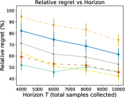
(a) Relative regret

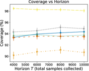
(b) Coverage

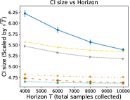
(c) CI size

Figure 3: Results for the two-sample IV LATE estimation task (Example 2) for a nonlinear causal model where MLPs are used for nuisance estimation (error bars denote $95\%$ CIs). In this case, significant bias is incurred due to nuisance estimation even at large horizons. The online data collection policies outperform the fixed policy in terms of regret and coverage.

The labels $\text{etc}\_{x}$ and $\text{etg}\_{x}$ in the plots (Fig. 3) refer to the ETC and ETG policies with exploration $e=x$. For the ETG policies, we set the batch size $S$ such that $S/(T(1-e))=0.1$. Thus, the estimate of the oracle simplex $\widehat{k}_{t}$ is updated every $10\%$ of the horizon $T$ after exploration. The label fixed refers to a fixed policy that queries each data source equally with $\kappa_{T}=[0.5,0.5]^{\top}$. We use oracle-$\widehat{\eta}$ to denote the oracle policy that uses estimated nuisance functions (instead of the true nuisances $\eta^{*}$). For computational reasons, we retrain the nuisance estimators in batches (rather than after every time step).

In terms of relative regret (Fig. 3(a)), we observe that even oracle-$\widehat{\eta}$ has $\approx 50\%$ relative regret, showing substantial bias due to nuisance estimation. The online policies (ETC and ETG) outperform the fixed policy, with ETG having similar relative regret as oracle-$\widehat{\eta}$. Moreover, etg_$0.1$ outperforms etc_$0.1$, demonstrating the advantage of repeatedly updating the estimate of the oracle simplex. In terms of coverage (Fig. 3(b)), the online policies outperform the fixed policy, and get close to the nominal coverage of $95\%$ at large horizons. Finally, we observe that the size of the confidence intervals (Fig. 3(c)) for the etg policies is significantly smaller than the confidence intervals (CIs) of etc and oracle-$\widehat{\eta}$.

We also perform experiments for Examples 2, 3, and 4 with synthetic data generated from linear causal models (see Appendix H.2), observing that the ETC and ETG policies have lower relative regret than the fixed policy in all cases. Since we use correctly specified parametric nuisance estimators, the bias due to nuisance estimation is substantially lower in this case, with the ETG policy achieving nearly zero relative regret at large horizons.

7.2 Real-world data

JTPA dataset.

The National Job Training Partnership Act (JTPA) study examines the effect of a job training program on future earnings and has been analyzed in several prior works (Glynn and Kashin, 2018; Donald et al., 2014; Abadie et al., 2002; Bloom et al., 1997). The data follows the IV causal model (see Example 2 and Fig. 1(a)) with a binary IV $Z$, binary treatment $X$, a vector of covariates $W$, and a real-valued outcome $Y$. We use the dataset from Glynn and Kashin (2019), which contains $N=4384$ samples. In this dataset, $Z$ indicates whether the individual was randomly offered training, $X$ denotes program participation, $Y$ denotes future earnings, and $W$ contains six covariates which include variables like race and age. We simulate the two-sample LATE estimation setting in Example 2 with ${\mathcal{D}}=\left(\widehat{{\mathbb{P}}}_{N}(W,Z,Y),\widehat{{\mathbb{P}}}_{N}(W,Z,X)\right)$, where $\widehat{{\mathbb{P}}}_{N}$ denotes the empirical distribution over the $N$ samples. The true LATE and oracle simplex are computed on the full dataset with MLP-based nuisance estimators and cross-fitting with $k=2$ folds (Chernozhukov et al., 2018), averaged over $2000$ runs. We compare the scaled MSE ($T\times\text{MSE}$) of our proposed policies with a fixed policy that queries both data sources uniformly with $\kappa_{T}=[0.5,0.5]^{\top}$ (Fig. 4(a)). We observe that the MSE of the fixed policy is nearly twice as large as the oracle policy. By contrast, we see that the ETC and ETG policies match the oracle policy at all horizons.

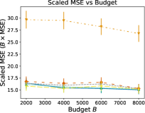
(a) JTPA data

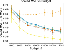
(b) COPD data

Figure 4: Results on two real-world causal effect estimation tasks (error bars denote $95\%$ CIs). In both cases, we observe that the online data collection policies outperform the fixed policy (as the budget increases).

COPD dataset.

We test our strategies on datasets used to evaluate the effect of chronic obstructive pulmonary disease (COPD) on the development of herpes zoster (HZ) (Lin and Chen, 2014). We use the dataset released by Yang and Ding (2019), which follows the setting of Example 4 (where an unconfounded dataset is combined with a confounded dataset). The treatment $X\in\{0,1\}$ and outcome $Y\in\{0,1\}$ denote the presence of COPD and HZ, respectively. We have two datasets: (i) The validation dataset with $N_{\text{val}}=1148$ samples of $(U,W,X,Y)$ and (ii) The main dataset with $N_{\text{main}}=42430$ samples of $(W,X,Y)$. The covariates $W$ include variables like age, presence of liver disease, etc. and $U$ includes variables like cigarette and alcohol consumption which are known to be important confounders (but are missing in the main dataset).

To test our methods, we use ${\mathcal{D}}=(\widehat{{\mathbb{P}}}_{\text{val}}(U,W,X,Y),\widehat{{\mathbb{P}}}_{\text{main}}(W,X,Y))$, where $\widehat{{\mathbb{P}}}_{\text{val}}$ and $\widehat{{\mathbb{P}}}_{\text{main}}$ denote the empirical distributions over the validation and main datasets. We apply a cost structure of $c=[4,1]$, i.e., a query to the validation dataset costs four times that of the main dataset. The dataset contains the propensity scores (not the covariates). Since propensity scores suffice for removing confounding bias (Hernán and Robins, 2010, Sec. 15.2), we use them as covariates with linear nuisance estimators. The true ATE and oracle simplex are computed on the full dataset using cross-fitting with $k=2$ folds. We compare the regret of our proposed adaptive policies to that of a fixed policy that only queries the first data source with $\kappa_{T}=[1,0]^{\top}$ (Fig. 4(b)). We observe that both the fixed and online policies have higher MSE than the oracle at all budgets. At smaller budget sizes, we do not observe a significant difference with the fixed policy. However, as the budget increases, we observe that the online policies substantially outperform the fixed policy and are much closer to the oracle.

8 Conclusion

Our work presents a semiparametric framework for statistical inference that accounts for sequential data collection decisions. Aiming to efficiently estimate a given target parameter, we present two online data collection policies, OMS-ETC and OMS-ETG, and prove that both achieve zero asymptotic regret relative to the oracle policy. One limitation of our theoretical results is that they do not distinguish between OMS-ETC and OMS-ETG. Overcoming this limitation would potentially require higher-order or finite-sample analysis. Another limitation is that our results hold pointwise rather than uniformly in the probability space, which could lead to different optimal rates (e.g., in multi-armed bandits, better minimax optimal rates are achieved when considering pointwise or instance-dependent bounds (Lattimore and Szepesvári, 2020, Ch. 16)). In future work, we aim to extend our work to the contextual selection setting where the data source can be selected based on variables revealed in the same time step. We also aim to extend our analysis beyond scalar parameters to targets that are multivariate or nonparametric as well as parameters identified by conditional moment restrictions.

Appendix A Proof of consistency

Proposition 8 (MDS SLLN [Csörgö, 1968, Theorem 1]).

Let $\{X_{n},n\in\mathbb{N}\}$ be a martingale difference sequence (MDS) and $b_{1}<b_{2}<\ldots\rightarrow\infty$ be a non-decreasing sequence such that $\sum_{i=1}^{\infty}b^{-2}_{i}{\mathbb{E}}[X^{2}_{i}]<\infty$. Then $b^{-1}_{n}\sum_{i=1}^{n}X_{i}\overset{a.s.}{\to}0$.

Corollary 1.

Let $\{X_{n},n\in\mathbb{N}\}$ be a MDS with $\sup_{n}{\mathbb{E}}[X^{2}_{n}]<\infty$. Then $n^{-1}\sum_{i=1}^{n}X_{i}\overset{a.s.}{\to}0$.

Proof.

Apply Prop. 8 with $b_{i}=i$. ∎

Proposition 9 (Convergence of moments [Billingsley, 1995, Page 338]).

Let $r$ be a positive integer. If $X_{n}\overset{d}{\to}X$ and $\sup_{n}{\mathbb{E}}[|X_{n}|^{r+\epsilon}]<\infty$, where $\epsilon>0$, then ${\mathbb{E}}[|X|^{r}]<\infty$, and ${\mathbb{E}}[X_{n}^{r}]\to{\mathbb{E}}[X^{r}]$.

Lemma 4.

Let $(X_{t})_{t=1}^{\infty}$ be a sequence of non-negative random variables with (i) $X_{t}\overset{p}{\to}0$ and (ii) $\exists\delta>0$ such that $\sup_{t}{\mathbb{E}}[X_{t}^{1+\delta}]<\infty$. Then $T^{-1}\sum_{t=1}^{T}X_{t}\overset{p}{\to}0$.

Proof.

By Markov’s inequality, for any $\epsilon>0$,

$${\mathbb{P}}\left(\frac{1}{T}\sum_{t=1}^{T}X_{t}>\epsilon\right) \leq\frac{\sum_{t=1}^{T}{\mathbb{E}}[X_{t}]}{T\epsilon}$$

$$\leq\frac{o(T)}{T\epsilon}=o(1),$$ (7)

where (7) follows because ${\mathbb{E}}[\|\widehat{\eta}_{t-1}-\eta^{*}\|]=o(1)$ (by Conditions (i, ii) and Prop. 9). ∎

Lemma 5 (ULLN).

Suppose that $a_{t}(\theta,\eta):=a(X_{t};\theta,\eta)$ satisfies Property 1. Let $a_{*}(\theta,\eta)={\mathbb{E}}[a(X_{t};\theta,\eta)]$ and $s_{t}\in\{0,1\}$ be a $H_{t-1}$-measurable binary random variable. Then the following uniform law of large numbers (ULLN) holds:

$$\sup_{\theta\in\Theta}\left|\frac{1}{T}\sum_{t=1}^{T}s_{t}\left\{a_{t}(\theta,\widehat{\eta}_{t-1})-a_{*}(\theta,\eta^{*})\right\}\right|\overset{p}{\to}0.$$

Proof.

We prove the ULLN by a covering number argument [Tauchen, 1985, Lemma 1]. Let $\left\{\theta_{k}\right\}_{k=1}^{K}$ be a minimal $\delta$-cover of $\Theta$ and ${\mathcal{B}}_{\delta}(\theta_{k})$ denotes the $\delta$-ball around $\theta_{k}$. By compactness of $\Theta$ (Assumption 3b), $K$ is finite. For the rest of the proof, for any $\theta\in\Theta$, let $\theta_{k}$ denote the element of the $\delta$-cover such that $\theta\in{\mathcal{B}}_{\delta}(\theta_{k})$.

By the triangle inequality,

$$\sup_{\theta\in\Theta} \left|\frac{1}{T}\sum_{t=1}^{T}s_{t}\left\{a_{t}(\theta,\widehat{\eta}_{t-1})-a_{*}(\theta,\eta^{*})\right\}\right|$$

$$\leq\begin{aligned} &\sup_{\theta}\left|\frac{1}{T}\sum_{t=1}^{T}s_{t}\left\{a_{t}(\theta,\widehat{\eta}_{t-1})-a_{t}(\theta_{k},\widehat{\eta}_{t-1})\right\}\right|+\max_{k\in[K]}\left|\frac{1}{T}\sum_{t=1}^{T}s_{t}\left\{a_{t}(\theta_{k},\widehat{\eta}_{t-1})-a_{*}(\theta_{k},\eta^{*})\right\}\right|+\\ &\max_{k\in[K]}\frac{1}{T}\sum_{t=1}^{T}s_{t}\left|a_{*}(\theta_{k},\eta^{*})-a_{*}(\theta,\eta^{*})\right|\end{aligned}$$

$$\leq\begin{aligned} &\underbrace{\frac{1}{T}\sum_{t=1}^{T}\sup_{\theta}\left|a_{t}(\theta,\widehat{\eta}_{t-1})-a_{t}(\theta_{k},\widehat{\eta}_{t-1})\right|}_{\text{T1}}+\underbrace{\max_{k\in[K]}\left|\frac{1}{T}\sum_{t=1}^{T}s_{t}\left\{a_{t}(\theta_{k},\widehat{\eta}_{t-1})-a_{*}(\theta_{k},\eta^{*})\right\}\right|}_{\text{T2}}+\\ &\underbrace{\max_{k\in[K]}\left|a_{*}(\theta_{k},\eta^{*})-a_{*}(\theta,\eta^{*})\right|}_{\text{T3}},\end{aligned}$$ (8)

where (8) follows because $s_{t}\in\{0,1\}$. Next, we show that all three terms are $o_{\text{p}}(1)$.

Term (T1).

$$\frac{1}{T}\sum_{t=1}^{T}\sup_{\theta}\left|a_{t}(\theta,\widehat{\eta}_{t-1})-a_{t}(\theta_{k},\widehat{\eta}_{t-1})\right| =\frac{1}{T}\sum_{t=1}^{T}\delta\left|L(X_{t})\right|$$ (9)

$$=\delta{\mathbb{E}}[L(X_{t})]+o_{\text{a.s.}}(1)$$ (10)

$$\leq\sqrt{L}\delta+o_{\text{a.s.}}(1),$$ (11)

where (9) and (11) follow by Property 1(ii) (Lipschitzness) and (10) follows by Corollary 1. Therefore, for any $\epsilon>0$ and a small enough $\delta$, the term T1 will be less than $\epsilon$ eventually.

Term (T2).

For any $k\in[K]$, by the triangle inequality,

$$\left|\frac{1}{T}\sum_{t}s_{t}\left[a_{t}(\theta_{k},\widehat{\eta}_{t-1})-a_{*}(\theta_{k},\eta^{*})\right]\right|$$

$$\leq\begin{aligned} &\underbrace{\left|\frac{1}{T}\sum_{t}s_{t}\left[a_{t}(\theta_{k},\eta^{*})-a_{*}(\theta_{k},\eta^{*})\right]\right|}_{:=a}+\\ &\underbrace{\left|\frac{1}{T}\sum_{t}s_{t}\left[a_{t}(\theta_{k},\widehat{\eta}_{t-1})-a_{t}(\theta_{k},\eta^{*})-{\mathbb{E}}_{t-1}[a_{t}(\theta_{k},\widehat{\eta}_{t-1})-a_{t}(\theta_{k},\eta^{*})]\right]\right|}_{:=b}+\\ &\underbrace{\left|\frac{1}{T}\sum_{t}s_{t}{\mathbb{E}}_{t-1}[a_{t}(\theta_{k},\widehat{\eta}_{t-1})-a_{t}(\theta_{k},\eta^{*})]\right|}_{:=c}.\end{aligned}$$

The term a above is a martingale difference sequence (MDS). By Property 1(i) and Corollary 1, this term is $o_{\text{a.s.}}(1)$. The term b above is also a MDS. For $D_{t}=a_{t}(\theta_{k},\widehat{\eta}_{t-1})-a_{t}(\theta_{k},\eta^{*})$,

$${\mathbb{E}}[s_{t}(D_{t}-{\mathbb{E}}_{t-1}[D_{t}])^{2}] \leq{\mathbb{E}}[(D_{t}-{\mathbb{E}}_{t-1}[D_{t}])^{2}]$$ (12)

$$\leq{\mathbb{E}}[D_{t}^{2}]$$

$$\leq{\mathbb{E}}[{\mathbb{E}}_{t-1}[D_{t}^{2}]]$$

$$\leq L{\mathbb{E}}[\|\widehat{\eta}_{t-1}-\eta^{*}\|^{2}]$$ (13)

$$<\infty,$$ (14)

where (12) follows because $s_{t}\in\{0,1\}$, (13) by Property 1(ii), and (14) by Property 1(iv). Thus, by Corollary 1, this term is also $o_{\text{a.s.}}(1)$. For term c, we have

$$\left|\frac{1}{T}\sum_{t}s_{t}{\mathbb{E}}_{t-1}[a_{t}(\theta_{k},\widehat{\eta}_{t-1})-a_{t}(\theta_{k},\eta^{*})]\right| \leq\frac{1}{T}\sum_{t}{\mathbb{E}}_{t-1}[|a_{t}(\theta_{k},\widehat{\eta}_{t-1})-a_{t}(\theta_{k},\eta^{*})|]$$ (15)

$$\leq\frac{1}{T}\sum_{t}\sqrt{{\mathbb{E}}_{t-1}[|a_{t}(\theta_{k},\widehat{\eta}_{t-1})-a_{t}(\theta_{k},\eta^{*})|^{2}]}$$

$$\leq\frac{\sqrt{L}}{T}\sum_{t}\|\widehat{\eta}_{t-1}-\eta^{*}\|$$ (16)

$$=o_{p}(1),$$ (17)

where (15) follows because $s_{t}\in\{0,1\}$, (16) by Property 1(ii), and (17) by Lemma 4. This allows us to show that term T2 is $o_{\text{p}}(1)$:

$$\max_{k\in[K]}\left|\frac{1}{T}\sum_{t=1}^{T}s_{t}\left\{a_{t}(\theta_{k},\widehat{\eta}_{t-1})-a_{*}(\theta_{k},\eta^{*})\right\}\right| \leq\sum_{k\in[K]}\left|\frac{1}{T}\sum_{t=1}^{T}s_{t}\left\{a_{t}(\theta_{k},\widehat{\eta}_{t-1})-a_{*}(\theta_{k},\eta^{*})\right\}\right|$$

$$=o_{\text{p}}(1),$$

where the last line follows because $K$ is finite.

Term (T3).

By Property 1(ii),

$$\max_{k\in[K]}\left|a_{*}(\theta_{k},\eta^{*})-a_{*}(\theta,\eta^{*})\right|\leq{\mathbb{E}}[L(X_{t})]\delta\leq\sqrt{L}\delta.$$

Thus, for any $\epsilon>0$ and a small enough $\delta$, the term T3 will be less than $\epsilon$. ∎

Proposition 10.

Suppose that (i) $f_{t}(\theta,\eta):=f(X_{t};\theta,\eta)$ and $g_{t}(\theta,\eta):=g(X_{t};\theta,\eta)$ satisfy Property 1; and (ii) (Boundedness) $\forall(\theta,\eta),|f_{t}(\theta,\eta)|_{\infty}\leq H$ and $|g_{t}(\theta,\eta)|_{\infty}\leq H$ for some constant $H<\infty$. Then, $f_{t}(\theta,\eta)g_{t}(\theta,\eta)$ satisfies Property 1.

Proof.

We show that the conditions of Property 1 hold for $a_{t}(\theta,\eta)=f_{t}(\theta,\eta)g_{t}(\theta,\eta)$.

Property 1(i).

For any $\theta,\eta$,

$${\mathbb{E}}\left[|a_{t}(\theta,\eta)|^{2+\delta}\right] ={\mathbb{E}}\left[|f_{t}(\theta,\eta)g_{t}(\theta,\eta)|^{2+\delta}\right]$$

$$\leq H^{4+2\delta}$$

$$<\infty.$$

Property 1(ii).

We have that $\forall\theta,\theta^{\prime}\in\Theta,\forall\eta\in{\mathcal{T}}$,

$$|a_{t}(\theta^{\prime},\eta)-a_{t}(\theta,\eta)| =|f_{t}(\theta^{\prime},\eta)g_{t}(\theta^{\prime},\eta)-f_{t}(\theta,\eta)g_{t}(\theta,\eta)|$$

$$=|f_{t}(\theta^{\prime},\eta)(g_{t}(\theta^{\prime},\eta)-g_{t}(\theta,\eta)+g_{t}(\theta,\eta))-f_{t}(\theta,\eta)g_{t}(\theta,\eta)|$$

$$=|f_{t}(\theta^{\prime},\eta)(g_{t}(\theta^{\prime},\eta)-g_{t}(\theta,\eta))+g_{t}(\theta,\eta)(f_{t}(\theta^{\prime},\eta)-f_{t}(\theta,\eta))|$$

$$\leq L(X_{t})(|f_{t}(\theta^{\prime},\eta)|+|g_{t}(\theta,\eta)|)\|\theta-\theta^{\prime}\|,$$ (18)

where (18) follows by Condition (i). Furthermore, by Condition (ii), we have

$${\mathbb{E}}[(L(X_{t})(|f_{t}(\theta^{\prime},\eta)|+|g_{t}(\theta,\eta)|))^{2}] \leq 4H^{2}{\mathbb{E}}[L(X_{t})^{2}]$$

$$<\infty.$$

Next, by Conditions (i, ii), we have that $\forall\theta\in\Theta,\forall\eta,\eta^{\prime}\in{\mathcal{T}}$,

$${\mathbb{E}}[(a_{t}(\theta,\eta) -a_{t}(\theta,\eta^{\prime}))^{2}]={\mathbb{E}}[(f_{t}(\theta,\eta)g_{t}(\theta,\eta)-f_{t}(\theta,\eta^{\prime})g_{t}(\theta,\eta^{\prime}))^{2}]$$

$$={\mathbb{E}}[(f_{t}(\theta,\eta)(g_{t}(\theta,\eta)-g_{t}(\theta,\eta^{\prime}))+g_{t}(\theta,\eta^{\prime})(f_{t}(\theta,\eta)-f_{t}(\theta,\eta^{\prime})))^{2}]$$

$$=\begin{aligned} &{\mathbb{E}}[f^{2}_{t}(\theta,\eta)(g_{t}(\theta,\eta)-g_{t}(\theta,\eta^{\prime}))^{2}]+{\mathbb{E}}[g^{2}_{t}(\theta,\eta^{\prime})(f_{t}(\theta,\eta)-f_{t}(\theta,\eta^{\prime}))^{2}]\\ &+2{\mathbb{E}}[f_{t}(\theta,\eta)g_{t}(\theta,\eta^{\prime})(g_{t}(\theta,\eta)-g_{t}(\theta,\eta^{\prime}))(f_{t}(\theta,\eta)-f_{t}(\theta,\eta^{\prime})]\end{aligned}$$

$$\leq\begin{aligned} 2H^{2}L\|\eta-\eta^{\prime}\|^{2}+2H^{2}{\mathbb{E}}[|(g_{t}(\theta,\eta)-g_{t}(\theta,\eta^{\prime}))(f_{t}(\theta,\eta)-f_{t}(\theta,\eta^{\prime})|]\end{aligned}$$

$$\leq\begin{aligned} 2H^{2}L\|\eta-\eta^{\prime}\|^{2}+2H^{2}\sqrt{{\mathbb{E}}[(g_{t}(\theta,\eta)-g_{t}(\theta,\eta^{\prime}))^{2}]{\mathbb{E}}[(f_{t}(\theta,\eta)-f_{t}(\theta,\eta^{\prime}))^{2}]}\end{aligned}$$

$$\leq\begin{aligned} 4H^{2}L\|\eta-\eta^{\prime}\|^{2}\end{aligned},$$

completing the proof. ∎

Before presenting the proof of Prop. 1, we define some additional notation. Recall that $\widehat{\theta}_{T}=\arg\min_{\theta\in\Theta}\widehat{Q}_{T}(\theta,(\widehat{\eta}_{t-1})_{t=1}^{T})$ (see Eq. 2) and the moment conditions have the following form (see Eq. 1):

$$g_{t}(\theta,\eta)=m(s_{t})\odot\tilde{g}_{t}(\theta,\eta),$$

where $m:\{0,1\}^{\left|{\mathcal{D}}\right|}\mapsto\{0,1\}^{M}$ is a fixed known function that determines which moments get selected based on the selection vector $s_{t}$. For some $\kappa\in\Delta_{{\mathcal{D}}}$ and $s_{t}\overset{\text{i.i.d.}}{\sim}\text{Multinouilli}(\kappa)$, we define the following matrices:

$$m_{G}(\kappa) :={\mathbb{E}}[\underbrace{[m(s_{t}),\ldots,m(s_{t})]}_{D\,\text{times}}]\in[0,1]^{M\times D},$$ (19)

$$m_{\Omega}(\kappa) :={\mathbb{E}}\left[m(s_{t})m(s_{t})^{\top}\right]\in[0,1]^{M\times M}.$$ (20)

Proposition 1 (Consistency).

Suppose that (i) Assumption 3 holds; (ii) $\forall i\in[M],\psi^{(i)}$ satisfies Property 1; (iii) $\forall(i,j)\in[M]^{2},\psi^{(i)}\psi^{(j)}$ satisfies Property 1. Then $\widehat{\beta}_{T}\overset{p}{\to}\beta^{*}$.

Proof.

We define the following matrices:

$$\widehat{\Omega}_{T}(\theta) :=\frac{1}{T}\sum_{t}g_{t}(\theta,\widehat{\eta}_{t-1})g^{\top}_{t}(\theta,\widehat{\eta}_{t-1})$$

$$\Omega_{T}(\theta) :=\frac{1}{T}\sum_{t}{\mathbb{E}}_{t-1}\left[g_{t}(\theta,\eta^{*})g^{\top}_{t}(\theta,\eta^{*})\right]$$

$$=\left[\frac{1}{T}\sum_{t}m(s_{t})m(s_{t})^{\top}\right]\odot{\mathbb{E}}[\tilde{g}_{t}(\theta,\eta^{*})\tilde{g}_{t}^{\top}(\theta,\eta^{*})]$$

$$=m_{\Omega}(\kappa_{T})\odot{\mathbb{E}}[\tilde{g}_{t}(\theta,\eta^{*})\tilde{g}_{t}^{\top}(\theta,\eta^{*})].$$

We define the empirical and population versions of the GMM objective:

$$\widehat{Q}_{T}(\theta,(\widehat{\eta}_{t-1})_{t=1}^{T}): =\left[\frac{1}{T}\sum_{t=1}^{T}g_{t}(\theta,\widehat{\eta}_{t-1})\right]^{\top}\widehat{W}_{T}\left[\frac{1}{T}\sum_{t=1}^{T}g_{t}(\theta,\widehat{\eta}_{t-1})\right],$$

$$\bar{Q}_{T}(\theta): =\left[\frac{1}{T}\sum_{t=1}^{T}{\mathbb{E}}_{t-1}\left[g_{t}(\theta,\eta^{*})\right]^{\top}\right]W_{T}\left[\frac{1}{T}\sum_{t=1}^{T}{\mathbb{E}}_{t-1}\left[g_{t}(\theta,\eta^{*})\right]\right]$$

$$=\left[\left(\frac{1}{T}\sum_{t=1}^{T}m(s_{t})\right)\odot g_{*}(\theta)\right]^{\top}W_{T}\left[\left(\frac{1}{T}\sum_{t=1}^{T}m(s_{t})\right)\odot g_{*}(\theta)\right]$$

where $g_{*}(\theta):={\mathbb{E}}\left[\tilde{g}_{t}(\theta,\eta^{*})\right]$. For the one-step GMM estimator, denoted by $\widehat{\theta}_{T}^{(\text{os})}$, we use $\widehat{W}_{T}=W_{T}=I\,(\text{identity})$. For the two-step GMM estimator, we use $\widehat{W}_{T}=\widehat{\Omega}_{T}(\widehat{\theta}_{T}^{(\text{os})})^{-1}$ and $W_{T}=\Omega_{T}(\theta^{*})^{-1}$.

By Assumption 3(a), the true parameter $\theta^{*}$ uniquely minimizes the population objective: $\theta^{*}=\arg\min_{\theta\in\Theta}\bar{Q}_{T}(\theta)$. By the same argument as Newey and McFadden [1994, Thm. 2.1], if $\sup_{\theta\in\Theta}|\widehat{Q}_{T}(\theta,(\widehat{\eta}_{t-1})_{t=1}^{T})-\bar{Q}_{T}(\theta)|\overset{p}{\to}0$, then $\widehat{\theta}_{T}\overset{p}{\to}\theta^{*}$. Thus, to show consistency, we prove the uniform convergence of $\widehat{Q}_{T}(\theta,(\widehat{\eta}_{t-1})_{t=1}^{T})$. By the triangle inequality,

$$\left|\widehat{Q}_{T}(\theta,(\widehat{\eta}_{t-1})_{t=1}^{T})-\bar{Q}_{T}(\theta)\right|\leq F_{T}(\theta)^{2}\|\widehat{W}_{T}\|^{2}+2\left\|g_{*}(\theta)\right\|F_{T}(\theta)\|\widehat{W}_{T}\|+\left\|g_{*}(\theta)\right\|^{2}\|\widehat{W}_{T}-W_{T}\|,$$

where $F_{T}(\theta):=\|T^{-1}\sum_{t=1}^{T}\left[g_{t}(\theta,\widehat{\eta}_{t-1})\\ -m(s_{t})\odot g_{*}(\theta)\right]\|$. We prove the uniform convergence of $F_{T}(\theta)$ by applying Lemma 5 to every element of $g_{t}(\theta,\widehat{\eta}_{t-1})$ along with the union bound. For any $\epsilon>0$,

$${\mathbb{P}}\left(\sup_{\theta\in\Theta}F_{T}(\theta)<\epsilon\right) \geq{\mathbb{P}}\left(\sup_{\theta\in\Theta}\sum_{i=1}^{M}\left|\frac{1}{T}\sum_{t=1}^{T}\left[g_{t,i}(\theta,\widehat{\eta}_{t-1})-m_{i}(s_{t})\odot g_{*}(\theta)_{i}\right]\right|<\epsilon\right)$$

$$\geq 1-\sum_{i=1}^{M}{\mathbb{P}}\left(\sup_{\theta\in\Theta}\left|\frac{1}{T}\sum_{t=1}^{T}\left[g_{t,i}(\theta,\widehat{\eta}_{t-1})-m_{i}(s_{t})\odot g_{*}(\theta)_{i}\right]\right|>\frac{\epsilon}{M}\right)$$ (21)

$$\geq 1-o_{\text{p}}(1),$$ (22)

where (21) follows by the union bound, and (22) by Lemma 5. For the one-step GMM estimator, we have $\widehat{W}_{T}=W_{T}=I$ (identity) and so $\|\widehat{W}_{T}-W_{T}\|\overset{p}{\to}0$ holds trivially. Therefore, $\widehat{\theta}^{\text{(os)}}_{T}\overset{p}{\to}\theta^{*}$. For the two-step estimator, we need to show that $\|\widehat{W}_{T}-W_{T}\|\overset{p}{\to}0$. For all $(i,j)\in[M]^{2}$ and any $\epsilon>0$,

$${\mathbb{P}}\left(\sup_{\theta\in\Theta}\left|\widehat{\Omega}_{T}(\theta)_{i,j}-\Omega_{T}(\theta)_{i,j}\right|>\epsilon\right) \to 0,$$ (23)

$$\therefore\,{\mathbb{P}}\left(\left|\widehat{\Omega}_{T}(\widehat{\theta}^{\text{(os)}}_{T})_{i,j}-\Omega_{T}(\widehat{\theta}^{\text{(os)}}_{T})_{i,j}\right|>\epsilon\right) \to 0,$$

$$\therefore\,{\mathbb{P}}\left(\left|\widehat{\Omega}_{T}(\widehat{\theta}^{\text{(os)}}_{T})_{i,j}-\Omega_{T}(\theta^{*})_{i,j}\right|>\epsilon\right) \to 0,$$ (24)

$$\therefore\,{\mathbb{P}}\left(\left|(\widehat{W}_{T})_{i,j}-(W_{T})_{i,j}\right|>\epsilon\right) \to 0,$$ (25)

$$\therefore\,{\mathbb{P}}\left(\left\|\widehat{W}_{T}-W_{T}\right\|>\epsilon\right) \to 0,$$

where (23) follows by Lemma 5 and Condition (iii); (24) follows because $\widehat{\theta}^{\text{(os)}}_{T}\overset{p}{\to}\theta^{*}$; and (25) by continuity of the matrix inverse. Therefore, $\widehat{\theta}_{T}\overset{p}{\to}\theta^{*}$. Since $\widehat{\beta}_{T}=f_{\text{tar}}(\widehat{\theta}_{T})$, by continuity of $f_{\text{tar}}$ (Assumption 3c), we have $\widehat{\beta}_{T}\overset{p}{\to}\beta^{*}$. ∎

Appendix B Proof of asymptotic normality

Proposition 11 (Martingale CLT [Häusler and Luschgy, 2015, Thm. 6.23]).

Let $\{X_{i},{\mathcal{F}}_{i},1\leq i\leq n\}$ be a martingale difference sequence and let ${\mathcal{F}}_{\infty}:=\sigma\left(\bigcup_{i=1}^{\infty}{\mathcal{F}}_{i}\right)$. Let $\gamma^{2}$ be an a.s. finite random variable. Suppose that (i) (Square integrable) $\forall i,{\mathbb{E}}[X^{2}_{i}]<\infty$; (ii) (Conditional Lindeberg) $\forall\epsilon>0$, $n^{-1}\sum_{i=1}^{n}{\mathbb{E}}\left[X^{2}_{i}\mathbbm{1}\left(|X_{i}|>\epsilon\sqrt{n}\right)|{\mathcal{F}}_{i-1}\right]\overset{p}{\to}0$, and (ii) (Convergence of conditional variance) $n^{-1}\sum_{i=1}^{n}{\mathbb{E}}\left[X^{2}_{i}|{\mathcal{F}}_{i-1}\right]\overset{p}{\to}\gamma^{2}$ for some random variable $\gamma$. Let $Z\sim N(0,1)$ be a standard Gaussian independent of ${\mathcal{F}}_{\infty}$. Then

$$\frac{1}{\sqrt{n}}\sum_{i=1}^{n}X_{i}\overset{d}{\to}\gamma Z\,\,\,{\mathcal{F}}_{\infty}\text{-stably},$$

where the random variable $\gamma Z$ is a mixture of centered normal distributions with the characteristic function $\varphi(t)={\mathbb{E}}_{\gamma}[-\gamma^{2}t^{2}/2]$. If $\gamma$ is a.s. constant, then

$$\frac{1}{\sqrt{n}}\sum_{i=1}^{n}X_{i}\overset{d}{\to}{\mathcal{N}}(0,\gamma^{2}).$$

Proposition 12 (Properties of stable convergence [Häusler and Luschgy, 2015, Thm. 3.18]).

Assume that $X_{n}\overset{d}{\to}X\,\,{\mathcal{G}}\text{-stably}$. Let $Y_{n}$ and $Y$ be random variables. (a) If $Y_{n}\overset{p}{\to}Y$ and $Y$ is ${\mathcal{G}}$-measurable, then $(Y_{n},X_{n})\to(X,Y)\,\,{\mathcal{G}}\text{-stably}$. (b) If $g$ is a measurable and continuous function, then $g(X_{n})\to g(X)\,\,{\mathcal{G}}\text{-stably}$.

Corollary 2 (Cramer-Slutsky).

Assume that $X_{n}\overset{d}{\to}X\,\,{\mathcal{G}}\text{-stably}$. Let $Y_{n}$ and $Y$ be random variables. If $Y_{n}\overset{p}{\to}Y$ and $Y$ is ${\mathcal{G}}$-measurable, then $Y_{n}X_{n}\overset{d}{\to}YX\,\,{\mathcal{G}}\text{-stably}$.

Proof.

Apply Prop. 12 with the function $g(X,Y)=XY$. ∎

Proposition 13 (Cramer-Wold device [Häusler and Luschgy, 2015, Cor. 3.19]).

If $u^{\top}Y_{n}\overset{d}{\to}u^{\top}Y\,\,{\mathcal{G}}\text{-stably}$ for every $u\in{\mathbb{R}}^{d}$, then $Y_{n}\overset{d}{\to}Y\,\,{\mathcal{G}}\text{-stably}$.

Lemma 6.

Let $(X_{t})_{t=1}^{\infty}$ be a sequence of non-negative random variables such that (i) $\sup_{t}{\mathbb{E}}[X^{1+\delta}_{t}]<\infty$ and (ii) $X_{t}=o_{\text{p}}(t^{-1/2})$. Then

$$\frac{1}{\sqrt{T}}\sum_{i=1}^{T}X_{t}=o_{\text{p}}(1).$$

Proof.

By Markov’s inequality, for any $\epsilon>0$,

$${\mathbb{P}}\left(\frac{1}{\sqrt{T}}\sum_{i=1}^{T}X_{t}>\epsilon\right) \leq\frac{\sum_{t}{\mathbb{E}}[X_{t}]}{\sqrt{T}\epsilon}$$

$$=\frac{o(\sqrt{T})}{\sqrt{T}\epsilon}$$ (26)

$$=o(1),$$

where (26) follows because ${\mathbb{E}}[X_{t}]=o(t^{-1/2})$ (by Conditions (i, ii) and Prop. 9). ∎

Proposition 2 (Asymptotic normality).

Suppose that (i) Conditions of Prop. 1 hold; (ii) Assumptions 4 and 5 hold; and (iii) $\forall i\in[M],j\in[D],\partial_{\theta_{j}}\left[\psi^{(i)}_{t}(\theta,\eta)\right]$ satisfies Property 1. Then $\widehat{\beta}_{T}$ converges to a mixture of normals, where the mixture is over $\kappa_{\infty}$:

$$\sqrt{T}(\widehat{\beta}_{T}-\beta^{*}) \overset{d}{\to}{\mathcal{N}}_{\kappa_{\infty}}\left(0,V_{*}(\kappa_{\infty})\right),$$

where $V_{*}(\kappa)$ is a constant that depends on $(\theta^{*},\eta^{*},\kappa)$. If $\kappa_{\infty}$ is almost surely constant, then $\widehat{\beta}_{T}$ is asymptotically normal.

Proof.

Recall that $\widehat{\theta}_{T}=\arg\min_{\theta\in\Theta}\widehat{Q}_{T}(\theta,(\widehat{\eta}_{t-1})_{t=1}^{T})$ (see Eq. 2). For the two-step GMM estimator, by first-order optimality, we have

$$\sqrt{T}(\widehat{\theta}_{T}-\theta^{*})=-\left[\widehat{G}_{T}^{\top}(\widehat{\theta}_{T})\widehat{\Omega}(\widehat{\theta}^{(\text{os})}_{T})^{-1}\widehat{G}_{T}(\tilde{\theta})\right]^{-1}\widehat{G}_{T}^{\top}(\widehat{\theta}_{T})\widehat{\Omega}(\widehat{\theta}^{(\text{os})}_{T})^{-1}\frac{1}{\sqrt{T}}\sum_{t=1}^{T}g_{t}(\theta^{*},\widehat{\eta}_{t-1}),$$ (27)

where $\widehat{\theta}^{(\text{os})}_{T}$ is the one-step GMM estimator, $\tilde{\theta}$ is a point on the line-segment joining $\widehat{\theta}_{T}$ and $\theta^{*}$,

$$\widehat{G}_{T}(\theta) =\frac{1}{T}\sum_{t=1}^{T}\frac{\partial g_{t}(\theta,\widehat{\eta}_{t-1})}{\partial\theta}$$

$$=\frac{1}{T}\sum_{t=1}^{T}\frac{\partial(m(s_{t})\odot\tilde{g}_{t}(\theta,\widehat{\eta}_{t-1}))}{\partial\theta}$$

$$=\frac{1}{T}\sum_{t=1}^{T}\left(\underbrace{\left[m(s_{t}),m(s_{t}),\ldots,m(s_{t})\right]}_{D\,\text{times}}\odot\left[\frac{\partial\tilde{g}_{t}(\theta,\widehat{\eta}_{t-1})}{\partial\theta}\right]\right),$$

$$=\frac{1}{T}\sum_{t=1}^{T}\left(m_{G}(s_{t})\odot\left[\frac{\partial\tilde{g}_{t}(\theta,\widehat{\eta}_{t-1})}{\partial\theta}\right]\right),\,\text{and}$$

$$\widehat{\Omega}_{T}(\theta) =\frac{1}{T}\sum_{t=1}^{T}\left[g_{t}(\theta,\widehat{\eta}_{t-1})g_{t}(\theta,\widehat{\eta}_{t-1})^{\top}\right]$$

$$=\frac{1}{T}\sum_{t=1}^{T}\left(\left[m(s_{t})m(s_{t})^{\top}\right]\odot\left[\tilde{g}_{t}(\theta,\widehat{\eta}_{t-1})\tilde{g}_{t}(\theta,\widehat{\eta}_{t-1})^{\top}\right]\right),$$

$$=\frac{1}{T}\sum_{t=1}^{T}\left(m_{\Omega}(s_{t})\odot\left[\tilde{g}_{t}(\theta,\widehat{\eta}_{t-1})\tilde{g}_{t}(\theta,\widehat{\eta}_{t-1})^{\top}\right]\right),$$

where $m_{G}$ and $m_{\Omega}$ are defined in Eqs. 19,20.

Convergence of $\widehat{G}_{T}(\widehat{\theta}_{T})$.

Let $G(\theta,\eta)={\mathbb{E}}\left[\frac{\partial\tilde{g}_{t}(\theta,\eta)}{\partial\theta}\right]$. Using Condition (iii) and applying Lemma 5 to each element of $\widehat{G}$ with a union bound (similar to Eq. 23), we get

$$\sup_{\theta\in\Theta}\left\|\widehat{G}_{T}(\theta)-\left(\frac{1}{T}\sum_{t=1}^{T}m_{G}(s_{t})\right)\odot G(\theta,\eta^{*})\right\|\overset{p}{\to}0,$$

$$\sup_{\theta\in\Theta}\left\|\widehat{G}_{T}(\theta)-m_{G}(\kappa_{T})\odot G(\theta,\eta^{*})\right\|\overset{p}{\to}0,$$

$$\therefore\left\|\widehat{G}_{T}(\widehat{\theta}_{T})-m_{G}(\kappa_{T})\odot G(\widehat{\theta}_{T},\eta^{*})\right\|\overset{p}{\to}0.$$ (28)

Since $\kappa_{T}\overset{p}{\to}\kappa_{\infty}$, by continuous mapping, $m_{G}(\kappa_{T})\overset{p}{\to}m_{G}(\kappa_{\infty})$. Since $\widehat{\theta}_{T}\overset{p}{\to}\theta^{*}$ (by Condition (i)), $G(\widehat{\theta}_{T},\eta^{*})\overset{p}{\to}G(\theta^{*},\eta^{*})$. Therefore, for $G_{*}(\kappa_{\infty}):=m_{G}(\kappa_{\infty})\odot G(\theta^{*},\eta^{*})$, we have $\widehat{G}_{T}(\widehat{\theta}_{T})\overset{p}{\to}G_{*}(\kappa_{\infty})$.

Convergence of the weight matrix $\widehat{\Omega}_{T}(\widehat{\theta}_{T}^{(\text{os})})$.

Similarly, for $\Omega(\theta,\eta):={\mathbb{E}}[\tilde{g}_{t}(\theta,\eta)\tilde{g}_{t}^{\top}(\theta,\eta)]$,

$$\left\|\widehat{\Omega}_{T}(\widehat{\theta}_{T}^{(\text{os})})-m_{\Omega}(\kappa_{T})\odot\Omega(\widehat{\theta}_{T}^{(\text{os})},\eta^{*})\right\|\overset{p}{\to}0.$$

Since $\kappa_{T}\overset{p}{\to}\kappa_{\infty}$, by continuous mapping, $m_{\Omega}(\kappa_{T})\overset{p}{\to}m_{\Omega}(\kappa_{\infty})$. Since $\widehat{\theta}_{T}^{(\text{os})}\overset{p}{\to}\theta^{*}$, for $\Omega_{*}(\kappa_{\infty}):=m_{\Omega}(\kappa_{\infty})\odot\Omega(\theta^{*},\eta^{*})$, we have $\widehat{\Omega}_{T}(\widehat{\theta}_{T})\overset{p}{\to}\Omega_{*}(\kappa_{\infty})$. By continuity of the matrix inverse, we have $\widehat{\Omega}_{T}(\widehat{\theta}_{T}^{(\text{os})})^{-1}\overset{p}{\to}\Omega_{*}(\kappa_{\infty})^{-1}$.

Asymptotic normality of $\sum_{t=1}^{T}g_{t}(\theta^{*},\widehat{\eta}_{t-1})/\sqrt{T}$.

Recall that

$$g_{t}(\theta^{*},\eta)=m(s_{t})\odot[\psi^{(1)}_{t}(\theta,\eta^{(1)}),\ldots,\psi^{(M)}_{t}(\theta,\eta^{(M)})]^{\top}.$$

For any $i\in[M]$, let $D_{t}=\psi^{(i)}_{t}(\theta^{*},\widehat{\eta}_{t-1})-\psi^{(i)}_{t}(\theta^{*},\eta^{*})$. We have

$$\frac{1}{\sqrt{T}} \sum_{t=1}^{T}m_{i}(s_{t})\psi^{(i)}_{t}(\theta^{*},\widehat{\eta}_{t-1})$$

$$=\frac{1}{\sqrt{T}}\sum_{t=1}^{T}m_{i}(s_{t})\psi^{(i)}_{t}(\theta^{*},\eta^{*})+\underbrace{\frac{1}{\sqrt{T}}\sum_{t=1}^{T}m_{i}(s_{t})\left[D_{t}-{\mathbb{E}}_{t-1}[D_{t}]\right]}_{\text{EP (Empirical process)}}+\underbrace{\frac{1}{\sqrt{T}}\sum_{t=1}^{T}m_{i}(s_{t}){\mathbb{E}}_{t-1}[D_{t}]}_{\text{Bias}}.$$

We first show that term EP is $o_{\text{p}}(1)$. Let $Q_{t}:=m_{i}(s_{t})(D_{t}-{\mathbb{E}}_{t-1}[D_{t}])$. For any $\epsilon>0$,

$${\mathbb{P}}\left(\left|\frac{1}{\sqrt{T}}\sum_{t=1}^{T}m_{i}(s_{t})\left[D_{t}-{\mathbb{E}}_{t-1}[D_{t}]\right]\right|>\epsilon\right) ={\mathbb{P}}\left(\left|\frac{1}{\sqrt{T}}\sum_{t=1}^{T}Q_{t}\right|^{2}>\epsilon^{2}\right)$$

$$\leq\frac{\sum_{t=1}^{T}{\mathbb{E}}\left[Q_{t}^{2}\right]+\sum_{i\neq j}\cancelto{0}{{\mathbb{E}}\left[Q_{i}Q_{j}\right]}}{T\epsilon^{2}}$$ (29)

$$=\frac{\sum_{t=1}^{T}{\mathbb{E}}\left[Q_{t}^{2}\right]}{T\epsilon^{2}}$$

$$=\frac{\sum_{t}{\mathbb{E}}\left[m_{i}(s_{t})\left(D_{t}-{\mathbb{E}}_{t-1}[D_{t}]\right)^{2}\right]}{T\epsilon^{2}}$$

$$\leq\frac{\sum_{t}{\mathbb{E}}[D^{2}_{t}]}{T\epsilon^{2}}$$ (30)

$$\leq\frac{L\sum_{t}{\mathbb{E}}[\|\widehat{\eta}_{t-1}-\eta^{*}\|^{2}]}{T\epsilon^{2}}$$ (31)

$$=o\left(1\right),$$ (32)

where (29) follows by Markov’s inequality, (30) because $m_{i}(s_{t})\in\{0,1\}$, ${\mathbb{E}}\left[Q_{i}Q_{j}\right]=0$ because the sequence $Q_{t}$ is a MDS, (31) follows by Lipschitzness (Property 1(ii)) and (32) because ${\mathbb{E}}[\|\widehat{\eta}_{t-1}-\eta^{*}\|^{2}]=o(1)$ (by Property 1(iv) and Prop. 9).

Next, we show that the term Bias is $o_{\text{p}}(1)$. By the Taylor expansion, we have

$${\mathbb{E}}_{t-1}[\psi^{(i)}_{t}(\theta^{*},\widehat{\eta}_{t-1})] ={\mathbb{E}}[\psi^{(i)}_{t}(\theta^{*},\eta^{*})]+\underbrace{\partial_{r}{\mathbb{E}}_{t-1}[\psi_{t}(\theta^{*},\eta^{*}+r(\eta^{*}-\widehat{\eta}_{t-1}))]|_{r=0}}_{=0}+R_{t}$$

$$={\mathbb{E}}[\psi^{(i)}_{t}(\theta^{*},\eta^{*})]+R_{t},$$ (33)

where $R_{t}$ is the second-order remainder defined in Assumption 4b, and (33) follows by Assumption 4a (Neyman orthogonality). Therefore,

$$\frac{1}{\sqrt{T}}\sum_{t=1}^{T}m_{i}(s_{t}){\mathbb{E}}_{t-1}[D_{t}] \leq\frac{1}{\sqrt{T}}\sum_{t=1}^{T}m_{i}(s_{t})R_{t}$$

$$\leq\frac{1}{\sqrt{T}}\sum_{t=1}^{T}R_{t}$$

$$\overset{(a)}{\leq}\frac{1}{\sqrt{T}}\sum_{t=1}^{T}o_{p}(t^{-\nicefrac{{1}}{{2}}})\overset{(b)}{=}o_{p}(1),$$

where (a) follows by Assumption 4b and (b) follows by Lemma 6. Therefore, we have

$$\frac{1}{\sqrt{T}}\sum_{t=1}^{T}g_{t}(\theta^{*},\widehat{\eta}_{t-1}) =\frac{1}{\sqrt{T}}\sum_{t=1}^{T}g_{t}(\theta^{*},\eta^{*})+o_{p}(1).$$ (34)

Now, it remains to show that $\sum_{t=1}^{T}g_{t}(\theta^{*},\eta^{*})/\sqrt{T}$ is asymptotically normal. To do so, we will use the Cramer-Wold device (Prop. 13) and the martingle CLT (Prop. 11). For any $v\in{\mathbb{R}}^{M}$, $v^{\top}g_{t}(\theta^{*},\eta^{*})$ is a MDS because ${\mathbb{E}}_{t-1}[v^{\top}g_{t}(\theta^{*},\eta^{*})]=v^{\top}{\mathbb{E}}_{t-1}[g_{t}(\theta^{*},\eta^{*})]=0$. We show that the two conditions of the martingale CLT hold:

(i) Conditional Lindeberg: The Lyapunov condition implies the Lindeberg condition [Häusler and Luschgy, 2015, Remark 6.25] and we show that it holds. For any $\delta>0$,

$$\frac{1}{T^{1+\delta/2}}\sum_{t=1}^{T}{\mathbb{E}}_{t-1}\left[\left|v^{\top}g_{t}(\theta^{*},\eta^{*})\right|^{2+\delta}\right] \leq\frac{1}{T^{1+\delta/2}}\sum_{t=1}^{T}\|v\|^{2+\delta}{\mathbb{E}}_{t-1}\left[\left\|g_{t}(\theta^{*},\eta^{*})\right\|^{2+\delta}\right]$$ (35)

$$=\frac{\|v\|^{2+\delta}}{T^{1+\delta/2}}\sum_{t=1}^{T}{\mathbb{E}}_{t-1}\left[\left\|m(s_{t})\odot\tilde{g}_{t}(\theta^{*},\eta^{*})\right\|^{2+\delta}\right]$$

$$\leq\frac{\|v\|^{2+\delta}}{T^{1+\delta/2}}\sum_{t=1}^{T}{\mathbb{E}}\left[\left\|\tilde{g}_{t}(\theta^{*},\eta^{*})\right\|^{2+\delta}\right]$$ (36)

$$\to 0,$$ (37)

where (35) holds by the Cauchy-Schwarz inequality, (36) because $m(s_{t})$ is a binary vector, and (37) because ${\mathbb{E}}\left[\left\|\tilde{g}_{t}(\theta^{*},\eta^{*})\right\|^{2+\delta}\right]<\infty$ (by Property 1(i)).

(ii) Convergence of conditional variance: The conditional variance is

$$\frac{1}{T}\sum_{t=1}^{T}{\mathbb{E}}_{t-1}\left[v^{\top}g_{t}(\theta^{*},\eta^{*})g_{t}(\theta^{*},\eta^{*})^{\top}v\right] =\frac{1}{T}\sum_{t=1}^{T}v^{\top}{\mathbb{E}}_{t-1}\left[g_{t}(\theta^{*},\eta^{*})g_{t}(\theta^{*},\eta^{*})^{\top}\right]v$$

$$=v^{\top}\left[m_{\Omega}(\kappa_{T})\odot\Omega(\theta^{*},\eta^{*})\right]v$$ (38)

$$\overset{p}{\to}v^{\top}\left[m_{\Omega}(\kappa_{\infty})\odot\Omega(\theta^{*},\eta^{*})\right]v,$$ (39)

$$=v^{\top}\Omega_{*}(\kappa_{\infty})v,$$

where (39) follows because $\kappa_{T}\overset{p}{\to}\kappa_{\infty}$ (Assumption 5). Applying the martingale CLT (Prop. 11) and the Cramer-Wold device (Prop. 13), we get

$$\frac{1}{\sqrt{T}}\sum_{t=1}^{T}g_{t}(\theta^{*},\eta^{*}) \overset{d}{\to}{\mathcal{N}}_{\kappa_{\infty}}(0,\Omega_{*}(\kappa_{\infty})),$$

$$\therefore\frac{1}{\sqrt{T}}\sum_{t=1}^{T}g_{t}(\theta^{*},\widehat{\eta}_{t-1}) \overset{d}{\to}{\mathcal{N}}_{\kappa_{\infty}}(0,\Omega_{*}(\kappa_{\infty})),$$ (40)

where (40) follows by Eq. 34, and ${\mathcal{N}}_{\kappa_{\infty}}$ denotes a mixture of normals where the mixture is taken over $\kappa_{\infty}$, i.e., it has the characteristic function $\varphi(\mathbf{t})={\mathbb{E}}_{\kappa_{\infty}}[-\frac{1}{2}\mathbf{t}^{\top}\Omega_{*}(\kappa_{\infty})\mathbf{t}]$.

Asymptotic normality of $\widehat{\theta}_{T}$.

We can apply the Cramer-Slutsky theorem (Cor. 2) to Eq. 27 to get:

$$\sqrt{T}(\widehat{\theta}_{T}-\theta^{*}) \overset{d}{\to}{\mathcal{N}}_{\kappa_{\infty}}(0,\Sigma_{*}(\kappa_{\infty})),$$

where

$$\Sigma_{*}(\kappa_{\infty})=\left[G_{*}(\kappa_{\infty})^{\top}\Omega_{*}(\kappa_{\infty})^{-1}G_{*}(\kappa_{\infty})\right]^{-1}.$$ (41)

Asymptotic normality of $\widehat{\beta}_{T}$.

Recall that $\widehat{\beta}_{T}=f_{\text{tar}}(\widehat{\theta}_{T})$. By the Taylor expansion,

$$\widehat{\beta}_{T}=f_{\text{tar}}(\widehat{\theta}_{T}) =f_{\text{tar}}(\theta^{*})+\nabla_{\theta}f_{\text{tar}}(\tilde{\theta})^{\top}(\widehat{\theta}_{T}-\theta^{*}),$$

$$\therefore\sqrt{T}(\widehat{\beta}_{T}-\beta^{*}) =\nabla_{\theta}f_{\text{tar}}(\tilde{\theta})^{\top}\sqrt{T}(\widehat{\theta}_{T}-\theta^{*}),$$ (42)

$$=\nabla_{\theta}f_{\text{tar}}(\theta^{*})^{\top}\sqrt{T}(\widehat{\theta}_{T}-\theta^{*})+o_{\text{p}}(1).$$ (43)

$$\therefore\sqrt{T}(\widehat{\beta}_{T}-\beta^{*}) \overset{d}{\to}{\mathcal{N}}_{\kappa_{\infty}}(0,V_{*}(\kappa_{\infty})),$$

where $\tilde{\theta}$ is point on the line segment joining $\widehat{\theta}_{T}$ and $\theta^{*}$, (43) follows because $\tilde{\theta}\overset{p}{\to}\theta^{*}$, and

$$V_{*}(\kappa_{\infty})=\nabla_{\theta}f_{\text{tar}}(\theta^{*})^{\top}\Sigma_{*}(\kappa_{\infty})\nabla_{\theta}f_{\text{tar}}(\theta^{*}).$$ (44)

∎

Proposition 3 (Asymptotic inference).

Suppose that the Conditions of Prop. 2 hold. For

$$\widehat{G}_{T}(\widehat{\theta}_{T}) :=\left(\frac{1}{T}\sum_{t}^{T}\nabla_{\theta}g_{t}(\widehat{\theta}_{T},\widehat{\eta}_{t-1})\right),$$

$$\widehat{\Omega}_{T}(\widehat{\theta}_{T}) :=\left(\frac{1}{T}\sum_{t}^{T}g_{t}(\widehat{\theta}_{T},\widehat{\eta}_{t-1})g^{\top}_{t}(\widehat{\theta}_{T},\widehat{\eta}_{t-1})\right),$$

$$\widehat{\Sigma}_{T} :=\left[\widehat{G}^{\top}_{T}(\widehat{\theta}_{T})\widehat{\Omega}^{-1}_{T}(\widehat{\theta}_{T})\widehat{G}_{T}(\widehat{\theta}_{T})\right]^{-1},$$

$$\widehat{V}_{T} :=\nabla_{\theta}f_{\text{tar}}(\widehat{\theta}_{T})^{\top}\widehat{\Sigma}_{T}\nabla_{\theta}f_{\text{tar}}(\widehat{\theta}_{T}),$$ (45)

we have

$$\widehat{V}^{-1/2}_{T}\sqrt{T}(\widehat{\beta}_{T}-\beta^{*})\overset{d}{\to}{\mathcal{N}}\left(0,1\right).$$

Proof.

In the proof of Prop. 2, we have shown that $\widehat{V}_{T}\overset{p}{\to}V_{*}(\kappa_{\infty})$. We can apply the Cramer-Slutsky theorem (Cor. 2) to get the desired result:

$$\widehat{V}^{-1/2}_{T}\sqrt{T}(\widehat{\beta}_{T}-\beta^{*}) \overset{d}{\to}V_{*}(\kappa_{\infty})^{-1/2}{\mathcal{N}}_{\kappa_{\infty}}(0,V_{*}(\kappa_{\infty}))$$

$$={\mathcal{N}}\left(0,1\right).$$

∎

Proposition 4.

Suppose that (i) $\widehat{\theta}_{T}$ is estimated using Eq. 2, (ii) Assumption 6 holds, and (iii) the conditions of Prop. 2 hold. Then, for any data collection policy $\pi$, $R_{\infty}(\pi)\geq 0$.

Proof.

By Prop. 2, we have

$$\sqrt{T}(\widehat{\beta}_{T}-\beta^{*}) \overset{d}{\to}{\mathcal{N}}_{\kappa_{\infty}}(0,V_{*}(\kappa_{\infty})).$$

$$\therefore\text{AMSE}(\sqrt{T}(\widehat{\beta}_{T}-\beta^{*})) ={\mathbb{E}}_{\kappa_{\infty}}[V_{*}(\kappa_{\infty})]$$

$$\geq{\mathbb{E}}_{\kappa_{\infty}}[V_{*}(\kappa^{*})]$$ (46)

$$=V_{*}(\kappa^{*}),$$

where (46) follows because $\kappa^{*}$ minimizes $V_{*}(\kappa)$ (Assumption 6). ∎

Appendix C Proofs for OMS-ETC (Section 4.1)

Definition 3 (Variance estimator).

For any $\kappa\in\Delta_{{\mathcal{D}}}$, we define

$$\widehat{G}_{T}(\theta,\kappa):=m_{G}(\kappa)\odot(1/m_{G}(\kappa_{T}))\odot\widehat{G}_{T}(\theta),$$

$$\widehat{\Omega}_{T}(\theta,\kappa):=m_{\Omega}(\kappa)\odot(1/m_{\Omega}(\kappa_{T}))\odot\widehat{\Omega}_{T}(\theta),$$

$$\widehat{\Sigma}_{T}(\theta,\kappa):=\left[\widehat{G}^{\top}_{T}(\theta,\kappa)\widehat{\Omega}^{-1}_{T}(\theta,\kappa)\widehat{G}_{T}(\theta,\kappa)\right]^{-1},$$

$$\widehat{V}_{T}(\theta,\kappa):=\nabla_{\theta}f_{\text{tar}}(\theta)^{\top}\widehat{\Sigma}_{T}(\theta,\kappa)\nabla_{\theta}f_{\text{tar}}(\theta),$$ (47)

where $m_{G}(\kappa)$ and $m_{\Omega}(\kappa)$ are defined in Eqs. 19 and 20; and $1/m_{G}(\kappa_{T})$ represents the element-wise reciprocal of the non-zero elements of the matrix (and likewise for $1/m_{\Omega}(\kappa_{T})$).

Lemma 2.

Let $\widehat{k}_{T}:=\arg\min_{\kappa\in\Delta_{{\mathcal{D}}}}\widehat{V}_{T}(\widehat{\theta}_{T},\kappa)$ be the estimated oracle simplex. Suppose that (i) the conditions of Prop. 1 hold, (ii) Assumption 6 holds, and (iii) $\forall i\in[M],j\in[D],\partial_{\theta_{j}}\left[\psi^{(i)}_{t}(\theta,\eta)\right]$ satisfies Property 1. Then $\widehat{k}_{T}\overset{p}{\to}\kappa^{*}$.

Proof.

We prove this Lemma by showing uniform convergence of the variance estimator over $\kappa\in\Delta_{{\mathcal{D}}}$. We use a covering number argument over the compact set $\Delta_{{\mathcal{D}}}$.

In the proof of Prop. 2 (by Condition (iii)), we showed that (see Eq. 28)

$$\left\|\widehat{G}_{T}(\widehat{\theta}_{T})-m_{G}(\kappa_{T})\odot G(\widehat{\theta}_{T},\eta^{*})\right\| \overset{p}{\to}0.$$ (48)

For any $\kappa\in\Delta_{{\mathcal{D}}}$, we have the following pointwise convergence:

$$\widehat{G}_{T}(\widehat{\theta}_{T},\kappa) =m_{G}(\kappa)\odot(1/m_{G}(\kappa_{T}))\odot\widehat{G}_{T}(\widehat{\theta}_{T})$$

$$=m_{G}(\kappa)\odot(1/m_{G}(\kappa_{T}))\odot m_{G}(\kappa_{T})\odot G(\widehat{\theta}_{T},\eta^{*})+o_{\text{p}}(1)$$ (49)

$$=m_{G}(\kappa)\odot G(\widehat{\theta}_{T},\eta^{*})+o_{\text{p}}(1)$$

$$=m_{G}(\kappa)\odot G(\theta^{*},\eta^{*})+o_{\text{p}}(1)$$ (50)

$$=G_{*}(\kappa)+o_{\text{p}}(1),$$ (51)

where (49) follows by Eq. 48 and (50) because $\widehat{\theta}_{T}\overset{p}{\to}\theta^{*}$.

We now show uniform convergence over $\Delta_{{\mathcal{D}}}$ using a covering number argument. Let $\left\{\kappa_{j}\right\}_{j=1}^{J}$ be a minimal $\delta$-cover of $\Delta_{{\mathcal{D}}}$ and ${\mathcal{B}}_{\delta}(\kappa_{j})$ denotes the $\delta$-ball around $\kappa_{j}$. By compactness of $\Delta_{{\mathcal{D}}}$, $J$ is finite. For the rest of the proof, for any $\kappa$, let $\kappa_{j}$ denote the point in the $\delta$-cover such that $\kappa\in{\mathcal{B}}_{\delta}(\kappa_{j})$. By the triangle inequality,

$$\sup_{\kappa\in\Delta_{{\mathcal{D}}}}\left\|\widehat{G}_{T}(\widehat{\theta}_{T},\kappa)-G_{*}(\kappa)\right\|$$

$$\leq\underbrace{\sup_{\kappa}\left\|\widehat{G}_{T}(\widehat{\theta}_{T},\kappa)-\widehat{G}_{T}(\theta,\kappa_{j})\right\|}_{\text{T1}}+\underbrace{\max_{j\in[J]}\left\|\widehat{G}_{T}(\widehat{\theta}_{T},\kappa_{j})-G_{*}(\kappa_{j})\right\|}_{\text{T2}}+\underbrace{\max_{j\in[J]}\left\|G_{*}(\kappa_{j})-G_{*}(\kappa)\right\|}_{\text{T3}}.$$

We now show that the three terms are $o_{\text{p}}(1)$.

Term (T1).

We have

$$\sup_{\kappa}\left\|\widehat{G}_{T}(\widehat{\theta}_{T},\kappa)-\widehat{G}_{T}(\theta,\kappa_{j})\right\| =\sup_{\kappa}\left\|[m_{G}(\kappa)-m_{G}(\kappa_{j})]\odot(1/m_{G}(\kappa_{T}))\odot\widehat{G}_{T}(\widehat{\theta}_{T})\right\|$$

$$\leq O(\delta)\left\|(1/m_{G}(\kappa_{T}))\odot\widehat{G}_{T}(\widehat{\theta}_{T})\right\|$$ (52)

$$=O(\delta)\left\|(1/m_{G}(\kappa_{T}))\odot m_{G}(\kappa_{T})\odot G(\widehat{\theta}_{T},\eta^{*})\right\|+o_{\text{p}}(1)$$ (53)

$$=O(\delta)\left\|G(\widehat{\theta}_{T},\eta^{*})\right\|+o_{\text{p}}(1)$$

$$=O(\delta)\left\|G(\theta^{*},\eta^{*})\right\|+o_{\text{p}}(1)$$ (54)

$$=O(\delta)+o_{\text{p}}(1),$$ (55)

where (52) follows because $\|m_{G}(\kappa)-m_{G}(\kappa_{j})\|\leq DM\delta=O(\delta)$ (by Lipschitzness of $m_{G}(\kappa)$), (53) by Eq. 48, (54) because $\widehat{\theta}_{T}\overset{p}{\to}\theta^{*}$, and (55) because $\left\|G(\theta^{*},\eta^{*})\right\|<\infty$ (by Condition (iii)).

Term (T2).

We have

$$\max_{j\in[J]}\left\|\widehat{G}_{T}(\widehat{\theta}_{T},\kappa_{j})-G_{*}(\kappa_{j})\right\| \leq\sum_{j\in[J]}\left\|\widehat{G}_{T}(\widehat{\theta}_{T},\kappa_{j})-G_{*}(\kappa_{j})\right\|$$

$$=o_{\text{p}}(1),$$

where the last line follows by Eq. 51 and finiteness of $J$.

Term (T3).

We have

$$\max_{j\in[J]}\left\|G_{*}(\kappa_{j})-G_{*}(\kappa)\right\| =\max_{j\in[J]}\left\|[m_{G}(\kappa_{j})-m_{G}(\kappa)]\odot G(\theta^{*},\eta^{*})\right\|$$

$$\leq O(\delta)\left\|G(\theta^{*},\eta^{*})\right\|,$$ (56)

$$=O(\delta),$$ (57)

where (56) follows because $\|m_{G}(\kappa)-m_{G}(\kappa_{j})\|=O(\delta)$ and (57) because $\left\|G(\theta^{*},\eta^{*})\right\|<\infty$.

Combining the three terms, we have

$$\sup_{\kappa\in\Delta_{{\mathcal{D}}}}\|\widehat{G}_{T}(\widehat{\theta}_{T},\kappa)-G_{*}(\kappa)\| =o_{\text{p}}(1),$$

$$\therefore\|\widehat{G}_{T}(\widehat{\theta}_{T},\widehat{k}_{T})-G_{*}(\widehat{k}_{T})\| =o_{\text{p}}(1).$$

In the same way, we can show that

$$\sup_{\kappa\in\Delta_{{\mathcal{D}}}}\|\widehat{\Omega}_{T}(\widehat{\theta}_{T},\kappa)-\Omega_{*}(\kappa)\| =o_{\text{p}}(1),$$

$$\therefore\|\widehat{\Omega}_{T}(\widehat{\theta}_{T},\widehat{k}_{T})-\Omega_{*}(\widehat{k}_{T})\| =o_{\text{p}}(1).$$

By the continuous mapping theorem,

$$|\widehat{V}_{T}(\widehat{\theta}_{T},\widehat{k}_{T})-V_{*}(\widehat{k}_{T})| =o_{\text{p}}(1).$$

To summarize, we have the following:

$$\kappa^{*}=\arg\min_{\kappa\in\Delta_{{\mathcal{D}}}}V_{*}(\kappa),$$ (58)

$$\widehat{k}_{T}=\arg\min_{\kappa\in\Delta_{{\mathcal{D}}}}\widehat{V}_{T}(\widehat{\theta}_{T},\kappa),$$ (59)

$$|\widehat{V}_{T}(\widehat{\theta}_{T},\widehat{k}_{T})-V_{*}(\widehat{k}_{T})|=o_{\text{p}}(1),$$ (60)

$$|\widehat{V}_{T}(\widehat{\theta}_{T},\kappa^{*})-V_{*}(\kappa^{*})|=o_{\text{p}}(1).$$ (61)

Next, we follow the proof of Newey and McFadden [1994, Thm. 2.1]. For any $\epsilon>0$, with probability approaching (w.p.a.) $1$,

$$V_{*}(\widehat{k}_{T}) \leq\widehat{V}_{T}(\widehat{\theta}_{T},\widehat{k}_{T})+\epsilon$$ (62)

$$\leq\widehat{V}_{T}(\widehat{\theta}_{T},\kappa^{*})+\epsilon$$ (63)

$$\leq V_{*}(\kappa^{*})+2\epsilon,$$ (64)

where (62) follows by Eq. 60, (63) by Eq. 59, and (64) by Eq. 61. Let ${\mathcal{B}}$ be any open subset of $\Delta_{{\mathcal{D}}}$ containing $\kappa^{*}$ and let ${\mathcal{B}}^{c}$ denote its complement. Let $\tilde{\kappa}=\arg\min_{\kappa\in(\Delta_{{\mathcal{D}}}\cap{\mathcal{B}}^{c})}V_{*}(\kappa)$. The minimum exists because $(\Delta_{{\mathcal{D}}}\cap{\mathcal{B}}^{c})$ is compact. By Eq. 58, we have $V_{*}(\kappa^{*})\leq V_{*}(\tilde{\kappa})$. Thus, for $\epsilon=\frac{1}{2}(V_{*}(\tilde{\kappa})-V_{*}(\kappa^{*}))>0$ (by Assumption 6), we have $V_{*}(\widehat{k}_{T})\leq V_{*}(\tilde{\kappa})$ w.p.a. $1$. Therefore $\widehat{k}_{T}\in{\mathcal{B}}$, completing the proof. ∎

Appendix D Proofs for OMS-ETG (Section 4.2)

Theorem 2.

Suppose that (i) the conditions of Theorem 1 hold and (ii) (Finite rounds) $\lim_{T\to\infty}S/T=r$ for some constant $r\in(0,1)$. Then, $R_{\infty}(\pi_{\text{ETG}})=0$.

Proof.

For any $\epsilon>0$ and $t_{j}=Te+jS$ for $j\in[0,\ldots,J]$, we have

$${\mathbb{P}}\left(\forall j\in[0,\ldots,J],\widehat{k}_{t_{j}}\in{\mathcal{B}}_{\epsilon}(\kappa^{*})\right) \geq 1-\sum_{j=0}^{J}{\mathbb{P}}\left(\widehat{k}_{t_{j}}\notin{\mathcal{B}}_{\epsilon}(\kappa^{*})\right)$$ (65)

$$=1-o_{p}(1),$$ (66)

where (65) follows by the union bound and (66) because $\forall j,\widehat{k}_{t_{j}}\overset{p}{\to}\kappa^{*}$ (by Lemma 2). Note that $\kappa_{t_{j+1}}$ moves as close as possible to $\widehat{k}_{t_{j}}$ after every round. By Eq. 66, this means that $\kappa_{T}$ moves towards ${\mathcal{B}}_{\epsilon}(\kappa^{*})$ after every round and thus we have $\|\kappa_{T}-\text{proj}(\kappa^{*},\tilde{\Delta}_{e})\|\overset{p}{\to}0$. Due to negligible exploration ($e\in o(1)$), the set $\tilde{\Delta}_{e}$ asymptotically covers the entire simplex $\Delta_{{\mathcal{D}}}$, i.e., $\text{proj}(\kappa^{*},\tilde{\Delta}_{e})\overset{p}{\to}\kappa^{*}$. Thus $\kappa_{T}\overset{p}{\to}\kappa^{*}$ and by Lemma 1, $\pi_{\text{ETG}}$ has zero regret. ∎

Lemma 7 ([Waudby-Smith et al., 2021, Prop. B.4]).

Let $(X_{t})_{t=1}^{\infty}$ be a sequence of random variables. Then $X_{t}\overset{a.s.}{\to}0\iff\sup_{T\geq t}X_{T}\overset{p}{\to}0$. Equivalently, $X_{t}\overset{a.s.}{\to}0$ if and only if

$$\forall\epsilon>0,\,\lim_{t\to\infty}{\mathbb{P}}(\exists T>t:|X_{T}|>\epsilon)=0.$$

Lemma 8.

Let $X_{t}$ be a sequence of non-negative random variables such that (i) $X_{t}\overset{a.s.}{\to}0$ and (ii) $\sup_{t}{\mathbb{E}}[X_{t}^{1+\delta}]<\infty$ for some $\delta>0$. Then, $\sum_{t=1}^{T}X_{t}/T=o_{\text{a.s.}}(1)$.

Proof.

Let $S_{T}:=\sum_{t=1}^{T}X_{t}$. For any $T>t$,

$$\frac{S_{T}}{T} \leq\frac{S_{t}}{t}+\frac{1}{T}\sum_{i=t+1}^{T}X_{i}.$$

By the union bound, for any $\epsilon>0$,

$${\mathbb{P}}\left(\forall T>t:\frac{S_{T}}{T}\leq 2\epsilon\right) \geq 1-\underbrace{{\mathbb{P}}\left(\frac{S_{t}}{t}>\epsilon\right)}_{:=a}-\underbrace{{\mathbb{P}}\left(\exists T>t:\frac{1}{T}\sum_{i=t+1}^{T}X_{i}>\epsilon\right)}_{:=b}.$$ (67)

We show that Term a in Eq. 67 is $o(1)$. By Markov’s inequality, we have

$${\mathbb{P}}\left(\frac{S_{t}}{t}>\epsilon\right) \leq\frac{\sum_{i=1}^{t}{\mathbb{E}}[X_{i}]}{t\epsilon}$$

$$=\frac{o(t)}{t\epsilon}$$ (68)

$$=o(1),$$

where (68) follows by Condition (ii) and Prop. 9. Next, we show that Term b in Eq. 67 is $o(1)$. For any $\epsilon>0$,

$${\mathbb{P}}\left(\forall T>t:\frac{1}{T}\sum_{i=t+1}^{T}X_{i}<\epsilon\right) \geq{\mathbb{P}}\left(\forall T>t:X_{T}<\epsilon\right)$$

$$=1-o(1),$$ (69)

$$\therefore{\mathbb{P}}\left(\exists T>t:\frac{1}{T}\sum_{i=t}^{T}X_{i}>\epsilon\right) =o(1),$$

where (69) follows by Lemma 7 because $X_{t}\overset{a.s.}{\to}0$. Using these results in Eq. 67, we get

$${\mathbb{P}}\left(\forall T>t:\frac{S_{T}}{T}\leq 2\epsilon\right) \geq 1-o(1).$$

Therefore, by Lemma 7, $S_{T}/T=o_{\text{a.s.}}(1)$. ∎

Lemma 9 (Strong uniform convergence).

Suppose that (i) $a_{t}(\theta,\eta):=a(X_{t};\theta,\eta)$ satisfies Property 1; (ii) (Nuisance strong consistency) $\|\widehat{\eta}_{t-1}-\eta^{*}\|\overset{a.s.}{\to}0$; and (iii) $\forall\eta\in{\mathcal{T}},\,{\mathbb{E}}[\|\eta-\eta^{*}\|^{2}]<\infty$. Let $a_{*}(\theta,\eta)={\mathbb{E}}[a(X_{t};\theta,\eta)]$ and $s_{t}\in\{0,1\}$ be $H_{t-1}$-measurable. Then,

$$\sup_{\theta\in\Theta}\left|\frac{1}{T}\sum_{t=1}^{T}s_{t}\left\{a_{t}(\theta,\widehat{\eta}_{t-1})-a_{*}(\theta,\eta^{*})\right\}\right|\overset{a.s.}{\to}0.$$

Proof.

We prove this in the same way as Lemma 5, strengthening convergence in probability to almost sure convergence using the stronger assumptions on the nuisance estimators. We begin with the same decomposition as in Lemma 5 and show that each term converges almost surely to zero. Let $\left\{\theta_{i}\right\}_{i=1}^{K}$ be a minimal $\delta$-cover of $\Theta$ and ${\mathcal{B}}_{\delta}(\theta_{k})$ denote the $\delta$-ball around $\theta_{k}$. By compactness of $\Theta$, $K$ is finite. Going forward, for any $\theta\in\Theta$, let $\theta_{k}$ denote the element of the $\delta$-cover such that $\theta\in{\mathcal{B}}_{\delta}(\theta_{k})$. By the triangle inequality,

$$\sup_{\theta\in\Theta} \left|\frac{1}{T}\sum_{t=1}^{T}s_{t}\left\{a_{t}(\theta,\widehat{\eta}_{t-1})-a_{*}(\theta,\eta^{*})\right\}\right|$$

$$\leq\begin{aligned} &\underbrace{\frac{1}{T}\sum_{t=1}^{T}\sup_{\theta}\left|a_{t}(\theta,\widehat{\eta}_{t-1})-a_{t}(\theta_{k},\widehat{\eta}_{t-1})\right|}_{\text{T1}}+\underbrace{\max_{k\in[K]}\left|\frac{1}{T}\sum_{t=1}^{T}s_{t}\left\{a_{t}(\theta_{k},\widehat{\eta}_{t-1})-a_{*}(\theta_{k},\eta^{*})\right\}\right|}_{\text{T2}}+\\ &\underbrace{\max_{k\in[K]}\left|a_{*}(\theta_{k},\eta^{*})-a_{*}(\theta,\eta^{*})\right|}_{\text{T3}}\end{aligned}.$$

Term (T1).

We showed in the proof of Lemma 5 that this term is $o_{\text{a.s.}}(1)$.

Term (T2).

We have

$$\left|\frac{1}{T}\sum_{t}s_{t}\left[a_{t}(\theta_{k},\widehat{\eta}_{t-1})-a_{*}(\theta_{k},\eta^{*})\right]\right|$$

$$=\begin{aligned} &\frac{1}{T}\sum_{t}s_{t}\left[a_{t}(\theta_{k},\eta^{*})-a_{*}(\theta_{k},\eta^{*})\right]+\\ &\frac{1}{T}\sum_{t}s_{t}\left[a_{t}(\theta_{k},\widehat{\eta}_{t-1})-a_{t}(\theta_{k},\eta^{*})-{\mathbb{E}}_{t-1}[a_{t}(\theta_{k},\widehat{\eta}_{t-1})-a_{t}(\theta_{k},\eta^{*})]\right]+\\ &\frac{1}{T}\sum_{t}s_{t}{\mathbb{E}}_{t-1}[a_{t}(\theta_{k},\widehat{\eta}_{t-1})-a_{t}(\theta_{k},\eta^{*})]\end{aligned}$$

In the proof of Lemma 5, we showed that the first two terms are $o_{\text{a.s.}}(1)$. For the last term, we have

$$\frac{1}{T}\sum_{t}s_{t}{\mathbb{E}}_{t-1}[a_{t}(\theta_{k},\widehat{\eta}_{t-1})-a_{t}(\theta_{k},\eta^{*})] \leq\frac{\sqrt{L}}{T}\sum_{t}\|\widehat{\eta}_{t-1}-\eta^{*}\|$$ (70)

$$=o_{\text{a.s.}}(1),$$ (71)

where (70) follows by Property 1(ii, iii) and (71) follows by Lemma 8.

Term (T3).

We showed in the proof of Lemma 5 that this term is $o_{\text{a.s.}}(1)$. ∎

Lemma 3.

Suppose that (i) the conditions of Lemma 2 hold and (ii) (Nuisance strong consistency) $\|\widehat{\eta}_{t-1}-\eta^{*}\|\overset{a.s.}{\to}0$. Then $\widehat{\theta}_{T}\overset{a.s.}{\to}\theta^{*}$ and $\widehat{k}_{T}\overset{a.s.}{\to}\kappa^{*}$.

Proof.

This can be proved in the same way as Lemma 2, using Lemma 9 to strengthen convergence in probability to almost sure convergence. ∎

Theorem 3.

Suppose that (i) the conditions of Theorem 1 hold and (ii) the conditions of Lemma 3 hold. Then, for any batch size $S$, $R_{\infty}(\pi_{\text{ETG}})=0$.

Proof.

Let $\widehat{A}_{\epsilon}(t)$ denote the event that the estimated oracle simplex $\widehat{k}$ is inside ${\mathcal{B}}_{\epsilon}(\kappa^{*})$ for all time steps after $t$: $\widehat{A}_{\epsilon}(t):=\{\forall t^{\prime}>t:\widehat{k}_{t^{\prime}}\in{\mathcal{B}}_{\epsilon}(\kappa^{*})\}$. We define an analogous event for the selection simplex $\kappa_{t}$ (Defn. 1): $A_{\epsilon}(t):=\{\forall t^{\prime}>t:\kappa_{t^{\prime}}\in{\mathcal{B}}_{\epsilon}(\kappa^{*})\}$. Since $Te\to\infty$ as $T\to\infty$, by Lemma 3, $\widehat{k}_{Te}\overset{a.s.}{\to}\kappa^{*}$. By Lemma 7, this is equivalent to

$$\forall\epsilon>0,\,\lim_{T\to\infty}{\mathbb{P}}\left(\widehat{A}_{\epsilon}(Te)\right)=1.$$ (72)

Observe that $\kappa_{t}$ is getting as close as possible to $\widehat{k}_{t}$ after each round. Since the exploration is negligible ($e\in o(1)$), if the event $\widehat{A}_{\epsilon}(Te)$ occurs, for some $t_{0}>Te$, the event $A_{\epsilon}(t_{0})$ also occurs. That is, when $\widehat{A}_{\epsilon}(Te)$ occurs, $\kappa_{t_{0}}$ will eventually enter the $\epsilon$-ball around $\kappa^{*}$ at some time $t_{0}>Te$ and remain inside it for subsequent time steps. Therefore, $\forall\epsilon>0$,

$$\lim_{T\to\infty}{\mathbb{P}}\left(A_{\epsilon}(t_{0})\right) \geq\lim_{T\to\infty}{\mathbb{P}}\left(\widehat{A}_{\epsilon}(Te)\right)$$

$$=1,$$ (73)

$$\therefore\kappa_{T} \overset{a.s.}{\to}\kappa^{*},$$ (74)

where (73) follows by Eq. 72 and (74) by Lemma 7. By Lemma 1, the regret is zero. ∎

Input: Horizon $T\in\mathbb{N}$, Exploration policy $(\epsilon_{t})_{t=1}^{T}$.

1 $\widehat{k}\leftarrow\kappa_{\text{ctr}}$;

2 $n\leftarrow 0$;

3 for $t\in[1,2,\ldots,T]$ do

4       $n\leftarrow n+1$;

5       Sample $u\sim\text{Uniform}([0,1])$;

6       if  $u\leq\epsilon_{t}$  then  Query one of the data sources with equal probability ;

7       else

8             Collect the next samples s.t. $\kappa_{n}=\widehat{k}$;

9             $\widehat{\theta}_{n}\leftarrow\arg\min_{\theta\in\Theta}\widehat{Q}_{n}(\theta,(\widehat{\eta}_{t-1})_{t=1}^{n})$;

10             $\widehat{k}_{n}\leftarrow\arg\min_{\kappa\in\Delta_{{\mathcal{D}}}}\widehat{V}_{n}(\widehat{\theta}_{n},\kappa)$;

11             $\widehat{k}\leftarrow\text{proj}(\widehat{k}_{n},\tilde{\Delta}_{n+1})$;

12            

13      

14 end for

15$\widehat{\theta}_{T}=\arg\min_{\theta\in\Theta}\widehat{Q}_{T}(\theta,(\widehat{\eta}_{t-1})_{t=1}^{T})$;

Output: $f_{\text{tar}}(\widehat{\theta}_{T})$

Figure 5: The $\epsilon$-greedy data collection policy.

Theorem 4.

Let $(\epsilon_{t})_{t=1}^{\infty}$ be a non-increasing sequence and $E_{T}=\sum_{t=1}^{T}\epsilon_{t}$. Suppose that (i) the conditions of Prop. 2 hold; (ii) the conditions of Lemma 3 hold; and (iii) $E_{T}=o(T)$ and $E_{T}\to\infty$ (e.g., $\epsilon_{t}\asymp 1/t$). Then, the $\epsilon$-greedy policy suffers zero regret: $R_{\infty}(\pi_{\epsilon\text{-greedy}})=0$.

Proof.

This can be proved similarly to Theorem 3. Since $E_{T}\to\infty$, by Lemma 3, $\widehat{k}_{E_{T}}\overset{a.s.}{\to}\kappa^{*}$. Applying Lemma 7, we have

$$\forall\epsilon>0,\,\lim_{T\to\infty}{\mathbb{P}}\left(\widehat{A}_{\epsilon}(E_{T})\right)=1.$$ (75)

Since $\kappa_{t}$ is getting as close as possible to $\widehat{k}_{t}$, by similar reasoning as Thm. 3, for some $t_{0}>E_{T}$, we have

$$\forall\epsilon>0,\,\lim_{T\to\infty}{\mathbb{P}}\left(A_{\epsilon}(t_{0})\right) \geq\lim_{T\to\infty}{\mathbb{P}}\left(\widehat{A}_{\epsilon}(E_{T})\right)$$

$$=1$$ (76)

$$\therefore\kappa_{T} \overset{a.s.}{\to}\kappa^{*},$$ (77)

where (76) follows by Eq. 75, and (77) by Lemma 7. By Lemma 1, the regret is zero. ∎

Appendix E OMS with cost structure

Input: Budget $B$, Exploration $e$, Cost $c$

1 $n\leftarrow\lfloor Be/(\kappa_{\text{ctr}}^{\top}c)\rfloor$;

2 Collect $n$ samples s.t. $\kappa_{n}=\kappa_{\text{ctr}}$;

3 $\widehat{\theta}_{n}\leftarrow\arg\min_{\theta\in\Theta}\widehat{Q}_{n}(\theta,(\widehat{\eta}_{t-1})_{t=1}^{n})$;

4 $\widehat{k}\leftarrow\arg\min_{\kappa\in\Delta_{{\mathcal{D}}}}\widehat{V}_{n}(\widehat{\theta}_{n},\kappa)(\kappa^{\top}c)$;

5 Use remaining budget such that $\kappa_{T}=\text{proj}(\widehat{k},\tilde{\Delta})$ (see Eq. 78);

6 $\widehat{\theta}_{T}\leftarrow\arg\min_{\theta\in\Theta}\widehat{Q}_{T}(\theta,(\widehat{\eta}_{t-1})_{t=1}^{T})$;

Output: $f_{\text{tar}}(\widehat{\theta}_{T})$

(a) The ETC-CS policy.

Input: Budget $B$, Batch size $S$, Exploration $e$, Cost $c$

1 $\widehat{k}\leftarrow\kappa_{\text{ctr}}$, Rounds $J\leftarrow\left\lfloor B(1-e)/S\right\rfloor$;

2 $n\leftarrow 0$;

3 for $H\in[Be,\underbrace{S,\ldots,S}_{J\,\text{times}}]$ do

4       $s\leftarrow\lfloor H/(\widehat{k}^{\top}c)\rfloor$;

5       $n\leftarrow n+s$;

6       Collect $s$ samples s.t. $\kappa_{n}=\widehat{k}$;

7       $\widehat{\theta}_{n}\leftarrow\arg\min_{\theta\in\Theta}\widehat{Q}_{n}(\theta,(\widehat{\eta}_{t-1})_{t=1}^{n})$;

8       $\widehat{k}_{n}\leftarrow\arg\min_{\kappa\in\Delta_{{\mathcal{D}}}}\widehat{V}_{n}(\widehat{\theta}_{n},\kappa)(\kappa^{\top}c)$;

9       $\widehat{k}\leftarrow\text{proj}(\widehat{k}_{n},\tilde{\Delta}_{j+1})$ (see Eq. 79);

10      

11 end for

12$\widehat{\theta}_{T}=\arg\min_{\theta\in\Theta}\widehat{Q}_{T}(\theta,(\widehat{\eta}_{t-1})_{t=1}^{T})$;

Output: $f_{\text{tar}}(\widehat{\theta}_{T})$

(b) The ETG-CS policy.

Figure 6: Algorithms for OMS-ETC-CS and OMS-ETG-CS.

E.1 Feasible values of the selection simplex

Feasible values of $\kappa_{T}$ for OMS-ETC-CS.

The agent uses $Be$ budget for exploration. The number of samples collected after exploration is

$$T_{e}=\left\lfloor\frac{Be}{\kappa_{\text{ctr}}^{\top}c}\right\rfloor.$$

With the remaining $B(1-e)$ budget, the agent can collect samples with any $\kappa\in\Delta_{{\mathcal{D}}}$. The total number of samples collected is

$$T=T_{e}+\left\lfloor\frac{B(1-e)}{\kappa^{\top}c}\right\rfloor.$$

Therefore, the values of $\kappa_{T}$ that can be achieved are

$$\tilde{\Delta} =\left\{\frac{T_{e}\kappa_{\text{ctr}}+(T-T_{e})\kappa}{T}:\kappa\in\Delta_{{\mathcal{D}}}\right\}.$$ (78)

Feasible values of $\kappa_{T}$ for OMS-ETG-CS.

Let the number of samples collected after round $j$ be $T_{j}$. For any $\kappa\in\Delta_{{\mathcal{D}}}$, the number of samples collected after round $j+1$ is

$$T_{j+1}=T_{j}+\left\lfloor\frac{S}{\kappa^{\top}c}\right\rfloor.$$

Therefore, the values that $\kappa_{T_{j+1}}$ can achieve are

$$\tilde{\Delta}_{j+1}=\left\{\frac{T_{j}\kappa_{T_{j}}+(T_{j+1}-T_{j})\kappa}{T_{j+1}}:\kappa\in\Delta_{{\mathcal{D}}}\right\}.$$ (79)

E.2 Proofs

When the data sources have an associated cost structure, the horizon $T$ is a random variable that depends on the policy $\pi$:

$$T=\max\{t\in{\mathbb{N}}:t\cdot(\kappa^{\top}_{t}c)\leq B\}.$$ (80)

The proofs of consistency and asymptotic inference in the cost-structure setting are similar to the uniform cost setting and so we only highlight the differences. Let $c_{\min}=\min_{i}c_{i}$ and $c_{\max}=\max_{i}c_{i}$ be the minimum and maximum costs of the data sources. Observe that

$$\underbrace{\frac{B}{c_{\max}}}_{T_{\min}}\leq T\leq\underbrace{\frac{B}{c_{\min}}}_{T_{\max}}.$$

The horizon $T\to\infty$ as $B\to\infty$ and for a given budget $B$, the horizon $T$ is a stopping time. Therefore, if a sequence $X_{t}$ is a MDS, then the sequence $X_{t}\mathbbm{1}(t\leq T)$ is also a MDS.

To extend the consistency results to this setting, we show that the MDS SLLN (Cor. 1) also holds for this random $T$.

Lemma 10.

Let $\{X_{t},t\in\mathbb{N}\}$ be a martingale difference sequence such that $\sup_{k}{\mathbb{E}}[X^{2}_{k}]<\infty$. Then $\sum_{t=1}^{T}X_{t}/T\overset{a.s.}{\to}0$ as $B\to\infty$, where $T$ is defined in Eq. 80.

Proof.

We have

$$\left|\frac{1}{T}\sum_{t=1}^{T}X_{t}\right| =\frac{T_{\max}}{T}\left|\frac{1}{T_{\max}}\sum_{t=1}^{T_{\max}}X_{t}\mathbbm{1}(t\leq T)\right|$$

$$\leq\frac{c_{\max}}{c_{\min}}\left|\frac{1}{T_{\max}}\sum_{t=1}^{T_{\max}}X_{t}\mathbbm{1}(t\leq T)\right|$$

$$=o_{\text{a.s.}}(1),$$

where the last line follows by Corollary 1 (MDS SLLN). ∎

Proposition 5.

Suppose that the conditions of Prop. 2 hold. Then,

$$\sqrt{B}\left(\widehat{\beta}_{T}-\beta^{*}\right)\overset{d}{\to}{\mathcal{N}}_{\kappa_{\infty}}\left(0,V_{*}(\kappa_{\infty})\cdot\left(\kappa_{\infty}^{\top}c\right)\right).$$

Proof.

We can demonstrate asymptotic normality under the conditions of Prop. 2 for

$$\frac{1}{\sqrt{T}}\sum_{t=1}^{T}X_{t}=\underbrace{\sqrt{\frac{T_{\max}}{T}}}_{\text{(A)}}\underbrace{\frac{1}{\sqrt{T_{\max}}}\sum_{t=1}^{T_{\max}}X_{t}\mathbbm{1}(t\leq T)}_{\text{(B)}}.$$

Since the horizon $T\overset{p}{\to}\left\lfloor B/\kappa^{\top}_{\infty}c\right\rfloor$, for term (A), we have $(T_{\max}/T)\overset{p}{\to}\kappa^{\top}_{\infty}c/c_{\min}$. We can apply the regular martingale CLT for term (B) and combine the two terms using the Cramer-Slutsky theorem (Corollary 2). ∎

Proposition 6.

Suppose that the conditions of Prop. 2 and Lemma 2 hold. If $e=o(1)$ and $Be\rightarrow\infty$ as $B\to\infty$, then $R_{\infty}(\pi_{\text{ETC-CS}})=0$.

Proof.

We prove this similarly to Theorem 1. Since we use $Be$ budget for exploration, the number of samples collected after exploration is

$$T_{e}=\left\lfloor\frac{Be}{\kappa_{\text{ctr}}^{\top}c}\right\rfloor.$$

The oracle simplex is estimated as

$$\widehat{k}_{T_{e}}=\arg\min_{\kappa\in\Delta_{{\mathcal{D}}}}\widehat{V}_{T_{e}}(\widehat{\theta}_{T_{e}},\kappa)\cdot\left(\kappa^{\top}c\right).$$

Since $T_{e}\to\infty$ as $B\to\infty$, by Lemma 2, $\widehat{k}_{T_{e}}\overset{p}{\to}\kappa^{*}$. By Lemma 1, the regret is zero. ∎

Proposition 7.

Suppose that the conditions of Prop. 2 and Lemma 3 hold. If $e=o(1)$ and $Be\to\infty$ as $B\to\infty$, then $R_{\infty}(\pi_{\text{ETG-CS}})=0$.

Proof.

We prove this in the same way as Theorem 3 with minor changes to account for the cost structure. Let $B_{j}:=(Be+jS)$ denote the budget used after round $j\in[0,\ldots,J]$ for $J=B(1-e)/S$. Since we use a fixed budget $S$ in each round, the number of samples collected is random and depends on the selection simplex $\kappa$. The number of samples collected after round $j$ is

$$T_{j}=\left\lfloor\frac{B_{j}}{\kappa^{\top}_{T_{j}}c}\right\rfloor.$$

Since the conditions of Lemma 3 hold, we have $\widehat{k}_{t}\overset{a.s.}{\to}\kappa^{*}$. Thus, for any $\epsilon>0$,

$$\lim_{\tilde{t}\to\infty}{\mathbb{P}}\left(\forall t>\tilde{t}:\,\,\widehat{k}_{t}\in{\mathcal{B}}_{\epsilon}(\kappa^{*})\right)=1.$$

By the same argument as Theorem 3, since $\kappa_{t}$ moves as close to $\widehat{k}_{t}$ as possible after each round, we also have $\kappa_{T}\overset{a.s.}{\to}\kappa^{*}$. Applying Lemma 1 completes the proof. ∎

Appendix F Proofs for asymptotic confidence sequences

Lemma 11.

Let $X_{t}$ be a sequence of non-negative random variables such that (i) $X_{t}=o_{\text{a.s.}}\left(\sqrt{\log t/t}\right)$, and (ii) $\sup_{t}{\mathbb{E}}[X^{1+\delta}_{t}]<\infty$ for some $\delta>0$. Then,

$$\frac{1}{T}\sum_{t=1}^{T}X_{t}=o_{\text{a.s.}}\left(\sqrt{\log T/T}\right).$$

Proof.

Let $S_{T}:=\sum_{t=1}^{T}X_{t}$. For any $T>t$,

$$\frac{S_{T}}{\sqrt{T\log T}} \leq\frac{S_{t}}{\sqrt{t\log t}}+\frac{1}{\sqrt{T\log T}}\sum_{i=t+1}^{T}X_{i}$$

By the union bound, for any $\epsilon>0$,

$${\mathbb{P}}\left(\forall T>t:\frac{S_{T}}{\sqrt{T\log T}}\leq 3\epsilon\right) \geq 1-\underbrace{{\mathbb{P}}\left(\frac{S_{t}}{\sqrt{t\log t}}>\epsilon\right)}_{:=a}-\underbrace{{\mathbb{P}}\left(\exists T>t:\frac{\sum_{i=t+1}^{T}X_{i}}{\sqrt{T\log T}}>2\epsilon\right)}_{:=b}.$$ (81)

We show that Term a in Eq. 81 is $o(1)$. By Markov’s inequality, we have

$${\mathbb{P}}\left(\frac{S_{t}}{\sqrt{t\log t}}>\epsilon\right) \leq\frac{\sum_{i=1}^{t}{\mathbb{E}}[X_{i}]}{\sqrt{t\log t}\epsilon}$$

$$=\frac{o(\sqrt{t\log t})}{\sqrt{t\log t}\epsilon}$$ (82)

$$=o(1),$$

where (82) follows because ${\mathbb{E}}[X_{i}]=o(\log i/i)$ ( by Conditions (i, ii) and Prop. 9). Next, we show that Term b in Eq. 81 is $o(1)$. Since $X_{t}=o_{\text{a.s.}}\left(\sqrt{\log t/t}\right)$, by Lemma 7, for any $\epsilon>0$,

$$\lim_{t\to\infty}{\mathbb{P}}\left(\forall T>t:X_{T}<\epsilon\sqrt{\log T/T}\right)=1,$$

$$\lim_{t\to\infty}{\mathbb{P}}\left(\forall T>t:\sum_{i=t+1}^{T}X_{i}<\epsilon\sum_{i=t+1}^{T}\sqrt{\log i/i}\right)=1,$$

$$\lim_{t\to\infty}{\mathbb{P}}\left(\forall T>t:\sum_{i=t+1}^{T}X_{i}<2\epsilon\sqrt{T\log T}\right)=1,$$ (83)

$$\lim_{t\to\infty}{\mathbb{P}}\left(\forall T>t:\frac{\sum_{i=t+1}^{T}X_{i}}{\sqrt{T\log T}}<2\epsilon\right)=1,$$

where (83) follows because $\sum_{i=t+1}^{T}\sqrt{\log i/i}\leq 2\sqrt{T\log T}$. Plugging these results into Eq. 81 and applying Lemma 7 completes the proof. ∎

Proposition 14 (Strong approximation [Waudby-Smith et al., 2021, Lemma A.2]).

Let $\{X_{i},{\mathcal{F}}_{i},1\leq i\leq n\}$ be a martingale difference sequence with $\sigma^{2}_{i}={\mathbb{E}}_{i-1}[X^{2}_{i}]$ and $\Gamma_{t}=\sum_{i=1}^{t}\sigma^{2}_{i}$. Suppose that (i) $\Gamma_{t}\to\infty$ a.s. and (ii) (Lindeberg condition) for some $\delta>0$, $\sum_{t=1}^{\infty}{\mathbb{E}}_{t-1}[|X_{t}|^{2}\mathbf{1}(|X_{t}|^{2}>\Gamma^{\delta}_{t})]/\Gamma^{\delta}_{t}<\infty$. Then, on a potentially enriched probability space, there exist i.i.d. standard Gaussians $(G_{i})_{i=1}^{\infty}$ such that

$$\frac{1}{n}\sum_{i=1}^{n}X_{i}-\frac{1}{n}\sum_{i=1}^{n}\sigma_{i}G_{i}=o_{\text{a.s.}}\left(\frac{\Gamma^{\nicefrac{{3}}{{8}}}_{t}\log(\Gamma_{t})}{t}\right).$$

Lemma 12 (Time-uniform Gaussian tail bound).

Let $(\sigma_{i})_{i=1}^{\infty}$ be a sequence of positive random variables that are predictable w.r.t. the filtration $({\mathcal{F}}_{i})_{i=1}^{\infty}$, that is, $\sigma_{i}$ is ${\mathcal{F}}_{i-1}$-measurable. Define $\Gamma_{t}=\sum_{i=1}^{t}\sigma_{i}$. Let $(G_{i})_{i=1}^{\infty}$ be a sequence of i.i.d. standard Gaussian random variables. Then, for any constant $\rho>0$ and $\alpha\in(0,1)$,

$${\mathbb{P}}\left(\forall t\geq 1,\left|\frac{1}{t}\sum_{i=1}^{t}\sigma_{i}G_{i}\right|\leq\sqrt{\frac{\Gamma_{t}\rho^{2}+1}{t^{2}\rho^{2}}\log\left(\frac{\Gamma_{t}\rho^{2}+1}{\alpha^{2}}\right)}\right)\geq 1-\alpha.$$

Proof.

See Step 2 of the proof of Proposition 2.5 in Waudby-Smith et al. [2021]. ∎

Theorem 5.

Suppose that (i) the Conditions of Lemma 3 hold; (ii) Assumption 8 holds; (iii) $\exists\delta>0,\forall i\in[M]$ such that ${\mathbb{E}}[|\psi^{(i)}_{t}(\theta^{*},\eta^{*})|^{2+\delta}]<\infty$; and (iv) $\kappa_{T}\overset{a.s.}{\to}\tilde{\kappa}$ for some constant $\tilde{\kappa}\in\Delta_{{\mathcal{D}}}$. Then, for any $\rho\in{\mathbb{R}}_{>0}$ and $\alpha\in(0,1)$, the following time-uniform bound holds:

$${\mathbb{P}}\left(\forall t\in{\mathbb{N}}:\left|\widehat{\beta}_{t}-\beta^{*}\right|\leq\underbrace{\sqrt{\frac{t\widehat{V}_{t}\rho^{2}+1}{t^{2}\rho^{2}}\log\left(\frac{t\widehat{V}_{t}\rho^{2}+1}{\alpha^{2}}\right)}}_{:=\bar{{\mathcal{C}}}_{t}}+\,o_{\text{a.s.}}\left(\sqrt{\frac{\log{t}}{t}}\right)\right)\geq 1-\alpha,$$

where $\widehat{V}_{t}$ is the estimated variance defined in Eq. 4.

Proof.

For $i\in[M]$ and $D_{t}=\psi^{(i)}_{t}(\theta^{*},\widehat{\eta}_{t-1})-\psi^{(i)}_{t}(\theta^{*},\eta^{*})$,

$$\frac{1}{T} \sum_{t=1}^{T}m_{i}(s_{t})\psi^{(i)}_{t}(\theta^{*},\widehat{\eta}_{t-1})$$

$$=\frac{1}{T}\sum_{t=1}^{T}m_{i}(s_{t})\psi^{(i)}_{t}(\theta^{*},\eta^{*})+\underbrace{\frac{1}{T}\sum_{t=1}^{T}m_{i}(s_{t})\left[D_{t}-{\mathbb{E}}_{t-1}[D_{t}]\right]}_{\text{EP (Empirical process)}}+\underbrace{\frac{1}{T}\sum_{t=1}^{T}m_{i}(s_{t}){\mathbb{E}}_{t-1}[D_{t}]}_{\text{Bias}}.$$

Term EP.

The sequence $D_{t}-{\mathbb{E}}_{t-1}[D_{t}]$ is a MDS. To show that Term EP is $o_{\text{a.s.}}(1/\sqrt{T})$, we apply Prop. 8 (MDS SLLN) with $b_{t}=\sqrt{t}$:

$$\sum_{t=1}^{\infty}\frac{{\mathbb{E}}\left[m_{i}(s_{t})\left(D_{t}-{\mathbb{E}}_{t-1}[D_{t}]\right)^{2}\right]}{b^{2}_{t}} \leq\sum_{t=1}^{\infty}\frac{{\mathbb{E}}\left[\left(D_{t}-{\mathbb{E}}_{t-1}[D_{t}]\right)^{2}\right]}{t}$$ (84)

$$\leq\sum_{t=1}^{\infty}\frac{{\mathbb{E}}\left[D_{t}^{2}\right]}{t}$$

$$\leq\sum_{t=1}^{\infty}\frac{L{\mathbb{E}}\left[\|\widehat{\eta}_{t-1}-\eta^{*}\|^{2}\right]}{t}$$ (85)

$$\leq\sum_{t=1}^{\infty}O\left(\frac{L}{t^{1+2\gamma}}\right)$$ (86)

$$<\infty,$$

where (84) follows because $m_{i}(s_{t})\in\{0,1\}$, (85) by Property 1(ii), and (86) by Assumption 8(d). Therefore, $\sum_{t=1}^{T}m_{i}(s_{t})\left[D_{t}-{\mathbb{E}}_{t-1}[D_{t}]\right]/\sqrt{T}\overset{a.s.}{\to}0$.

Term Bias.

Next, we show that Term Bias is $o_{\text{a.s.}}\left(\sqrt{\log T/T}\right)$. As shown in the proof of Prop. 2, by Neyman orthogonality (Assumption 8(a)),

$$\frac{1}{T}\sum_{t=1}^{T}m_{i}(s_{t}){\mathbb{E}}_{t-1}[D_{t}] \leq\frac{1}{T}\sum_{t=1}^{T}R_{t}\overset{(a)}{=}o_{\text{a.s.}}\left(\sqrt{\log T/T}\right),$$

where (a) follows by Lemma 11. Using these results, it follows that

$$\frac{1}{T}\sum_{t=1}^{T}g_{t}(\theta^{*},\widehat{\eta}_{t-1}) =\frac{1}{T}\sum_{t=1}^{T}g_{t}(\theta^{*},\eta^{*})+o_{\text{a.s.}}\left(\sqrt{\log T/T}\right).$$ (87)

Recall from Eqs. 27 and 42 that

$$\widehat{\theta}_{T}-\theta^{*} =-\left[\widehat{G}^{\top}(\widehat{\theta}_{T})\widehat{\Omega}(\widehat{\theta}^{(\text{os})}_{T})^{-1}\widehat{G}(\tilde{\theta})\right]^{-1}\widehat{G}^{\top}(\widehat{\theta}_{T})\widehat{\Omega}(\widehat{\theta}^{(\text{os})}_{T})^{-1}\frac{1}{T}\sum_{t=1}^{T}g_{t}(\theta^{*},\widehat{\eta}_{t-1}),$$

$$\widehat{\beta}_{T}-\beta^{*} =\nabla_{\theta}f_{\text{tar}}(\tilde{\theta})^{\top}(\widehat{\theta}_{T}-\theta^{*}).$$

For $\tilde{\kappa}$ defined in Condition (iii), by Lemma 3, we have $\widehat{G}^{\top}(\widehat{\theta}_{T})\overset{a.s.}{\to}G_{*}(\tilde{\kappa})$ and $\widehat{\Omega}(\widehat{\theta}^{(\text{os})}_{T})\overset{a.s.}{\to}\Omega_{*}(\tilde{\kappa})$. For $M_{*}(\tilde{\kappa}):=-\nabla_{\theta}f_{\text{tar}}(\theta^{*})^{\top}\left[G_{*}(\tilde{\kappa})^{\top}\Omega_{*}(\tilde{\kappa})^{-1}G_{*}(\tilde{\kappa})\right]^{-1}G_{*}(\tilde{\kappa})^{\top}\Omega_{*}(\tilde{\kappa})^{-1}\in{\mathbb{R}}^{1\times M}$,

$$\widehat{\beta}_{T}-\beta^{*} =\left[M_{*}(\tilde{\kappa})+o_{\text{a.s.}}(1)\right]\frac{1}{T}\sum_{t=1}^{T}g_{t}(\theta^{*},\widehat{\eta}_{t-1})$$

$$=\left[M_{*}(\tilde{\kappa})+o_{\text{a.s.}}(1)\right]\left\{\frac{1}{T}\sum_{t=1}^{T}g_{t}(\theta^{*},\eta^{*})+o_{\text{a.s.}}\left(\sqrt{\frac{\log{T}}{T}}\right)\right\}$$ (88)

$$=\frac{1}{T}\sum_{t=1}^{T}M_{*}(\tilde{\kappa})g_{t}(\theta^{*},\eta^{*})+o_{\text{a.s.}}\left(\sqrt{\frac{\log{T}}{T}}\right),$$

where (88) follows by Eq. 87.

The sequence $M_{*}(\tilde{\kappa})g_{t}(\theta^{*},\eta^{*})$ is a MDS. Let $\sigma^{2}_{t}:={\mathbb{E}}_{t-1}[(M_{*}(\tilde{\kappa})g_{t}(\theta^{*},\eta^{*}))^{2}]$ and $\Gamma_{T}=\sum_{t=1}^{T}\sigma^{2}_{t}$. The Lindeberg condition in Prop. 14 is implied by the Lyapunov condition [Waudby-Smith et al., 2021, Appendix B.5] shown to hold for Prop. 2. Thus, by Prop. 14,

$$\frac{1}{T}\sum_{t=1}^{T}M_{*}(\tilde{\kappa})g_{t}(\theta^{*},\eta^{*})-\frac{1}{T}\sum_{t=1}^{T}\sigma_{t}G_{t} =o_{\text{a.s.}}\left(\frac{\Gamma^{\nicefrac{{3}}{{8}}}_{T}\log(\Gamma_{T})}{T}\right)=o_{\text{a.s.}}\left(\frac{\log(T)}{T^{\nicefrac{{5}}{{8}}}}\right)$$

$$\therefore(\widehat{\beta}_{T}-\beta^{*})-\frac{1}{T}\sum_{t=1}^{T}\sigma_{t}G_{t} =o_{\text{a.s.}}\left(\sqrt{\frac{\log{T}}{T}}\right).$$

By Lemma 12,

$${\mathbb{P}}\left(\forall t\geq 1,\left|\frac{1}{t}\sum_{i=1}^{t}\sigma_{i}G_{i}\right|\leq\sqrt{\frac{\Gamma_{t}\rho^{2}+1}{t^{2}\rho^{2}}\log\left(\frac{\Gamma_{t}\rho^{2}+1}{\alpha^{2}}\right)}\right)\geq 1-\alpha$$

$$\therefore\,\, {\mathbb{P}}\left(\forall t\geq 1,\left|\widehat{\beta}_{t}-\beta^{*}\right|\leq\sqrt{\frac{\Gamma_{t}\rho^{2}+1}{t^{2}\rho^{2}}\log\left(\frac{\Gamma_{t}\rho^{2}+1}{\alpha^{2}}\right)}+o_{\text{a.s.}}\left(\sqrt{\frac{\log{t}}{t}}\right)\right)\geq 1-\alpha.$$ (89)

We now derive an asymptotic confidence sequence in terms of the empirical variance:

$$\frac{1}{T}\Gamma_{T} =\frac{1}{T}\sum_{t=1}^{T}{\mathbb{E}}_{t-1}[(M_{*}(\tilde{\kappa})g_{t}(\theta^{*},\eta^{*}))^{2}]$$

$$=\frac{1}{T}\sum_{t=1}^{T}M_{*}(\tilde{\kappa}){\mathbb{E}}_{t-1}[g_{t}(\theta^{*},\eta^{*})g^{\top}_{t}(\theta^{*},\eta^{*})]M^{\top}_{*}(\kappa)$$

$$=M_{*}(\tilde{\kappa})\left[m_{\Omega}(\kappa_{T})\odot\Omega(\theta^{*},\eta^{*})\right]M^{\top}_{*}(\kappa)$$ (90)

$$=M_{*}(\tilde{\kappa})\Omega_{*}(\kappa)M^{\top}_{*}(\kappa)+o_{\text{a.s.}}(1)$$ (91)

$$=\nabla_{\theta}f_{\text{tar}}(\theta^{*})^{\top}\Sigma_{*}(\tilde{\kappa})\nabla_{\theta}f_{\text{tar}}(\theta^{*})+o_{\text{a.s.}}(1)$$ (92)

$$=V_{*}(\tilde{\kappa})+o_{\text{a.s.}}(1),$$ (93)

where (90) follows by Eq. 38, (91) because $\kappa_{T}\overset{a.s.}{\to}\tilde{\kappa}$, and $\Sigma_{*}(\tilde{\kappa})$ in (92) is defined in Eq. 41. Under the conditions of Lemma 3, we have shown that $\widehat{V}_{T}\overset{a.s.}{\to}V_{*}(\tilde{\kappa})$, where $\widehat{V}_{T}$ is the empirical variance estimator defined in Eq. 4. Combining this with Eq. 93, we have

$$\left|\frac{1}{T}\Gamma_{T}-\widehat{V}_{T}\right|\overset{a.s.}{\to}0.$$

Plugging this result into Eq. 89, we get

$$\sqrt{\frac{\Gamma_{t}\rho^{2}+1}{t^{2}\rho^{2}}\log\left(\frac{\Gamma_{t}\rho^{2}+1}{\alpha^{2}}\right)} =\sqrt{\frac{(t\widehat{V}_{t}+o_{\text{a.s.}}(t))\rho^{2}+1}{t^{2}\rho^{2}}\log\left(\frac{(t\widehat{V}_{t}+o_{\text{a.s.}}(t))\rho^{2}+1}{\alpha^{2}}\right)}$$

$$=\sqrt{\left(\frac{t\widehat{V}_{t}\rho^{2}+1}{t^{2}\rho^{2}}+o_{\text{a.s.}}\left(\frac{1}{t}\right)\right)\log\left[\left(\frac{t\widehat{V}_{t}\rho^{2}+1}{\alpha^{2}}\right)(1+o_{\text{a.s.}}(1))\right]}$$

$$=\sqrt{\left(\frac{t\widehat{V}_{t}\rho^{2}+1}{t^{2}\rho^{2}}+o_{\text{a.s.}}\left(\frac{1}{t}\right)\right)\left[\log\left(\frac{t\widehat{V}_{t}\rho^{2}+1}{\alpha^{2}}\right)+\log(1+o_{\text{a.s.}}(1))\right]}$$

$$\overset{(a)}{=}\sqrt{\left(\frac{t\widehat{V}_{t}\rho^{2}+1}{t^{2}\rho^{2}}+o_{\text{a.s.}}\left(\frac{1}{t}\right)\right)\left[\log\left(\frac{t\widehat{V}_{t}\rho^{2}+1}{\alpha^{2}}\right)+o_{\text{a.s.}}(1)\right]}$$

$$=\sqrt{\frac{t\widehat{V}_{t}\rho^{2}+1}{t^{2}\rho^{2}}\log\left(\frac{t\widehat{V}_{t}\rho^{2}+1}{\alpha^{2}}\right)+o_{\text{a.s.}}\left(\frac{1}{t}\right)+o_{\text{a.s.}}\left(\frac{\log{t}}{t}\right)+o_{\text{a.s.}}\left(\frac{1}{t}\right)}$$

$$=\sqrt{\frac{t\widehat{V}_{t}\rho^{2}+1}{t^{2}\rho^{2}}\log\left(\frac{t\widehat{V}_{t}\rho^{2}+1}{\alpha^{2}}\right)+o_{\text{a.s.}}\left(\frac{\log{t}}{t}\right)}$$

$$\overset{(b)}{\leq}\sqrt{\frac{t\widehat{V}_{t}\rho^{2}+1}{t^{2}\rho^{2}}\log\left(\frac{t\widehat{V}_{t}\rho^{2}+1}{\alpha^{2}}\right)}+o_{\text{a.s.}}\left(\sqrt{\frac{\log{t}}{t}}\right),$$

where (a) follows because $\log(1+o_{\text{a.s.}}(1))=o_{\text{a.s.}}(1)$, and (b) because $\sqrt{a+b}\leq\sqrt{a}+\sqrt{b}$. This allows us to construct a $(1-\alpha)$ AsympCS using the empirical variance:

$${\mathbb{P}}\left(\forall t\geq 1,\left|\widehat{\beta}_{t}-\beta^{*}\right|\leq\sqrt{\frac{t\widehat{V}_{t}\rho^{2}+1}{t^{2}\rho^{2}}\log\left(\frac{t\widehat{V}_{t}\rho^{2}+1}{\alpha^{2}}\right)}+o_{\text{a.s.}}\left(\sqrt{\frac{\log{t}}{t}}\right)\right)\geq 1-\alpha.$$

∎

Appendix G Convergence rates for nuisance estimation

Some of our results require almost sure convergence of the nuisance estimators. In this section, we illustrate how non-asymptotic tail bounds from learning theory can be used to verify convergence rates. Consider the standard nonparametric regression setup:

$$y_{i}=f^{*}(x_{i})+\nu_{i},$$

where $y_{i}\in{\mathbb{R}}$ is the response variable, $x_{i}\in\mathcal{X}$ are the covariates, $f^{*}(x)={\mathbb{E}}[Y|X=x]$, and $\nu_{i}$ is an independent exogenous noise term. Given $n$ i.i.d. samples of $\{x_{i},y_{i}\}_{i=1}^{n}$, suppose that the estimator $\widehat{f}$ is obtained by solving the following minimization problem:

$$\widehat{f}\in\arg\min_{f\in{\mathcal{F}}}\left\{\frac{1}{n}\sum_{i=1}^{n}(y_{i}-f(x_{i}))^{2}\right\},$$

where ${\mathcal{F}}$ is a suitably chosen function class such that $f^{*}\in{\mathcal{F}}$. Under suitable restrictions on ${\mathcal{F}}$, the following tail bound can be obtained:

$${\mathbb{P}}\left(\|\widehat{f}-f^{*}\|>c_{0}\delta_{n}\right)<c_{1}\exp\left(-c_{2}n\delta^{2}_{n}\right),$$ (94)

where $c_{0}$, $c_{1}$, and $c_{2}$ are constants, and $\delta_{n}$ depends on the richness of the function class ${\mathcal{F}}$ (e.g., the metric entropy). For example, when ${\mathcal{F}}$ is the class of convex $1$-Lipschitz functions, Eq. 94 holds with $\delta_{n}=n^{-2/5}$ [Wainwright, 2019, Example 14.4]. We refer the reader to Wainwright [2019, Chapters 13, 14] for more details. The tail bound in Eq. 94 along with the the Borel–Cantelli lemma can be used to verify almost sure convergence rates:

Proposition 15.

Suppose that (i) Eq. 94 holds; and (ii) $n\delta^{2}_{n}=n^{\gamma}$ for some $\gamma>0$. Then, for any $\alpha\geq 0$ such that $n^{\alpha}\delta_{n}=o(1)$, we have $\|\widehat{f}-f^{*}\|=o_{\text{a.s.}}(n^{-\alpha})$.

Proof.

By Eq. 94, we have

$${\mathbb{P}}\left(\|\widehat{f}-f^{*}\|>c_{0}\delta_{n}\right) ={\mathbb{P}}\left(n^{\alpha}\|\widehat{f}-f^{*}\|>c_{0}n^{\alpha}\delta_{n}\right)$$

$$<c_{1}\exp\left(-c_{2}n\delta^{2}_{n}\right).$$

Since $n^{\alpha}\delta_{n}=o(1)$, for any $\epsilon>0$, there is a large enough $n_{0}$ such that $\forall n>n_{0},\epsilon>c_{0}n^{\alpha}\delta_{n}$. Then,

$$\sum_{n=1}^{\infty}{\mathbb{P}}\left(n^{\alpha}\|\widehat{f}-f^{*}\|>\epsilon\right) \leq n_{0}+\sum_{n=n_{0}}^{\infty}{\mathbb{P}}\left(n^{\alpha}\|\widehat{f}-f^{*}\|>c_{0}n^{\alpha}\delta_{n}\right)$$

$$<n_{0}+\sum_{n=n_{0}}^{\infty}c_{1}\exp\left(-c_{2}n\delta^{2}_{n}\right)$$

$$=n_{0}+\sum_{n=n_{0}}^{\infty}c_{1}\exp\left(-c_{2}n^{\gamma}\right)$$

$$<\infty.$$

Therefore, by the Borel–Cantelli lemma, we have $\|\widehat{f}-f^{*}\|=o_{\text{a.s.}}(n^{-\alpha})$. ∎

Appendix H Experiments

H.1 Nonlinear two-sample IV

In this section, we present additional details for the synthetic experiments with nonlinear causal models (Section 7.1). The structural equations for generating the data are:

$$W \sim\text{Uniform}[-\theta_{w},\theta_{w}],$$

$$U \sim\text{Uniform}[-\theta_{u},\theta_{u}],$$

$$Z \sim\text{Bernoulli}(\omega(f_{Z}(W))),$$

$$X \sim\text{Bernoulli}(\omega(f_{U}(U)+f_{WZ}(W,Z)+b_{Z})),$$

$$Y :=f_{Y.U}(U)+f_{WX}(W,X)+b_{Y}+\text{Uniform}[-\theta_{y},\theta_{y}],$$

where $\omega(.)$ is the sigmoid function; $\theta_{w},\theta_{u},b_{Z},b_{Y}\in{\mathbb{R}}$ are the model parameters; $f_{*}(.)$ are nonlinear functions generated using $100$ random Fourier features [Rahimi and Recht, 2007] that approximate a Gaussian Process ; and $U$ is an unmeasured confounder.

H.2 Synthetic Linear Causal Models

We also evaluate our methods on three tasks where the data is generated from linear causal models (Fig. 7). We use linear models for nuisance estimation. Since a correctly specified parametric model is used, we obtain $\sqrt{n}$-convergence rates for nuisance estimation.

We first test our methods on the two-sample LATE estimation task (see Example 2 and Fig. 1(a)) where the data sources are ${\mathcal{D}}=\left({\mathbb{P}}(W,Z,Y),{\mathbb{P}}(W,Z,X)\right)$. We set the model parameters such that the oracle simplex is $\kappa^{*}\approx[0.65,0.35]^{\top}$. We compare the relative regrets of our proposed policies to a fixed policy that queries both data sources equally with $\kappa_{T}=[0.5,0.5]^{\top}$ (Fig. 7(a)). The fixed policy suffers constant relative regret of $\approx 15\%$. By contrast, the ETC and ETG policies have close to zero relative regret as the horizon $T$ increases, demonstrating the efficiency gained using adaptive data collection.

Next, we test our methods on the ATE estimation task for the overidentified confounder-mediator causal graph where both the backdoor and frontdoor identification strategies hold (see Example 3 and Fig. 1(b)). The data sources are ${\mathcal{D}}=\left({\mathbb{P}}(W,X,Y),{\mathbb{P}}(X,M,Y)\right)$. We set the model parameters such that the oracle simplex is $\kappa^{*}=[0,1]^{\top}$, i.e., the frontdoor estimator is more efficient. We compare our proposed policies to a fixed policy that queries both data sources uniformly (see Fig. 7(b)). We observe that all adaptive policies outperform the fixed policy significantly (we omit etc because it performs similarly as etg). However, the relative regret increases as the exploration increases (etg_$0.1$ performs the best) since it reduces the available budget for getting close to the oracle simplex.

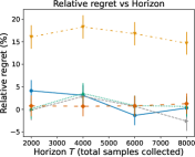
(a) Example 2

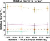
(b) Example 3

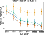
(c) Example 4

Figure 7: The relative regret of different policies across various horizons/budgets for three ATE estimation tasks (error bars denote $95\%$ CIs). We simulate data from synthetic linear causal models and use linear nuisance estimators. In all cases, the online data collection policies outperform the fixed policy as the horizon increases.

Next, we test our methods on the ATE estimation task in Example 4 (also see Fig. 1(c)) with a non-uniform cost structure. The data sources are ${\mathcal{D}}=\left({\mathbb{P}}(U,W,X,Y),{\mathbb{P}}(W,X,Y)\right)$. We set the cost structure $c=[2,1]$, i.e., querying the first data source is twice as costly. We set the model parameters such that the oracle simplex is $\kappa^{*}\approx[0.4,0.6]^{\top}$. We compare our proposed policies to a fixed policy that queries only the first data source with $\kappa_{T}=[1,0]^{\top}$ (see Fig. 7(c)). The fixed policy suffers a constant relative regret of $\approx 35\%$. We observe that the ETC and ETG policies suffer high relative regret at lower budgets. As the budget increases, the ETC and ETG policies converge to zero relative regret.

Appendix I Examples of Online Moment Selection

Example 3 (more details).

Consider the confounder-mediator causal graph (Fig. 1(b)) with a binary treatment $X$, mediator $M$, outcome $Y$, confounder $W$. The target parameter is the causal effect of $X$ on $Y$, i.e., $\beta^{*}={\mathbb{E}}[Y|\text{do}(X=1)]-{\mathbb{E}}[Y|\text{do}(X=0)]$ [Pearl, 2009]. With ${\mathcal{D}}=\{{\mathbb{P}}(W,X,Y),{\mathbb{P}}(X,M,Y)\}$, $\beta^{*}$ can be estimated with the backdoor or the frontdoor criterion [Pearl, 2009, Sec. 3.3]. The moment conditions can be written as

$$g_{t}(\theta)=\begin{bmatrix}s_{t,1}\\ (1-s_{t,1})\end{bmatrix}\odot\begin{bmatrix}\psi_{\text{AIPW}}((W_{t},X_{t},Y_{t});\eta^{\text{(AIPW)}})-\beta\\ \psi_{\text{fd}}((X_{t},M_{t},Y_{t});\eta^{\text{(fd)}})-\beta\end{bmatrix},$$

where $\psi_{\text{AIPW}}$ is defined in Eq. 3 and $\psi_{\text{fd}}$ is the efficient influence function for the frontdoor estimand [Fulcher et al., 2020]:

$$\psi_{\text{fd}}((X_{t},M_{t},Y_{t}); \eta^{\text{(fd)}}_{*})=\frac{p_{1}(M_{t})-p_{0}(M_{t})}{p_{X_{t}}(M_{t})}(Y_{t}-{\mathbb{E}}[Y|X_{t},M_{t}])+$$

$$\begin{aligned} &\frac{X_{t}-(1-X_{t})}{p(X_{t})}\left(\sum_{x\in\{0,1\}}{\mathbb{E}}[Y|x,M_{t}]p(x)-\sum_{x,m}{\mathbb{E}}[Y|x,m]p_{X_{t}}(m)p(x)\right)\\ &+\sum_{m}{\mathbb{E}}[Y|X_{t},m](p_{1}(m)-p_{0}(m)).\end{aligned},$$ (95)

where $p_{x}(m)={\mathbb{P}}(M=m|X=x)$.

Example 5 (Adaptive Neyman allocation).

Consider the setting of a randomized controlled trial with a binary treatment. Let $Y(1)$ and $Y(0)$ denote the potential outcomes [Imbens and Rubin, 2015] for an individual in the treatment and control group, respectively. For each incoming subject, the experimenter must decide whether to assign them to the treatment or the control group [Zhao, 2023, Neyman, 1934]. For this setting, take ${\mathcal{D}}=\left\{{\mathbb{P}}(Y(1)),\,{\mathbb{P}}(Y(0))\right\}$, and

$$g_{t}(\theta)=\begin{bmatrix}s_{t,1}\\ 1-s_{t,1}\end{bmatrix}\odot\begin{bmatrix}Y_{t}(1)-\beta-\alpha\\ Y_{t}(0)-\alpha\end{bmatrix},$$

where $\theta=[\beta,\alpha]^{\top}$ and $f_{\text{tar}}(\theta)=\beta$ is the target parameter (the ATE).

Example 6 (Long-term treatment effects).

In this setting, the aim is to combine experimental data on short-term outcomes and observational data on long-term outcomes to estimate the long-term treatment effect [Athey et al., 2020]. The efficient influence function in Chen and Ritzwoller [2023, Theorem 3.1] can be incorporated into our framework. In the notation of Chen and Ritzwoller [2023], we have

$$g_{t}(\theta)=\begin{bmatrix}s_{t,1}\\ (1-s_{t,1})\end{bmatrix}\odot\begin{bmatrix}\frac{w-(1-w)}{\rho_{w}(s,x)}(y-\mu_{w}(s,x))+\bar{\mu}_{1}(x)-\bar{\mu}_{0}(x)-\beta+\alpha\\ \frac{w-(1-w)}{w\varrho(x)+(1-w)(1-\varrho(x))}(\mu_{w}(s,x)-\bar{\mu}_{w}(x))-\alpha\end{bmatrix},$$

where the target parameter $\beta$ is the long-term ATE.

References

- Abadie et al. [2002] A. Abadie, J. Angrist, and G. Imbens. Instrumental variables estimates of the effect of subsidized training on the quantiles of trainee earnings. Econometrica, 2002.
- Ackerberg et al. [2014] D. Ackerberg, X. Chen, J. Hahn, and Z. Liao. Asymptotic efficiency of semiparametric two-step gmm. Review of Economic Studies, 2014.
- Ailer et al. [2023] E. Ailer, J. Hartford, and N. Kilbertus. Sequential underspecified instrument selection for cause-effect estimation. arXiv preprint arXiv:2302.05684, 2023.
- Angrist and Krueger [1990] J. Angrist and A. B. Krueger. The effect of age at school entry on educational attainment: an application of instrumental variables with moments from two samples, 1990.
- Athey et al. [2020] S. Athey, R. Chetty, and G. Imbens. Combining experimental and observational data to estimate treatment effects on long-term outcomes. arXiv preprint arXiv:2006.09676, 2020.
- Attenberg et al. [2011] J. Attenberg, P. Melville, F. Provost, and M. Saar-Tsechansky. Selective data acquisition for machine learning. Cost-sensitive Machine Learning, 2011.
- Bareinboim and Pearl [2016] E. Bareinboim and J. Pearl. Causal inference and the data-fusion problem. Proceedings of the National Academy of Sciences, 2016.
- Belloni et al. [2017] A. Belloni, V. Chernozhukov, I. Fernandez-Val, and C. Hansen. Program evaluation and causal inference with high-dimensional data. Econometrica, 2017.
- Bhattacharya et al. [2022] R. Bhattacharya, R. Nabi, and I. Shpitser. Semiparametric inference for causal effects in graphical models with hidden variables. Journal of Machine Learning Research, 2022.
- Bickel et al. [1993] P. J. Bickel, C. A. Klaassen, P. J. Bickel, Y. Ritov, J. Klaassen, J. A. Wellner, and Y. Ritov. Efficient and adaptive estimation for semiparametric models. Springer, 1993.
- Billingsley [1995] P. Billingsley. Probability and Measure. Wiley Series in Probability and Statistics. Wiley, 1995.
- Blondin [2007] D. Blondin. Rates of strong uniform consistency for local least squares kernel regression estimators. Statistics & probability letters, 2007.
- Bloom et al. [1997] H. S. Bloom, L. L. Orr, S. H. Bell, G. Cave, F. Doolittle, W. Lin, and J. M. Bos. The benefits and costs of jtpa title ii-a programs: Key findings from the national job training partnership act study. Journal of human resources, 1997.
- Buchinsky et al. [2022] M. Buchinsky, F. Li, and Z. Liao. Estimation and inference of semiparametric models using data from several sources. Journal of Econometrics, 2022.
- Burgess et al. [2016] S. Burgess, F. Dudbridge, and S. G. Thompson. Combining information on multiple instrumental variables in mendelian randomization: comparison of allele score and summarized data methods. Statistics in Medicine, 2016.
- Carneiro et al. [2020] P. Carneiro, S. Lee, and D. Wilhelm. Optimal data collection for randomized control trials. The Econometrics Journal, 2020.
- Chamberlain [1987] G. Chamberlain. Asymptotic efficiency in estimation with conditional moment restrictions. Journal of econometrics, 1987.
- Chandak et al. [2023] Y. Chandak, S. Shankar, V. Syrgkanis, and E. Brunskill. Adaptive instrument design for indirect experiments. In International Conference on Learning Representations, 2023.
- Chen et al. [2022] C. Chen, P. Han, and F. He. Improving main analysis by borrowing information from auxiliary data. Statistics in Medicine, 2022.
- Chen and Ritzwoller [2023] J. Chen and D. M. Ritzwoller. Semiparametric estimation of long-term treatment effects. Journal of Econometrics, 2023.
- Cheng [1984] P. E. Cheng. Strong consistency of nearest neighbor regression function estimators. Journal of Multivariate Analysis, 1984.
- Chernozhukov et al. [2018] V. Chernozhukov, D. Chetverikov, M. Demirer, E. Duflo, C. Hansen, W. Newey, and J. Robins. Double/debiased machine learning for treatment and structural parameters. The Econometrics Journal, 2018.
- Chernozhukov et al. [2022] V. Chernozhukov, J. C. Escanciano, H. Ichimura, W. K. Newey, and J. M. Robins. Locally robust semiparametric estimation. Econometrica, 2022.
- Cohn et al. [1996] D. A. Cohn, Z. Ghahramani, and M. I. Jordan. Active learning with statistical models. Journal of Artificial Intelligence Research, 1996.
- Colnet et al. [2024] B. Colnet, I. Mayer, G. Chen, A. Dieng, R. Li, G. Varoquaux, J.-P. Vert, J. Josse, and S. Yang. Causal inference methods for combining randomized trials and observational studies: a review. Statistical Science, 2024.
- Cook et al. [2023] T. Cook, A. Mishler, and A. Ramdas. Semiparametric efficient inference in adaptive experiments. arXiv preprint arXiv:2311.18274, 2023.
- Csörgö [1968] M. Csörgö. On the strong law of large numbers and the central limit theorem for martingales. Transactions of the American Mathematical Society, 1968.
- Dalal et al. [2024] A. Dalal, P. Blöbaum, S. Kasiviswanathan, and A. Ramdas. Anytime-valid inference for double/debiased machine learning of causal parameters. arXiv preprint arXiv:2408.09598, 2024.
- Donald et al. [2014] S. G. Donald, Y.-C. Hsu, and R. P. Lieli. Testing the unconfoundedness assumption via inverse probability weighted estimators of (l) att. Journal of Business & Economic Statistics, 2014.
- D’Orazio et al. [2006] M. D’Orazio, M. Di Zio, and M. Scanu. Statistical matching: Theory and practice. John Wiley & Sons, 2006.
- Evans et al. [2021] K. Evans, B. Sun, J. Robins, and E. J. T. Tchetgen. Doubly robust regression analysis for data fusion. Statistica Sinica, 2021.
- Farrell et al. [2021] M. H. Farrell, T. Liang, and S. Misra. Deep neural networks for estimation and inference. Econometrica, 2021.
- Francisco-Fernández et al. [2003] M. Francisco-Fernández, J. M. Vilar-Fernández, and J. A. Vilar-Fernández. On the uniform strong consistency of local polynomial regression under dependence conditions. Communications in Statistics-Theory and Methods, 2003.
- Frölich [2007] M. Frölich. Nonparametric iv estimation of local average treatment effects with covariates. Journal of Econometrics, 2007.
- Fulcher et al. [2020] I. R. Fulcher, I. Shpitser, S. Marealle, and E. J. Tchetgen Tchetgen. Robust inference on population indirect causal effects: the generalized front door criterion. Journal of the Royal Statistical Society Series B: Statistical Methodology, 2020.
- Gao et al. [2022] W. Gao, F. Xu, and Z.-H. Zhou. Towards convergence rate analysis of random forests for classification. Artificial Intelligence, 2022.
- Ghassami et al. [2022] A. Ghassami, A. Yang, D. Richardson, I. Shpitser, and E. T. Tchetgen. Combining experimental and observational data for identification and estimation of long-term causal effects. arXiv preprint arXiv:2201.10743, 2022.
- Glynn and Kashin [2018] A. N. Glynn and K. Kashin. Front-door versus back-door adjustment with unmeasured confounding: Bias formulas for front-door and hybrid adjustments with application to a job training program. Journal of the American Statistical Association, 2018.
- Glynn and Kashin [2019] A. N. Glynn and K. Kashin. Replication Data for: Front-Door Versus Back-Door Adjustment With Unmeasured Confounding: Bias Formulas for Front-Door and Hybrid Adjustments With Application to a Job Training Program, 2019. URL https://doi.org/10.7910/DVN/G7NNUL.
- Goodfellow et al. [2016] I. Goodfellow, Y. Bengio, and A. Courville. Deep learning. MIT press, 2016.
- Gorbach et al. [2023] T. Gorbach, X. de Luna, J. Karvanen, and I. Waernbaum. Contrasting identifying assumptions of average causal effects: Robustness and semiparametric efficiency. Journal of Machine Learning Research, 2023.
- Graham et al. [2016] B. S. Graham, C. C. d. X. Pinto, and D. Egel. Efficient estimation of data combination models by the method of auxiliary-to-study tilting (ast). Journal of Business & Economic Statistics, 2016.
- Graham et al. [2024] E. Graham, M. Carone, and A. Rotnitzky. Towards a unified theory for semiparametric data fusion with individual-level data, 2024.
- Guo et al. [2022] W. Guo, S. L. Wang, P. Ding, Y. Wang, and M. Jordan. Multi-source causal inference using control variates under outcome selection bias. Transactions on Machine Learning Research, 2022.
- Gupta et al. [2021a] S. Gupta, Z. C. Lipton, and D. Childers. Efficient online estimation of causal effects by deciding what to observe. In Advances in Neural Information Processing Systems, 2021a.
- Gupta et al. [2021b] S. Gupta, Z. C. Lipton, and D. Childers. Estimating treatment effects with observed confounders and mediators. In Uncertainty in Artificial Intelligence. PMLR, 2021b.
- Györfi et al. [2002] L. Györfi, M. Kohler, A. Krzyzak, H. Walk, et al. A distribution-free theory of nonparametric regression. Springer, 2002.
- Hadad et al. [2021] V. Hadad, D. A. Hirshberg, R. Zhan, S. Wager, and S. Athey. Confidence intervals for policy evaluation in adaptive experiments. The National Academy of Sciences, 2021.
- Hahn et al. [2011] J. Hahn, K. Hirano, and D. Karlan. Adaptive experimental design using the propensity score. Journal of Business & Economic Statistics, 2011.
- Hansen [1982] L. P. Hansen. Large sample properties of generalized method of moments estimators. Econometrica: Journal of the Econometric Society, 1982.
- Häusler and Luschgy [2015] E. Häusler and H. Luschgy. Stable convergence and stable limit theorems. Springer, 2015.
- Henckel et al. [2019] L. Henckel, E. Perković, and M. H. Maathuis. Graphical criteria for efficient total effect estimation via adjustment in causal linear models. arXiv preprint arXiv:1907.02435, 2019.
- Hernán and Robins [2010] M. A. Hernán and J. M. Robins. Causal inference, 2010.
- Howard et al. [2021] S. R. Howard, A. Ramdas, J. McAuliffe, and J. Sekhon. Time-uniform, nonparametric, nonasymptotic confidence sequences. The Annals of Statistics, 2021.
- Hu et al. [2022] W. Hu, R. Wang, W. Li, and W. Miao. Paradoxes and resolutions for semiparametric fusion of individual and summary data. arXiv preprint arXiv:2210.00200, 2022.
- Hu et al. [2018] X. Hu, P. Zhou, P. Li, J. Wang, and X. Wu. A survey on online feature selection with streaming features. Frontiers of Computer Science, 2018.
- Hünermund and Bareinboim [2019] P. Hünermund and E. Bareinboim. Causal inference and data fusion in econometrics. arXiv preprint arXiv:1912.09104, 2019.
- Imbens et al. [2022] G. Imbens, N. Kallus, X. Mao, and Y. Wang. Long-term causal inference under persistent confounding via data combination. arXiv preprint arXiv:2202.07234, 2022.
- Imbens and Rubin [2015] G. W. Imbens and D. B. Rubin. Causal inference in statistics, social, and biomedical sciences. Cambridge University Press, 2015.
- Jeong et al. [2023] D. Jeong, S. Aggarwal, J. Robinson, N. Kumar, A. Spearot, and D. S. Park. Exhaustive or exhausting? evidence on respondent fatigue in long surveys. Journal of Development Economics, 2023.
- Kallus et al. [2024] N. Kallus, X. Mao, and M. Uehara. Localized debiased machine learning: Efficient inference on quantile treatment effects and beyond. Journal of Machine Learning Research, 2024.
- Kato et al. [2020] M. Kato, S. Yasui, and K. McAlinn. The adaptive doubly robust estimator for policy evaluation in adaptive experiments and a paradox concerning logging policy. arXiv preprint arXiv:2010.03792, 2020.
- Kennedy [2016] E. H. Kennedy. Semiparametric theory and empirical processes in causal inference. Statistical causal inferences and their applications in public health research, 2016.
- Kennedy [2022] E. H. Kennedy. Semiparametric doubly robust targeted double machine learning: a review. arXiv preprint arXiv:2203.06469, 2022.
- Kivva et al. [2022] Y. Kivva, E. Mokhtarian, J. Etesami, and N. Kiyavash. Revisiting the general identifiability problem. In Uncertainty in Artificial Intelligence. PMLR, 2022.
- Kohler and Langer [2021] M. Kohler and S. Langer. On the rate of convergence of fully connected deep neural network regression estimates. The Annals of Statistics, 2021.
- Lattimore and Szepesvári [2020] T. Lattimore and C. Szepesvári. Bandit algorithms. Cambridge University Press, 2020.
- Lee and Shpitser [2020] J. J. Lee and I. Shpitser. Identification methods with arbitrary interventional distributions as inputs. arXiv preprint arXiv:2004.01157, 2020.
- Lee et al. [2024] J. J. Lee, A. Ghassami, and I. Shpitser. A general identification algorithm for data fusion problems under systematic selection. In Uncertainty in Artificial Intelligence, 2024.
- Lee and Bareinboim [2020] S. Lee and E. Bareinboim. Causal effect identifiability under partial-observability. In International Conference on Machine Learning. PMLR, 2020.
- Lee and Bareinboim [2021] S. Lee and E. Bareinboim. Causal identification with matrix equations. Advances in Neural Information Processing Systems, 2021.
- Li [2024] H. H. Li. Efficient combination of observational and experimental datasets under general restrictions on outcome mean functions. arXiv preprint arXiv:2406.06941, 2024.
- Li and Owen [2023] H. H. Li and A. B. Owen. Double machine learning and design in batch adaptive experiments. arXiv preprint arXiv:2309.15297, 2023.
- Li and Luedtke [2021] S. Li and A. Luedtke. Efficient estimation under data fusion. arXiv preprint arXiv:2111.14945, 2021.
- Li et al. [2024] W. Li, J. Liu, P. Ding, and Z. Geng. Identification and multiply robust estimation of causal effects via instrumental variables from an auxiliary heterogeneous population. arXiv preprint arXiv:2407.18166, 2024.
- Li et al. [2021] X. Li, W. Miao, F. Lu, and X.-H. Zhou. Improving efficiency of inference in clinical trials with external control data. Biometrics, 2021.
- Li et al. [2022] X. Li, Y. Li, Q. Cui, L. Li, and J. Zhou. Robust direct learning for causal data fusion. arXiv preprint arXiv:2211.00249, 2022.
- Li and Oliva [2021] Y. Li and J. Oliva. Active feature acquisition with generative surrogate models. In International Conference on Machine Learning. PMLR, 2021.
- Liero [1989] H. Liero. Strong uniform consistency of nonparametric regression function estimates. Probability theory and related fields, 1989.
- Lin and Chen [2014] H.-W. Lin and Y.-H. Chen. Adjustment for missing confounders in studies based on observational databases: 2-stage calibration combining propensity scores from primary and validation data. American journal of epidemiology, 2014.
- Lin et al. [2023] L. Lin, K. Khamaru, and M. J. Wainwright. Semi-parametric inference based on adaptively collected data. arXiv preprint arXiv:2303.02534, 2023.
- Lin et al. [2024] X. Lin, J. M. Tarp, and R. J. Evans. Data fusion for efficiency gain in ate estimation: A practical review with simulations. arXiv preprint arXiv:2407.01186, 2024.
- Morrison et al. [2024] T. Morrison, M. Nguyen, M. Baiocchi, and A. B. Owen. Constrained design of a binary instrument in a partially linear model. arXiv preprint arXiv:2406.05592, 2024.
- Newey [1990] W. K. Newey. Semiparametric efficiency bounds. Journal of applied econometrics, 1990.
- Newey and McFadden [1994] W. K. Newey and D. McFadden. Large sample estimation and hypothesis testing. Handbook of econometrics, 1994.
- Neyman [1934] J. Neyman. On the two different aspects of the representative method: The method of stratified sampling and the method of purposive selection. Journal of the Royal Statistical Society, 1934.
- Neyman [1959] J. Neyman. Optimal asymptotic tests of composite hypotheses. Probability and statsitics, 1959.
- Pearl [2009] J. Pearl. Causality. Cambridge university press, 2009.
- Rahimi and Recht [2007] A. Rahimi and B. Recht. Random features for large-scale kernel machines. Advances in Neural Information Processing Systems, 2007.
- Rakhlin et al. [2015] A. Rakhlin, K. Sridharan, and A. Tewari. Sequential complexities and uniform martingale laws of large numbers. Probability theory and related fields, 2015.
- Ramdas et al. [2023] A. Ramdas, P. Grünwald, V. Vovk, and G. Shafer. Game-theoretic statistics and safe anytime-valid inference. Statistical Science, 2023.
- Ramsahai [2012] R. R. Ramsahai. Supplementary variables for causal estimation. Causality: Statistical perspectives and applications, 2012.
- Ridder and Moffitt [2007] G. Ridder and R. Moffitt. The econometrics of data combination. Handbook of econometrics, 2007.
- Rotnitzky and Smucler [2020] A. Rotnitzky and E. Smucler. Efficient adjustment sets for population average causal treatment effect estimation in graphical models. Journal of Machine Learning Research, 2020.
- Rotnitzky et al. [2021] A. Rotnitzky, E. Smucler, and J. M. Robins. Characterization of parameters with a mixed bias property. Biometrika, 2021.
- Saar-Tsechansky et al. [2009] M. Saar-Tsechansky, P. Melville, and F. Provost. Active feature-value acquisition. Management Science, 2009.
- Settles [2009] B. Settles. Active learning literature survey. In University of Wisconsin-Madison Department of Computer Sciences, 2009.
- Shi et al. [2023] X. Shi, Z. Pan, and W. Miao. Data integration in causal inference. Wiley Interdisciplinary Reviews: Computational Statistics, 2023.
- Shim et al. [2018] H. Shim, S. J. Hwang, and E. Yang. Joint active feature acquisition and classification with variable-size set encoding. Advances in Neural Information Processing Systems, 2018.
- Shinoda and Hoshino [2022] K. Shinoda and T. Hoshino. Estimation of local average treatment effect by data combination. In AAAI Conference on Artificial Intelligence, 2022.
- Shuai et al. [2023] K. Shuai, S. Luo, W. Li, and Y. He. Identifying causal effects using instrumental variables from the auxiliary population. arXiv preprint arXiv:2309.02087, 2023.
- Stürmer et al. [2005] T. Stürmer, S. Schneeweiss, J. Avorn, and R. J. Glynn. Adjusting effect estimates for unmeasured confounding with validation data using propensity score calibration. American journal of epidemiology, 2005.
- Sun and Miao [2022] B. Sun and W. Miao. On semiparametric instrumental variable estimation of average treatment effects through data fusion. Statistica Sinica, 2022.
- Tauchen [1985] G. Tauchen. Diagnostic testing and evaluation of maximum likelihood models. Journal of Econometrics, 1985.
- Tikka et al. [2019] S. Tikka, A. Hyttinen, and J. Karvanen. Causal effect identification from multiple incomplete data sources: A general search-based approach. arXiv preprint arXiv:1902.01073, 2019.
- Tsiatis [2006] A. A. Tsiatis. Semiparametric theory and missing data. Springer, 2006.
- Van der Vaart [2000] A. W. Van der Vaart. Asymptotic Statistics. Cambridge University Press, 2000.
- Wainwright [2019] M. J. Wainwright. High-dimensional statistics: A non-asymptotic viewpoint, volume 48. Cambridge university press, 2019.
- Walk [2010] H. Walk. Strong laws of large numbers and nonparametric estimation. In Recent Developments in Applied Probability and Statistics: Dedicated to the Memory of Jürgen Lehn. Springer, 2010.
- Waudby-Smith et al. [2021] I. Waudby-Smith, D. Arbour, R. Sinha, E. H. Kennedy, and A. Ramdas. Time-uniform central limit theory, asymptotic confidence sequences, and anytime-valid causal inference. arXiv preprint arXiv:2103.06476, 2021.
- Witte et al. [2020] J. Witte, L. Henckel, M. H. Maathuis, and V. Didelez. On efficient adjustment in causal graphs. Journal of Machine Learning Research, 2020.
- Wu et al. [2023] A. Wu, K. Kuang, R. Xiong, M. Zhu, Y. Liu, B. Li, F. Liu, Z. Wang, and F. Wu. Learning instrumental variable from data fusion for treatment effect estimation. In AAAI Conference on Artificial Intelligence, 2023.
- Wu et al. [2020] Y. Wu, X. Wang, and N. Balakrishnan. On the consistency of the p–c estimator in a nonparametric regression model. Statistical Papers, 2020.
- Yang and Ding [2019] S. Yang and P. Ding. Combining multiple observational data sources to estimate causal effects. Journal of the American Statistical Association, 2019.
- Zhao [2023] J. Zhao. Adaptive neyman allocation. arXiv preprint arXiv:2309.08808, 2023.
- Zhao et al. [2019] Q. Zhao, J. Wang, W. Spiller, J. Bowden, and D. S. Small. Two-sample instrumental variable analyses using heterogeneous samples. Statistical Science, 2019.
- Zhao et al. [2024] Y. Zhao, K.-S. Jun, T. Fiez, and L. Jain. Adaptive experimentation when you can’t experiment. arXiv preprint arXiv:2406.10738, 2024.
- Zhao and Yao [2012] Z. Zhao and W. Yao. Sequential design for nonparametric inference. Canadian Journal of Statistics, 2012.
- Zrnic and Candès [2024] T. Zrnic and E. J. Candès. Active statistical inference. arXiv preprint arXiv:2403.03208, 2024.