Nonlinear Evolution of unstable Charged de Sitter Black Holes with Hyperboloidal Formalism
Abstract
Based on the hyperboloidal framework, we research the dynamical process of charged de Sitter black holes scattered by a charged scalar field. From the linear perturbation analysis, with the coupling strength within a critical interval, the charged scalar field with a superradiance frequency can induce the instability of the system. To reveal the real-time dynamics of such an instability, the nonlinear numerical simulation is implemented. The results show that the scalar field grows exponentially in the early stages and drastically extracts the charge from the black hole due to the superradiance, analogous to the charged black hole in a closed system. Differently, after saturation, the scalar field can not coexist with the central black hole stably and dissipates beyond the cosmological horizon slowly, leaving behind a bald black hole.
I Introduction
Superradiance, a radiation amplification process, is of great significance in numerous fields of physics, particularly in relativity and astrophysics [1]. In General Relativity, black hole (BH) superradiance results from the interaction between BHs with angular momentum or charge and their surrounding environments, leading to the extraction of energy, charge, and angular momentum from BHs. If there is a confinement mechanism, the scattering field will be incapable of escaping the trap and will grow over time at the expense of the BH’s energy, known as the superradiant instability or “BH bomb” [2].
In the linear regime, the superradiant instabilities of various BH-bomb systems have been studied extensively, such as BHs enclosed in a reflecting mirror [3, 4, 5, 6, 7, 8], BHs in anti-de Sitter (AdS) backgrounds [9, 10, 11, 12, 13, 8, 14, 15] and spinning BHs with massive bosonic fields in asymptotically flat spacetimes [16, 17, 18, 19, 20, 4, 21, 22]. In the above models, artificial reflection boundary conditions, gravitational potential of spacetime, and self-interaction of matter fields provide confinement mechanisms respectively. Intriguingly, for gravitational systems that lack explicit confinement mechanisms, such as charged BHs scattered by charged scalar fields in asymptotically de Sitter (dS) spacetime, a novel instability of superradiant nature is discovered, where the superradiance is a necessary but not sufficient condition [23, 24, 25, 26, 27, 28, 29, 30, 31]. Such an instability has also been found in charged BHs surrounded by anisotropic fluids [32].
To deal with saturation and the final state of superradiant instabilities, however, is beyond the scope of the linear perturbation theory and necessitates a fully nonlinear approach. Complicated by challenges such as very small growth rates, significant disparities in scale between the BH and superradiant fields, and inherently (3+1)-dimensional nonlinear equations [33, 34], only a few nonlinear evolutions of the superradiant instability have been successfully simulated in rotating BH bombs [35, 36, 37, 38] and charged BH bombs [39, 40, 41, 42]. The latter, compared with its rotating counterpart, is easier to numerically evolve to a stationary final state by reason that the charged superradiant instability has a larger growth rate and can even be explored in spherical symmetry [6]. It was shown that a hairy BH with a harmonically oscillating scalar field condensate is the endpoint of charged BH bombs induced by an artificial mirror [43, 39, 40] or the AdS boundary [41, 44].
A natural question that arises is what is the final state of a charged BH bomb in dS spacetime? On the one hand, the results of linear perturbation theory show that such a system suffers from dynamical instability, indicating that an arbitrarily small perturbation can induce drastic changes in gravitational configuration, thereby driving the system to undergo a dynamical transition. On the other hand, a no charged scalar hair theorem for static dS BHs has been established [45], which precludes the possibility of the formation of a hairy BH. Such a contradiction motivates the implementation of nonlinear dynamics simulation. So far, a few studies have performed nonlinear evolutions of scalar field perturbations in Reissner-Nordström (RN)-dS spacetime for strong cosmic censorship [46, 47].
To address the question, we study the nonlinear evolution of charged dS BHs scattered by a charged scalar field, based on the hyperboloidal framework, in which quasi-normal boundary conditions are inherently satisfied since no characteristics are directed to the computational domain [48, 49, 50]. Hyperboloidal foliations intersect with the future cosmological horizon (respectively null infinity), where the total mass (respectively the Bondi mass) or charge of the asymptotically dS (respectively flat) spacetime can be evaluated straightforwardly [51]. At the superradiant growth stage, a rapid loss of total mass and charge of the asymptotically dS spacetime, such an unconfined system, is observed, and the initial growth rates predicted by the linear analysis are also verified. In contrast to the charged BH bombs discussed in the previous paragraph, the scalar field cannot coexist with the central BH after saturation. Instead, the scalar field dissipates beyond the cosmological horizon at a gradual rate, thereby reinforcing the assertion that the final state is still a bald BH with less charge [45].
The paper is organized as follows: In Section II, we introduce the hyperboloidal formalism we used. In Section III, we review the linear stability analysis of charged scalar fields for RN-dS BHs. In Section IV we show our numerical results of non-linear evolutions for the instability with superradiant nature and discuss impacts of some free parameters. Finally, in Section V we sum up our concluding remarks.
In this paper, we use the unit .
II Hyperboloidal Formalism
In this section, we describe our hyperboloidal formalism, in which boundary conditions, field equations and foliations of spacetime are revealed.
II.1 Hyperboloidal coordinates
In order to achieve the spherically symmetric dynamics we are concerned with here, inspired by the hyperboloidal compactification technique [48, 49, 50], we adopt a hyperboloidal coordinates with Bondi-Sachs-like gauge choices [52, 53]: 111There are some other types of hyperboloidal evolution formalism with different gauge conditions, e.g. ADM-like formulation on constant mean curvature surfaces [54, 55, 51] and the Generalized BSSN or Z4 formulations [56, 57, 58].
| (1) | ||||
where we take the area radius as a coordinate, is the line element of unit sphere , and are metric functions dependent on . The boost function determines the locations of physical boundaries, i.e. the apparent horizon and cosmological horizon , which are located at respectively. Additionally, the quasi-normal boundary conditions for a BH, such an open system, that the purely ingoing wave at the BH event horizon and outgoing wave at the cosmological horizon are inherently satisfied in the hyperboloidal coordinates (1).
To show this, we compute the outgoing/ingoing radial null characteristic speeds by solving for the eikonal equation
| (2) |
Setting , we obtain the outgoing radial null characteristic speed
| (3) |
and the ingoing one
| (4) |
Note that at the apparent horizon vanishes and is positive, and at the cosmological horizon vanishes and is negative, which is precisely what the quasi-normal boundary conditions require.
II.2 Field equations
As a concrete example, we consider the model where a charged scalar field is minimally coupled to the Einstein-Maxwell system in asymptotically dS spacetime with the action 222Note that and here are dimensionless. The dimensionful physical fields are
| (5) |
| (6) |
where represents the Ricci scalar, represents the positive cosmological constant, represents the field strength with the electromagnetic potential, is the gauge covariant derivative with denoting the gauge coupling constant, and represents the mass of the scalar field.
Varying the action (5), three equations of motion are obtained
| (7) |
| (8) |
| (9) |
where the energy-momentum tensors are given by
| (10) |
| (11) |
and the Noether current is given by
| (12) |
The model is invariant under a local gauge transformation , where is a regular real function of spacetime coordinates.
Using the hyperboloidal coordinates (1), taking the gauge potential and introducing auxiliary variables
| (13) |
| (14) |
where dot and prime denote the derivative with respect to the temporal coordinate and the radial coordinate respectively, one can reduce the field equations to a system of equations with a simple nested structure:
Einstein equations
| (15) |
| (16) | ||||
| (17) | ||||
Maxwell equations
| (18) |
| (19) |
and the scalar field equation
| (20) |
For the specific implementation of dynamical evolution, we use the so-called constrained evolution scheme. The evolutionary equations for all the dynamical variables are comprised of eqs.(14)-(16), (18) and (20), by which we can calculate the temporal derivatives of all the dynamical variables.
Eqs.(13), (17) and (19) serve as the constraint equations. We obtain by solving eq.(13) and eqs.(17, 19) are used to check the validity of our numerics (See Appendix.C for more details).
We exclude from the dynamical variables because the evolutionary equation of (See 40) is redundant, which can be derived from eqs.(15), (16) and (17) using the Bianchi identity. Instead, we use eq.(15), the component of momentum constraint, to solve . The constraint equation (17) will be preserved during the evolution, provided that it is satisfied on the initial time slice. See Appendix.A.1 for more details.
II.3 Foliations of RN-dS
In order to simulate the dynamical process of scattering a charged BH by a scalar field, we first need to obtain the metric functions of the RN-dS BH solution in the hyperboloidal coordinates (1).
Solving the Einstein-Maxwell equations with , one can find the RN-dS BH solution is described by and
| (21) |
where and represent the total mass and charge of the BH respectively. Here are a few things to note.
First, the constant parameter cannot be arbitrarily set and it depends on and . The value of needs to be chosen such that is a continuous real function decreasing monotonically from 1, at the cosmological horizon , to , at the apparent horizon . There exists a zero between and , and by solving the set of equations
| (22) |
one can obtain 333In this paper, we fix the initial BH mass such that evaluated in (23) is close to 1.
| (23) | ||||
| (24) |
where .
Second, the function takes the positive square root of eq.(21) when and the negative square root when .
Third, the transformation from the Schwarzschild coordinates
| (25) |
to the hyperboloidal coordinates (1) can be obtained by the height function technique [48, 49]:
| (26) |
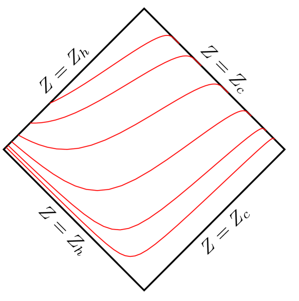
with , where is called the height function. It can be seen that our foliations penetrate both the outer horizon and the cosmological horizon (See Fig.1).
III Linear Stability Analysis
Before showing the nonlinear dynamical evolution, we would like to review the linear stability analysis of RN-dS BHs using the hyperboloidal formalism. 444The results obtained in the hyperboloidal formalism were checked with [24, 27].
The linearized scalar perturbation equation on the RN-dS background is given by eqs.(14) and (20), where the background electromagnetic potential is chosen as . We follow the scheme of numerically calculating the quasi-normal modes with linearized dynamic evolution [59, 60], which can results in a generalized eigenvalue problem [61] (see also [62] for its application in inhomogeneous backgrounds and [63] for that in backgrounds even without time-translation symmetry).
By expanding and with harmonic time dependence , the temporal derivatives are replaced by . Meanwhile, the coordinate is discretized with Chebyshev-Gauss-Lobatto grid points and then the radial derivatives can be replaced by the corresponding differentiation matrix [64, 65]. Thus, the quasi-normal frequencies can be obtained by solving the resulting generalized eigenvalue equation 555One has to be careful about false modes caused by the discretization, which can be examined by varying the grid number.
| (27) |
with
| (28) |
| (29) |
where represent the identity matrix and the null matrix respectively, and represent diagonal matrices of the grid points and the grid function respectively. As mentioned in Sec.II.1, the quasi-normal boundary conditions are inherently satisfied in the hyperboloidal coordinates.
As already found in [23, 24, 27], the occurrence of instability in this system mainly depends on the charge coupling , the scalar mass and the cosmological constant . It was shown that for small enough (less than a critical mass ), there exists an interval where the unstable superradiant modes could occur 666We only consider the case due to the symmetry of eq.(27) ..
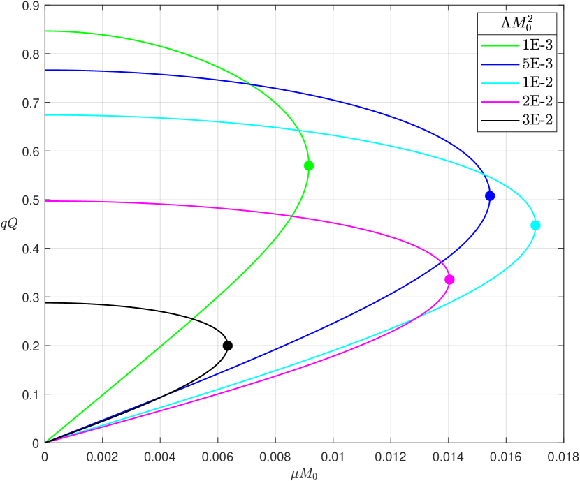
As shown in Fig.2, while decreases from to zero, increases, whereas decreases to zero (Also see Fig.5 in [27]). In addition, the critical mass increases first and then decreases with the increment of . While reaches beyond a critical value , no instability is observed.
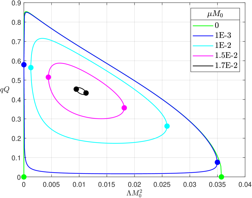
For the case of a massless scalar field, unstable modes appear for arbitrarily small [24, 27]. However, we find that the situation with massive scalar fields is completely different. As shown in Fig.3, when , there exists a lower bound , below which no instability can be observed. As the scalar mass increases to a critical value, the region shrinks until it disappears.
IV Nonlinear Dynamical Evolution
In this section, we present our numerical evolutions of the Einstein-Maxwell-Scalar- (EMS) system derived in the Sec.II.2. In Sec.IV.1 we briefly describe our numerical setup. The initial data for RN-dS BHs with charged scalar fields are constructed in Sec.IV.2. In Sec.IV.3, we will describe a general picture for the full nonlinear evolution of the instability driven by superradiance. Finally in Sec.IV.4, we discuss the effects of four free parameters on the dynamics of the system: the scalar mass , the cosmological constant , the charge coupling 777We only show the result for , for results for other value of are qualitatively the same. and the scalar field amplitude .
IV.1 Numerical setup
To efficiently perform longtime evolutions, we employ explicit fourth-fifth order Runge-Kutta method [66, 67] along the time direction and Chebyshev pseudo-spectral method (see e.g.[64, 65]) in the radial direction.
The simulation takes place within a larger domain than the region between the apparent horizon and cosmological horizon , which ensures that the physical evolution in can be fully determined by initial data. Note that and at , thereby , which means the radius of cosmological horizon does not decrease during evolution. Thus, needs to be small enough to prevent the cosmological horizon from expanding beyond during evolution. We empirically set and in our simulations.
As discussed in Sec.II.1, we do not need to impose physical boundary conditions888A boundary condition for the gauge field is still needed. We set in our simulations., even if our actual simulation domain .
IV.2 Initial data
As we have five first-order temporal derivative equations (14)-(16), (18), (20) and two constraints eqs.(17), (19), the initial value can be completely determined by three of the five dynamical variables . In our case, we freely choose the initial data of and solve via the two constraints.
We impose the following initial scalar perturbation on the seed RN-dS BH:
| (30) |
| (31) |
where is the amplitude, is the centre, and is the width of initial Gaussian wave packet. For such a form of perturbation, on the one hand, the total mass of the spacetime, evaluated by the rescaled Misner-Sharp mass (See 53) at the cosmological horizon , increases with the amplitude . On the other hand, the total charge of the perturbed system remains unchanged, indicating the initial scalar perturbation is neutral. Such a result can be derived from the constraint eq.(19), where is a constant associated with the BH initial charge (See 51). We have also used other functional forms of perturbation, such as linear functions. All the numerical results are qualitatively the same.
The existence of the scalar perturbation will deform the RN-dS metric functions and . We choose to satisfy , which gives
| (32) |
This choice makes the constraint equation (17) equivalent to , that is,
| (33) |
Integrating eq.(33) numerically to solve may require a little trick, see Appendix.A.2 for more details.
IV.3 General picture
In order to give a general picture of the evolution of the EMS system, we show the characteristic behaviors of some key physical quantities including the scalar field value on the apparent horizon, the scalar field energy and charge , as well as the BH charge , the BH Mass , irreducible mass , and the total charge and total mass of the spacetime (See Appendix.B for detailed calculations).
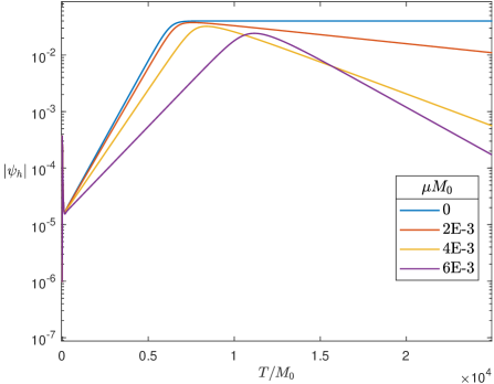
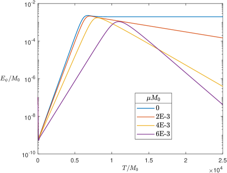
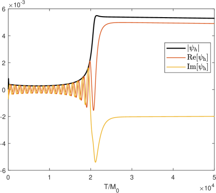
The time evolution of exhibited in the left panel of Fig.4 shows two distinct stages. During the first stage, the so-called superradiant growth stage, the scalar field grows exponentially, as expected by the linear stability analysis (see Table.1). During the second stage, the relaxation stage, the scalar field reaches saturation and then decays slowly (exponentially as well). Since the spacetime background changes also slowly at the relaxation stage, we can adopt adiabatic approximation to analyze the decay rates of the relaxing scalar fields at a linear level [68] (see also Table.1). The similar behavior of the corresponding evolution of the scalar field energy is exhibited in the right panel of Fig.4.
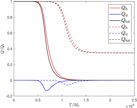
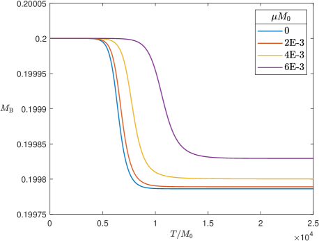
As depicted in the left panel of Fig.5, at the superradiant growth stage, a large portion of the scalar field with the opposite sign to the BH charge is absorbed into the apparent horizon, leading to a sharp reduction in the BH charge. Meanwhile, most of the scalar field with the same sign as the BH charge is repelled beyond the cosmological horizon, resulting in a greater decrease in the system’s total charge and a negative net charge of the scalar field. Additionally, the BH experiences a slight reduction in mass during the superradiant growth stage (See the right panel of Fig.5).
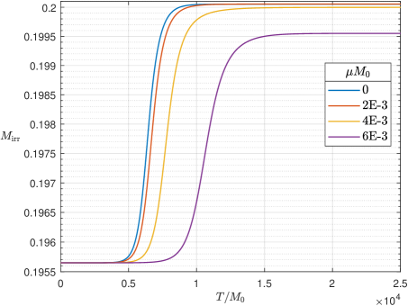
As shown in Fig.6, the irreducible mass increases rapidly at the superradiant growth stage, then remains nearly a constant at the relaxation stage. Such a result that the irreducible mass does not decrease throughout the evolution abides by the area law. Finally, shown in the right panel of Fig.6, the total mass of spacetime does not increase throughout the evolution, as a result of charged scalar radiation.
| 0 | 0.00126749 | 0.00126817 | 0 | 0.8466 | 1.33E-7 | -4.9E-8 | 8.4E-8 | 99.89% | 0 | 0 |
| 2E-4 | 0.00126690 | 0.00126758 | 0.0098 | 0.8466 | 1.62E-7 | -5.8E-8 | 1.04E-7 | 99.89% | -7.36E-7 | -7.15E-7 |
| 2E-3 | 0.00120829 | 0.00120865 | 0.0984 | 0.8390 | 0.0024 | -8.3E-5 | 0.0023 | 99.89% | -7.36E-5 | -7.16E-6 |
| 4E-3 | 0.00102937 | 0.00102935 | 0.1975 | 0.8153 | 0.1232 | -1.1E-5 | 0.1232 | 99.90% | -2.61E-4 | -2.53E-4 |
| 6E-3 | 0.00072810 | 0.00072797 | 0.3004 | 0.7728 | 0.3470 | -2.3E-6 | 0.3470 | 99.91% | -3.89E-4 | -3.79E-4 |
IV.4 Detailed description
In the previous subsection, our results have shown that the scattering process of charged scalar fields can extract charge and mass from the central RN-dS BHs through superradiance. Since the occurrence of this instability in this system is strongly linked to the charge coupling, we focus on the effects of the four free parameters on the amount of charge extracted from the BH in this subsection.
Predictably, denotes the saturation point of the instability. We find that in the case of the massless scalar field, where , the BH charge decays exponentially. However, for massive scalar fields (), the amount of charge extracted from the BH is associated with the difference . More specifically, the bigger the difference , the more charge of the BH is extracted. In the following, we run simulations with different parameters to verify this claim.
IV.4.1 Impact of the scalar mass and cosmological constant
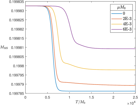
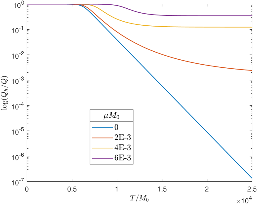
As discussed in Sec.III, the lower bound of the charge coupling interval governing the instability of the system, denoted as , is subject to influence from the scalar mass and the cosmological constant . Thus, we adjust and to vary while fixing the initial charge coupling .
As shown in Fig.7 and Table.1, the more massive the scalar field is, the less charge the BH loses. It is noteworthy that in the case of the massless scalar field, the charge of the BH decays exponentially, which implies the final BH could be almost neutral.
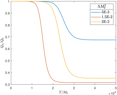
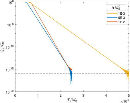
Results with different are shown in Fig.8 and Table.2. In the context of the massive scalar field, the RN-dS BH with the moderate , thereby smaller , loses more charge. However, in the case of the massless scalar field, always vanishes for . Consequently, for different , the numerical values of the BH charge all decrease exponentially to , the nominal round-off level for the double precision employed.
| 0.5E-2 | 0.2458 | 0.7046 | 67.47% | 1.4E-7 | 67.47% | 99.88% |
| 1.5E-2 | 0.1742 | 0.5471 | 31.54% | 1.6E-11 | 31.54% | 99.64% |
| 2.5E-2 | 0.2177 | 0.3231 | 35.21% | 5.7E-8 | 35.21% | 99.58% |
Thus, we can conclude that when the parameters except and are fixed, the smaller is, the more complete the charge extraction will be.
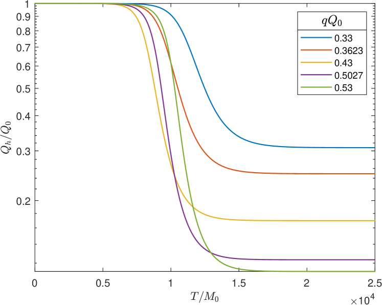
IV.4.2 Impact of the charge coupling
To investigate the impact of the charge coupling, we keep the and to fix , and then vary the initial . As shown in Fig.9, when is fixed, the larger initial charge coupling (not larger than ), the more charge is extracted from the BH.
Thus, taking the result of the previous subsubsection into consideration, we conclude that the amount of charge extracted from the BH is associated with the difference .
IV.4.3 Impact of the scalar field amplitude
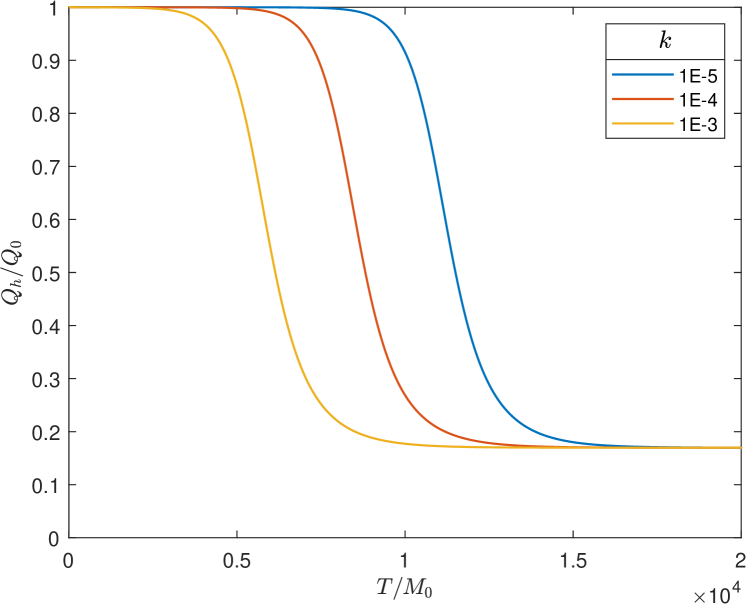
One might also think that the amount of charge extracted from the BH could be affected by the scalar field amplitude . However, we find that the scalar field amplitude hardly affects the amount of charge extracted from the BH, and that a larger could advance the start time of the superradiant growth stage (See Fig.10).
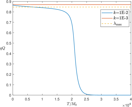
More intriguingly, a significant perturbation with an initial charge coupling beyond can also trigger this instability (See Fig.11). In the case of the right panel of Fig.11, the superradiant mode is stable at the early stage. Nevertheless, a larger initial amplitude enhance the early charge extraction. Thus, an initial charge coupling beyond can enter the unstable interval at some point, where the superradiant mode becomes unstable.
V Conclusions
In the present work, we study the dynamical process of charged dS BHs scattered by a charged scalar field with the hyperboloidal formalism.
For studying gravitational systems in asymptotically dS spacetime, the hyperboloidal formalism has many advantages. On the one hand, the structure of field equations is simple. On the other hand, since the foliations penetrate both the apparent horizon and the cosmological horizon, the physical boundary conditions are inherently satisfied, which greatly simplifies the work of stability analysis and dynamical simulation of the system. In addition, the hyperboloidal formalism we employed is also well-suited for gravitational systems in asymptotically flat spacetime without recourse to the conformal transformation.
The linear stability analysis of the RN-dS BH scattered by a charged scalar field is reviewed within the hyperboloidal framework. Our results agree well with those in the previous literature. Moreover, we find that black holes of intermediate size, relative to the radius of the cosmological horizon, are prone to instabilities induced by massive scalar fields.
The nonlinear numerical simulations are implemented to reveal the real-time dynamical process of such an instability. Our main result is that the scalar field grows exponentially at the superradiant growth stage, leading to a substantial loss of the charge of the black hole. The scalar field then slowly dissipates beyond the cosmological horizon, causing the total charge of the spacetime to decrease and eventually leaving behind a bald black hole. The massless scalar field relaxes to a constant value at late-time and the charge of the BH decreases exponentially, which implies the final BH could be almost neutral. However, for massive scalar fields, the amount of charge extracted from the BH is associated with the difference . In addition, significant perturbations with an initial charge coupling beyond can also trigger such an instability.
As is known to all, in addition to charged BHs, rotating BHs can also trigger superradiance. Therefore, a further meaningful study is the superradiance process of Kerr BHs in asymptotically dS spacetime scattered by a scalar field [69, 70, 71, 72, 73]. Such a process will induce the release of gravitational waves, which is of great astronomical observation significance. Furthermore, there are indications that critical phenomena between the more/less charged BH transition (analogous to the gravitational collapse [74, 75, 76, 77, 78, 79, 80, 81] or the bald/scalarized BH transition [82, 83, 84, 85, 86]) may exist in the superradiance process of the EMS system, which we reserve for further study.
Acknowledgements.
We would like to thank Ulrich Sperhake and Carlos A.R. Herdeiro for their helpful discussions. Zhen-Tao He would like to thank Jia Du for his help with Mathematica, Zhuan Ning and Yu-Kun Yan for discussions about the generalized eigenvalue method, and Meng Gao for discussions about Newton-Raphson iteration algorithm. This work is partly supported by the National Key Research and Development Program of China (Grant No.2021YFC2203001). This work is supported in part by the National Natural Science Foundation of China under Grants No. 12035016, No. 12075026, No. 12275350, No. 12375048, No. 12375058 and. No. 12361141825.Appendix A Calculation details
A.1 The structure of Einstein equations
The structure of the Einstein field equations in hyperboloidal formalism can be clarified with the help of the ADM 3+1 formulation.
Define the future directed unit normal covector of the -constant hypersurface
| (34) |
and the induced metric on
| (35) |
Eq.(15) is equivalent to the component of momentum constraint
| (36) | ||||
where and . On the third and fourth lines, we rewrite eq.(15) and call it for convenience.
One can obtain that eq.(17), called , is exactly
| (37) | ||||
where the Hamiltonian constraint is defined as
| (38) |
The evolutionary equation (16) of , called , is exactly
| (39) | ||||
The last Einstein equation including temporal derivative of is
| (40) | ||||
Using the Bianchi identity of the Einstein tensor and the covariant conservation of the energy-momentum tensor , we can get
| (41) |
A.2 The construction of the initial data
Integrating eq.(33), we have
| (45) |
where is the right hand side of eq.(33) and is an undetermined integration constant dependent on the lower limit of integral.
Similar to Sec.II.3, we need to find the zero of to the square root of eq.(45). To do this we substitute into eq.(45) and its derivative with respect to , and get
| (46) |
| (47) |
One can solve numerically via eq.(46), so that
| (48) |
which could ensure . Note that can be set freely.
To set the simulation domain , we need to solve the initial positions of and , which can be obtained by substituting and into eq.(48) respectively. That is, both the initial and are the roots of the equation .
Appendix B Physical quantities
We monitor the evolution of several physical quantities during our simulation: the scalar field energy , scalar field charge , black hole charge the irreducible mass and the rescaled Misner-Sharp mass .
The scalar field energy is calculated as follows:
| (49) | ||||
Note that the scalar field energy density is nonnegative, satisfying the weak energy condition.
The scalar field charge is associated with the Nother charge for the conserved current :
| (50) | ||||
The black hole charge is evaluated by
| (51) |
where represents the Hodge star operation. The total charge of the spacetime, in the hyperboloidal coordinates, can be evaluated at the future cosmological horizon straightforwardly,
The irreducible mass is , where represents the apparent horizon area.
The mass of the BH can be calculated as
| (52) |
This formula is valid for the initial and final state of evolutions where the spacetime region near the apparent horizon is almost static.
The rescaled Misner-Sharp mass is defined as [87]
| (53) |
and the total mass of the spacetime is evaluated at the future cosmological horizon .
Appendix C Numerical error and convergence
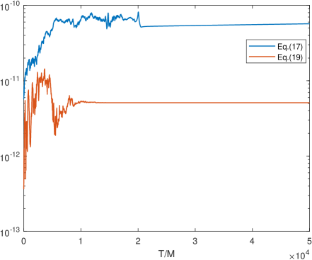
As mentioned in II.2, eq.(17) and (19) are used as the constraint equations to check the validity of our numerics. We have checked that all of them remain satisfied throughout our evolution.
To be specific, we calculate the relative variation for eq.(17), where is defined in 37 and represents the sum of the absolute value of each term in eq.(17), i.e.
| (54) |
But the calculation of the relative variation is not applicable to eq.(19), because each term in eq.(19) is very close to zero in the early and late stages of evolution. We straightly calculate the absolute value of right hand side for eq.(19). We show the variation of the maximal constraint violations along the direction with time in Fig.12.
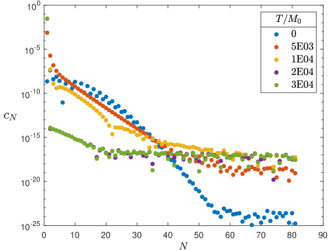
We have also checked the spectral convergence of our numerical simulation by examining spectral coefficients for each dynamical variable. We demonstrate such a spectral convergence for in Fig.12, where one can see the exponential convergence.
References
- Brito et al. [2020] R. Brito, V. Cardoso, and P. Pani, Superradiance – the 2020 edition, Lecture Notes in Physics 971 (2020) 10.1007/978-3-030-46622-0 (2020), arXiv:1501.06570 [gr-qc] .
- Press and Teukolsky [1972] W. H. Press and S. A. Teukolsky, Floating Orbits, Superradiant Scattering and the Black-hole Bomb, Nature 238, 211 (1972).
- Cardoso et al. [2004] V. Cardoso, O. J. C. Dias, J. P. S. Lemos, and S. Yoshida, Black-hole bomb and superradiant instabilities, Phys. Rev. D 70, 044039 (2004).
- Dolan [2013] S. R. Dolan, Superradiant instabilities of rotating black holes in the time domain, Phys. Rev. D 87, 124026 (2013), arXiv:1212.1477 [gr-qc] .
- Degollado and Herdeiro [2014] J. C. Degollado and C. A. R. Herdeiro, Time evolution of superradiant instabilities for charged black holes in a cavity, Phys. Rev. D 89, 063005 (2014).
- Degollado et al. [2013] J. C. Degollado, C. A. R. Herdeiro, and H. F. Rúnarsson, Rapid growth of superradiant instabilities for charged black holes in a cavity, Phys. Rev. D 88, 063003 (2013).
- Hod [2013] S. Hod, Analytic treatment of the charged black-hole-mirror bomb in the highly explosive regime, Phys. Rev. D 88, 064055 (2013).
- Ferreira and Herdeiro [2018] H. R. C. Ferreira and C. A. R. Herdeiro, Superradiant instabilities in the kerr-mirror and kerr-ads black holes with robin boundary conditions, Phys. Rev. D 97, 084003 (2018), arXiv:1712.03398 [gr-qc] .
- Cardoso and Dias [2004] V. Cardoso and O. J. C. Dias, Small kerr–anti-de sitter black holes are unstable, Phys. Rev. D 70, 084011 (2004), arXiv:hep-th/0405006 .
- Uchikata et al. [2009] N. Uchikata, S. Yoshida, and T. Futamase, Scalar perturbations of kerr-ads black holes, Phys. Rev. D 80, 084020 (2009).
- Rosa [2010] J. G. Rosa, The Extremal black hole bomb, JHEP 06, 015, arXiv:0912.1780 [hep-th] .
- Cardoso et al. [2014] V. Cardoso, O. J. C. Dias, G. S. Hartnett, L. Lehner, and J. E. Santos, Holographic thermalization, quasinormal modes and superradiance in Kerr-AdS, JHEP 04, 183, arXiv:1312.5323 [hep-th] .
- Wang and Herdeiro [2016] M. Wang and C. Herdeiro, Maxwell perturbations on kerr–anti–de sitter black holes: Quasinormal modes, superradiant instabilities, and vector clouds, Phys. Rev. D 93, 064066 (2016), arXiv:1512.02262 [gr-qc] .
- Uchikata and Yoshida [2011] N. Uchikata and S. Yoshida, Quasinormal modes of a massless charged scalar field on a small reissner-nordström-anti-de sitter black hole, Phys. Rev. D 83, 064020 (2011), arXiv:1109.6737 [gr-qc] .
- González et al. [2017] P. A. González, E. Papantonopoulos, J. Saavedra, and Y. Vásquez, Superradiant instability of near extremal and extremal four-dimensional charged hairy black holes in anti–de sitter spacetime, Phys. Rev. D 95, 064046 (2017), arXiv:1702.00439 [gr-qc] .
- Furuhashi and Nambu [2004] H. Furuhashi and Y. Nambu, Instability of massive scalar fields in kerr-newman spacetime, Prog.Theor.Phys. 112 (2004) 983-995 112, 983 (2004), arXiv:gr-qc/0402037 [gr-qc] .
- Cardoso and Yoshida [2005] V. Cardoso and S. Yoshida, Superradiant instabilities of rotating black branes and strings, JHEP 07, 009, arXiv:hep-th/0502206 .
- Strafuss and Khanna [2005] M. J. Strafuss and G. Khanna, Massive scalar field instability in kerr spacetime, Phys. Rev. D 71, 024034 (2005), arXiv:gr-qc/0412023 .
- Dolan [2007] S. R. Dolan, Instability of the massive klein-gordon field on the kerr spacetime, Phys. Rev. D 76, 084001 (2007).
- Witek et al. [2013] H. Witek, V. Cardoso, A. Ishibashi, and U. Sperhake, Superradiant instabilities in astrophysical systems, Phys. Rev. D 87, 043513 (2013).
- Cardoso et al. [2018a] V. Cardoso, O. J. C. Dias, G. S. Hartnett, M. Middleton, P. Pani, and J. E. Santos, Constraining the mass of dark photons and axion-like particles through black-hole superradiance, JCAP 03, 043, arXiv:1801.01420 [gr-qc] .
- Dolan [2018] S. R. Dolan, Instability of the proca field on kerr spacetime, Phys. Rev. D 98, 104006 (2018), arXiv:1806.01604 [gr-qc] .
- Zhu et al. [2014] Z. Zhu, S.-J. Zhang, C. E. Pellicer, B. Wang, and E. Abdalla, Stability of reissner-nordström black hole in de sitter background under charged scalar perturbation, Phys. Rev. D 90, 044042 (2014), arXiv:1405.4931 [hep-th] .
- Konoplya and Zhidenko [2014] R. A. Konoplya and A. Zhidenko, Charged scalar field instability between the event and cosmological horizons, Phys. Rev. D 90, 064048 (2014), arXiv:1406.0019 [hep-th] .
- Cardoso et al. [2018b] V. Cardoso, J. a. L. Costa, K. Destounis, P. Hintz, and A. Jansen, Strong cosmic censorship in charged black-hole spacetimes: Still subtle, Phys. Rev. D 98, 104007 (2018b), arXiv:1808.03631 [gr-qc] .
- Mo et al. [2018] Y. Mo, Y. Tian, B. Wang, H. Zhang, and Z. Zhong, Strong cosmic censorship for the massless charged scalar field in the reissner-nordstrom–de sitter spacetime, Phys. Rev. D 98, 124025 (2018), arXiv:1808.03635 [gr-qc] .
- Destounis [2019] K. Destounis, Superradiant instability of charged scalar fields in higher-dimensional reissner-nordström-de sitter black holes, Phys. Rev. D 100, 044054 (2019), arXiv:1908.06117 [gr-qc] .
- Dias et al. [2019] O. J. C. Dias, H. S. Reall, and J. E. Santos, Strong cosmic censorship for charged de Sitter black holes with a charged scalar field, Class. Quant. Grav. 36, 045005 (2019), arXiv:1808.04832 [gr-qc] .
- Liu et al. [2021] P. Liu, C. Niu, and C.-Y. Zhang, Instability of regularized 4D charged Einstein-Gauss-Bonnet de-Sitter black holes, Chin. Phys. C 45, 025104 (2021), arXiv:2004.10620 [gr-qc] .
- González et al. [2022] P. A. González, E. Papantonopoulos, J. Saavedra, and Y. Vásquez, Quasinormal modes for massive charged scalar fields in reissner-nordström ds black holes: anomalous decay rate, JHEP 06, 150, arXiv:2204.01570 [gr-qc] .
- Mascher et al. [2022] G. Mascher, K. Destounis, and K. D. Kokkotas, Charged black holes in de sitter space: Superradiant amplification of charged scalar waves and resonant hyperradiation, Phys. Rev. D 105, 084052 (2022), arXiv:2204.05335 [gr-qc] .
- Cuadros-Melgar et al. [2021] B. Cuadros-Melgar, R. D. B. Fontana, and J. de Oliveira, Superradiance and instabilities in black holes surrounded by anisotropic fluids, Phys. Rev. D 104, 104039 (2021), arXiv:2108.04864 [gr-qc] .
- Lehner [2001] L. Lehner, Numerical relativity: A review, Class.Quant.Grav.18:R25-R86,2001 18, R25 (2001), arXiv:gr-qc/0106072 [gr-qc] .
- Choptuik et al. [2015] M. W. Choptuik, L. Lehner, and F. Pretorius, Probing strong field gravity through numerical simulations, ArXiv e-prints 10.48550/ARXIV.1502.06853 (2015), arXiv:1502.06853 [gr-qc] .
- East and Pretorius [2017] W. E. East and F. Pretorius, Superradiant instability and backreaction of massive vector fields around kerr black holes, Phys. Rev. Lett. 119, 041101 (2017), arXiv:1704.04791 [gr-qc] .
- East [2018] W. E. East, Massive boson superradiant instability of black holes: Nonlinear growth, saturation, and gravitational radiation, Phys. Rev. Lett. 121, 131104 (2018), arXiv:1807.00043 [gr-qc] .
- Chesler and Lowe [2019] P. M. Chesler and D. A. Lowe, Nonlinear evolution of the superradiant instability, Phys. Rev. Lett. 122, 181101 (2019).
- Chesler [2022] P. M. Chesler, Hairy black resonators and the superradiant instability, Phys. Rev. D 105, 024026 (2022), arXiv:2109.06901 [gr-qc] .
- Sanchis-Gual et al. [2016a] N. Sanchis-Gual, J. C. Degollado, P. J. Montero, J. A. Font, and C. Herdeiro, Explosion and final state of an unstable reissner-nordström black hole, Phys. Rev. Lett. 116, 141101 (2016a).
- Sanchis-Gual et al. [2016b] N. Sanchis-Gual, J. C. Degollado, C. Herdeiro, J. A. Font, and P. J. Montero, Dynamical formation of a reissner-nordström black hole with scalar hair in a cavity, Phys. Rev. D 94, 044061 (2016b), arXiv:1607.06304 [gr-qc] .
- Bosch et al. [2016] P. Bosch, S. R. Green, and L. Lehner, Nonlinear evolution and final fate of charged anti–de sitter black hole superradiant instability, Phys. Rev. Lett. 116, 141102 (2016), arXiv:1601.01384 [gr-qc] .
- Zhang et al. [2024] C.-Y. Zhang, Q. Chen, Y. Liu, Y. Tian, B. Wang, and H. Zhang, Nonlinear self-interaction induced black hole bomb, Phys. Rev. D 110, L041505 (2024), arXiv:2309.05045 [gr-qc] .
- Dolan et al. [2015] S. R. Dolan, S. Ponglertsakul, and E. Winstanley, Stability of black holes in einstein-charged scalar field theory in a cavity, Phys. Rev. D 92, 124047 (2015), arXiv:1507.02156 [gr-qc] .
- Dias and Masachs [2017] O. J. C. Dias and R. Masachs, Hairy black holes and the endpoint of ads4 charged superradiance, JHEP 1702 (2017) 128 2017, 10.1007/jhep02(2017)128 (2017), arXiv:1610.03496 [hep-th] .
- An and Li [2023] Y.-P. An and L. Li, Static de-Sitter black holes abhor charged scalar hair, Eur. Phys. J. C 83, 569 (2023), arXiv:2301.06312 [gr-qc] .
- Luna et al. [2019] R. Luna, M. Zilhão, V. Cardoso, J. a. L. Costa, and J. Natário, Strong cosmic censorship: The nonlinear story, Phys. Rev. D 99, 064014 (2019).
- Zhang and Zhong [2019] H. Zhang and Z. Zhong, Strong cosmic censorship in de sitter space: As strong as ever, (2019), arXiv:1910.01610 [hep-th] .
- Zenginoglu [2008] A. Zenginoglu, Hyperboloidal foliations and scri-fixing, Class. Quant. Grav. 25, 145002 (2008), arXiv:0712.4333 [gr-qc] .
- Zenginoğlu [2011] A. i. e. i. f. Zenginoğlu, A geometric framework for black hole perturbations, Phys. Rev. D 83, 127502 (2011).
- Ripley et al. [2021] J. L. Ripley, N. Loutrel, E. Giorgi, and F. Pretorius, Numerical computation of second-order vacuum perturbations of kerr black holes, Phys. Rev. D 103, 104018 (2021), 2010.00162 .
- Baake and Rinne [2016] O. Baake and O. Rinne, Superradiance of a charged scalar field coupled to the einstein-maxwell equations, Phys. Rev. D 94, 124016 (2016), arXiv:1610.08352 [gr-qc] .
- Bondi et al. [1962] H. Bondi, M. G. J. van der Burg, and A. W. K. Metzner, Gravitational waves in general relativity. 7. Waves from axisymmetric isolated systems, Proc. Roy. Soc. Lond. A 269, 21 (1962).
- Sachs [1962] R. K. Sachs, Gravitational waves in general relativity. 8. Waves in asymptotically flat space-times, Proc. Roy. Soc. Lond. A 270, 103 (1962).
- Rinne [2010] O. Rinne, An axisymmetric evolution code for the einstein equations on hyperboloidal slices, Class.Quant.Grav.27:035014,2010 27, 035014 (2010), arXiv:0910.0139 [gr-qc] .
- Rinne and Moncrief [2013] O. Rinne and V. Moncrief, Hyperboloidal Einstein-matter evolution and tails for scalar and Yang-Mills fields, Class. Quant. Grav. 30, 095009 (2013), arXiv:1301.6174 [gr-qc] .
- Vañó Viñuales and Husa [2015] A. Vañó Viñuales and S. Husa, Unconstrained hyperboloidal evolution of black holes in spherical symmetry with GBSSN and Z4c, J. Phys. Conf. Ser. 600, 012061 (2015), arXiv:1412.4801 [gr-qc] .
- Vañó-Viñuales et al. [2015] A. Vañó-Viñuales, S. Husa, and D. Hilditch, Spherical symmetry as a test case for unconstrained hyperboloidal evolution, Class. Quantum Grav. 32 (2015) 175010 32, 175010 (2015), arXiv:1412.3827 [gr-qc] .
- Vañó Viñuales and Husa [2017] A. Vañó Viñuales and S. Husa, Free hyperboloidal evolution in spherical symmetry, in 14th Marcel Grossmann Meeting on Recent Developments in Theoretical and Experimental General Relativity, Astrophysics, and Relativistic Field Theories, Vol. 2 (2017) pp. 2025–2030, arXiv:1601.04079 [gr-qc] .
- Li et al. [2015] R. Li, Y. Tian, H. Zhang, and J. Zhao, Time domain analysis of superradiant instability for the charged stringy black hole-mirror system, Phys. Lett. B 750, 520 (2015), arXiv:1506.04267 [hep-th] .
- Du et al. [2015] Y. Du, C. Niu, Y. Tian, and H. Zhang, Holographic thermal relaxation in superfluid turbulence, JHEP 1512 (12), 018, arXiv:1412.8417 [hep-th] .
- Dias et al. [2010] O. J. C. Dias, P. Figueras, R. Monteiro, H. S. Reall, and J. E. Santos, An instability of higher-dimensional rotating black holes, JHEP 1005:076,2010 2010, 10.1007/jhep05(2010)076 (2010), arXiv:1001.4527 [hep-th] .
- Guo et al. [2020] M. Guo, E. Keski-Vakkuri, H. Liu, Y. Tian, and H. Zhang, Dynamical phase transition from nonequilibrium dynamics of dark solitons, Phys. Rev. Lett. 124, 031601 (2020), arXiv:1810.11424 [hep-th] .
- Yang et al. [2023] P. Yang, M. Baggioli, Z. Cai, Y. Tian, and H. Zhang, Holographic dissipative spacetime supersolids, Phys. Rev. Lett. 131, 221601 (2023), arXiv:2304.02534 [hep-th] .
- Trefethen [2000] L. N. Trefethen, Spectral Methods in MatLab (Society for Industrial and Applied Mathematics, USA, 2000).
- Press et al. [2007] W. H. Press, S. A. Teukolsky, W. T. Vetterling, and B. P. Flannery, Numerical Recipes 3rd Edition: The Art of Scientific Computing, 3rd ed. (Cambridge University Press, USA, 2007).
- Dormand and Prince [1980] J. Dormand and P. Prince, A family of embedded runge-kutta formulae, Journal of Computational and Applied Mathematics 6, 19 (1980).
- Shampine and Reichelt [1997] L. F. Shampine and M. W. Reichelt, The matlab ode suite, SIAM Journal on Scientific Computing 18, 1 (1997), https://doi.org/10.1137/S1064827594276424 .
- Brito et al. [2015] R. Brito, V. Cardoso, and P. Pani, Black holes as particle detectors: evolution of superradiant instabilities, Class. Quant. Grav. 32, 134001 (2015), arXiv:1411.0686 [gr-qc] .
- Tachizawa and ichi Maeda [1993] T. Tachizawa and K. ichi Maeda, Superradiance in the kerr-de sitter space-time, Physics Letters A 172, 325 (1993).
- Anninos and Anous [2010] D. Anninos and T. Anous, A de Sitter Hoedown, JHEP 08, 131, arXiv:1002.1717 [hep-th] .
- Georgescu et al. [2014] V. Georgescu, C. Gérard, and D. Häfner, Asymptotic completeness for superradiant klein-gordon equations and applications to the de sitter kerr metric 10.48550/ARXIV.1405.5304 (2014), arXiv:1405.5304 [math.AP] .
- Zhang et al. [2014] C.-Y. Zhang, S.-J. Zhang, and B. Wang, Superradiant instability of Kerr-de Sitter black holes in scalar-tensor theory, JHEP 08, 011, arXiv:1405.3811 [hep-th] .
- Bhattacharya [2018] S. Bhattacharya, Kerr-de sitter spacetime, penrose process, and the generalized area theorem, Phys. Rev. D 97, 084049 (2018), arXiv:1710.00997 [gr-qc] .
- Choptuik [1993] M. W. Choptuik, Universality and scaling in gravitational collapse of a massless scalar field, Phys. Rev. Lett. 70, 9 (1993).
- Abrahams and Evans [1993] A. M. Abrahams and C. R. Evans, Critical behavior and scaling in vacuum axisymmetric gravitational collapse, Phys. Rev. Lett. 70, 2980 (1993).
- Evans and Coleman [1994] C. R. Evans and J. S. Coleman, Critical phenomena and self-similarity in the gravitational collapse of radiation fluid, Phys. Rev. Lett. 72, 1782 (1994).
- Gundlach [1995] C. Gundlach, Choptuik spacetime as an eigenvalue problem, Phys. Rev. Lett. 75, 3214 (1995).
- Koike et al. [1995] T. Koike, T. Hara, and S. Adachi, Critical behavior in gravitational collapse of radiation fluid: A renormalization group (linear perturbation) analysis, Phys. Rev. Lett. 74, 5170 (1995).
- Garfinkle and Duncan [1998] D. Garfinkle and G. C. Duncan, Scaling of curvature in subcritical gravitational collapse, Phys. Rev. D 58, 064024 (1998).
- Choptuik et al. [2004] M. W. Choptuik, E. W. Hirschmann, S. L. Liebling, and F. Pretorius, Critical collapse of a complex scalar field with angular momentum, Phys. Rev. Lett. 93, 131101 (2004).
- Gundlach and Martin-Garcia [2007] C. Gundlach and J. M. Martin-Garcia, Critical phenomena in gravitational collapse, LivingRev.Rel.10:5,2007 10, 10.12942/lrr-2007-5 (2007), arXiv:0711.4620 [gr-qc] .
- Zhang et al. [2022a] C.-Y. Zhang, Q. Chen, Y. Liu, W.-K. Luo, Y. Tian, and B. Wang, Critical phenomena in dynamical scalarization of charged black holes, Phys. Rev. Lett. 128, 161105 (2022a), arXiv:2112.07455 [gr-qc] .
- Zhang et al. [2022b] C.-Y. Zhang, Q. Chen, Y. Liu, W.-K. Luo, Y. Tian, and B. Wang, Dynamical transitions in scalarization and descalarization through black hole accretion, Phys. Rev. D 106, L061501 (2022b), arXiv:2204.09260 [gr-qc] .
- Jiang et al. [2023] J.-Y. Jiang, Q. Chen, Y. Liu, Y. Tian, W. Xiong, C.-Y. Zhang, and B. Wang, Type i critical dynamical scalarization and descalarization in einstein-maxwell-scalar theory, Sci. China Phys. Mech. Astron. 67, 220411 (2023), arXiv:2306.10371 [gr-qc] .
- Chen et al. [2023] Q. Chen, Z. Ning, Y. Tian, B. Wang, and C.-Y. Zhang, Nonlinear dynamics of hot, cold, and bald einstein-maxwell-scalar black holes in ads spacetime, Phys. Rev. D 108, 084016 (2023), arXiv:2307.03060 [gr-qc] .
- Liu et al. [2023] Y. Liu, C.-Y. Zhang, Q. Chen, Z. Cao, Y. Tian, and B. Wang, Critical scalarization and descalarization of black holes in a generalized scalar-tensor theory, Sci. China Phys. Mech. Astron. 66, 100412 (2023), arXiv:2208.07548 [gr-qc] .
- Maeda [2012] H. Maeda, Exact dynamical ads black holes and wormholes with a klein-gordon field, Phys. Rev. D 86, 044016 (2012).