Frequency locking: a distinctive feature of the coherent population trapping
and the stationarity effect

Abstract

We study the case where phase modulation of the harmonic signal is used to obtain the error signal for the frequency stabilization to a reference atomic transition. High-frequency modulation, or analog of the Pound-Drever-Hall regime, is considered. We demonstrate that for coherent population trapping, the maximal error-signal slope retains at a certain level with growth in the modulation frequency, while for other types of resonances it drops steadily. The investigation of the low-frequency modulation regime reveals the stationarity effect. We show that in this case, the maximal steepness of the error signal does not depend on the modulation frequency and is reached at a fixed value of the frequency deviation.

I Introduction

The basic idea behind the microwave [1, 2] or optical [3] frequency standard is to compare the local oscillator frequency with that of a reference atomic transition. Among the former, the most widespread and used are clocks based on microwave transition between magneto-insensitive sublevels (in the linear approximation) in the ground state $\textbf{nS}_{1/2}$ of alkali-metal atoms. The classic example is the rubidium atomic frequency standards, which utilize the double radio-optical resonance [4]. The pumping light source of ⁸⁷Rb atoms enclosed in a glass-blowing cell is a discharge lamp, and the reference transition is interrogated by an rf field from the microwave cavity. Designed and commercialized in the $1960$s, they are now the workhorse of the telecommunications industry and satellites of global navigation systems [4, 5].

The all-optical effect of coherent population trapping (CPT), discovered in the $1970$s [6, 7, 8, 9, 10], has led to the development of chip-scale atomic clocks in the $2000$s and their commercialization in the early $2010$s [11]. The pumping light produced by the current-modulated vertical-cavity surface-emitting diode laser [12], the microfabricated glass cell with alkali-metal atoms [13] and no need to use the microwave cavity [14] are the reasons why the CPT-based atomic clocks became unrivaled in size, weight, and power consumption among the frequency standards [15]. This feature determined the use of such devices in unmanned vehicles, underwater sensor systems, small satellites, military applications, etc. [16, 17].

The long-term frequency stability of rubidium and chip-scale atomic clocks is hard to improve. Nowadays, there are emerging compact optical clocks since the stabilized laser frequency can be moved down to the consumer range by means of frequency combs based on high-quality microresonators [18]. Such a frequency standards are also based on glass cells with alkali-metal atoms. Two notable examples are clocks utilizing the two-photon transition in ⁸⁷Rb atoms [19] and those that use sub-Doppler resonance in the alkali-metal atoms D₁ line induced by counter-propagating bichromatic laser waves [20]. Both approaches are promising to provide the frequency stability at the level of $10^{-13}$ at $1$ s (ADEV).

For all the clocks mentioned above, the reference resonance is an even function of the detuning, and therefore it cannot be directly used to stabilize the local oscillator frequency. One common approach to obtain the error signal with a dispersive shape is to use the lock-in technique based on the phase modulation of the interrogating field’s frequency, $s(t)=\cos{\left(\omega_{0}t+m\sin{\omega_{m}t}\right)}$. Here $m$ is the phase modulation index, $\omega_{m}$ is the modulation frequency. As a result the light absorption oscillates at frequencies $n\omega_{m}$, $n>0$, among which the first harmonic $n=1$ is most often used. Amplitude of the corresponding oscillations can be represented as the sum of the in-phase ($\propto\cos{\omega_{m}t}$) and quadrature ($\propto\sin{\omega_{m}t}$) signals. They can be obtained from the absorption signal by the synchronous detection technique. In a general case a mixture like $A_{\text{In-ph}}\cos{\alpha}-A_{\text{Q}}\sin{\alpha}$, where $A_{\text{In-ph}}$ and $A_{\text{Q}}$ are amplitudes of the signals, should be used to maximize slope of the error signal, where $\alpha$ is the synchronous detection phase.

It is convenient to treat $s(t)$ in the spectral interpretation using the Jacobi-Anger expansion, $e^{-im\sin{\omega_{m}}t}=\sum^{\infty}_{k=-\infty}J_{k}(m)e^{-ik\omega_{m}t}$, where $J_{k}(\cdot)$ is the Bessel function of the first kind of the index $k$. In this case one can demonstrate, that non-oscillating part of the light absorption is a group of Lorentzians spaced by $\omega_{m}$, i.e., it acquires a multipeak structure. As we have recently shown for the case of the CPT resonance [21], this feature leads to the frequency pulling of the error signal under an asymmetry. However, this effect can be suppressed in a high-frequency modulation, or analog of the Pound-Drever-Hall regime [22], where the peaks are well resolved. The question remains in the degree of the error-signal slope reduction compared to the maximal possible value, which is achieved when the peaks are not resolved.

In this work we show that the maximal slope of the error signal steadily drops when the modulation frequency is increased beyond the width of the optical transition in two-level system and the width of double-radio optical resonance. The CPT effect, on the contrary, turns out to be unique: the steepness retains at a certain level with $\omega_{m}$ growth in the high-frequency regime. We also demonstrate that for all systems of levels mentioned above there is the stationarity effect: the maximal error-signal slope is constant when $\omega_{m}$ is much smaller than the interrogated transition width.

We begin from the CPT effect and consider the $\Lambda$-system of levels: the excited-state level is $|e\rangle$, ground-state levels $|a\rangle$ and $|b\rangle$ are spaced by the frequency interval $\omega_{g}$; see Fig. 1a. The following bichromatic optical field

$$\mathcal{E}(t)=-\dfrac{\mathcal{E}_{0}}{2}\left\{e^{-i\left[(\omega_{0}-\Omega)t-\varphi(t)\right]}-e^{-i\left[(\omega_{0}+\Omega)t+\varphi(t)\right]}\right\}+\text{c.\,c.},$$ (1)

couples $|a\rangle$ and $|b\rangle$ with $|e\rangle$. The low-frequency component induces transitions only between levels $|a\rangle$ and $|e\rangle$, while the high-frequency component works on the opposite shoulder of the $\Lambda$-scheme. The frequency $\omega_{0}$ is taken to be equal to half-sum of the optical transitions and $\omega_{0}\gg\omega_{g}$. The dipole moments of both transitions are assumed to be equal and real. The term $\varphi(t)=m\sin{\omega_{m}}t$ accounts for the modulation required for producing in-phase and quadrature signals. The frequency $\Omega$ is close to $\omega_{g}/2$, and the difference gives the two-photon detuning $\delta=2\Omega-\omega_{g}$.

The initial equations for the density matrix elements can be treated by adiabatically eliminating the excited state, using the rotating wave approximation, and assuming the low saturation regime. Here we cite the simplified equations obtained in our previous work [21]:

$$\rho_{ee}=2\dfrac{V^{2}}{\gamma\Gamma}\left\{1-2\text{Re}\left[e^{2i\varphi(t)}\bar{\rho}_{ab}(t)\right]\right\},$$ (2)

$$\left(i\frac{\partial}{\partial t}+\delta+i\tilde{\Gamma}_{g}\right)\bar{\rho}_{ab}=i\dfrac{V^{2}}{\Gamma}e^{-2i\varphi(t)},$$ (3)

where $\rho_{ee}$ is the excited-state population and $\bar{\rho}_{ab}$ is the slow amplitude of the non-diagonal element of the density matrix between levels of $\Lambda$-system’s ground state, $\bar{\rho}_{ab}=\rho_{ab}e^{-2i\Omega t}$. $V=d\mathcal{E}_{0}/2\hbar$ is the Rabi frequency, $\gamma$ is the spontaneous decay rate of the excited-state population, $\Gamma$ is the relaxation rate of the optical coherences, which describes homogeneous broadening of the optical line. The relaxation parameter $\tilde{\Gamma}_{g}=\Gamma_{g}+2V^{2}/\Gamma$ accounts for the power broadening of the CPT resonance by the optical field. The hierarchy of parameters is the following:

$$\delta,\,\tilde{\Gamma}_{g},\,\omega_{m},\,V^{2}/\Gamma\ll\gamma\ll\Gamma\ll\Omega,\,\omega_{g}\ll\omega_{0}.$$ (4)

Figure 1: Systems of levels under consideration.

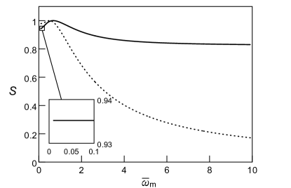
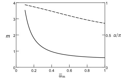
Figure 2: (a) Solid curve: dependence of the maximal error-signal slope on the ratio of the modulation frequency $\omega_{m}$ to the ground-state relaxation rate $\tilde{\Gamma}_{g}$ for the CPT resonance. The maximum value is normalized to be unity. The inset demonstrates the low-frequency region, the curve is plotted via Eq. (7). Dashed curve: the same but for the two-level system, where $\bar{\omega}_{m}=\omega_{m}/(\gamma/2)$. (b) The corresponding dependence of the modulation index $m$ (solid curve) and the synchronous detection phase $\alpha$ (in units of $\pi$, dashed curve) providing the maximal error-signal slope for the CPT resonance.

By using the Jacobi-Anger expansion and the Fourier one for $\rho_{ee}$ and $\bar{\rho}_{ab}$ over $\omega_{m}$, we get the following expression determining response of the system at the frequency $\omega_{m}$:

$$\begin{gathered}A^{\text{CPT}}_{1}=-4\dfrac{V^{2}}{\gamma\Gamma}\text{Re}\bigg{\{}i\sum^{\infty}_{k=-\infty}J_{k}(2m)\left[J_{k-1}(2m)e^{-i\omega_{m}t}\right.\\ \left.+J_{k+1}(2m)e^{i\omega_{m}t}\right]\dfrac{V^{2}/\Gamma}{\delta+k\omega_{m}+i\tilde{\Gamma}_{g}}\bigg{\}}.\end{gathered}$$ (5)

The amplitudes of in-phase and quadrature signals in the experiment are obtained by the synchronous detection technique:

$$\langle\rho_{ee}\cos{(\omega_{m}t+\alpha)}\rangle,$$ (6)

where $\langle\dots\rangle$ means averaging over period of the frequency $\omega_{m}$. In the case of numerical results, presented in Figs. 2, 2, we have investigated the range $\alpha\in(0,\,\pi)$. The absolute value of steepness was obtained by linearization of the in-phase and quadrature signals amplitudes over $\delta$. The maximal slope is reached at $\omega_{m}/\tilde{\Gamma}_{g}\simeq 0.764$, $m\simeq 0.652$ and $\alpha\simeq 3\pi/4$, which is in accordance with work [23].

As we will see further, in comparison to the case of the two-level system and the double radio-optical resonance, the expression (5) does not contain the term like $1/(\omega_{m}+i\tilde{\Gamma}_{g})$ before the sum. This results in the constant level of the error-signal steepness at $\omega_{m}\gg\tilde{\Gamma}_{g}$; see Fig. 2. In the high-frequency modulation regime, the slope is given by the central dispersive curve of the quadrature signal, which is proportional to the product $J_{0}(2m)J_{1}(2m)$ and does not depend on $\omega_{m}$; see [21]. The maximizing value of $m$ is $\simeq 0.54$. Dependencies, presented in Figs. 2, 2, were numerically obtained by accounting terms from $k=-100$ to $k=100$ in the sums.

The maximizing value of the modulation index $m$ grows when the frequency $\omega_{m}$ is decreased beyond $\tilde{\Gamma}_{g}$; see Fig. 2. This feature stems from the structure of the in-phase signal:

$$\begin{gathered}A^{\text{CPT}}_{\text{In-ph}}\propto\sum^{\infty}_{k=-\infty}J_{k}(2m)\dfrac{J_{k-1}(2m)+J_{k+1}(2m)}{(\bar{\delta}+k\bar{\omega}_{m})^{2}+1}\\ \equiv-4\bar{\delta}\dfrac{\bar{\omega}_{m}}{m}\sum^{\infty}_{k=1}\dfrac{\left[kJ_{k}(2m)\right]^{2}}{\left[(\bar{\delta}+k\bar{\omega}_{m})^{2}+1\right]\left[(\bar{\delta}-k\bar{\omega}_{m})^{2}+1\right]}\\ \underset{\bar{\delta}\ll 1}{\simeq}-4\bar{\delta}\dfrac{\bar{\omega}_{m}}{m}\sum^{\infty}_{k=1}\left[\dfrac{kJ_{k}(2m)}{\left(k\bar{\omega}_{m}\right)^{2}+1}\right]^{2},\end{gathered}$$ (7)

where $\bar{\delta}=\delta/\tilde{\Gamma}_{g}$, $\bar{\omega}_{m}=\omega_{m}/\tilde{\Gamma}_{g}$. The first line of this formula demonstrates that dispersive shape of the signal stems from pairs of Lorentzians symmetrically located with respect to the point $\bar{\delta}=0$ but having opposite signs. The slope of each pair is maximized when they are shifted by $\simeq 0.58\tilde{\Gamma}_{g}$ from the point $\bar{\delta}=0$. Therefore, with decrease in $\bar{\omega}_{m}$, the slope is determined by pairs of Lorentzian given by greater $|k|$; see the expression in the third line of Eq. 7. In its turn, for $k\gg 1$, the corresponding Bessel functions are maximized at $m\propto k$. Therefore, the value of $m$ maximizing the steepness grows as $1/\bar{\omega}_{m}$ under decreasing of $\bar{\omega}_{m}$ at $\bar{\omega}_{m}\ll 1$. Fig. 2 demonstrates that the corresponding dependence of $m$ on $\bar{\omega}_{m}$ is the hyperbola. The numerical calculation reveals that the maximal error-signal slope provided by the in-phase signal is constant at $\bar{\omega}_{m}\ll 1$. In the time representation this means that the frequency deviation does not change.

We continue with the two-level system considering the case of the optical transition between the single ground level $|g\rangle$ and the excited state $|e\rangle$ (see Fig. 1b) induced by the phase-modulated field:

$$\mathcal{E}(t)=\mathcal{E}_{0}e^{-i\left[\omega_{L}t+\varphi(t)\right]}/2+\text{c.\,c.}$$ (8)

The equations for the density matrix elements under the rotating wave approximation and the low saturation regime are the following:

$$i\dfrac{\partial}{\partial t}\rho_{ee}=V\left(e^{-i\varphi(t)}\rho_{ge}-\text{c.\,c.}\right)-i\gamma\rho_{ee},$$ (9)

$$\left(i\dfrac{\partial}{\partial t}+\Delta_{L}+i\gamma/2\right)\rho_{eg}=Ve^{-i\varphi(t)}.$$ (10)

Here $V=d\mathcal{E}_{0}/2\hbar$ is the Rabi frequency, $\gamma$ is the natural width of the excited state, and $\Delta_{L}=\omega_{L}-\omega_{0}$ is the frequency detuning. The spacing between the excited and ground states is $\omega_{0}$. This equations are valid for $\gamma,\Delta_{L},V\ll\omega_{0}$.

The amplitudes of the in-phase and quadrature signals are determined by the real and imaginary parts of the following expression:

$$\begin{gathered}A^{\text{Two-level}}_{1}=\dfrac{V^{2}}{\omega_{m}+i\gamma}\\ \sum^{\infty}_{k=-\infty}J_{k}(m)\left[\dfrac{J_{k+1}(m)}{\Delta_{L}+k\omega_{m}-i\gamma/2}-\dfrac{J_{k-1}(m)}{\Delta_{L}+k\omega_{m}+i\gamma/2}\right].\end{gathered}$$ (11)

As far as the term before the sum has $\omega_{m}$ in the denominator, the maximal steepness of the error signal falls in the high-frequency modulation regime. We demonstrate this explicitly at strong inequality $\omega_{m}\gg\gamma/2$, where the error-signal steepness is determined by the central dispersive curve, which amplitude reads as

$$A_{\text{C}}=2J_{0}(m)J_{1}(m)\dfrac{S}{\bar{\omega}_{m}}\dfrac{\bar{\Delta}_{L}}{\bar{\Delta}^{2}_{L}+1},$$ (12)

where $\bar{\Delta}_{L}=\Delta_{L}/(\gamma/2)$, $\bar{\omega}_{m}=\omega_{m}/(\gamma/2)$, $S=\left[V/(\gamma/2)\right]^{2}$. Eq. (12) shows linear decrease of $A_{\text{C}}$ with $\bar{\omega}_{m}$.

The stationarity effect also takes place. We get for $\bar{\omega}_{m}\ll 1$, $\bar{\Delta}_{L}\ll 1$ that the biggest term of the in-phase signal amplitude is given by

$$A^{\text{Two-level}}_{\text{In-ph}}=-4\bar{\Delta}_{L}S\dfrac{\bar{\omega}_{m}}{m}\sum^{\infty}_{k=1}\left[\dfrac{kJ_{k}(m)}{\left(k\bar{\omega}_{m}\right)^{2}+1}\right]^{2},$$ (13)

having the sum of the same structure as for the CPT resonance.

Further, we consider the double radio-optical resonance in the three-level system with the excited state $|e\rangle$ and two ground states $|a\rangle$, $|b\rangle$ spaced by the interval $\omega_{g}$; see Fig. 1c. The optical field $\mathcal{E}(t)=\mathcal{E}_{0}e^{-i\omega_{0}t}/2+\text{c.\,c.}$ induces only optical transitions $|a\rangle\rightarrow|e\rangle$ in the exact resonance, while the rf field $\mathcal{B}_{rf}(t)=\mathcal{B}_{rf}e^{-i\left[\omega_{rf}t+\varphi(t)\right]}/2+\text{c.\,c.}$ induces transitions between levels of the ground state. The spontaneous decay of the upper level equally populates $|a\rangle$ and $|b\rangle$.

By using the same approximations as earlier, we arrive at the following equations:

$$\rho_{ee}=2\dfrac{V^{2}}{\gamma\Gamma}\rho_{aa},$$ (14)

$$\begin{gathered}i\dfrac{\partial}{\partial t}\rho_{aa}=V_{rf}\left[e^{-i\varphi(t)}\rho_{ba}-\text{c.\,c.}\right]\\ -i\dfrac{V^{2}}{\Gamma}\rho_{aa}-i\Gamma_{g}\left(\rho_{aa}-1/2\right),\end{gathered}$$ (15)

$$\left(i\dfrac{\partial}{\partial t}+\delta_{rf}+i\Gamma_{g}+i\dfrac{V^{2}}{\Gamma}\right)\rho_{ab}=V_{rf}e^{-i\varphi(t)}\left(1-2\rho_{aa}\right).$$ (16)

The system above is valid for the case of small width of optical transitions compared to the ground-state interval, $\Gamma\ll\omega_{g}$. The rf field detuning and the Rabi frequency are $\delta_{rf}=\omega_{rf}-\omega_{g}$ and $V_{rf}=\mu\mathcal{B}_{rf}/2\hbar$, respectively. The constant $\Gamma_{g}$ describes the relaxation of the ground-state elements. The analytical solution can be obtained at $\rho_{aa}\ll 1$ when the optical pumping is sufficient, $V^{2}/\Gamma\gg\Gamma_{g}$ and the rf field is weak, $V_{rf}\ll V^{2}/\Gamma$.

Amplitudes of the in-phase and quadrature signals are determined by real and imaginary parts of the following expression:

$$\begin{gathered}A^{\text{DR}}_{1}=\dfrac{V^{2}_{rf}}{\omega_{m}+iV^{2}/\Gamma}\sum^{\infty}_{k=-\infty}J_{k}(m)\left(\dfrac{J_{k+1}(m)}{\tilde{\delta}_{rf}+k\omega_{m}-iV^{2}/\Gamma}\right.\\ \left.-\dfrac{J_{k-1}(m)}{\tilde{\delta}_{rf}+k\omega_{m}+iV^{2}/\Gamma}\right).\end{gathered}$$ (17)

We have the same structure of $A^{\text{DR}}_{1}$ as for the two-level system. This is not surprising, since under the chosen assumptions, the equations for the two cases are almost identical. Therefore we conclude that the maximal steepness of the error signal also drops with an increase in $\omega_{m}$, and the stationarity effect takes place for $\omega_{m}\ll V^{2}/\Gamma$.

To summarize. As we have demonstrated, the maximal error-signal slope does not fall only for the CPT effect in the high-frequency modulation regime. This feature has the following explanation. The bichromatic optical field interrogates the microwave transition. However, the width of the spectrum produced by the phase modulation should be compared with the optical transitions width. Therefore, a decline in the maximal slope should begin when $\omega_{m}$ exceeds $\gamma$. Thus, the high-frequency modulation regime is very suitable for chip-scale atomic clocks to suppress the frequency pulling effect and $1/f$ noise. The pros and cons of high modulation frequencies for other types of frequency standards must be carefully estimated.

Considering the stationarity effect, it can be useful in cases where the modulation frequency cannot be increased greater than the reference transition width. This, for example, is the field of devices where the direct modulation of the diode laser current is required for the stabilization of its frequency. Therefore, one could retain $\omega_{m}$ in a region far smaller than the optical transition width without significant loss in the maximal error-signal steepness while reducing $1/f$ noise and avoiding the frequency pulling due to an asymmetric multipeak structure.

For completeness, we remind here that the maximal steepness also falls with $\omega_{m}$ in the high-frequency regime when the laser frequency is stabilized to the transmission peak of an interferometer (an infinite free spectral range is assumed here). But since the Pound-Drever-Hall technique utilizes the reflected signal, for which the steepness of the central dispersive curve grows as $\bar{\omega}^{2}_{m}/(1+\bar{\omega}^{2}_{m})$ with $\omega_{m}$ (see, for example, formulae $9.19$ in [2]), there are no issues with the high-frequency modulation regime. We note that the steepness of the central dispersive curve does not depend on $\omega_{m}$ only in the case of the CPT resonance among the considered systems.

References

- Vanier and Tomescu [2015] J. Vanier and C. Tomescu, The quantum physics of atomic frequency standards: recent developments (CRC Press, 2015).
- Riehle [2006] F. Riehle, Frequency standards: basics and applications (John Wiley & Sons, 2006).
- Ludlow et al. [2015] A. D. Ludlow, M. M. Boyd, J. Ye, E. Peik, and P. O. Schmidt, Reviews of Modern Physics 87, 637 (2015).
- Riley [2019] W. J. Riley, IEEE UFFC-S History , 2 (2019).
- Batori et al. [2021] E. Batori, N. Almat, C. Affolderbach, and G. Mileti, Advances in Space Research 68, 4723 (2021).
- Alzetta et al. [1976] G. Alzetta, A. Gozzini, L. Moi, and G. Orriols, Il Nuovo Cimento B (1971-1996) 36, 5 (1976).
- Whitley and Stroud [1976] R. M. Whitley and C. R. Stroud, Phys. Rev. A 14, 1498 (1976).
- Arimondo and Orriols [1976] E. Arimondo and G. Orriols, Nuovo Cimento Lettere 17, 333 (1976).
- Gray et al. [1978] H. R. Gray, R. M. Whitley, and C. R. Stroud, Opt. Lett. 3, 218 (1978).
- Arimondo [1996] E. Arimondo, in Progress in optics, Vol. 35 (Elsevier, 1996) pp. 257–354.
- Cash et al. [2018] P. Cash, W. Krzewick, P. Machado, K. R. Overstreet, M. Silveira, M. Stanczyk, D. Taylor, and X. Zhang, in 2018 European Frequency and Time Forum (EFTF) (IEEE, 2018) pp. 65–71.
- Affolderbach et al. [2000] C. Affolderbach, A. Nagel, S. Knappe, C. Jung, D. Wiedenmann, and R. Wynands, Applied Physics B 70, 407 (2000).
- Knappe et al. [2007] S. Knappe, P. Schwindt, V. Gerginov, V. Shah, A. Brannon, B. Lindseth, L.-A. Liew, H. Robinson, J. Moreland, Z. Popovic, et al., in 14th International School on Quantum Electronics: Laser Physics and Applications, Vol. 6604 (SPIE, 2007) pp. 27–34.
- Vanier [2005] J. Vanier, Applied Physics B 81, 421 (2005).
- Marlow and Scherer [2021] B. L. S. Marlow and D. R. Scherer, IEEE Transactions on Ultrasonics, Ferroelectrics, and Frequency Control 68, 2007 (2021).
- Mic [ 5 9] Microsemi. (Accessed: 2024-5-9).
- M [2021] T. M, “Chip-scale atomic clocks: Physics, technologies, and applications,” (2021).
- Newman et al. [2019] Z. L. Newman, V. Maurice, T. Drake, J. R. Stone, T. C. Briles, D. T. Spencer, C. Fredrick, Q. Li, D. Westly, B. R. Ilic, et al., Optica 6, 680 (2019).
- Martin et al. [2018] K. W. Martin, G. Phelps, N. D. Lemke, M. S. Bigelow, B. Stuhl, M. Wojcik, M. Holt, I. Coddington, M. W. Bishop, and J. H. Burke, Phys. Rev. Appl. 9, 014019 (2018).
- Gusching et al. [2023] A. Gusching, J. Millo, I. Ryger, R. Vicarini, M. A. Hafiz, N. Passilly, and R. Boudot, Optics Letters 48, 1526 (2023).
- Tsygankov et al. [2024] E. A. Tsygankov, D. S. Chuchelov, M. I. Vaskovskaya, V. V. Vassiliev, S. A. Zibrov, and V. L. Velichansky, Phys. Rev. A 109, 053703 (2024).
- Drever et al. [1983] R. W. Drever, J. L. Hall, F. V. Kowalski, J. Hough, G. Ford, A. Munley, and H. Ward, Applied Physics B 31, 97 (1983).
- Yudin et al. [2017] V. Yudin, A. Taichenachev, M. Basalaev, and D. Kovalenko, Optics Express 25 (2017).