A Stochastic Dynamic Network Model of the Space Environment

Abstract

This work proposes to model the space environment as a stochastic dynamic network where each node is a group of objects of a given class, or species, and their relationship is represented by stochastic links. A set of stochastic dynamic equations, governing the evolution of the network, are derived from the network structure and topology. It will be shown that the proposed system of stochastic dynamic equations well reproduces existing results on the evolution of the space environment. The analysis of the structure of the network and relationships among node can help to understand which species of objects and orbit regimes are more critical and affect the most the future evolution of the space environment. In analogy with ecological networks, we develop a theory of the carrying capacity of space based on the stability of equilibria of the network dynamics.

Some examples are presented starting from the current population of resident objects and different launch traffic forecast models. It will be shown how the proposed network model can be used to study the effect of the adoption of different policies on the execution of collision avoidance and post mission disposal manoeuvres.

1 Introduction

The space industry is one of today’s most growing sectors, and as a consequence, the number of resident space objects is continuously rising. According to ESA’s Space Environment Report 2023, at the reference epoch November 1st 2016, the estimated number of debris objects in orbit in the different size ranges is: 34,000 objects greater than 10 cm, 900,000 objects from 1 cm to 10 cm, and 128 million objects from 1 mm to 1 cm. A collision among space objects could generate a cloud of space debris that can trigger a cascade of collisions that could make the use of space dangerous for future missions [15] [27]. Large constellation is an important factor that affects the evolution of the space debris environment [45], and untracked debris will lead to potentially dangerous on-orbit collisions on a regular basis due to the large number of satellites within mega-constellation orbital shells [4]. The growth rate of collisional debris would exceed the natural decay rate in $\approx$ 50 years [6], [23]. Moreover, when the number of objects increases, chain effects of collision may be triggered, which is known as Kessler Syndrome [15]. The Kessler Syndrome refers to a scenario in which earth orbits inevitably become so polluted with satellite-related orbital debris that a self-reinforcing collisional cascade, which destroys satellites in orbit and makes orbital space unusable, is inevitable [3]. It is therefore essential to develop the necessary techniques to model, understand and predict the current space environment and its future evolution [28]. An effective Space Traffic Management (STM) is pivotal to expand the population of space objects safely and to reduce the burden on space operators [29].

There are many existing efforts to model the long-term evolution of the space environment. Space agencies have developed their own models, such as the NASA LEGEND environment model [21] and ESA’s DELTA model [40]. Both of these examples have high-fidelity propagators that apply perturbations to all objects in the simulation. Their approaches to modelling collision rates calculate probabilities of collisions within control volumes, which is based on the widely used CUBE method [24]. This method is also used in MEDEE, developed by CNES [8], and SOLEM, developed by CNSA [42]. Another well established tool using a similar approach is SDM [35]. This approach to modelling environment evolution can be computationally expensive as it often requires propagating each individual object. Other environment models use some simplifying assumptions to reduce their computational requirement. It is common to divide the environment into discrete bins based on orbital parameters and define the evolution based on the statistics of each bin. One earlier example is IDES, which divides objects into bins based on some spatial and physical parameters [41]. INDEMN makes a further simplification of only considering densities of objects in discrete orbital shells in terms of altitude [25]. These approaches allow the generation of much faster estimates of the space environment evolution. MIT Orbital Capacity Tool (MOCAT) is operated by propagating all the Anthropogenic Space Objects (ASOs) forward in time, where MOCAT-MC [13] stands for the model based on Monte-Carlo method, and MOCAT-SSEM [10] stands for the model based on a source-sink model, and MOCAT-ML [33] stands for the model based on Machine Learning.

When evaluating performing long term simulations through an environment model, the results are usually presented in terms of the number of objects, and the cumulated number of catastrophic collisions. Besides these basic information, several metrics have been proposed to quantify the health of space environment. For example, Environmental Consequences of Orbital Breakups (ECOB) focused on the evolution of the consequences (i.e. the effects) of a fragmentation. [19],[17]. The trend in number of fragments [16], the Criticality of Spacecraft Index (CSI) to measure the environmental impact of large bodies [36]. Undisposed Mass Per Year is a meaure as the amount of mass left in orbit due to the failure of PMD [12]. A maximum orbital capacity calculated by treating the model as a dynamical system and calculating the equilibrium point [7],[9]. Though these metrics provide valuable insights into the characteristic of the space environment from different scopes, there is not a single commonly-accepted metric to measure the health of the space environment.

This paper proposes to model the space environment as a stochastic dynamic network, where each node is a group of objects, belonging to a given class, or species, and their relationship is represented by stochastic links. In the remainder of the paper, this model is called NESSY, or NEtwork model for Space SustainabilitY. This modeling approach is different from previous works on the modeling of the space environment in that it enables a direct and explicit analysis of the relationships among different species of objects, it allows identifying communities of objects with similar characteristics and their impact on the rest of the environment. It also differs from previous works on the use of network theory applied to the space environment [34] in that it derives the evolutionary equations from the network structure. The results in this paper build upon previous work by the authors [1, 2, 43] and introduces five new main contributions: i) an improvement of the completeness of the network model introduced in [1, 2, 43], with the ability to model more species of space objects and interactions; ii) a comparison of NESSY against another well-established and validated model; iii) a study of the effect of launch traffic, collision avoidance manoeuvres and post mission disposal policies on the evolution of the space environment; iv) a preliminary study of centrality and eigenvalues of the network dynamics and v) a theory of the carrying capacity of the space environment, starting from the stability of the equilibria of the network dynamics.

The paper is structured as follows. In Section 2, we introduce the definition of our proposed network model and some validation tests against known evolutionary models. In Section 3, we present some example where the network model is used to predict the effect of launch traffic, collision avoidance manoeuvres and post mission disposal policy. In Section 4, we introduce some structural properties of the network like centrality and eigenvalues and in Section 5 we introduce a carrying capacity theory. Finally in Section 6 we conclude with some remarks and recommendations for future work.

2 A Network Model of the Space Environment

In this work, the space environment is modelled with a network consisting of $n$ nodes. Each node $S_{i}$ represents $x_{S_{i}}(t_{k})$ objects of a given class or species $S$ at time $t_{k}$. Figure 1 shows an illustration of the network model, where four classes of space objects are considered: Payloads ($P$), Upper stages ($U$), Fragments ($F$) and Non-maneuverable satellites ($N$). Therefore, $S$ can take any value from the set $\mathcal{S}=\{P,U,N,F\}$. Each class is further partitioned according the altitude shell and inclination interval a given group of objects belongs to. A given combination of altitude shell and inclination interval, or bin, is called a site, in the remainder of the paper. The number of objects $x_{S_{i}}(t_{k})$ can change because of collisions, explosions, natural decay due to atmospheric drag, post-mission disposal strategies, operational lifetime duration, and new launches. In this paper we will consider only the case in which collisions occur within the same orbit shell. Figure 2 summarizes the seven possible interaction configurations among the nodes we modelled in this paper. The red undirected links represent collisions and the blue directed links represent the flows of objects resulting from different types of events. For instance, a typical interaction configuration involves the aftermath of a collision between a $U$ and an $F$ node: the generated fragments will diffuse from both nodes to a set of $F$ nodes. The diffusion behaviour to a set of $F$ nodes is attributed to the consideration of the velocity distribution of the generated fragments, potentially leading to their placement in different orbital regimes. Another interaction occurs after a lethal non-trackable fragments collide with a an active payload. We model this case with what we will call, small collisions between a node $P$ and a node $F$, resulting in objects flowing from $P$ to $N$ within the same site.

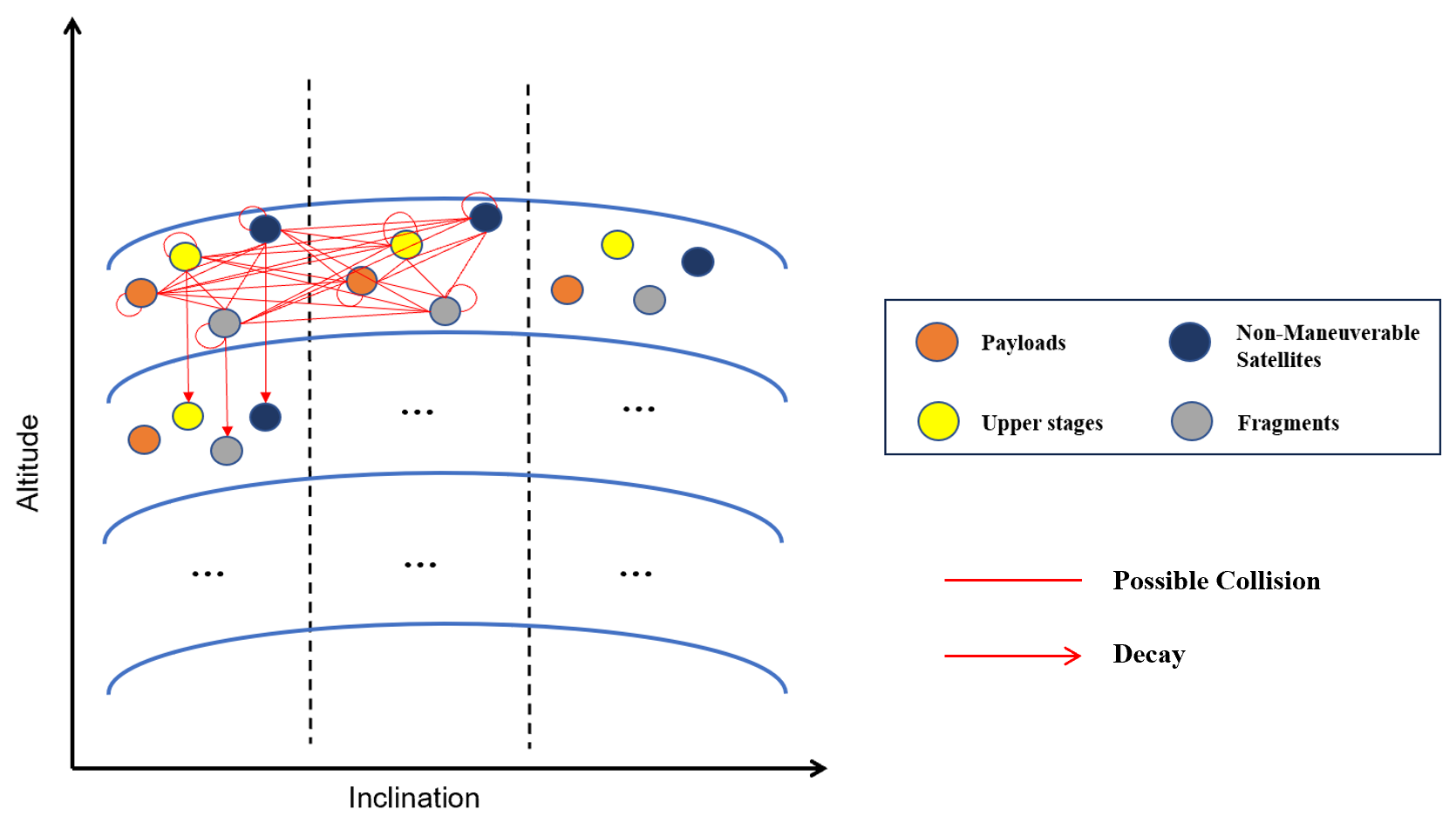
Figure 1: Illustration of the network model for the space environment.

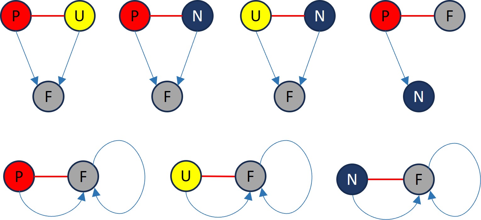
Figure 2: Representative interaction configurations among the nodes.

It is important to underline that the network model allows for multiple representations of the space environment and can accommodate further nodes of different nature, in addition to the ones that were considered in this study. For example, one could insert nodes representing entire constellations or single satellites, or nodes representing fragments or satellites in elliptical orbits. In this paper we focus our attention only on four classes of objects and an orbit shell model.

2.1 Network Dynamics

Once the structure and topology of the network are defined one can derive the following stochastic evolutionary equations, governing the evolution of each node $P_{i}$, $U_{i}$, $N_{i}$ and $F_{i}$:

$$\begin{array}[]{l}x_{P_{i}}(t_{k+1})=x_{P_{i}}(t_{k})-\sum_{j}\left(\Delta^{CAM}_{P_{i}U_{j}}+\Delta^{CAM}_{P_{i}N_{j}}+\Delta^{CAM}_{P_{i}F_{j}}+(1-s_{CAM})\Delta^{CAM}_{P_{i}P_{j}}\right)\\ -\sum_{j}\Delta^{\kappa}_{P_{i}F_{j}}-\Delta^{EOL}_{P_{i}}+\varepsilon^{+}_{P_{i}}-\varepsilon^{-}_{P_{i}}+\Lambda_{i}(t_{k})\\ x_{U_{i}}(t_{k+1})=x_{U_{i}}(t_{k})-\sum_{j}\Delta^{CAM}_{U_{i}P_{j}}-\sum_{j}(\Delta_{U_{i}N_{j}}+\Delta_{U_{i}F_{j}}+\Delta_{U_{i}U_{j}})-\Delta^{ADR}_{U_{i}}+\varepsilon^{+}_{U_{i}}-\varepsilon^{-}_{U_{i}}\\ x_{N_{i}}(t_{k+1})=x_{N_{i}}(t_{k})-\sum_{j}\Delta^{CAM}_{N_{i}P_{j}}-\sum_{j}(\Delta_{N_{i}N_{j}}+\Delta_{N_{i}F_{j}}+\Delta_{N_{i}U_{j}})+\\ \sum_{j}\Delta^{\kappa}_{P_{i}F_{j}}+\Delta^{\gamma}_{P_{i}}-\Delta^{ADR}_{N_{i}}+\varepsilon^{+}_{N_{i}}-\varepsilon^{-}_{N_{i}}\\ x_{F_{i}}(t_{k+1})=x_{F_{i}}(t_{k})-\sum_{j}\Delta^{CAM}_{F_{i}P_{j}}-\sum_{j}(\Delta_{F_{i}N_{j}}+\Delta_{F_{i}F_{j}}+\Delta_{F_{i}U_{j}})-\\ \Delta^{ADR}_{F_{i}}+\varepsilon^{+}_{F_{i}}-\varepsilon^{-}_{F_{i}}+\sum_{j}\Omega^{F_{i}}_{j}\\ \end{array}$$ (1)

with

$$\begin{array}[]{l}\Delta_{S_{i}S_{j}}=\int_{t_{k}}^{t_{k+1}}d\mathcal{N}(\tau_{S_{i}S_{j}}\Delta t_{k})\\ \Delta^{CAM}_{S_{i}S_{j}}=\int_{t_{k}}^{t_{k+1}}d\mathcal{N}((1-s_{CAM})\tau_{S_{i}S_{j}}\Delta t_{k})\\ \Delta^{\kappa}_{S_{i}S_{j}}=\int_{t_{k}}^{t_{k+1}}d\mathcal{N}(\kappa\tau_{S_{i}S_{j}}\Delta t_{k})\\ \Delta^{\gamma}_{S_{i}}=\int_{t_{k}}^{t_{k+1}}d\mathcal{N}(\gamma\Delta^{EOL}_{P_{i}})\\ \Omega^{F_{i}}_{j}=\sum_{l}\left(\zeta^{F_{i}}_{P_{j}U_{l}}\Delta^{CAM}_{P_{j}U_{l}}+\Delta^{CAM}_{P_{j}N_{l}}\zeta^{F_{i}}_{P_{j}N_{l}}+\Delta^{CAM}_{P_{j}F_{l}}\zeta^{F_{i}}_{P_{j}F_{l}}+\Delta^{CAM}_{P_{j}P_{l}}\zeta^{F_{i}}_{P_{j}P_{l}}\right)+\\ \sum_{l}\left(\Delta_{U_{j}U_{l}}\zeta^{F_{i}}_{U_{j}U_{l}}+\Delta_{U_{j}N_{l}}\zeta^{F_{i}}_{U_{j}N_{l}}+\Delta_{U_{j}F_{l}}\zeta^{F_{i}}_{U_{j}F_{l}}+\Delta_{N_{j}N_{l}}\zeta^{F_{i}}_{N_{j}N_{l}}+\Delta_{N_{j}F_{l}}\zeta^{F_{i}}_{N_{j}F_{l}}+\Delta_{F_{j}F_{l}}\zeta^{F_{i}}_{F_{j}F_{l}}\right)\end{array}$$ (2)

where $d\mathcal{N}(\lambda_{S_{i}S_{j}})$ is a jump process with expected value $\lambda_{S_{i}S_{j}}(t_{k},x_{S_{i}}(t_{k}),,x_{S_{j}}(t_{k}))$, $\Delta t_{k}=t_{k+1}-t_{k}$ indicates a given time interval, $\kappa$ accounts for collisions with non-trackable fragments which can disable an active payload, $s_{CAM}$ indicates the probability of successfully implementing collision avoidance maneuvers, and $\Delta_{P_{i}}^{EOL}$ indicates the number of payloads subject to Post Mission Disposal (PMD). Payload are removed at a given time $t_{PMD}$ after launch, if PMD is successful. The use of Poisson processes was studied by [32] who demonstrated that it well capture the historical distribution of collisions.

The two indexes $i$ and $j$ indicate a particular site, defined by a combination of an orbit shell and an inclination bin. We also included Active Debris Removal through the factors $\Delta^{ADR}_{F_{i}}$, $\Delta^{ADR}_{N_{i}}$ and $\Delta^{ADR}_{U_{i}}$. Each $\Delta^{ADR}$ is the number of objects of a given species removed at each time step. As it will be explained later the nodes affected by ADR can be chosen so that one can remove the most critical objects. The factor $\gamma$ indicates the failure rate in performing PMD, resulting in objects in $P$ nodes transitioning to $N$ nodes. The small collision factor $\kappa$, quantifies the impacts of small fragments between 1 cm and 10 cm on payloads, leading to a transition of objects from $P$ nodes to $N$ nodes. Following [38], we assumed that collisions with small fragments are $\kappa$ times more frequent than normal collisions with larger objects. The mean collision rate $\tau_{S_{i}S_{j}}$ between node $S_{i}$ and node $S_{j}$ indicates how many objects of a given class are involved in a collision in a given time interval. The function $\Lambda_{i}(t)$ is the number of new payloads, launched with a rate defined by a given launch traffic model that forecasts the frequency of new launches over a given period. The quantity $\Delta^{EOL}_{S_{i}}$ is the number of payloads performing PMD over a given period. The quantity $\varepsilon_{S_{i}}^{-}$ represents the outflow from node $S_{i}$, while $\varepsilon_{S_{i}}^{+}$ denotes the inflow to node $S_{i}$, both resulting from changes in the distribution of objects due to orbital evolution. Function $\Omega^{F_{i}}_{j}$ computes the inflow to node $F_{i}$ of the fragments generated from collisions with nodes $P_{j},U_{j},N_{j}$ and $F_{j}$, as shown in Figure 2, where $\zeta^{F_{i}}_{S_{j}S_{l}}$ indicates the fragments generated by the catastrophic collisions between node $S_{j}$ and node $S_{l}$ that flow to node $F_{i}$. Therefore, $\Delta t_{k}\tau_{S_{j}S_{l}}\zeta^{F_{i}}_{S_{j}S_{l}}$ indicates the new fragments flowing to node $F_{i}$ after the collision between node $S_{j}$ and node $S_{k}$ in the given time interval $\Delta t_{k}$. Considering satellite maneuverability, the fragments generated by the collisions with payloads, need to be scaled by $1-s_{CAM}$. Let $\mathbf{X}_{k}=[x_{P_{1}},x_{U_{1}},x_{N_{1}},x_{F_{1}}...,x_{P_{i}},x_{U_{i}},x_{N_{i}},x_{F_{i}},...,x_{P_{n}},x_{U_{n}},x_{N_{n}},x_{F_{n}}]^{T}$ represent the vector that contains all the nodes $x_{S_{i}}$, with $S\in\{P,U,N,F\}$ and $i=1,...,n$, then a more compact form of the evolutionary equations in (1) is:

$$\mathbf{X}_{k+1}=\mathbf{X}_{k}+\mathbf{Y}(\mathbf{X}_{k})+\mathbf{g}(t_{k})$$ (3)

where $\mathbf{Y}(\mathbf{X}_{k})$ contains the interactions among nodes (collisions and orbit change) and satellite failures, while $\mathbf{g}(t_{k})$ contains all time dependent terms, such as the launch traffic model $\Lambda_{i}(t_{k})$ and end of life $\Delta^{EOL}_{S_{i}}$. The launch traffic model, the collision model, and the decay model, will be introduced in the following sections.

The evolutionary model in (1) is a stochastic version of what is commonly known as source-sink model. The key difference with respect to previous works [10] is that we derived the evolutionary equations from the structure of the network. This also differentiates our approach from previous network representations of the space environment [20] that use network theory as a post processing analysis tool.

2.1.1 Launch Traffic Model

The launch traffic model is based on historical launch data and estimates the future launch rates. Historical data to fit the model are taken from DISCOSWeb. The total number of objects launched in a certain year is given by an exponential logistic curve of the form [44]

$$\Lambda(t)=n_{0}+\sum_{i=1}^{M}\frac{A_{i}e^{d_{i}(t-t_{i})}}{b_{i}+e^{-c_{i}(t-t_{i})}}$$ (4)

where $t$ is expressed in years and the parameters $n_{0}$, $A_{i}$, $b_{i}$, $c_{i}$, $d_{i}$, and $t_{i}$ control the shape of the curve. These parameters can be selected based on historical trends and predicted future increases in launch traffic. Launched objects are either payloads, upper stages, or mission related objects. The proportion of each is based on the most recent years of launches. For each object class, orbital and physical parameters of historical launches are fit to a Gaussian Mixture Model (GMM). A separate GMM was fit to the distribution of semimajor axis and inclination, and to physical parameters like mass, cross section area, and length. The increase in objects with a given set of physical properties sampled from each GMM, follows the model in (4). Hence, for each site in the network, one can derive the expected number of objects with altitude and inclination specific to that site, from the GMM, and increase them over time following (4). Figure 3 shows example forecasts for $M=1$ and for the number of objects launched into Low Earth Orbit. Also shown are the parameters used to derive the different trends. The choice of parameters reflects different qualitative assumptions on how the number of objects launched will evolve in future. The blue line suggests a steadier increase in new launches in future following the sharp upward trend since 2023 that representing a timely restriction on launch activity, whereas the black and red lines suggest that the number of objects reaching a plateau occurs later, at different levels, with the black line plateauing around 2032 and the red line around 2050.

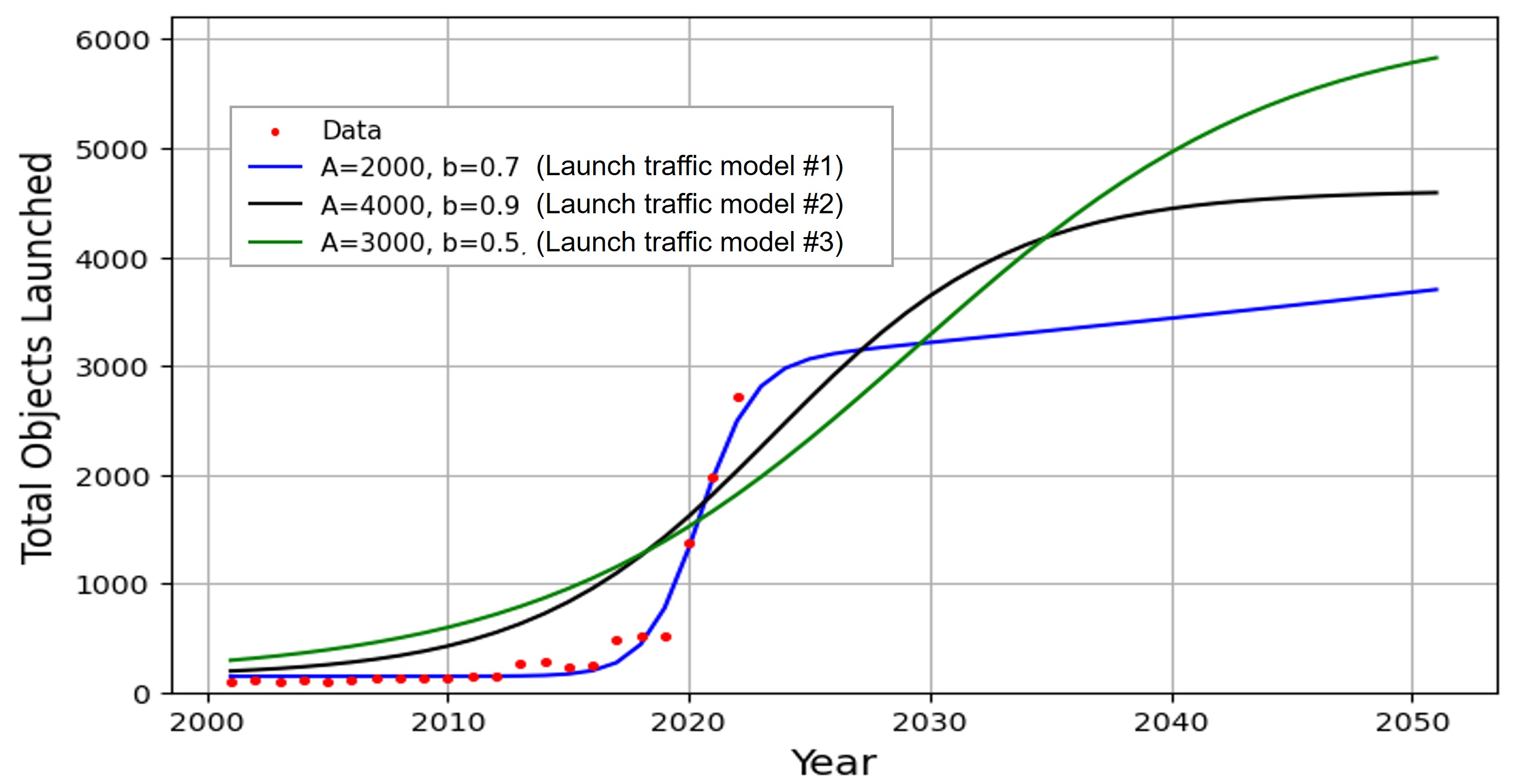
Figure 3: Model of number of objects launched to LEO

The GMM is fit to the altitude and inclination of historical launches. The launch model samples points from this distribution to add to the network. These samples are continuous in altitude and inclination, which can then be assigned to relevant nodes within each altitude and inclination site.

2.1.2 Collision Rates

The mean collision rate between node $S_{i}$ and node $S_{j}$ follows the kinetic theory of gas and is defined as

$$\tau_{{S_{i}}{S_{j}}}=\frac{n_{S_{i}}n_{S_{j}}\Delta v_{l}\sigma_{{S_{i}}{S_{j}}}}{\max(V_{S_{i}},V_{S_{j}})}$$ (5)

where $n_{S_{i}}$ is the number of objects in node $S_{i}$, and the volume of a generic node $S$ defined by an orbit shell of thickness $dr$ and inclination bin $i\in[i_{min},i_{max}]$ is:

$$V_{S}=4\pi\sin(i_{max})\left[(r+dr)^{3}-r^{3}\right]/3$$ (6)

Note that if $pi/2\in[i_{min},i_{max}]$ then $i_{max}=pi/2$ and for $i_{max}\wedge i_{min}>pi/2$ we use $i=pi-i$. Given $\sigma_{{S_{i}}{S_{j}}}$ and $\Delta v_{l}$, the collision cross-sectional area [15] and the mean relative collision velocity between the two nodes, then [18]:

$$\left\{\begin{split}\sigma_{{S_{i}}{S_{j}}}&=\pi\left(d_{S_{i}}+d_{S_{j}}\right)^{2}/4\\ \Delta v_{l}&=\frac{14\sqrt{2}}{15}\sqrt{\frac{\mu}{r}}\end{split}\right.$$ (7)

where $r_{l}$ is the mean radius of the orbit shell, $d_{S_{i}}$ and $d_{S_{j}}$ are the average diameters of the objects in nodes $S_{i}$ and $S_{j}$, $i_{S_{i}}$ and $i_{S_{j}}$ are the average inclinations of the objects in nodes $S_{i}$ and $S_{j}$. The number of collisions between node $S_{i}$ and node $S_{j}$ is sampled from a Poisson distribution

$$\Delta_{S_{i}S_{j}}=\int_{t_{k}}^{t_{k+1}}d\mathcal{N}(\tau_{S_{i}S_{j}}\Delta t_{k})$$ (8)

to form the collision pairs between nodes $S_{i}$ and node $S_{j}$, $\Delta_{S_{i}S_{j}}$ objects are selected from each node if $S_{i}\neq S_{j}$, and $2\Delta_{S_{i}S_{i}}$ objects from one node if $S_{i}=S_{j}$. A sampling strategy without replacement is employed according to the cross-section area distribution of objects, where the probability of object $q$ in node $S_{i}$ being selected is

$$p_{q}=\frac{r^{2}_{q}}{\max(r^{2}_{1},...,r^{2}_{q},...,r^{2}_{n_{S_{i}}})}$$ (9)

where $r_{q}$ indicates the radius of object $q$. Figure 4 provides an example for illustrating the basic idea of the proposed sampling strategy. Assuming a node contains 10 objects, where 7 objects have a radius of 0.2 m, 2 objects have a radius of 0.4 m, and 1 object has a radius of 1 m. Figure 4(a) illustrates the radius distribution of these 10 objects, while Figure 4(b) shows the sampling probabilities. Notably, the object with the largest radius of 1 meter has the highest probability of being selected at 0.625, even though it accounts for only 1 out of the 10 objects.

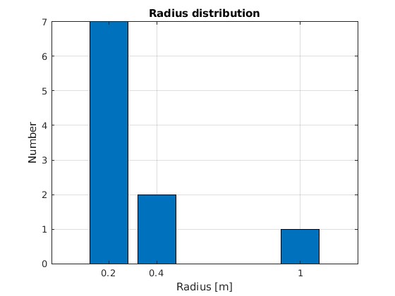
(a) Radius distribution.

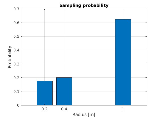
(b) Sampling probability.

Figure 4: Example for the sampling strategy.

Subsequent to a collision, the approximated number of the generated fragments is calculated by [14]

$$\zeta_{{S_{i}}{S_{j}}}(L_{c})=0.1M_{{S_{i}}{S_{j}}}^{0.75}L_{c}^{-1.71}$$ (10)

where $L_{c}$ indicates the minimum size of the fragments. Given that a catastrophic collision occurs when the impact kinetic energy-to-target mass ratio exceeds $40\text{\,}\mathrm{J}\mathrm{/}\mathrm{g}$, $M_{{S_{i}}{S_{j}}}$ is defined as the mass of both objects in a catastrophic collision, while in the case of a non-catastrophic collision, the value of $M_{{S_{i}}{S_{j}}}$ is defined as the mass of the smaller object multiplied by the collision velocity. The physical parameter distribution and the velocity distribution of the resulting fragments can be computed by NASA’s breakup model [14]. Considering orbital elements of the fragments, only a portion of the fragments from each collision flows to $F_{k}$, therefore, the notation $\zeta^{F_{k}}_{S_{i}S_{j}}$ is introduced to represent the fragments generated from the collision between node $S_{i}$ and node $S_{j}$ that flow to node $F_{k}$.

2.1.3 Decay Model

Building on the averaging perturbation technique proposed by [26], a time-explicit analytic approximate solution [13] for the motion of low-Earth-orbiting satellites is used. Given $[a_{k},e_{k}]$ at the current time $t_{k}$, the $a_{k+1}$ after $\Delta t_{k}$ is

$$\begin{split}a_{k+1}&=\frac{a_{k}}{\beta_{k}^{2}}\tan^{2}\left[\arctan(\beta_{k})-\beta_{k}n_{k}a_{k}C_{k}\Delta t_{k}\right]\\ e_{k+1}&=\frac{2}{\sqrt{3}}\tan\left[\arctan(\beta_{k})-\beta_{k}n_{k}a_{k}C_{k}\Delta t_{k}\right]\end{split}$$ (11)

where

$$C_{k}=\frac{1}{2}C_{d}\frac{A}{m}\rho,\qquad\bar{n}_{k}=\sqrt{\frac{\mu}{a_{k}^{3}}},\qquad\beta_{k}=\begin{cases}\frac{\sqrt{3}}{2}e_{k},&e_{k}\neq 0\\ 1,&e_{k}=0\end{cases}$$ (12)

where $\rho$ indicates the atmospheric density. This paper employs the Jacchia-Bowman 2008 (JB2008) density model [5], an empirical model derived from historical atmospheric density data to represent the average statistical behavior of the atmosphere under varying solar and geomagnetic influences [13]. Assuming the altitude of object $q$ is $h^{q}(t_{k+1})$ at $t_{k+1}$, the quantity $\omega^{q}_{{S_{i}}{S_{j}}}(t_{k+1})$ is an indicator that says if object $q$ in node $S_{i}$ can flow from node $S_{i}$ to the node $S_{j}$ within $\Delta t_{k}$:

$$\omega^{q}_{{S_{i}}{S_{j}}}(t_{k+1})=\begin{cases}1,\quad if\;\underline{h}_{Sj}<h^{q}(t_{k+1})<\overline{h}_{Sj}\\ 0,\quad else\end{cases}$$ (13)

where $\overline{h}_{S_{j}}$ indicates the upper bound of the orbital shell of node $S_{j}$, respectively. The flow from node $S_{i}$ to node $S_{j}$ is

$$\varepsilon_{S_{i}S_{j}}(t_{k+1})=\sum^{n_{S_{i}}}_{q=1}\omega^{q}_{{S_{i}}{S_{j}}}(t_{k+1})$$ (14)

Therefore, the outflow $\varepsilon_{S_{i}}^{-}$ and inflow $\varepsilon_{S_{i}}^{+}$ are

$$\begin{cases}\varepsilon^{-}_{S_{i}}=\sum^{n}_{j\neq i}\varepsilon_{S_{i}S_{j}}(t_{k+1})\\ \varepsilon^{+}_{S_{i}}=\sum^{n}_{j\neq i}\varepsilon_{S_{j}S_{i}}(t_{k+1})\\ \end{cases}$$ (15)

2.1.4 Treatment of Elliptical Orbits

Considering an object $q$ with an elliptical orbit, the distribution to shells should be weighted according to the residence time in each orbital shell [25].

$$g^{q}(\theta,e)=2\arctan\left[\left(\frac{1-e}{1+e}\right)^{\frac{1}{2}}\tan\frac{\theta}{2}\right]-\frac{e(1-e^{2})^{\frac{1}{2}}\sin\theta}{1+e\cos\theta}$$ (16)

where $e$ is the eccentricity. Therefore, the proportion of residence time in orbital shell $\nu$ is

$$w^{q}_{\nu}=\frac{[g^{q}(\theta_{\nu+1},e_{k+1})-g^{q}(\theta_{\nu},e_{k+1})]}{\pi}$$ (17)

where $\theta_{\nu}$ is the phase angle corresponding to where the orbit crosses the lower edge of the $\nu$-th shell, For each object $q$, a sampling strategy without replacement is used to randomly select the orbital shell where the object is most likely to be found in terms of the $w^{q}_{\nu}$ for each shell.

Therefore, with the consideration of elliptical orbits, the basic idea for calculating $\varepsilon_{S_{i}S_{j}}$ is to compute the difference in the number of objects in each node before and after decay according to the distribution of the objects. For objects with the same species in $\omega$-th inclination bin, the approximated number of objects in $\nu$-th shell is

$$\delta n^{(\omega)}_{\nu}=\sum_{l\in\mathcal{L}_{\omega}}\sum^{n_{S_{l}}}_{q=1}w^{q}_{\nu}$$ (18)

The set $\mathcal{L}_{\omega}=\{\omega+(\nu-1)n_{\omega}\mid\nu=1,2,\dots,n_{\nu}\}$, where $n_{\omega}$ and $n_{\nu}$ represent the number of inclination bins and orbital shells, respectively. Therefore, one can start with the inflow $\epsilon^{(\omega)+}_{\nu}$ for the highest shell set to 0, and then iteratively compute the outflow $\epsilon^{(\omega)-}_{\nu}$ for each shell and the corresponding inflow of each lower shell.

3 Validation of the Network Dynamics

In this section, we compare NESSY against an already validated evolution model: MOCAT-MC [13]. The initial condition for both NESSY and MOCAT-MC is the population of resident objects in LEO at the beginning of 2023, available from SatCat TLEs [37] and ESA DISCOS [30]. The portion of the space environment covered in this comparison, spans a range of altitudes from 200 to 2200 km. The composition of the initial population is reported in Table 1. In the network model the population is divided into four species, for each inclination bin and orbit shell.

Table 1: Composition of the initial population in March 2023, from the ESA DELTA model.

Payloads	Upper-stages	Fragments	Non-maneuverable satellite	Total
5471	1111	9804	2440	18 826

3.1 Long Term Evolution Results

Both MOCAT-MC and NESSY use the same atmospheric model and for this comparison we did not include any future launch. For NESSY we assumed that: the PMD was 5 years, i.e. a new payload was removed from the environment after 5 years if still active, and the PMD failure rate was 5%. This failure rate results in a proportion of payloads becoming non-maneuverable satellites. The small collision factor $\kappa$, which quantifies the impacts of small fragments between 1 cm and 10 cm on payloads, was set to 5.3, as in [38]. The success rate of collision avoidance maneuvers, $s_{CAM}$, was set to 99.9 %. The new fragments have a diameter larger than 10 cm were considered. The altitude range was partitioned in orbital shells with a width of 50 km. The inclination range, spanning from $0^{\circ}$ to $180^{\circ}$, was partitioned in inclination bins with an angular size of 60^∘. The values used in NESSY for this comparative test against MOCAT-MC are reported in Table 2, while those for MOCAT are reported in Table 3.

Table 2: Settings of NESSY for the comparative analysis with MOCAT-MC.

Parameter name	Value
Time step	30 days
Propagation time	100 years
Inclination bin size	60 deg
Altitude shell size	50 km
$s_{CAM}$	99.99 %
$\gamma$	5 %
Payloads mission lifetime	5 years
Small collisions factor	5.3

Table 3: Settings of MOCAT-MC for the comparative analysis with NESSY.

Parameter name	Value
Time step	5 days
Propagation time	100 years
PMD successful rate	95 %
$s_{CAM}$	99.99 %
Explosion probability per day	0
Payloads operational lifetime	5 years

Figure 5 shows the evolution of the four species modeled in NESSY plus the whole population. The network dynamics was propagated for 100 years, with a 30 day time step, and each propagation was repeated for 60 times to compute mean and variance. In Figure 5, the blue line represents the average of the runs while the gray area is the 1-sigma variance of the runs. Oscillations in the evolution of all the species are due to the Jacchia-Bowmann atmospheric model, which is characterised by a periodic value of the atmospheric density, following the Sun cycle. The entire payload population disappears within the first 10 years of the simulation, because of small collisions, failure rate and post-mission disposal. This huge decrease corresponds to an initial increase in N (non-maneuvrable objects). The only class constantly increasing is the fragments one (F), because of collisions happening between objects. Figure 7(a) shows the cumulated number of collisions over time.

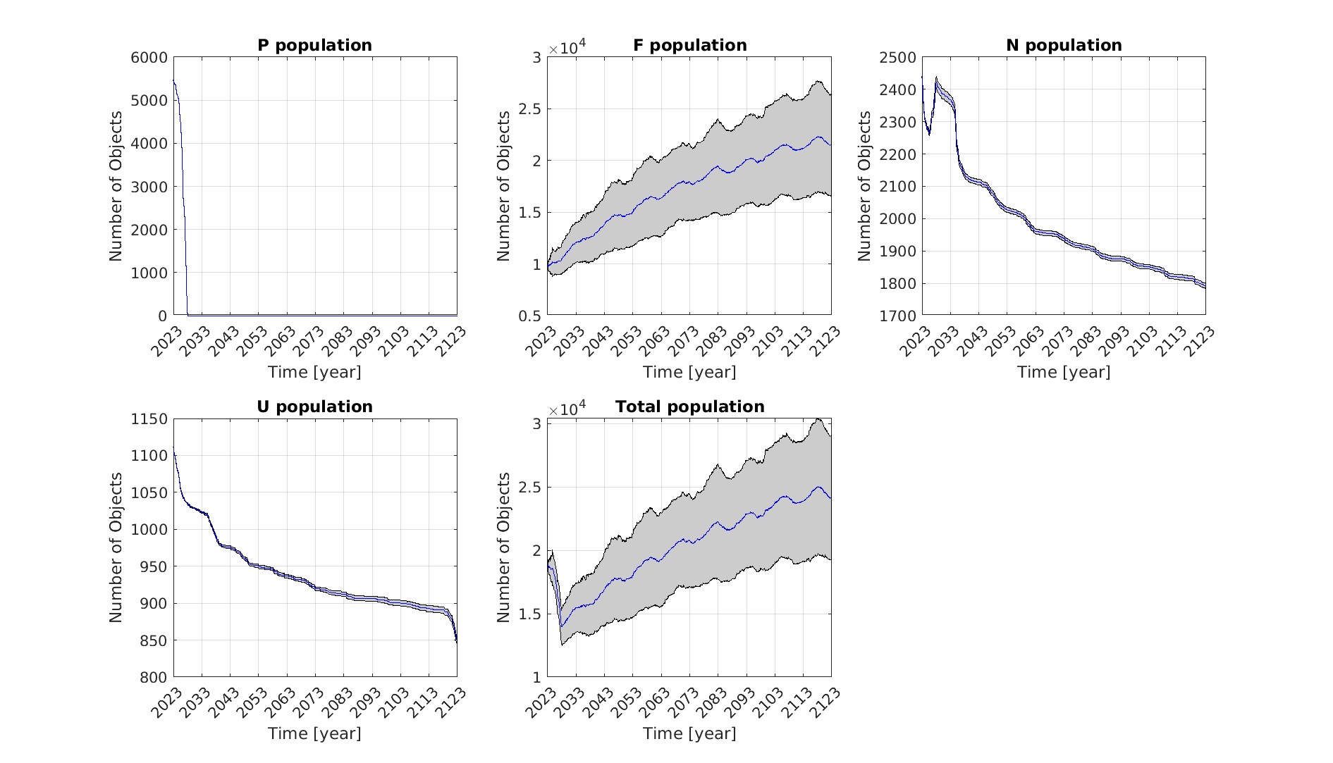
Figure 5: Evolution of the population propagated with NESSY with 60 deg inclination bins, 50 km altitude shells and a 30 day time step.

For comparison Figure 6 shows the evolution of the same initial population propagated with MOCAT-MC. The propagation is for 100 years, with the same atmospheric model and a time step of 5 days. Every propagation was repeated for 60 times. The average trends (blue curves) are reported together with the standard deviation (gray area) for all the object classes. We can see that the trends of the different objects are very similar to those of NESSY. The total population after 100 years is very close as well, differing by just a few hundred objects (mainly fragments). The cumulative number of collisions is reported in Figure 7(b). The final number is close to 40 for both models, although NESSY presents a steep increase at the start and then a linear increase with a slope slightly lower than MOCAT-MC. On the contrary, MOCAT-MC has a linear increase with constant slope from the the start. The difference in the cumulated collisions trend between NESSY and MOCAT is because of the small collisions with payloads in NESSY. This is clear because the difference in trend is present just for the initial period when payloads are still in the environment, while after that, it becomes linear as in MOCAT. On the other hand NESSY is not tracking small fragments and their impact on defunct satellites. This is point that will be addressed in future works.

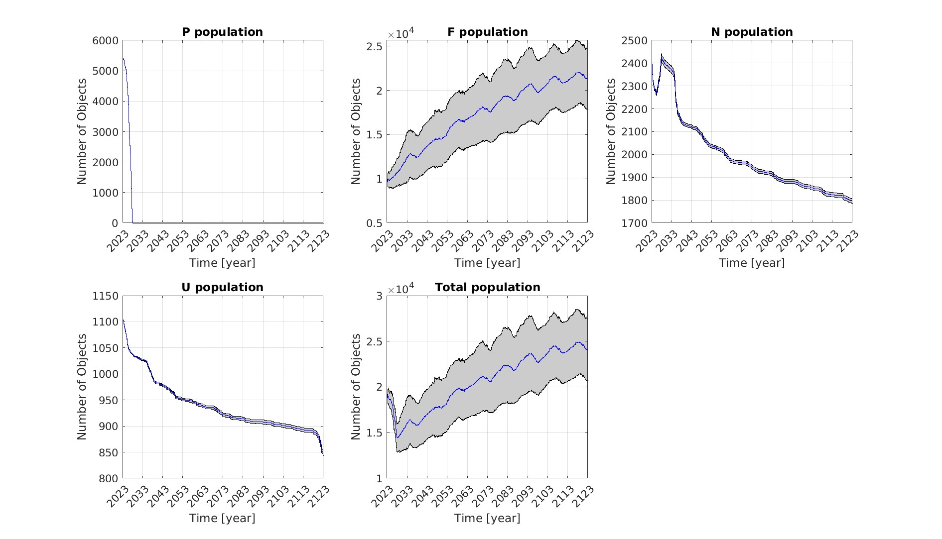
Figure 6: Evolution of the population propagated with MOCAT-MC with a 5 day time step.

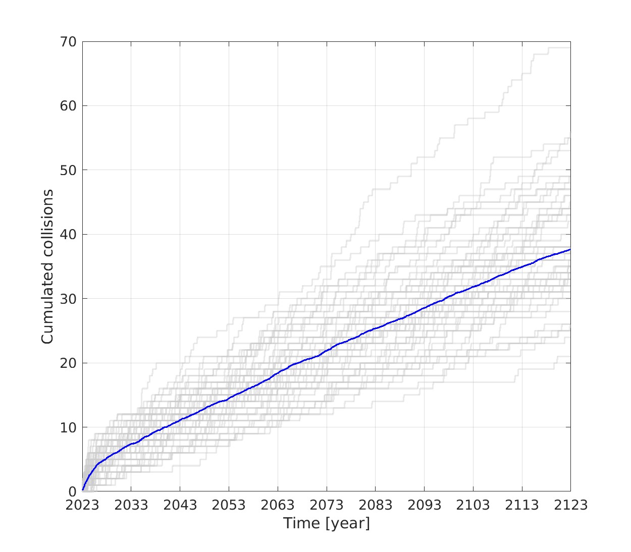
(a)

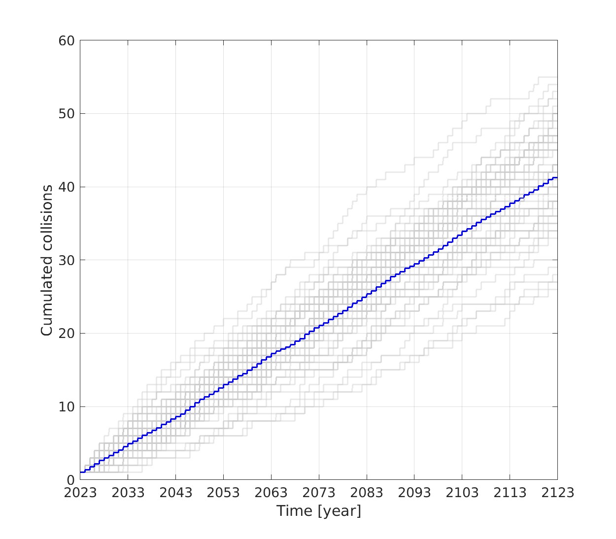
(b)

Figure 7: a) NESSY cumulated number of collisions for 30 deg inclination bins, 50 km altitude shells, 30 day time step and 60 independent runs; b) MOCAT-MC cumulated number of collisions, for a 5 day time step and 60 independent runs.

3.2 Sensitivity Analysis

In this section we present a sensitivity analysis of both NESSY and MOCAT-MC to some of the discretisation parameters: inclination bins, time step, orbit shell size. Figure 8 reports the comparison of the evolution of each object class for different time steps. The trends are very close to each other, and are closer for smaller time steps. Figure 9 instead compares the average cumulative number of collisions for different time steps. From the figure it is apparent that the NESSY has a sharper initial increase and lower slope, although the final number of collisions is similar over the 100 years of simulation.

Figure 10(a) shows the total number of objects in the final population after 100 years for different combinations of altitude shells and inclination bins, while Figure 10(b) shows the final number of non-manoeuverable objects for the same combinations of altitude shells and inclination bins. In the figure the first number next to each blue dot is the size of the inclination bin and the second number is the size of the altitude shell. Note that up to about 400 nodes the size of the final population increases with the number of nodes. From 400 nodes to 1,000 the final population remains roughly the same with a small variation around 25,500 objects. Also the final number of N objects remains around 1,791.

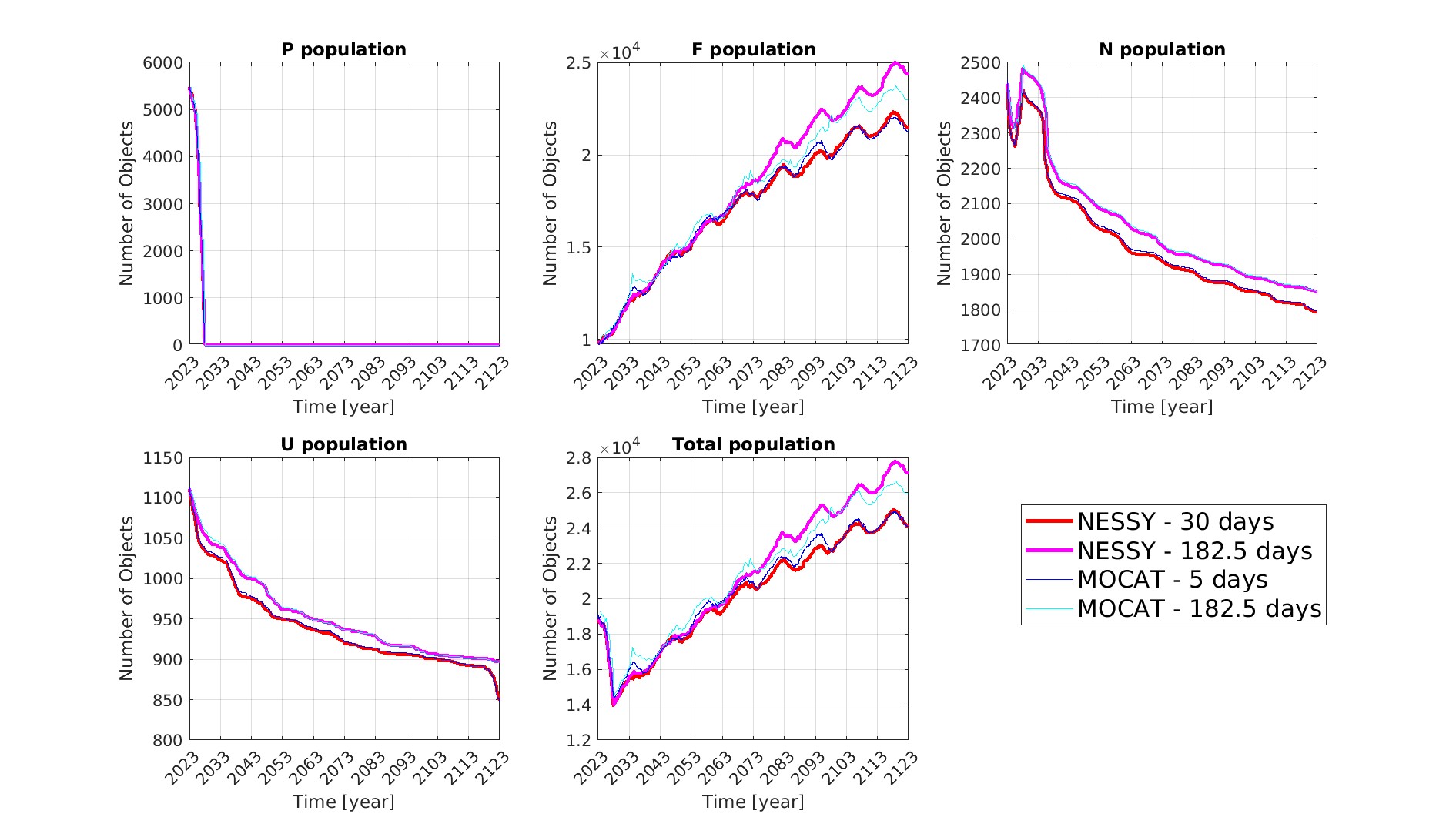
Figure 8: Comparison between the mean evolution of the population propagated with NESSY (with 60 deg inclination bins and 50 km altitude shells) and MOCAT-MC, over 60 independent runs.

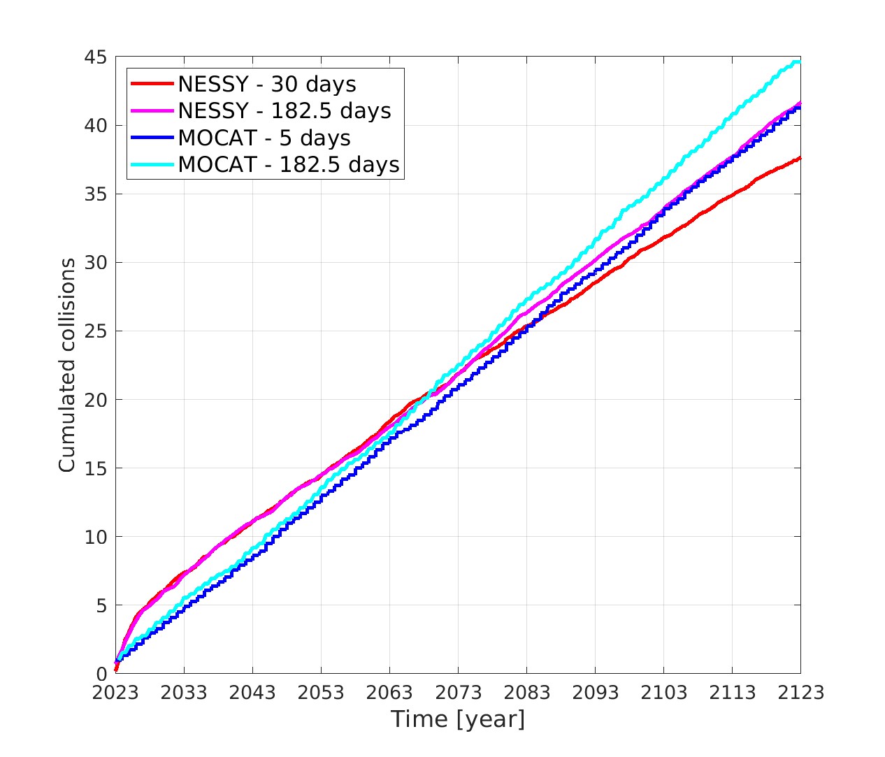
Figure 9: Comparison between the mean cumulative number of collisions computed with NESSY (with 60 deg inclination bins and 50 km altitude shells) and MOCAT-MC, over 60 independent runs.

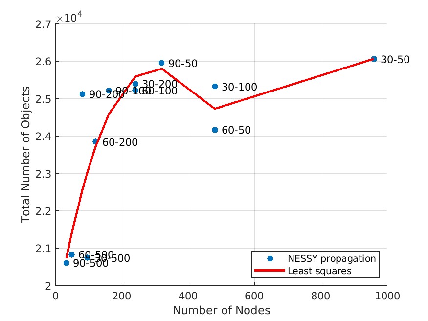
(a) Total number of objects in the final population vs number of nodes in the network.

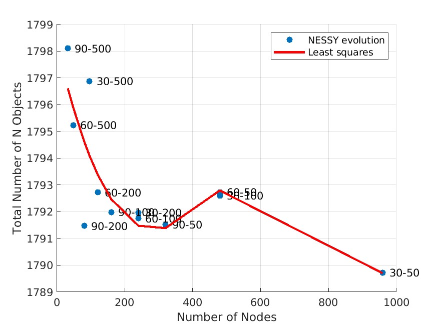
(b) Number of objects of class N in the final population vs number of nodes in the network.

Figure 10: Average number of objects for different combinations of altitude shell and inclination bin: 60 independent runs, 100 years simulation, 182.5 day time step. The red line reports the least squares regression for both cases.

4 Case Studies

This section shows how NESSY can be used to assess the impact of the launch traffic and debris mitigation policies on the evolution of the space environment. The initial population is the same as in previous sections, see Table 2, and the launch traffic model is the one introduced in Section 2.1.1. All the results in this section were obtained with a network where each node represents a 60 deg inclination bin and a 50km altitude shell.

We start by showing the distribution of the collision rate for the baseline case of no future launches that we analysed in the previous section. Figures 11(a), 11(b), 12(a), 12(b), 13(a), 13(b) represent the evolution of the collision rate and distribution of objects, respectively, at 3 instants of time along the 100 year propagation: year 2023, 2073 and 2123. These plots show how the collision rate changes with the evolution of the distribution of the number of objects. As it is clear from the plots, the main contribution to the collision rate comes from the fragments population. This result is consistent with the results in [31].

(a) Collision rate distribution by shell and entire population distribution through nodes.

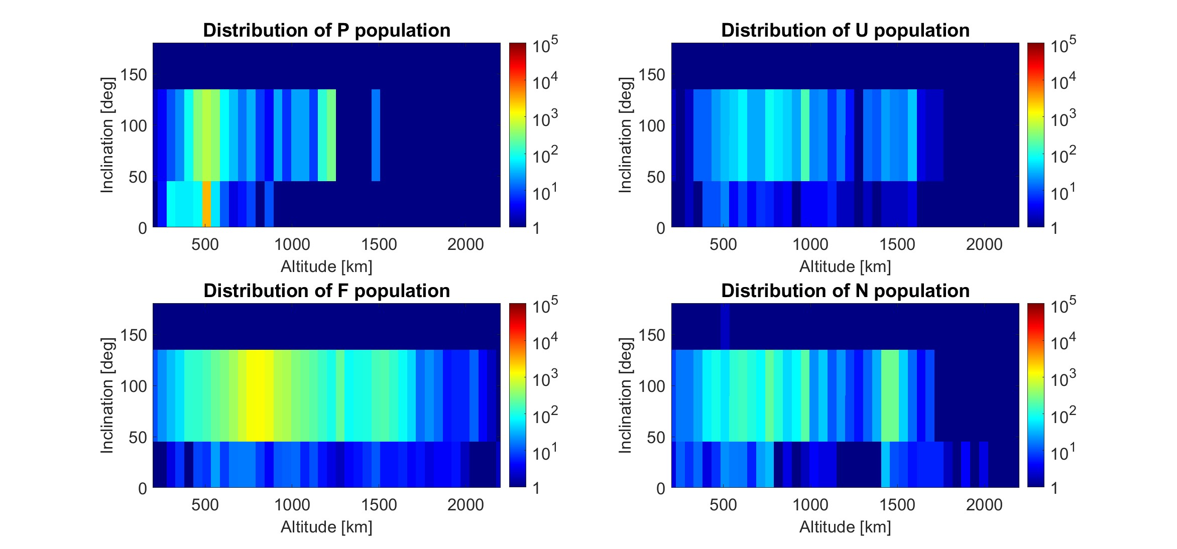
(b) Objects distribution by classes through nodes.

Figure 11: Distribution of the collision rate and number of objects in year 2023.

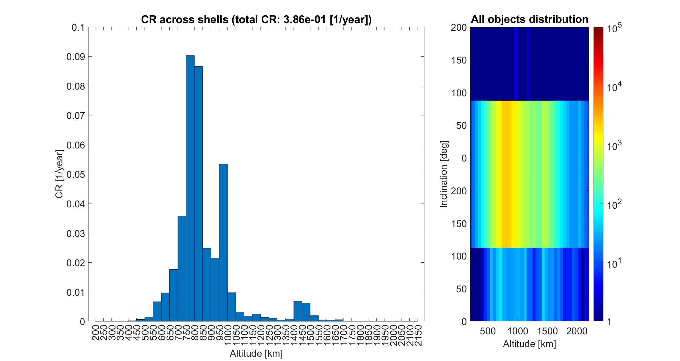
(a) Collision rate distribution by shell and entire population distribution through nodes.

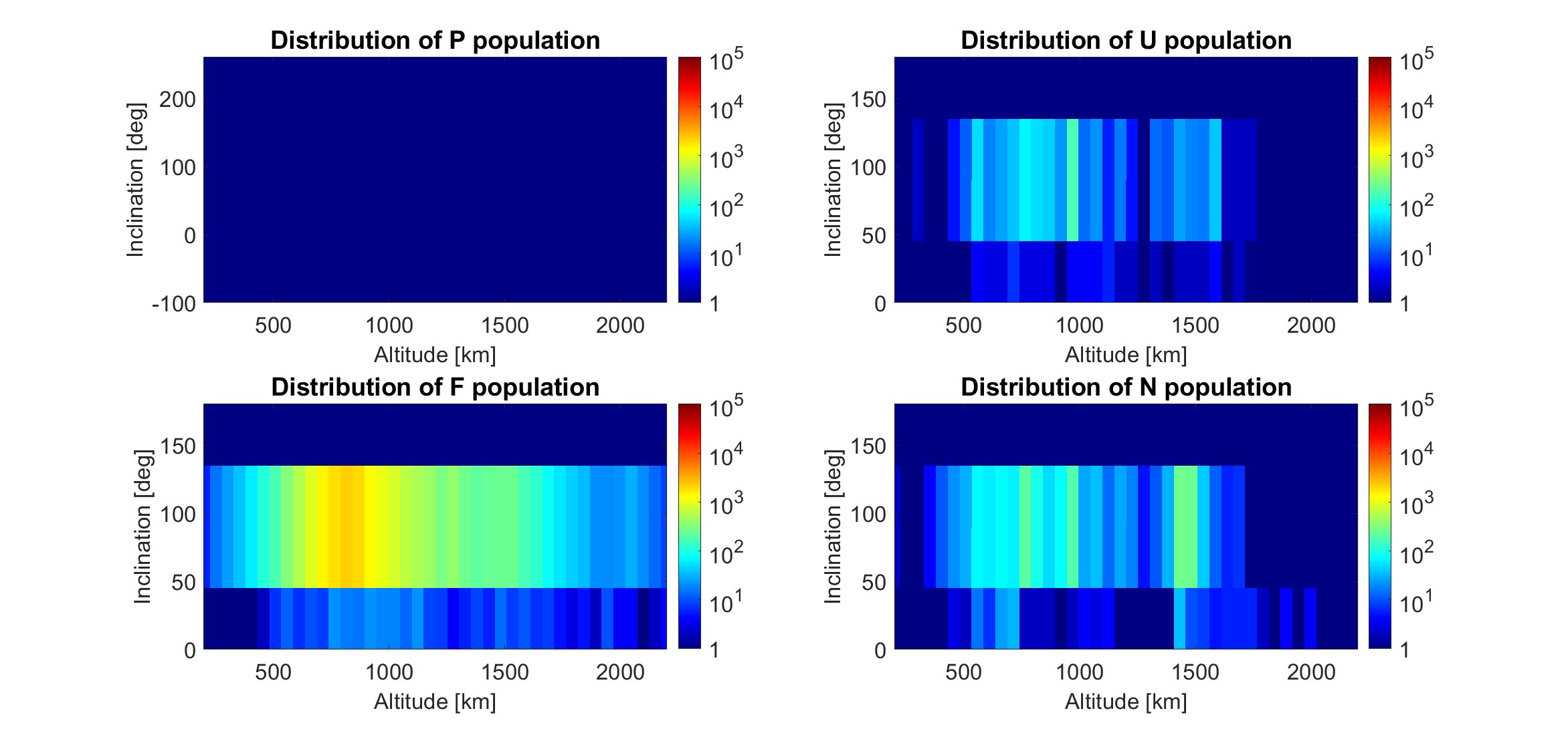
(b) Objects distribution by classes through nodes.

Figure 12: Distribution of the collision rate and number of objects in year 2073.

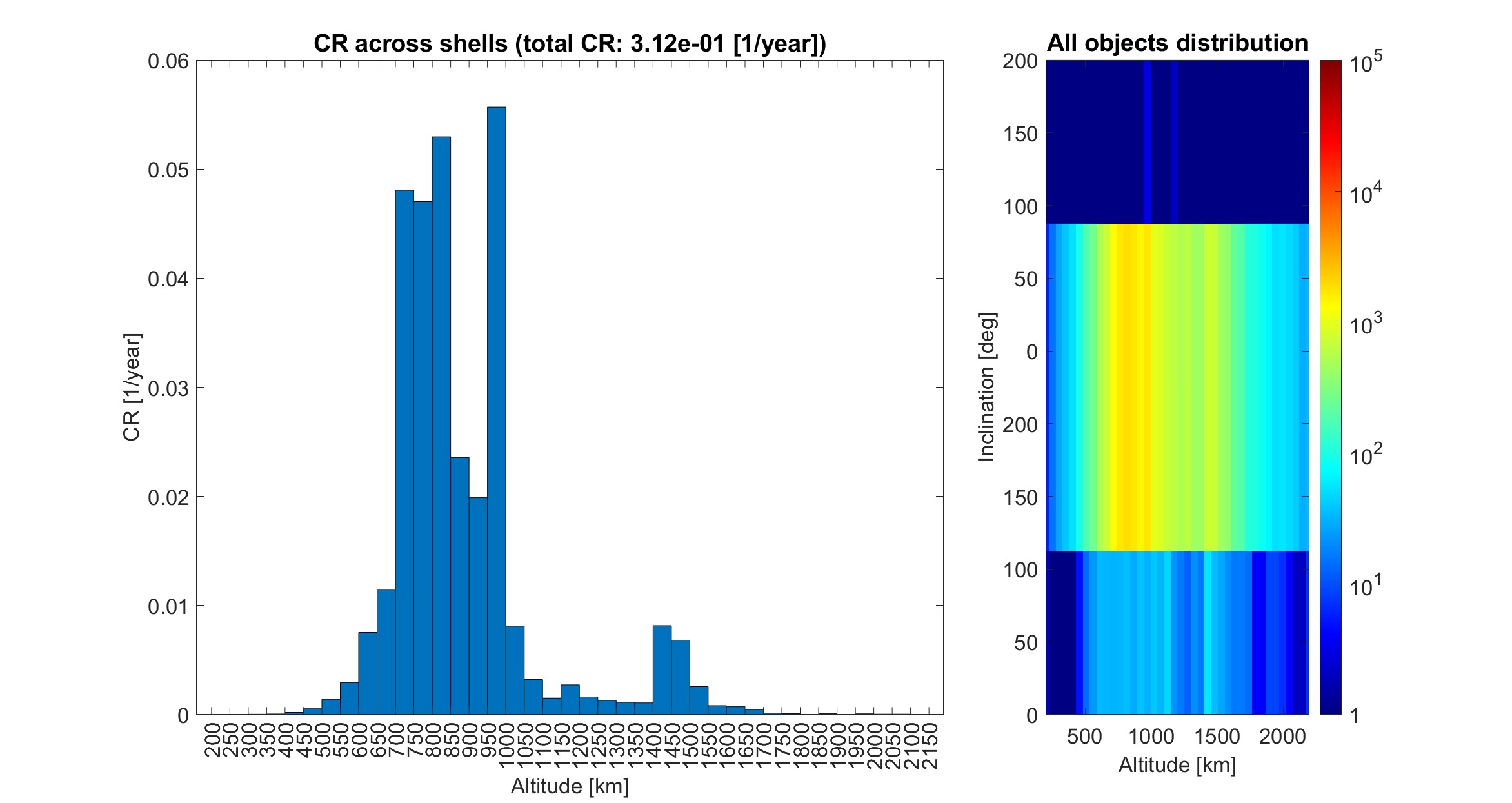
(a) Collision rate distribution by shell and entire population distribution through nodes.

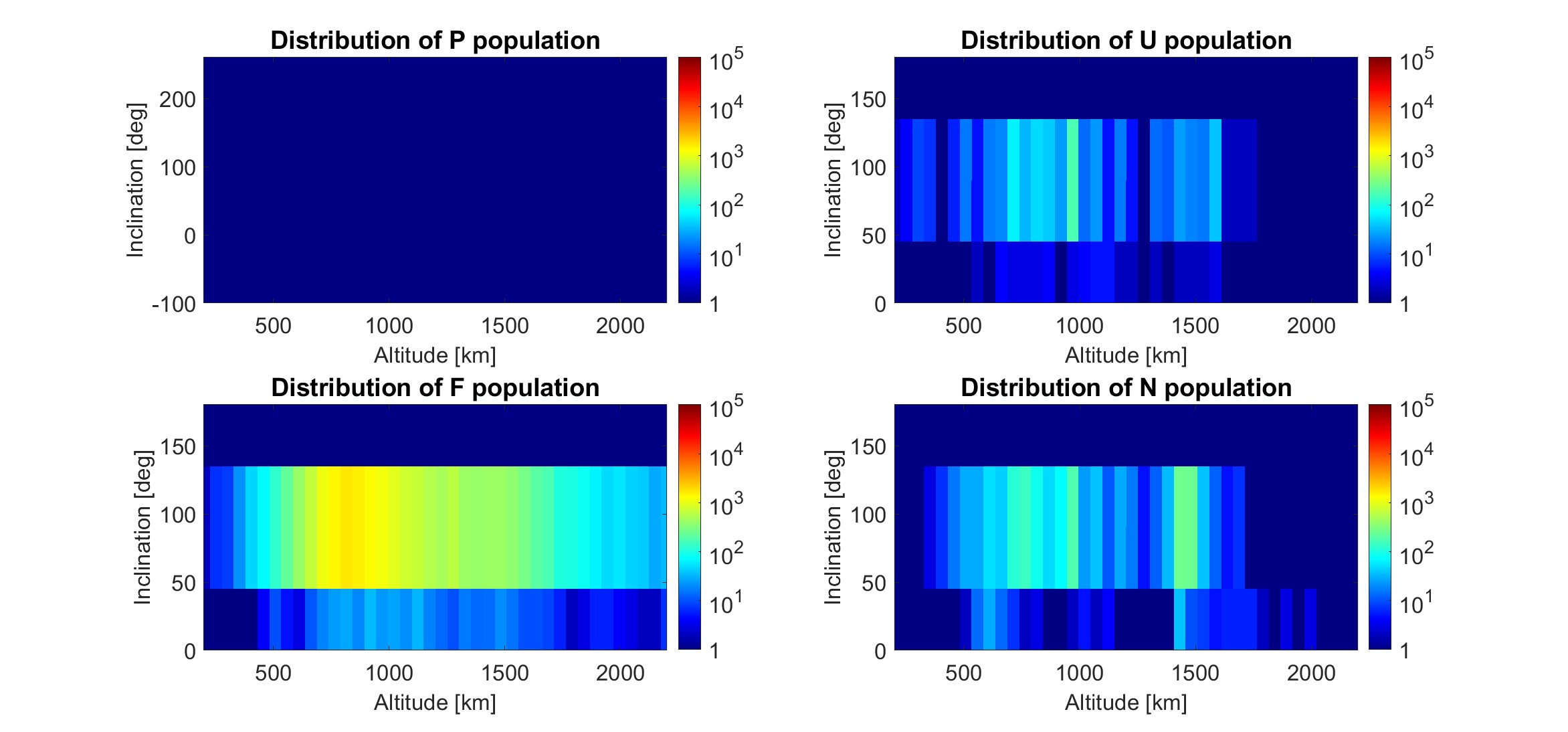
(b) Objects distribution by classes through nodes.

Figure 13: Distribution of the collision rate and number of objects in year 2123.

4.1 Impact of Future Launch Traffic

Figures 14 and 15 compare the evolution of different species and the cumulated collisions over 40 years, for the three launch models (LM) introduced in section 2.1.1. Compared to the baseline case, the effect of the launch traffic is a significant increase in all species with the increase in the number of collisions changing from linear to exponential. Since the launch models presented in this paper incorporate the addition of upper stages and mission-related objects with each new launch, all three models lead to an increase in the numbers of upper stages and non-maneuverable satellites, while the number of payloads eventually reaches either a plateau or continues with a linear increase.

The time variation of the number of payloads can be further explained by computing the expected increment in the number payloads computed with equations (1). Assuming that there is no decay of payloads due to atmospheric drag, the expected value of $\Delta x_{P_{i}}$ at time $t_{k}$ is

$$\begin{array}[]{l}\mathbb{E}(\Delta x_{P_{i}})=-\sum_{j}(1-s_{CAM})\left(\tau_{P_{i}U_{j}}\Delta t_{k}+\tau_{P_{i}N_{j}}\Delta t_{k}+\tau_{P_{i}F_{j}}\Delta t_{k}+(1-s_{CAM})\tau_{P_{i}P_{j}}\Delta t_{k}\right)\\ -\sum_{j}\kappa\tau_{P_{i}F_{j}}\Delta t_{k}-\Delta^{EOL}_{P_{i}}+\Lambda_{i}\end{array}$$ (19)

then the evolution equation of payloads can be simplified to

$$\dot{x}_{P_{i}}=-\hat{\gamma}x_{P_{i}}+\lambda$$ (20)

where $\hat{\gamma}$ indicates the removal rate per payload due to PMD and collisions with other species.

$$\hat{\gamma}=\frac{\sum_{j}(1-s_{CAM})\left(\tau_{P_{i}U_{j}}+\tau_{P_{i}N_{j}}+\tau_{P_{i}F_{j}}+(1-s_{CAM})\tau_{P_{i}P_{j}}\right)+\sum_{j}\kappa\tau_{P_{i}F_{j}}}{x_{P_{i}}}+\frac{\Delta^{EOL}_{P_{i}}}{\Delta t_{k}x_{P_{i}}}$$ (21)

where the second term in $\hat{\gamma}$, representing the removal rate due to PMD, remains constant for a fixed operational lifetime. Meanwhile, $\lambda$ indicates the launch rate, given by $\lambda=\Lambda_{i}/\Delta t_{k}$. The analytical solution for the payload dynamics is therefore

$$x_{P_{i}}(t)=\frac{\lambda}{\hat{\gamma}}-C^{\prime}e^{-\hat{\gamma}t}$$ (22)

This solution suggests that the number of payloads will eventually stabilise at a steady-state value of $\lambda/\hat{\gamma}$, indicating a steady-state of 0 in the baseline case due to a 0 launch rate. Given that the successful rate of collision avoidance maneuver is very high, with $s_{CAM}=99.99\%$ as suggested in the previous section, the first term in the expression for $\hat{\gamma}$, which accounts for collisions, contributes less to the removal rate than the second term, which accounts for PMD. Consequently, it is reasonable to treat $\hat{\gamma}$ as a constant. This constancy implies that the steady-state payload level $x_{p}$, is directly proportional to the launch rate $\lambda$. However, despite the high $s_{CAM}$ assumed in this paper, the collision rate among payloads and other objects is likely to increase as the number of objects grows over time. Consequently, $\hat{\gamma}$ will gradually increase, leading to a slightly lower steady-state value for $x_{P_{i}}$.

As shown in Figure 3, both launch model 2 (LM-2) and launch model 3 (LM-3) display nearly constant launch rates $\lambda$ after 2050, while the launch model 1 (LM-1) displays a linear increase of launch rate $\lambda$ from 2023. Due to the non-zero launch rate, the number of upper stages and non-maneuverable satellites continues to increase. Notably, the oscillations in the number of non-maneuverable satellites are stronger than those in the number of upper stages, with the oscillation closely following those of the Jacchia-Bowman 2008 (JB2008) atmospheric density model over the years. This behavior is attributed to the higher area-to-mass ratio of non-maneuverable satellites, which makes them more susceptible to atmospheric drag. Launch model 3 appears to have the most significant impact on each species. Specifically, after 40 years, the number of payloads reaches approximately 26,500, compared to 0 in the baseline case. The number of non-maneuverable satellites rises from around 1,800 to approximately 6,000. The number of upper stages increases from roughly 900 to around 10,000, attributed to the upper stage introduced with the launch activities. The number of fragments grows from about 24,000 to around 60,000. The cumulated number of collisions increases from approximately 20 to around 270, increases 10 times more. Although payloads launched into space have a high success rate in performing collision avoidance maneuvers (CAM), with $s_{CAM}=99.99\%$, objects associated with launch activities, such as upper stages and mission-related debris, the non-maneuverable satellites introduced by failure of post-mission disposal.

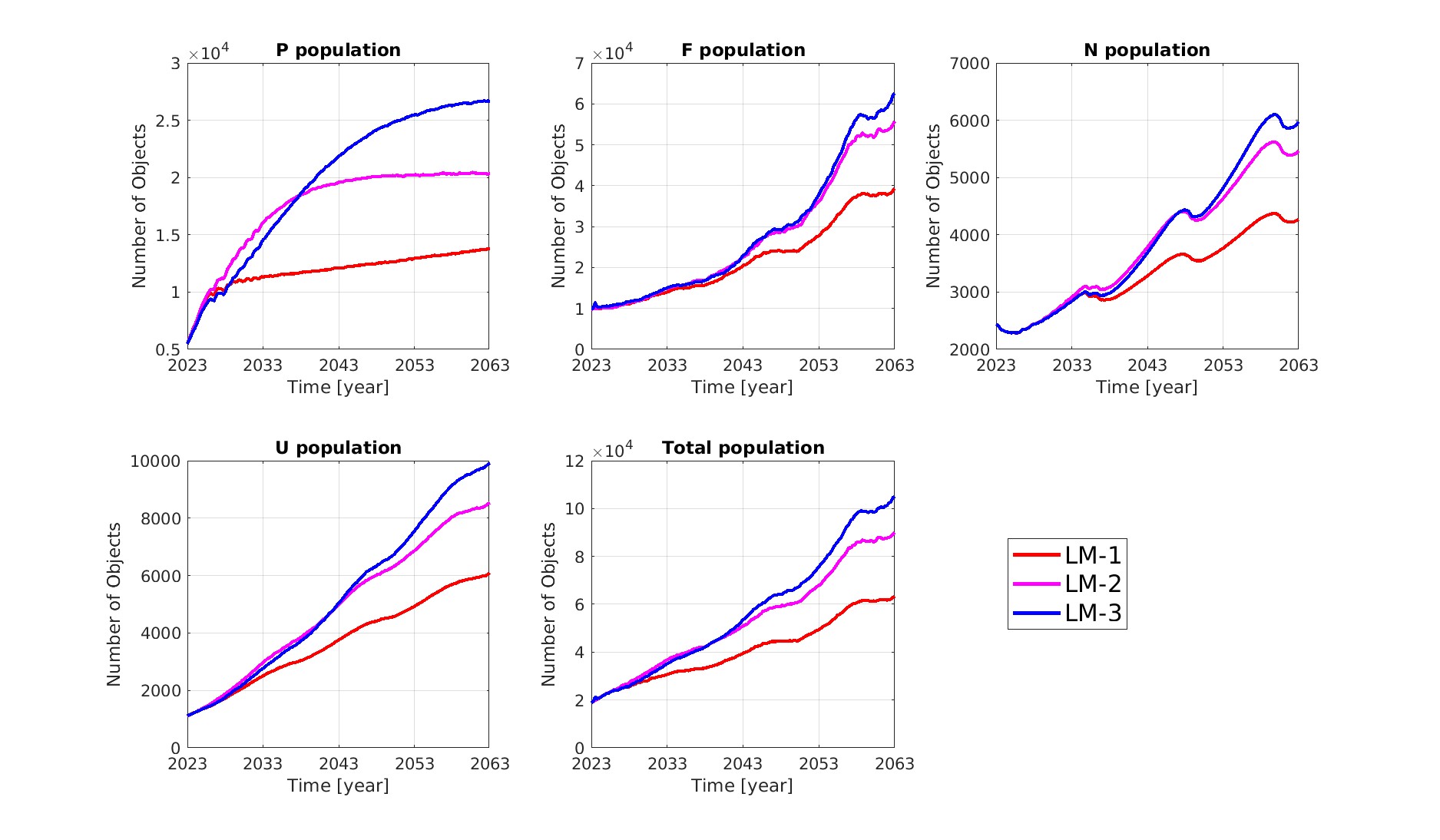
Figure 14: Mean evolution of different species for 3 different launch models.

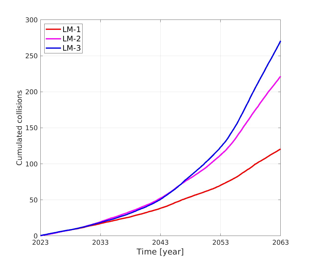
Figure 15: Mean cumulative number of collisions for 3 different launch models.

4.2 Impacts of Debris Mitigation Actions

This section investigates the impact of debris mitigation actions, such as the success rate of collision avoidance maneuvers (CAM) and the failure rate of post-mission disposal (PMD), on the space environment.

On the one hand, considering $s_{CAM}$ values of 0%, 10%, 40%, 70%, and 90% with fixed $\gamma=5\%$, Figure 16 compares the temporal evolution of each species under launch traffic model #1. Overall, simulation results suggest that an decrease in $s_{CAM}$ results in an increase in final population and cumulated collisions. Compared to Figure 14 and Figure 15, decreasing $s_{CAM}$ from $99.99\%$ to $0\%$ results in an increase in final population of fragments from around 39,000 to around 82,000, and an increase in cumulated collisions from 120 to 500. Specifically, as $s_{CAM}$ decreases, the probability of collision between payloads and other objects increase, leading to a reduction in the number of upper stages and an increase in fragments. Interestingly, the number of non-maneuverable satellites shows a slight increase as $s_{CAM}$ decreases. This is because the additional fragments generated by payloads-related collisions further increase the probability of small collisions, that is, the increased likelihood that payloads will be converted in non-maneuverable satellites due to the increase in the number of small fragments between 1 cm and 10 cm. Moreover, the stronger oscillation behavior observed in fragments counts at lower $s_{CAM}$ further proved that the additional fragments originate from payloads-related collisions. A lower $s_{CAM}$ results in more fragments with a higher area-to-mass ratio, as they are generated from payload-related collisions. The higher area-to-mass ratio makes these fragments more susceptible to atmospheric drag, leading to stronger oscillations in fragment numbers over time.

On the other hand, considering $\gamma$ values of 0%, 10%, 20%, 30% and 40%, Figure 17 compares the temporal evolution each species under launch traffic model #1. Overall, simulation results suggest that an increase in $\gamma$ results in an increase in final population and cumulated collisions. Compared to Figure 14 and Figure 15, increasing $\gamma$ from $5\%$ to $40\%$ results in an increase in final population of fragments from around 39,000 to around 64,000, and an increase in cumulated collisions from 120 to 265. Specifically, as $\gamma$ increase, more payloads fail to perform post-mission disposal, resulting in an increase of non-maneuverable satellites, and thereby an increase in fragments. Notably, $\gamma=0\%$ results in a decrease trend of non-maneuverable satellites, while other values results in increase trends of non-maneuverable satellites. Consistent with the aforementioned conclusions, a stronger oscillation behavior of fragments resulted from higher $\gamma$ indicates that new fragments have higher area to mass ratio. Although these new fragments are not directly generated from payloads, they mostly result from collisions related to non-maneuverable satellites, where the majority of non-maneuverable satellites originate from payloads that failed to implement post-mission disposal.

In summary, the simulation results suggest that increasing satellite maneuverability, either by increasing $s_{CAM}$ or decreasing $\gamma$, leads to a lower final population. However, this does not stop the overall increasing trend of fragments. In other words, while the mitigation actions help delay the deterioration of the space environment, they cannot fully prevent it. This aligns with conclusions from previous studies [22], which suggests that the mitigation measures will restrict the growth, but it is unlikely to stop the long-term debris population in LEO from increasing. Consequently, these results have led to the consideration of Active Debris Removal (ADR) as a necessary measure to remediate the space environment.

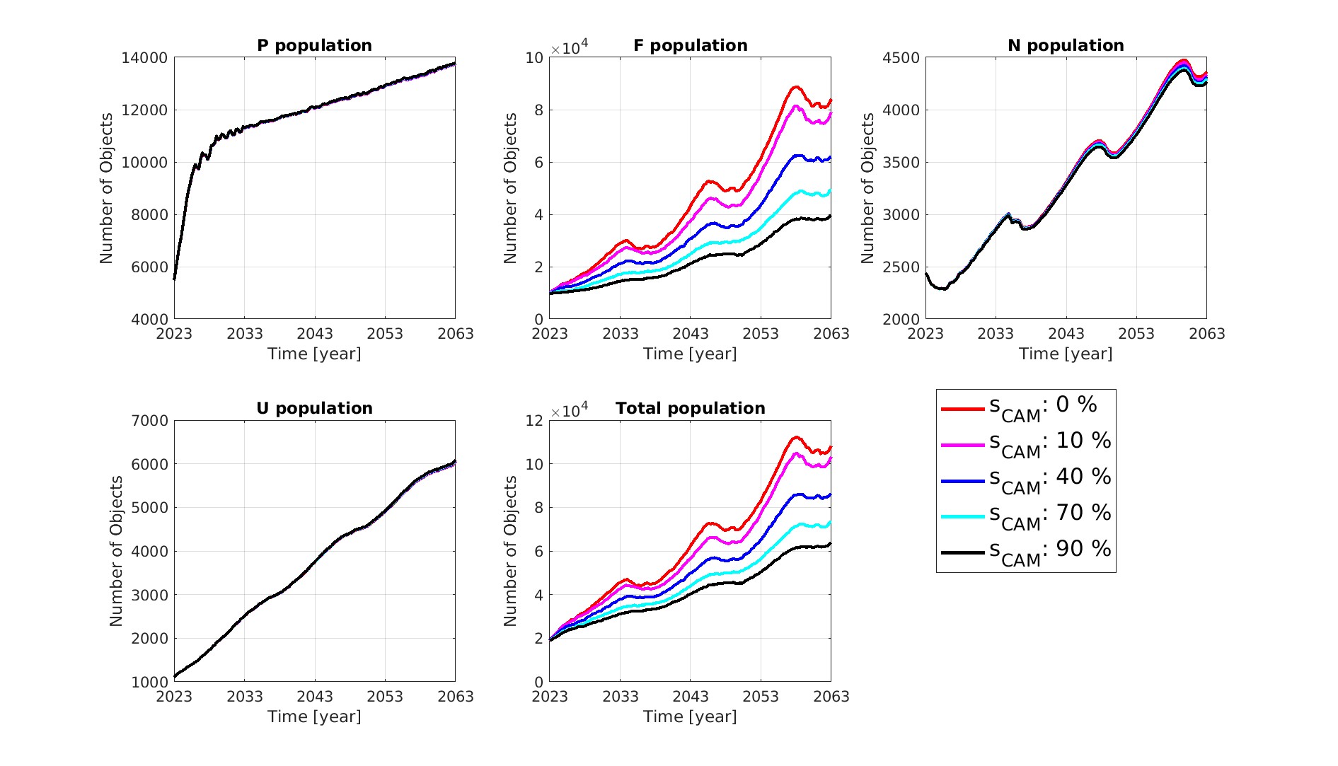
Figure 16: Impact of $s_{CAM}$ on the population evolution.

.

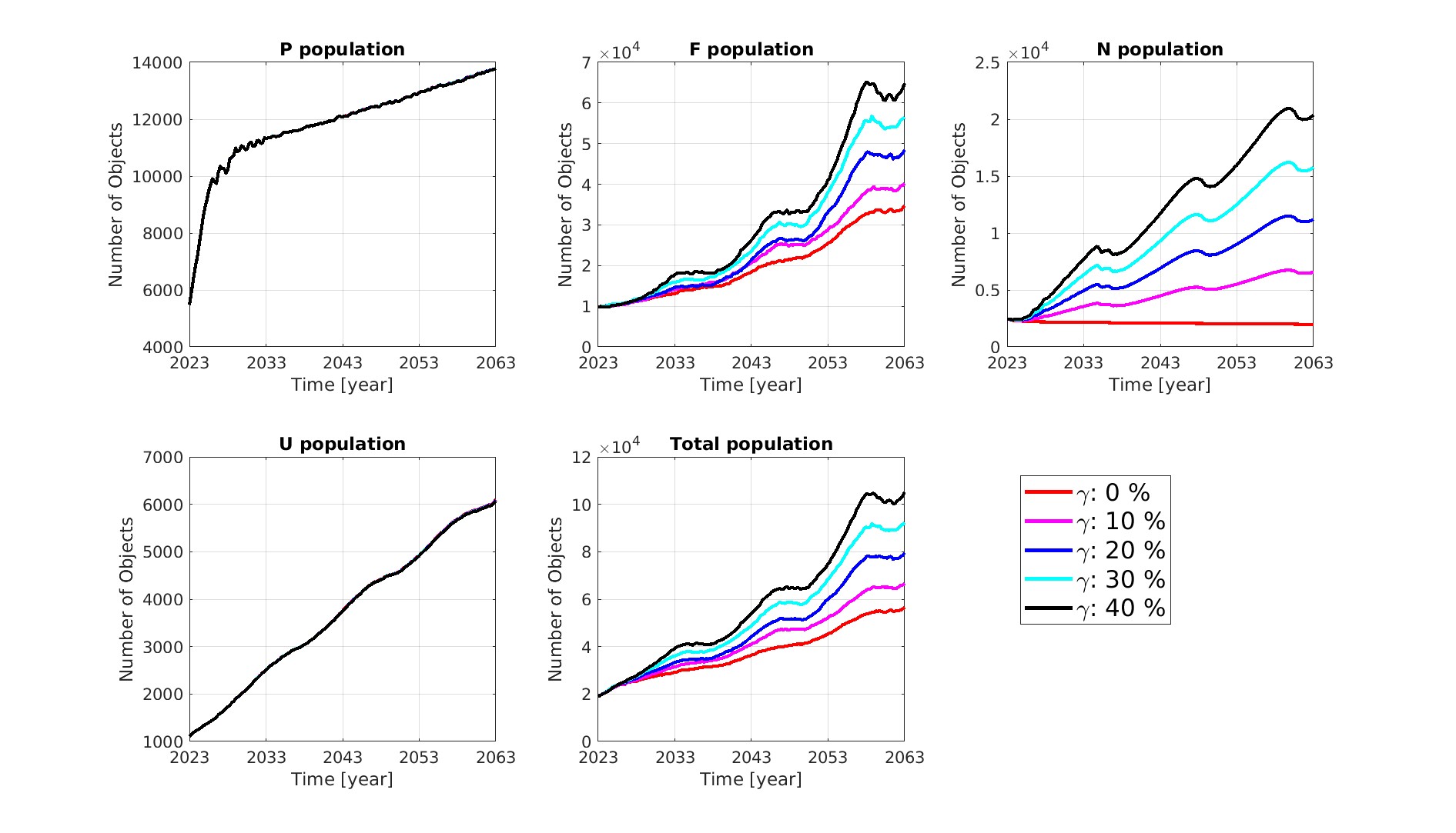
Figure 17: Impact of $\gamma$ on the population evolution.

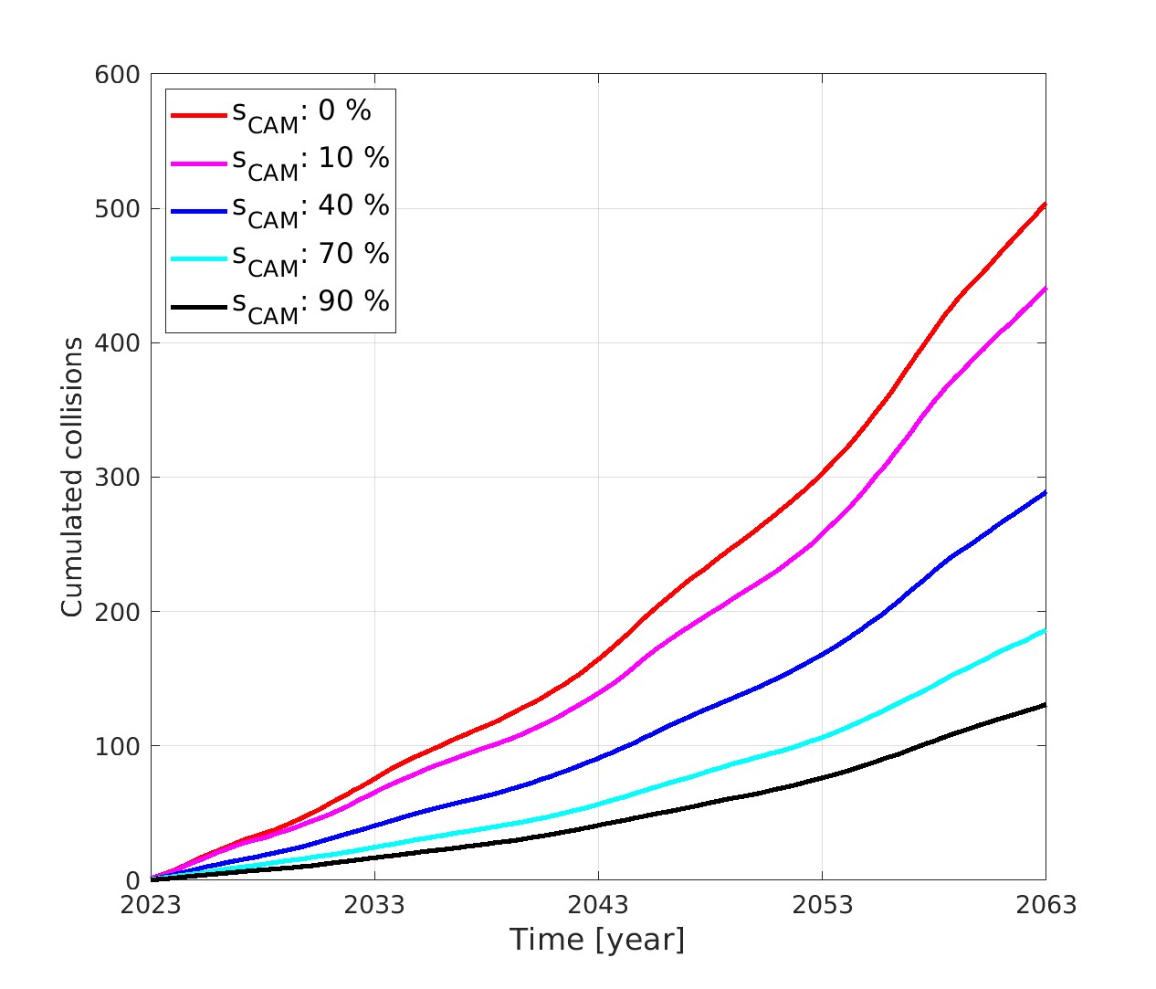
Figure 18: Impact of $s_{CAM}$ on the number of collisions

.

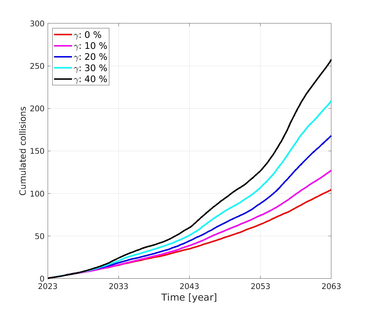
Figure 19: Impact of $\gamma$ on the number of collisions.

5 Topological and Dynamical Properties of the Network

The topological properties of a network are exclusively determined by the number of nodes and their connections, while the dynamical properties are defined by the dynamic evolution of links and nodes. Both properties can be studies by analyzing an adjacency matrix derived from the evolutionary equations in Eq.(1), which encapsulates the connection probability among nodes. This section begins with the definition of the network links, followed by the centrality analysis of the network.

5.1 Definition of the Network Links

Each node $S_{i}$ is multi-connected to other nodes $S_{j}$ in the network. Hence, one can compute the probability that each of the connections exists within a given time $\Delta t_{k}$. Connection probabilities include: i) the probability of a collision between node $S_{i}$ and node $S_{j}$, denoted by $p^{\mathcal{C}}_{S_{i}S_{j}}$, ii) the probability of the fragments generated from node $S_{i}$ flowing to node $S_{j}$, denoted by $p^{\mathcal{F},F}_{S_{i}S_{j}}$, iii) the probability of objects flowing from node $S_{i}$ to node $S_{j}$ due to the natural decay, denoted by $p^{\mathcal{F},D}$, and iv) the probability of objects flowing from node $S_{i}$ to node $S_{j}$, due to the PMD failure, denoted by $p^{\mathcal{F},PMD}_{S_{i}S_{j}}$. The probability $p_{S_{i}S_{j}}$ that at least one link exists, is, therefore, defined by:

$$p_{S_{i}S_{j}}=\max\{p^{\mathcal{C}}_{S_{i}S_{j}},p^{\mathcal{F},F}_{S_{i}S_{j}},p^{\mathcal{F},D}_{S_{i}S_{j}},p^{\mathcal{F},PMD}_{S_{i}S_{j}}\}$$ (23)

The probability $p_{S_{i}S_{j}}$ is a function of the connection rate $\chi_{S_{i}S_{j}}$, according to [11]:

$$p_{S_{i}S_{j}}=1-e^{-\chi_{{S_{i}}{S_{j}}}\Delta t_{k}}$$ (24)

and the connection rate $\chi_{S_{i}S_{j}}$ for different types of connections is defined as:

$$\begin{cases}\chi^{\mathcal{C}}_{S_{i}S_{j}}=\tau^{*}_{S_{i}S_{j}}\\ \chi^{\mathcal{F},F}_{S_{i}S_{j}}=\sum_{S_{l}\in\mathcal{S}}\sum^{n}_{l=1}\tau^{*}_{S_{i}S_{l}}\xi^{S_{j}}_{S_{i}S_{l}}\\ \chi^{\mathcal{F},D}_{S_{i}S_{j}}=\frac{\varepsilon_{S_{i}S_{j}}}{\Delta t_{k}}\\ \chi_{S_{i},S_{j}}^{\mathcal{F},PMD}=\Delta S_{i}^{\gamma}\quad\text{if }(i=j)\land(S_{i}=P_{i})\land(S_{j}=N_{j})\end{cases}$$ (25)

where $\mathcal{S}=\{P,U,N,F\}$ and $\tau^{*}_{{S_{i}}{S_{j}}}$ indicates the effective collision rate with the consideration of both $s_{CAM}$ and $\kappa$. For example, from the first equation in system Eq.(1) one can see that the collision rate between payloads node $P_{i}$ and fragments node $F_{j}$ has to be scaled by $1-s_{CAM}$ and has to account for small collisions factor. Thus, in this case, the effective collision rate is

$$\tau^{*}_{P_{i}F_{j}}=(1-s_{CAM}+\kappa)\tau_{P_{i}F_{j}}$$ (26)

The quantity $\xi^{S_{j}}_{S_{i}S_{l}}$ indicates the fraction of fragments flowing from node $S_{i}$ to node $S_{j}$ after the collision between node $S_{i}$ and node $S_{l}$:

$$\xi^{S_{j}}_{S_{i}S_{l}}=\frac{\zeta^{S_{j}}_{S_{i}S_{l}}}{\zeta_{S_{i}S_{l}}}$$ (27)

where $\zeta_{S_{i}S_{l}}$ indicates the total amount of fragments generated from the collision between node $S_{i}$ and node $S_{l}$. Given that $\xi^{S_{j}}_{S_{i}S_{l}}$ from a catastrophic collision can be estimated by a constant once the species and orbital region are fixed, $\xi^{S_{j}}_{S_{i}S_{l}}$ can be pre-calculated to save the computational time. Assuming that there are two massive objects, with the mass of 20,000 kg for each, from node $S_{i}$ and node $S_{j}$ collide with each other within their respective orbital regions, the redistribution of new fragments is determined by NASA’s breakup model and the network configuration. This redistribution process is repeated 10 times to obtain the average $\zeta^{S_{j}}_{S_{i}S_{l}}$ for each pair of nodes. These average values are stored in a pre-calculated tensor $\mathbf{T}$ with the corresponding element $T_{ilj}$. Quantity $\Delta^{\gamma}_{S_{i}}$ represents the amount of objects flowing from node $S_{i}$ to node $S_{j}$ due to the PMD failure and $\varepsilon_{S_{i}S_{j}}$ represents the amount of objects flowing from node $S_{i}$ to node $S_{j}$ due to the orbital decay, where $\varepsilon_{S_{i}S_{j}}$ is non-zero only if node $S_{i}$ and node $S_{j}$ are the same species and $j=i-1$.

5.2 Centrality Analysis of the Network

In network analysis, in-degree and out-degree are key metrics used to describe the centrality of nodes within a directed graph. In-degree refers to the number of incoming connections that a node receives from other nodes, representing the extent to which a node is influenced by others in the network. A higher in-degree indicates that a node is central within the network, receiving more interactions. On the other hand, out-degree measures the number of outgoing connections that a node sends to other nodes. It reflects the level of influence of a node in terms of initiating interactions with others. Nodes with a high out-degree are typically more actively playing a critical role in diffusing the effects of an event across the network. The critical nodes can be identified according to their centrality.

Define subnetwork $G_{\rho}$, where nodes $S_{i}$ and $S_{j}$ are connected if $p_{S_{i}S_{j}}\geq\rho$. Figure 20 shows the in-degree distribution of different subnetworks $G_{\rho}$ with $\rho$ = 0, 1e-6, 1e-3, 1e-1 at the snapshot of year 2023, where the network is represented in a lattice structure, while Figure 21 shows the distribution of out-degree under the same conditions. These figures provide a first indication of nodes centrality. Overall, as $\rho$ increases, less and less links exist in the subnetworks, and the nodes show different criticality in each subnetwork $G_{\rho}$. For instance, $\rho=0$ represents a subnetwork with all the non-zero links, and it suggests that $F$ nodes with the altitude range of [1000, 1100] km and the inclination range of $[0,60]^{\circ}$ show the highest in-degree, suggesting that these nodes act as strong sinks to attract fragments generated from collision events. On the other hand, the $U$ nodes in the altitude range of [1000, 1200] km and the inclination bin $[60,120]^{\circ}$ show the highest out-degree, indicating that they are the most hazardous objects for spreading debris to other nodes in the network. However, the node with the highest in-degree/out-degree changes over $\rho$. For example, while a $U$ node has the highest out-degree in the subnetwork $G_{\rho=0}$, the associated link weights are relatively weak. As observed in the subnetwork $G_{\rho=1e-3}$, a $F$ node becomes the one with the highest out-degree. These observations highlight the need of considering both the direction and the weight of the links when conducting centrality analysis. Therefore, the weighted in-degree $\hat{d}_{in}$ and weighted out-degree $\hat{d}_{out}$ are used to evaluate the importance of each node which considers both direction and weight of each link

$$\begin{cases}\hat{d}_{in}(S_{i})=\sum_{S_{j}\in\mathcal{S}}\sum^{n}_{j=1}p_{S_{j}S_{i}}\\ \hat{d}_{out}(S_{i})=\sum_{S_{j}\in\mathcal{S}}\sum^{n}_{j=1}p_{S_{i}S_{j}}\end{cases}$$ (28)

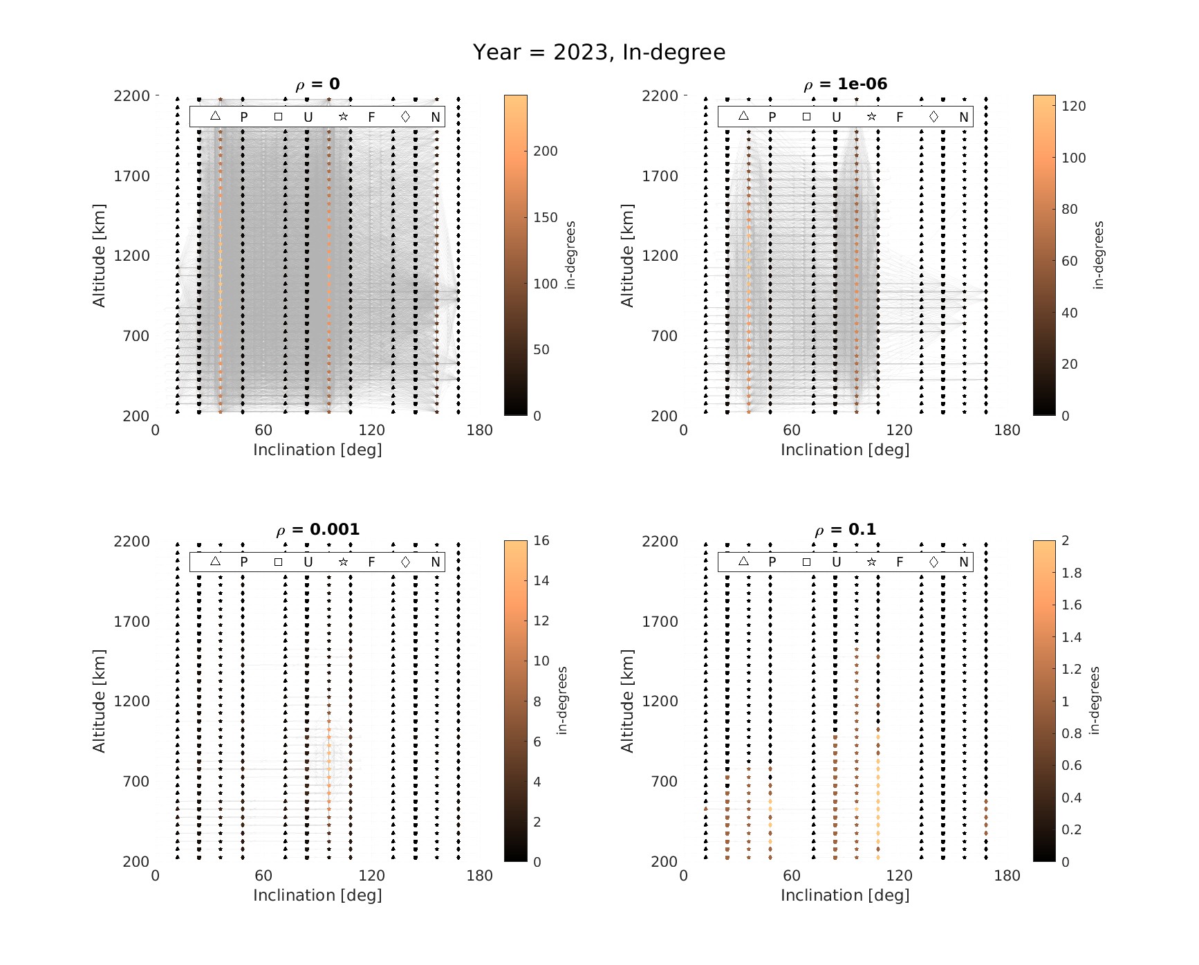
Figure 20: Representation of the network of nodes with the lattice structure at year 2023 (In-degree).

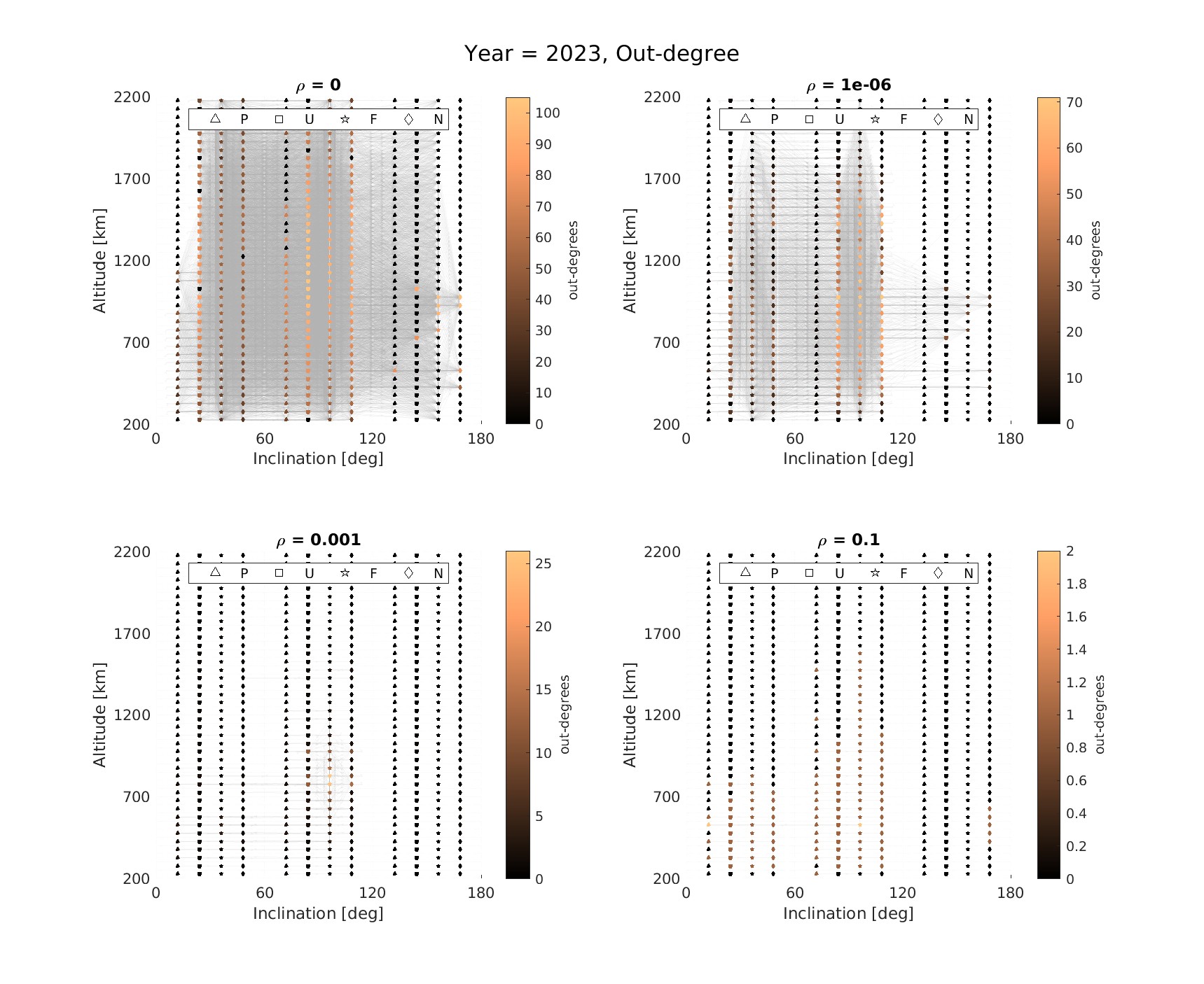
Figure 21: Representation of the network of nodes with the lattice structure at year 2023 (Out- degree).

Table 4 presents a comprehensive summary of the top 5 nodes with highest centrality values for the Baseline case of year 2023, 2063 and 2103. Specifically, at year 2023, node 114, representing a group of non-maneuverable satellites located at the orbital regime with orbital shell $h\in[550,600]$ km and inclination $i\in[60,120]^{\circ}$, appears to be most susceptible due to the failure PMD of payloads and decay of the non-maneuverable satellites from a higher orbital shell. Given 5-year life time of the payloads, during the initial years, the $N$ nodes appears to be affected by the $P$ nodes due to the failure PMD. A group of fragments located at the orbital shell $h\in[500,550]$ km and inclination $i\in[60,120]^{\circ}$ appear to be most dangerous objects for spreading fragments to the rest of nodes in the network. Moreover, there are same top 5 nodes ranked in year 2063 and 2103 with the similar centrality values. suggesting that the self-connections of these nodes play a critical role, which means those with significant self-collisions risks are becoming the critical nodes over years in the Baseline case. Those nodes identified with both highest in-degree and out-degree appear to grow fast due to the self collisions.

Table 5 presents a comprehensive summary of the top 5 nodes with highest centrality values for the new launches scenario of year 2023, 2063, and 2103. Compared to the baseline scenario, the centrality values of the top 5 nodes in the new launch case increase over time. Additionally, the critical nodes identified for 2063 and 2103 differs from the Baseline case, which are not limited to the $F$ nodes but also include $P$, $N$, and $U$ nodes. For instance, in both year 2063 and year 2103, node 113, which is an $F$ node located in the orbital shell $h\in[550,600]$ km with an inclination of $i\in[60,120]^{\circ}$, is identified as the most critical node in terms of both in-degree and out-degree, and its centrality values of both in-degree and out-degree increased in 2103 compared to 2063. It can be seen that for the other 4 nodes also located in the similar region, indicating that the increased congestion resulting from launch traffic causes nodes in those congested region to become more critical. Basically, as shown in the identification results, in the congested region, apart from the $F$ nodes, the $N$ nodes appear to be identified as the strongest sink to be affected by other nodes, and $P$ and $U$ nodes appear to be identified as the strongest source to affect other nodes.

Table 4: Top 5 nodes of centrality measures based on the snapshots of 2023, 2063 and 2103, Baseline case.

Snapshot	Centrality	Top nodes			Objects number	Location				Class
		rank	node ID	Centrality value		height bin [km]		inclination bin [deg]
2023	in-degree	1	114	1.99	131	550	600	60	120	’N’
		2	84	1.93	95	450	500	60	120	’N’
		3	99	1.80	73	500	550	60	120	’N’
		4	69	1.65	71	400	450	60	120	’N’
		5	98	1.54	183	500	550	60	120	’F’
	out-degree	1	98	1.52	183	500	550	60	120	’F’
		2	173	1.19	1072	750	800	60	120	’F’
		3	188	1.16	1311	800	850	60	120	’F’
		4	113	1.10	310	550	600	60	120	’F’
		5	111	1.07	375	550	600	60	120	’P’
2063	in-degree	1	173	1.12	1831	750	800	60	120	’F’
		2	188	1.12	2072	800	850	60	120	’F’
		3	203	1.09	1945	850	900	60	120	’F’
		4	233	1.08	1201	950	1000	60	120	’F’
		5	158	1.08	1990	700	750	60	120	’F’
	out-degree	1	173	1.16	1831	750	800	60	120	’F’
		2	188	1.15	2072	800	850	60	120	’F’
		3	233	1.09	1201	950	1000	60	120	’F’
		4	203	1.08	1945	850	900	60	120	’F’
		5	158	1.08	1990	700	750	60	120	’F’
2103	in-degree	1	188	1.11	2409	800	850	60	120	’F’
		2	173	1.11	2036	750	800	60	120	’F’
		3	233	1.09	1368	950	1000	60	120	’F’
		4	203	1.08	2008	850	900	60	120	’F’
		5	218	1.07	1787	900	950	60	120	’F’
	out-degree	1	173	1.16	2036	750	800	60	120	’F’
		2	188	1.14	2409	800	850	60	120	’F’
		3	233	1.10	1368	950	1000	60	120	’F’
		4	158	1.07	1629	700	750	60	120	’F’
		5	203	1.07	2008	850	900	60	120	’F’

Table 5: Top 5 nodes of centrality measures based on the snapshots of 2023, 2063 and 2103, with new launches.

Snapshot	Centrality	Top nodes			Objects number	Location				Class
		rank	node ID	Centrality value		height bin [km]		inclination bin [deg]
2023	in-degree	1	114	1.99	111	550	600	60	120	’N’
		2	84	1.94	101	450	500	60	120	’N’
		3	99	1.78	70	500	550	60	120	’N’
		4	69	1.67	65	400	450	60	120	’N’
		5	98	1.54	188	500	550	60	120	’F’
	out-degree	1	98	1.52	188	500	550	60	120	’F’
		2	173	1.18	1022	750	800	60	120	’F’
		3	188	1.17	1350	800	850	60	120	’F’
		4	113	1.10	295	550	600	60	120	’F’
		5	91	1.08	2953	500	550	0	60	’P’
2063	in-degree	1	113	3.31	4621	550	600	60	120	’F’
		2	98	2.48	1556	500	550	60	120	’F’
		3	94	2.22	437	500	550	0	60	’N’
		4	99	2.10	730	500	550	60	120	’N’
		5	84	2.03	263	450	500	60	120	’N’
	out-degree	1	113	3.46	4621	550	600	60	120	’F’
		2	98	2.39	1556	500	550	60	120	’F’
		3	111	2.07	2857	550	600	60	120	’P’
		4	106	1.91	1806	550	600	0	60	’P’
		5	96	1.89	3835	500	550	60	120	’P’
2103	in-degree	1	113	4.99	8336	550	600	60	120	’F’
		2	98	4.55	4984	500	550	60	120	’F’
		3	108	4.16	4356	550	600	0	60	’F’
		4	128	3.84	14533	600	650	60	120	’F’
		5	93	3.63	2448	500	550	0	60	’F’
	out-degree	1	113	5.21	8336	550	600	60	120	’F’
		2	108	5.06	4356	550	600	0	60	’F’
		3	128	4.55	14533	600	650	60	120	’F’
		4	112	4.38	1396	550	600	60	120	’U’
		5	98	4.27	4984	500	550	60	120	’F’

6 Space Carrying Capacity and Network Dynamics

In this section we study the relationship between network dynamics and the concept of space carrying capacity. The idea of looking for equilibrium points was already introduced in previous works, see [39] or [9]. Here we apply the same idea to the network dynamics.

6.1 Carrying capacity of one-dimensional network dynamics

In ecological networks the carrying capacity of an environment in relation to the population $x$ living in that environment and the available resources is expressed by the Verhulst model:

$$\dot{x}=rx-\frac{r}{K}x^{2}$$ (29)

where $r$ is the birth rate minus the death rate of the population and $K$ is the carrying capacity of the environment. Eq. (29) has two equilibrium points: $x=0$ and $x=K$. Hence the carrying capacity is an equilibrium of the population dynamics. In the case of the Verhulst model, it is easy to see that $x=K$ is stable, hence if the population is higher than $K$, it reduces to $K$ and if it is lower than $K$, it grows till reaching $K$.

In analogy with model (29) we can consider the case in which asymptotically, in the case of no new launches, the space environment is occupied only by a single species, the fragments. The mean evolution of the fragments can be written as:

$$\dot{x}=-ax+bx^{2}$$ (30)

where $a$ is the rate of decay per unit time and object and $b$ is the production of debris per unit time and object square. If the cross section area of the objects remains constant and the decay is not dependent on the Sun cycle, then $a/b$ is a constant. In this case, Eq. (30) has two equilibrium points, $x=0$ and $x=a/b$, where $x=0$ is stable and $x=a/b$ is unstable. More specifically for $x>a/b$ the environment diverges to infinity and for $x<a/b$ it converges to 0. In fact, (30) is a Bernulli equation with solution:

$$x(t)=\frac{e^{-at}}{b\frac{e^{-at}}{a}+C_{0}}$$ (31)

which has a vertical asymptote for $b\frac{e^{-at}}{a}+C_{0}=0$ if $x(0)>b/a$. We can, therefore, define $a/b$ has the carrying capacity since above this value the environment diverges to infinity.

We tested this simple one-dimensional model by propagating the environment with NESSY, assuming that only one species, the fragments, was present. We derive the coefficients $a$ and $b$ from Eq. (1) as follows:

$$\begin{cases}a=\frac{\mathbb{E}(\Delta x_{decay})}{x\Delta t}\\ b=\frac{\mathbb{E}(\Delta x^{FF}_{collision})}{x^{2}\Delta t}\end{cases}$$ (32)

where $\mathbb{E}(\Delta x_{decay})$ indicates the expected change in fragments due to the atmospheric drag

$$\mathbb{E}(\Delta x_{decay})=\sum^{n}_{i=1}\left(x_{i}-(\varepsilon^{+}_{F_{i}}-\varepsilon^{-}_{F_{i}})\right)$$ (33)

and $\mathbb{E}(\Delta x^{FF}_{collision})$ indicates the expected change in fragments due to the self-collisions

$$\mathbb{E}(\Delta x^{FF}_{collision})=\sum_{i}\left(-\sum_{j}\tau_{F_{i}F_{j}}\Delta t_{k}+\sum_{j}\sum_{l}\Delta_{F_{j}F_{l}}\zeta^{F_{i}}_{F_{j}F_{l}}\Delta t_{k}\right)$$ (34)

Given that different populations $x$ might results in different coefficients, due to the distribution of cross-section areas, and coefficients are not constant over time, here we take an average across multiple initial populations and an average over the propagation time. In Table 6 the populations chosen for the test cases presented, propagated with both NESSY and analytical equations.

Table 6: Initial populations test cases for carrying capacity analysis.

Test case	$\#$ fragments	$\#$ payloads
Baseline	9804	5771
Test 1	49020	13942
Test 2	68628	13942
Test 3	98040	19413

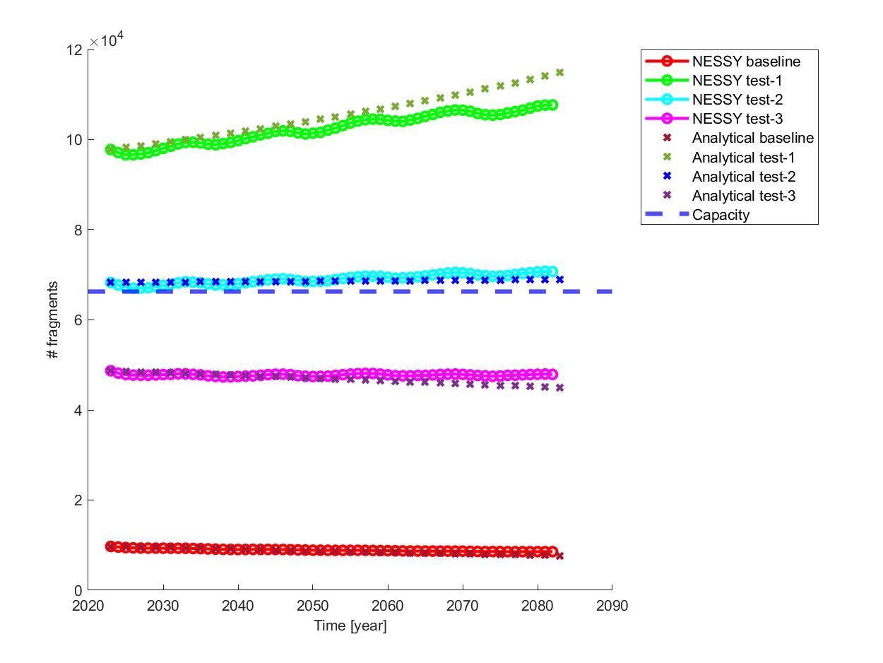
Figure 22: Carrying capacity analysis just with fragments population (test cases defined in Table 6).

Figure 22 shows the result of the environment propagation with NESSY (dotted lines) for the different initial conditions, considering just one node for the network. Note that the capacity is here the mean value over several Sun cycles. It is clear that when the initial population is higher than the capacity (horizontal dashed line) the population diverges, while if it is initially lower it tends to zero, as expected. The propagation with NESSY was performed with a 1-year time step for 60 years and considering 30 independent runs to compute the mean trend. The capacity is computed with respect to the baseline case, which corresponds to the actual population in 2023, averaging the coefficients about the random runs and time. The NESSY propagation is compared with the propagation performed with the analytical equations shown before (represented with crosses in the plot).

One can now ask which other equilibrium points the network dynamics has. In this paper, we limit our investigations to a simple mean-field case with two nodes representing the fragments and all new objects launched into space. More complex analyses over the whole network are deferred to future studies. Note that this case, although simple, is representative of a range of realistic situations as it will be explained in the remainder of this section.

6.2 Carrying capacity of two-dimensional network dynamics

If one considers only fragments $x$ and payloads with new launches $y$, the evolutionary equations simplify to:

$$\begin{array}[]{l}\dot{x}=bx^{2}-ax+cy^{2}+dxy\\ \dot{y}=-ey^{2}-fxy+\lambda-\gamma y\end{array}$$ (35)

Coefficient $a$ is the rate of fragments decay per unit time and object, $b$ is the rate of generation of fragments per unit time and fragment squared, $c$ is the rate of generation of fragments per unit time and payload squared, $d$ is the rate of fragment generation per unit time and object squared due to collisions between fragments and payloads, $e$ is the number of collisions between payloads per unit time and payload squared, $f$ is the number of collisions between payloads and fragments per unit time and object squared. The other two coefficients are $\lambda$, which is considered for the following simulations 3000 payloads launched per year, and $\gamma$, which is instead computed as the rate of post-mission disposals per unit objects. No small collision collision, $\kappa=0$, is considered in this case. The equilibrium points are found by solving:

$$\begin{array}[]{l}bx^{2}-ax+cy^{2}+dxy=0\\ -ey^{2}-fxy+\lambda-\gamma y=0\end{array}$$ (36)

where the value of the coefficients is:

$$\begin{cases}a=\frac{\mathbb{E}(\Delta x_{decay})}{x\Delta t}\\ b=\frac{\mathbb{E}(\Delta x^{FF}_{collision})}{x^{2}\Delta t}\\ c=\frac{\mathbb{E}(\Delta x^{PP}_{collision})}{y^{2}\Delta t}\\ d=\frac{\mathbb{E}(\Delta x^{PF}_{collision})}{xy\Delta t}\\ e=\frac{\mathbb{E}(\Delta y^{PP}_{collision})}{y^{2}\Delta t}\\ f=\frac{\mathbb{E}(\Delta y^{PF}_{collision})}{xy\Delta t}\\ \gamma=\frac{\mathbb{E}(y_{PMD})}{y\Delta t}\end{cases}$$ (37)

The expected values $\mathbb{E}(x_{decay})$ and $\mathbb{E}(\Delta x^{FF}_{collision})$ have the same meaning as in Eq.(33) and Eq.(34) under the assumption that there is no decay of payloads due to atmospheric drag. Quantity $\mathbb{E}(\Delta x^{PP}_{collision})$ indicates the expected change in fragments due to the self-collisions of payloads.

$$\mathbb{E}(\Delta x^{PP}_{collision})=\sum_{i}\left(-\sum_{j}(1-s_{CAM})^{2}\tau_{P_{i}P_{j}}\Delta t_{k}+\sum_{j}\sum_{l}\Delta_{P_{j}P_{l}}\zeta^{F_{i}}_{P_{j}P_{l}}\Delta t_{k}\right)$$ (38)

$\mathbb{E}(x^{PF}_{collision})$ indicates the expected change in fragments due to the collisions between payloads and fragments.

$$\mathbb{E}(\Delta x^{PF}_{collision})=\sum_{i}\left(-\sum_{j}(1-s_{CAM})\tau_{P_{i}F_{j}}\Delta t_{k}+\sum_{j}\sum_{l}\Delta_{P_{j}P_{l}}\zeta^{F_{i}}_{P_{j}P_{l}}\Delta t_{k}\right)$$ (39)

$\mathbb{E}(\Delta y^{PP}_{collision})$ indicates the expected change in payloads due to the self-collisions of payloads

$$\mathbb{E}(\Delta y^{PP}_{collision})=\sum_{i}\left(-\sum_{j}(1-s_{CAM})^{2}\tau_{P_{i}P_{j}}\Delta t_{k}\right)$$ (40)

$\mathbb{E}(\Delta y^{PP}_{collision})$ indicates the expected change in payloads due to the collisions between payloads and fragments.

$$\mathbb{E}(\Delta y^{PF}_{collision})=\sum_{i}\left(-\sum_{j}(1-s_{CAM})\tau_{P_{i}F_{j}}\Delta t_{k}\Delta t_{k}\right)$$ (41)

Quantity $\mathbb{E}(y_{PMD})$ indicates the expected change in payloads due to PMD. Similar to the one-dimensional case, we take an average across multiple initial populations and an average over the propagation time, for each coefficient.

NESSY was run again from the initial populations in Table 6: the baseline is without new launches, while the other three cases include new launches, considering just payloads and fragments. Table 7 reports the settings used to run NESSY on these cases.

Table 7: NESSY mission-related parameters.

$s_{CAM}$	$\gamma$	Payload Mission lifetime	$\kappa$
99.99$\%$	0 $\%$	5 years	0

Each initial population was propagated for 60 years with a one year time step, and each run was repeated for 30 times to compute the average variation of each species. The network is composed of only one node for each species. The results of the propagations are presented in Fig.25 to Fig.28. Figures 24, 26 and 28 show the time evolution of the coefficients of Eqs. (35) derived from NESSY. Fig. 23, 25 and 27 show the evolution of the two species computed with NESSY and compared to the propagation of Eqs. (35). The level curves represent the value of $\sqrt{\dot{x}^{2}+\dot{y}^{2}}$. The equilibrium points were initially identified by finding the minima of $\sqrt{\dot{x}^{2}+\dot{y}^{2}}$ with the MatLab fminunc function.

For a zero launch rate, one equilibrium solution is $[0,0]$ while the other is $[a/b,0]$. From the Jacobian matrix, one can see that $[0,0]$ is linearly stable because the Jacobian has two real negative eigenvalues, while for $[a/b,0]$, it has one negative and one positive real eigenvalue. Hence, there is a stable manifold that brings the space environment towards $[a/b,0]$ and an unstable manifold that diverges from $[a/b,0]$ and either connects to the stable manifold of $[0,0]$ or diverges to infinity. Figure 23 shows the existence of these two equilibrium solutions. The propagation of system (35) (indicated with an ”x” symbol in Fig.23), with the average of the coefficients in Figure 24), shows the expected convergence to the stable point and the stable manifold along the y axis. The propagation with NESSY (continuous lines with circle markers) follows the same trend, confirming the theory.

For a non-zero launch rate, we can distinguish two extreme cases: a) all new launches are manoeuverable and can avoid collisions with 99.99% probability or b) all new launches are non-manoeuverable and can collide among each other and with fragments. In the former case, system (35) still has two equilibrium solutions: $[\epsilon,y_{eq}]$ and $[k,y_{eq}]$. Where again $[\epsilon,y_{eq}]$ is stable and $[k,y_{eq}]$ is unstable with one stable manifold and one unstable manifold. The value $\epsilon$ is small for high collision avoidance rate and goes to zero when collision avoidance is 100%. Figure 25 shows the case with manoeuverable payloads. The corresponding time history of the coefficients can be found in Figure 26. Coefficient $a$ follows the variation of atmospheric density as expected, while $b$ progressively reduces due to the decay of fragments and the reduction in cross section area of the fragments. It is important to remark that in this example there are no collisions between lethal non-trackable fragments and other objects or fragments.

Continuous lines with circle markers in Figure 25 represent the propagation with NESSY while the propagation of system (35) is represented by the ”x” marker. In this case one can see two distinct equilibrium points for a non-zero value of $y$, one stable and one unstable. Note that when the simulations with NESSY start above $y_{eq}$, $y$ initially grows and then converges to the equilibrium value. This initial growth, observed only in the early years, is attributed to resident payloads. Most of these payloads are not removed by PMD because they remain within their operational lifetimes.

Figure 27 shows the case with non-maneouverable payloads. The time history of the coefficients is in Figure 28. In this case there is no equilibrium solution for the fragments, while the payloads converge to a stable equilibrium.

Hence, we can say that the capacity of the environment to host new objects is given by the region of the $[x,y]$ space in between the two stable manifolds respectively of $[\epsilon,y_{eq}]$ and $[k,y_{eq}]$. When the two points collapse, there is zero capacity. In general, if the removal rate, given by a combination of PMD and decay, plus the collision avoidance rate are higher than the generation of new fragments, the system presents two distinct equilibria.

The values of the coefficients and respective equilibria are reported in Table 8. Note that for the case with 0% $s_{CAM}$ we report only the equilibrium value for $\dot{y}=0$ since there is no equilibrium $\dot{x}=0$.

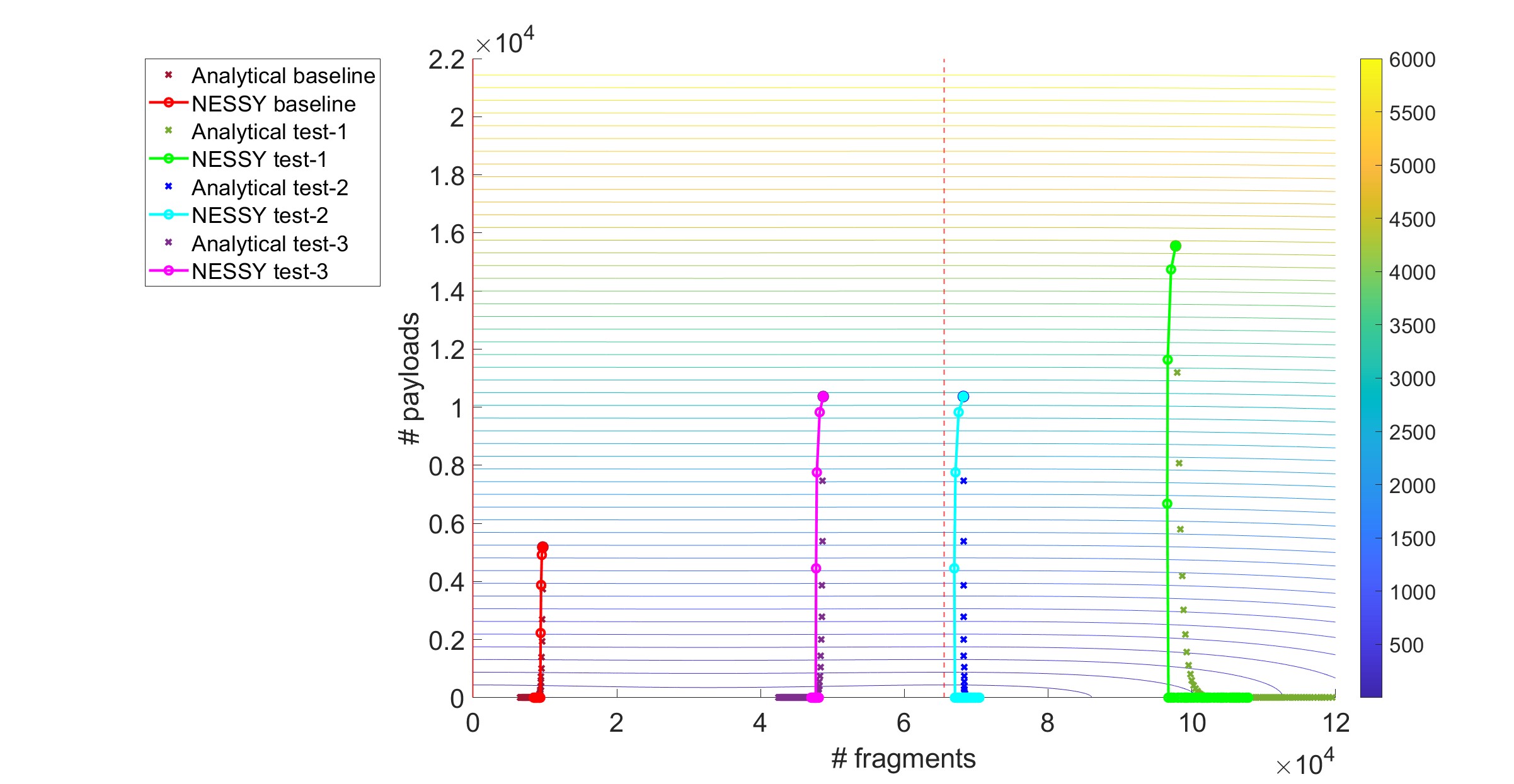
Figure 23: Carrying capacity analysis for the initial populations in Table 6 without new launches. Vertical red lines identify the equilibrium points.

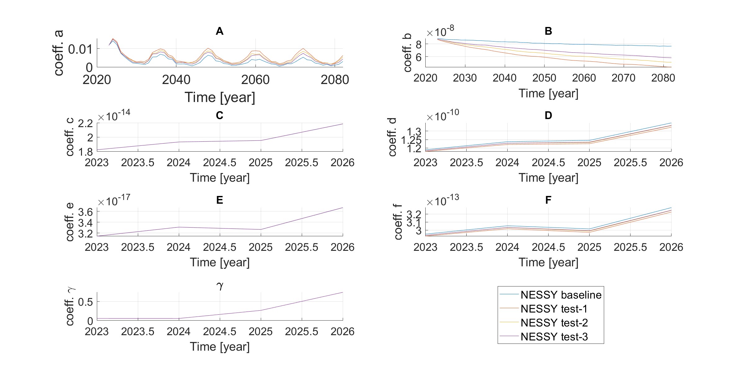
Figure 24: Coefficients evolution in time for the initial populations in Table 6, without new launches.

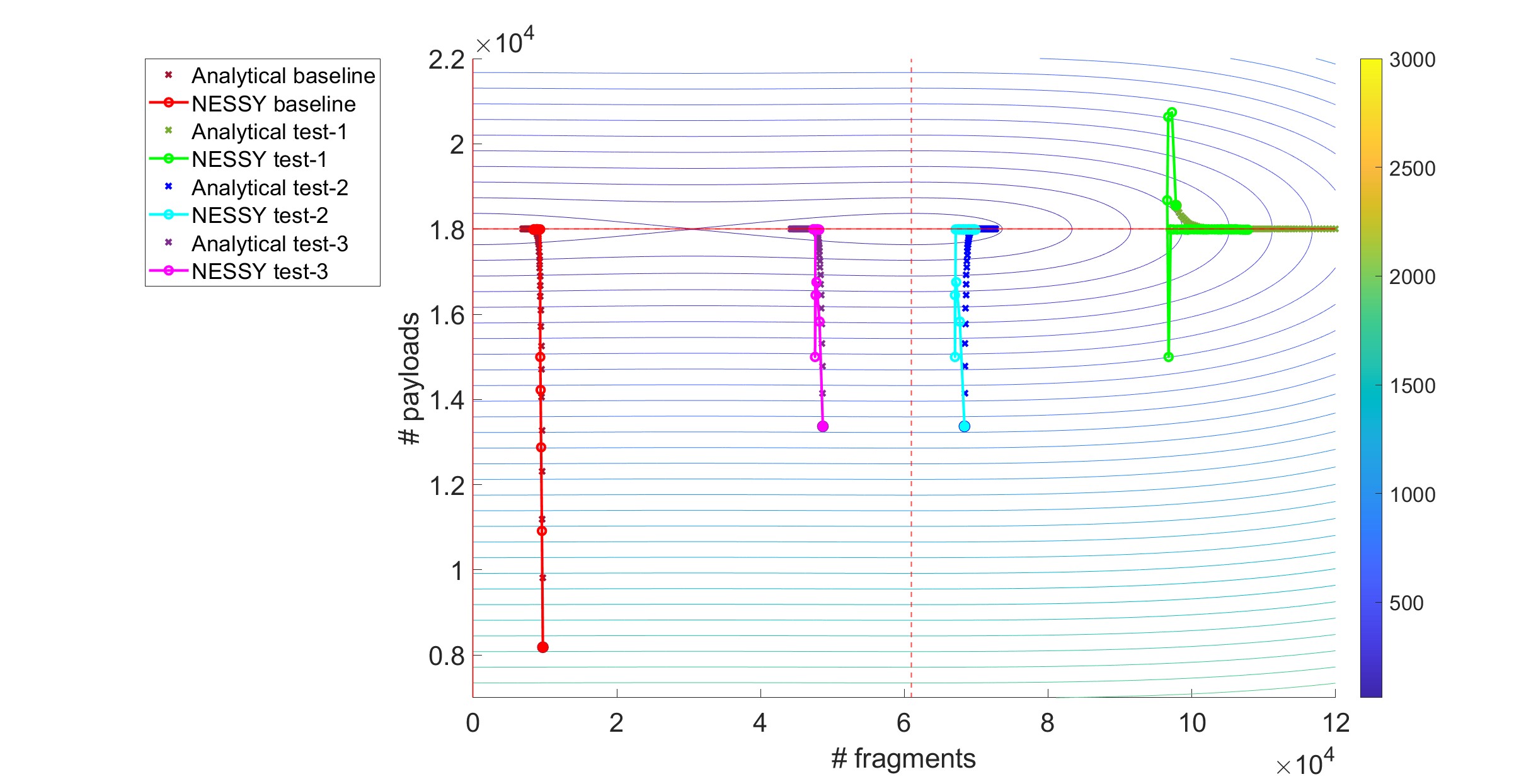
Figure 25: Carrying capacity analysis for the initial populations in Table 6, with new launches and $s_{CAM}$ = 99.99 %. Vertical red lines identify the equilibrium points.

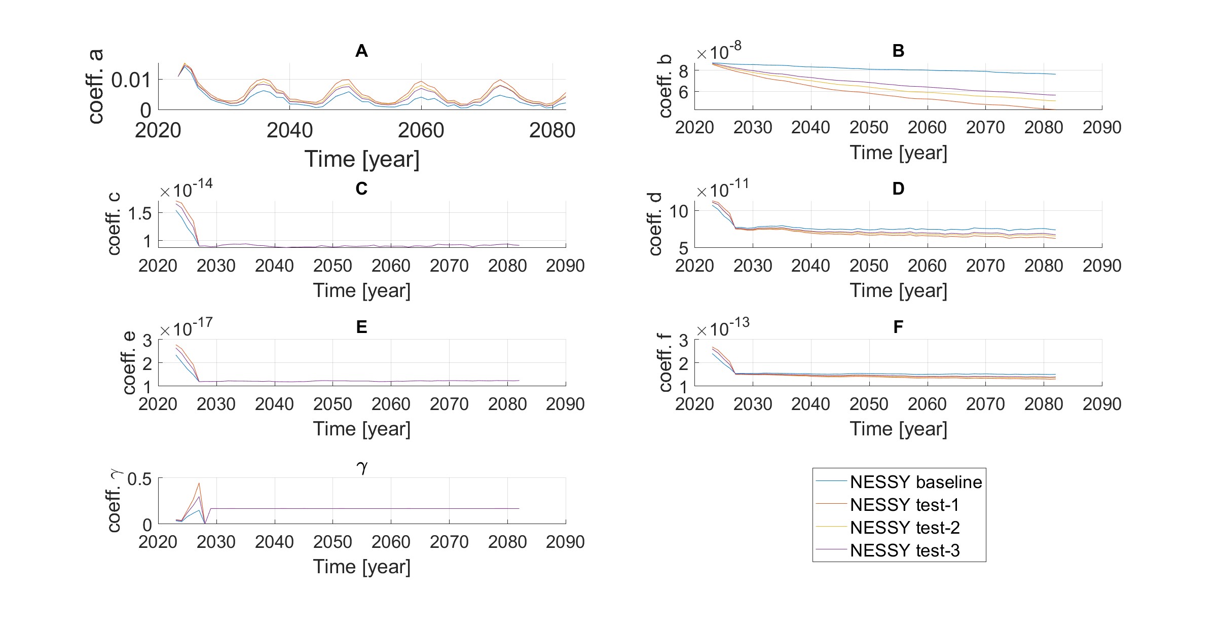
Figure 26: Coefficients evolution in time for the initial populations in Table 6 with new launches, for $s_{CAM}$ = 99.99 %.

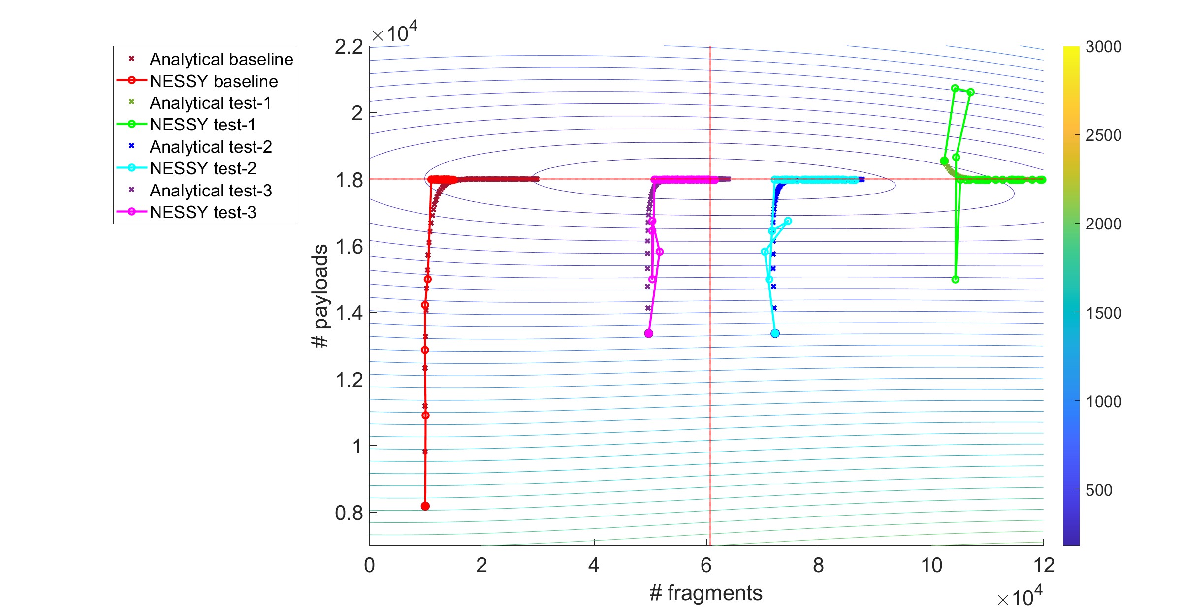
Figure 27: Carrying capacity analysis for the initial populations in Table 6, with new launches and $s_{CAM}$ = 0 %.

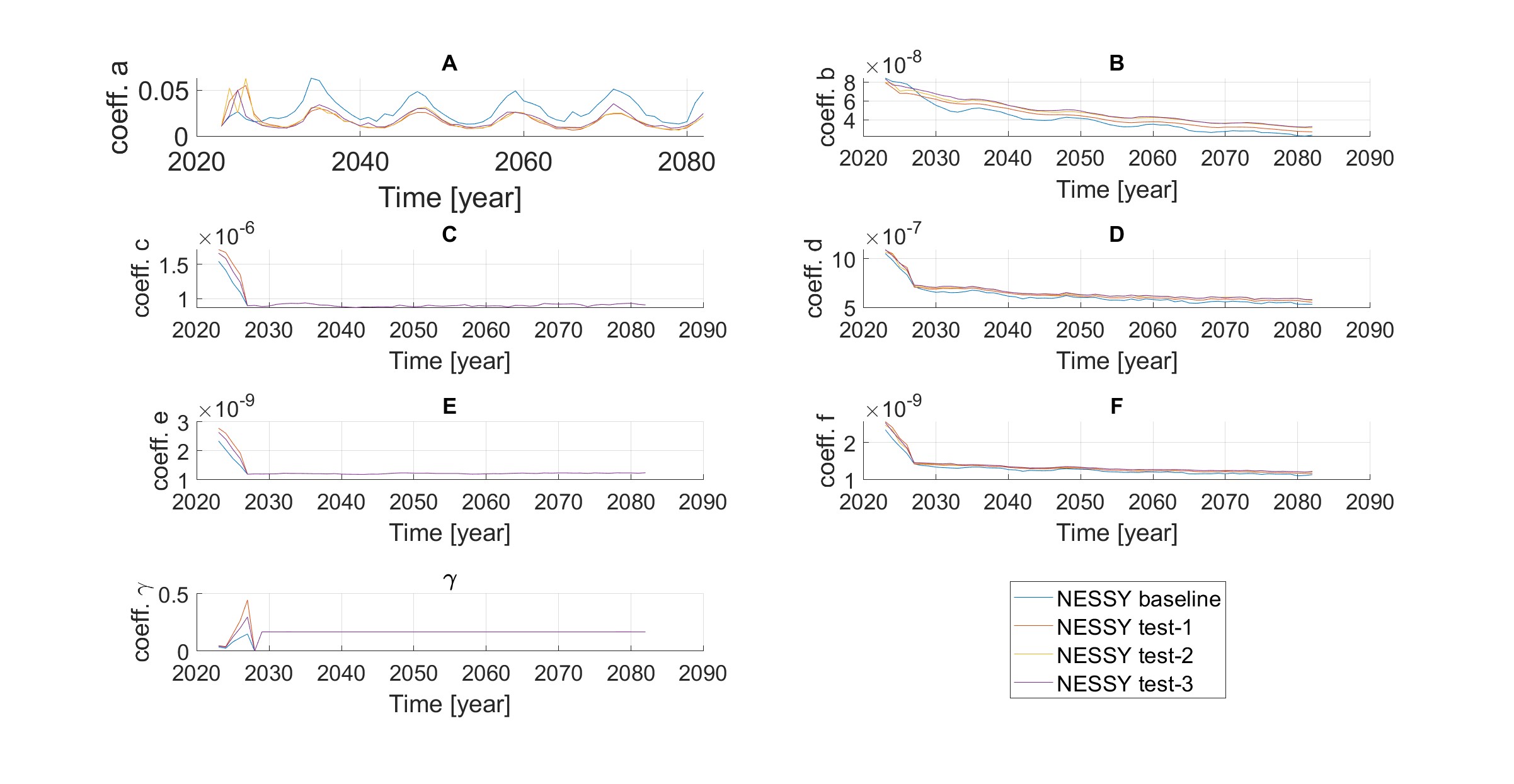
Figure 28: Coefficients evolution in time for the initial populations in Table 6 with new launches, for $s_{CAM}$ = 0 %.

Table 8: Equilibrium solutions and coefficients of system (35)

Case	Coefficients	Equilibria
Baseline	a = 0.00452577425958395 b = 6.90904299949640e-08 c = 1.97380609791357e-14 d = 1.24520883753270e-10 $\gamma$ = 0.279898522121588 $\lambda$ = 0 e = 3.34677170294235e-17 f = 3.05320507121121e-13	x=0; y=0 x=6.5505e+04; y=0
99.99% $s_{CAM}$	a = 0.00401396247805656 b = 6.57876829812750e-08 c = 9.04502294220185e-15 d = 7.04914968714949e-11 $\gamma$ = 0.166670665909938 $\lambda$ = 3000 e = 1.21252401882191e-17 f = 1.43180020023628e-13	x=0.0; y=1.8e4 x=6.0995e4; y=1.8e4
0% $s_{CAM}$	a= 0.0156698264653947 b = 4.03902373151070e-08 c = 9.04534200032272e-07 d = 6.10496583810926e-07 $\gamma$ = 0.166590355940308 $\lambda$ = 3000 e = 1.21254240683971e-09 f = 1.26183324512085e-09	y=1.8e4

7 Conclusions

This paper proposed a novel approach to investigate the global behaviour of the space environment and study the dynamic evolution of the relationships among space objects. Differently from previous works, we first developed a network model of the space environment and then derived the evolutionary equations from the structure of the network. The validation of the evolutionary equations showed that the proposed network model can provide results that are comparable to other state of the art long-term evolutionary models.

Furthermore, it was shown how the network model offers the unique ability to identify critical regions of the space environment. For instance, the node with the highest impact on the rest of the environment can be identified by analysing the in-degree and out-degree of each node. The nodes responsible for spreading or accumulating fragments can be identified through the out-degree or in-degree centrality measures. From the perspective of space operators, instead of focusing on the entire space environment, limited resources such as monitoring and mitigation efforts, can be strategically directed toward these identified priority space objects, optimising the allocation of resources based on their importance in comparison to others.

It was also shown how to derive the equilibrium solutions of the network dynamics and how these equilibrium solutions can be stable or unstable depending on the removal rate or the maneuverability of the resident objects. It was found that the space carrying capacity can be directly quantified as the ratio between the decay rate and the collision rate if only fragments are present in the environment. In this case an initial population above the capacity would diverge to infinity while an initial population below the capacity would converge to zero. If, on top of the fragments, new objects are launched into space, it was found that there are generally two equilibria, one stable and one unstable. One can then identify a region within which the environment would converge to a stable point. Outside this stability region, instead, the environment would diverge to infinity. In this paper, this analysis was limited to only two species and did not include lethal non trackable objects that would not lead to a catastrophic collision but would disable an active payload.

Future work will consider introducing other types of nodes, representing constellations, objects in high elliptical orbits, and other mitigation and remediation actions. Furthermore, explosions and small non-trackable lethal fragments need to be included in the evolutionary model together with other orbit regimes. New orbit regimes, like Geostationary Orbits or the cis-lunar environment, can be simply added as further sub-networks. This is the subject of current work.

References

- [1] Acciarini, G., Vasile, M.: A multi-layer temporal network model of the space environment. In: 71st International Astronautical Congress (2020)
- [2] Acciarini, G., Vasile, M.: A network-based evolutionary model of the space environment. In: 8th European Conference on Space Debris. pp. 1–9 (2021)
- [3] Adilov, N., Alexander, P.J., Cunningham, B.M.: An economic ”kessler syndrome”: A dynamic model of earth orbit debris. Economics Letters 166(MAY), 79–82 (2018)
- [4] Boley, A., Byers, M.: Satellite mega-constellations create risks in low earth orbit, the atmosphere and on earth. Nature Publishing Group (2021)
- [5] Bowman, B., Tobiska, W.K., Marcos, F., Huang, C., Lin, C., Burke, W.: A new empirical thermospheric density model jb2008 using new solar and geomagnetic indices. In: AIAA/AAS astrodynamics specialist conference and exhibit. p. 6438 (2008)
- [6] Bradley, A.M., Wein, L.M.: Space debris: Assessing risk and responsibility. Advances in Space Research 43(9), 1372–1390 (2009)
- [7] D’Ambrosio, A., Lifson, M., Linares, R.: The capacity of low earth orbit computed using source-sink modeling. arXiv preprint arXiv:2206.05345 (2022)
- [8] Dolado-Perez, J., Di Constanzo, R., Revelin, B.: Introducing medee–a new orbital debris evolutionary model. In: Proceeding of the 6th European Conference on Space Debris (2013)
- [9] D’Ambrosio, A., Linares, R.: Carrying capacity of low earth orbit computed using source-sink models. Journal of Spacecraft and Rockets 0(0), 1–17 (2024). https://doi.org/10.2514/1.A35729, https://doi.org/10.2514/1.A35729
- [10] D’Ambrosio, A., Servadio, S., Siew, P.M., Linares, R.: Novel source–sink model for space environment evolution with orbit capacity assessment. Journal of SpaceCraft and Rockets (2023)
- [11] Fleurence, R.L., Hollenbeak, C.S.: Rates and probabilities in economic modelling: transformation, translation and appropriate application. Pharmacoeconomics 25, 3–6 (2007)
- [12] Henning, G., Sorge, M., Peterson, G., Jenkin, A., McVey, J., Mains, D.: Impacts of large constellations and mission disposal guidelines on the future space debris environment. IAC-19, A6, 2, 7, x50024 (2019)
- [13] Jang, D., Gusmini, D., Siew, P.M., D’Ambrosio, A., Servadio, S., Machuca, P., Linares, R.: Monte carlo methods to model the evolution of the low earth orbit population. In: 33rd AAS/AIAA Space Flight Mechanics Meeting, Austin, TX. vol. 1 (2023)
- [14] Johnson, N.L., Krisko, P.H., Liou, J.C., Anz-Meador, P.D.: Nasa’s new breakup model of evolve 4.0. Advances in Space Research 28(9), 1377–1384 (2001)
- [15] Kessler, D.J., Cour-Palais, B.G.: Collision frequency of artificial satellites: The creation of a debris belt. Journal of Geophysical Research Space Physics 83(A6), 2637–2646 (1978)
- [16] Krag, H., Lemmens, S., Letizia, F.: Space traffic management through the control of the space environment’s capacity. In: Proceedings of the 1st IAA Conference on Space Situational Awareness (ICSSA) (2017)
- [17] Letizia, F., Colombo, C., Lewis, H., Krag, H.: Extending the ecob space debris index with fragmentation risk estimation (2017)
- [18] Letizia, F., Colombo, C., Lewis, H.G.: Collision probability due to space debris clouds through a continuum approach. Journal of Guidance, Control, and Dynamics 39(10), 2240–2249 (2016)
- [19] Letizia, F., Colombo, C., Lewis, H.G., Krag, H.: Assessment of breakup severity on operational satellites. Advances in Space Research 58(7), 1255–1274 (2016). https://doi.org/https://doi.org/10.1016/j.asr.2016.05.036, https://www.sciencedirect.com/science/article/pii/S0273117716302393
- [20] Lewis, H.G., Newland, R.J., Swinerd, G.G., Saunders, A.: A new analysis of debris mitigation and removal using networks. Acta Astronautica 66(1-2), 257–268 (2010)
- [21] Liou, J.C., Hall, D., Krisko, P., Opiela, J.: Legend–a three-dimensional leo-to-geo debris evolutionary model. Advances in Space Research 34(5), 981–986 (2004)
- [22] Liou, J.C., Johnson, N.L.: Risks in space from orbiting debris (2006)
- [23] Liou, J.C., Johnson, N.L.: A sensitivity study of the effectiveness of active debris removal in leo. Acta Astronautica 64(2-3), 236–243 (2009)
- [24] Liou, J.C., Kessler, D.J., Matney, M., Stansbery, G.: A new approach to evaluate collision probabilities among asteroids, comets, and kuiper belt objects. In: Lunar and Planetary Science Conference. p. 1828 (2003)
- [25] Lucken, R., Giolito, D.: Collision risk prediction for constellation design. Acta Astronautica 161, 492–501 (2019)
- [26] Martinusi, V., Dell’Elce, L., Kerschen, G.: Analytic propagation of near-circular satellite orbits in the atmosphere of an oblate planet. Celestial Mechanics and Dynamical Astronomy 123, 85–103 (2015)
- [27] McKnight, D., Lorenzen, G.: Collision matrix for low earth orbit satellites. Journal of Spacecraft and Rockets 26(2), 90–94 (1989)
- [28] Muelhaupt, T.J., Sorge, M.E., Morin, J., Wilson, R.S.: Space traffic management in the new space era. Journal of Space Safety Engineering 6(2), 80–87 (2019)
- [29] Murakami, D.D., Nag, S., Lifson, M., Kopardekar, P.H.: Space traffic management with a nasa uas traffic management (utm) inspired architecture. In: AIAA Scitech 2019 Forum. p. 2004 (2019)
- [30] Office, E.S.D.: DISCOSweb (2024), https://discosweb.esoc.esa.int/
- [31] Oltrogge, D.L., Alfano, S.: The technical challenges of better space situational awareness and space traffic management. Journal of Space Safety Engineering 6(2), 72–79 (2019). https://doi.org/https://doi.org/10.1016/j.jsse.2019.05.004, https://www.sciencedirect.com/science/article/pii/S2468896719300333, space Traffic Management and Space Situational Awareness
- [32] Pardini, C., Anselmo, L.: Review of past on-orbit collisions among cataloged objects and examination of the catastrophic fragmentation concept. Acta Astronautica 100, 30–39 (2014)
- [33] Rodriguez-Fernandez, V., Sarangerel, S., Siew, P.M., Machuca, P., Jang, D., Linares, R.: Towards a machine learning-based approach to predict space object density distributions. In: AIAA SCITECH 2024 Forum. p. 1673 (2024)
- [34] Romano, M., Carletti, T., Daquin, J.: The resident space objects network: A complex system approach for shaping space sustainability. The Journal of the Astronautical Sciences 71(4) (Jun 2024). https://doi.org/10.1007/s40295-024-00449-4, http://dx.doi.org/10.1007/s40295-024-00449-4
- [35] Rossi, A., Anselmo, L., Pardini, C., Valsecchi, G., Jehn, R.: Analysis of the Space Debris Environment with SDM 3.0. https://doi.org/10.2514/6.IAC-04-IAA.5.12.1.06, https://arc.aiaa.org/doi/abs/10.2514/6.IAC-04-IAA.5.12.1.06
- [36] Rossi, A., Valsecchi, G., Alessi, E.: The criticality of spacecraft index. Advances in Space Research 56(3), 449–460 (2015)
- [37] Stein, L.: LEO SATCOM report (Mar 2022), https://www.primemoverslab.com/resources/ideas/leo-satcom.pdf
- [38] Sturza, M., Carretero, G.S.: Design trades for environmentally friendly broadband leo satellite systems (2021)
- [39] Talent, D.L.: Analytic model for orbital debris environmental management. Journal of Spacecraft and Rockets 29(4), 508–513 (1992). https://doi.org/10.2514/3.25493, https://doi.org/10.2514/3.25493
- [40] Virgili, B.B.: Delta debris environment long-term analysis. In: Proceedings of the 6th International Conference on Astrodynamics Tools and Techniques (ICATT) (2016)
- [41] Walker, R., Stokes, P., Wilkinson, J., Swinerd, G.: Enhancement and validation of the ides orbital debris environment model. Space Debris 1, 1–19 (1999)
- [42] Wang, X.w., Liu, J.: An introduction to a new space debris evolution model: Solem. Advances in Astronomy 2019, 1–11 (2019)
- [43] Wang, Y., Wilson, C., Vasile, M.: Multi-layer temporal network model of the space environment. In: 2023 AAS/AIAA Astrodynamics Specialist Conference (2023)
- [44] Wilson, C.J., Vasile, M., Feng, J., McNally, K., Antón, A., Letizia, F.: Modelling future launch traffic and its effect on the leo operational environment. In: AIAA SCITECH 2024 Forum. p. 1814 (2024)
- [45] Zhang, J., Yuan, Y., Yang, K., Li, L.: Long-term evolution of the space environment considering constellation launches and debris disposal. IEEE Transactions on Aerospace and Electronic Systems pp. 1–17 (2023). https://doi.org/10.1109/TAES.2023.3274097