Navigating Extremes:
Dynamic Sparsity in Large Output Spaces

Abstract

In recent years, Dynamic Sparse Training (DST) has emerged as an alternative to post-training pruning for generating efficient models. In principle, DST allows for a more memory efficient training process, as it maintains sparsity throughout the entire training run. However, current DST implementations fail to capitalize on this in practice. Because sparse matrix multiplication is much less efficient than dense matrix multiplication on GPUs, most implementations simulate sparsity by masking weights. In this paper, we leverage recent advances in semi-structured sparse training to apply DST in the domain of classification with large output spaces, where memory-efficiency is paramount. With a label space of possibly millions of candidates, the classification layer alone will consume several gigabytes of memory. Switching from a dense to a fixed fan-in sparse layer updated with sparse evolutionary training (SET); however, severely hampers training convergence, especially at the largest label spaces. We find that poor gradient flow from the sparse classifier to the dense text encoder make it difficult to learn good input representations. By employing an intermediate layer or adding an auxiliary training objective, we recover most of the generalisation performance of the dense model. Overall, we demonstrate the applicability and practical benefits of DST in a challenging domain — characterized by a highly skewed label distribution that differs substantially from typical DST benchmark datasets — which enables end-to-end training with millions of labels on commodity hardware.

1 Introduction

Recent research Frankle and Carbin (2018); Frankle et al. (2020); Malach et al. (2020); Chen et al. (2021a) has demonstrated that densely-connected neural networks contain sparse subnetworks — often dubbed “winning lottery tickets” — that can deliver performance comparable to the full networks but with substantially reduced compute and memory demands. Unlike conventional techniques that start with a trained dense model and employ iterative pruning or one-shot pruning, Dynamic Sparse Training (DST) Mocanu et al. (2018); Evci et al. (2020); Liu et al. (2021a) initializes the a sparse architecture and dynamically explores subnetwork configurations through periodic pruning and regrowth, typically informed with heuristic saliency criteria such as weight and gradient magnitudes. This approach is particularly advantageous in scenarios constrained by a fixed memory budget during the training phase, making DST viable across various domains Chen et al. (2021a); Dietrich et al. (2021); Liu et al. (2021b). For instance, in reinforcement learning Tan et al. (2022); Graesser et al. (2022), DST has been shown to significantly outperform traditional dense models. Additionally, models trained using DST often exhibit enhanced robustness Guo et al. (2018); Özdenizci and Legenstein (2021); Chen et al. (2021b); Diffenderfer et al. (2021); Liu et al. (2022). However, the application of DST comes with challenges, notably prolonged training times; for example, RigL Evci et al. (2020) and ITOP Liu et al. (2021a) require up to five and two times as many optimization steps during training, respectively, to match the generalisation performance of dense networks at high sparsity levels ($\geq 80\%$). The prolonged training time in these works is often linked to the need for in-time overparameterization Liu et al. (2021a) and poor gradient flow in sparse networks. Recent advances Evci et al. (2022); Price and Tanner (2021); Curci et al. (2021) aimed at improving gradient flow have been introduced to mitigate these extended training durations, enhancing the practicality of DST methodologies.

In this paper, we investigate the integration of DST into extreme multi-label classification (XMC) Bhatia et al. (2016); Babbar and Schölkopf (2017); Prabhu et al. (2018). XMC problems are characterized by a very large label space, with hundreds of thousands to millions of labels, often in the same order of magnitude as the number of training examples. The large label space in such problems makes calculating logits for every label a very costly operation. Consequently, contemporary XMC methodologies Jiang et al. (2021); You et al. (2019); Kharbanda et al. (2022); Dahiya et al. (2021, 2023); Zhang et al. (2021); Schultheis and Babbar (2022); Qaraei and Babbar (2024) utilize modular and sampling-based techniques to achieve sublinear compute costs. However, these strategies do not help in addressing the immense memory requirement associated with the classification layer, which can be enormous: for an embedding dimension of 768, one million labels lead to a memory consumption of about 12 GB taking into account weights, gradients, and optimizer state. Memory efficiency in XMC has been pursued in the context of sparse linear models (Babbar and Schölkopf, 2017, 2019; Yen et al., 2016) or by using label-hashing (Medini et al., 2019), but such methods do not yield predictive performance competitive with modern transformer-based deep networks. Schultheis and Babbar (2023) demonstrated that applying a DST method to the extreme classification layer can lead to substantial memory savings at marginal accuracy drops; however, that work presupposed the existence of fixed, well-trained document embeddings which output the hidden representations used by the classifier, whereas in a realistic setting these need to be trained jointly.

Recently, Jain et al. (2023) demonstrated that full end-to-end training of XMC models can be very successful, given sufficient computational resources. To make this accessible to consumer-grade hardware, we propose to switch the dense classification layer to a DST-trained sparse layer. Not only does this result in a training procedure that allows XMC models to be trained in a GPU-memory constrained setting, but it also provides an evaluation of DST algorithms outside typical, well-behaved benchmarks. This is particularly important since recent works (Liu et al., 2023; Jaiswal et al., 2024) have found that sparse training algorithms that appear promising on standard benchmark datasets may fail to produce adequate results on actual real-world tasks. As such, we introduce XMC problems — with their long-tailed label distribution (Jain et al., 2016; Buvanesh et al., 2023; Schultheis et al., 2024), missing labels (Jain et al., 2016; Qaraei et al., 2021; Schultheis et al., 2022; Schultheis and Babbar, 2021), and general training data scarcity issues (Babbar and Schölkopf, 2019) — as a new setting to challenge current sparsity approaches.

Figure 1: Model configurations and performance comparisons at various sparsity levels. The left panel illustrates our model configurations: ‘S’ represents a semi-structured fixed fan-in sparse layer, ‘W’ denotes an intermediate layer, and ‘Aux’ refers to an auxiliary head of meta-classifiers. These configurations help maintain performance as the label space size increases from 31K to 670K and beyond. The right panel demonstrates the comparative precision at 1 for our model against other methods across increasing levels of sparsity on the Amazon670K dataset.

In fact, direct application of existing DST methods yields unsatisfactory results on XMC tasks due to typically noisy data and poor gradient signal propagation through the sparse classifier, slowing training convergence to an extent that it is not practically useful. Consequently, we follow Schultheis and Babbar (2023) and adapt the model architecture by integrating an intermediate layer that is larger than the embedding from the encoder but still significantly smaller than the final output layer. While this was found to be sufficient to achieve good results with fixed encodings, it fails if the encoder is a trainable transformer (Devlin et al., 2018; Sanh, 2019) for label spaces with more than one hundred thousand elements, particularly at high levels of sparsity. The primary challenge arises from the noisy gradients prevalent at the onset of training, which are inadequate for guiding the fine-tuning of the encoder effectively. To mitigate this issue, we introduce an auxiliary loss. This loss uses a more coarse-grained objective, assigning instances to clusters of labels, where scores for each cluster are calculated using a dense classification layer. This auxiliary component stabilizes the gradient flow and enhances the encoder’s adaptability during the critical early phases of training and is turned off during later epochs to not interfere with the main task. Figure 1 illustrates the architectural changes that ensure good training performance at different label space sizes and sparsity levels.

To materialize actual memory savings, we propose Spartex, which uses semi-structured sparsity (Lasby et al., 2024; Schultheis and Babbar, 2023) with a fixed fan-in constraint, together with magnitude-based pruning and random regrowth (SET (Mocanu et al., 2018)), which does not require any additional memory buffers. In our experiments, we show that Spartex achieves a 3.4-fold reduction of GPU memory requirements from 46.3 to $13.5\text{\,}\mathrm{GiB}$ for training on the Amazon-3M (Bhatia et al., 2016) dataset, with only an approximately 3% reduction in predictive performance. In comparison, a naïve parameter reduction using a bottleneck layer (i.e., a low-rank classifier) at the same memory budget decreases precision by about 6%.

Our primary contributions are as follows:

• Enhancements in training efficiency: We propose novel modifications to the conventional DST framework that significantly curtail training durations while concurrently delivering competitive performance metrics when benchmarked against dense model baselines and other specialized XMC methodologies. These enhancements are pivotal in demonstrating DST’s scalability and efficiency to large label spaces.

• Optimized hardware utilization: We provide PyTorch bindings for custom CUDA kernels which enable a streamlined integration of memory-efficient sparse training into an existing XMC pipeline. This implementation enables the deployment of our training methodologies on conventional, commercially available hardware, thus democratizing access to state-of-the-art XMC model training.

• Robustness to Label distribution challenges: Our empirical results demonstrate that the DST framework, as adapted and optimized by our modifications, can effectively manage datasets characterized by label imbalances and the presence of missing labels, with minimal performance degradation for tail labels.

2 Dynamic Sparse Training for Extreme Multi-label Classification

2.1 Background

Problem setup

Given a multi-label training dataset with $N$ samples, $\mathcal{D}=\{(x_{i},P_{i})_{i=1}^{N}\}$, where $L$ represents the total number of labels, and $P_{i}\subset[L]$ denotes a subset of relevant labels associated with the data point $x_{i}\in\chi$. Typically, the instances are text based, such as the contents of a Wikipedia article (Bhatia et al., 2016) or the title of a product on Amazon (McAuley and Leskovec, 2013) with labels corresponding to Wikipedia categories and frequently bought together products, respectively, for example. Traditional XMC methods used to handle labels the same way as is typically done in other fields, as featureless integers.

However, the labels themselves usually carry some information, e.g., a textual representation, as the following examples, taken from (i) LF-AmazonTitles-131K (recommend related products given a product name) and (ii) LF-WikiTitles-500K (predict relevant categories, given the title of a Wikipedia page) illustrate:

Example 1: For “Nintendo Land” on Amazon, we have available: Mario Tennis Ultra Smash(Nintendo Wii U) $|$ Star Fox Zero (Nintendo Wii U), as the recommended products.

Example 2: For the “2024 United States presidential election” Wikipedia page, we have the available categories: Joe Biden $|$ Joe Biden 2024 presidential campaign $|$ Donald Trump $|$ Donald Trump 2024 presidential campaign $|$ Kamala Harris $|$ November 2024 events in the United States.

Consequently, more recent XMC approaches have started to take these label features into account to alleviate the data scarcity problems (Dahiya et al., 2021; Mittal et al., 2021).

XMC and DST

The XMC models are typically comprised of two main components: (i) an encoder $\mathcal{E}_{\theta}:\chi\rightarrow\mathbb{R}^{d}$, which embeds data points into a $d$-dimensional real space, primarily utilizing a transformer architecture (Vaswani et al., 2017) and (ii) A One-vs-All classifier $W=\{w_{l}\}_{l\in[L]}$, where $w_{l}$ denotes the classifier for label $l$, integrated as the last layer of the neural network in end-to-end training settings. In a typical DST scenario, one would sparsify the language model used as the encoder, potentially even leaving the classifier fully dense (Kurtic et al., 2024). However, in XMC, most of the networks weights are in the classifier layer, so in order to achieve a reduction in memory consumption, its weight matrix $W_{s}=\{w_{l}^{s}\}_{l\in[L]}$ must be sparsified.

This sparse layer $W_{s}$ is then periodically updated in a prune-regrow-train loop, that is, every $\Delta T$ steps, a fraction of active weights are pruned and the same number of inactive weights are regrown. The updated sparse topology is then trained with regular gradient descent for the next $\Delta T$ steps. There are many possible choices for pruning and regrowth criteria (Hoefler et al., 2021); to keep memory consumption low, however, we need to choose a method that does not require auxiliary buffers proportional to the size of the dense layer. This excludes methods such as requiring second-order information (Hassibi and Stork, 1992), or tracking of dense gradients or other per-weight information (Dai et al., 2019; Dettmers and Zettlemoyer, 2019; Lin et al., 2020). Evci et al. (2020) argue that RigL only needs dense gradients in an ephemeral capacity — they can be discarded as soon as the regrowth step for the current layer is done, but before the regrow step of the next layer is started — but in the XMC setup, the prohibitively large memory consumption arises already from a single layer. Therefore, we select magnitude-based pruning and random regrowth (Mocanu et al., 2018). Magnitude-based pruning has been shown to be a remarkably strong baseline (Nowak et al., 2024).

However, to actually achieve efficient training with these algorithms in the XMC setting, several challenges need to be overcome as discussed below.

2.2 Memory-Efficient Training: Fixed Fan-In Sparse Layer

Unstructured sparsity is notoriously difficult to speed-up on GPUs Gale et al. (2020), and consequently most DST studies simulate sparsity by means of a binary mask (Curci et al., 2021; Lee et al., 2023). On the other hand, highly structured sparsity, such as 2:4 sparsity (Castro et al., 2023), enjoys hardware acceleration and memory reduction (Mishra et al., 2021), but results in deteriorated model accuracy compared to unstructured sparsity (Liu and Wang, 2023). As a compromise, semi-structured sparsity (Lasby et al., 2024; Schultheis and Babbar, 2023) imposes a fixed fan-in to each neuron. This eliminates work imbalances between different neurons, leading to an efficient and simple storage format for sparse weights, where each sparse weight needs only a single integer index. For 32-bit floating point weights with 16-bit indices (i.e., at most 65k features in the embedding layer), this leads to a 50% storage overhead for sparse weights; however, for training, gradient and two momentum terms are needed, which share the same indexing structure, reducing the effective overhead to just 12.5%.

While fixed fan-in provides substantial speed-ups for the forward pass, due to the transposed matrix multiplication required for gradients, it does not give any direct benefits for the backwards pass. Fortunately, when used for the classification matrix, the backpropagated gradient is the loss derivative, which will exhibit high activation sparsity if the loss function is hinge-like (Schultheis and Babbar, 2023). In the enormous label space of XMC, for each instance only a small subset of labels will be hard negatives. The rest will be easily classified as true negatives, and not contribute to the backward pass.

As additional measures to keep the memory consumption low, we enable torch.amp automatic mixed-precision training (Micikevicius et al., 2018) and activation checkpointing (Chen et al., 2016) for the BERT encoder.

2.3 Improved Gradient Flow: Auxiliary Objective

We find that, despite using a fully dense network, training the encoder using gradients backpropagated from a sparse classification layer requires more optimization steps to converge compared with to a dense classification layer. This compounds with the already-increased number of epochs required for DST (Evci et al., 2020; Liu et al., 2021a), further increasing the training duration of end-to-end XMC training, which requires longer training than comparable modularized or shortlisting-based methods (Jain et al., 2023). Furthermore, the intermediate activations in the transformer-based encoder also take up a considerable amount of GPU memory, so to meet memory budgets, we may need to switch to smaller batch sizes or employ activation checkpointing, increasing the per-step time.

Therefore, we need to improve gradient flow through the sparse layer. Schultheis and Babbar (2023) inserted a large intermediate layer preceding the actual classifier to achieve significant improvements in performance. While this method is sufficient to achieve good results with fixed encodings, we observe that it fails to perform well if the encoder is a trainable transformer (Devlin et al., 2018; Sanh, 2019) for label spaces with more than one hundred thousand elements, particularly for high sparsity levels. Therefore, we instead propose to use the label shortlisting task that is typical for XMC pipelines as an auxiliary objective to generate informative gradients for the encoder.

Rethinking the role of clusters and meta-classifier in XMC

Many prevailing XMC methods, apart from learning the per-label classifiers $W=\{w_{l}\}_{l\in[L]}$ for the extreme task, also employ a meta-classifier. The meta-classifier learns to classify over clusters of similar labels that are created by recursively partitioning the label set into equal parts using, for example, balanced $k$-means clustering Jiang et al. (2021); Kharbanda et al. (2022); Zhang et al. (2021); You et al. (2019); Kharbanda et al. (2023). These meta-classifiers are primarily used for label shortlisting or retrieval prior to the final classification or re-ranking at the extreme scale. We investigated the impact on the final performance of the extreme task when the labels are randomly assigned to the clusters (instead of the following the k-means objective). We observed that such reassignments do not negatively affect the extreme task’s performance (detailed of this observation are shown in Appendix E). This leads us to hypothesize that beyond merely shortlisting labels, meta-classifier branch of the XMC training pipelines provides useful gradient signals during encoder training, which is particularly crucial for larger datasets with $\mathcal{O}(10^{6})$ labels such as Amazon-670K (Figure 1) and Amazon-3M.

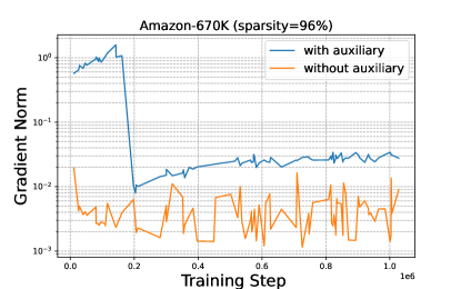
Figure 2: Gradient Flow of the encoder during training with and without Auxiliary Objective.

Auxiliary objective and DST convergence for XMC

Towards addressing the challenge of gradient instability, we augment our training pipeline with an additional meta-classifier branch which aids gradient information during back-propagation. This is especially useful during the initial training phase where the fixed-fan-in sparse layer tends to encounter difficulties. Importantly, in our model the output layer operates independently of the meta-classifier’s outputs, enabling a seamless end-to-end training process.

Although a meta-classifier assists during the initial stages of training, maintaining it throughout the entire training process can deteriorate the encoder’s representation quality. This degradation occurs because the task associated with the meta classifiers differs from the final task, yet both share the same encoder. Similar observations have been noted in related studies Kharbanda et al. (2022). To address this issue, we implement a decaying scaling factor on the auxiliary loss, gradually reducing its influence as training progresses.

The impact of the auxiliary branch on the norm of the gradient in the encoder is demonstrated in Figure 2 for the Amazon-670K dataset. The larger gradient signal speeds up initial learning, but it is misaligned with the true objective, so is gradually turned off at around 200k steps. Furthermore, the improvement in prediction performance, as reflected in Figure 1 (right panel), reinforces the quality of gradient as compared to the training pipeline without the auxiliary objective.

3 Experiments and discussion

3.1 Datasets

In this study, we evaluate our proposed modifications of DST under the extreme classification setting across a diverse set of large-scale datasets, including Wiki10-31K (Zubiaga, 2012), Wiki-500K (Bhatia et al., 2016), Amazon-670K (McAuley and Leskovec, 2013), and Amazon-3M (McAuley et al., 2015). The datasets are publicly available at the Extreme Classification Repository. These were selected due to their inherent complexity and the challenges posed by their long-tailed label distributions, which are emblematic of real-world data scenarios and test the robustness of DST methodologies. Further validation of our approach is conducted using the datasets LF-AmazonTitles-131K and LF-WikiSeeAlso-320K. These datasets are particularly relevant due to their augmentation with rich label metadata and their concise text formats, traits that have gained considerable traction in the XMC research community of late. The datasets’ detailed statistical profiles are delineated in Table 1.

Table 1: Statistics of XMC Datasets with and without Label Features. This table presents a comparison across various datasets, detailing the total number of training instances ($N$), unique labels ($L$), number of test instances ($N^{\prime}$), average label count per instance ($\overline{L}$), and average data points per label ($\hat{L}$).

Dataset	$N$	$L$	$N^{\prime}$	$\overline{L}$	$\hat{L}$
Datasets without Label Features
Wiki10-31K	$14,146$	$30,938$	$6616$	$18.64$	$48.52$
Wiki-500K	$1,779,881$	$501,070$	$769,421$	$4.75$	$16.86$
Amazon-670K	$490,449$	$670,091$	$153,025$	$5.45$	$3.99$
Amazon-3M	$1,717,899$	$2,812,281$	$742,507$	$36.17$	$31.64$
Datasets with Label Features
LF-AmazonTitles-131K	$294,805$	$131,073$	$134,835$	$5.15$	$2.29$
LF-WikiSeeAlso-320K	$693,082$	$312,330$	$177,515$	$4.67$	$2.11$

3.2 Baselines and evaluation metrics

To ensure a comprehensive and fair evaluation of our proposed DST methodologies applied to XMC problems, we compare our proposed framework, Spartex, across three principal categories of baseline methods:

1. Dense Models : Consistent with traditional DST evaluations, we compare the performance of our sparse models against their dense counterparts.

2. Dense Models with bottleneck layer : This category (referred to as Dense BN in Table 2) includes dense models with the same number of parameters as our proposed DST method by having a bottleneck layer with the same dimensionality as the FFI size. This ensures that comparisons focus on the impact of sparsity rather than differences in model size or capacity.

3. XMC Methods: For datasets devoid of label features, we benchmark against the latest transformer-based models such as CascadeXML Kharbanda et al. (2022), LightXML Jiang et al. (2021), and XR-Transformer. For datasets that incorporate label features, our comparison includes leading Siamese methods like SiameseXML Dahiya et al. (2021) and NGAMEDahiya et al. (2023), as well as other relevant transformer-based approaches.

Notably, Renee Jain et al. (2023) qualifies as both a dense model and a state-of-the-art XMC method. However, in some instances, Renee employs larger encoders (e.g., Roberta-Large Liu (2019)). To maintain consistency and fairness in our evaluations, we exclude configurations employing larger encoders from this analysis. For conceptual validation, we used RigLEvci et al. (2020) on datasets with label spaces up to 670K.

As is standard in XMC literature, we compare the methods on metrics which only consider prediction at top-k slots. This includes : Precision@k and its propensity-scored variant (which is more sensitive to performance on tail-labels). The details of these metrics are given in Appendix A.

3.3 Empirical performance

Table 2 presents our primary results on the datasets, compared with the aforementioned baselines. The performance metrics for XMC baselines are reported from their original papers. However, for peak memory consumption, we re-ran these baselines in half precision with the same batch size, as all baselines are also evaluated in half precision. Following DST protocols, we extended the training duration for RigL, Dense Bottleneck, and our method to twice the number of steps used for dense models. Certain baselines (referred to as OOM) could not scale to the Amazon-3M dataset. Our results demonstrate that our method significantly reduces memory usage while maintaining competitive performance. On the Amazon-3M dataset, our approach delivers comparable performance to dense models while achieving a 3.4-fold reduction in memory usage and a 5.-fold reduction compared to the XMC baseline. Furthermore, within the memory-efficient model regime, our method consistently outperforms the Dense Bottleneck model. To further validate the robustness of our approach, we evaluated it on the label features datasets, as shown in Table 3. Notably, as the label space size increases, we need to adjust to a comparatively lower sparsity to maintain performance, discussed in detail in subsequent sections.

Table 2: Comparison with different methods. Comparing our sparse model against its dense counterpart and with state-of-the-art XMC methods on Wiki10-31K, Wiki-500K, Amazon-670K and Amazon-3M datasets. $M_{\mathrm{tr}}(\mathrm{GiB})$ indicates peak GPU memory consumption during training.

Method	Sparsity (%)	P@1	P@3	P@5	$M_{\mathrm{tr}}$ $(\mathrm{GiB})$	Sparsity (%)	P@1	P@3	P@5	$M_{\mathrm{tr}}$ $(GiB)$
		Wiki10-31K					Wiki-500K
AttentionXML	-	87.1	77.8	68.8	8.2	-	75.1	56.5	44.4	13.1
LightXML	-	87.8	77.3	68.0	16.5	-	76.2	57.2	44.1	14.6
CascadeXML	-	88.4	78.3	68.9	8.2	-	77.0	58.3	45.1	18.8
Dense	-	87.8	77.2	68.1	2.5	-	78.5	59.2	45.6	9
Dense BN	-	86.7	76.3	66.0	2.1	-	73.8	55.1	42.0	4.3
RigL	92	87.7	77.3	67.7	2.6	83	74.5	54.7	41.8	9.7
Spartex	92	88.6	77.7	67.4	2.1	83	76.7	57.8	44.5	4.1
		Amazon-670K					Amazon-3M
AttentionXML	-	45.7	40.7	36.9	10.7	-	49.1	46.0	43.9	71.2
LightXML	-	47.1	42.0	38.2	11.2	-	-	-		OOM
CascadeXML	-	48.5	43.7	40.0	18.3	-	51.3	49.0	46.9	87.0
Dense	-	49.8	44.2	40.1	11.5	-	53.4	50.6	48.5	46.3
Dense BN	-	44.5	39.7	36.1	4.0	-	47.0	44.6	42.7	13.1
RigL	83	45.2	38.7	36.0	12.4	83	-	-	-	OOM
Spartex	83	47.1	41.8	38.0	3.7	83	50.2	47.1	44.8	13.5

Table 3: Comparison on label feature datasets LF-AmazonTitles-131K and LF-WikiSeeAlso-320K. $M_{\mathrm{tr}}(\mathrm{GiB})$ indicates peak GPU memory usage during training.

Method	Sparsity (%)	P@1	P@3	P@5	$M_{\mathrm{tr}}$ $(\mathrm{GiB})$	Sparsity (%)	P@1	P@3	P@5	$M_{\mathrm{tr}}$ $(GiB)$
		LF-AmazonTitles-131K					LF-WikiSeeAlso-320K
LightXML	-	35.6	24.2	17.5	11.6	-	34.5	22.3	16.8	13.5
ECLARE	-	40.7	27.5	19.9	8.8	-	40.6	26.9	20.1	10.2
SiameseXML	-	41.4	27.9	21.2	7.1	-	42.2	28.1	21.4	8.9
NGAME	-	46	30.3	21.5	9.0	-	47.7	31.6	23.6	19.3
DEXML	-	42.5	-	20.6	30.2	-	46.1	29.9	22.3	56.1
Renee (Dense)	-	46.1	30.8	22	3.0	-	47.9	31.9	24.1	9.1
Dense BN	-	39.2	25.7	18.2	2.2	-	44.5	28.4	21.5	6.0
RigL	83	43.0	28.6	20.4	3.2	67	44.9	29.0	21.7	9.2
Spartex	83	44.5	29.8	21.3	2.2	67	46.0	29.9	22.1	6.1

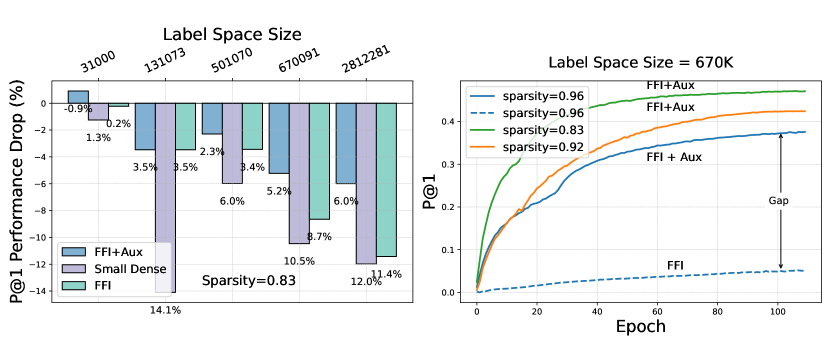
Figure 3: left: Comparison of performance declines as the size of the label space increases, given a fixed sparsity. right: Performance of our model at different epochs, across various sparsity ratios.

3.4 Adapting to increased sparsity and label size: the role of auxiliary objective

The DST approach is widely recognized to be problematic when dealing with high sparsity levels ($\geq 90\%$). This is also apparent in our experiment and can be observed in Figure 3 (right) when the label space size is constant. Our findings indicate that incorporating an auxiliary objective significantly aids in maintaining performance, particularly in the high sparsity regime. Conversely, at lower sparsity levels ($\leq 67\%$), the benefit of the auxiliary objective diminishes. In the context of XMC problems, the performance of DST degrades as the label space size increases. Figure 3 (left) depicts the performance degradation of our approach relative to a dense baseline across datasets with increasing label space sizes: 31K, 131K, 500K, 670K, and 3M (detailed in the Table 1), all evaluated at 83% sparsity. Interestingly, for the wiki31K dataset, we observe a performance improvement, potentially due to the lower number of training samples relative to the label space size. Compared to other methods with equivalent memory requirements, our approach demonstrates superior performance retention at larger label space sizes.

3.5 Effect of Rewiring Interval

The rewiring interval is crucial for balancing the trade-off between under-exploration and unreliable exploration. In XMC problems, tail label performance is particularly significant due to its application domain. The rewiring interval directly influences how frequently each parameter topology encounters tail label examples before updates. In this section, we focus on assessing the performance impact of various rewiring intervals, including their effect on tail labels. We conducted experiments on the LF-AmazonTitles-131K dataset using rewiring intervals $\Delta T\in[100,500,700,1000,2000]$. The corresponding results for P@1 and PSP@1 metrics are illustrated in Figures 4 left and right, respectively, with a fixed rewiring fraction of $0.15$. Our findings reveal that both P@1 and PSP@1 improve as the interval increases up to a certain point. Interestingly, while P@1 shows a decline beyond this threshold, PSP@1 continues to rise. This divergence suggests that larger rewiring intervals, despite potentially limiting the diversity of topology exploration, provide each topology sufficient exposure to more tail labels, thereby improving model performance in handling rare categories.

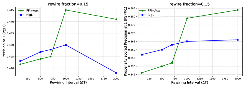
Figure 4: Effect of rewiring interval on final performance for Precision@1 (left) and propensity-scored Precision@1 (right) in the LF-AmazonTitles-131K dataset.

Table 4: Propensity-Scored Precision (PSP) comparison of our sparse model with its dense counterpart and state-of-the-art XMC methods on the Wiki10-31K, Wiki-500K, Amazon-670K, and Amazon-3M datasets. The same sparsity levels as mentioned in previous tables are used.

Method	PSP@1	PSP@3	PSP@5	PSP@1	PSP@3	PSP@5
	Wiki10-31K			Wiki-500K
AttentionXML	16.2	17.1	17.9	30.1	37.3	41.7
CascadeXML	13.2	14.7	16.1	31.3	39.4	43.3
Dense	10.6	12.6	13.9	32.5	41.0	44.9
Dense BN	12.4	14.5	16.0	28.5	36.5	40.1
Spartex	13.2	15.1	16.4	31.9	39.8	43.4
	Amazon-670K			Amazon-3M
AttentionXML	29.3	32.4	35.1	15.5	18.5	20.6
CascadeXML	30.2	34.9	38.8	-	-	-
Dense	33.3	36.9	39.9	15.6	19.0	21.5
Dense BN	26.9	30.9	34.5	13.5	16.4	18.6
Spartex	29.9	33.3	36.4	14.3	17.2	19.4

3.6 Performance on Tail Labels

Table 4 presents a comparison of Propensity-Scored Precision (PSP) for various Extreme Multi-label Classification (XMC) models, including AttentionXML You et al. (2019), CascadeXML Kharbanda et al. (2022), Dense, Dense Bottleneck, and our proposed method, across four benchmark datasets: Wiki10-31K, Wiki-500K, Amazon-670K, and Amazon-3M. For the Wiki10-31K dataset, our model achieves PSP@1 of 13.2, PSP@3 of 15.1, and PSP@5 of 16.4, surpassing the Dense model. On the Wiki-500K dataset, our method records a PSP@1 of 31.9, outperforming other XMC models and closely trailing the top-performing approaches. These findings underscore our model’s consistent performance across varied datasets, frequently exceeding or closely competing with XMC and Dense benchmarks. It’s noteworthy that the performance of AttentionXML on Wiki10-31K is attributed to its utilization of an LSTM encoder, which is particularly advantageous given the dataset’s smaller number of training samples relative to its label space. This configuration also explains our model’s superior performance compared to the Dense model, which incorporates a form of regularization. In comparisons involving memory efficiency, our approach significantly surpasses the same-capacity Dense Bottleneck model, demonstrating its suitability in resource-constrained settings where tail-label performance is critical.

Table 5: Comparison of Fan-in (sparsity) effects on model performance and memory usage for Amazon-670K dataset.

Fan in (sparsity)	Auxiliary Loss	P@1	P@3	P@5	$M_{\mathrm{tr}}$ $(\mathrm{GiB})$	Epoch Time (mins)	Inference Time (ms)
384 (50%)	No	49.0	43.5	39.5	7.03	18:13	10.2
384 (50%)	Yes	49.2	43.7	39.6	7.13	18:19	10.2
256 (67%)	No	47.0	41.6	37.7	5.27	15:45	9.18
256 (67%)	Yes	47.6	42.3	38.4	5.36	15:50	9.18
128 (83%)	No	45.6	40.2	36.3	3.60	13:20	8.54
128 (83%)	Yes	47.1	41.8	38.0	3.70	13:23	8.54
64 (92%)	No	30.7	26.5	23.6	2.88	12:12	8.14
64 (92%)	Yes	42.3	37.2	33.3	2.97	12:13	8.14
32 (96%)	No	5.5	5.0	4.6	2.52	11:36	7.94
32 (96%)	Yes	38.4	33.8	30.4	2.61	11:38	7.94

3.7 Impact of Varying Sparsity Levels

Table 5 illustrates the impact of varying sparsity levels (ranging from 50% to 96%) in conjunction with the use of auxiliary loss for Amazon-670K dataset. As sparsity levels increase, there are benefits in memory usage, training time, and inference time; however, performance metrics simultaneously decline. Additionally, the importance of auxiliary loss becomes particularly significant at higher sparsity levels.

3.8 Sensitivity to Auxiliary Loss cut-off epochs

We employ auxiliary loss with an initial scalar weight that decays until a specified cut-off epoch. Table 6 illustrates the model’s final performance at various cut-off epochs for two sparsity levels. A value of 0 (No aux) indicates the absence of auxiliary loss, while ’No cut-off’ signifies its application throughout training. Our analysis reveals that prolonging the auxiliary loss beyond optimal cut-off epochs adversely affects performance for both sparsity levels. Notably, maintaining the auxiliary loss throughout training leads to performance deterioration, resulting in scores lower than those achieved without its use.

Table 6: Comparison of Auxiliary loss cut-off epoch effects on model performance for different Fan-in (sparsity) levels.

Fan in: 128 (83% Sparsity)				Fan in: 64 (92% Sparsity)
Auxiliary cut-off epoch	P@1	P@3	P@5	Auxiliary cut-off epoch	P@1	P@3	P@5
0 (No aux)	45.6	40.2	36.3	0 (No aux)	30.7	26.5	23.6
15	47.1	41.8	38.0	15	42.3	37.2	33.3
30	46.6	41.1	37.1	30	32.8	28.3	25.2
60	45.9	40.6	36.6	60	32.5	28.0	24.9
90	44.6	39.7	35.9	90	31.3	27.0	23.9
No cut-off (full training)	42.1	37.4	33.7	No cut-off (full training)	22.7	17.7	14.4

3.9 DST with Fixed Embedding vs End-to-End Training

Table 7: Performance comparison between fixed CascadeXML Kharbanda et al. (2022) embeddings and end-to-end training with DST on Wiki-500K and Amazon-670K datasets.

	Wiki-500K			Amazon-670K
Method	P@1	P@3	P@5	P@1	P@3	P@5
Fixed	73.6	54.8	42.1	42.6	37.1	33.1
End-to-End	76.7	57.8	44.5	47.1	41.8	38.0

In Table 7, we compare the performance of models using fixed embeddings Schultheis and Babbar (2023) with trained end-to-end using DST on the Wiki-500K and Amazon-670K datasets. End-to-end training yields consistent improvements over fixed embeddings across all metrics, with significant gains in P@1 (an increase of 3.1% on Wiki-500K and 4.5% on Amazon-670K). These highlight the need of enabling the model to adapt its representations while training for the best possible performance.

4 Conclusion and future work

In this paper, we demonstrated the feasibility of DST for end-to-end training of classifiers with hundreds of thousands of labels. When appropriately adapted for XMC problems with fixed fan-in sparsity and an auxiliary objective, DST offers a significant reduction in peak memory usage while delivering superior performance compared to bottleneck-based weight reduction. It is anticipated that the Python bindings of the CUDA kernels will be useful for the research community in making their existing and forthcoming deep XMC pipelines more memory efficient. We hope that our work will enable further research towards developing techniques which could be (i) combined with explicit negative mining strategies, and (ii) used in conjunction with larger transformer encoders such as Roberta-large.

5 Limitations and societal impact

For XMC tasks, this paper attempts to explore the landscape of sparse neural networks, which can be trained on affordable and easily accessible commodity GPUs. While the proposed scheme is able to achieve comparable results to state-of-the-art methods at a fraction of GPU memory consumption, it is unable to surpass the baseline with dense last layer on all occasions. The exact relative decline in prediction performance, when our proposed adaptations of Fixed Fan-In and auxiliary objective are employed, is shown in Figure 3.

While we do not anticipate any negative societal impact of our work, it is expected that it will further enable the exploration of novel training methodologies for deep networks which are more affordable and easily accessible to a broader research community outside the big technology companies.

6 Acknowledgements

We thank Niki Loppi of NVIDIA AI Technology Center Finland for useful discussions on the sparse CUDA kernel implementations. YI acknowledges the support of Alberta Innovates (ALLRP-577350-22, ALLRP-222301502), the Natural Sciences and Engineering Research Council of Canada (RGPIN-2022-03120, DGECR-2022-00358), and Defence Research and Development Canada (DGDND-2022-03120). This research was enabled in part by support provided by the Digital Research Alliance of Canada (alliancecan.ca). RB acknowledges the support of Academy of Finland (Research Council of Finland) via grants 347707 and 348215. NU acknowledges the support of computational resources provided by the Aalto Science-IT project, and CSC IT Center for Science, Finland.

Appendix A Evaluation Metrics

To evaluate the performance of our Extreme Multi-label Text Classification (XMC) model, which incorporates Dynamic Sparse Training, we use a set of metrics designed to provide a comprehensive analysis of both overall and label-specific model performance. The primary metrics we employ is Precision at $k$ (P@$k$), which assess the accuracy of the top-$k$ predictions. Additionally, we incorporate Propensity-Scored Precision at $k$ (PSP@$k$), Macro Precision at $k$ (Macro P@$k$) and Macro Recall at $k$ (Macro R@$k$) to gauge the uniformity of the model’s effectiveness across the diverse range of labels typical in XMC problems.

Precision at $k$ (P@$k$):

Precision at k is the fundamental metric for evaluating the top-$k$ predictions in XMC applications such as e-commerce product recommendation and document tagging:

$$P@k(y,\hat{y})=\frac{1}{k}\sum_{\ell\in\text{top}_{k}(\hat{y})}y_{\ell}$$ (1)

where $y$ is the true label vector, $\hat{y}$ is the predicted score vector, and $\text{top}_{k}(\hat{y})$ identifies the indices with the top-$k$ highest predicted scores.

Propensity-Scored Precision at $k$ (PSP@$k$):

Given the long-tailed label distribution in many XMC datasets, PSP@k incorporates a propensity score $y_{l}$ to weight the precision contribution of each label, thereby emphasizing the tail labels’ performance:

$$PSP@k(y,\hat{y})=\frac{1}{k}\sum_{\ell\in\text{top}_{k}(\hat{y})}\frac{y_{\ell}}{p_{\ell}}$$ (2)

where $p_{l}$ corresponds to the propensity score for the label $y_{l}$ Jain et al. (2016).

Macro Precision at $k$ (Macro P@$k$):

To capture the average precision across all labels and mitigate any label imbalance, Macro Precision at $k$ is used:

$$\text{Macro }P@k=\frac{1}{L}\sum_{i=1}^{L}\left(\frac{\sum_{\ell\in\text{top}_{k}(\hat{y}_{i})}y_{i\ell}}{\min(k,\ |\text{top}_{k}(\hat{y}_{i})|)}\right)$$ (3)

Appendix B Baselines and Related Works

Despite the Dense and Same Capacity Dense baseline we also compare our approach with different State of the Art XMC methods and DST methods.

XMC Methods

We compare our method with deep XMC methods with mainly transformer encoder.

• AttentionXMLYou et al. (2019): The model segments labels using a shallow and wide PLT with a depth between 2 and 3, learning a specific context vector for each label to create label-adapted datapoint representations.

• LightXML Jiang et al. (2021): The method employs a transformer encoder to concurrently train both the retriever and ranker, which incorporates dynamic negative sampling to enhance the model’s efficacy.

• XR-Transformer Zhang et al. (2021): XR-Transformer employs a multi-resolution training approach, iteratively training and freezing the transformer before re-clustering and re-training classifiers at various resolutions using fixed features.

• CascadeXML Kharbanda et al. (2022): This method separates the feature learning of distinct tasks across various layers of the Probabilistic Label Tree (PLT) and aligns them with corresponding layers of the transformer encoder.

• ECLARE Mittal et al. (2021): This model utilizes label graphs to improve label representations, focusing specifically on enhancing performance for rare labels. The label graph is generated through random walks using the label vectors.

• SiameseXML Dahiya et al. (2021): This approach combines Siamese networks with one-vs-all classifiers. SiameseXML utilizes multiple ANNS structures to retrieve label shortlists. These shortlisted labels are subsequently ranked based on scores from label-wise one-vs-all classifiers.

• NGAME Dahiya et al. (2023): NGAME enhances transformer-based training for extreme classification by introducing a negative mining-aware mini-batching technique, which supports larger batch sizes and accelerates convergence by optimizing the handling of negative samples.

• Renee Jain et al. (2023): The Renee model employs an integrated end-to-end training approach for extreme classification, using a novel loss shortcut for memory optimization and a hybrid data-model parallel architecture to enhance training efficiency and scalability.

DST Methods

Existing DST methods vary in their pruning and growing criteria. Recent studies Nowak et al. (2024) indicate that magnitude-based pruning is effective in DST, while dense weight information is impractical for Extreme Multi-label Classification (XMC). We evaluate key methods on select datasets for conceptual validation.

• RigL Evci et al. (2020): RigL uses weight magnitude and dense gradient magnitudes for the pruning and regrowth saliency criteria, respectively. While RigL only needs the dense gradient information during network topology updates, this is a prohibitive requirement in the XMC setting due to the large memory consumption of the final classification layer. RigL learns an unstructured sparse network toplogy, which is challenging to accelerate on GPUs.

• Structured DST Lasby et al. (2024); Schultheis and Babbar (2023): In contrast to RigL, structured DST methods adds constraints to the learned network topology such that the network is more amenable to acceleration on commodity GPUs. In our case, we employ the fixed fan-in constraint which reduces both the latency and memory consumption of the final classification layer in the XMC setting. Further, since the dense gradient information is not available in the XMC task, we simply randomly regrow weights as per to SET (Mocanu et al., 2018) which has proven to be a robust baseline in the DST literature.

Appendix C Hyperparameter Settings

We present the hyperparameter settings used during training in Table 8. For the encoder and classifier, we employ two separate optimizers: AdamW for both components, except in the case of LF-AmazonTitles-131K where Adam and SGD are utilized. All experiments are conducted using half-precision float16 types, except for Amazon-3M and LF-AmazonTitles-131K, which use the bfloat16 type. We apply a cosine scheduler with warmup, as specified in the table. The weight decay values are set separately: 0.01 for the encoder and 1.0e-4 for the final classification layer. We use the squared hinge loss function for all datasets except for LF-AmazonTitles-131K, where we use binary cross-entropy (BCE) loss with positive labels.

Table 8: Hyperparameters of our approach to facilitate reproducibility. "LR" stands for learning rate.

Dataset	Encoder	Batch Size	Dropout	Epochs	LR Encoder	LR Classifier	Warmup	Sequence Length
Wiki10 31K	BERT Base	32	0.5	100	1.0e-5	0.01	1000	128
LF AmazonTtles 131K	Distil BERT	512	0.7	200	1.0e-5	0.08	5000	32
Wiki 500K	BERT Base	128	0.5	50	5.0e-5	0.05	1000	128
Amazon 670K	BERT Base	64	0.6	110	1.0e-5	0.01	1000	128
Amazon 3M	BERT Base	128	0.35	50	5.0e-5	0.05	10000	128

We also present DST and other related settings in a separate Table 9. The learning rates for the auxiliary classifier and the intermediate layer are fixed at 5.01e-4 and 2.01e-4, respectively. We use a random growth mode with zero initialization, updating the topology until 66% of the total training steps.

Table 9: DST and other related hyperparameter settings for different datasets.

Dataset	Fan-in (sparsity)	Prune mode	Rewire threshold	Rewire fraction	Rewire interval	Aux classifier	Aux cut-off	Inter. layer	Layer size
Wiki10 31K	64 (0.92)	fraction	-	0.25	300	No	-	Yes	4096
LF AmazonTitles 131K	128 (0.83)	fraction	-	0.15	1000	Yes	12	No	-
Wiki 500K	128 (0.83)	threshold	0.05	-	600	Yes	8	No	-
Amazon 670K	128 (0.83)	threshold	0.01	-	800	Yes	15	No	-
Amazon 3M	256 (0.67)	fraction	-	0.25	1500	Yes	8	No	-

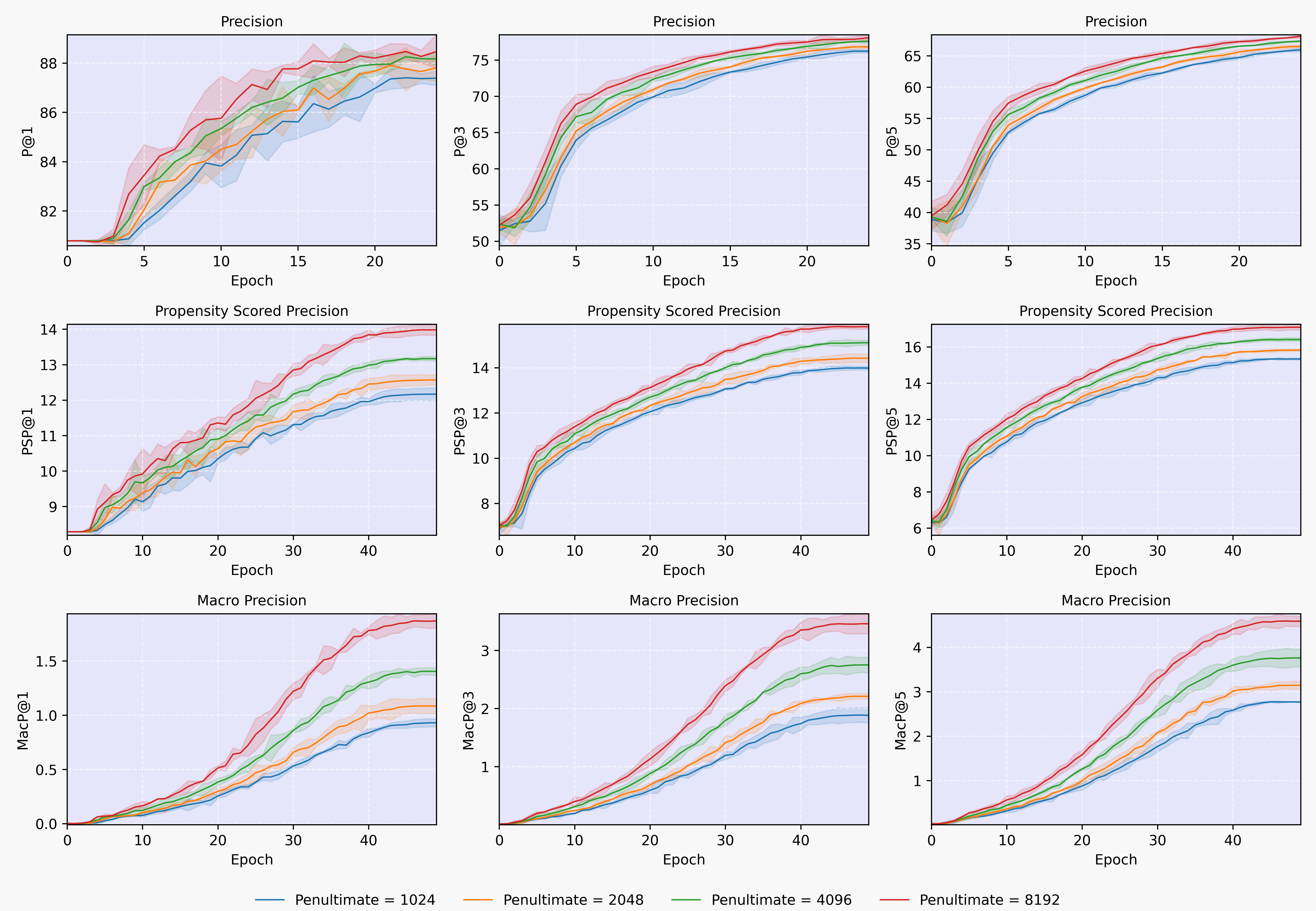
Figure 5: Impact of intermediate layer size on overall and tail label performance. The plots show precision, propensity-scored precision, and macro precision across epochs for different intermediate layer sizes (1024, 2048, 4096, and 8192).

Appendix D Effect of Intermediate Layer Size on Overall and Tail Label Performance

We investigated the impact of varying sizes of the intermediate layer on both overall performance and the performance of tail labels specifically as shown in Figure 5. It is important to highlight that although precision values peaked at certain layer sizes, the performance on tail labels continued to improve even beyond this point. This observation suggests that optimizing the size of the intermediate layer could play a crucial role in enhancing model effectiveness, particularly for tail labels which are often more challenging to predict accurately.

Appendix E The Role of Random Cluster based Meta Classifiers in XMC Problems

To understand the impact of random clusters on meta classifier-based methods, we selected the LightXML Jiang et al. (2021) approach and experimented with two large-scale datasets: Amazon-670K and Wiki-500K. For our experiments, we used the original code from the official LightXML repository and the original clusters provided by the authors. We randomized the original clusters by applying several iterations of random.shuffle(), repeating the process twice to generate two sets of random clusters.

To ensure randomness, we calculated the intersection of elements between each pair of clusters from the original and random sets. We then took the maximum overlap value among all pairs, which was less than $3.5\%$ in both cases. Subsequently, we ran the LightXML code using the original clusters and the two sets of random clusters.

Our observations revealed that the final performance remained largely unaffected, although the learning process slowed down initially, as shown in the upper row of Figure 6. The bottom row illustrates the precision of the meta classifier, which is lower for the random clusters as expected. We replicated the same experiment with the Wiki-500K dataset and observed similar results, which are also depicted in Figure 7.

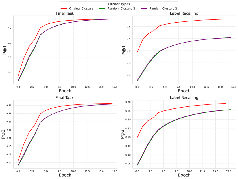
Figure 6: Final task and meta level precision performance for Amazon-670K

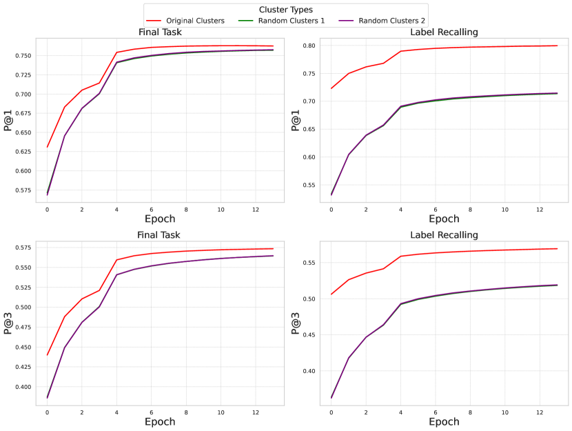
Figure 7: Final task and meta level precision performance for Wiki-500K

Appendix F Computational Resources

While we want to demonstrate the memory efficiency of our algorithms, in order to enable meaningful comparison with existing methods, we run all our experiments on a NVidia A100 GPU, and measure the memory consumption using torch.cuda.max_memory_allocated. On this GPU, the experiments with Wiki31K take about 1 hour, Amazon-131K 8 hours, Amazon-670k 30 hours, Wikipedia-500k 36 hours and Amazon-3M 72 hours.

References

- Frankle and Carbin [2018] Jonathan Frankle and Michael Carbin. The lottery ticket hypothesis: Finding sparse, trainable neural networks. In International Conference on Learning Representations, 2018.
- Frankle et al. [2020] Jonathan Frankle, Gintare Karolina Dziugaite, Daniel Roy, and Michael Carbin. Linear mode connectivity and the lottery ticket hypothesis. In International Conference on Machine Learning, pages 3259–3269. PMLR, 2020.
- Malach et al. [2020] Eran Malach, Gilad Yehudai, Shai Shalev-Schwartz, and Ohad Shamir. Proving the lottery ticket hypothesis: Pruning is all you need. In International Conference on Machine Learning, pages 6682–6691. PMLR, 2020.
- Chen et al. [2021a] Tianlong Chen, Jonathan Frankle, Shiyu Chang, Sijia Liu, Yang Zhang, Michael Carbin, and Zhangyang Wang. The lottery tickets hypothesis for supervised and self-supervised pre-training in computer vision models. In Proceedings of the IEEE/CVF conference on computer vision and pattern recognition, pages 16306–16316, 2021a.
- Mocanu et al. [2018] Decebal Constantin Mocanu, Elena Mocanu, Peter Stone, Phuong H Nguyen, Madeleine Gibescu, and Antonio Liotta. Scalable training of artificial neural networks with adaptive sparse connectivity inspired by network science. Nature communications, 9(1):2383, 2018.
- Evci et al. [2020] Utku Evci, Trevor Gale, Jacob Menick, Pablo Samuel Castro, and Erich Elsen. Rigging the lottery: Making all tickets winners. In International conference on machine learning, pages 2943–2952. PMLR, 2020.
- Liu et al. [2021a] Shiwei Liu, Lu Yin, Decebal Constantin Mocanu, and Mykola Pechenizkiy. Do we actually need dense over-parameterization? in-time over-parameterization in sparse training. In International Conference on Machine Learning, pages 6989–7000. PMLR, 2021a.
- Dietrich et al. [2021] Anastasia Dietrich, Frithjof Gressmann, Douglas Orr, Ivan Chelombiev, Daniel Justus, and Carlo Luschi. Towards structured dynamic sparse pre-training of bert. arXiv preprint arXiv:2108.06277, 2021.
- Liu et al. [2021b] Shiwei Liu, Iftitahu Ni’mah, Vlado Menkovski, Decebal Constantin Mocanu, and Mykola Pechenizkiy. Efficient and effective training of sparse recurrent neural networks. Neural Computing and Applications, 33:9625–9636, 2021b.
- Tan et al. [2022] Yiqin Tan, Pihe Hu, Ling Pan, Jiatai Huang, and Longbo Huang. Rlx2: Training a sparse deep reinforcement learning model from scratch. In The Eleventh International Conference on Learning Representations, 2022.
- Graesser et al. [2022] Laura Graesser, Utku Evci, Erich Elsen, and Pablo Samuel Castro. The state of sparse training in deep reinforcement learning. In International Conference on Machine Learning, pages 7766–7792. PMLR, 2022.
- Guo et al. [2018] Yiwen Guo, Chao Zhang, Changshui Zhang, and Yurong Chen. Sparse dnns with improved adversarial robustness. Advances in neural information processing systems, 31, 2018.
- Özdenizci and Legenstein [2021] Ozan Özdenizci and Robert Legenstein. Training adversarially robust sparse networks via bayesian connectivity sampling. In International Conference on Machine Learning, pages 8314–8324. PMLR, 2021.
- Chen et al. [2021b] Tianlong Chen, Zhenyu Zhang, Santosh Balachandra, Haoyu Ma, Zehao Wang, Zhangyang Wang, et al. Sparsity winning twice: Better robust generalization from more efficient training. In International Conference on Learning Representations, 2021b.
- Diffenderfer et al. [2021] James Diffenderfer, Brian Bartoldson, Shreya Chaganti, Jize Zhang, and Bhavya Kailkhura. A winning hand: Compressing deep networks can improve out-of-distribution robustness. Advances in neural information processing systems, 34:664–676, 2021.
- Liu et al. [2022] Shiwei Liu, Tianlong Chen, Zahra Atashgahi, Xiaohan Chen, Ghada Sokar, Elena Mocanu, Mykola Pechenizkiy, Zhangyang Wang, and Decebal Constantin Mocanu. Deep ensembling with no overhead for either training or testing: The all-round blessings of dynamic sparsity. In 10th International Conference on Learning Representations, ICLR 2022. OpenReview, 2022.
- Evci et al. [2022] Utku Evci, Yani Ioannou, Cem Keskin, and Yann Dauphin. Gradient flow in sparse neural networks and how lottery tickets win. In Proceedings of the AAAI conference on artificial intelligence, volume 36, pages 6577–6586, 2022.
- Price and Tanner [2021] Ilan Price and Jared Tanner. Dense for the price of sparse: Improved performance of sparsely initialized networks via a subspace offset. In International Conference on Machine Learning, pages 8620–8629. PMLR, 2021.
- Curci et al. [2021] Selima Curci, Decebal Constantin Mocanu, and Mykola Pechenizkiyi. Truly sparse neural networks at scale. arXiv preprint arXiv:2102.01732, 2021.
- Bhatia et al. [2016] K. Bhatia, K. Dahiya, H. Jain, P. Kar, A. Mittal, Y. Prabhu, and M. Varma. The extreme classification repository: Multi-label datasets and code, 2016. URL http://manikvarma.org/downloads/XC/XMLRepository.html.
- Babbar and Schölkopf [2017] Rohit Babbar and Bernhard Schölkopf. Dismec: Distributed sparse machines for extreme multi-label classification. In Proceedings of the tenth ACM international conference on web search and data mining, pages 721–729, 2017.
- Prabhu et al. [2018] Yashoteja Prabhu, Anil Kag, Shrutendra Harsola, Rahul Agrawal, and Manik Varma. Parabel: Partitioned label trees for extreme classification with application to dynamic search advertising. In Proceedings of the 2018 World Wide Web Conference, pages 993–1002, 2018.
- Jiang et al. [2021] Ting Jiang, Deqing Wang, Leilei Sun, Huayi Yang, Zhengyang Zhao, and Fuzhen Zhuang. Lightxml: Transformer with dynamic negative sampling for high-performance extreme multi-label text classification. In Proceedings of the AAAI conference on artificial intelligence, volume 35, pages 7987–7994, 2021.
- You et al. [2019] Ronghui You, Zihan Zhang, Ziye Wang, Suyang Dai, Hiroshi Mamitsuka, and Shanfeng Zhu. Attentionxml: Label tree-based attention-aware deep model for high-performance extreme multi-label text classification. Advances in neural information processing systems, 32, 2019.
- Kharbanda et al. [2022] Siddhant Kharbanda, Atmadeep Banerjee, Erik Schultheis, and Rohit Babbar. Cascadexml: Rethinking transformers for end-to-end multi-resolution training in extreme multi-label classification. Advances in neural information processing systems, 35:2074–2087, 2022.
- Dahiya et al. [2021] Kunal Dahiya, Ananye Agarwal, Deepak Saini, K Gururaj, Jian Jiao, Amit Singh, Sumeet Agarwal, Purushottam Kar, and Manik Varma. Siamesexml: Siamese networks meet extreme classifiers with 100m labels. In International conference on machine learning, pages 2330–2340. PMLR, 2021.
- Dahiya et al. [2023] Kunal Dahiya, Nilesh Gupta, Deepak Saini, Akshay Soni, Yajun Wang, Kushal Dave, Jian Jiao, Gururaj K, Prasenjit Dey, Amit Singh, et al. Ngame: Negative mining-aware mini-batching for extreme classification. In Proceedings of the Sixteenth ACM International Conference on Web Search and Data Mining, pages 258–266, 2023.
- Zhang et al. [2021] Jiong Zhang, Wei-Cheng Chang, Hsiang-Fu Yu, and Inderjit Dhillon. Fast multi-resolution transformer fine-tuning for extreme multi-label text classification. Advances in Neural Information Processing Systems, 34:7267–7280, 2021.
- Schultheis and Babbar [2022] Erik Schultheis and Rohit Babbar. Speeding-up one-versus-all training for extreme classification via mean-separating initialization. Machine Learning, 111(11):3953–3976, 2022.
- Qaraei and Babbar [2024] Mohammadreza Qaraei and Rohit Babbar. Meta-classifier free negative sampling for extreme multilabel classification. Machine Learning, 113(2):675–697, 2024.
- Babbar and Schölkopf [2019] Rohit Babbar and Bernhard Schölkopf. Data scarcity, robustness and extreme multi-label classification. Machine Learning, 108(8):1329–1351, 2019.
- Yen et al. [2016] Ian En-Hsu Yen, Xiangru Huang, Pradeep Ravikumar, Kai Zhong, and Inderjit Dhillon. Pd-sparse: A primal and dual sparse approach to extreme multiclass and multilabel classification. In International conference on machine learning, pages 3069–3077. PMLR, 2016.
- Medini et al. [2019] Tharun Kumar Reddy Medini, Qixuan Huang, Yiqiu Wang, Vijai Mohan, and Anshumali Shrivastava. Extreme classification in log memory using count-min sketch: A case study of amazon search with 50m products. Advances in Neural Information Processing Systems, 32, 2019.
- Schultheis and Babbar [2023] Erik Schultheis and Rohit Babbar. Towards memory-efficient training for extremely large output spaces–learning with 670k labels on a single commodity gpu. In Joint European Conference on Machine Learning and Knowledge Discovery in Databases, pages 689–704. Springer, 2023.
- Jain et al. [2023] Vidit Jain, Jatin Prakash, Deepak Saini, Jian Jiao, Ramachandran Ramjee, and Manik Varma. Renee: End-to-end training of extreme classification models. Proceedings of Machine Learning and Systems, 5, 2023.
- Liu et al. [2023] Shiwei Liu, Tianlong Chen, Zhenyu Zhang, Xuxi Chen, Tianjin Huang, Ajay Jaiswal, and Zhangyang Wang. Sparsity may cry: Let us fail (current) sparse neural networks together! arXiv preprint arXiv:2303.02141, 2023.
- Jaiswal et al. [2024] Ajay Kumar Jaiswal, Zhe Gan, Xianzhi Du, Bowen Zhang, Zhangyang Wang, and Yinfei Yang. Compressing LLMs: The truth is rarely pure and never simple. In The Twelfth International Conference on Learning Representations, 2024.
- Jain et al. [2016] Himanshu Jain, Yashoteja Prabhu, and Manik Varma. Extreme multi-label loss functions for recommendation, tagging, ranking & other missing label applications. In Proceedings of the 22nd ACM SIGKDD international conference on knowledge discovery and data mining, pages 935–944, 2016.
- Buvanesh et al. [2023] Anirudh Buvanesh, Rahul Chand, Jatin Prakash, Bhawna Paliwal, Mudit Dhawan, Neelabh Madan, Deepesh Hada, Vidit Jain, SONU MEHTA, Yashoteja Prabhu, et al. Enhancing tail performance in extreme classifiers by label variance reduction. In The Twelfth International Conference on Learning Representations, 2023.
- Schultheis et al. [2024] Erik Schultheis, Marek Wydmuch, Wojciech Kotlowski, Rohit Babbar, and Krzysztof Dembczynski. Generalized test utilities for long-tail performance in extreme multi-label classification. Advances in Neural Information Processing Systems, 36, 2024.
- Qaraei et al. [2021] Mohammadreza Qaraei, Erik Schultheis, Priyanshu Gupta, and Rohit Babbar. Convex surrogates for unbiased loss functions in extreme classification with missing labels. In Proceedings of the Web Conference 2021, pages 3711–3720, 2021.
- Schultheis et al. [2022] Erik Schultheis, Marek Wydmuch, Rohit Babbar, and Krzysztof Dembczynski. On missing labels, long-tails and propensities in extreme multi-label classification. In Proceedings of the 28th ACM SIGKDD Conference on Knowledge Discovery and Data Mining, pages 1547–1557, 2022.
- Schultheis and Babbar [2021] Erik Schultheis and Rohit Babbar. Unbiased loss functions for multilabel classification with missing labels. arXiv preprint arXiv:2109.11282, 2021.
- Devlin et al. [2018] Jacob Devlin, Ming-Wei Chang, Kenton Lee, and Kristina Toutanova. Bert: Pre-training of deep bidirectional transformers for language understanding. arXiv preprint arXiv:1810.04805, 2018.
- Sanh [2019] V Sanh. Distilbert, a distilled version of bert: smaller, faster, cheaper and lighter. In Proceedings of Thirty-third Conference on Neural Information Processing Systems (NIPS2019), 2019.
- Lasby et al. [2024] Mike Lasby, Anna Golubeva, Utku Evci, Mihai Nica, and Yani Ioannou. Dynamic sparse training with structured sparsity. In The Twelfth International Conference on Learning Representations, 2024.
- McAuley and Leskovec [2013] Julian McAuley and Jure Leskovec. Hidden factors and hidden topics: understanding rating dimensions with review text. In Proceedings of the 7th ACM conference on Recommender systems, pages 165–172, 2013.
- Mittal et al. [2021] Anshul Mittal, Noveen Sachdeva, Sheshansh Agrawal, Sumeet Agarwal, Purushottam Kar, and Manik Varma. Eclare: Extreme classification with label graph correlations. In Proceedings of the Web Conference 2021, pages 3721–3732, 2021.
- Vaswani et al. [2017] Ashish Vaswani, Noam Shazeer, Niki Parmar, Jakob Uszkoreit, Llion Jones, Aidan N Gomez, Łukasz Kaiser, and Illia Polosukhin. Attention is all you need. Advances in neural information processing systems, 30, 2017.
- Kurtic et al. [2024] Eldar Kurtic, Torsten Hoefler, and Dan Alistarh. How to prune your language model: Recovering accuracy on the “sparsity may cry” benchmark. In Conference on Parsimony and Learning, pages 542–553. PMLR, 2024.
- Hoefler et al. [2021] Torsten Hoefler, Dan Alistarh, Tal Ben-Nun, Nikoli Dryden, and Alexandra Peste. Sparsity in deep learning: Pruning and growth for efficient inference and training in neural networks. Journal of Machine Learning Research, 22(241):1–124, 2021.
- Hassibi and Stork [1992] Babak Hassibi and David Stork. Second order derivatives for network pruning: Optimal brain surgeon. Advances in neural information processing systems, 5, 1992.
- Dai et al. [2019] Xiaoliang Dai, Hongxu Yin, and Niraj K Jha. Nest: A neural network synthesis tool based on a grow-and-prune paradigm. IEEE Transactions on Computers, 68(10):1487–1497, 2019.
- Dettmers and Zettlemoyer [2019] Tim Dettmers and Luke Zettlemoyer. Sparse networks from scratch: Faster training without losing performance. arXiv preprint arXiv:1907.04840, 2019.
- Lin et al. [2020] Tao Lin, Sebastian U. Stich, Luis Barba, Daniil Dmitriev, and Martin Jaggi. Dynamic model pruning with feedback. In International Conference on Learning Representations, 2020. URL https://openreview.net/forum?id=SJem8lSFwB.
- Nowak et al. [2024] Aleksandra Nowak, Bram Grooten, Decebal Constantin Mocanu, and Jacek Tabor. Fantastic weights and how to find them: Where to prune in dynamic sparse training. Advances in Neural Information Processing Systems, 36, 2024.
- Gale et al. [2020] Trevor Gale, Matei Zaharia, Cliff Young, and Erich Elsen. Sparse gpu kernels for deep learning. In SC20: International Conference for High Performance Computing, Networking, Storage and Analysis, pages 1–14. IEEE, 2020.
- Lee et al. [2023] Joo Hyung Lee, Wonpyo Park, Nicole Elyse Mitchell, Jonathan Pilault, Johan Samir Obando Ceron, Han-Byul Kim, Namhoon Lee, Elias Frantar, Yun Long, Amir Yazdanbakhsh, Woohyun Han, Shivani Agrawal, Suvinay Subramanian, Xin Wang, Sheng-Chun Kao, Xingyao Zhang, Trevor Gale, Aart J.C. Bik, Milen Ferev, Zhonglin Han, Hong-Seok Kim, Yann Dauphin, Gintare Karolina Dziugaite, Pablo Samuel Castro, and Utku Evci. Jaxpruner: A concise library for sparsity research. In Conference on Parsimony and Learning (Proceedings Track), 2023. URL https://openreview.net/forum?id=H2rCZCfXkS.
- Castro et al. [2023] Roberto L Castro, Andrei Ivanov, Diego Andrade, Tal Ben-Nun, Basilio B Fraguela, and Torsten Hoefler. Venom: A vectorized n: M format for unleashing the power of sparse tensor cores. In Proceedings of the International Conference for High Performance Computing, Networking, Storage and Analysis, pages 1–14, 2023.
- Mishra et al. [2021] Asit Mishra, Jorge Albericio Latorre, Jeff Pool, Darko Stosic, Dusan Stosic, Ganesh Venkatesh, Chong Yu, and Paulius Micikevicius. Accelerating sparse deep neural networks. arXiv preprint arXiv:2104.08378, 2021.
- Liu and Wang [2023] Shiwei Liu and Zhangyang Wang. Ten lessons we have learned in the new "sparseland": A short handbook for sparse neural network researchers, 2023. URL https://arxiv.org/abs/2302.02596.
- Micikevicius et al. [2018] Paulius Micikevicius, Sharan Narang, Jonah Alben, Gregory Diamos, Erich Elsen, David Garcia, Boris Ginsburg, Michael Houston, Oleksii Kuchaiev, Ganesh Venkatesh, et al. Mixed precision training. In International Conference on Learning Representations, 2018.
- Chen et al. [2016] Tianqi Chen, Bing Xu, Chiyuan Zhang, and Carlos Guestrin. Training deep nets with sublinear memory cost. arXiv preprint arXiv:1604.06174, 2016.
- Kharbanda et al. [2023] Siddhant Kharbanda, Atmadeep Banerjee, Devaansh Gupta, Akash Palrecha, and Rohit Babbar. Inceptionxml: A lightweight framework with synchronized negative sampling for short text extreme classification. In Proceedings of the 46th International ACM SIGIR Conference on Research and Development in Information Retrieval, pages 760–769, 2023.
- Zubiaga [2012] Arkaitz Zubiaga. Enhancing navigation on wikipedia with social tags. arXiv preprint arXiv:1202.5469, 2012.
- McAuley et al. [2015] Julian McAuley, Rahul Pandey, and Jure Leskovec. Inferring networks of substitutable and complementary products. In Proceedings of the 21th ACM SIGKDD international conference on knowledge discovery and data mining, pages 785–794, 2015.
- Liu [2019] Yinhan Liu. Roberta: A robustly optimized bert pretraining approach. arXiv preprint arXiv:1907.11692, 364, 2019.