A comparison of solar and stellar coronagraphs that make use of external occulters

Abstract

Solar and stellar externally occulted coronagraphs share similar concepts, but are actually very different because of geometric characteristics. Solar occulters were first developed with a simple geometric model of diffraction perpendicular to the occulter edges. We apply this mere approach to starshades, and introduce a simple shifted circular integral of the occulter which allows to illustrate the influence of the number of petals on the extent of the deep central dark zone. We illustrate the reasons for the presence of an internal coronagraph in the solar case and its absence in the exoplanet case.

1 INTRODUCTION

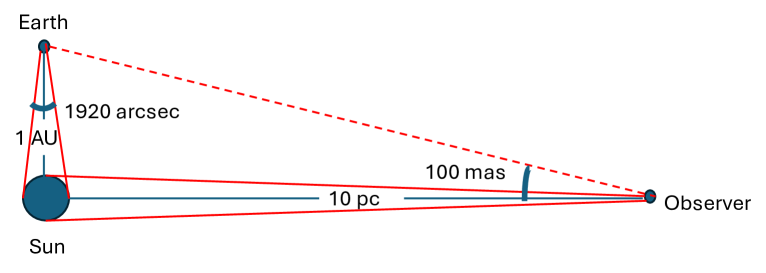
Figure 1: Illustration of characteristic dimensions for solar and stellar coronagraphs. Distances are from 1 AU to 10 pc.

Astronomical objectives for solar and stellar coronagraphs are the study of the solar corona and the detection of exoplanets. We consider here coronagraphs using external occulters on the model of the occultation of the Sun by the Moon. These coronagraphs share similar concepts but become different because of geometric characteristics. In round numbers, distances between the objects to be occulted by these coronagraphs are as 1 astronomical unit (AU) for the solar corona vs 10 parsecs or more for exoplanets, a factor of 2 million or so. A very schematic comparative representation of the observational parameters is given in Fig. 1 and a list of experimental parameters is given in Table 1. From a near-Earth orbit, the Sun is seen at an angle of about half a degree. We seek to see the solar corona as close as possible to the solar disk, and the external occulter is just greater than the apparent diameter of the solar photosphere. The corona is observed over a few solar radii. For exoplanets, considering an extra-solar system at 10 parsecs, the angle between the exo-Sun and the exo-Earth is 100 milliarcsec, and the stellar diameter would be seen at an angle of 1 mas. Starshades, with all the experimental constraints, do not have the possibility to just obscure the 1 mas star, and consider much larger obstruction angles, 50 to 100 times as large, just to allow the detection of an exo-Earth. A heuristic and historical presentation of the ideas leading to the diversity of external solar occulters is made in Section 2. A similar presentation for exoplanets is given in Section 3, which gives the opportunity to introduce a function which can be considered as a shifted apodization profile. An empirical justification of the usefulness of an internal coronagraph in the solar case and its low efficiency in the case of exoplanets is given in Section 4.

Table 1: Comparison between solar and stellar coronagraphs. In addition to the orders of magnitude between dimensions, a main point is that the solar disk is a huge extended object versus the almost point source star. Values are for a typical extra-solar system seen at 10 parsecs.

Science object	Solar Corona	Exoplanets
Occulter diameters	A few cm. to 1.5 m.	10 m. to 100 m.
Occulter shapes	Single or multiple discs, Serrated, Multithreaded …	Petal-shaped
Occulter telescope distance	A few cm., up to 150 m	10 to 100 $\times 10^{6}$ m.
Telescope diameter	A few cm., up to 5cm	1 m. to 6.5 m.
Straylight origin	Solar photosphere	The star
Type of source	Very extended (1920 arcsecs)	Point-like (1 mas)
Linear res. pixels in the source	1000	0.01
IWA/$\Phi$ source	1 - 1.03	30 - 70
Field of view	A few degrees	1 arcsec
Required rejection	$10^{-6}-10^{-9}$	$10^{-6}-10^{-12}$
Internal coronagraph	Lyot type	No
Fresnel number	$10^{2}-10^{4}$	1 - 10

2 SOLAR EXTERNAL OCCULTERS

The use of external occulters to shade the bright solar photosphere to observe the faint solar corona without natural eclipses has a long history. Solar astronomers considered first that Lyot’s coronagraph [1], with the rather low quality of optical systems of their time, cannot be improved enough to observe the outer corona [2, 3]. Then, with reference to Evans’s photometer [4], an external occulter is set in front of the Lyot coronagraph in almost all space-born coronagraphs, as described by Koutchmy [5]. In overall, the effects of the external occulter provide the same rejection rate as that of the Lyot coronagraph, and these effects multiply.

Observers were very inventive. In 1963, Tousey [6], used a serrated-edge external-occulter and obtained the first observations of the outer solar corona in the absence of an eclipse. Purcell and Koomen [7] proposed to use a system of multiple circular disks. A decisive step was made with the coronagraph SOHO/LASCO [8], in operation since 1995. In their experimental study of new generations of external occulters for LASCO-C2, they [9] found that conic occulters gave performances superior to multiple discs occulters.

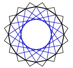
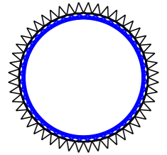
Figure 2: Illustration of the Boivin radius $R\cos(\alpha)$ as the envelop of rays perpendicular to the edges of the teeth. The angle $\alpha$ must be as small as possible so that the Boivin radius approaches that of the central disk, which requires a very large number of short teeth not to mask the inner corona.

The idea that leads to serrated external occulters for solar astronomy is of geometric origin. It is assumed that wave diffraction occurs over planes perpendicular to the edges of the screen. Triangular teeth are placed on the edge of the circular occulters to move light away from the center of the optical axis. Boivin [10] shown that a dark disk of radius $R\cos(\alpha)$ is sheltered from the rays diffracted by the edges, where $R$ is the occulter radius and $\alpha$ is the exterior angle of the half-teeth triangle as shown in the right drawing of Fig.2. This effect was recently numerically verified using the Maggi-Rubinowicz boundary integral [11]. Serrated occulters are a simplified version of petal occulters. A gain of several orders of magnitude in rejection could be obtained if the triangular teeth would be replaced by a petal having a more studied shape, for example a Sonine function [12], but no experiment of this type is currently envisaged.

The use of several disk occulters followed another reasoning. The idea is that the Arago spot exists because the edge of the circular occulter seen from the telescope is bright. The solution found by solar astronomers of the sixteen is to darken this edge. Tousay [6] considered that the best arrangement was a system of several discs, so that each disk casts a shadow on the edge of the next disk. Fig.3 gives an illustration for 2 discs at the distances $z$ and $d$ of the entrance aperture. The second disc of diameter $\omega$ must be in the shadow of the first disc of diameter $\Omega$, with the mandatory requirement that from the telescope the first disc is not visible, so that $\Omega>\omega>d/z\Omega$. Analytical expressions exist for 2 and 3 disks but are difficult to evaluate numerically. We can generalize these calculations to more disks and obtain the ideal shape for a multi-disk occulter by continuity [13]. The exact calculation of the Fresnel diffraction of a true 3D occulter has not been carried out, to the limit of knowledge of the authors of this paper.

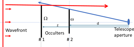
Figure 3: Left, principle diagram: two disks $\#1$ and $\#2$ of diameters $\Omega$ and $\omega$ are at distances $z$ and $d$ from the entrance aperture of the telescope. Right: a substantial light reduction is obtained provided that $\omega$ is half-way between the conditions $\omega\leq\Omega$ and $\omega\geq d/z\Omega$.

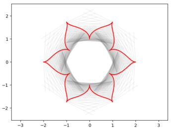
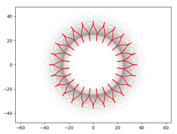
Figure 4: Illustration with the approach of Boivin using rays diffracting perpendicular to the edges of the petals for an occulter with 6 petals for which the profile is a mere cosine arch (left) and an occulter with 24 petals (right) corresponding to NW2 of SISTER which gives off a larger circular dark central area.

3 Stellar external occulters (Starshade)

For stellar external occulters, the prevailing philosophy is to define an optimal apodized transmission [14] which makes it possible to obtain a very dark central zone with an intensity less than $10^{-10}$ allowing to see exoplanets [15], using the smallest possible shaped-occulter [16],[17], [18]. Considering that these immense occulters cannot be manufactured with variable transmission, shaped occulters [19] are used as the alternative to produce the central black zone. Figure 4 shows an illustration of Boivin’s empirical approach to these petal occulters. Here also as for the solar serrated occulter case, a dark central zone sheltered from the rays diffracting perpendicular to the edges of the petals is evidenced. A 24-petal occulter with a very studied profile is clearly more effective than a 6-petal occulter with a simpler profile.

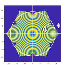
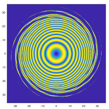
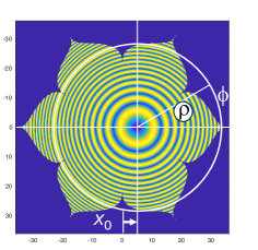
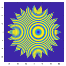
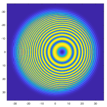
Figure 5: The function $g(\rho,X_{0})$ of Eq.3 corresponds to the mean value along concentric circles centered at $x=X_{0}$ of the occulter transmission. In these figures, an illustration of the quadratic phase of Eq.2 is given behind. Top panels are for $X_{0}=0$. The two left occulters correspond to the same value $g(\rho,0)=p(\rho)$ that the apodized occulter at right, and therefore the same complex amplitude $\Psi(0,0)$ at the center of the Fresnel diffraction pattern. Bottom panels are for $X_{0}=5$ m, 6-petals and 24-petals occulters and the apodized one. A drawing of $g(\rho,X_{0})$ for different $X_{0}$ values is given in Fig.6.

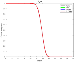
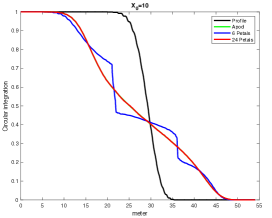
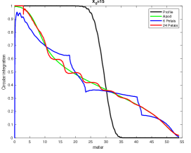
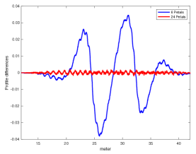
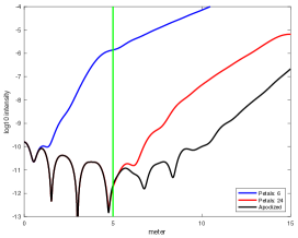
Figure 6: Top panels, the functions $g(\rho,X_{0})$, for apodized, 6-petals and 24-petals occulters, for $X_{0}=$0, 10 and 15m. As expected all functions merge with the profile $p(\rho)$ of NW2 of SISTER[20] for $X_{0}=0$. Bottom panels correspond to the illustration $X_{0}=5$m given in Fig. 5. Left, the functions $g(\rho,5)$, center, the differences $g_{6}(\rho,5)-g_{a}(\rho,5)$ and $g_{24}(\rho,5)-g_{a}(\rho,5)$, and right the intensity diffraction patterns (log10 scale) for the apodized, 6-petals and 24-petals occulters computed using the model of Vanderbei et al.[16]. The vertical green line is at the position $X_{0}=5$m from center.

For a more detailed analysis of the effects of the number of petals, consider the equation giving the Fresnel diffraction of an occulter $f(x,y)$ at the distance $z$ and at the wavelength $\lambda$ in the form of a convolution product:

$$\Psi(x,y)=1-f(x,y)*\frac{1}{i\lambda z}\exp(i\pi\frac{x^{2}+y^{2}}{\lambda z}).$$ (1)

For $x=X_{0},y=0$, this convolution can be written as:

$$\Psi(X_{0},0)=1-\frac{1}{i\lambda z}\int\int\exp(i\pi\frac{\xi^{2}+\eta^{2}}{\lambda z})f(X_{0}-\xi,0-\eta)d\xi d\eta=1-\frac{2\pi}{i\lambda z}\int g(\rho,X_{0})\exp(i\pi\frac{\rho^{2}}{\lambda z})\rho^{2}d\rho$$ (2)

where a change of Cartesian to radial coordinates was made to introduce the function

$$g(\rho,X_{0})=\frac{1}{2\pi\rho}\int_{0}^{2\pi}f(\rho\cos(\phi)+X_{0},\rho\sin(\phi))d\phi$$ (3)

that is the integral of the occulter $f(x,y)$ along concentric circles centered at the point $(X_{0},0)$, taken as the new origin of the axes. An illustration of the integration is given in Fig. 5. The result of the integral is finally divided by $2\pi\rho$ to obtain the average transmission on the circles.

For $X_{0}=0$, the petal-occulters are constructed such that $g(\rho,0)=p(\rho)$, the optimal apodized transmission [15]. In other words, the average of the all-or-nothing petal transmissions (1 or 0) on the concentric circles recovers the ideal variable transmission, here the profile NW2[20], which cannot be physically realized otherwise. The three occulters of the top panels of Fig. 5, the 6-petals occulter (left), a spiral version of it obtained using a twist of the petals (middle), complete the request and give the same mean circularly integrated value that the apodized occulter (right). Many shaped occulters may fit this requirement.

The $X_{0}\neq 0$ case is illustrated in the bottom panels of Fig. 5 for $X_{0}=5$m. There we have considered the integrals for a 6-petals and a 24-petals occulter, and for the apodized occulter of NW2. The circular averages are then all different.

An illustration of $g(\rho,X_{0})$ for $X_{0}=0,5,10$ and 15 m is given in Fig.6 for the 6 and 24 shaped occulters $g_{6}(\rho,5),g_{24}(\rho,5)$ and the apodized occulter $g_{a}(\rho,5)$. As a reference $p(\rho)$ is drawn in these figures. The function $g(\rho,X_{0})$ departs from $p(\rho)$, and spread out as $X_{0}$ increases. The calculations are made in the direction of a tip of the petals, the curves are different in the direction of a hollow, but without changing the conclusion for the comparison between occulters. It appears in any case that $g_{24}(\rho,X_{0})$ is much closer to $g_{a}(\rho,X_{0})$ than $g_{6}(\rho,X_{0})$, and so are the diffraction patterns as expected by the theory of Vanderbei et al.[16]. This is well evidenced by differences between curves. We can consider a priory that the best shaped occulter is the one whose function $g(\rho,X_{0})$ is as close as possible to $g_{a}(\rho,X_{0})$.

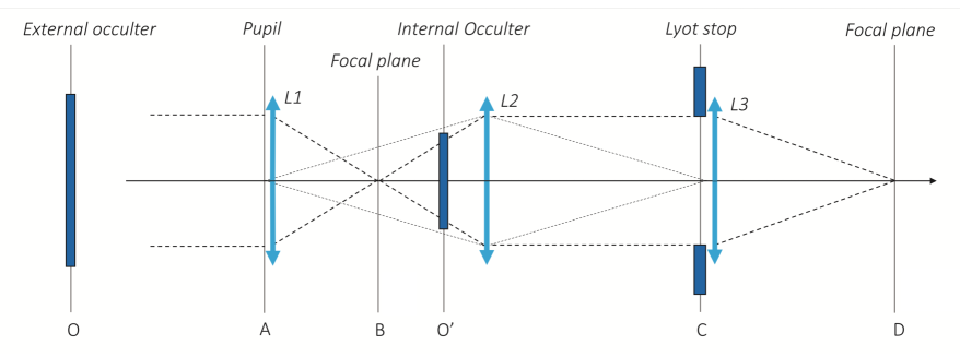
Figure 7: Schematic diagram of a Lyot coronagraph coupled to an external occulter. Planes A, B, C, D are the classic planes of the Lyot coronagraph. The Lyot mask is in plane B, the Lyot stop in plane D. The presence of the external occulter (O) modifies the device such that the internal occulter must be optimally placed on the image (O’) of the occulter. For exoplanets, we cannot differentiate O’ from B.

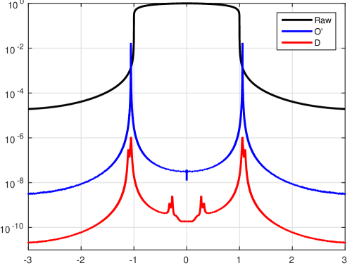
Figure 8: Illustration of the effect of the Lyot coronagraph on the rejection of stray light for the ASPIICS solar coronagraph[21]. The black curve is the direct image of the solar photosphere (plane B) with a straylight at $10^{-4}$, the blue curve gives the effect of the external occulter alone (plane O’), straylight at $10^{-8}$, the red curve the effect of the complete system (plane D), straylight at $10^{-10}$. The internal mask has a central hole for satellites positioning purposes.

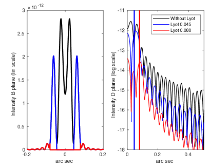
Figure 9: Left: residual image of the star (plane O’, in black) with two Lyot masks removing the first ring (in blue) or the second ring (in red). Middle: corresponding effects in the final plane D using a severe Lyot stop (diameter reduction 0.8). Only the largest mask allows notable rejection but at the expenses of image reconstruction in the vignetting zone. The vertical lines give the diameters of the Lyot masks. The figure on the right is a hybrid 2D representation that shows the two straylight rings and occulter Fresnel diffraction projected onto the sky.

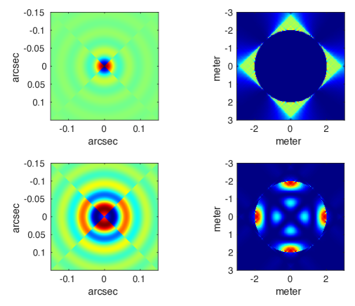
Figure 10: Illustration of the lack of efficiency of a 4-quadrant system with a Starshade. The top left figure corresponds to the Airy pattern (real part of the amplitude) given by a circular aperture with the $\pm 1$ transmission of the 4 quadrant mask. The top right figure is the corresponding intensity in plane C. A total rejection of the starlight in plane D can be obtained using a Lyot stop in plane C (see Fig.7 for planes denomination). Bottom figures are for the same planes with the external occulter. There is no more an Airy pattern in the plane B and the wave remains unfortunately inside the aperture image in plane C.

4 Benefit of adding an internal coronagraph

For the observation of the solar corona, a complementary Lyot coronagraph is used. Figure 7 gives the schematic diagram of a Lyot coronagraph coupled to an external occulter. The original Lyot coronagraph is slightly modified in order to set the mask (called the internal occulter) on the image of the external occulter. To simplify numerical calculations it is interesting to add a converging lens in plane A so as to reject the occulter to infinity and to compensate it with a diverging lens of the same negative power in C. The propagation of the wave is then done using three Fourier transforms, from A to O’, O’ to C, and C to D. Figure 8 shows that the coupling external occulter and Lyot coronagraph is very effective, and results in a stray light below $10^{-10}$, for perfect optics.

For the detection of exoplanets, projects are either with an external occulter alone or with an internal coronagraph alone. The schematic diagram of Fig.7 would still describe a system using a Lyot coronagraph after the starshade. The same calculation procedure can be made. In this case, given the very large distance where the external occulter is located, it will no longer be possible to differentiate experimentally plane O’ from plane B. We give in Fig.9 the effect of a Lyot coronagraph with a small mask of size the first ring, and with a large mask of size the second ring, using a very strong Lyot stop. The small mask will not affect the observation of exoplanets, but its effect on straylight is weak. The large mask is more effective in terms of straylight but it prevents the detection of exoplanets in the vignetting zone corresponding to the petals edges.

Finally, one might wonder whether a phase filter system would be more efficient than a Lyot coronagraph. Fig.10 illustrates that a 4 quadrant phase mask placed at the focus of a telescope [22] is not efficient either.

References

- [1] Lyot, B., “The study of the solar corona without an eclipse (with plate v),” Journal of the Royal Astronomical Society of Canada 27, 265 (1933).
- [2] Newkirk, Jr., G. and Bohlin, D., “Reduction of scattered light in the coronagraph,” Appl. Optics 2, 131 (Feb. 1963).
- [3] Newkirk, Jr., G. and Bohlin, J. D., “Coronascope II : observation of the white light corona from a stratospheric balloon,” in [Astronomical Observations from Space Vehicles ], Steinberg, J.-L., ed., IAU Symposium 23, 287 (1965).
- [4] Evans, J. W., “Photometer for measurement of sky brightness near the sun,” J. Opt. Soc. Am. 38, 1083 (Dec. 1948).
- [5] Koutchmy, S., “Space-borne coronagraphy,” Space science reviews 47(1), 95–143 (1988).
- [6] Tousey, R., “Observations of the white light corona by rocket,” Annales d’Astrophysique 28, 600 (Feb. 1965).
- [7] Purcell, J. and Koomen, M., “Coronagraph with improved scattered-light properties,” J. Opt. Soc. Am. 52, 596–597 (1962).
- [8] Brueckner, G., Howard, R., Koomen, M., Korendyke, C., Michels, D., Moses, J., Socker, D., Dere, K., Lamy, P., Llebaria, A., et al., “The large angle spectroscopic coronagraph (lasco) visible light coronal imaging and spectroscopy,” The SOHO mission , 357–402 (1995).
- [9] Bout, M., Lamy, P., Maucherat, A., Colin, C., and Llebaria, A., “Experimental study of external occulters for the large angle and spectrometric coronagraph 2: Lasco-c2,” Appl. Opt. 39, 3955–3962 (Aug 2000).
- [10] Boivin, L., “Reduction of diffraction errors in radiometry by means of toothed apertures,” Applied Optics 17(20), 3323–3328 (1978).
- [11] Rougeot, R. and Aime, C., “Theoretical performance of serrated external occulters for solar coronagraphy-application to aspiics,” Astronomy & Astrophysics 612, A80 (2018).
- [12] Aime, C., “Theoretical performance of solar coronagraphs using sharp-edged or apodized circular external occulters,” Astronomy & Astrophysics 558, A138 (2013).
- [13] Aime, C., “Fresnel diffraction of multiple disks on axis-application to coronagraphy,” Astronomy & Astrophysics 637, A16 (2020).
- [14] Cady, E., “Boundary diffraction wave integrals for diffraction modeling of external occulters,” Opt. Expr. 20(14), 15196–15208 (2012).
- [15] Cash, W., “Detection of earth-like planets around nearby stars using a petal-shaped occulter,” Nature 442(7098), 51 (2006).
- [16] Vanderbei, R. J., Cady, E., and Kasdin, N. J., “Optimal occulter design for finding extrasolar planets,” The Astrophysical Journal 665(1), 794 (2007).
- [17] Kasdin, N. J., Cady, E. J., Dumont, P. J., Lisman, P. D., Shaklan, S. B., Soummer, R., Spergel, D. N., and Vanderbei, R. J., “Occulter design for theia,” in [Techniques and Instrumentation for Detection of Exoplanets IV ], 7440, 30–37, SPIE (2009).
- [18] Flamary, R. and Aime, C., “Optimization of starshades: focal plane versus pupil plane,” Astronomy & Astrophysics 569, A28 (2014).
- [19] Marchal, C., “Concept of a space telescope able to see the planets and even the satellites around the nearest stars,” Acta Astronautica 12(3), 195–201 (1985).
- [20] Hildebrandt, S. R., Shaklan, S. B., Cady, E. J., and Turnbull, M. C., “Starshade imaging simulation toolkit for exoplanet reconnaissance,” Journal of Astronomical Telescopes, Instruments, and Systems 7(2), 021217 (2021).
- [21] Rougeot, R., Flamary, R., Galano, D., and Aime, C., “Performance of the hybrid externally occulted Lyot solar coronagraph. Application to ASPIICS,” Astronomy & Astrophysics 599, A2 (Mar. 2017).
- [22] Rouan, D., Riaud, P., Boccaletti, A., Clénet, Y., and Labeyrie, A., “The four-quadrant phase-mask coronagraph. i. principle,” Publications of the Astronomical Society of the Pacific 112(777), 1479 (2000).