Lattice QCD calculation of the subtraction function in forward Compton amplitude

Abstract

The subtraction function plays a pivotal role in calculations involving the forward Compton amplitude, which is crucial for predicting the Lamb shift in muonic atom, as well as the proton-neutron mass difference. In this work, we present a lattice QCD calculation of the subtraction function using two domain wall fermion gauge ensembles at the physical pion mass. We utilize a recently proposed subtraction point, demonstrating its advantage in mitigating statistical and systematic uncertainties by eliminating the need for ground-state subtraction. Our results reveal significant contributions from $N\pi$ intermediate states to the subtraction function. Incorporating these contributions, we compute the proton, neutron and nucleon isovector subtraction functions at photon momentum transfer $Q^{2}\in[0,2]$ GeV². For the proton subtraction function, we compare our lattice results with chiral perturbation theory prediction at low $Q^{2}$ and with the results from the perturbative operator-product expansion at high $Q^{2}$. Finally, using these subtraction functions as input, we determine their contribution to two-photon exchange effects in the Lamb shift and isovector nucleon electromagnetic self-energy.

I Introduction

The Lamb shift has been instrumental in advancing our understanding of quantum electrodynamics (QED) and the structure of the atom. It refers to a slight difference in energy levels within the hydrogen atom that was not predicted by the Dirac equation. Modern precision measurements of the Lamb shift have reached a point that they can probe the internal structure of the proton. A landmark example is the 2010 measurement of the Lamb shift in muonic hydrogen Pohl et al. (2010), which yielded an exceptionally accurate determination of the proton charge radius - an order of magnitude more precise than previous world averages like the CODATA-2010 value Mohr et al. (2012). Theoretical uncertainties in extracting the proton charge radius from the muonic hydrogen Lamb shift are mainly due to the two-photon exchange (TPE) contribution, where the non-perturbative hadronic part is linked to the forward Compton amplitude. This presents a promising target for lattice QCD, with the first such calculation recently published Fu et al. (2022). On the other hand, previous studies have largely relied on dispersive analyses using experimental data as input Pachucki (1999); Martynenko (2006); Carlson and Vanderhaeghen (2011); Gorchtein et al. (2013); Tomalak (2019), supplemented by effective field theories Nevado and Pineda (2008); Birse and McGovern (2012); Alarcon et al. (2014); Peset and Pineda (2015); Alarcón et al. (2020), non-relativistic QED Hill and Paz (2011), and the operator-product expansion (OPE) Hill and Paz (2017). Such analyses require a subtraction function to ensure the convergence of the dispersive integral at large momentum transfers, and large uncertainties in this subtraction function limit the precision of the TPE calculations. A similar challenge arises in the dispersive analysis of the isovector nucleon electromagnetic self-energy, where the largest uncertainty also stems from the subtraction function Walker-Loud et al. (2012); Thomas et al. (2015); Tomalak (2020); Gasser et al. (2021, 2020).

The study of the subtraction function dates back to 1950s. In a foundational paper Chew et al. (1957), Chew, Goldberger, Low, and Nambu developed dispersion relations for forward Compton scattering, introducing a subtraction constant (the subtraction function in modern terminology) to account for uncertainties at low momentum transfers. While much of the Compton amplitude can be derived from experimental data using principles like analyticity and unitarity, the subtraction function remains inaccessible from direct measurements, making it a persistent challenge in modern dispersive analyses. Current calculations of the subtraction function rely on models, leading to significant variation depending on the chosen approach. Efforts to constrain the subtraction function incorporate theoretical insights at both low Caswell and Lepage (1986); Pachucki (1996); Pineda (2003, 2005); Hill and Paz (2011); Carlson and Vanderhaeghen (2011); Hill et al. (2013); Biloshytskyi et al. (2024) and high momentum transfers Collins (1979); Hill and Paz (2017), but the intermediate region remains poorly understood. A recent proposal suggests that dilepton electroproduction could further constrain the subtraction function, offering hope that future precision experiments at electron facilities such as MAMI, MESA, and JLab might shed light on this key quantity Pauk et al. (2020). Theoretically, a precise ab initio calculation, such as from lattice QCD, would greatly enhance the accuracy of theoretical predictions. Here, we present our lattice QCD calculation of the subtraction function.

II Choice of subtraction point

In Euclidean space, the spin-averaged forward doubly-virtual Compton scattering tensor is expressed in

$$\mathcal{T}_{\mu\nu}(P,Q) = \frac{1}{8\pi M}\int\mathrm{d}^{4}x\,e^{iQ\cdot x}\langle N|\operatorname{T}[J_{\mu}(x)J_{\nu}(0)]|N\rangle$$ (1)

$$= K_{1}(P,Q)\mathcal{T}_{1}(\nu,Q^{2})+K_{2}(P,Q)\mathcal{T}_{2}(\nu,Q^{2}),$$

where

$$K_{1}(P,Q) = -\delta_{\mu\nu}+\frac{Q_{\mu}Q_{\nu}}{Q^{2}},$$

$$K_{2}(P,Q) = -\frac{1}{M^{2}}\left(P_{\mu}-\frac{P\cdot Q}{Q^{2}}Q_{\mu}\right)\left(P_{\nu}-\frac{P\cdot Q}{Q^{2}}Q_{\nu}\right),$$ (2)

and $\nu=P\cdot Q/M$, with $P=(iM,\mathbf{0})$ and $Q=(Q_{0},\mathbf{Q})$ representing the Euclidean nucleon and photon four-momenta, respectively. $M$ is the nucleon mass, $J_{\mu,\nu}$ are the electromagnetic quark currents and $\mathcal{T}_{1,2}(\nu,Q)$ are the Lorentz scalar functions. When needed, we use the superscripts $(\mathrm{p})$ and $(\mathrm{n})$ to distinguish between proton and neutron scalar functions. The isovector Lorentz scalar functions are defined as $\mathcal{T}_{1,2}^{(\mathrm{v})}=\mathcal{T}_{1,2}^{(\mathrm{p})}-\mathcal{T}_{1,2}^{(\mathrm{n})}$.

The TPE correction to the Lamb shift of a hydrogen-like atom is

$$\Delta E = -\frac{8m\alpha_{\mathrm{em}}^{2}}{\pi}\absolutevalue{\phi_{n}(0)}^{2}\int\mathrm{d}^{4}Q$$

$$\times \frac{(Q^{2}+2Q_{0}^{2})\mathcal{T}_{1}(iQ_{0},Q^{2})-(Q^{2}-Q_{0}^{2})\mathcal{T}_{2}(iQ_{0},Q^{2})}{Q^{4}(Q^{4}+4m^{2}Q_{0}^{2})},$$

with $\alpha_{\mathrm{em}}$ the fine structure constant, $m$ the lepton mass and $\absolutevalue{\phi_{n}(0)}^{2}$ the square of the $nS$-state wave function at the origin Carlson and Vanderhaeghen (2011). Similarly, $\mathcal{T}_{1,2}(\nu,Q)$ also appear in the nucleon electromagnetic self-energy, involving an integral of

$$\delta M^{\gamma}=\frac{\alpha_{\mathrm{em}}}{2\pi^{2}}\int_{R}\mathrm{d}^{4}Q\,\frac{-3Q^{2}\mathcal{T}_{1}(iQ_{0},Q^{2})+{\bf Q}^{2}\mathcal{T}_{2}(iQ_{0},Q^{2})}{Q^{4}}.$$ (4)

The subscript $R$ indicates that the integral has been renormalized, as discussed in Walker-Loud et al. (2012).

The scalar function $\mathcal{T}_{1,2}(\nu,Q^{2})$ encapsulate the complex structural information of the nucleon. They can be determined using dispersion relations Hagelstein et al. (2016)

$$\mathcal{T}_{1}(\nu,Q^{2}) - \mathcal{T}_{1}(\nu_{0},Q^{2})$$

$$= \int_{\nu_{\mathrm{el}}^{2}}^{\infty}\frac{\mathrm{d}{\nu^{\prime}}^{2}}{\pi}\frac{(\nu^{2}-\nu_{0}^{2})\operatorname{Im}\mathcal{T}_{1}(\nu^{\prime},Q^{2})}{({\nu^{\prime}}^{2}-\nu^{2})({\nu^{\prime}}^{2}-\nu_{0}^{2})},$$

$$\mathcal{T}_{2}(\nu,Q^{2}) = \int_{\nu_{\mathrm{el}}^{2}}^{\infty}\frac{\mathrm{d}{\nu^{\prime}}^{2}}{\pi}\frac{\operatorname{Im}\mathcal{T}_{2}(\nu^{\prime},Q^{2})}{{\nu^{\prime}}^{2}-\nu^{2}},$$ (5)

where $\nu_{\mathrm{el}}=Q^{2}/(2M)$. The imaginary parts of $\mathcal{T}_{1,2}(\nu,Q^{2})$ are related to the structure functions $F_{1,2}(\nu,Q^{2})$ as

$$\operatorname{Im}\mathcal{T}_{1}(\nu,Q^{2})=\frac{1}{4M}F_{1}(\nu,Q^{2}),$$

$$\operatorname{Im}\mathcal{T}_{2}(\nu,Q^{2})=\frac{1}{4\nu}F_{2}(\nu,Q^{2}).$$ (6)

$F_{1,2}(\nu,Q^{2})$ contain both elastic and inelastic contributions. The elastic part is described by the form factors

$$F_{1}^{\mathrm{el}}(\nu,Q^{2})=\frac{1}{2}G_{M}^{2}(Q^{2})\delta(1-x)$$

$$F_{2}^{\mathrm{el}}(\nu,Q^{2})=\frac{G_{E}^{2}(Q^{2})+\tau_{p}G_{M}^{2}(Q^{2})}{1+\tau_{p}}\delta(1-x),$$ (7)

where $\tau_{p}=Q^{2}/(4M^{2})$. The Bjorken variable is defined as $x\equiv Q^{2}/(2M\nu)$, so that $\delta(1-x)=\nu_{\mathrm{el}}\delta(\nu-\nu_{\mathrm{el}})$. $G_{E/M}(Q^{2})$ represent the electric and magnetic form factors. For the inelastic part, $F_{1,2}^{\mathrm{inel}}(\nu,Q^{2})$ are defined above the inelastic threshold, $\nu_{\mathrm{inel}}=m_{\pi}+(m_{\pi}^{2}+Q^{2})/(2M)$, and can be measured through electron or muon inelastic scattering.

In the dispersive framework, $\mathcal{T}_{1}(\nu_{0},Q^{2})$ in Eq. (II) represents the so-called subtraction function, with $\nu_{0}$ being the subtraction point, which is often chosen arbitrary. A common choice is $\nu_{0}=0$, as adopted by CSSM-QCDSF-UKQCD Collaboration in their exploratory lattice QCD study using Wilson fermions Hannaford-Gunn et al. (2022). Another subtraction point, $\nu_{0}=\frac{iQ}{2}$, has been proposed for the proton-neutron mass splitting Gasser et al. (2021, 2020). Recently, a new subtraction point at $\nu_{0}=iQ$ was suggested, which has the advantage of minimizing the inelastic contribution from the structure functions $F_{1,2}(\nu,Q^{2})$ to the muonic hydrogen Lamb shift Hagelstein and Pascalutsa (2021).

In this lattice QCD study, we find that choosing $\nu_{0}=iQ$ provides the most accurate estimate of the subtraction function. To illustrate this, we first introduced a generalized subtraction point, $\nu_{0}=i\xi Q$, where the four-momentum is specified as $Q_{0}=\xi Q$ and $|{\bf Q}|=\sqrt{1-\xi^{2}}Q$. Using this setup, we derive $\mathcal{T}_{1}(i\xi Q,Q^{2})$ from Eq. (1)

$$\mathcal{T}_{1}(i\xi Q,Q^{2}) = \frac{1}{2}\left[\frac{\xi^{2}}{1-\xi^{2}}\mathcal{T}_{00}-\sum_{i}\mathcal{T}_{ii}\right]$$ (8)

$$= \frac{1}{16\pi M}\int_{|t|<t_{0}}\mathrm{d}^{4}x\,e^{iQ\cdot x}$$

$$\hskip 28.45274pt\times\left[\frac{\xi^{2}}{1-\xi^{2}}H_{00}(x)-\sum_{i}H_{ii}(x)\right],$$

where $H_{\mu\nu}(x)=\langle N|T[J_{\mu}(x)J_{\nu}(0)]|N\rangle$ and $t_{0}$ represents the temporal truncation. According to the current conservation and Ward identity, the hadronic function $H_{\mu\nu}(x)$ satisfies Fu et al. (2022)

$$\int_{|t|<t_{0}}\mathrm{d}^{4}x\,H_{00}(x)=4Mt_{0}\,G_{E}^{2}(0),$$

$$\int_{|t|<t_{0}}\mathrm{d}^{4}x\,\sum_{i}H_{ii}(x)=6\,G_{E}^{2}(0),$$ (9)

where a sufficiently large $t_{0}$ ensures the nucleon ground-state dominance in $H_{00}(x)\Big{|}_{t=t_{0}}$. These relations were also numerically confirmed in our previous study Wang et al. (2024).

We focus on $\mathcal{T}_{1}(i\xi Q,Q^{2})$ at low $Q^{2}$. However, as $Q\to 0$, we encounter the divergence as $t_{0}$ increases

$$\mathcal{T}_{1}(i\xi Q,Q^{2})\Big{|}_{Q=0}=\frac{1}{8\pi M}\left[\frac{\xi^{2}}{1-\xi^{2}}2Mt_{0}-3\right]G_{E}^{2}(0).$$ (10)

The issue arises because the limit $Q\to 0$ is taken before $t_{0}\to\infty$. To resolve this, $t_{0}\to\infty$ must be taken first. Since lattice QCD data cannot access infinitely large time slices, we reconstruct the lattice data for $|t|>t_{0}$ using infinite-volume reconstruction method Feng and Jin (2019); Feng et al. (2022), or equivalently, replace the large-$t$ contribution with the ground-state contribution

$$\mathcal{T}_{1}(i\xi Q,Q^{2}) = \frac{1}{2}\left[\frac{\xi^{2}}{1-\xi^{2}}(\mathcal{T}_{00}-\mathcal{T}_{00}^{GS})-\sum_{i}(\mathcal{T}_{ii}-\mathcal{T}_{ii}^{GS})\right]$$ (11)

$$+\frac{1}{8\pi E}G_{E}^{2}(Q_{\mathrm{on}}^{2}),$$

where $Q_{\mathrm{on}}^{2}=2M(E-M)$ and $E=\sqrt{M^{2}+{\bf Q}^{2}}$. Here, $\mathcal{T}_{\mu\nu}^{GS}$ denotes the ground-state contribution to $\mathcal{T}_{\mu\nu}$. The derivation of Eq. (11) is provided in the Supplemental Material SM .

Although Eq. (11) allows for calculating the subtraction function at any subtraction point, the cancellation between $\mathcal{T}_{\mu\nu}$ and $\mathcal{T}_{\mu\nu}^{GS}$ introduces significant statistical and systematic uncertainties. However, a special case arises when $\xi=1$, or equivalently $\nu_{0}=iQ$, where the expression of $\mathcal{T}_{1}(iQ,Q^{2})$ simplifies to

$$\mathcal{T}_{1}(iQ,Q^{2}) = -\frac{1}{3}\sum_{i}T_{ii}$$ (12)

$$= -\frac{1}{24\pi M}\int\mathrm{d}t\,\cos(Qt)H(t).$$

Here hadronic function $H(t)$ is defined as $H(t)\equiv\int\mathrm{d}{\bf x}^{3}\,\sum_{i}H_{ii}(x)$. The derivation of Eq. (12) is provided in the Supplemental Material SM . Compared to the previous formalism (11), this approach no longer requires the subtraction of the ground-state contribution. From Eq. (II), we know that $\lim_{Q\to 0}\mathcal{T}_{1}(iQ,Q^{2})=-\frac{G_{E}^{2}(0)}{4\pi M}$. Thus, we define $T_{1}(iQ,Q^{2})$ as

$$T_{1}(iQ,Q^{2}) \equiv -\frac{4\pi\alpha_{\mathrm{em}}}{Q^{2}}\left[\mathcal{T}_{1}(iQ,Q^{2})-\lim_{Q\to 0}\mathcal{T}_{1}(iQ,Q^{2})\right]$$ (13)

$$= -\frac{\alpha_{\mathrm{em}}}{6M}\int\mathrm{d}t\,\frac{1-\cos(Qt)}{Q^{2}}H(t)$$

$$= \frac{\alpha_{\mathrm{em}}}{6M}\int\mathrm{d}t\,\frac{\cos(Qt)}{Q^{2}}H(t)+\alpha_{1}.$$ (14)

with $\alpha_{1}=-\frac{\alpha_{\mathrm{em}}G_{E}^{2}(0)}{MQ^{2}}$. Compared to $\mathcal{T}_{1}(iQ,Q^{2})$, $T_{1}(iQ,Q^{2})$ provides clearer insight into the low-$Q^{2}$ behavior. Additionally, direct insertion of $\mathcal{T}_{1}(iQ,Q^{2})$ into Eq. (II) leads to infrared divergence, whereas $T_{1}(iQ,Q^{2})$ is the commonly used function for calculating the Lamb shift Hill and Paz (2011, 2017); Biloshytskyi et al. (2024). Therefore, in this calculation, $T_{1}(iQ,Q^{2})$ is our primary target. Once $T_{1}(iQ,Q^{2})$ is determined, $\mathcal{T}_{1}(iQ,Q^{2})$ is also known.

III Numerical results

We used two $2+1$-flavor domain wall fermion ensembles from the RBC-UKQCD Collaboration Blum et al. (2016) at the physical pion mass, 24D and 32Df, with similar spatial volumes ($L=4.6$ fm) but different lattice spacings ($a^{-1}=1.023(2)$ GeV and $1.378(5)$ GeV). The hadronic functions $H_{\mu\nu}(x)$ from these ensemble, including both connected and disconnected diagrams, have been applied in previous studies of nucleon electric polarizabilities Wang et al. (2024) and electroweak box contributions to beta decays Ma et al. (2024).

As $Q\to 0$, $\alpha_{2}\equiv\lim_{Q\to 0}T_{1}(iQ,Q^{2})$ is known as

$$\alpha_{2} = -\frac{\alpha_{\mathrm{em}}}{12M}\int\mathrm{d}t\,t^{2}H(t)$$ (15)

$$= \alpha_{E}-\frac{\alpha_{\mathrm{em}}}{M}\left(\frac{G_{E}^{2}(0)+\kappa^{2}}{4M^{2}}+\frac{G_{E}(0)\langle r_{E}^{2}\rangle}{3}\right),$$

where $\alpha_{E}$ is the nucleon electric polarizability, $\kappa$ is the nucleon anomalous magnetic moment and $\langle r_{E}^{2}\rangle$ is the squared charge radius. In Ref. Wang et al. (2024), we confirmed that lattice QCD results for $\alpha_{E}$ are consistent with the PDG values Workman et al. (2022). To enhance the calculation, we can determine $T_{1}(iQ,Q^{2})$ by using experimental data for $\alpha_{E}$, $\kappa$ and $\langle r_{E}^{2}\rangle$ as input, and express $T_{1}(iQ,Q^{2})$ as

$$T_{1}(iQ,Q^{2})=-\frac{\alpha_{\mathrm{em}}}{6M}\int\mathrm{d}t\,\left[\frac{1-\cos(Qt)}{Q^{2}}-\frac{1}{2}t^{2}\right]H(t)+\alpha_{2}.$$ (16)

This expression is similar to those used for calculating hadronic vacuum polarization functions in muon $g-2$ studies Bernecker and Meyer (2011); Feng et al. (2013). When incorporating the experimental input for $\alpha_{2}$, the uncertainty is predominantly driven by $\alpha_{E}$.

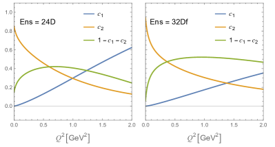
Figure 1: The parameters $c_{1}$, $c_{2}$ and the resulting $1-c_{1}-c_{2}$ as functions of $Q^{2}$ for the proton subtraction function, using both the 24D (left) and 32Df (left) ensembles.

Eq. (13) is the primary formula used to calculate $T_{1}(iQ,Q^{2})$, denoted as $T_{1}^{(0)}$. However, this method can suffer from large uncertainties at both the low- and high-$Q^{2}$. At low $Q^{2}$, Eq. (16) provides a more accurate estimate of $T_{1}(iQ,Q^{2})$ for the proton, as the uncertainty is mainly determined by $\alpha_{2}$, which is well-constrained by experimental data. At higher $Q^{2}$, Eq. (14) yields better results for $T_{1}(iQ,Q^{2})$ because the numerical integral is suppressed by the weight function $\cos(Qt)/Q^{2}$, and the remaining uncertainty from $\alpha_{1}$ is negligible. We define $T_{1}(iQ,Q^{2})$ from Eq. (14) as $T_{1}^{(1)}$ and from Eq. (16) as $T_{1}^{(2)}$. To take advantage of both approaches, we construct a new expression for $T_{1}(iQ,Q^{2})$ by introducing the parameters $c_{1}$ and $c_{2}$

$$T_{1}(iQ,Q^{2}) = (1-c_{1}-c_{2})T_{1}^{(0)}+c_{1}T_{1}^{(1)}+c_{2}T_{1}^{(2)}$$ (17)

$$= -\frac{\alpha_{\mathrm{em}}}{6M}\int\mathrm{d}t\,\left[\frac{1-c_{1}-\cos(Qt)}{Q^{2}}-\frac{c_{2}}{2}t^{2}\right]H(t)$$

$$+c_{1}\alpha_{1}+c_{2}\alpha_{2}.$$

To determine the optimal values for $c_{1}$ and $c_{2}$, we minimize the variance of the combined result $T_{1}(iQ,Q^{2})$. The values of $c_{1}$ and $c_{2}$ obtained through this minimization process. Fig. 1 shows $c_{1}$, $c_{2}$ and $1-c_{1}-c_{2}$ as functions of $Q^{2}$ for the case of the proton subtraction function. The corresponding results for the neutron and isovector subtraction functions are discussed in the Supplemental Material SM . We observe similar behavior in the 24D and 32Df ensembles. Note that it is not necessary to fix $c_{1,2}$ for all ensembles. In principle, $c_{1,2}$ can take arbitrary values. The different choices of $c_{1,2}$ may lead to varying statistical and systematic effects, but the methodology for determining $T_{1}(iQ,Q^{2})$ remains consistent. For the proton, the PDG value for the electric polarizability is $\alpha_{E}^{\mathrm{(p)}}=11.2(4)\times 10^{-4}$ fm³, with a few-percent precision, whereas uncertainties in the lattice results remain much larger. Consequently, at low $Q^{2}$, $c_{2}$ is significantly larger than both $c_{1}$ and $1-c_{1}-c_{2}$, indicating that $T_{1}(iQ,Q^{2})$ is primarily determined by $T_{1}^{(2)}$. As $Q^{2}$ increases, $c_{2}$ decreases while $c_{1}$ increases, causing $T_{1}^{(1)}$ to dominate. However, this pattern is not universal. In the isovector case, the disconnected diagrams in the lattice calculation cancel out, and the lattice results become more accurate as $Q\to 0$. Thus, the pure lattice results, $T_{1}^{(0)}$, dominate at low $Q^{2}$. Further details are available in the Supplemental Material SM .

In the realistic calculation of $T_{1}(iQ,Q^{2})$ using Eq. (17), the hadronic function $H(t)$ is computed from lattice QCD, which can be affected by various systematic effects. Among these, temporal truncation effects and finite-volume effects are most significant. To mitigate these systematic effects, we compute the matrix elements $\langle N|J_{i}(0)|N\pi\rangle$ for the four lowest $N\pi$ states in the center-of-mass frame, with nucleon momenta reaching up to $\sim 0.5$ GeV. A detailed discussion on controlling these systematic effects can be found in the Supplemental Material SM .

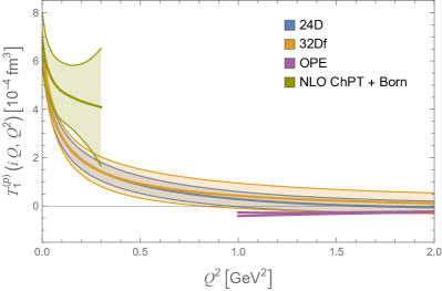
Figure 2: The lattice results of $T_{1}^{(\mathrm{p})}(iQ,Q^{2})$ as functions of $Q^{2}$. These results are compared with ChPT at low $Q^{2}$ Biloshytskyi et al. (2024) and with the perturbative OPE results at high $Q^{2}$ Hill and Paz (2017).

Fig. 2 shows the final results for $T_{1}^{(\mathrm{p})}(iQ,Q^{2})$, with the corresponding results for $T_{1}^{(\mathrm{n})}(iQ,Q^{2})$ and $T_{1}^{(\mathrm{v})}(iQ,Q^{2})$ provided in the Supplemental Material SM . The lattice results of $T_{1}^{(\mathrm{p})}(iQ,Q^{2})$ are compared with chiral perturbation theory (ChPT) predictions at low $Q^{2}$ Biloshytskyi et al. (2024), where the Born contribution

$$T_{1}^{B}(iQ,Q^{2}) = -\frac{\alpha_{\mathrm{em}}}{MQ^{2}}\Big{[}\frac{\tau_{p}G_{M}^{2}(Q^{2})}{1+\tau_{p}}+G_{E}^{2}(0)$$ (18)

$$-\Big{(}\frac{G_{E}(Q^{2})+\tau_{p}G_{M}(Q^{2})}{1+\tau_{p}}\Big{)}^{2}\Big{]}$$

has been subtracted. For comparison, we add back the Born contribution using the form factors from Ref. Borah et al. (2020). The main uncertainty in the ChPT results arises from the non-Born part. At large $Q^{2}$, the lattice results are compared with one-loop perturbative OPE predications Hill and Paz (2017). The results show similar behavior to both ChPT at low $Q^{2}$ and OPE at high $Q^{2}$, with smaller uncertainties at low $Q^{2}$ and providing new insights in the intermediate region, which is not well-covered by either method.

IV Applications of subtraction function

Although the TPE contribution to the Lamb shift in Eq. (II) is infrared divergent, this divergence can be eliminated by subtracting the contributions from a pointlike term and the third Zemach moment Carlson and Vanderhaeghen (2011). For the subtraction-function contribution, the infrared divergence can be simply removed by performing the subtraction of $\mathcal{T}_{1}(iQ,Q^{2})-\lim_{Q\to 0}\mathcal{T}_{1}(iQ,Q^{2})$. The contribution to the Lamb shift is then given by

$$\Delta E_{\mathrm{sub}}\Big{|}_{\Lambda^{2}} = \frac{8m\alpha_{\mathrm{em}}^{2}}{\pi}\absolutevalue{\phi_{n}(0)}^{2}$$

$$\times\int_{Q^{2}<\Lambda^{2}}\frac{\mathrm{d}^{4}Q}{Q^{2}}\frac{Q^{2}+2Q_{0}^{2}}{Q^{4}+4m^{2}Q_{0}^{2}}T_{1}(iQ,Q^{2})$$

$$= \frac{4\pi\alpha_{\mathrm{em}}^{2}}{m}\absolutevalue{\phi_{n}(0)}^{2}\int_{0}^{\Lambda^{2}}\mathrm{d}Q^{2}\,\frac{\gamma_{1}(\tau)}{\sqrt{\tau}}T_{1}(iQ,Q^{2})$$

where $\gamma_{1}(\tau)=(1-2\tau)\left[(1+\tau)^{\frac{1}{2}}-\tau^{\frac{1}{2}}\right]+\tau^{\frac{1}{2}}$ and $\tau=Q^{2}/(4m^{2})$.

By substituting the lattice results of the subtraction function $T_{1}(iQ,Q^{2})$ into the integral and applying momentum cutoffs of $\Lambda^{2}=1$ GeV² and 2 GeV², we obtain for the following subtraction-function contributions to the muonic hydrogen Lamb shift

$$\Delta E_{\mathrm{sub}}^{(\mathrm{p})}\Big{|}_{\Lambda^{2}=1\leavevmode\nobreak\ \mathrm{GeV}^{2}} = \begin{cases}6.94(42)(54)\mbox{ $\mu$eV}&\mbox{for 24D}\\ 7.15(70)(54)\mbox{ $\mu$eV}&\mbox{for 32Df}\end{cases},$$

$$\Delta E_{\mathrm{sub}}^{(\mathrm{p})}\Big{|}_{\Lambda^{2}=2\leavevmode\nobreak\ \mathrm{GeV}^{2}} = \begin{cases}6.97(47)(56)\mbox{ $\mu$eV}&\mbox{for 24D}\\ 7.22(81)(57)\mbox{ $\mu$eV}&\mbox{for 32Df}\end{cases}.$$ (20)

The first uncertainty is the lattice statistical error, and the second is from experimental input. The results for 24D and 32Df are in very good agreement, and the results at $\Lambda^{2}=1$ GeV² and 2 GeV² are nearly the same, with only sub-percent changes. This is expected, as the integral is ultraviolet finite and thus not sensitive to high-momentum regions. The contribution above $\Lambda^{2}$ can be estimated using perturbative OPE, which is found to be negligible.

For neutron subtraction function, its contribution to the muonic-atom Lamb shift is

$$\Delta E_{\mathrm{sub}}^{(\mathrm{n})}\Big{|}_{\Lambda^{2}=1\leavevmode\nobreak\ \mathrm{GeV}^{2}} = \begin{cases}10.49(90)(77)\mbox{ $\mu$eV}&\mbox{for 24D}\\ 12.5(1.0)(1.0)\mbox{ $\mu$eV}&\mbox{for 32Df}\end{cases},$$

$$\Delta E_{\mathrm{sub}}^{(\mathrm{n})}\Big{|}_{\Lambda^{2}=2\leavevmode\nobreak\ \mathrm{GeV}^{2}} = \begin{cases}10.60(96)(80)\mbox{ $\mu$eV}&\mbox{for 24D}\\ 12.7(1.1)(1.1)\mbox{ $\mu$eV}&\mbox{for 32Df}\end{cases}.$$ (21)

Here, the wave function $\absolutevalue{\phi_{n}(0)}^{2}$ is still taken from muonic hydrogen Tomalak (2019). When applying the neutron subtraction function to muonic atoms like muonic deuterium and muonic helium, $\absolutevalue{\phi_{n}(0)}^{2}$ needs to be rescaled Krauth et al. (2016); Diepold et al. (2018); Franke et al. (2017). Again, the results at $\Lambda^{2}=1$ GeV² and 2 GeV² are consistent and the 24D and 32Df results have a slight deviation of $\sim 1.5$ $\sigma$.

The subtraction-function contribution to the isovector nucleon self-energy can be computed as

$$\delta M_{\mathrm{sub}}^{\gamma,(\mathrm{v})}\Big{|}_{\Lambda^{2}} = -\frac{3\alpha_{\mathrm{em}}}{2}\int_{0}^{\Lambda^{2}}\mathrm{d}Q^{2}\,\mathcal{T}_{1}^{(\mathrm{v})}(iQ,Q^{2})$$ (22)

$$= \frac{3}{8\pi}\int_{0}^{\Lambda^{2}}\mathrm{d}Q^{2}\left[Q^{2}T_{1}^{(\mathrm{v})}(iQ,Q^{2})+\frac{\alpha_{\mathrm{em}}}{M}\right].$$

Using the isovector subtraction function as input, we obtain the nucleon self-energy in MeV

$$\delta M_{\mathrm{sub}}^{\gamma,(\mathrm{v})}\Big{|}_{\Lambda^{2}=1\leavevmode\nobreak\ \mathrm{GeV}^{2}} = \begin{cases}-0.672(36)(04)+0.928&\mbox{for 24D}\\ -0.648(46)(09)+0.928&\mbox{for 32Df}\end{cases},$$

$$\delta M_{\mathrm{sub}}^{\gamma,(\mathrm{v})}\Big{|}_{\Lambda^{2}=2\leavevmode\nobreak\ \mathrm{GeV}^{2}} = \begin{cases}-1.643(54)(09)+1.857&\mbox{for 24D}\\ -1.611(77)(17)+1.857&\mbox{for 32Df}\end{cases}.$$

The two terms arise from $Q^{2}T_{1}^{(\mathrm{v})}(iQ,Q^{2})$ and $\alpha_{\mathrm{em}}/M$, respectively. The nucleon self-energy computed here is only meaningful when a momentum cutoff is applied, as the integral is ultraviolet divergent. For each $\Lambda^{2}$, the 24D and 32Df results show good agreement. Currently, the largest uncertainty, 0.08 MeV, arises from the 32Df case with $\Lambda^{2}=2\leavevmode\nobreak\ \mathrm{GeV}^{2}$. This uncertainty is already much smaller than those reported in previous dispersive analyses Walker-Loud et al. (2012); Thomas et al. (2015); Tomalak (2020); Gasser et al. (2021, 2020), where reducing model dependence is essential for achieving a robust error estimate.

V Conclusion and discussion

In this work, we performed a detailed lattice QCD calculation of the proton, neutron, and isovector subtraction functions. The use of a new subtraction point allowed us to reduce statistical and systematic uncertainties, particularly by avoiding the need for ground-state subtraction. The use of two gauge ensembles at the physical pion mass allowed us to obtain results directly at the physical point, but also introduced significant temporal truncation and finite-volume effects. By calculating the $N\pi$-state contributions with center-of-mass momentum up to $\sim$0.5 GeV, we were able to control both of these systematic effects. The final lattice results provide a valuable comparison with previous theoretical predictions at low and high $Q^{2}$, while also offering novel insights in the intermediate momentum region.

We applied these subtraction functions to compute the TPE contribution to the Lamb shift in muonic atom, as well as the isovector nucleon self-energy. In all cases, uncertainties were significantly reduced due to improved knowledge of the structure function in the intermediate momentum region and smaller uncertainties at low momentum.

Given the challenges associated with the physical pion mass, performing the calculation at heavier pion masses, as done by the CSSM-QCDSF-UKQCD Collaboration, followed by a chiral extrapolation, is a promising alternative approach. It is worth noting that even at unphysical pion masses, such as 300 MeV, controlling temporal truncation and finite-volume effects remains crucial.

VI Supplemental Material

VI.1 Derivation of Eq. (11) and (12)

If $Q$ approaches zero first, the subtraction function $T(i\xi Q,Q^{2})$ defined in Eq. (8) encounters a linear divergence as the temporal truncation parameter $t_{0}$ increases. To resolve this issue, we modify the expression as given in Eq. (11). Below, we provide the derivations that leads to Eq. (11).

The term $\mathcal{T}^{GS}_{\mu\nu}$ accounts for the ground-state contribution to $\mathcal{T}_{\mu\nu}$. Before taking the limit $Q\to 0$, we first compute $\mathcal{T}^{GS}_{00}$ and $\sum_{i}\mathcal{T}^{GS}_{ii}$ for non-zeo $Q$, using

$$\mathcal{T}^{GS}_{\mu\nu} = \frac{1}{8\pi M}\int\mathrm{d}^{4}x\,e^{iQ\cdot x}H_{\mu\nu}^{GS}(x)$$ (S 1)

$$= \frac{1}{4\pi E}\frac{Q_{\mathrm{on}}^{2}}{Q_{\mathrm{on}}^{2}+4M^{2}Q_{0}^{2}}\mathcal{M}_{\mu\nu}({\bf Q}),$$

where $Q=(Q_{0},{\bf Q})$, $E=\sqrt{M^{2}+{\bf Q}^{2}}$, $H_{\mu\nu}^{GS}(x)$ is the ground-state contribution to $H_{\mu\nu}(x)$ and

$$\mathcal{M}_{\mu\nu}({\bf Q})\equiv\langle N(\mathbf{0})|J_{\mu}(0)|N(\mathbf{Q})\rangle\langle N(\mathbf{Q})|J_{\nu}(0)|N(\mathbf{0})\rangle.$$ (S 2)

The squared momentum $Q_{\mathrm{on}}^{2}$ results from the momentum transfer between two on-shell states and is proportional to ${\bf Q}^{2}$

$$Q_{\mathrm{on}}^{2}=(iE-iM)^{2}+{\bf Q}^{2}=2M(E-M)=\frac{2M}{E+M}{\bf Q}^{2}.$$ (S 3)

By expressing $\langle N(\mathbf{0})|J_{\mu}(0)|N(\mathbf{Q})\rangle$ in terms of form factors, we obtain

$$T_{00}^{GS} = \frac{1}{4\pi E}\frac{4M^{2}{\bf Q}^{2}}{Q_{\mathrm{on}}^{4}+4M^{2}Q_{0}^{2}}G_{E}^{2}(Q_{\mathrm{on}}^{2}),$$

$$\sum_{i}T_{ii}^{GS} = -\frac{1}{4\pi E}\frac{Q_{\mathrm{on}}^{4}}{Q_{\mathrm{on}}^{4}+4M^{2}Q_{0}^{2}}G_{E}^{2}(Q_{\mathrm{on}}^{2}),$$ (S 4)

and their combination

$$\frac{1}{2}\left[\frac{\xi^{2}}{1-\xi^{2}}T_{00}^{GS}-\sum_{i}T_{ii}^{GS}\right]=\frac{1}{8\pi E}G_{E}^{2}(Q_{\mathrm{on}}^{2}).$$ (S 5)

By combining Eq. (S 5) with Eq. (8), we immediately arrive at Eq. (11). Since the combination of $T_{00}-T_{00}^{GS}$ and $T_{ii}-T_{ii}^{GS}$ completely removes the long-distance contribution, the divergence issue is resolved. Therefore, Eq. (11) remains valid even taking the limit $Q\to 0$ before $t_{0}\to\infty$.

The next task is to derive Eq. (12). Starting from Eq. (1), we have

$$\delta_{\mu\nu}\mathcal{T}_{\mu\nu}=\mathcal{T}_{00}+\sum_{i}\mathcal{T}_{ii}=-3\mathcal{T}_{1}+(1-\xi^{2})\mathcal{T}_{2}$$

$$-\frac{P_{\mu}P_{\nu}}{M^{2}}\mathcal{T}_{\mu\nu}=\mathcal{T}_{00}=-(1-\xi^{2})\mathcal{T}_{1}+(1-\xi^{2})^{2}\mathcal{T}_{2}$$ (S 6)

From the second equation, we otain

$$\mathcal{T}_{1}=-\frac{1}{1-\xi^{2}}\mathcal{T}_{00}+(1-\xi^{2})\mathcal{T}_{2}.$$ (S 7)

Substituting this into the first equation and imposing the condition $(1-\xi^{2})\mathcal{T}_{2}\Big{|}_{\xi=1}=0$, we obtain

$$\sum_{i}T_{ii}\Big{|}_{\xi=1}=\frac{2+\xi^{2}}{1-\xi^{2}}\mathcal{T}_{00}\Big{|}_{\xi=1}=3\frac{\mathcal{T}_{00}}{1-\xi^{2}}\Big{|}_{\xi=1}.$$ (S 8)

At $\xi=1$, replacing $\frac{\xi^{2}}{1-\xi^{2}}\mathcal{T}_{00}\Big{|}_{\xi=1}$ in Eq. (8) with $\frac{1}{3}\sum_{i}T_{ii}\Big{|}_{\xi=1}$, we arrive at Eq. (12).

VI.2 Systematic effects

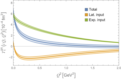
Figure S 1: A comparison between the contributions to $T_{1}^{(\mathrm{p})}(iQ,Q^{2})$ from lattice QCD input and experimental input, using the 24D proton subtraction function as an example.

In Eq. (17), once the parameters $c_{1}$ and $c_{2}$ are determined, the integral part

$$T_{1}^{\mathrm{lat}}(iQ,Q^{2})=-\frac{\alpha_{\mathrm{em}}}{6M}\int\mathrm{d}t\,\omega(Q^{2},t)H(t)$$ (S 9)

with the weight function

$$\omega(Q^{2},t)=\left[\frac{1-c_{1}-\cos(Qt)}{Q^{2}}-\frac{c_{2}}{2}t^{2}\right]$$ (S 10)

is influenced by the lattice input through $H(t)$, while the term of $c_{1}\alpha_{1}+c_{2}\alpha_{2}$ is informed by experimental data. In Fig. S 1, using the 24D proton subtraction function as an example, we distinguish these two contributions. Across nearly the entire region of $Q^{2}\in[0,2]$ GeV², the lattice QCD input plays a significant role in determining $T_{1}(iQ,Q^{2})$.

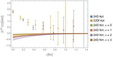
Figure S 2: The hadronic function $H^{(\mathrm{p})}(t)$ from both the 24D and 32Df ensembles as a function of $t$. These results are compared with the contributions from the four lowest $N\pi$ states, which are calculated using 24D ensemble.

In calculating $T_{1}^{\mathrm{lat}}(iQ,Q^{2})$, the lattice data for $H(t)$ become increasingly noisy as the time separation $t$ between the two currents grows, due to the signal-to-noise problem. To address this, a temporal truncation $t_{0}$ is introduced for the integral. As shown in Fig. S 2, clear signals are observed at small $t$, but quickly drown in noise. The data converge to $0$ around $0.75$ fm, so we set $t_{0}$ accordingly. However, this truncation introduces significant systematic effects caused by $N\pi$ intermediate states, which we will correct, as discussed below.

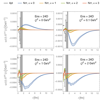
Figure S 3: The product of the weight function $\omega(Q^{2},t)$ and the hadronic function $H^{\mathrm{(p)}}(t)$ as a function of $t$ for $Q^{2}=0$ GeV², 0.1 GeV², 1 GeV² and 2 GeV². These results are compared with the contributions from the four lowest $N\pi$ states, using the 24D ensemble as an example.

At large time separation, $H(t)$ is dominated by the low-lying $N\pi$ intermediate states

$$H^{N\pi,n}(t) = \sum_{i}\langle N|J_{i}|N\pi,n\rangle\langle N\pi,n|J_{i}|N\rangle e^{-(E_{N\pi,n}-M)|t|}$$ (S 11)

$$= A_{n}e^{-\Delta E_{n}|t|},$$

where $|N\pi,n\rangle$ (with $n=0,1,2,3,\cdots$) represents the discrete energy eigenstates, ordered from lowest to highest, and $E_{N\pi,n}$ denotes their corresponding energies. Although $H^{N\pi,n}(t)$ are significantly smaller than the total $H(t)$, which is extracted from four-point correlation functions (as shown in Fig. S 2), they are amplified by the weight function $\omega(Q^{2},t)$. In Fig. S 3, we demonstrate that with $t_{0}=0.75$ fm, the integral is far from converged, as the integrand associated with the lowest $N\pi$ state peaks at $t_{\mathrm{peak}}=2$-4 fm for $Q^{2}=0$ GeV², 0.1 GeV², 1 GeV² and 2 GeV². At $Q^{2}=1$-2 GeV², the oscillatory behavior of $\omega(Q^{2},t)H(t)$ arises from the $\cos(Qt)$ factor in $\omega(Q^{2},t)$. In the previous study Wang et al. (2024), we calculated $H^{N\pi,n}(t)$ for the four lowest states, which mitigate the temporal truncation issue. However, direct summation over the discrete $N\pi$ states still suffers from significant finite-volume effects at $L\approx 4.6$ fm. To address both temporal truncation and finite-volume effects simultaneously, we replace the discrete finite-volume $N\pi$-state summation that includes temporal truncation at $t_{0}$

$$T_{1}^{N\pi}(t_{0},Q^{2},L)=-\frac{\alpha_{\mathrm{em}}}{6M}\int_{|t|<t_{0}}\mathrm{d}t\,\omega(Q^{2},t)\sum_{n\leq 3}A_{n}e^{-\Delta E_{n}|t|}$$ (S 12)

with the infinite-volume $N\pi$-state integral, which does not involve temporal truncation

$$T_{1}^{N\pi}(Q^{2},\infty) = -\frac{\alpha_{\mathrm{em}}}{6M}\int\mathrm{d}t\,\omega(Q^{2},t)$$ (S 13)

$$\times\int_{|{\bf p}|<\Lambda}\frac{\mathrm{d}^{3}{\bf p}}{(2\pi)^{3}}\,A_{\infty}({\bf p}^{2})e^{-\Delta E|t|}$$

where $\Delta E=\sqrt{M^{2}+{\bf p}^{2}}+\sqrt{M_{\pi}^{2}+{\bf p}^{2}}-M$, with ${\bf p}$ being the nucleon’s momentum in the $N\pi$ center-of-mass frame. The quantity $A_{\infty}$ is converted from $A_{n}$ by multiplying a conversion factor $\frac{L^{3}}{\nu_{n}}$ (with $\nu_{n}=1,6,12,8$ for $n=0,1,2,3$). This conversion factor is equivalent to the Lellouch-Lüscher factor when $N\pi$-rescattering effects are neglected. The ${\bf p}^{2}$-dependence of $A_{\infty}({\bf p}^{2})$ has been determined in our previous study Wang et al. (2024). In relation to the discrete states $n=0,1,2,3$, we introduce the momentum cutoff $\Lambda_{0}$ as

$$\Lambda_{0}=\left(\frac{2\pi}{L}\right)\left(\left(\sum_{n=0}^{3}\nu_{n}\right)/\left(\frac{4}{3}\pi\right)\right)^{\frac{1}{3}}\approx 0.5\mbox{ GeV}.$$ (S 14)

In Fig. S 4, we compare $T_{1}^{N\pi}(Q^{2},\infty)$ for the regions $|{\bf p}|<\Lambda_{0}$ and $\Lambda_{0}<|{\bf p}|<\Lambda_{1}$, where $\Lambda_{1}=1$ GeV. We assume that ${\bf p}^{2}$-dependence of $A_{\infty}({\bf p}^{2})$, determined for $|{\bf p}|<\Lambda_{0}$, remains valid for $\Lambda_{0}<|{\bf p}|<\Lambda_{1}$. For $|{\bf p}|>\Lambda_{1}$, however, the ${\bf p}^{2}$-dependence of $A_{\infty}({\bf p}^{2})$ is likely no longer applicable. Nevertheless, the much smaller contribution from the region $\Lambda_{0}<|{\bf p}|<\Lambda_{1}$ compared to $|{\bf p}|<\Lambda_{0}$ suggests that the residual temporal truncation and finite-volume effects associated with the higher states are no longer significant.

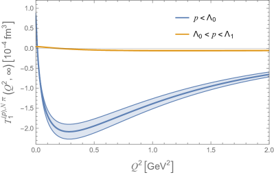
Figure S 4: Comparison of $T_{1}^{N\pi}(Q^{2},\infty)$ for momentum regions $|{\bf p}|<\Lambda_{0}$ and $\Lambda_{0}<|{\bf p}|<\Lambda_{1}$, with $\Lambda_{0}$ defined in Eq. (S 14) and $\Lambda_{1}=1$ GeV. The contribution from the higher momentum region $\Lambda_{0}<|{\bf p}|<\Lambda_{1}$ is substantially smaller than that from the lower momentum region $|{\bf p}|<\Lambda_{0}$, suggesting that residual temporal truncation and finite-volume effects associated with higher states are no longer significant.

VI.3 Numerical results for neutron and isovector subtraction function

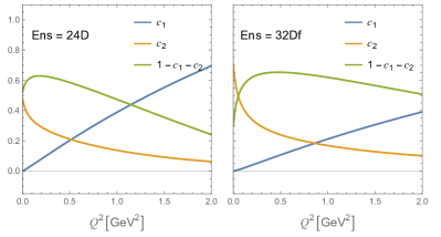
Figure S 5: The parameters $c_{1}$, $c_{2}$ and $1-c_{1}-c_{2}$ as functions of $Q^{2}$ for the neutron subtraction function, using both the 24D (left) and 32Df (right) ensembles.

For the neutron subtraction function, the parameters $c_{1}$, $c_{2}$ and $1-c_{1}-c_{2}$ are shown in Fig. S 5. Since the experimental measurements of $\alpha_{E}^{(\mathrm{n})}$ are not as precise as those for $\alpha_{E}^{(\mathrm{p})}$, the $\alpha_{2}$ term does not impose a strong constraint at low $Q^{2}$. We observe that as $Q\to 0$, the value of $c_{2}$ deviates from 1 more significantly compared to the proton case. Using $c_{1}$ and $c_{2}$ as inputs, the final results for $T_{1}^{(\mathrm{n})}(iQ,Q^{2})$ are shown in Fig. S 6.

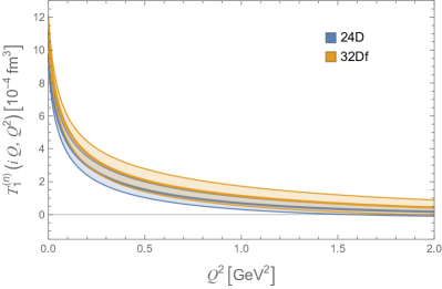
Figure S 6: The lattice results of $T_{1}^{(\mathrm{n})}(iQ,Q^{2})$ as functions of $Q^{2}$.

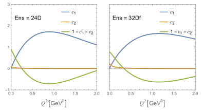
Figure S 7: The parameters $c_{1}$, $c_{2}$ and $1-c_{1}-c_{2}$ as functions of $Q^{2}$ for the isovector subtraction function, using both the 24D (left) and 32Df (left) ensembles.

For the isovector subtraction function, the parameters $c_{1}$, $c_{2}$ and $1-c_{1}-c_{2}$ are shown in Fig. S 7. We assume that the experimental measurements of $\alpha_{E}^{(\mathrm{p})}$ and $\alpha_{E}^{(\mathrm{n})}$ are uncorrelated, so the combined error is taken as the square root of the sum of squares. In contrast, for the lattice QCD input, the disconnected diagram cancels in the isovector case, causing the lattice results to dominate the variance minimization process. Consequently, $1-c_{1}-c_{2}$ is very close to 1. The final results for $T_{1}^{(\mathrm{v})}(iQ,Q^{2})$ are presented in Fig. S 8. These results align with the combination $T_{1}^{(\mathrm{p})}(iQ,Q^{2})-T_{1}^{(\mathrm{n})}(iQ,Q^{2})$, with only slight differences. This is because we determine $T_{1}^{(\mathrm{v})}(iQ,Q^{2})$ using the $c_{1,2}$ values from the variance minimization process, rather than relying on the inputs of $T_{1}^{(\mathrm{p})}(iQ,Q^{2})$ and $T_{1}^{(\mathrm{n})}(iQ,Q^{2})$.

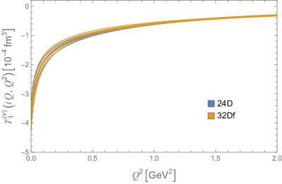
Figure S 8: The lattice results of $T_{1}^{(\mathrm{v})}(iQ,Q^{2})$ as functions of $Q^{2}$.