Predict-and-Optimize Robust Unit Commitment with Statistical Guarantees via Weight Combination

Abstract

The growing uncertainty from renewable power and electricity demand brings significant challenges to unit commitment (UC). While various advanced forecasting and optimization methods have been developed to predict better and address this uncertainty, most previous studies treat forecasting and optimization as separate tasks. This separation can lead to suboptimal results due to misalignment between the objectives of the two tasks. To overcome this challenge, we propose a robust UC framework that integrates the forecasting and optimization processes while ensuring statistical guarantees. In the forecasting stage, we combine multiple predictions derived from diverse data sources and methodologies for an improved prediction, aiming to optimize the UC performance. In the optimization stage, the combined prediction is used to construct an uncertainty set with statistical guarantees, based on which the robust UC model is formulated. The optimal robust UC solution provides feedback to refine the forecasting process, forming a closed loop. To solve the proposed integrated forecasting-optimization framework efficiently and effectively, we develop a neural network-based surrogate model for acceleration and introduce a reshaping method for the uncertainty set based on the optimization result to reduce conservativeness. Case studies on modified IEEE 30-bus and 118-bus systems demonstrate the advantages of the proposed approach.

Nomenclature

-A Abbreviation

C&CG

Column-and-constraint generation.

DRO

Distributionally robust optimization.

i.i.d.

Independent and identically distributed.

MILP

Mixed-integer linear programming.

RO

Robust optimization.

SP

Stochastic programming.

UC

Unit commitment.

-B Indices and Sets

$i\in\mathcal{I}$

Set of buses.

$m\in\mathcal{M}$

Set of prediction methods.

$x\in\mathcal{X}$

Feasible set of the pre-dispatch variable.

$u\in\mathcal{U}$

Uncertainty set.

$y\in\mathcal{Y}(x,u)$

Feasible set of the re-dispatch variable.

$g\in\mathcal{G}$

Set of generators.

$t\in\mathcal{T}$

Set of periods in unit commitment.

$l\in\mathcal{L}$

Set of transmission lines.

-C Parameters

$T$

The number of periods in a day.

$\varepsilon,\delta$

Probability tolerance parameters.

$N,N^{\prime}$

The number of data in the training/validation dataset.

$\hat{u}_{it}$

Prediction of load $i$ in period $t$.

$o_{g}^{+},o_{g}^{-}$

Startup/shutdown costs of generator $g$.

$\rho_{g}$

Generation cost coefficient of generator $g$.

$\gamma_{g}^{+},\gamma_{g}^{-}$

Upward/downward reserve cost coefficient of generator $g$.

$S_{l}$

Capacity of line $l$.

$\pi_{gl},\pi_{il}$

Power transfer distribution factor from generator $g$/bus $i$ to line $l$.

$T_{g}^{+},T_{g}^{-}$

Minimum up/down time of generator $g$.

$R_{g}^{+},R_{g}^{-}$

Maximum upward/downward reserve of generator $g$.

$\underline{P}_{g},\overline{P}_{g}$

Minimum/maximum output of generator $g$.

$K_{g}^{+},K_{g}^{-}$

Maximum upward/downward ramp of generator $g$ in a period.

$K_{g}^{U},K_{g}^{D}$

Maximum output increase/decrease when generator $g$ startups/shutdowns in a period.

$\rho_{g}^{+},\rho_{g}^{-}$

Upward/downward output adjustment cost coefficient of generator $g$.

$\underline{U},\overline{U}$

Lower/upper bounds of uncertain load.

$\underline{E},\overline{E}$

Lower/upper bounds of load forecast error.

-D Variables

$u_{it}$

Uncertain load at bus $i$ in period $t$.

$w$

Weight vector of predictions.

$\theta_{gt},\theta_{gt}^{+},\theta_{gt}^{-}$

Indicator variable for the on/startup/shutdown state of generator $g$ in period $t$.

$p_{gt}$

Day-ahead scheduled output of generator $g$ in period $t$.

$r_{gt}^{+},r_{gt}^{-}$

Upward/downward reserve of generator $g$ in period $t$.

$p_{gt}^{+},p_{gt}^{-}$

Upward/downward output adjustment of generator $g$ in period $t$.

I Introduction

The ongoing transition towards greener power systems has significantly increased the deployment of renewable power generators, leading to higher volatility in power sources. This uncertainty, together with the randomness of electric loads, presents great challenges for power system operations. Unit commitment (UC) is one of such power system operation problems that require particular attention.

If given the probability distribution of uncertainty, stochastic programming (SP) can be applied to UC problems to determine the optimal strategy [1]. However, an accurate probability distribution is difficult to obtain in reality and the inaccuracy of the distribution may jeopardize the feasibility and optimality of SP solutions. Robust optimization (RO) handles this problem by focusing on the worst-case scenario in a pre-defined uncertainty set. Fruitful research has been done in this area: A multi-stage robust UC model was proposed and solved by robust dual dynamic programming in [2]. Polyhedra were used to replace rectangular uncertainty sets to model the uncertainty correlations in [3]. However, RO can be overly conservative when the uncertainty set contains all the possible uncertainty realizations, because extreme scenarios rarely happen but can cause a steep cost increase. The method in [4] estimated quantiles from historical data to establish rectangular uncertainty sets, in which extreme scenarios were excluded. In [5], uncertainty budgets were used to restrict the uncertainty set. A decision-dependent uncertainty set was constructed in [6] to consider the impact of pricing on demand. However, estimated quantiles and uncertainty budgets may also be inaccurate, and the resulting uncertainty set lacks a statistical guarantee. This makes the obtained robust UC strategy less reliable and trustworthy.

Distributionally robust optimization (DRO) is another way to deal with uncertainty, which considers the worst-case probability distribution in a pre-defined ambiguity set. Two-stage distributionally robust UC methods were developed in [7] and [8] using Wasserstein metric ambiguity sets, while unimodality skewness of wind power was utilized in [9]. The copula theory was combined with DRO in [10] to better capture the dependence between uncertainty. Although data-driven DRO can have a statistical guarantee [7], the theoretical number of required data depends on the dimension of uncertainty, usually much larger than what is practically available. As a result, it is hard to adjust the size of the ambiguity set to obtain a satisfactory statistical guarantee.

Recently, a data-driven uncertainty set construction framework was proposed in [11] with a dimension-free statistical guarantee. Even for multidimensional uncertainty, it can provide a satisfactory statistical guarantee based on a moderate amount of data, enabling the decision-maker to effectively control the conservative degree and easily strike a balance between optimality and robustness. This method was applied to economic dispatch [12], scheduling of thermostatically controlled loads [13], and UC [14]. However, the static RO models in [12, 13, 14] cannot account for the re-dispatch stage, resulting in overly conservative day-ahead strategies. Therefore, a two-stage adjustable RO method with statistical guarantees is needed for the robust UC problem.

In addition, the quality of the uncertainty set relies heavily on the precision of the uncertainty forecasts. The predictions of different forecasting methods can be combined by a weight parameter to achieve a better performance than the individual methods [15]. Following this idea, an ensemble deep learning method was proposed in [16] for probabilistic wind power forecasting, where the weight parameter was determined according to a quantile loss index. The extreme prediction risk was modeled by the conditional value-at-risk in [17] to optimize the ensemble weight of renewable energy forecasts, and then the risk of renewable energy bidding strategy was evaluated. To enhance the performance in a changing environment, a deep deterministic policy gradient-based method was proposed in [18] to adjust the combination weight adaptively. The ensemble forecasting framework was integrated with flexible error compensation in [19], and the weight was optimized to minimize the worst-case forecast error. The above studies chose the weights to optimize the accuracy of the forecasts, without considering the impact of the forecasts on the subsequent decision-making.

Conventionally, forecasting and optimization are performed separately, with forecasting focused on maximizing prediction accuracy and optimization aimed at minimizing costs. However, since the objectives of these two processes are distinct and may even conflict, conducting them separately can lead to suboptimal outcomes. To overcome this shortcoming, a “predict-and-optimize” framework was proposed in [20], which integrates the forecasting and optimization processes and aims at improving the performance of the final strategy. The “predict-and-optimize” framework has been applied to UC in [21] and [22]; however, uncertainty was not addressed, making it lack robustness for the out-of-sample cases.

To bridge the aforementioned research gaps, this paper proposes a novel UC framework that integrates the forecasting and optimization processes while ensuring statistical guarantees. The main contribution is two-fold:

1) An integrated forecasting and optimization framework is proposed to predict in a way that optimizes the robust UC performance. Specifically, predictions from various sources are combined using weight parameters to generate an improved forecast for robust UC; and in turn, the weights are optimized based on the performance of the resulting UC strategy on the validation dataset. To accelerate the weight optimization process, a neural network is trained as a surrogate model and equivalently transformed into mixed-integer linear constraints. By solving a mixed-integer linear programming (MILP) problem, the optimal weights can then be obtained. Notably, this integrated framework and solution methodology have not been previously reported in the literature.

2) A data-driven two-stage robust UC model with statistical guarantees is proposed. It employs the prediction and historical data to construct an ellipsoidal uncertainty set, which is then enhanced by reconstructing a polyhedral uncertainty set based on the identified feasible solution and the UC parameters. This method provides dimension-free statistical guarantees to ensure robustness at a specified confidence level, which extends the method in [11] for static RO to two-stage RO.

The rest of this paper is organized as follows: The integrated forecasting and optimization framework is proposed in Section II. A two-stage robust UC method with statistical guarantees is developed in Section III. case studies are presented in Section IV and conclusions are drawn in Section V.

II Integrated Forecasting and Optimization Framework

In this section, we first propose an integrated forecasting and optimization framework for a two-stage decision-making problem under uncertainty. In fact, the proposed framework is generally applicable and not restricted to UC. Then in Section III, we introduce the detailed UC model and explain how it fits within the proposed framework.

II-A Forecasting

Consider the forecast task of a multivariate time series, which is denoted by $\mathbf{U}=(\mathbf{u}_{1},\mathbf{u}_{2},\dots,\mathbf{u}_{t},\dots)$. $\mathbf{u}_{t}=(u_{it};i\in\mathcal{I})$ is the vector of uncertain variables in period $t$, and $\mathcal{I}$ is the index set. The forecast output is the future values in the horizon for prediction, denoted by $\hat{\mathbf{U}}_{1:T}:=(\hat{\mathbf{u}}_{1},\hat{\mathbf{u}}_{2},\dots,\hat{\mathbf{u}}_{T})$, where we use the hat notation to indicate the prediction.

Multiple forecasting methods can be used simultaneously. The prediction by the method $m\in\mathcal{M}$ is denoted by $\hat{\mathbf{U}}^{(m)}$, and $\mathcal{M}$ is the set of methods. The final prediction is a convex combination of these predictions, that is, $\hat{\mathbf{U}}(w)=\sum_{m\in\mathcal{M}}w^{(m)}\hat{\mathbf{U}}^{(m)}$, where $w=(w^{(m)};m\in\mathcal{M})$ is the weight vector. It satisfies $w\in\mathcal{W}:=\{w~{}|~{}w\geq 0,\sum_{m\in\mathcal{M}}w^{(m)}=1\}$. The determination of $w$ will be introduced in Section II-C. Using the ground truth $\mathbf{U}$, the forecast error is calculated as $\mathbf{E}(w)=\mathbf{U}-\hat{\mathbf{U}}(w)$, which also depends on the weight $w$. Forecasting methods are not the focus of this paper, and we apply multiple forecasting methods in case studies based on the related literature.

II-B Two-Stage Optimization Under Uncertainty

The following is a two-stage optimization formulation under uncertainty:

$$O:=\min\nolimits_{x\in\mathcal{X},\eta}~{} f(x)+\eta$$ (1a)

s.t. $$\Pr\left[\min\nolimits_{y\in\mathcal{Y}(x,u)}h(y)\leq\eta\right]\geq 1-\varepsilon.$$ (1b)

In (1), $x$ collects the first-stage variables and $\mathcal{X}$ is its feasible region. $f(x)$ is the first-stage cost function. $u$ represents the uncertainty, $y$ denotes the collection of second-stage variables, $\mathcal{Y}(x,u)$ is the feasible region of $y$ depending on $x$ and $u$, and $h(y)$ is the second-stage cost function, which is minimized after the realization of $u$ is observed. $\Pr[\cdot]$ denotes the probability. $\eta$ is a second-stage cost value, and according to (1b), the probability of the second-stage cost being no larger than $\eta$ is at least $1-\varepsilon$, where $\varepsilon$ is a specified probability threshold. Therefore, $\eta$ represents a $(1-\varepsilon)$-quantile of the second-stage cost, and problem (1) minimizes the total cost.

Although problem (1) is a chance-constrained SP problem that has been studied and applied extensively in the literature, there is a key difficulty in its solution, i.e., the accurate probability distribution of uncertainty $u$ is usually unknown. In the case considered, we need to extract the distribution information from the historical data. On the one hand, the number of historical data is limited and the error of the empirical distribution is inevitable. On the other hand, we want to ensure the robustness, or more specifically, guarantee the chance constraint (1b). For the sake of robustness, instead of directly using the empirical distribution in problem (1), we construct an uncertainty set $\mathcal{U}$ subject to $\Pr[u\in\mathcal{U}]\geq 1-\varepsilon$, and consider the following two-stage RO problem:

$$O_{\mathcal{U}}:=\min\nolimits_{x\in\mathcal{X}}\left\{f(x)+\max\nolimits_{u\in\mathcal{U}}\min\nolimits_{y\in\mathcal{Y}(x,u)}h(y)\right\}.$$ (2)

The effectiveness of problem (2) is revealed in Lemma 1.

Lemma 1

Suppose $(x^{*},\eta^{*})$ and $x_{\mathcal{U}}^{*}$ are optimal solutions to problems (1) and (2) with optimal values $O$ and $O_{\mathcal{U}}$, respectively. For any solution $x\in\mathcal{X}$, let

$$O_{x}:=f(x)+\min\left\{\eta~{}\middle|~{}\Pr\left[\min_{y\in\mathcal{Y}(x,u)}h(y)\leq\eta\right]\geq 1-\varepsilon\right\}.$$

Then $O=O_{x^{*}}\leq O_{x_{\mathcal{U}}^{*}}\leq O_{\mathcal{U}}$ whenever $\mathcal{U}$ satisfies $\Pr[u\in\mathcal{U}\geq 1-\varepsilon$. Moreover, $O=O_{\mathcal{U}^{*}}$ and $\Pr[u\in\mathcal{U}^{*}]\geq 1-\varepsilon$ for

$$\mathcal{U}^{*}:=\left\{u~{}\middle|~{}\min\nolimits_{y\in\mathcal{Y}(x^{*},u)}h(y)\leq\eta^{*}\right\}.$$ (3)

Lemma 1 shows that given $\Pr[u\in\mathcal{U}]\geq 1-\varepsilon$, the RO problem (2) is a conservative approximation of problem (1), and it becomes exact when $\mathcal{U}=\mathcal{U}^{*}$. Moreover, the performance of the obtained solution $x_{\mathcal{U}}^{*}$ is represented by $O_{x_{\mathcal{U}}^{*}}$, which is bounded from above by the optimal value $O_{\mathcal{U}}$ of problem (2). The proof of Lemma 1 is in Appendix A.

The choice of the uncertainty set $\mathcal{U}$ is the key to achieving good performance in problem (2), for which we will leverage the information we have: Given a fixed $w$, the uncertainty set $\mathcal{U}(w)$ will be constructed using the prediction $\hat{\mathbf{U}}_{1:T}(w)$ and its accuracy estimation deduced from the historical data of forecast error $\mathbf{E}_{1:T}^{(1:N)}(w)$ to approach $\Pr[u\in\mathcal{U}(w)]\geq 1-\varepsilon$. Subsequently, RO in (2) is solved to find the optimal first-stage strategy $x_{\mathcal{U}}^{*}(w)$. The details of uncertainty set construction and solution method are in Section III.

II-C Performance Evaluation and Integrated Framework

The performance of the optimized strategy $x_{\mathcal{U}}^{*}(w)$ is evaluated on the validation dataset to adjust $w$ in $\mathcal{W}$. Suppose the historical data of forecast error in the validation dataset is $\mathbf{E}_{1:T}^{(N+1:N+N^{\prime})}(w)$. The uncertainty realization data $\check{\mathbf{U}}^{(1:N^{\prime})}$ for validation is constructed by $\check{\mathbf{U}}^{(n)}=\hat{\mathbf{U}}_{1:T}(w)+\mathbf{E}_{1:T}^{(N+n)}(w)$, $n=1,2,\dots,N^{\prime}$. For each $\check{\mathbf{U}}^{(n)}$, the total cost is

$$I^{(n)}(w):=f(x_{\mathcal{U}}^{*}(w))+\min\nolimits_{y\in\mathcal{Y}(x_{\mathcal{U}}^{*}(w),\check{\mathbf{U}}^{(n)})}h(y).$$

Sort $\mathbf{I}^{(1:N^{\prime})}(w)$ so that they arrange from small to large. Then the $\lceil(1-\varepsilon)N^{\prime}\rceil$-th cost ($\lceil\cdot\rceil$ means rounding up to an integer) is the evaluated cost on the validation set, denoted by $I(w)$. The weight $w$ is tuned in $\mathcal{W}$ to minimize the evaluated cost in the integrated forecasting and optimization framework, which is illustrated in Fig. 1. For day-ahead UC, the optimization of $w$ should be sufficiently efficient. Therefore, in the next subsection, we develop a surrogate model to accelerate weight optimization.

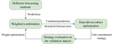
Figure 1: Integrated forecasting and optimization framework.

II-D Surrogate Model to Speed up the Weight Optimization

We first establish the proposed surrogate model and then introduce how to optimize the weight efficiently using the surrogate model.

II-D1 Multilayer Perceptron-Based Surrogate Model

Fig. 2 illustrates the proposed surrogate model, which adopts a multilayer perceptron neural network to capture the mapping from predictions and weight to performance, i.e., the cost of robust UC. The predictions $(\hat{\mathbf{U}}^{(m)};m\in\mathcal{M})$ have a high dimension in the UC problem, so we first apply principal component analysis (PCA) [23] for dimensionality reduction. Then the result becomes part of the inputs of the neural network. Because the weight $w=(w^{(m)};m\in\mathcal{M})$ satisfies $\sum_{m\in\mathcal{M}}w^{(m)}=1$, the first $|\mathcal{M}|-1$ weight components are input into the neural network, where $|\mathcal{M}|$ denotes the number of elements in $\mathcal{M}$. The inputs from the predictions and the weight are concatenated and scaled before being processed by the neural network. The rectified linear unit (ReLU) activation function is used in the neural network, which returns $v:=\max\{0,s\}$ for input scalar $s$. The neural network output is the optimal cost of robust UC, which is also scaled. Once trained, the proposed surrogate model can predict the cost based on the prediction and weight data.

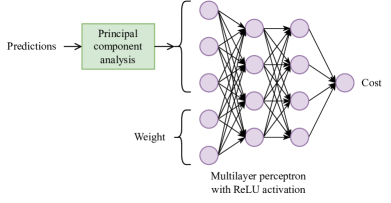
Figure 2: The proposed surrogate model.

II-D2 MILP-Based Weight Optimization

We model the proposed surrogate model via mixed-integer linear constraints. Linear constraints model PCA, scaling, and linear combination. The ReLU activation function $v=\max\{0,s\}$ is equivalent to the following group of constraints [24]:

$$0\leq v\leq Mz,$$ (4a)

$$s\leq v\leq s+M(1-z),$$ (4b)

where $z$ is an auxiliary binary variable and $M$ is a large positive constant. When $z=0$, (4a) forces $v=0$ and (4b) implies $v\geq s$; when $z=1$, (4b) shows $v=s$ and by (4a) we have $v\geq 0$. Therefore, the ReLU activation function is equivalently modeled by the linear constraints in (4) with binary variables. The surrogate model is then formulated as mixed-integer linear constraints.

To efficiently optimize the weight, a MILP problem is solved to minimize the output of the neural network, where the day-ahead prediction data are used, the weight satisfies $w\geq 0$ and $\sum_{m\in\mathcal{M}}w^{(m)}=1$, and linear constraints with binary variables capture the surrogate model. The optimal weight value is used in the integrated forecasting and optimization framework.

III Data-Driven Two-Stage Robust Unit Commitment with Statistical Guarantees

In this section, we first establish the robust UC problem and then construct the uncertainty set, which is later reconstructed using the problem information. The solution algorithm is introduced in the end.

III-A Robust Unit Commitment Formulation

As introduced in Section II-B, the robust UC problem has the compact form in (2). Now we specify the components of this problem. The pre-dispatch variable $x=(\theta_{gt},\theta_{gt}^{\pm},p_{gt},r_{gt}^{\pm};g\in\mathcal{G},t\in\mathcal{T})$, where $\mathcal{G}$ and $\mathcal{T}$ are the index sets of generators and periods, respectively. For generator $g$ in period $t$, $\theta_{gt}$, $\theta_{gt}^{+}$, and $\theta_{gt}^{-}$ are the binary variables for the on, startup, and shutdown states; $p_{gt}$ is the day-ahead scheduled power output; $r_{gt}^{+}$ and $r_{gt}^{-}$ are the upward and downward reserve power, respectively. The pre-dispatch cost is given by

$$f(x)=\sum_{t\in\mathcal{T}}\sum_{g\in\mathcal{G}}\left(o_{g}^{+}\theta_{gt}^{+}+o_{g}^{-}\theta_{gt}^{-}+\rho_{g}p_{gt}+\gamma_{g}^{+}r_{gt}^{+}+\gamma_{g}^{-}r_{gt}^{-}\right),$$ (5)

where $o_{g}^{\pm}$, $\rho_{g}$, and $\gamma_{g}^{\pm}$ are cost coefficients. The pre-dispatch feasible region is defined as follows:

$$\mathcal{X}=\left\{x=(\theta_{gt},\theta_{gt}^{\pm},p_{gt},r_{gt}^{\pm};g\in\mathcal{G},t\in\mathcal{T})~{}\right|$$

$$\sum_{g\in\mathcal{G}}p_{gt}=\sum_{i\in\mathcal{I}}\hat{u}_{it},\forall t\in\mathcal{T},$$ (6a)

$$-S_{l}\leq\sum_{g\in\mathcal{G}}\pi_{gl}p_{gt}-\sum_{i\in\mathcal{I}}\pi_{il}\hat{u}_{it}\leq S_{l},\forall l\in\mathcal{L},\forall t\in\mathcal{T},$$ (6b)

$$\theta_{gt},\theta_{gt}^{+},\theta_{gt}^{-}\in\{0,1\},\forall g\in\mathcal{G},\forall t\in\mathcal{T},$$ (6c)

$$\sum_{\tau=t}^{t+T_{g}^{+}-1}\theta_{g\tau}\geq T_{g}^{+}\theta_{gt}^{+},1\leq t\leq T-T_{g}^{+}+1,\forall g\in\mathcal{G},$$ (6d)

$$\sum_{\tau=t}^{T}(\theta_{g\tau}-\theta_{gt}^{+})\geq 0,T-T_{g}^{+}+2\leq t\leq T,\forall g\in\mathcal{G},$$ (6e)

$$\sum_{\tau=t}^{t+T_{g}^{-}-1}(1-\theta_{g\tau})\geq T_{g}^{-}\theta_{gt}^{-},1\leq t\leq T-T_{g}^{-}+1,\forall g\in\mathcal{G},$$ (6f)

$$\sum_{\tau=t}^{T}(1-\theta_{g\tau}-\theta_{gt}^{-})\geq 0,T-T_{g}^{-}+2\leq t\leq T,\forall g\in\mathcal{G},$$ (6g)

$$\theta_{gt}-\theta_{g(t-1)}=\theta_{gt}^{+}-\theta_{gt}^{-},\forall g\in\mathcal{G},\forall t\in\mathcal{T},$$ (6h)

$$\theta_{gt}^{+}+\theta_{gt}^{-}\leq 1,\forall g\in\mathcal{G},\forall t\in\mathcal{T},$$ (6i)

$$0\leq r_{gt}^{+}\leq R_{g}^{+}\theta_{gt},0\leq r_{gt}^{-}\leq R_{g}^{-}\theta_{gt},\forall g\in\mathcal{G},\forall t\in\mathcal{T},$$ (6j)

$$\underline{P}_{g}\theta_{gt}+r_{gt}^{-}\leq p_{gt}\leq\overline{P}_{g}\theta_{gt}-r_{gt}^{+},\forall g\in\mathcal{G},\forall t\in\mathcal{T},$$ (6k)

$$(p_{gt}+r_{gt}^{+})-(p_{g(t-1)}-r_{g(t-1)}^{-})\leq K_{g}^{+}\theta_{g(t-1)}$$

$$+K_{g}^{U}\theta_{gt}^{+},\forall g\in\mathcal{G},2\leq t\leq T,$$ (6l)

$$-(p_{gt}-r_{gt}^{-})+(p_{g(t-1)}+r_{g(t-1)}^{+})\leq K_{g}^{-}\theta_{gt}$$

$$\left.+K_{g}^{D}\theta_{gt}^{-},\forall g\in\mathcal{G},2\leq t\leq T\right\}.$$ (6m)

The power balance of the transmission network is stipulated in (6a), where $\hat{u}_{it}$ is the day-ahead prediction of the load power. In (6b), $\mathcal{L}$ is the index set of transmission lines; $S_{l}$ is the power capacity of line $l$; $\pi_{gl}$ and $\pi_{il}$ are the power transfer distribution factors. Thus, (6b) bounds the line flow in the DC power flow model. Binary variables are set in (6c). Constraints (6d)-(6g) are for the minimum up time $T_{g}^{+}$ and minimum down time $T_{g}^{-}$ of generators [25]. The generator state change is modeled in (6h) and the simultaneous startup and shutdown of a generator is prohibited in (6i). Constraint (6j) contains bounds $R_{g}^{\pm}$ for the upward and downward reserve power. The minimum and maximum outputs of generators, i.e., $\underline{P}_{g}$ and $\overline{P}_{g}$ for generator $g$, are stipulated in (6k). For generator $g$, $K_{g}^{+}$ and $K_{g}^{-}$ are the maximum upward and downward ramp values in a period; $K_{g}^{U}$ and $K_{g}^{D}$ are the maximum increase and decrease of power if the generator startups or shutdowns in a period. Thus, constraints (6l) and (6m) are the bounds for the change in generator power over a period.

The construction of the uncertainty set $\mathcal{U}$ is deferred and will be addressed in Sections III-B and III-C. In the re-dispatch stage, the variable is $y=(p_{gt}^{\pm};g\in\mathcal{G},t\in\mathcal{T})$, where $p_{gt}^{+}$ and $p_{gt}^{-}$ are the upward and downward power adjustments of generator $g$ in period $t$, respectively. The re-dispatch cost function is the total power adjustment cost, i.e.,

$$h(y)=\sum\nolimits_{t\in\mathcal{T}}\sum\nolimits_{g\in\mathcal{G}}\left(\rho_{g}^{+}p_{gt}^{+}+\rho_{g}^{-}p_{gt}^{-}\right),$$ (7)

where $\rho_{g}^{+}$ and $\rho_{g}^{-}$ are cost coefficients. The re-dispatch feasible region $\mathcal{Y}(x,u)$ depends on the pre-dispatch decision $x$ and the realization $u=(u_{it};i\in\mathcal{I},t\in\mathcal{T})$ of uncertain load:

$$\mathcal{Y}(x,u)=\left\{y=(p_{gt}^{\pm};g\in\mathcal{G},t\in\mathcal{T})~{}\right|$$

$$\sum\nolimits_{g\in\mathcal{G}}(p_{gt}+p_{gt}^{+}-p_{gt}^{-})=\sum\nolimits_{i\in\mathcal{I}}u_{it},\forall t\in\mathcal{T},$$ (8a)

$$-S_{l}\leq\sum\nolimits_{g\in\mathcal{G}}\pi_{gl}(p_{gt}+p_{gt}^{+}-p_{gt}^{-})-\sum\nolimits_{i\in\mathcal{I}}\pi_{il}u_{it}$$

$$\leq S_{l},\forall l\in\mathcal{L},\forall t\in\mathcal{T},$$ (8b)

$$\left.0\leq p_{gt}^{+}\leq r_{gt}^{+},0\leq p_{gt}^{-}\leq r_{gt}^{-},\forall g\in\mathcal{G},\forall t\in\mathcal{T}\right\}.$$ (8c)

In (8), constraint (8a) is for the power balance of the network. The transmission line flow constraints are in (8b). The power adjustments of the generators are bounded by the reserve power in (8c).

According to the formulations of $f(x)$ and $h(y)$ in (5) and (7), the two functions are linear. Equation (8) shows that the constraints that define $\mathcal{Y}(x,u)$ are linear in $x$ and $u$. Therefore, the compact form of the robust UC problem can be further written as follows:

$$\min\nolimits_{x\in\mathcal{X}}\left\{C^{\top}x+\max\nolimits_{u\in\mathcal{U}}\min\nolimits_{y:Ay\geq Bx+Du+E}F^{\top}y\right\},$$ (9)

where $A$, $B$, $C$, $D$, $E$, and $F$ are coefficient matrices and vectors.

III-B Data-Driven Uncertainty Set and Statistical Guarantees

The possible realization values of the uncertain load $u$ constitute a set $\mathcal{U}_{0}$ as follows:

$$\mathcal{U}_{0}=\left\{u~{}\middle|~{}\underline{U}\leq u\leq\overline{U},\underline{E}\leq u-\hat{u}\leq\overline{E}\right\},$$ (10)

where $\underline{U}$ and $\overline{U}$ are the lower and upper bounds for $u$; $\underline{E}$ and $\overline{E}$ are the lower and upper bounds for the forecast error of $u$. $\mathcal{U}_{0}$ contains all the possible values of $u$, so $\Pr[u\in\mathcal{U}_{0}]=1$.

According to the analysis in Section II-B, we need to construct an uncertainty set $\mathcal{U}_{1}\subset\mathcal{U}_{0}$ such that $\Pr[u\in\mathcal{U}_{1}]\geq 1-\varepsilon$, where the materials we have include prediction $\hat{u}$ and historical forecast error $e_{1:N}:=(e_{1},e_{2},\dots,e_{N})$ in the training dataset ($e_{n}$ is the column vector reshaping $\mathbf{E}_{1:T}^{(n)}(w)$). We assume that the daily load forecast errors are i.i.d. continuous random variables. Our plan is first to construct a set $\mathcal{E}$ for the uncertain forecast error $e:=u-\hat{u}$ so that $\Pr[e\in\mathcal{E}]\geq 1-\varepsilon$, followed by letting

$$\mathcal{U}_{1}:=\{u\in\mathcal{U}_{0}~{}|~{}u-\hat{u}\in\mathcal{E}\}.$$ (11)

Clearly, such $\mathcal{U}_{1}$ satisfies $\mathcal{U}_{1}\subset\mathcal{U}_{0}$ and $\Pr[u\in\mathcal{U}_{1}]\geq 1-\varepsilon$, so the uncertainty set construction problem comes down to finding a set $\mathcal{E}$ such that $\Pr[e\in\mathcal{E}]\geq 1-\varepsilon$, based on the historical data $e_{1:N}$.

Since $e_{1:N}$ are random variables, the set $\mathcal{E}$ constructed using $e_{1:N}$ is also random, and so is the event $\Pr[e\in\mathcal{E}]\geq 1-\varepsilon$. Therefore, instead of directly attempting $\Pr[e\in\mathcal{E}]\geq 1-\varepsilon$, we consider the following statistical guarantee:

$$\mathbb{P}^{N}[\Pr[e\in\mathcal{E}]\geq 1-\varepsilon]\geq 1-\delta,$$ (12)

where $\mathbb{P}$ is the underlying distribution of $e_{n},n=1,2,\dots,N$; $\mathbb{P}^{N}$ denotes the $N$ times distribution product of $\mathbb{P}$, which models the uncertainty of historical data and $\mathcal{E}$; $\delta$ is a probability tolerance parameter. Thus, equation (12) means that the probability of the random event $\Pr[e\in\mathcal{E}]\geq 1-\varepsilon$ is at least $1-\delta$. The parameters $\varepsilon$ and $\delta$ jointly control the conservative degree of the robust UC problem.

To achieve the statistical guarantee (12), we adopt the data-driven uncertainty set proposed in [11] to establish $\mathcal{E}$, whose procedure and statistical guarantee are summarized in Theorem 1. The idea is to pull two disjoint groups from the dataset. The first group determines the shape of $\mathcal{E}$, where an ellipsoid is established based on the sample mean and covariance to consider the correlation. The second group is for the size of $\mathcal{E}$, where the differences of the points from the ellipsoid center are measured and sorted to provide a threshold, and the independence of the two data groups forms the foundation of the statistical guarantees.

Theorem 1 (Uncertainty set construction and statistical guarantee)

Select two disjoint groups from $e_{1:N}$. Denote their realizations by $e_{1:N_{1}}^{(1)}$ and $e_{1:N_{2}}^{(2)}$, where $N_{1}+N_{2}\leq N$ and $N_{2}\geq\log_{1-\varepsilon}\delta$. Let

$$\mu:=\frac{1}{N_{1}}\sum_{n=1}^{N_{1}}e_{n}^{(1)},$$ (13a)

$$\Sigma:=\frac{1}{N_{1}-1}\sum_{n=1}^{N_{1}}\left(e_{1:N_{1}}^{(1)}-\mu 1_{1\times N_{1}}\right)\left(e_{1:N_{1}}^{(1)}-\mu 1_{1\times N_{1}}\right)^{\top}.$$ (13b)

In other words, $\mu$ and $\Sigma$ are the sample mean and the sample covariance matrix in the first dataset $e_{1:N_{1}}^{(1)}$. Assume $\Sigma$ is invertible. Define function $a(e):=(e-\mu)^{\top}\Sigma^{-1}(e-\mu)$. Let

$$n_{N}^{*}:=\min\left\{n\in\mathbb{N}~{}\middle|~{}\sum\nolimits_{m=0}^{n-1}C_{N}^{m}(1-\varepsilon)^{m}\varepsilon^{N-m}\geq 1-\delta\right\},$$ (14)

where $C_{N}^{m}$ denotes the binomial coefficient of $N$ choose $m$. Let $\alpha$ be the $n_{N_{2}}^{*}$-th smallest value in $a(e_{1}^{(2)}),a(e_{2}^{(2)}),\dots,a(e_{N_{2}}^{(2)})$. Define the set $\mathcal{E}$ as

$$\mathcal{E}:=\left\{e~{}\middle|~{}(e-\mu)^{\top}\Sigma^{-1}(e-\mu)\leq\alpha\right\}.$$ (15)

Then the statistical guarantee (12) holds. Moreover, if $\mathcal{U}=\mathcal{U}_{1}$ defined in (11) is used in the robust UC problem (2) and $x_{0}:=x_{\mathcal{U}_{1}}^{*}$ is an optimal solution, then

$$\mathbb{P}^{N}[\Pr[O\leq O_{x_{0}}\leq O_{\mathcal{U}_{1}}]\geq 1-\varepsilon]\geq 1-\delta.$$ (16)

Theorem 1 gives a method to generate the uncertainty set $\mathcal{U}_{1}$ and approximate problem (1) with confidence $1-\delta$. The proof of Theorem 1 can be found in Appendix B.

III-C Uncertainty Set Reconstruction

The uncertainty set $\mathcal{U}_{1}$ obtained in Theorem 1 guarantees robustness with confidence $1-\delta$, but it can be conservative. Our goal in this subsection is to mitigate the conservativeness by reconstructing the uncertainty set. The construction of $\mathcal{U}_{1}$ uses only the prediction and historical forecast error but does not involve any information on the UC problem. In the following, we integrate the problem information into the reconstruction.

We illustrate the basic idea in Fig. 3. Ellipsoid 1 denotes $\mathcal{U}_{1}$ constructed in Section III-B. The worst-case scenario in ellipsoid 1 is marked as a blue star, which reaches the highest cost in it. Consider the range where the cost is not higher than the blue star, then we obtain polyhedron 1 in Fig. 3. This range is a polyhedron because of the linear structure in problem (9). Polyheron 1 contains ellipsoid 1 and the blue star is also a worst-case scenario in polyheron 1. Moreover, polyhedron 1 may include more data points than ellipsoid 1 and thus be conservative, which indicates that polyhedron 1 can be shrunk into polyhedron 2 according to the desired probability guarantee thresholds. Hopefully, the worst-case scenario in polyhedron 2 has a smaller cost than the blue star, and the conservativeness is mitigated.

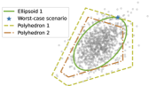
Figure 3: The basic idea of uncertainty set reconstruction.

Now we explain the reconstruction formally. Recall from Lemma 1 that when $(x^{*},\eta^{*})$ is optimal for the chance-constrained problem (1), the uncertainty set $\mathcal{U}^{*}$ defined in (3) can equivalently transform problem (1) into (2). Ideally, $\mathcal{U}^{*}$ is used as the uncertainty set to eliminate conservativeness. However, it is impractical because $(x^{*},\eta^{*})$ is unknown. To this end, $\mathcal{U}^{*}$ is approximated using the data we have. Suppose $x_{0}$ is a feasible solution, then we can estimate its performance $O_{x_{0}}$ in a historical dataset and construct an uncertainty set using $(x,\eta)=(x_{0},O_{x_{0}}-f(x_{0}))$. This idea is refined to maintain the statistical guarantees in Theorem 2.

Theorem 2 (Uncertainty set reconstruction)

Suppose $e_{1:N_{3}}^{(3)}$ is a subgroup of $e_{1:N}$ and $N_{3}\geq\log_{1-\varepsilon}\delta$. Assume that the solution $x_{0}$ is independent of $e_{1:N_{3}}^{(3)}$. Define function $b(u):=\min_{y\in\mathcal{Y}(x_{0},u)}h(y)$. Define $n_{N_{3}}^{*}$ according to (14). Let $\beta$ be the $n_{N_{3}}^{*}$-th smallest value in $b(\hat{u}+e_{1}^{(3)}),b(\hat{u}+e_{2}^{(3)}),\dots,b(\hat{u}+e_{N_{3}}^{(3)})$. Define the uncertainty set

$$\mathcal{U}_{2}:=\left\{u\in\mathcal{U}_{0}~{}\middle|~{}\min\nolimits_{y\in\mathcal{Y}(x_{0},u)}h(y)\leq\beta\right\}.$$ (17)

Let $x_{1}:=x_{\mathcal{U}_{2}}^{*}$ be optimal in problem (2) with $\mathcal{U}=\mathcal{U}_{2}$. Then the following statistical guarantees hold:

$$\mathbb{P}^{N}[\Pr[u\in\mathcal{U}_{2}]\geq 1-\varepsilon]\geq 1-\delta,$$ (18a)

$$\mathbb{P}^{N}[\Pr[O\leq O_{x_{1}}\leq O_{\mathcal{U}_{2}}\leq f(x_{0})+\beta]\geq 1-\varepsilon]\geq 1-\delta.$$ (18b)

In Theorem 2, the shape of the new uncertainty set is formed based on both the old solution and the UC problem, whereas the size $\beta$ is determined by the evaluations on an independent dataset so that the statistical guarantees remain valid. The conclusion indicates that the reconstruction of the uncertainty set will lead to a new solution probably better than the old one, represented by $O_{x_{1}}\leq f(x_{0})+\beta$. The proof of Theorem 2 can be found in Appendix C.

III-D Solution Algorithm

$\mathcal{U}_{0}$ defined in (10) is polyhedral. According to (11) and (15),

$$\mathcal{U}_{1}=\{u\in\mathcal{U}_{0}~{}|~{}(u-\hat{u}-\mu)^{\top}\Sigma^{-1}(u-\hat{u}-\mu)\leq\alpha\},$$

is the intersection of an ellipsoid and a polyhedron. Using the compact form of the robust UC problem in (9), $\mathcal{U}_{2}$ in (17) can be further written as follows:

$$\mathcal{U}_{2} =\{u\in\mathcal{U}_{0}~{}|~{}\exists y\in\mathcal{Y}(x_{0},u),~{}\mbox{s.t.}~{}h(y)\leq\beta\}$$

$$=\{u\in\mathcal{U}_{0}~{}|~{}\exists y,~{}\mbox{s.t.}~{}Ay\geq Bx_{0}+Du+E,F^{\top}y\leq\beta\},$$

which shows that $\mathcal{U}_{2}$ is polyhedral. Therefore, the two uncertainty sets are polyhedral or ellipsoidal. Problem (9) with these uncertainty sets can be effectively solved by the column-and-constraint generation (C&CG) algorithm [26], which is omitted here for the sake of conciseness.

The solution procedure for the robust UC problem considering uncertainty set reconstruction is summarized in Algorithm 1. The historical dataset is divided into two groups. The first group forms the first ellipsoidal uncertainty set and leads to a solution $x_{0}$. Then the reconstruction procedure in Theorem 2 is performed to obtain an improved uncertainty set, resulting in the final solution $x_{1}$. Since the two datasets are independent, the statistical guarantees in (18) are maintained.

Input: Parameters of (9); $\varepsilon$; $\delta$; $\mathcal{U}_{0}$; $\hat{u}$; $e_{1:N}$; $N_{2}$

Output: UC strategy $x_{1}$

1 $N_{1}\leftarrow N-N_{2}$

2 Divide $e_{1:N}$ into $e_{1:N_{1}}^{(1)}$ and $e_{1:N_{2}}^{(2)}$

3 Calculate $\mu$ and $\Sigma$ according to (13)

4 $\alpha\leftarrow\max\{(e_{n}^{(1)}-\mu)^{\top}\Sigma^{-1}(e_{n}^{(1)}-\mu)~{}|~{}n=1,2,\dots,N_{1}\}$

5 $\mathcal{U}_{1}^{\prime}\leftarrow\{u\in\mathcal{U}_{0}~{}|~{}(u-\hat{u}-\mu)^{\top}\Sigma^{-1}(u-\hat{u}-\mu)\leq\alpha\}$

6 Solve problem (9) with $\mathcal{U}=\mathcal{U}_{1}^{\prime}$ using the C&CG algorithm and obtain the optimal solution $x_{0}$

7 $b_{n}\leftarrow\min_{y:Ay\geq Bx_{0}+D(\hat{u}+e_{n}^{(2)})+E}F^{\top}y$, for $n=1,2,\dots,N_{2}$

8 Arrange $b_{n},n=1,2,\dots,N_{2}$ from small to large and get $b_{n}^{\prime},n=1,2,\dots,N_{2}$

9 $n^{*}\leftarrow\min\{n|\sum_{m=0}^{n-1}C_{N_{2}}^{m}(1-\varepsilon)^{m}\varepsilon^{N_{2}-m}\geq 1-\delta\}$

10 $\beta\leftarrow b_{n^{*}}^{\prime}$

11 $\mathcal{U}_{2}\leftarrow\{u\in\mathcal{U}_{0}|\exists y,~{}\mbox{s.t.}~{}Ay\geq Bx_{0}+Du+E,F^{\top}y\leq\beta\}$

12 Solve problem (9) with $\mathcal{U}=\mathcal{U}_{2}$ using the C&CG algorithm and return the optimal solution $x_{1}$

Algorithm 1 Solution of robust unit commitment

IV Case Studies

This section examines the proposed robust UC method using modified IEEE 30-bus and 118-bus systems. All experiments are carried out on a laptop with an Intel i7-12700H processor and 16 GB RAM. The neural network is established and trained by PyTorch 2.1.2. The MILP problems in the C&CG algorithm are solved by Gurobi 11.0.2. In the following, we first introduce the prediction data. The performance of the proposed method is then investigated in the modified IEEE 30-bus system, where different methods are compared and sensitivity analysis is performed. Finally, the modified IEEE 118-bus system is used to demonstrate the scalability of the proposed method.

IV-A Prediction Data

The hourly load data in one and a half years are extracted from the dataset in [27], based on real data in Ireland [28]. The hourly wind power data are generated according to historical weather data [29]. The load and wind data are aligned according to the date information. The dataset is divided into samples for training, validation, and testing.

We predict uncertainty using the following forecasting methods:

• M1: Forecast nodal power using local data and bidirectional long short-term memory (BiLSTM) neural network [30].

• M2: Apply federated learning between nodes and forecast using the adapted global BiLSTM model [31].

• M3: Forecast nodal power using BiLSTM networks and nodal power subprofiles [15].

• C1: Combine the predictions of M1, M2, and M3 by a weight $w$ to minimize the mean square error (MSE) on the validation dataset.

• C2: Combine the predictions of M1, M2, and M3 by a weight $w$ according to the method proposed in Section II.

The loss function used in the training is MSE. We adopt root mean square error (RMSE) and mean absolute error (MAE) to measure the test forecast errors.

The average forecast errors under different methods are shown in TABLE I. By combining three forecasting methods and optimizing the weight to minimize the MSE, C1 has the lowest forecast errors, whose RMSE is 11.1%, 7.3%, and 6.8% lower than M1, M2, and M3, respectively. It verifies that the combination of predictions is effective in improving forecast accuracy by leveraging the potential of different data sources and forecasting methods. The forecast errors of C2 are larger than those of C1 because instead of minimizing the MSE, the weight in C2 is chosen to minimize the UC cost.

TABLE I: Average Forecast Errors of Different Methods

Method	RMSE	MAE
M1	84.39	54.64
M2	80.93	52.37
M3	80.44	55.23
C1	76.14	51.26
C2 (30-bus)	76.95	52.29
C2 (118-bus)	78.72	53.80

IV-B Modified IEEE 30-Bus System

Based on the prediction data mentioned above, the integrated framework in Fig. 1 and the proposed data-driven RO method in Algorithm 1 are used for the robust UC problem. In the modified IEEE 30-bus system, there are six controllable generators and four wind farms, where $\underline{P}_{g}=(100,40,0,0,0,0)$ MW, $\overline{P}_{g}=(360,140,100,100,100,100)$ MW, and $T_{g}^{+}=T_{g}^{-}=6$ h. Other parameters are in [32].

IV-B1 Benchmark

In the benchmark case, the probability tolerance parameters are set as $\varepsilon=\delta=$ 5%. We divide the training dataset into two subsets with $N_{1}$ and $N_{2}$ data, respectively. According to Theorem 1 and Theorem 2, $N_{2}$ should be at least $59$. We set $N_{1}=212$ and $N_{2}=124$.

Based on the performance on the validation dataset, we use the first three components of PCA in the surrogate model for weight optimization. The multilayer perceptron neural network has two hidden layers, and each layer has 16 units. The neural network is trained using the Adam algorithm and the learning rate is 0.001. To help prevent overfitting, we adopt the L2 regularization technique. After about 1000 epochs, the neural network is trained.

The test day for UC is from the test dataset. The MILP problem for weight optimization is solved in 0.02 s and the result is $w=(0.28,0.23,0.49)$. The weight for M3 is the highest, reflecting that the sub-profiles are valuable in power forecasting and robust UC, which is consistent with the results in TABLE I and [15]. With the optimized weight, the UC results are obtained after 121 s, and the optimal value is $89725. The power outputs of some controllable generators are depicted in Fig. 4, including the pre-dispatch power, the reserve region, and the re-dispatch result in the worst-case scenario. The power in the re-dispatch stage is always within the reserve region.

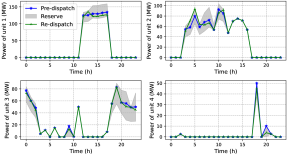
Figure 4: Power outputs of controllable generators.

IV-B2 Comparison

We use out-of-sample tests to examine the performance of the proposed method under uncertainty. Meanwhile, we compare the proposed method with the following alternative methods:

• SP: The traditional chance-constrained SP method using the estimated distribution based on historical data.

• RO1: The traditional data-driven RO method with an ellipsoidal uncertainty set that includes all data.

• RO2: The same method as RO1 except that the ellipsoidal uncertainty set includes $1-\varepsilon$ proportion of the data.

• P1: The data-driven RO method using the ellipsoidal uncertainty set with statistical guarantees.

• P2: The data-driven RO method using Algorithm 1, where the weight $w$ is optimized to minimize the MSE.

For clarity, the settings of these methods are compared in TABLE II, with results listed in TABLE III. The feasible rate is calculated using the 100 forecast error samples on the test dataset. The total cost is the real value on the test day.

TABLE II: Settings of Unit Commitment Methods for Comparison

Method	Statistical	Integrated forecasting	Uncertainty set
	guarantee	and optimization	reconstruction
SP	$\times$	$\times$	$\times$
RO1	$\times$	$\times$	$\times$
RO2	$\times$	$\times$	$\times$
P1	✓	✓	$\times$
P2	✓	$\times$	✓
Proposed	✓	✓	✓

TABLE III: Unit Commitment Results of Different Methods in the Modified IEEE 30-Bus System

Method	Objective ($)	Feasible rate	Total cost ($)	Time (s)
SP	84832	88%	82985	218
RO1	106810	100%	92652	143
RO2	97350	97%	90468	94
P1	97848	98%	89149	124
P2	90122	98%	88318	147
Proposed	89725	98%	88243	121

As TABLE III shows, SP has the lowest objective value and test total cost. However, its test feasible rate is $88$%, much lower than the desired threshold $95$%, which shows that SP lacks robustness. The other five methods are RO-based and their test feasible rates all meet the requirement. However, RO1 is rather conservative and has the highest objective value and test total cost. RO2 is a traditional data-driven RO method with no statistical guarantees, which shows its theoretical limitation. P1, P2, and the proposed method have statistical guarantees, and the proposed method achieves the lowest optimal objective and test total cost among them. Using uncertainty set reconstruction, the objective decreases $8.30$%. The integrated forecasting and optimization framework also contributes to improving the objective. The computation time is acceptable for all the methods. Therefore, TABLE III verifies that the proposed method is effective. It outperforms other methods when considering both robustness and optimality. Moreover, the proposed weight optimization and uncertainty set reconstruction processes help improve the performance.

To visualize different uncertainty sets, we consider a special case of two random loads. The uncertainty sets are projected onto a two-dimensional plane. The projections of the uncertainty sets are drawn in Fig. 5. To emphasize the impact of uncertainty set construction and reconstruction, the weight $w$ is fixed to that of C1. The black polygon is the projection of $\mathcal{U}_{0}$ defined in (10). All other uncertainty sets are the intersections of $\mathcal{U}_{0}$ and ellipsoids or polyhedrons. The projected uncertainty set of RO1 is framed by an ellipse that includes all the data points. RO2’s ellipse has the same shape and center but only contains $95$% data points. RO2 does not have a statistical guarantee for its out-of-sample performance. P1 has a larger uncertainty set than RO2 to maintain the statistical guarantees, but P1 does not reconstruct the uncertainty set to decrease the conservativeness. Proposed_1 and Proposed_2 are the projections of the first and second uncertainty sets of the proposed method ($\mathcal{U}_{1}^{\prime}$ and $\mathcal{U}_{2}$ in Algorithm 1), respectively. Proposed_1 is framed by an ellipse similar to that of P1. After the reconstruction, Proposed_2 no longer includes the right part of the ellipse, so it omits some bad scenarios in the UC problem. Meanwhile, Proposed_2 includes other regions with a relatively low cost, so the data points in it are still enough for the statistical guarantees. In this way, the proposed uncertainty set mitigates conservativeness while maintaining statistical guarantees.

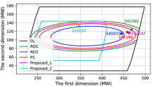
Figure 5: Projections of uncertainty sets onto a two-dimensional plane in the case of two random loads, where the projections of worst-case scenarios within these uncertainty sets are marked by stars, with the costs ($) labeled.

IV-B3 Sensitivity Analysis

We investigate the impacts of weight $w$, the number of data points $N_{2}$, and the probability tolerance parameters $\varepsilon$ and $\delta$ for sensitivity analysis. The total costs under different values of weight $w$ are depicted in Fig. 6. As Fig. 6 shows, there is a valley in the middle of the weight’s feasible region, which means that the combination of the three kinds of predictions has the best performance. The optimal weight computed by the MILP problem of the surrogate model lies in the center region of the valley and achieves a low total cost, showing the effectiveness of the surrogate model.

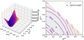
Figure 6: Total costs under different weights. (Because $w^{(2)}=1-w^{(0)}-w^{(1)}$, we only draw the relationship between the total cost, $w^{(0)}$, and $w^{(1)}$, where the weight satisfies $w^{(0)}\geq 0$, $w^{(1)}\geq 0$, and $w^{(0)}+w^{(1)}\leq 1$.)

To demonstrate the requirements of statistical guarantees, we investigate the number and proportion of the $N_{2}$ data points outside the uncertainty set when $N_{2}$, $\varepsilon$, and $\delta$ vary. In the benchmark case, $N_{2}=124$ and $\varepsilon=\delta=5$%. As $N_{2}$ increases, the number of points outside steps up because it must be an integer. The proportion of points outside becomes closer to $\varepsilon=5$% under a larger $N_{2}$. This means that the statistical guarantees are easier to retain in a larger dataset. When $\varepsilon$ increases under fixed $N_{2}$ and $\delta$, the proportion of points outside the uncertainty set increases but never exceeds $\varepsilon$, which indicates that more data points should be included in the uncertainty set than the specified proportion to achieve a statistical guarantee of out-of-sample performance. As $\delta$ increases, the proportion of points outside increases.

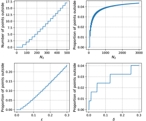
Figure 7: Proportion of points outside the proposed uncertainty set under different settings.

Fig. 8 shows the results of the optimal value and the test feasible rate under different $\varepsilon$. As $\varepsilon$ increases, the robust degree weakens, and therefore the objective value and the test feasible rate both decrease. When $\varepsilon\in[0.05,0.17]$, the test feasible rate is larger than $1-\varepsilon$, reflecting the effectiveness of the probability guarantee. Approximately speaking, the test feasible rate decreases linearly as $\varepsilon$ increases when $\varepsilon\geq 0.05$.

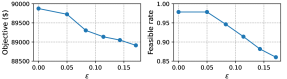
Figure 8: Results under different $\varepsilon$.

The impacts of the probability threshold $\delta$ are shown in Fig. 9. As $\delta$ increases, the confidence in the chance constraint $\Pr[u\in\mathcal{U}]\geq 1-\varepsilon$ decreases, so the results become less conservative, leading to decreases in the objective value and test feasible rate. When $\delta\leq 0.13$, the test feasible rate exceeds $1-\varepsilon=95$%. However, when $\delta$ is too large, the desired probability $1-\varepsilon$ is no longer satisfied on the test dataset. Therefore, we recommend a small value for parameter $\delta$.

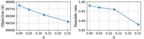
Figure 9: Results under different $\delta$.

IV-C Modified IEEE 118-Bus System

We use a modified IEEE 118-bus system with 54 controllable generators and four wind farms to show the scalability. The parameter settings are $\varepsilon=\delta=$ 5%, $N_{1}=212$, and $N_{2}=124$. More details can be found in [32]. The UC results under different methods are shown in TABLE IV. The method relationships are similar to those in the modified IEEE 30-bus system. In addition, the computation time increases but is still acceptable for day-ahead UC. We also test the computation efficiency under different numbers of random loads in the modified IEEE 118-bus system, as shown in Table V. These results verify the scalability of the proposed method.

TABLE IV: Unit Commitment Results of Different Methods in the Modified IEEE 118-Bus System

Method	Objective ($)	Feasible rate	Total cost ($)	Time (s)
SP	2061915	84%	2055123	1638
RO1	2096428	100%	2069461	256
RO2	2086813	100%	2064276	634
P1	2092717	100%	2068213	1304
P2	2066737	100%	2058488	1076
Proposed	2065591	100%	2056996	763

TABLE V: Computation Efficiency in the Modified IEEE 118-Bus System

Number of random loads	25	21	17	13
Number of iterations	23	21	21	18
Computation time (s)	763	600	551	391

V Conclusion

To enhance out-of-sample performance and ensure robustness, this paper develops a new data-driven two-stage robust UC method. The proposed integrated forecasting and optimization framework combines different predictions using weights optimized based on UC performance outcomes. A surrogate model is established to accelerate the weight optimization process. In the two-stage robust UC, the uncertainty set is constructed from data to have statistical guarantees, and it is then reconstructed using the information from the optimization problem to reduce conservativeness. Comparative analysis on modified IEEE 30-bus and 118-bus systems demonstrates that the proposed method surpasses traditional SP and RO methods in balancing robustness with out-of-sample performance. The case studies also show that the computational complexity of the proposed method is comparable to that of traditional RO methods, making it scalable. Future work could explore multi-stage robust UC with statistical guarantees.

Appendix A Proof of Lemma 1

1) Prove that $O=O_{x^{*}}\leq O_{x_{\mathcal{U}}^{*}}\leq O_{\mathcal{U}}$ when $\Pr[u\in\mathcal{U}]\geq 1-\varepsilon$:

Because $(x^{*},\eta^{*})$ is optimal in (1), we have $O=O_{x^{*}}$ and

$$O =f(x^{*})+\min\left\{\eta~{}\middle|~{}\Pr\left[\min_{y\in\mathcal{Y}(x^{*},u)}h(y)\leq\eta\right]\geq 1-\varepsilon\right\}$$

$$\leq f(x_{\mathcal{U}}^{*})+\min\left\{\eta~{}\middle|~{}\Pr\left[\min_{y\in\mathcal{Y}(x_{\mathcal{U}}^{*},u)}h(y)\leq\eta\right]\geq 1-\varepsilon\right\}$$

$$=O_{x_{\mathcal{U}}^{*}}.$$

Let

$$\eta_{\mathcal{U}}^{*}=\max\nolimits_{u\in\mathcal{U}}\min\nolimits_{y\in\mathcal{Y}(x_{\mathcal{U}}^{*},u)}h(y).$$

Then

$$\Pr\left[\min\nolimits_{y\in\mathcal{Y}(x_{\mathcal{U}}^{*},u)}h(y)\leq\eta_{\mathcal{U}}^{*}\right]\geq\Pr[u\in\mathcal{U}]\geq 1-\varepsilon.$$

Therefore,

$$O_{x_{\mathcal{U}}^{*}} =f(x_{\mathcal{U}}^{*})+\min\left\{\eta~{}\middle|~{}\Pr\left[\min_{y\in\mathcal{Y}(x_{\mathcal{U}}^{*},u)}h(y)\leq\eta\right]\geq 1-\varepsilon\right\}$$

$$\leq f(x_{\mathcal{U}}^{*})+\eta_{\mathcal{U}}^{*}=f(x_{\mathcal{U}}^{*})+\max_{u\in\mathcal{U}}\min_{y\in\mathcal{Y}(x_{\mathcal{U}}^{*},u)}h(y)=O_{\mathcal{U}},$$

where the last equation follows from the optimality of $x_{\mathcal{U}}^{*}$ in (2). Hence, $O=O_{x^{*}}\leq O_{x_{\mathcal{U}}^{*}}\leq O_{\mathcal{U}}$.

2) Prove that $\Pr[u\in\mathcal{U}^{*}]\geq 1-\varepsilon$ and $O=O_{\mathcal{U}^{*}}$:

By the feasibility of $(x^{*},\eta^{*})$ in (1), we have

$$\Pr[u\in\mathcal{U}^{*}]=\Pr\left[\min\nolimits_{y\in\mathcal{Y}(x^{*},u)}h(y)\leq\eta^{*}\right]\geq 1-\varepsilon,$$

and then $O\leq O_{\mathcal{U}^{*}}$ by the previous conclusion. According to the definition of $\mathcal{U}^{*}$ in (3), $\min_{y\in\mathcal{Y}(x^{*},u)}h(y)\leq\eta^{*}$ for any $u\in\mathcal{U}^{*}$. Therefore,

$$O_{\mathcal{U}^{*}} =\min\nolimits_{x\in\mathcal{X}}\left\{f(x)+\max\nolimits_{u\in\mathcal{U}^{*}}\min\nolimits_{y\in\mathcal{Y}(x,u)}h(y)\right\}$$

$$\leq f(x^{*})+\max\nolimits_{u\in\mathcal{U}^{*}}\min\nolimits_{y\in\mathcal{Y}(x^{*},u)}h(y)$$

$$\leq f(x^{*})+\eta^{*}=O.$$

This completes the proof.

Appendix B Proof of Theorem 1

The function $a(e)$ is a continuous random variable, where $e$ follows the distribution $\mathbb{P}$. Therefore, the assumptions of Theorem 1 in [11] are satisfied, and then its conclusion holds, i.e., $\mathcal{E}$ satisfies the statistical guarantee (12).

Because $u\in\mathcal{U}_{0}$ must hold, we have $u-\hat{u}=e\in\mathcal{E}\iff u\in\mathcal{U}_{1}$. Combine it with Lemma 1, then

$$\Pr[e\in\mathcal{E}]\geq 1-\varepsilon \iff\Pr[u\in\mathcal{U}_{1}]\geq 1-\varepsilon$$

$$\implies O\leq O_{x_{0}}\leq O_{\mathcal{U}_{1}}.$$

Hence, (16) follows from (12), which completes the proof.

Appendix C Proof of Theorem 2

1) Prove (18a):

According to linear programming theory [33], the function $b(\hat{u}+e)$ in $e$ is continuous on the closed set

$$\left\{e~{}\middle|~{}\min\nolimits_{y\in\mathcal{Y}(x_{0},\hat{u}+e)}h(y)<+\infty\right\}$$

$$= \left\{e~{}\middle|~{}\mathcal{Y}(x_{0},\hat{u}+e)\neq\varnothing\right\}$$

$$= \left\{e~{}\middle|~{}\exists y,~{}\mbox{s.t.}~{}Ay\geq Bx_{0}+D(\hat{u}+e)+E\right\}.$$

When $\beta=+\infty$, $\mathcal{U}_{2}=\mathcal{U}_{0}$ and (18a) holds. For the finite case, Lemma 3 and Theorem 1 in [11] can be applied to $b(\hat{u}+e)$ to obtain (18a).

2) Prove (18b):

Similar to the proof of Theorem 1, the statistical guarantee (18a) implies

$$\mathbb{P}^{N}[\Pr[O\leq O_{x_{1}}\leq O_{\mathcal{U}_{2}}]\geq 1-\varepsilon]\geq 1-\delta.$$

In addition,

$$O_{\mathcal{U}_{2}} =\min\nolimits_{x\in\mathcal{X}}\left\{f(x)+\max\nolimits_{u\in\mathcal{U}_{2}}\min\nolimits_{y\in\mathcal{Y}(x,u)}h(y)\right\}$$

$$\leq f(x_{0})+\max\nolimits_{u\in\mathcal{U}_{2}}\min\nolimits_{y\in\mathcal{Y}(x_{0},u)}h(y)\leq f(x_{0})+\beta,$$

where the last inequality follows from (17), so (18b) holds.

References

- [1] M. Paturet, U. Markovic, S. Delikaraoglou, E. Vrettos, P. Aristidou, and G. Hug, “Stochastic unit commitment in low-inertia grids,” IEEE Transactions on Power Systems, vol. 35, no. 5, pp. 3448–3458, 2020.
- [2] H. Xiong, Y. Shi, Z. Chen, C. Guo, and Y. Ding, “Multi-stage robust dynamic unit commitment based on pre-extended-fast robust dual dynamic programming,” IEEE Transactions on Power Systems, vol. 38, no. 3, pp. 2411–2422, 2022.
- [3] B. Zhou, J. Fang, X. Ai, Y. Zhang, W. Yao, Z. Chen, and J. Wen, “Partial-dimensional correlation-aided convex-hull uncertainty set for robust unit commitment,” IEEE Transactions on Power Systems, vol. 38, no. 3, pp. 2434–2446, 2023.
- [4] C. Ju, T. Ding, W. Jia, C. Mu, H. Zhang, and Y. Sun, “Two-stage robust unit commitment with the cascade hydropower stations retrofitted with pump stations,” Applied Energy, vol. 334, p. 120675, 2023.
- [5] W. Wang, A. Danandeh, B. Buckley, and B. Zeng, “Two-stage robust unit commitment problem with complex temperature and demand uncertainties,” IEEE Transactions on Power Systems, vol. 39, no. 1, pp. 909–920, 2024.
- [6] H. Haghighat, W. Wang, and B. Zeng, “Robust unit commitment with decision-dependent uncertain demand and time-of-use pricing,” IEEE Transactions on Power Systems, vol. 39, no. 2, pp. 2854–2865, 2024.
- [7] S. Wang, C. Zhao, L. Fan, and R. Bo, “Distributionally robust unit commitment with flexible generation resources considering renewable energy uncertainty,” IEEE Transactions on Power Systems, vol. 37, no. 6, pp. 4179–4190, 2022.
- [8] X. Zheng, B. Zhou, X. Wang, B. Zeng, J. Zhu, H. Chen, and W. Zheng, “Day-ahead network-constrained unit commitment considering distributional robustness and intraday discreteness: A sparse solution approach,” Journal of Modern Power Systems and Clean Energy, vol. 11, no. 2, pp. 489–501, 2023.
- [9] A. Zhou, M. Yang, X. Zheng, and S. Yin, “Distributionally robust unit commitment considering unimodality-skewness information of wind power uncertainty,” IEEE Transactions on Power Systems, vol. 38, no. 6, pp. 5420–5431, 2023.
- [10] L. Liu, Z. Hu, Y. Wen, and Y. Ma, “Modeling of frequency security constraints and quantification of frequency control reserve capacities for unit commitment,” IEEE Transactions on Power Systems, vol. 39, no. 1, pp. 2080–2092, 2024.
- [11] L. J. Hong, Z. Huang, and H. Lam, “Learning-based robust optimization: Procedures and statistical guarantees,” Management Science, vol. 67, no. 6, pp. 3447–3467, 2021.
- [12] C. Lu, N. Gu, W. Jiang, and C. Wu, “Sample-adaptive robust economic dispatch with statistically feasible guarantees,” IEEE Transactions on Power Systems, vol. 39, no. 1, pp. 779–793, 2024.
- [13] W. Jiang, C. Lu, and C. Wu, “Robust scheduling of thermostatically controlled loads with statistically feasible guarantees,” IEEE Transactions on Smart Grid, vol. 14, no. 5, pp. 3561–3572, 2023.
- [14] J. Liang, W. Jiang, C. Lu, and C. Wu, “Joint chance-constrained unit commitment: Statistically feasible robust optimization with learning-to-optimize acceleration,” IEEE Transactions on Power Systems, 2024.
- [15] Y. Wang, Q. Chen, M. Sun, C. Kang, and Q. Xia, “An ensemble forecasting method for the aggregated load with subprofiles,” IEEE Transactions on Smart Grid, vol. 9, no. 4, pp. 3906–3908, 2018.
- [16] W. Cui, C. Wan, and Y. Song, “Ensemble deep learning-based non-crossing quantile regression for nonparametric probabilistic forecasting of wind power generation,” IEEE Transactions on Power Systems, vol. 38, no. 4, pp. 3163–3178, 2022.
- [17] J. Wang, Y. Zhou, Y. Zhang, F. Lin, and J. Wang, “Risk-averse optimal combining forecasts for renewable energy trading under cvar assessment of forecast errors,” IEEE Transactions on Power Systems, vol. 39, no. 1, pp. 2296–2309, 2023.
- [18] M. Li, M. Yang, Y. Yu, M. Shahidehpour, and F. Wen, “Adaptive weighted combination approach for wind power forecast based on deep deterministic policy gradient method,” IEEE Transactions on Power Systems, vol. 39, no. 2, pp. 3075–3087, 2024.
- [19] H.-Y. Su and C.-C. Lai, “Towards improved load forecasting in smart grids: A robust deep ensemble learning framework,” IEEE Transactions on Smart Grid, 2024.
- [20] A. N. Elmachtoub and P. Grigas, “Smart “predict, then optimize”,” Management Science, vol. 68, no. 1, pp. 9–26, 2022.
- [21] X. Chen, Y. Yang, Y. Liu, and L. Wu, “Feature-driven economic improvement for network-constrained unit commitment: A closed-loop predict-and-optimize framework,” IEEE Transactions on Power Systems, vol. 37, no. 4, pp. 3104–3118, 2022.
- [22] H. Wu, D. Ke, L. Song, S. Liao, J. Xu, Y. Sun, and K. Fang, “A novel stochastic unit commitment characterized by closed-loop forecast-and-decision for wind integrated power systems,” IEEE Transactions on Power Systems, vol. 39, no. 2, pp. 2570–2586, 2024.
- [23] H. Abdi and L. J. Williams, “Principal component analysis,” Wiley interdisciplinary reviews: computational statistics, vol. 2, no. 4, pp. 433–459, 2010.
- [24] R. Anderson, J. Huchette, W. Ma, C. Tjandraatmadja, and J. P. Vielma, “Strong mixed-integer programming formulations for trained neural networks,” Mathematical Programming, vol. 183, pp. 3–39, 2020.
- [25] J. M. Arroyo and A. J. Conejo, “Optimal response of a thermal unit to an electricity spot market,” IEEE Transactions on power systems, vol. 15, no. 3, pp. 1098–1104, 2000.
- [26] B. Zeng and L. Zhao, “Solving two-stage robust optimization problems using a column-and-constraint generation method,” Operations Research Letters, vol. 41, no. 5, pp. 457–461, 2013.
- [27] M. Grabner, Y. Wang, Q. Wen, B. Blažič, and V. Štruc, “A global modeling framework for load forecasting in distribution networks,” IEEE Transactions on Smart Grid, vol. 14, no. 6, pp. 4927–4941, 2023.
- [28] Commission for Energy Regulation (CER), “Cer smart metering project-electricity customer behaviour trial, 2009-2010,” 2012.
- [29] I. Staffell and S. Pfenninger, “Using bias-corrected reanalysis to simulate current and future wind power output,” Energy, vol. 114, pp. 1224–1239, 2016.
- [30] S. Siami-Namini, N. Tavakoli, and A. S. Namin, “The performance of lstm and bilstm in forecasting time series,” in 2019 IEEE International conference on big data (Big Data). IEEE, 2019, pp. 3285–3292.
- [31] M. N. Fekri, K. Grolinger, and S. Mir, “Distributed load forecasting using smart meter data: Federated learning with recurrent neural networks,” International Journal of Electrical Power & Energy Systems, vol. 137, p. 107669, 2022.
- [32] R. Xie, “data-driven-robust-unit-commitment,” https://github.com/xieruijx/data-driven-robust-unit-commitment, 2024.
- [33] S. P. Boyd and L. Vandenberghe, Convex optimization. Cambridge university press, 2004.