Combining strongly lensed and unlensed fast radio bursts: to be a more precise late-universe probe

Abstract

The Macquart relation and time-delay cosmography are now two promising ways to fast radio burst (FRB) cosmology. In this work, we propose a joint method that combines strongly lensed and unlensed FRBs for improving cosmological parameter estimation by using simulated FRB data from the future sensitive coherent all-sky monitor survey, which is expected to detect a large number of FRBs including galaxy-galaxy strongly lensed events. We find that using a detectable sample of 100,000 localized FRBs including $40$ lensed events can simultaneously constrain the Hubble constant and the equation of state of dark energy, with high precision of $\varepsilon(H_{0})=0.4\%$ and $\varepsilon(w)=4.5\%$ in the simplest dynamical dark energy model. The joint analysis of unlensed and lensed FRBs significantly improves the constraint on $H_{0}$, which could be more effective than combining either the unlensed FRBs with future gravitational wave (GW) standard sirens or the lensed FRBs with CMB. Furthermore, combining the full FRB sample with the CMB+BAO+SNe data yields $\sigma(H_{0})=0.29~{}{\rm km~{}s^{-1}~{}Mpc^{-1}}$, $\sigma(w_{0})=0.046$, and $\sigma(w_{a})=0.15$ in the two-parameter dynamical dark energy model, which outperform the results from the CMB+BAO+SNe+GW data. This reinforces the cosmological implications of a multi-wavelength observational strategy in optical and radio bands. We conclude that the future FRB observations will shed light on the nature of dark energy and also the Hubble tension if enough events with long-duration lensing are incorporated.

I Introduction

Cosmology now stands in the midst of a golden age. It is mainly attributed to the exquisite precision in measuring the power spectrum of temperature anisotropies of the cosmic microwave background (CMB), which has ushered in the era of precision cosmology (Spergel et al., 2003; Bennett et al., 2003). As the standard model of cosmology, the $\Lambda$ cold dark matter ($\Lambda$CDM) model has only six basic parameters but accurately fits most observations, particularly the CMB anisotropies (Aghanim et al., 2020). However, within the standard cosmological scenario, there are still many unsettled issues like the nature of dark energy and some cosmological tensions.

Dark energy is a component with negative pressure that drives the accelerated expansion of the late universe, and understanding its essence requires determining its equation of state (EoS). The standard $\Lambda$CDM model describes dark energy as a cosmological constant $\Lambda$ with the EoS $w=-1$, which actually suffers from several theoretical problems (Weinberg, 1989). So one have widely proposed dynamical dark energy with the EoS deviating from $w=-1$ or evolving over time (Joyce et al., 2015). To accurately measure this EoS, low-redshift measurements are employed since the CMB is an early-universe probe, which cannot effectively constrain the extra parameters describing the EoS of dynamical dark energy. High precision is desirable since the most stringent constraint today is still far away from deciphering dark energy, with the combination of three mainstream observations (CMB+BAO+SNe, where BAO and SNe refer to the observations of baryon acoustic oscillation and type Ia supernovae, respectively) (Adame et al., 2024). Worse still, the tension between the values of the Hubble constant $H_{0}$ estimated by the early- (Aghanim et al., 2020) and late-universe observations (Riess et al., 2022) has now exceeded $5\sigma$, widely discussed as the “Hubble tension” (Riess et al., 2022; Verde et al., 2019; Hu and Wang, 2023). No reliable evidence of systematic errors has been found (Follin and Knox, 2018), and no extended cosmological model can truly resolve the crisis (Yang et al., 2018; Guo et al., 2019; Zhang and Huang, 2020; Feng et al., 2020; Liu et al., 2020; Vagnozzi, 2020; Gao et al., 2021; Cai et al., 2021; Vagnozzi, 2023). So developing late-universe precise probes is essential for addressing the cosmological issues of both the Hubble tension and dark energy (Cai et al., 2022; Moresco et al., 2022; Wu et al., 2023). In the coming decades, some novel late-universe probes will be vigorously developed via gravitational-wave (GW) and radio astronomy. In this work, we wish to address the issues by employing the future fast radio burst (FRB) observations for simultaneously measuring the Hubble constant and dynamical dark energy.

FRBs — bright, millisecond-duration radio pulses at cosmological distances (Lorimer et al., 2007) — are the latest large puzzle in the universe and have been attracting intense observational and theoretical investigations in recent years (Bailes, 2022; Zhang, 2023). The FRB sample size is rapidly increasing, primarily due to the contributions of the Canadian Hydrogen Intensity Mapping Experiment Fast Radio Burst project (CHIME/FRB) (Bandura et al., 2014) and the Five hundred meter Aperture Spherical radio Telescope (FAST) telescope, which have detected the most FRB sources (Amiri et al., 2021) and bursts (Li et al., 2021a; Xu et al., 2022), respectively. In spite of unclear physical origins, FRBs with known redshifts measured from precisely localized host galaxies have been widely proposed as a cosmological probe (Dai, 2023), owing to the high event rate and detections of increasing localized FRBs (see Refs. Bhandari and Flynn (2021); Xiao et al. (2021); Wu and Wang (2024) for recent reviews). Probing the universe with FRBs can be primarily achieved by two proposed methods — the “Macquart relation” and gravitational lensing analysis.

One is realized by the Macquart relation Macquart et al. (2020), which makes a connection between the intergalactic medium (IGM) dispersion measure (DM) and redshift (Zhou et al., 2014; Gao et al., 2014; James et al., 2021). Characterized by the integrated number density of free electrons along FRB paths, DM record both cosmic evolution and baryonic information across cosmological distance as standard ping (Masui and Sigurdson, 2015). Thus, localized FRBs (with redshifts inferred from identified host galaxies) can be harnessed to determine cosmological parameters, including those associated with dark energy and the Hubble constant. For measuring dark energy effectively via the Macquart relation, it is important to accurately extract $\rm DM_{\rm IGM}$ from the total DM, and thus important to quantify the IGM inhomogeneity and host or source DM contribution (Kumar and Linder, 2019). To achieve this, a large number of well-localized FRB sample (with at least $\sim 10^{4}$ events) is required. In the Square Kilometre Array (SKA) era, a million localized FRBs as an independent probe could precisely measure dark energy (Zhang et al., 2023) and explore the epoch of reionization (Hashimoto et al., 2021; Wei and Gao, 2024). Alternatively, it is effective to utilize the combination of FRB with external cosmological probes like CMB (Zhao et al., 2020a; Qiu et al., 2022; Zhao et al., 2023), BAO (Zhou et al., 2014), SNe (Gao et al., 2014; Jaroszynski, 2019), GW associations (Wei et al., 2018), the CMB+BAO+SNe+$H_{0}$ combination (Walters et al., 2018), and information of large scale structure (Zhu and Zhang, 2022) to break parameter inherent degeneracies, which suggests FRBs a sound probe to complement. For measuring the Hubble constant, effective constraints often come from the joint analysis of FRB data and big bang nucleosynthesis (BBN) results. For example, various localized FRB datasets were used to constrain $H_{0}$ (Hagstotz et al., 2022; Wu et al., 2022; James et al., 2022; Wei and Melia, 2023; Fortunato et al., 2024; Kalita et al., 2024); recently, Zhao et al. (2022) also developed a Bayesian method to using unlocalized FRBs. In addition, combinations of FRB data with SNe datasets (Liu et al., 2023) and with Hubble parameter $H(z)$ measurements (Gao et al., 2023) were also explored.

Another prospect of FRB cosmology is to study the gravitational lensing. The high rate of FRB events suggests the potential of detecting lensed FRBs in future blind surveys. The events strongly lensed by massive galaxies — referred to as galaxy-galaxy strongly lensed (GGSL) FRBs — offer a unique tool to probe cosmology. Due to their short durations, the time delays (TDs) between lensed images can be measured with exceptionally high precision, leading to numerous applications (Li et al., 2018; Dai and Lu, 2017; Zitrin and Eichler, 2018; Liu et al., 2019; Wucknitz et al., 2021; Adi and Kovetz, 2021; Zhao et al., 2021; Er and Mao, 2022; Gao et al., 2022; Jiang et al., 2024); in particular, the precise measurement of $H_{0}$ via a technique known as “time-delay cosmography” (Refsdal, 1964; Birrer et al., 2024). By measuring the angular diameter distances of simulated GGSL FRB sources and lenses, Li et al. (2018) demonstrated that using a sample of $10$ lensed repeating FRBs could determine $H_{0}$ with sub-percent precision. In the next decade, the GGSL FRB events are expected to be detected through future ultra-widefield FRB surveys, such as coherent all-sky monitors (CASMs). With a vast field of view (FoV) and accurate localization capability provided by very long baseline interferometry (VLBI), CASM can perform long-term and high-cadence monitoring, which makes it likely to detect the lensed copy of an FRB signal even after a time delay of several months. With a system-equivalent flux density (SEFD) comparable to CHIME, such a sensitive CASM survey could detect $50,000$–$100,000$ FRBs including $5$–$40$ potential GGSL events during a $5$-year observation (Connor and Ravi, 2023). Note that we refer to this hypothetical survey as “CASM” throughout this paper.

The two methods mentioned above (i.e., the Macquart relation and the time-delay cosmography) are currently the most compelling approaches for using localized FRBs as cosmological probes. By precisely measuring DMs from tremendous FRBs, it is possible to effectively constrain dark-energy EoS parameters. However, this approach has limited effectiveness in constraining $H_{0}$ due to potential parameter degeneracies with the baryon density $\Omega_{\rm b}$ (Walters et al., 2018) (thus, previous work introducing the BBN prior is arguably not a purely late-universe result). Conversely, accurate measurement of TDs with GGSL FRBs can provide precise constraints on $H_{0}$, but it cannot independently constrain dark energy evolution, also needing other complementary probes like CMB and SNe (Liu et al., 2019; Zhao et al., 2021). Therefore, combining these two methodologies, which respectively offer remarkable constraints on dark-energy EoS parameters and $H_{0}$, has the potential to break mutual degeneracies and merits serious consideration for the realm of FRB cosmology.

In this study, we first combine TD and DM measurements from strongly lensed and unlensed FRBs, respectively, to constrain the late-universe physics. We wish to answer what extent the Hubble constant and the EoS of dark energy can be simultaneously measured using the localized FRB sample (including GGSL events) from the future sensitive CASM survey. We assume that the CASM will build VLBI outriggers to precisely localize the host galaxies of FRBs and determine their redshifts.

This paper is organized as follows. In sect. II, we describe the methods of simulating FRB data and other cosmological data used. We show the constraint results and relevant discussion in sect. III. The conclusion is given in sect. IV.

II Methods and data

II.1 TD measurement from lensed FRBs

In gravitational lensing, the time delay between the arrival times of photons for images $i$ and $j$ can be predicted as (Birrer et al., 2024)

$$\Delta t_{i,j}=\frac{(1+z_{\rm l})D_{\Delta t}}{c}\Delta\phi_{i,j},$$ (1)

where $z_{\rm l}$ is the redshift of lens and $c$ is the light speed. The “time-delay distance” $D_{\Delta t}$ is defined as (Refsdal, 1964)

$$D_{\Delta t}\equiv\left(1+z_{\rm l}\right)\frac{D_{\rm l}^{\rm A}D_{\rm s}^{\rm A}}{D_{\rm ls}^{\rm A}},$$ (2)

where $D_{\rm l}^{\rm A}$, $D_{\rm s}^{\rm A}$, and $D_{\rm ls}^{\rm A}$ are the angular diameter distances between observer and lens, between observer and source, and between lens and source, respectively. The Fermat potential difference $\Delta\phi_{i,j}$ is defined as

$$\Delta\phi_{i,j}=\left[\frac{\left(\bm{\theta}_{i}-\bm{\beta}\right)^{2}}{2}-\psi\left(\bm{\theta}_{i}\right)-\frac{\left(\bm{\theta}_{j}-\bm{\beta}\right)^{2}}{2}+\psi\left(\bm{\theta}_{j}\right)\right],$$ (3)

where $\bm{\theta}_{i}$ and $\bm{\theta}_{j}$ are the angular positions of two images, $\bm{\beta}$ is the source position, and $\psi$ is the lensing two-dimensional potential related to its mass distribution.

Based on the relationship between the dimensionless comoving distance and the angular diameter distance $d\left(z_{\rm l},z_{\rm s}\right)\equiv\left(1+z_{\rm s}\right)H_{0}D_{\rm A}\left(z_{\rm l},z_{\rm s}\right)/c$, we can rewrite Eq. (2) as

$$D_{\Delta t}=\frac{c}{H_{0}}\frac{d_{\rm l}d_{\rm s}}{d_{\rm ls}}.$$ (4)

We can see that $D_{\Delta t}$ is inversely proportional to $H_{0}$. So if we can measure both redshifts and $\Delta\phi_{i,j}$ (of course, including $\bm{\theta}_{i}$, $\bm{\theta}_{j}$, and $\bm{\beta}$) from modeling the observational data, we can measure $H_{0}$ (Treu and Shajib, 2023). This method has been intensively employed to study time-delay cosmography (Wang et al., 2020a, 2022a; Qi et al., 2022a, b; Li et al., 2024a, 2023) and fundamental physics (Cao et al., 2018; Qi et al., 2019; Liu et al., 2022; Qi et al., 2024). In this work, we focus on galaxy-scale strongly lensing of FRBs (see Refs. (Muñoz et al., 2016; Laha, 2020; Liao et al., 2020; Zhou et al., 2022a, b; Tsai et al., 2024; Xiao et al., 2024a), which discuss FRB microlensing scenarios) and assume a quadruply lensed system and utilize the singular isothermal sphere (SIS) model following Li et al. (2018).

In order to estimate the time-delay distance in Eq. (2), we identify three primary sources of uncertainty, i.e., the measurement of the time delay, the reconstruction of the Fermat potential, and modeling the line of sight (LOS) environment.

For a strongly lensed FRB system, the time delay can be measured with ultra-precise precision, since the short duration of the transient ($\sim$ milliseconds) is significantly less than the typical galaxy-lensing time delay ($\sim 10$ days). Thus, the relative uncertainty in TD measurement of strongly lensed FRB sources ($\varepsilon(\Delta t$)) can be considered negligible (i.e., $\varepsilon(\Delta t)=0$).

The uncertainty related to the Fermat potential (relative uncertainty denoted as $\varepsilon(\Delta\psi)$) depends on lens modeling. The absence of dazzling active galactic nucleus (AGN) contamination within the source galaxy takes advantage for reconstructing the lens mass distribution and obtaining a clear image of the host galaxies in lensed FRB systems. Li et al. (2018) showed that lens mass modeling only introduces $\sim 0.8\%$ uncertainty to $D_{\Delta t}$ (Li et al., 2018). However, the precision could be diminished due to the effect of mass–sheet degeneracy, where different mass models could produce identical strong lensing observables (e.g., image positions) but imply different values of $H_{0}$ (Schneider and Sluse, 2013). Through simulations based on HST WFC3 observations from transient sources like FRBs, Ding et al. (2021) found that the precision of the Fermat potential reconstruction could be improved by a factor of $\sim 4$ when comparing lensed transients to lensed AGNs. Based on simulations presented in Li et al. (2018) and Ding et al. (2021), we adopt a $0.8\%$ relative uncertainty on the Fermat potential for the measurements of $D_{\Delta t}$ (i.e., $\varepsilon(\Delta\psi)=0.8\%$).

The last component of uncertainty is contributed by LOS environment modeling ($\varepsilon(\kappa_{\rm ext})$). This budget is generally characterized by an external convergence ($\kappa_{\rm ext}$), which is resulted from the excess mass close in projection to the lensing galaxies along the LOS. Taking this effect into account, the actual $D_{\Delta t}$ is corrected to $D_{\Delta t}={D_{\Delta t}^{\rm model}}/(1-\kappa_{\rm ext})$. In the case of the lens HE 0435-1223 (Wisotzki et al., 2002), $\varepsilon(\kappa_{\rm ext})$ could be limited to $2.5\%$ through weighted galaxy counts, and a $1.6\%$ uncertainty by utilizing an inpainting technique and multi-scale entropy filtering algorithm (Tihhonova et al., 2018). Therefore, it is reasonable to take a $2.0\%$ relative uncertainty on the LOS environment modelling introduced to $D_{\Delta t}$ for upcoming lensed FRB systems (i.e., $\varepsilon(\kappa_{\rm ext})=2.0\%$).

Overall, the total uncertainty of $D_{\Delta t}$ can be propagated as:

$$\sigma_{D_{\Delta t}}=D_{\Delta t}\times\left[\varepsilon^{2}(\Delta t)+{\varepsilon^{2}(\Delta\psi)}+{\varepsilon^{2}(\kappa_{\rm ext})}\right]^{1/2}.$$ (5)

The uncertainty levels of all budgets we adopted are outlined in Table 1, which also lists the corresponding uncertainties for lensed SNe and lensed quasars for comparison (Chen et al., 2019a; Suyu et al., 2020; Qi et al., 2022a). This shows the advantages of using FRBs for precisely measuring $D_{\Delta t}$. For a strongly lensed FRB system, $\sigma_{D_{\Delta t}}$ achieves a high precision level of $\sim 2.15\%$ using Eq. (5). Also, FRBs occur much more frequently than SNe in the universe, so the possibility of FRBs being strongly lensed by massive galaxies is also theoretically high (see Refs. (Oguri, 2019; Liao et al., 2022) for strongly lensed transient reviews). In the following simulation of lensed FRB events, we calculate the time-delay distances with $2.15\%$ relative errors for them.

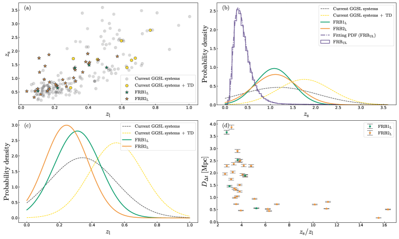
Figure 1: Simulated FRB data from a $5$-year CASM observation. Panel (a) shows the distributions of lens redshifts ($z_{\rm l}$) versus source redshifts ($z_{\rm s}$), with grey circles indicating current GGSL systems from Chen et al. (2019b) and yellow circles representing GGSL systems with TD measurements from Denzel et al. (2021). The green and orange stars denote simulated GGSL FRB data for scenarios with $5$ (normal) and $40$ (optimistic) sample sizes, labeled as $\rm FRB1_{\rm L}$ and $\rm FRB2_{\rm L}$, respectively, which are derived from the simulated sample of GGSL systems from Collett (2015). Note that $\rm FRB2_{\rm L}$ includes $\rm FRB1_{\rm L}$. Panels (b) and (c) display the normalized redshift distributions for $z_{\rm s}$ and $z_{\rm l}$, respectively. The lines of different colors and styles correspond to different datasets. The histogram of host galaxy redshift of unlensed FRBs ($\rm FRB_{\rm UL}$) is also illustrated in panel (b), with the normalized redshift distribution plotted as the purple line to show the lognormal+Cauchy fitting function (see Eq. (10)). Panel (d) illustrates the simulated TD distance data. Note that the fiducial model using the fiducial flat dynamical dark energy model with $w$ = constant.

Table 1: Uncertainties of three components contributing to the uncertainty of TD distance measurements. $\varepsilon(\Delta t)$, $\varepsilon(\Delta\psi)$, and $\varepsilon(\kappa_{\rm ext})$ correspond to the relative uncertainties of time delay, Fermat potential difference, and LOS contamination, respectively.

GGSL source	$\Delta t$	$\varepsilon(\Delta t)$	$\varepsilon(\Delta\psi)$	$\varepsilon(\kappa_{\rm ext})$
Lensed SNe	$\mathcal{O}(10^{6}~{}\rm s)$	3%	1%	3%
Lensed QSOs	$\mathcal{O}(\rm 1~{}s)$	5%	3%	3%
Lensed FRBs	$\mathcal{O}(10^{-6}~{}\rm s)$	0%	0.8%	2%

II.2 DM measurement from unlensed FRBs

We generate the DMs of unlensed FRB samples using the DM model in Ref. Zhang et al. (2023). The observed DM, $\rm DM_{\rm obs}$, is a measure of the number density of free electrons $n_{\rm e}$ weighted by $(1+z)^{-1}$, along the path $l$ to the FRB: ${\rm DM}_{{\rm obs}}=\int n_{{\rm e}}dl/(1+z)$. This value can be determined by the captive signal with the time delay between the highest frequency and the lowest frequency. Physically, $\rm DM_{\rm obs}$ is usually divided to four components: two from the Milky Way, i.e., one from the interstellar medium (ISM) and a second from its halo; and two extragalactic ones, the IGM and the FRB host galaxy,

$$\rm{DM}_{\rm{obs}}=\rm{DM}_{\rm{MW}}+\rm{DM}_{\rm{ext}}.$$ (6)

For the DM contribution within the Milky Way $\rm DM_{\rm MW}=\rm DM_{\rm MW,ISM}+\rm DM_{\rm MW,halo}$, $\rm DM_{\rm MW,ISM}$ can be obtained using the typical electron density models of the Milky Way, i.e., the NE2001 (Cordes and Lazio, 2002) and YMW16 (Yao et al., 2017) models. The calculation is related to the FRBs’ Galactic coordinates. $\rm DM_{\rm MW,halo}$ is in the range of [$30$, $80$]  pc cm^-3 (Dolag et al., 2015; Prochaska and Zheng, 2019a). In this study, we use the YMW16 model to calculate $\rm DM_{\rm MW,ISM}$ and assume a normal distribution to model $\rm DM_{\rm MW,halo}$ as $\mathrm{DM}_{\mathrm{MW,halo}}\sim\mathcal{N}(55,25^{2})$ (in units of  pc cm^-3 ) (Wu et al., 2022).

On the other hand, the extragalactic contribution, $\rm DM_{\rm ext}=\rm DM_{\rm IGM}+\rm DM_{\rm host}$, is typically the dominant part in $\rm DM_{\rm obs}$. $\rm{DM}_{\rm{IGM}}$ is closely related to cosmology, and the Macquart relation gives its averaged value (Macquart et al., 2020),

$$\langle{\rm DM}_{\rm IGM}(z)\rangle=\frac{3c\Omega_{\rm b}H_{0}}{8\pi Gm_{\rm p}}\int_{0}^{z}\frac{\chi(z^{\prime})f_{\rm{IGM}}(z^{\prime})(1+z^{\prime})}{E(z^{\prime})}dz^{\prime},$$ (7)

where $G$ is the gravitational constant, $m_{\rm{p}}$ is the mass of a proton, and $\chi(z)$ represents the number of free electrons per baryon, i.e., $\chi_{e}(z)=\frac{3}{4}\chi_{e,\rm{H}}(z)+\frac{1}{8}\chi_{e,\rm{He}}(z)$, where $\chi_{e,\rm{H}}$ and $\chi_{e,\rm{He}}$ are ionization fractions for hydrogen and helium, respectively. We take $\chi_{\rm{e,H}}=\chi_{\rm{e,He}}=1$, assuming that both hydrogen and helium are fully ionized at $z<3$. $f_{\rm{IGM}}(z)$ is the baryon fraction in the diffuse IGM evolving with redshift. It is suggested that $f_{\rm{IGM}}\simeq 0.9$ at $z\geq 1.5$ (Meiksin, 2009) and $f_{\rm{IGM}}\simeq 0.82$ at $z\leq 0.4$ (Shull et al., 2012) (see Refs. (Li et al., 2019; Wei et al., 2019; Li et al., 2020; Dai and Xia, 2021; Wang and Wei, 2023; Lin and Zou, 2023; Lemos et al., 2023) for other studies constraining $f_{\rm IGM}$). We adopt a moderate value of $f_{\rm{IGM}}\simeq 0.83$ for the redshift range considered in our sample. More importantly, $E(z)$, the dimensionless Hubble parameter, is directly related to cosmological parameters, which will be discussed further in sect. II.5.

Due to large fluctuations in the IGM, the actual value of $\rm DM_{\rm IGM}$ varies significantly around the mean value $\langle{\rm{DM}}_{{{\rm{IGM}}}}(z)\rangle$. The variation is mainly attributed to the galactic feedback (Walters et al., 2018). The probability distribution function (PDF) of $\rm DM_{\rm IGM}$ has been derived from numerical simulations of the IGM (McQuinn, 2013) and galaxy halos (Prochaska and Zheng, 2019b). Based on cosmological principles, the impact of compact halo contribution on large scales is insignificant, and we assume that the distribution of $\rm DM_{\rm IGM}$ follows a Gaussian distribution, with $\sigma_{\rm IGM}$ scaling with redshift in a power-law form as:

$$\sigma_{\rm{IGM}}(z)=Az^{\alpha}~{}\rm{pc}~{}\rm{cm}^{-3},$$ (8)

where $A$ is fitted to $173.8$, and $\alpha$ is $0.4$ (Qiang and Wei, 2021).

The contribution from host galaxy, $\rm DM_{\rm host}$, is difficult for modeling due to its strong dependence on the type of galaxy and local environment. Macquart et al. (2020) proposed a lognormal PDF with an asymmetric long tail allowing for high $\rm DM_{\rm host}$ values (e.g., that of FRB 20190520B (Niu et al., 2022)), which fits well with the results from the IllustrisTNG simulation (Zhang et al., 2020a). However, recent simulations suggest that $\rm DM_{\rm host}$ may deviate from this distribution (Beniamini et al., 2021; Orr et al., 2024). So the real distribution remains uncertain, which needs for larger FRB samples in future studies. We adopt a simplified physical scenario, assuming that the distribution of $\rm DM_{\rm host}$ also follows a Gaussian distribution with a standard deviation of $\sigma_{\rm{host}}=30~{}{\rm{pc~{}cm^{-3}}}$ (Li et al., 2019), which is expected to be realized in the high-statistics era.

Overall, $\rm{DM}_{\rm{IGM}}$ is available for a localized FRB with $\rm{DM}_{\rm{obs}}$, $\rm{DM}_{\rm{MW}}$ and $\rm{DM}_{\rm{host}}$ determined. The observational uncertainty is negligible compared to other errors and can be ignored. Consequently, if these parameters are treated properly, the total uncertainty of $\rm{DM}_{\rm{IGM}}$ is determined by

$$\sigma_{\rm{DM}_{\rm{IGM}}}=\left[\sigma_{\rm MW}^{2}+\sigma_{\rm IGM}^{2}+\left(\frac{\sigma_{\rm host}}{1+z}\right)^{2}\right]^{1/2},$$ (9)

where the uncertainty of $\rm{DM}_{\rm{MW}}$, i.e., $\sigma_{\rm MW}$, averages about $10~{}{\rm{pc~{}cm^{-3}}}$ for the pulses from high Galactic latitude $\left(|b|>10^{\circ}\right)$. The factor $(1+z)$ accounts for cosmological time dilation for a source at redshift $z$.

For the redshift distribution of the mock unlensed FRB data, we have fitted the distribution in Connor and Ravi (2023) with a lognormal$+$Cauchy PDF,

$$N(z)=\frac{1}{\sqrt{2\pi}\sigma z}\exp\left[-\frac{\left(\lg z-\mu\right)^{2}}{2\sigma^{2}}\right]+\frac{\gamma}{\pi((x-x_{0})^{2}+1)},$$ (10)

where parameters $\sigma$, $\mu$, $\gamma$, and $x_{0}$ are fitted to $0.45$, $-0.02$, $0.05$, and $1.60$, respectively. This is the assumed redshift distribution for the CASM, which is derived by scaling the redshift distribution from the latest CHIME catalog (Amiri et al., 2021).

II.3 Simulation of TD and DM measurements from CASM’s FRBs

Table 2: Main properties of CHIME, BURSTT-256, and CASM assumed in this work, corresponding to current, upcoming, and future-concept FRB observatories.

Specification	CHIME (Bandura et al., 2014)	BURSTT-256 (Lin et al., 2022)	CASM (Connor and Ravi, 2023)
Number of antennas	$1,024$	$256$	$\sim 25,000$
Frequency range (MHz)	$400$–$800$	$300$–$800$	$400$–$800$
Effective area ($\rm m^{2}$)	$8,000$	$40$–$200$	$8,000$
FoV ($\rm deg^{2}$)	$\sim 200$	10,000	5,000
SEFD (Jy)	$50$	$\sim 5,000$	$50$
Localization accuracy (′′)	$\sim 60$	$\sim 1$	$\sim 1$
Detection event rate ($\rm year^{-1}$)	$500$–$1,000$	$\sim 100$	$7,500$–$25,000$

We briefly introduce the CASM survey and then the simulation of both the TD distance and DM measurements from lensed FRBs.

So far, no gravitational lensing has been firmly identified in FRB signals (nevertheless, FRB 20190308C was recently reported as a plausible candidate with a significance of $3.4\sigma$ and requires further investigation (Chang et al., 2024)). This is likely due to missed detections, lensing below telescope sensitivity, or simply not being lensed within the observation period. To settle these issues, continuous coverage of a significant fraction of the sky may be the optimal way of finding strongly lensed FRBs (Wucknitz et al., 2021). The CASM facility can observe a unique all-sky collecting area, which will play a critical role in the blind FRB search. This is because surveys of transient events like FRBs benefit from a large FoV, as the number of detections increase proportionally with the FoV, while detecting persistent source depends on sensitivity, which increases with the square root of the FoV (Luo et al., 2024). An explicit example of CASM is the upcoming Bustling Universe Radio Survey Telescope for Taiwan (BURSTT) (Lin et al., 2022) project. BURSTT is the first telescope dedicated for a complete census of nearby FRBs with a long time window, which allows for monitoring of FRBs for repetition and counterpart identification. These would be clues to understanding the origins of FRBs, and there have been many efforts for answering whether all FRBs repeat (Chen et al., 2021; Luo et al., 2022; Zhu-Ge et al., 2022; Kirsten et al., 2024; Sun et al., 2024) and what their counterparts are (Andersen et al., 2020; Bochenek et al., 2020; Lin et al., 2020; Li et al., 2021b; Abbott et al., 2023; Moroianu et al., 2023; Qi-lin et al., 2024).

Due to its unique fisheye design, BURSTT has a extremely large instantaneous FoV of $\sim 10,000~{}\rm deg^{2}$, which is 25 times larger than that of CHIME. With VLBI outrigger stations, BURSTT can achieve a sub-acrsecond localization for identifying the unambiguous host galaxy. More importantly, BURSTT has been considered to search for lensed FRBs with short time delay (less than $\sim$ milliseconds) (Ho et al., 2023). Meanwhile, its wide FoV enables long-term, high-cadence monitoring of a large sky area, which can technically detect lensing delays up to the survey duration, and avoids missing potentially lensed FRBs with long time delays ($\sim$ days to months). This suggests that CASM experiments are particularly superior in detecting strongly lensed FRBs.

However, BURSTT is initially designed to detect hundreds of bright and nearby FRBs at $z\sim 0.03$ per year. To detect strongly lensed FRBs usually at higher redshifts, a high sensitivity is required for blind searches, which can be achieved by using a dense aperture array with substantial small antennas. BURSTT is built with 256 antennas (BURSTT-256) and is planned to expand to 2048 antennas (BURSTT-2048). The SEFD of BURSTT-256 is $\sim 600$ Jy, and that of BURSTT-2048 is $\sim$ 5,000 Jy, but both are still lower than CHIME’s SEFD of $50$ Jy. In principle, methods to improve sensitivity include reducing system temperature, increasing the number of antennas, and utilizing a compact phased array technology for beamforming (Luo et al., 2024). If the sensitivity matches that of CHIME, the number of detected FRBs would dramatically increase. Connor and Ravi (2023) assumed a future CASM survey with a large FoV of $\sim 5,000~{}\rm deg^{2}$ and an SEFD of $50$ Jy observing in the $400$–$800$ MHz band, which is equivalent to a CHIME/FRB survey but with $25$ times of the sky coverage. They predicted that such a survey could potentially detect 50,000–100,000 FRBs including $5$–$40$ lensed events, during a 5-year observation with an $80\%$ duty cycle (see Table 2 in Ref. Connor and Ravi (2023)). This estimation is purely based on the fact that the event rate is $25$ times larger than CHIME, without additional assumptions. If these FRBs can be well localized, they would be valuable for studying FRB cosmology, which requires a large sample of localized FRBs as well as potential lensed events. This is also what future BURSTT science pursues, focusing on key topics in cosmology and fundamental physics. We assumed that the CASM can also localize FRBs to the sub-acrsecond resolution like BURSTT, so the redshifts of the detected FRBs can be measured. The main properties of the CASM are summarized in the last column of Table 2, together with CHIME and BURSTT-256 for comparison.

In this work, we simulate the FRB data observed by the CASM survey (with a CHIME/FRB SEFD), using the methods for simulating TD measurement in sect. II.1 and DM measurement in sect. II.2. Based on the event rate estimation in Connor and Ravi (2023), we consider two scenarios: a conservative scenario with $5$ lensed FRBs (labeled as $\rm FRB1_{\rm L}$) and an optimistic scenario with $40$ lensed FRBs (labeled as $\rm FRB2_{\rm L}$), both within a sample of 100,000 unlensed FRBs (labeled as $\rm FRB_{\rm UL}$). Note that we focus on what role the lensed bursts can play in large samples, so for convenience, we assume the total detection of 100,000 FRBs. The mock lensed FRB data, which are derived from the mock strong lens sample in Collett (2015), are shown in Figure 1. In addition, the histogram of simulated unlensed FRBs and the fitting PDF (see Eq. (10)) are illustrated in purple in Figure 1(b). The redshift distributions of the mock lensed FRBs are consistent with that of the unlensed FRBs and significantly overlap with both the currently detected GGSL systems from Chen et al. (2019b) and those with TD measurements from Denzel et al. (2021).

II.4 Other cosmological data

Table 3: Absolute ($1\sigma$) and relative errors on cosmological parameters of interest in the $w$CDM and $w_{0}w_{a}$CDM models using the single dataset from early- or late-universe observation, i.e., CMB, $\rm FRB_{\rm UL}$, $\rm FRB1_{\rm L}$, and $\rm FRB2_{\rm L}$. Note that the mock FRB data are derived from a 5-year observation of BURSTT, including $\rm FRB_{\rm UL}$ with an unlensed event number of 100,000, as well as $\rm FRB1_{\rm L}$ and $\rm FRB2_{\rm L}$ with lensed event numbers of $5$ and $40$, respectively. Here, $H_{0}$ is in units of km s^-1 Mpc^-1.

        Model         Error         CMB         $\rm FRB_{\rm UL}$         $\rm FRB1_{\rm L}$         $\rm FRB2_{\rm L}$         $w$CDM         $\sigma(H_{0})$         6.20         —         1.35         0.52         $\varepsilon(H_{0})$         $9.0\%$         —         $2.0\%$         $0.8\%$         $\sigma(w)$         0.200         0.052         —         0.245         $\varepsilon(w)$         $19.2\%$         $5.1\%$         —         $19.6\%$         $w_{0}w_{a}$CDM         $\sigma(H_{0})$         7.60         —         1.65         0.70         $\varepsilon(H_{0})$         $11.0\%$         —         $2.4\%$         $1.0\%$         $\sigma(w_{0})$         0.450         0.105         —         0.835         $\varepsilon(w_{0})$         $54.0\%$         $11.0\%$         —         $68.0\%$         $\sigma(w_{a})$         —         0.85         —         1.65

In addition to mock FRB data, we incorporate complementary cosmological datasets, including the acutal CMB, BAO and SNe data, as well as mock GW datasets.

For the mock data, we employ the GW standard siren data from Ref. Zhang et al. (2023), which is generated based on the third-generation ground-based GW detector, the Einstein Telescope (ET) (Punturo et al., 2010). The GW standard siren method (Schutz, 1986; Holz and Hughes, 2005) is an emerging probe of the late universe, which gives $\sim 14\%$ precision in measuring $H_{0}$ through the only multi-messenger observations of GW170817 (Abbott et al., 2017). Recently, this method have widely informed forecasts of the cosmological parameter estimations based on the future standard sirens detected by ground-based (Zhao et al., 2011; Chen et al., 2018; Du et al., 2019; Chang et al., 2019; Zhang et al., 2020b; Jin et al., 2020, 2021; Cao et al., 2022; Wang et al., 2022b; Jin et al., 2022, 2023; Li et al., 2024b; Han et al., 2024; Jin et al., 2024a; Feng et al., 2024a; Dong et al., 2024; Zheng et al., 2024; Fu and Zhang, 2024; Feng et al., 2024b), space-borne (Cutler and Holz, 2009; Cai et al., 2018; Wang et al., 2020b; Zhao et al., 2020b; Wang et al., 2022c; Guo, 2022; Song et al., 2024; Jin et al., 2024b) GW observatories, and pulsar timing arrays projects (Yan et al., 2019; Wang et al., 2022d; Xiao et al., 2024b). These efforts detect GWs across various frequency bands from nanohertz to several hundred hertz (see Refs. Cai et al. (2017); Zhang (2019); Bian et al. (2021) for reviews). The absolute distance to a GW source can be determined by analyzing the GW waveform, where the amplitude in frequency domain is approximately inversely proportional to the luminosity distance $D_{\rm{L}}$. We consider only the binary neutron star (BNS) merger events, which could provide electromagnetic (EM) counterparts carrying redshift information. Then the established $D_{\rm{L}}$–$z$ relation can be used to study cosmology as

$$D_{\rm{L}}(z)=(1+z)\int_{0}^{z}\frac{dz^{\prime}}{H(z^{\prime})},$$ (11)

which is referred to as bright sirens. We only consider bright siren data in this work. The error in the measurement of $D_{\rm L}$ is calculated as

$$\sigma_{D_{\rm L}}=\left[(\sigma_{D_{\rm L}}^{\rm inst})^{2}+(\sigma_{D_{\rm L}}^{\rm lens})^{2}+(\sigma_{D_{\rm L}}^{\rm pv})^{2}\right]^{1/2},$$ (12)

where $\sigma_{D_{\rm L}}^{\rm inst}$, $\sigma_{D_{\rm L}}^{\rm lens}$, and $\sigma_{D_{\rm L}}^{\rm pv}$ are the instrumental, weak lensing, and peculiar velocity errors derived from Refs. (Nishizawa et al., 2011), (Hirata et al., 2010), and (Gordon et al., 2007), respectively. The ET is anticipated to detect $1,000$ bright sirens from BNS mergers at $z\lesssim 5$ during a 10-year observation period (Zhang et al., 2019). For more details on this simulation, readers can refer to Ref. Zhang et al. (2023).

In addition to mock data, we also utilize actual mainstream cosmological data, including the CMB, BAO, and SNe data. For the CMB data, we employ the “Planck distance priors” from the Planck 2018 observation Chen et al. (2019b), and we use the BAO measurements from 6dFGS at $z_{\rm eff}=0.106$ Beutler et al. (2011), SDSS-MGS at $z_{\rm eff}=0.15$ Ross et al. (2015), and Data Release $12$ of Baryon Oscillation Spectroscopic Survey (BOSS-DR12) at $z_{\rm eff}=0.38$, $0.51$, and $0.61$ Alam et al. (2017). For the SNe data, we use the sample from the Pantheon compilation with $1048$ supernovae data Scolnic et al. (2018).

We use the data combination CMB+BAO+SNe (abbreviated as “CBS”) to constrain the fiducial cosmological models, and the obtained best-fit cosmological parameters are used to generate the central values of DMs and TDs in the simulated FRB data.

II.5 Cosmological parameter estimation

We provide a overview of the adopted dark energy models and methods for cosmological parameter estimation.

The dark energy models considered in this work include flat $\Lambda$CDM, $w$CDM, and $w_{0}w_{a}$CDM models. The EoS parameter for dark energy, $w(z)$, is defined as the ratio of its pressure $p_{\rm{de}}(z)$ to density $\rho_{\rm{de}}(z)$ at redshift $z$. It helps describe the dimensionless Hubble parameter $E(z)$, which can be formulated using the Friedmann equation for a given cosmological model. In a spatially-flat universe, the dimensionless Hubble parameter $E(z)=H(z)/H_{0}$ is expressed as

$$E^{2}(z)=\Omega_{\rm m}(1+z)^{3}+(1-\Omega_{\rm m})\exp\left[3\int_{0}^{z}\frac{1+w(z^{\prime})}{1+z^{\prime}}dz^{\prime}\right],$$ (13)

where $\Omega_{\rm m}$ represents the present-day matter density parameter.

The simplest and most widely accepted dark energy model is the $\Lambda$CDM model with the vacuum energy EoS $w=-1$. The $w$CDM model, on the other hand, assumes a constant EoS $w$, representing the simplest scenario for dynamical dark energy. Finally, the $w_{0}w_{a}$CDM model describes an evolving EoS as $w(z)=w_{0}+w_{a}/(1+z)$, where $w_{0}$ and $w_{a}$ are the two parameters that characterize the evolution.

The cosmological parameters $\bm{\xi}$ we sample include $\Omega_{\rm m}$, $\Omega_{\rm b}h^{2}$, $w$, $w_{0}$, $w_{a}$, and $H_{0}$, and we take flat priors within ranges of $[0,1]$, $[0,0.05]$, $[-2,1]$, $[-5,1]$, $[-3,3]$, and $[0,100]$ $\rm km\ s^{-1}\ Mpc^{-1}$, respectively. They are optimized via maximization of the joint likelihood function,

$$\mathcal{L}\propto e^{-\chi^{2}/2},$$ (14)

where the $\chi^{2}$ function for lensed FRBs, unlensed FRBs, and GWs are defined as

$$\chi_{\mathrm{TD}}^{2}(\bm{\xi})=\sum_{i=1}^{N_{\rm FRB_{\rm L}}}\left(\frac{D_{\Delta t,i}^{\mathrm{th}}(\bm{\xi})-D_{\Delta t,i}^{\mathrm{obs}}}{\sigma_{D_{\Delta t}}(z_{i})}\right)^{2},$$ (15)

$$\chi_{\rm DM}^{2}(\bm{\xi})=\sum_{i=1}^{N_{\rm FRB_{\rm UL}}}\left(\frac{{\rm{DM}_{\rm{IGM}}^{\rm{th}}}(z_{i};{\bm{\xi}})-{\rm{DM}_{\rm{IGM}}^{\rm{obs}}}(z_{i})}{\sigma_{\rm{DM}_{\rm{IGM}}}(z_{i})}\right)^{2},$$ (16)

and

$$\chi_{\rm{GW}}^{2}(\bm{\xi})=\sum_{i=1}^{N_{\rm GW}}\left(\frac{D_{\rm{L}}^{\rm{th}}(z_{i};{\bm{\xi}})-D_{\rm{L}}^{\rm{obs}}(z_{i})}{\sigma_{D_{\rm L}}(z_{i})}\right)^{2},$$ (17)

respectively. $D_{\Delta t}^{\mathrm{obs}}$, $\rm{DM}_{\rm{IGM}}^{\rm{obs}}$, and $D_{\rm{L}}^{\rm{obs}}$ are the observable values, and $D_{\Delta t,i}^{\mathrm{th}}(\bm{\xi})$, ${\rm DM}_{\rm{IGM}}^{\rm{th}}(z_{i};\bm{\xi})$, and $D_{\rm{L}}^{\rm{th}}(z_{i};{\bm{\xi}})$ are theoretical values of $D_{\Delta t}$, $\rm{DM}_{\rm{IGM}}$ and $D_{\rm{L}}$ at $z_{i}$ calculated by Eqs. (4), (7), and (11), respectively. $\sigma_{D_{\Delta t}}(z_{i})$, $\sigma_{\rm{DM}_{\rm{IGM}}}$($z_{i}$), and $\sigma_{d_{\rm L}}(z_{i})$ represent the related uncertainties calculated by Eqs. (5), (9), and (12).

We derive the posterior probability distributions through the Markov chain Monte Carlo analysis (MCMC) ensemble sampler emcee (Foreman-Mackey et al., 2013), and use GetDist for plotting the posterior distributions of the cosmological parameters.

III Results and discussion

Table 4: Same as Table 3 but using the combined datasets from both early- and late-universe observations, i.e., CBS, CMB+$\rm FRB_{\rm UL}$, CMB+$\rm FRB1_{\rm L}$, and CMB+$\rm FRB2_{\rm L}$ data. Here, CBS stands for CMB+BAO+SNe and $H_{0}$ is in units of km s^-1 Mpc^-1.

      Model       Error       CBS       CMB+$\rm FRB_{\rm UL}$       CMB+$\rm FRB1_{\rm L}$       CMB+$\rm FRB2_{\rm L}$       $w$CDM       $\sigma(H_{0})$       0.83       0.35       0.79       0.28       $\varepsilon(H_{0})$       $1.2\%$       $0.5\%$       $1.2\%$       $0.4\%$       $\sigma(w)$       0.034       0.019       0.036       0.026       $\varepsilon(w)$       $3.4\%$       $1.9\%$       $3.5\%$       $2.6\%$       $w_{0}w_{a}$CDM       $\sigma(H_{0})$       0.84       0.48       1.50       0.55       $\varepsilon(H_{0})$       $1.2\%$       $0.7\%$       $2.2\%$       $0.8\%$       $\sigma(w_{0})$       0.084       0.068       0.280       0.110       $\varepsilon(w_{0})$       $8.5\%$       $6.8\%$       $30.4\%$       $11.1\%$       $\sigma(w_{a})$       0.32       0.21       0.90       0.35

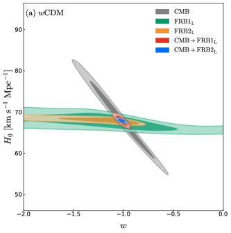
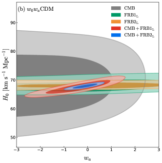
Figure 2: Two-dimensional posterior distribution ($68.3\%$ and $95.4\%$ credible regions) in the $w$–$H_{0}$ plane for the $w$CDM model (a) and the $w_{a}$–$H_{0}$ plane for the $w_{0}w_{a}$CDM model (b), by using the CMB, CBS, FRB$1_{\rm L}$, CMB+FRB$1_{\rm L}$, and CMB+FRB$2_{\rm L}$ data. Here, CBS stands for CMB+BAO+SNe.

In this section, we employ the simulated FRB observation from CASM to constrain two dynamical dark energy models, i.e., $w$CDM and $w_{0}w_{a}$CDM models. For comparison and combination, we also use the actual CMB, BAO, and SNe data, as well as the simulated GW data. The constraint results for key cosmological parameters, i.e., $H_{0}$ and the EoS of dark energy, are summarized in Tables 3–6 and shown in Figures 2–7 using different datasets. Here, we use $\sigma(\xi)$ and $\varepsilon(\xi)=\sigma(\xi)/\xi$ to represent the absolute and relative errors of the parameter $\xi$, respectively.

In the following, we first report the results separately from unlensed FRBs and lensed events in sect. III.1, and their joint analyses with CMB in sect. III.2. Then we present the results from combining the lensed and the unlensed FRBs into a full sample in sect. III.3. Finally, we discuss the combination of this full FRB dataset with CBS in sect. III.4.

III.1 The lensed or unlensed FRB data

We first report the constraint results from the FRB dataset of either unlensed or lensed events, i.e., $\rm FRB_{\rm UL}$, $\rm FRB1_{\rm L}$, and $\rm FRB2_{\rm L}$ in Tables 3, which represent a single probe from the late-universe observation.

When considering dynamical dark energy, the CMB data alone cannot give precise constraints, with $\varepsilon(H_{0})=9.0\%$ and $\varepsilon(w)=19.2\%$ in the $w$CDM model. In contrast, the FRB datasets can provide more precise constraints. A large number of 100,000 FRB data can effectively constrain dark-energy EoS parameters. Concretely, $\rm FRB_{\rm UL}$ gives an absolute error of $\sigma(w)=0.052$ in the $w$CDM model, and $\sigma(w_{0})=0.053$ and $\sigma(w_{a})=0.85$ in the $w_{0}w_{a}$CDM model. The constraints are all about $74\%$ better than those from the actual CMB data. However, it cannot constrain $H_{0}$ due to the strong parameter degeneracy between $\Omega_{\rm b}h^{2}$ and $H_{0}$ in Eq. (7).

On the other hand, if the lensed events are detected, they will provide very precise measurement on $H_{0}$. We give some examples in the $w_{0}w_{a}$CDM model. By using $5$ and $40$ lensed FRB data, FRB$1_{\rm L}$ and FRB$2_{\rm L}$ offer $H_{0}$ constraints with $2.4\%$ and $1.0\%$ precision, respectively, which are about $78\%$ and $92\%$ more precise than that of the CMB data, respectively. Nevertheless, using the lensed data is insufficient to effectively constrain dark energy, with the most precise constraint of $\sigma(w)=0.245$.

Overall, the future FRB observation with CASM can effectively measure dark energy and the Hubble constant, by analyzing DM and TD measurements from localized FRB datasets, respectively.

III.2 Combination with the CMB data

Figure 3: Two-dimensional posterior distribution ($68.3\%$ and $95.4\%$ credible regions) in the $w$–$H_{0}$ plane for the $w$CDM model, by using the CBS, CMB+FRB_UL, CMB+FRB$1_{\rm L}$, and CMB+FRB$2_{\rm L}$ data.

Next, we report the results from combining the CMB data with FRB datasets of either unlensed or lensed events, i.e., CMB+$\rm FRB_{\rm UL}$, CMB+$\rm FRB1_{\rm L}$, and CMB+$\rm FRB2_{\rm L}$ in Tables 4, which represent multiple probes from both early- and late-universe observations. We mainly discuss the results from the combined case of the lensed FRBs.

Current mainstream low-redshift observations, BAO and SNe, cannot independently constrain dark energy but can effectively break parameter degeneracies inherent in the CMB. By combining CMB with BAO+SNe, the CBS data offers greatly improved constraints: $\varepsilon(H_{0})=1.2\%$ and $\varepsilon(w)=3.4\%$.

Similarly, we find that when combining the CMB data, the lensed FRB data can precisely constrain both $H_{0}$ and dark-energy EoS parameters. The combination greatly improves the constraints over either single probe. We give some examples in the $w$CDM model. When compared to the CMB data alone, CMB+FRB$1_{\rm L}$ provides constraints in precision of $\varepsilon(H_{0})=1.2\%$ and $\varepsilon(w)=3.5\%$, which are improved by about $87\%$ and $82\%$, respectively. Also, when compared to the FRB$1_{\rm L}$ and FRB$2_{\rm L}$ data alone, CMB+FRB$1_{\rm L}$ and CMB+FRB$2_{\rm L}$ improve the constraints on $H_{0}$ by about $40\%$ and $50\%$, respectively. It is noteworthy that the lensed FRBs can effectively probe dark energy with the help of CMB. Figures 2(a) and 2(b) show the posterior contours in the $w$–$H_{0}$ and $w_{a}$–$H_{0}$ planes, respetively, by using the CMB, CBS, FRB$1_{\rm L}$, FRB$2_{\rm L}$, CMB+FRB$1_{\rm L}$, and CMB+FRB$2_{\rm L}$ data. The results indicate that the lensed FRB data can well break the parameter degeneracy induced by CMB.

To assess the extent of this capability, we make some comparative analyses. Previous studies Liu et al. (2019); Zhao et al. (2020a); Qiu et al. (2022); Zhao et al. (2023) demonstrated that combining CMB with FRB data can effectively improve cosmological constraints. Accordingly, we include the constraint contours of both CBS and CMB+$\rm FRB_{\rm UL}$ in Figure 3 for comparison with those of CMB+FRB$1_{\rm L}$ and CMB+FRB$2_{\rm L}$ for the $w$CDM model.

When compared to CBS, we can see that CMB+FRB$1_{\rm L}$ gives similar constraints on both $H_{0}$ and $w$, and CMB+FRB$2_{\rm L}$ provides even tighter measurements for these parameters. Note that for the $w_{0}w_{a}$CDM model, CMB+FRB$2_{\rm L}$ also offers constraints similar to CBS, with a better precision of $\varepsilon(H_{0})=0.8\%$, and slightly less precise results of $\varepsilon(w_{0})=11.1\%$ and $\sigma(w_{a})=0.35$. These suggest that using $5$–$40$ lensed FRBs alone can effectively break the inherent parameter degeneracies in CMB, comparable to using the combination of BAO+SNe.

On the other hand, when compared to CMB+$\rm FRB_{\rm UL}$, the constraints on $H_{0}$ from CMB+FRB$2_{\rm L}$ are more precise than those from CMB+$\rm FRB_{\rm UL}$ in Figure 3. Specifically, CMB+FRB$2_{\rm L}$ achieves $20\%$ better precision of $\varepsilon(H_{0})=0.4\%$, and slightly worse precision of $\varepsilon(w)=2.6\%$ than CMB+FRB_UL (giving $\varepsilon(H_{0})=0.5\%$ and $\varepsilon(w)=1.9\%$). They give similar constraint results.

Overall, we conclude that the effect of only $5$ lensed FRBs could be similar to that of BAO+SNe in breaking the CMB degeneracies, and $40$ lensed FRBs could even be comparable to 100,000 unlensed FRBs.

III.3 The joint lensed and unlensed FRB data

Table 5: Same as Table 3 but using the combined datasets from late-universe observations alone, i.e., FRB+BAO+SNe, FRB+GW, $\rm FRB_{\rm UL}+FRB1_{\rm L}$, and $\rm FRB_{\rm UL}+FRB2_{\rm L}$ data. Note that the mock GW data are derived from a 10-year observation of ET, with an expected event number of 1,000. Here, $H_{0}$ is in units of km s^-1 Mpc^-1.

Model Error $\rm FRB_{\rm UL}$+BAO+SNe $\rm FRB_{\rm UL}$+GW $\rm FRB_{\rm UL}$+$\rm FRB1_{\rm L}$ $\rm FRB_{\rm UL}$+$\rm FRB2_{\rm L}$ $w$CDM $\sigma(H_{0})$ 2.50 0.42 0.71 0.30 $\varepsilon(H_{0})$ $1.2\%$ $0.6\%$ $1.0\%$ $0.4\%$ $\sigma(w)$ 0.045 0.049 0.051 0.046 $\varepsilon(w)$ $4.4\%$ $4.8\%$ $5.0\%$ $4.5\%$ $w_{0}w_{a}$CDM $\sigma(H_{0})$ 4.15 0.80 0.89 0.51 $\varepsilon(H_{0})$ $6.1\%$ $1.2\%$ $1.3\%$ $0.7\%$ $\sigma(w_{0})$ 0.068 0.095 0.096 0.072 $\varepsilon(w_{0})$ $6.9\%$ $9.8\%$ $9.9\%$ $7.4\%$ $\sigma(w_{a})$ 0.61 0.80 0.79 0.70

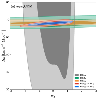
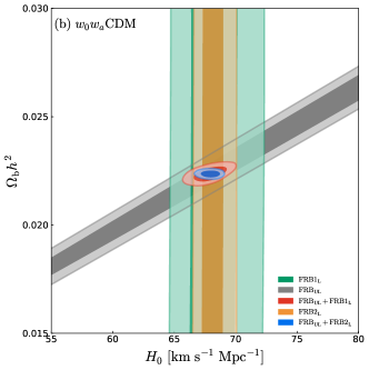
Figure 4: Two-dimensional posterior distribution ($68.3\%$ and $95.4\%$ credible regions) in the $w_{a}$–$H_{0}$ plane (a) and the $H_{0}$–$\Omega_{\rm b}h^{2}$ plane (b) for the $w_{0}w_{a}$CDM model, by using diferent FRB samples, i.e., the $\rm FRB_{\rm UL}$, FRB$1_{\rm L}$, $\rm FRB2_{\rm L}$, $\rm FRB_{\rm UL}$+FRB$1_{\rm L}$, and $\rm FRB_{\rm UL}$+FRB$2_{\rm L}$ data.

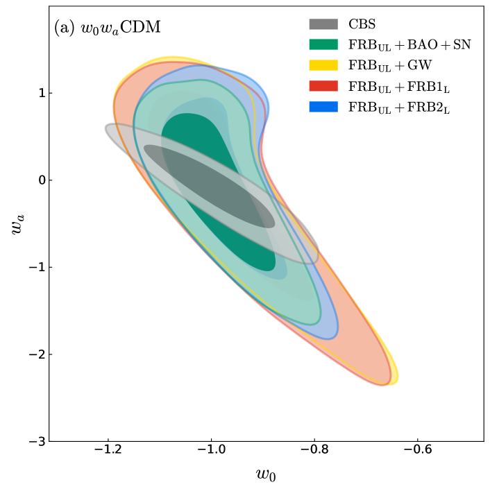
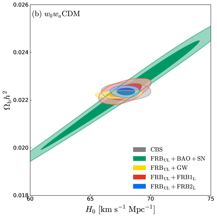
Figure 5: Two-dimensional posterior distribution ($68.3\%$ and $95.4\%$ credible regions) in the $w_{0}$–$w_{a}$ plane (a) and the $H_{0}$–$\Omega_{\rm b}h^{2}$ plane (b) for the $w_{0}w_{a}$CDM model, by using the CBS, $\rm FRB_{\rm UL}$+BAO+SNe, $\rm FRB_{\rm UL}$+GW, $\rm FRB_{\rm UL}$+$\rm FRB1_{\rm L}$, and $\rm FRB_{\rm UL}$+$\rm FRB2_{\rm L}$ data.

As the main focus of this paper, we report the constraint results from the full FRB dataset of both unlensed and lensed events, i.e., $\rm FRB_{\rm UL}$+$\rm FRB1_{\rm L}$ and $\rm FRB_{\rm UL}$+$\rm FRB2_{\rm L}$ in Table 5, which represent multiple probes from late-universe observations alone.

Here we emphasize two advantages of jointly analyzing the unlensed and lensed FRB data: (i) It serves as pure late-universe probes, thereby avoiding the impact of the tension between the early and late universe. (ii) It holds promise for precisely constraining key cosmological parameters, where unlensed and lensed FRBs can give tight constraints on dark energy and the Hubble constant, respectively, as shown in sect. III.1. In upcoming FRB observations, e.g., of CASM, a large detected FRB sample may harbor lensed bursts that have yet to be identified, so the joint method leads to an in-depth analysis that explores the cosmological value of the future FRB sample.

It is evident that the FRB sample with lensed events can simultaneously provide precise measurements of $H_{0}$ and the EoS of dark energy. Remarkably, the addition of the unlensed events to the lensed can significantly improve the constraint on $H_{0}$. For example, in the $w$CDM model, the combinations of $\rm FRB_{\rm UL}$+$\rm FRB1_{\rm L}$ and $\rm FRB_{\rm UL}$+$\rm FRB2_{\rm L}$ achieve precision of $\varepsilon(H_{0})=1.0\%$ and $\varepsilon(H_{0})=0.4\%$, respectively, which are improved by about $47\%$ and $42\%$ compared with using the $\rm FRB1_{\rm L}$ and $\rm FRB2_{\rm L}$ data alone, respectively. However, the joint analysis does not effectively improve the constraints on dark-energy EoS parameters compared to using the unlensed FRB data alone. Quantitatively, in the $w_{0}w_{a}$CDM model, the constraints on $w_{a}$ from $\rm FRB_{\rm UL}$+$\rm FRB1_{\rm L}$ and $\rm FRB_{\rm UL}$+$\rm FRB2_{\rm L}$ are only about $7\%$ and $17\%$ better, respectively, than those from $\rm FRB_{\rm UL}$ alone. Note that in the $w$CDM model, the improvements are even less significant. This is because the large number of unlensed FRBs already provide strong constraints on dark energy, weakening the contributions of additional probes. Figures 4(a) and 4(b) show the posterior contours in the $w_{a}$–$H_{0}$ and $H_{0}$–$\Omega_{\rm b}h^{2}$ planes, respectively, by using different FRB datasets. The different orientations of the contours constrained by $\rm FRB_{\rm UL}$ and lensed FRBs allow for mutually breaking parameter degeneracies. Obviously, the effect is more significant for the parameter $H_{0}$ than for $w_{a}$, leading to very different improvements in the joint analysis.

To explore the cosmological potential of combining lensed and unlensed FRBs, we compare the results with those from combining FRB datasets with low-redshift cosmological probes like BAO, SNe, and GW. The BAO+SNe combination represents current optical probes, while GW serves as a promising non-optical probe. Future GW bright standard sirens can precisely constrain the Hubble constant, but effective constraints on dark-energy EoS parameters require supports from additional external probes. Zhang et al. (2023) have found that the synergy between future GW and FRB observations can achieve sub-percent precision on $H_{0}$. Consequently, we have included the constraints from $\rm FRB_{\rm UL}$+BAO+SNe and $\rm FRB_{\rm UL}+GW$ in Table 4 for comparison. We also plot the two-dimensional constraint contours of CBS, $\rm FRB_{\rm UL}$+BAO+SNe, $\rm FRB_{\rm UL}$+GW for the $w_{0}w_{a}$CDM model in Figure 5, comparing them with contours from $\rm FRB_{\rm UL}$+FRB$1_{\rm L}$ and $\rm FRB_{\rm UL}$+FRB$2_{\rm L}$. We first report the constraints of dark energy, and then those of the Hubble constant.

For constraining dark energy, any of the above combinations cannot significantly improve the constraints. From Figure 5(a) showing the $w_{0}$–$w_{a}$ plane, we can see that the contours from $\rm FRB_{\rm UL}$+GW, $\rm FRB_{\rm UL}$+$\rm FRB1_{\rm L}$, $\rm FRB_{\rm UL}$+$\rm FRB2_{\rm L}$, $\rm FRB_{\rm UL}$+BAO+SNe, and CBS seem increasingly tighter. When combining unlensed and lensed FRBs, the constraints provided by $\rm FRB_{\rm UL}$+$\rm FRB1_{\rm L}$, with $\sigma(w_{0})=0.096$ and $\sigma(w_{a})=0.79$, are very similar to those from the $\rm FRB_{\rm UL}$+GW, with $\sigma(w_{0})=0.095$ and $\sigma(w_{a})=0.80$. Furthermore, $\rm FRB_{\rm UL}$+$\rm FRB2_{\rm L}$ offers slightly worse constraints than $\rm FRB_{\rm UL}$+BAO+SNe, with $\sigma(w_{0})=0.072$ and $\sigma(w_{a})=0.70$ for the former, versus $\sigma(w_{0})=0.068$ and $\sigma(w_{a})=0.61$ for the latter. It is worth noting that the constraint on $w_{0}$ from $\rm FRB_{\rm UL}$+$\rm FRB2_{\rm L}$ is $14\%$ more precise than that from CBS. We conclude that the inclusion of lensed FRBs in the unlensed sample could still deliver improvements of dark energy constraints, which is similar to including other late-universe probes: adding $5$ lensed FRBs is comparable to adding GW, and adding $40$ lensed FRBs is slightly weaker than adding BAO+SNe, but the $w_{0}$ constraint could still be better than that from CBS.

For constraining the Hubble constant, combining the lensed and unlensed FRBs can provide tighter constraints than other combinations. In the $H_{0}$–$\Omega_{\rm b}h^{2}$ plane, Figure 5(b) shows increasingly tighter contours from $\rm FRB_{\rm UL}$+BAO+SNe, $\rm FRB_{\rm UL}$+$\rm FRB1_{\rm L}$, CBS, $\rm FRB_{\rm UL}$+GW, and $\rm FRB_{\rm UL}$+$\rm FRB2_{\rm L}$. We give some examples in the $w_{0}w_{a}$CDM model. We find that $\rm FRB_{\rm UL}$+$\rm FRB1_{\rm L}$ gives $H_{0}$ constraints similar to CBS, with precision of $\varepsilon(H_{0})=1.3\%$, compared to $\varepsilon(H_{0})=1.2\%$ from CBS. Furthermore, $\rm FRB_{\rm UL}$+$\rm FRB2_{\rm L}$ delivers about a $36\%$ better constraint on $H_{0}$ compared to $\rm FRB_{\rm UL}$+GW. Specifically, $\rm FRB_{\rm UL}$+$\rm FRB2_{\rm L}$ gives $\varepsilon(H_{0})=0.7\%$, meeting the standard of precision cosmology, while $\rm FRB_{\rm UL}$+GW offers about $\varepsilon(H_{0})=1.2\%$. These results show that, including $5$ lensed events in a sample of 100,000 FRBs can constrain $H_{0}$ with the precision similar to CBS, and including $40$ lensed FRBs could exceed that of including $1,000$ standard siren data from the future GW observation of ET.

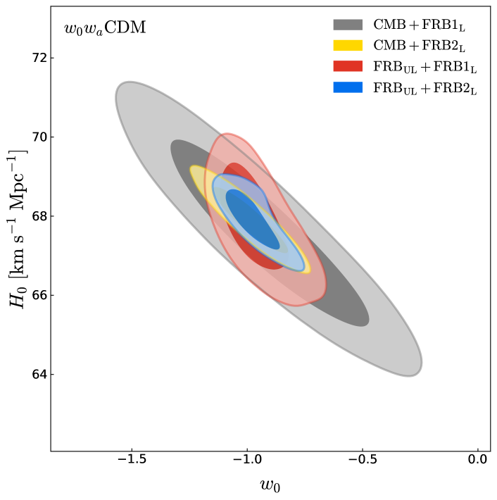
Figure 6: Two-dimensional posterior distribution ($68.3\%$ and $95.4\%$ credible regions) in the $w_{0}$–$H_{0}$ plane for the $w$CDM model, by using the CMB+FRB1_L, CMB+FRB2_L, $\rm FRB_{\rm UL}$+$\rm FRB1_{\rm L}$, and $\rm FRB_{\rm UL}$+$\rm FRB2_{\rm L}$ data.

Interestingly, we also compare the combined results of lensed FRBs with unlensed FRBs and CMB, and find that $\rm FRB_{\rm UL}$+$\rm FRB_{\rm L}$ could yield even more precise measurement of cosmological parameters than CMB+$\rm FRB_{\rm L}$ from Figure 6. For example, the constraints on $H_{0}$, $w_{0}$, and $w_{a}$ from $\rm FRB_{\rm UL}$+$\rm FRB1_{\rm L}$ are $\sim 40\%$, $67\%$, and $12\%$ more precise, respectively, than those from CMB+$\rm FRB1_{\rm L}$ for the $w_{0}w_{a}$CDM models. The constraints from combining both lensed and unlensed FRB data could be not only precise but also a late-universe result derived from the FRB observation alone. The dual advantages provide a potential cross-check against the “Hubble tension”.

Overall, we conclude that the joint analysis of unlensed and lensed FRB datasets of CASM is highly valuable, which can significantly improve the precision in measuring the Hubble constant. The effect of combining the lensed FRBs with the unlensed ones is better than combining the future GW observation (with the unlensed FRBs) , and combining the unlensed FRBs with the lensed ones could be more effective than combining the CMB observation (with the lensed FRBs).

Table 6: Same as Table 3 but using the the combined datasets from current and future cosmological observations, i.e., CBS+GW, CBS+$\rm FRB_{\rm UL}$+$\rm FRB1_{\rm L}$, and CBS+$\rm FRB_{\rm UL}$+$\rm FRB2_{\rm L}$ data. Here CBS stands for CMB+BAO+SNe. $H_{0}$ is in units of km s^-1 Mpc^-1.

Model	Error	CBS+GW	CBS+$\rm FRB_{\rm UL}$+$\rm FRB1_{\rm L}$	CBS+$\rm FRB_{\rm UL}$+$\rm FRB2_{\rm L}$
$w$CDM	$\sigma(H_{0})$	0.51	0.30	0.21
	$\varepsilon(H_{0})$	$0.8\%$	$0.4\%$	$0.3\%$
	$\sigma(w)$	0.028	0.017	0.017
	$\varepsilon(w)$	$2.8\%$	$1.7\%$	$1.7\%$
$w_{0}w_{a}$CDM	$\sigma(H_{0})$	0.62	0.38	0.29
	$\varepsilon(H_{0})$	$0.9\%$	$0.6\%$	$0.4\%$
	$\sigma(w_{0})$	0.067	0.051	0.046
	$\varepsilon(w_{0})$	$6.5\%$	$5.1\%$	$4.6\%$
	$\sigma(w_{a})$	0.22	0.16	0.15

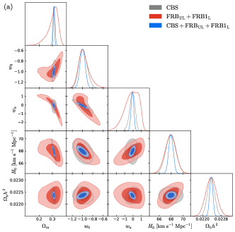
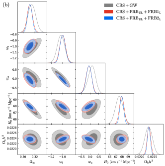
Figure 7: Three-dimensional posterior distribution ($68.3\%$ and $95.4\%$ credible regions) for the $w_{0}w_{a}$CDM model, by using the CBS, $\rm FRB_{\rm UL}$+$\rm FRB1_{\rm L}$, and CBS+$\rm FRB_{\rm UL}$+$\rm FRB1_{\rm L}$ data (a) and the CBS+GW, $\rm FRB_{\rm UL}$+$\rm FRB1_{\rm L}$, and CBS+$\rm FRB_{\rm UL}$+$\rm FRB2_{\rm L}$ data (b).

III.4 Combination with the CBS data

Finally, we report the constraint results from combining the CBS data with the full FRB dataset, i.e., CBS+FRB_UL+FRB1_L and CBS+FRB_UL+FRB2_L in Table 5, which represent multiple probes from current and future cosmological observations.

We find that with the addition of $\rm FRB_{\rm UL}$+FRB$1_{\rm L}$ to CBS, the constraint precisions of $w_{0}$ and $H_{0}$ are improved from $9.9\%$ and $1.2\%$ to $5.1\%$ and $0.6\%$, respectively. For the parameter $w_{a}$, the absolute constraint error is significantly improved from $0.79$ to $0.16$, with a significant increase in precision of about $80\%$. We plot three-dimensional posterior contours in Figure 7(a) for the $w_{0}w_{a}$CDM model. As can be seen, the improvements are also evident for the parameters $\Omega_{\rm m}$ and $\Omega_{\rm b}h^{2}$. Hence, the FRB observation of CASM will significantly improve current constraint precision of cosmological parameters.

To study the ability of the full FRB samples to improve cosmological parameter estimation, we compare the combinations CBS+$\rm FRB_{\rm UL}$+FRB_L with CBS+GW, which also represent multi-wavelength and multi-messenger observations, respectively. Meanwhile, we can thus investigate what precision the two perspectives of multiple probes may achieve in the future. Constraint contours of CBS+GW, CBS+$\rm FRB_{\rm UL}$+FRB$1_{\rm L}$, and CBS+$\rm FRB_{\rm UL}$+FRB$2_{\rm L}$ for the $w_{0}w_{a}$CDM model are shown in Figure 7(b). We can clearly see that the contours from the joint CBS+$\rm FRB_{\rm UL}$+$\rm FRB_{\rm L}$ data are both tighter than those from CBS+GW. For example, the constraints from CBS+$\rm FRB_{\rm UL}$+FRB$2_{\rm L}$ include $\sigma(H_{0})=0.29~{}{\rm km~{}s^{-1}~{}Mpc^{-1}}$, $\sigma(w_{0})=0.046$, and $\sigma(w_{a})=0.15$. For the concerned parameters $H_{0}$, $w_{0}$, and $w_{a}$, the absolute errors from CBS+$\rm FRB_{\rm UL}$+$\rm FRB_{\rm L}$ are smaller than those from CBS+GW by about $39\%$–$53\%$, $24\%$–$31\%$, and $27\%$–$32\%$, respectively.

Overall, we conclude that when combining current cosmological probes, the FRB detections of CASM may outperform the GW detections of ET in constraining cosmological parameters. This reinforces the cosmological implication of a multi-wavelength observational strategy in optical and radio bands.

IV Conclusion

In this paper, we forecast cosmological parameter estimation using localized FRBs from the future sensitive CASM survey. With continuous wide-field monitoring and high sensitivity, the CASM is expected to detect and localize a large sample of FRBs, which potentially include strongly lensed events by massive galaxies. The study of FRB cosmology will greatly benefit from precise TD measurement of lensed bursts and DM information of abundant unlensed ones, via the time-delay cosmography and the Macquart relation, respectively. We have employed both methods to study the cosmological potential of the simulated FRB sample with the CASM. By using MCMC techniques, we have mainly focused on the constraints on the Hubble constant and dark-energy EoS parameters within the fiducial flat dynamical dark energy framework (i.e., the flat $w$CDM and $w_{0}w_{a}$CDM models). Based on different datasets, we have the following main findings.

(i) Using only the FRB dataset of either unlensed or lensed events as an independent late-universe probe, we found that a large number of 100,000 FRBs can effectively constrain dark-energy EoS parameters, with constraint error of $\sigma(w)=0.052$ in the $w$CDM model, and using $5$ and $40$ lensed FRB data can measure the Hubble constant with relative errors of $\varepsilon(H_{0})=2.4\%$ and $\varepsilon(H_{0})=1.0\%$ in the $w_{0}w_{a}$CDM model, respectively.

(ii) Combining CMB with lensed FRBs as multiple probes from both early- and late-universe observations, we found that, the lensed FRB data can greatly improve the constraints over either single probe, by well breaking the parameter degeneracy induced by the CMB data. Compared to using the CMB and lensed FRB data alone, the joint analyses improve $H_{0}$ constraints by about over $80\%$ and $40\%$ for both $w$CDM and $w_{0}w_{a}$CDM models, respectively. The effect of only $5$ lensed FRBs could be similar to that of current BAO+SNe in breaking the CMB degeneracies, and $40$ lensed FRBs could even be comparable to 100,000 unlensed FRBs.

(iii) Using the full FRB dataset of both unlensed and lensed events as multiple late-universe probes enables an in-depth cosmological analysis of the localized FRB samples, avoiding the impact of the tension between the early and late universe. We found that the combination can simultaneously constrain the Hubble constant and dark energy, with high precision of $\varepsilon(H_{0})=0.4\%$ and $\varepsilon(w)=4.5\%$ in the $w$CDM model. The inclusion of the lensed events to the unlensed ones can significantly improve the $H_{0}$ constraint; for example, including $5$ lensed FRBs can achieve the precision similar to CBS, and including $40$ lensed FRBs could exceed that of including other emerging late-universe probe like $1,000$ GW standard sirens from future ET’s observation. Although the constraints on dark energy are not significantly improved, the joint analysis could still offer improvements comparable to those from combining the unlensed FRBs with BAO+SNe. Interestingly, the combination $\rm FRB_{\rm UL}$+$\rm FRB_{\rm L}$ could yield more precise constraints than CMB+$\rm FRB_{\rm L}$. Overall, the joint analysis of unlensed and lensed FRB datasets of the CASM is highly valuable, which can significantly improve the precision in measuring $H_{0}$. The synergy could be more effective than combining either the unlensed FRBs with future GW standard sirens or the lensed FRBs with CMB.

(iv) Combining CBS with the full FRB datasets as multiple probes from current and future cosmological observations, we found that the joint CBS and $\rm FRB_{\rm UL}$+$\rm FRB2_{\rm L}$ data give $\sigma(H_{0})=0.29~{}{\rm km~{}s^{-1}~{}Mpc^{-1}}$, $\sigma(w_{0})=0.046$, and $\sigma(w_{a})=0.15$ in the $w_{0}w_{a}$CDM model. The constraint results from the joint CBS+$\rm FRB_{\rm UL}$+FRB_L data are about $50\%$–$80\%$ tighter than those from CBS, and about $30\%$–$50\%$ than those from CBS+GW. Therefore, the FRB observation of the CASM will significantly improve current constraint precision of cosmological parameters, which may outperform the GW detections of ET in constraining cosmological parameters. This reinforces the cosmological implications of a multi-wavelength observational strategy in optical and radio bands.

This study aims to preliminarily explore the prospect of FRB cosmology, particularly considering the effect of strong gravitational lensing. It remains challenging to address the bias induced by systematic errors from the both two methods and large-scale structure (Reischke and Hagstotz, 2023; Takahashi, 2024), as well as to observationally determine the FRB redshift from its host (Jahns-Schindler et al., 2023; Marnoch et al., 2023). Nevertheless, future ambitious FRB observations are expected to resolve these issues and greatly contribute to deciphering the nature of dark energy, as well as resolving the Hubble tension if enough events with long-duration lensing are incorporated.