Numerical investigation of buoyancy-aided mixed convective flow past a square cylinder inclined at 45 degrees

Abstract

The present study numerically investigates two-dimensional mixed convective flow of air past a square cylinder placed at an angle of incidence of $\alpha=45^{\circ}$ to the free-stream. We perform direct numerical simulations (DNS) for a Reynolds number (Re) of 100 and a range of Richardson numbers (Ri) between 0.0 and 1.0 and a Prandtl number (Pr) of 0.7. The critical Richardson number at which the near-field becomes a steady flow from an unsteady one, using Stuart-Landau analysis, is found to be Ri $=0.68$, and simultaneously, the far-field unsteadiness emerges. There is no range of Ri for which the entire flow field is seen to be steady. At a relatively moderate Ri, the flow field reveals the presence of vorticity inversion through the momentum deficit/addition in the downstream region. We discuss the dual wake-plume nature of the flow beyond the cylinder. The wake exhibits characteristics similar to those of a buoyant jet in the far-field at increased buoyancy. We explore the cause of the far-field unsteadiness, and discuss the mechanism of the observed flow physics using instantaneous and time-averaged flow fields. The important flow quantities, such as force coefficients, vortex shedding frequency, and Nusselt number, are discussed at various Richardson numbers.

I Introduction

Flow past bluff bodies is of significant academic and practical interest. Offshore structures, aircraft flows, tall buildings, and heat exchangers are a few situations where understanding flow past obstacles is crucial. Many phenomena, such as Bénard-von Kármán vortex street formation, vortex shedding, oscillation of the shear layer, and its eventual detachment, have been observed in such flows. The wake dynamics are complex due to their dependence on multiple parameters, including the aspect ratio, blockage ratio, and boundary conditions. Such flows demonstrate the traits of nonlinear dynamical systems because the unsteady Navier-Stokes equations are highly nonlinear, even at low Reynolds numbers (Re).

It is now a well known fact that bluff body flows reveal a series of transitions. At Re $\approx$ 5, the flow past a square cylinder at angle of incidence $\alpha=0^{\circ}$ separates from the downstream corners and reattaches after a finite length in the wake, whose length increases with an increase in Re. The flow undergoes a Hopf bifurcation (steady to unsteady flow) at Re $\approx$ 45 [1, 2]. In the case of $\alpha=45^{\circ}$, the Hopf bifurcation occurs at Re $=42$, due to the lower bluffness compared to the $\alpha=0^{\circ}$ case [3]. For Re in the range (150-175), a second (spatial) transition takes the two-dimensional flow towards three-dimensionality. Further increase in Re takes the flow to turbulence along the Ruelle-Takens-Newhouse route to chaos, as shown by Robichaux et al. [4, 5]. All computations in this study are two-dimensional, as the transition to three-dimensionality occurs well beyond Re $=150$, while our study is for Re $=100$. Remarkably, despite geometrical differences, the wake characteristics of square and circular cylinders exhibit striking similarities [6, 7, 8, 9].

In the computational modeling of any free shear flow, a significant challenge is resolving a physically infinite domain into a computationally finite one. Due to computational limitations, it is not possible to use an infinite domain. As a result, we must impose artificial boundaries, which raises an issue with the domain ”finiteness,” quantified by blockage ratio ($\beta$). The blockage ratio, defined as $\beta$ = $d/H$, is the ratio of the projected length of the cylinder ($d$) to the transverse length of the domain ($H$). Sohankar et al. [3] reported that reduction of blockage ratio causes drag coefficient ($\overline{C}_{D}$), pressure drag coefficient ($\overline{C}_{P}$), and Strouhal number (St) to decrease. Experimental studies have been conducted by many authors [10, 11, 12] and the effect of flow confinement has been studied in detail [13, 14, 15, 16].

The heating of the obstacle in such flows leads to the emergence of numerous new phenomena. In mixed convective flows, the heated cylinder generates density differences in the fluid, adding momentum to the near-field that has a momentum deficit, which ”suppresses” vortex shedding [17, 18, 19]. Sharma and Eswaran report that the flow field is steady beyond a critical Richardson number (Ri) of 0.15 [20, 17, 21]. They have also studied the effect of buoyancy-aided (Ri $>0.0$) and buoyancy-opposed (Ri $<0.0$) configurations, where the cylinder is at a higher or lower temperature than the free-stream, respectively. Studies have also investigated flow in the regimes of forced and natural convection [22, 23] as well as natural convection flows with other geometries, which reveal a similar route to chaos as that of forced flows past cylinders [24, 25, 26]. The effect of angle of incidence has been studied for isothermal [3, 27] and non-isothermal flows [28, 29]. There is an effect of the downstream length of the domain on the flow physics, as shown by Dushe [17], who reported that the increased strength of the buoyancy far downstream causes previously unexamined physical phenomena to take place. Most studies have not considered a domain longer than $40d$ (d is the projected length of the cylinder), leading to the loss of far-field flow physics. Motivated by the work of Dushe, we have considered an exceptionally long domain of $110d$ downstream of the cylinder. For ease of further discussion, we divide the domain beyond the cylinder into three distinct regions: (i) near-field (Y $<15$), (ii) intermediate-field ($15\leq$ Y $\leq 60$) and (iii) far-field (Y $>60$).

Most studies on mixed convective flows past bluff bodies have dealt with the near-field [30, 28, 29, 21]. There has been no numerical investigation on the far-field characteristics of mixed convective flows past cylinders except that of Dushe [17], who has performed a detailed far-field investigation for the $\alpha=0^{\circ}$ case and found further transitions in the far-field at higher Ri. Only one study exists for the $\alpha=45^{\circ}$ case in the buoyancy-aided regime, by Arif and Hasan, [28] who have discussed only the near-field flow. An experimental study by Kimura and Bejan [31] provides qualitative evidence of the presence of unsteadiness in the far-field of natural convection plumes. For $\alpha=45^{\circ}$, no work exists that discusses the physics of the near-field and far-field flow in the buoyancy-aided flow regime, motivating us to perform this study to observe the far-field characteristics as well as examine the effect of the cylinder orientation on the nature of the downstream flow.

In forced flows, the far-field becomes steady due to the diffusion of the shed vortices. Since we are considering buoyancy-aided flow, it may so happen that the natural convective part of the flow may dominate over the forced convective part in the far-field. The reduced strength of the wake, combined with the increased strength of the plume arising from natural convection, may lead to large-scale unsteadiness in the far-field, which is supported by our results and those of Dushe [17]. Therefore, our objective is to investigate the mixed convective flow past an inclined square cylinder at $\alpha=45^{\circ}$, with the aim of investigating the near-field and far-field dynamics in detail.

To achieve the objectives outlined above, we conduct direct numerical simulations (DNS) of two-dimensional unconfined, upward, mixed convective flow of air past a square cylinder (heated to a constant wall temperature higher than the free-stream temperature) at a fixed incidence angle $\alpha=45^{\circ}$ to the free-stream. The present investigation considers flow in the buoyancy-aided regime as the buoyancy force assists the flow in the upward direction. The flow parameters used are Re $=100$ and $0.0\leq Ri\leq 1.0$. Air has been considered as the fluid, and the Prandtl number (Pr) is taken as 0.7.

The remaining manuscript is structured as follows: In Section II, we discuss the numerical method, governing equations and boundary conditions, details of the validation, grid independence test, and domain independence test. In Section III, we present the results of our investigation which include integral parameters, instantaneous, and time-averaged results. These results are followed by a discussion on the inversion of vorticity, suppression of vortex shedding, and the far-field unsteadiness. Finally, the main findings are summarized in Section IV.

II Numerical Method

II.1 Numerical Domain

Figure 1 illustrates the numerical domain with its dimensions provided alongside. The $Y$ direction is the streamwise flow direction and the $X$ direction is the transverse flow direction. Gravity acts in the negative $Y$ direction. The solid cylinder is heated to a constant temperature greater than the free-stream temperature. The streamwise length of the domain ($L$) is $120d$ and the transverse length ($H$) is $50d$. The upstream length of the domain ($L_{u}$) is $10d$. The blockage ratio in the current investigation is 2$\%$, which is reasonably low in order for the solution to be free from dependence on blockage. The square cylinder has a projected length of $d$, which is the length scale used in all calculations. It is placed at an angle of incidence $\alpha=45^{\circ}$ with the free-stream.

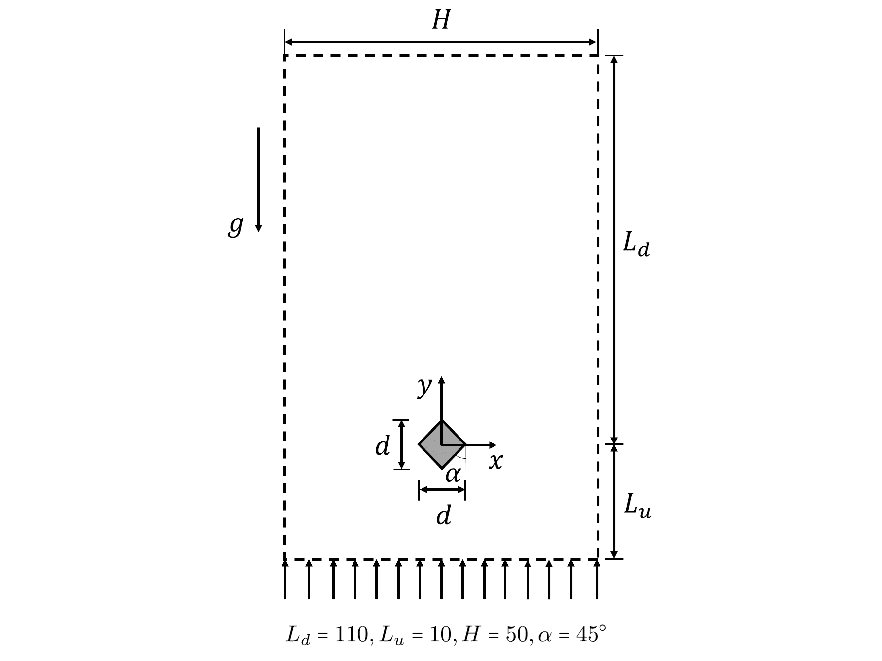
Figure 1: Two-dimensional computational domain.

II.2 Governing differential equations and boundary conditions

Two-dimensional, incompressible flow past a square cylinder at an angle of incidence $\alpha=45^{\circ}$ has been calculated. The governing differential equations, namely the continuity equation, the unsteady Navier-Stokes equations, and the energy equation, given in Equations 1, 2 and 3, respectively, are solved. In the dimensionless form, they are expressed as:

$$\pdv{u_{i}}{x_{i}}=0$$ (1)

$$\pdv{u_{i}}{\tau}+\pdv{(u_{j}u_{i})}{x_{j}}=-\pdv{p}{x_{i}}+\frac{1}{Re}\left[\pdv[order={2}]{u_{i}}{x_{i}}\right]+Ri\theta\delta_{i2}$$ (2)

$$\pdv{\theta}{\tau}+\pdv{(u_{i}\theta)}{x_{i}}=\frac{1}{RePr}\left[\pdv[order={2}]{\theta}{x_{i}}\right]$$ (3)

Where,

$$Gr=\dfrac{g\beta(T_{w}-T_{\infty})d^{3}}{\nu^{2}},\hskip 5.0ptRe=\dfrac{\rho V_{\infty}d}{\mu},\hskip 5.0ptRi=\dfrac{Gr}{Re^{2}},\hskip 5.0ptPr=\dfrac{\mu C_{ph}}{K}$$

$Gr$ is the Grashof number, $g$ is the acceleration due to gravity, $\beta$ is the coefficient of volumetric thermal expansion, $Pr$ is the Prandtl number of the fluid, $\nu$ is the kinematic viscosity of the fluid, $\rho$ is the density of the fluid, $\mu$ is the dynamic viscosity of the fluid, $C_{ph}$ is the specific heat of the fluid, and $K$ is the thermal conductivity of the fluid.

Air is the fluid under consideration and the Prandtl number is taken as 0.7. The effect of viscous dissipation has been neglected. The Boussinesq approximation has been utilized to convert density differences to corresponding temperature differences, and the buoyancy force term has been included in the $y$-momentum equation. In Equations 1, 2 and 3, all velocities and lengths are non-dimensionalized with the free-stream velocity $V_{\infty}$ and the projected length of the cylinder in the streamwise direction $d$, respectively. Similarly, time and pressure are non-dimensionalized with $d/V_{\infty}$ and $\rho V_{\infty}^{2}$, respectively. Temperature is non-dimensionalized as follows:

$$\theta=\dfrac{T-T_{\infty}}{T_{w}-T_{\infty}}$$ (4)

Where $T_{\infty}$ is the free-stream temperature, and $T_{w}$ is the temperature at the cylinder wall. The boundary conditions are as follows:

At the inlet ($Y=0$), constant streamwise velocity and temperature are used. Transverse velocity is set to zero.

$$v=V_{\infty},\hskip 5.0ptu=0$$

$$\ \theta=0$$

Transverse confining surfaces ($X=\pm H/2$) are unbounded and subsequently, they are modeled as free-slip, adiabatic surfaces.

$$\pdv{v}{x}=0,\hskip 5.0ptu=0$$

$$\pdv{\theta}{x}=0$$

At the outlet ($Y=L$), the selection of an appropriate outflow boundary condition is challenging because there is no unique prescription for the outflow boundary of external flows. It has been shown that the selection of the outflow boundary condition greatly affects upstream flow in external flows. Therefore, it should be chosen such that there is minimal effect on upstream flow. Accordingly, a convective boundary condition, first prescribed by Orlanski [32], has been employed for both velocity and temperature:

$$\pdv{u_{i}}{t}+v_{c}\pdv{u_{i}}{y}=0$$

$$\pdv{\theta}{t}+v_{c}\pdv{\theta}{y}=0$$

Where, $v_{c}$ is the average convective velocity of vortices leaving the domain. An optimum value of $v_{c}$ = 0.8 has been used for all calculations performed in the present study.

For the cylinder, no-slip and constant temperature boundary conditions are used for all surfaces.

$$u=v=0$$

$$\theta=1$$

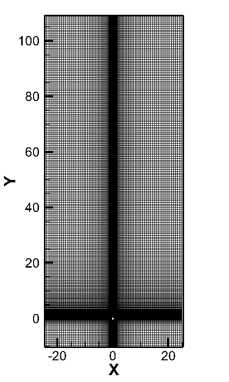
(a) Complete domain ($-25\leq$ X $\leq 25$, $-10\leq$ Y $\leq 110$)

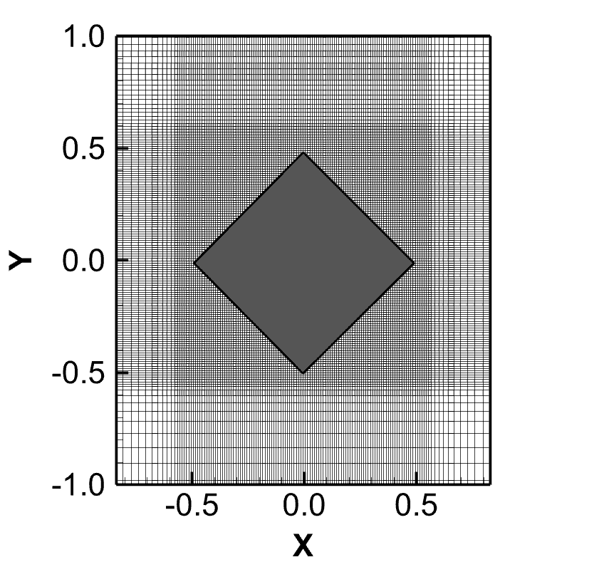
(b) Near the cylinder vicinity ($-1\leq$ X $\leq 1$, $-1\leq$ Y $\leq 1$)

Figure 2: Details of grid used in the (a) full domain, and (b) in the vicinity of the cylinder.

II.3 Solution Methodology

The numerical method used in the present work is an improved version of the finite-difference Marker and Cell algorithm proposed by Harlow and Welch [33]. The governing equations have been solved on a staggered grid without encountering the decoupling of pressure and velocity. Velocity components are located on the cell face to which they are normal and pressure is located at the cell center. Velocity components are interpolated to the cell center when required. Convective and diffusive terms are discretized using a second-order central difference scheme. Time advancement of both convective and diffusive terms is done using a second-order time accurate explicit Adams-Bashforth method.

A two-step predictor-corrector method is used to obtain the velocity and pressure fields. In the first step, provisional values of velocity are calculated explicitly using the results of the previous time step. In the subsequent step, pressure and velocity are corrected through the solution of Equations 7, 8 and 9 such that the resulting velocity field is divergence-free. This iterative procedure is continued till the velocity error between consecutive time steps is below a defined threshold.

The momentum equation can be written using a space operator G (containing convective and diffusive terms) as:

$$\pdv{u_{i}}{t}=G(u_{i},u_{j})-\pdv{p}{x_{i}}$$ (5)

Then, the predictor step for marching forward in time takes the form:

$$\frac{u_{i}^{*}-u_{i}^{n}}{\Delta t}=\left[\frac{3}{2}G(u_{i},u_{j})^{n}-\frac{1}{2}G(u_{i},u_{j})^{n-1}\right]-\pdv{p^{n}}{x_{i}}$$ (6)

Subsequently, the pressure correction step involves the solution of the pressure correction equation:

$$p^{\prime}=\dfrac{-\omega_{0}\pdv{u_{i}^{*}}{x_{i}}}{2\Delta t\left[\dfrac{1}{(\Delta x)^{2}}+\dfrac{1}{(\Delta y)^{2}}\right]}$$ (7)

The final solutions for pressure and velocity, as part of the correction step, are given as:

$$p^{n+1}\leftarrow p^{n}+p^{\prime}$$ (8)

$$u_{i}^{n+1}\leftarrow u_{i}^{*}+\dfrac{\Delta t}{\Delta x_{i}}p^{\prime}$$ (9)

The corrector step (Equation 7) is solved using point Gauss-Seidel method with an over relaxation parameter $\omega_{0}$, which accelerates pressure correction. An optimum value of $\omega_{0}$ = 1.8 has been used for all calculations in the present work.

The grid utilized is shown in Figure 2. It is a non-uniform, structured, Cartesian grid with a fine meshes in the near-wall region. In the vicinity of the cylinder, the grid is uniform with a cell size of $\Delta x=\Delta y=0.01$. Beyond a certain distance from the obstacle in all directions, the grid spacing is increased in a proper ratio to minimize computational cost.

The characteristics of flow and heat transfer past a bluff object are studied by calculating the different integral parameters. The vortex shedding frequency $f_{s}$ is calculated using the Fast Fourier transform (FFT) of any time signal in the wake. Subsequently, Strouhal number (St) is calculated as:

$$St=\dfrac{f_{s}d}{V_{\infty}}$$

The drag coefficient ($C_{D}$) and lift coefficient ($C_{L}$) are calculated as:

$$C_{D}=\dfrac{F_{D}}{\dfrac{1}{2}\rho V_{\infty}^{2}A_{x}}$$

$$C_{L}=\dfrac{F_{L}}{\dfrac{1}{2}\rho V_{\infty}^{2}A_{y}}$$

Nusselt number (Nu) can be written as:

$$\left.-K\pdv{T}{n}\right|_{n=0}=h(T_{w}-T_{\infty})$$

$$\implies Nu=\dfrac{hd}{K}=\left.-\pdv{\theta}{n}\right|_{n=0}$$

Where $f_{s}$ is the vortex shedding frequency, $F_{D}$ is the streamwise or drag force, $F_{L}$ is the transverse or lift force, $h$ is the wall heat transfer coefficient, $n$ is the wall normal direction to the surface of the cylinder, $A_{x}$ and $A_{y}$ are the streamwise and the transverse projected areas of the cylinder, respectively.

Rigorous validation has been performed for two different angles of incidence ($\alpha=0^{\circ}$ and $\alpha=45^{\circ}$) by comparing the time-averaged values of drag coefficient, the Strouhal number and the Nusselt number. Validation has been carried out against Sohankar et al. [3], Yoon et al. [27], Sharma and Eswaran [20], and Ranjan et al. [22]. The results of the validation are presented in Tables 1, 2, 3 and 4. For the $\alpha=0^{\circ}$ case, the mean drag coefficient reveals a maximum error of -3.09$\%$, while the corresponding errors in case of Strouhal number and Nusselt number are -1.85$\%$ and -5.37 $\%$, respectively. For the $\alpha=45^{\circ}$ case, the errors in the mean drag coefficient, Strouhal number, and Nusselt number are 5.16$\%$, 3.37$\%$, and -3.45$\%$, respectively. Therefore, the current simulated results are in good agreement with those available in the literature.

Table 1: Comparison of time-averaged drag coefficient and Strouhal number (isothermal flow, $\alpha=0^{\circ}$).

Reynolds number (Re)	Mean drag coefficient ($\overline{C}_{D}$)			Strouhal number (St)
	Present	Sohankar et al. [3]	Yoon et al. [27]	Present	Sohankar et al. [3]
50	1.57	1.62	1.57	0.114	-
100	1.43	1.46	1.44	0.147	0.147
150	1.41	1.41	1.40	0.159	0.162

Table 2: Comparison of mean Nusselt number at Re $=100$ ($\alpha=0^{\circ}$).

Richardson number (Ri)	Mean Nusselt number ($\overline{Nu}$)
	Present	Sharma and Eswaran [20]
0.0	3.87	4.09
0.25	4.12	4.30
0.50	4.37	4.55
0.75	4.55	4.73
1.0	4.70	4.87

Table 3: Comparison of time-averaged drag coefficient and Strouhal number (isothermal flow, $\alpha=45^{\circ}$).

Reynolds number (Re)	Mean drag coefficient ($\overline{C}_{D}$)			Strouhal number (St)
	Present	Sohankar et al. [3]	Yoon et al. [27]	Present	Sohankar et al. [3]
50	1.63	1.55	1.59	0.144	0.140
100	1.77	1.71	1.72	0.184	0.178
150	1.86	1.85	1.79	0.190	0.194

Table 4: Comparison of mean Nusselt number at Re $=100$ and Ri $=0.0$ ($\alpha=45^{\circ}$).

Reynolds number (Re)	Mean Nusselt number ($\overline{Nu}$)
	Present	Ranjan et al. [22]
60	4.00	4.08
100	5.20	5.35
150	6.43	6.66

The accuracy of the computed solution depends on the discretization error which is controlled by the grid resolution. To ensure that the grid is sufficiently fine to reduce the discretization error, the grid independence test has been carried out using three different grid sizes namely, G1 (619 $\times$ 320), G2 (777 $\times$ 396), and G3 (883 $\times$ 504) at Re $=100$ and Ri $=1.0$ by comparing the same parameters used in the validation. The parameters computed using the three grid sizes along with the minimum grid spacing in the vicinity of the cylinder are presented in Table 5. The domain size is kept constant for the grid independence test (120 $\times$ 50). Critical Ri has also been found for all three grids. In G1, it is 0.74, and in G2 and G3, it is 0.68. We observe that G2 produces results with minimal deviation from G3. The mean drag coefficient reveals an error of $2.82\%$ and $1.23\%$ for G1 and G2, respectively, with respect to G3. The corresponding error in case of Strouhal number is $2.09\%$ and $-5.88\%$, and for mean Nusselt number, it is $1.09\%$ and $0.55\%$, respectively. In view of moderate computational cost and closeness of results with G3, the grid G2 is utilized for all subsequent calculations.

Table 5: Mean drag coefficient, mean Nusselt number and Strouhal number for different grid resolutions at Re $=100$ and Ri $=1.0$.

Grid	Minimum spacing	Mean drag coefficient ($\overline{C}_{D}$)	Mean Nusselt number ($\overline{Nu}$)	Strouhal number (St)
G1	0.025	2.48	5.50	0.215
G2	0.01	2.44	5.47	0.221
G3	0.0075	2.41	5.44	0.234

As mentioned in Section I, integral parameters depend on the blockage ratio. To ensure that the calculated integral parameters are free from dependence on blockage ratio, the domain independence test has been carried out using two different domains, namely D1 ($120\times 50$, $\beta=2\%$) and D2 ($120\times 67$, $\beta=1.5\%$) at Re $=100$ and Ri $=1.0$ by comparing the same parameters that are used in the validation. Both domains have the same streamwise extent. As the original domain is already very long, it is expected that an increase in its length downstream of the cylinder will not change the flow physics. A detailed investigation on the effect of the domain length has been conducted by Dushe [17]. The parameters calculated using the two domains are presented in Table 6. The mean drag coefficient reveals an error of $0.4\%$ for D1 with respect to D2, whereas for mean Nusselt number and Strouhal number, it is $0.6\%$, and $6.8\%$, respectively. The domain independence test reveals that the results do not depend on blockage. Therefore, domain D1 is used for all subsequent calculations.

Table 6: Mean drag coefficient, mean Nusselt number and Strouhal number for different domain sizes at Re $=100$ and Ri $=1.0$.

Domain	Mean drag coefficient ($\overline{C}_{D}$)	Mean Nusselt number ($\overline{Nu}$)	Strouhal number (St)
D1 ($120\times 50$)	2.44	5.47	0.221
D2 ($120\times 67$)	2.45	5.44	0.237

III Results and Discussion

In this section, we use the results of DNS to provide insight into the effect of buoyancy on the flow field behind the cylinder. Based on the instantaneous and time-averaged results, we discuss the physical mechanisms for the suppression of vortex shedding, vorticity inversion, and the far-field unsteadiness. The Stuart-Landau model has been employed to accurately estimate the critical Richardson number for the suppression of vortex shedding in the near-field. We have also discussed the effect of buoyancy on the integral parameters of the flow field. The results obtained are only applicable to the streamwise length of the domain used in the current study. The choice of domain length influences the observed transitions, and it is possible that a longer domain could reveal additional flow physics. To achieve statistical independence, we set the total averaging time (T) to different values for different calculations. It is found that the results obtained do not vary more than $2\%$ between two different averaging times. Therefore, it is expected that the presented results are statistically independent.

III.1 Instantaneous flow

Instantaneous vorticity and temperature contours for Re $=100$ and $0.0\leq$ Ri $\leq 1.0$ are presented in Figures 3 and 5 for the full domain and Figures 4 and 6 in the vicinity of the cylinder, respectively. All instantaneous contours are phase-synchronized to ensure uniformity in flow visualization. The instantaneous vorticity contours (see Figure 3) reveal the presence of vortex shedding and the Bénard-von Kármán vortex street in the near-field for Ri $=0.0$ (forced convection). With the absence of the buoyancy-driven flow, the flow field resembles that of forced flows, showing negative vorticity in the left half and positive vorticity in the right half, which spans the entire domain downstream. The two oppositely-signed shear layers attached to the cylinder cross the centerline alternatively during a shedding cycle and interact with each other, leading to the shedding of vortices. In the far-field, the flow is steady at Ri $=0.0$. When Ri is increased to 0.2, it is seen that the sign of vorticity starts out as that of a forced flow but slowly inverts beyond a critical distance downstream and persists with this inverted sign for the rest of the domain beyond the critical distance. Additionally, the far-field flow is no longer steady as it was in the Ri $=0.0$ case. At higher Ri (0.4-0.7), the inversion of vorticity takes place closer to the cylinder, and the width between the two shear layers increases downstream. The shape of the shed vortices also differs greatly with increasing Ri, which requires further investigation. For Ri $\geq$ 0.7, the near-field flow becomes steady with the suppression of vortex shedding by buoyancy, and a large-scale undulation of the shear layers is seen in the far-field region. The shear layer becomes discontinuous, leading to the formation of isolated patches of vorticity due to the instability developing within the stronger shear layer. As Ri increases, the inception point of the far-field unsteadiness moves closer to the cylinder. The instantaneous vorticity in the cylinder vicinity (see Figure 4) shows regular vortex shedding at Ri $=0.0$ with vortices of opposite sign being shed alternatively into the wake. With increasing Ri, the transverse extent of the interaction of the positively-signed shear layer with the oppositely-signed shear layer reduces gradually, appearing as though their mutual interaction is being inhibited. For Ri $>$ 0.7, there is no interaction between the oppositely-signed shear layers, and they form a separation bubble, similar to forced flows below the critical Re at which the transition to unsteadiness occurs. Vortex shedding does not occur for Ri $>$ 0.7 and the point of inversion of vorticity comes so close to the cylinder that it can be visualized in the near-field plots of vorticity as well (see Figures 4(e) and 4(f)). Isotherms reveal the presence of vortex shedding in the near-field for Ri $=0.0$ and the far-field is steady, as confirmed through the examination of signals of temperature, even though small oscillations are noticeable in the isotherm (see Figure 5). At Ri $=0.2$, the undulation of shear layers extends to Y $=65$ and the complete flow field is unsteady up to Ri $=0.6$. The shape of the isotherm structures continues to change when Ri is increased, due to the increased strength of the buoyancy force and the constant strength of the inertial force. With further increase in Ri, the temperature in the near-field is steady, and the far-field reveals the presence of structures similar to those seen in plumes, as shown by Kimura and Bejan [31]. The near-field plots of temperature show similar behavior as the vorticity contours (see Figure 6). The undulation of the isotherms is significantly lower at higher Ri, and for Ri $\geq$ 0.7, the structures reveal a steady flow in the near-field.

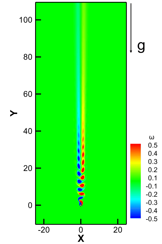
(a) Ri $=0.0$

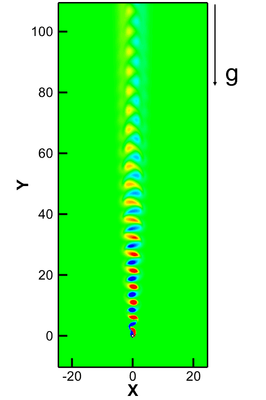
(b) Ri $=0.2$

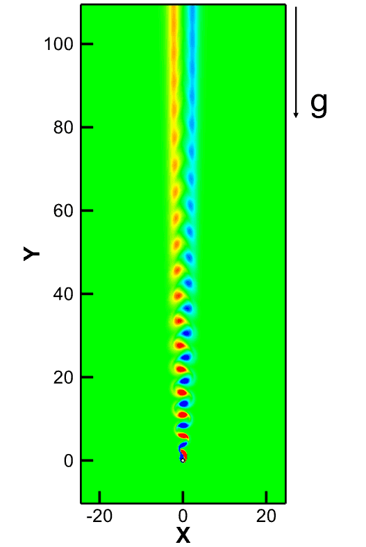
(c) Ri $=0.4$

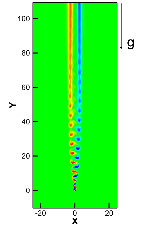
(d) Ri $=0.6$

(e) Ri $=0.7$

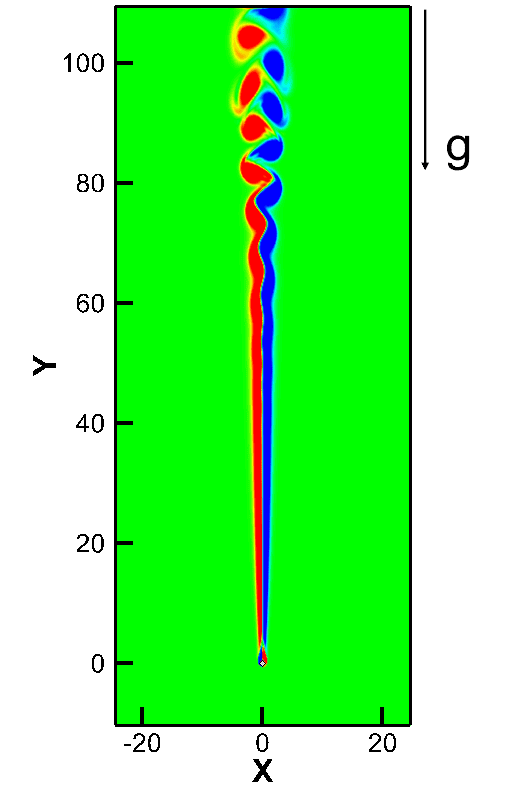
(f) Ri $=1.0$

Figure 3: Instantaneous vorticity contours for Re $=100$ and $0.0\leq$ Ri $\leq 1.0$: (a) Ri $=0.0$, (b) Ri $=0.2$, (c) Ri $=0.4$, (d) Ri $=0.6$, (e) Ri $=0.7$, (f) Ri $=1.0$.

(a) Ri $=0.0$

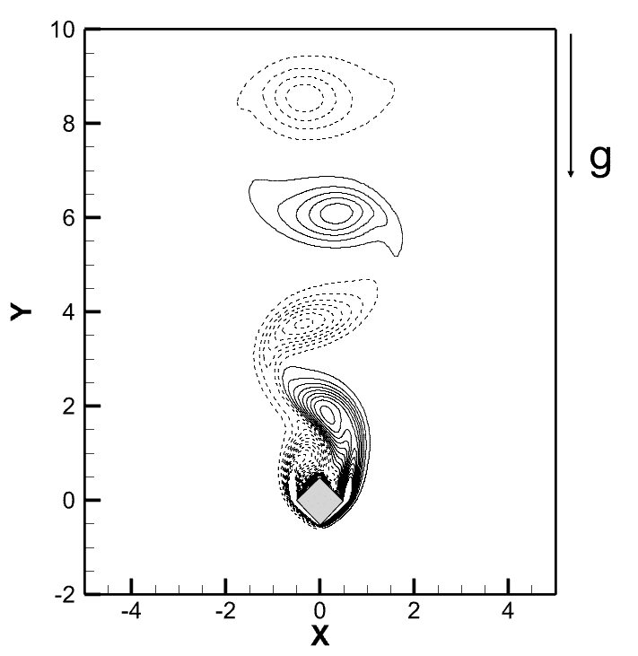
(b) Ri $=0.2$

(c) Ri $=0.4$

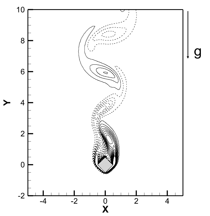
(d) Ri $=0.6$

(e) Ri $=0.7$

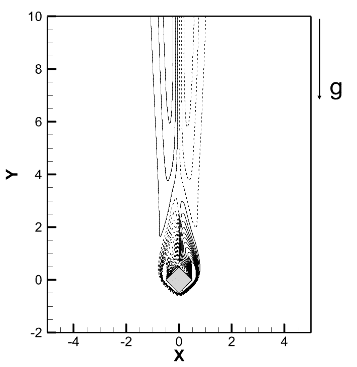
(f) Ri $=1.0$

Figure 4: Instantaneous vorticity contours (in the cylinder vicinity) for Re $=100$ and $0.0\leq$ Ri $\leq 1.0$: (a) Ri $=0.0$, (b) Ri $=0.2$, (c) Ri $=0.4$, (d) Ri $=0.6$, (e) Ri $=0.7$, (f) Ri $=1.0$; ($\overline{\omega}_{Z,min},\overline{\omega}_{Z,max},\Delta\overline{\omega}_{Z})\equiv(-5,5,0.4)$.

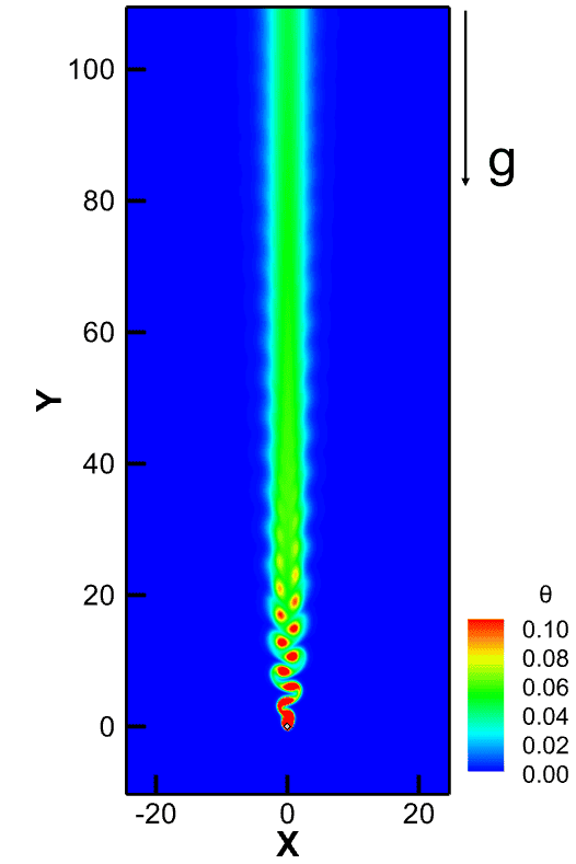
(a) Ri $=0.0$

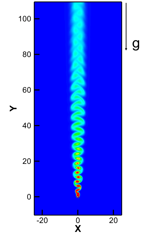
(b) Ri $=0.2$

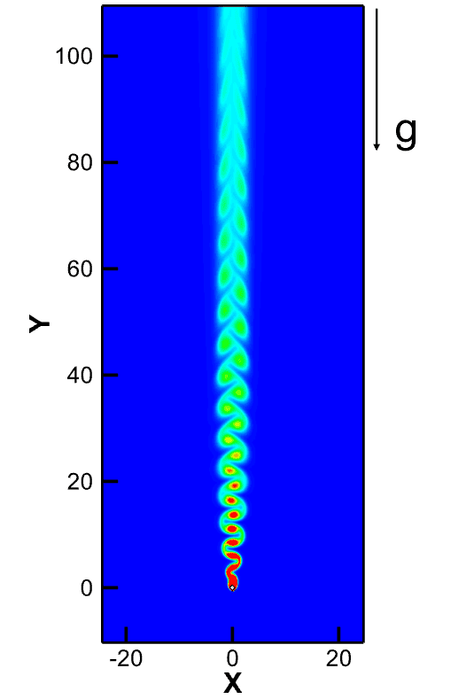
(c) Ri $=0.4$

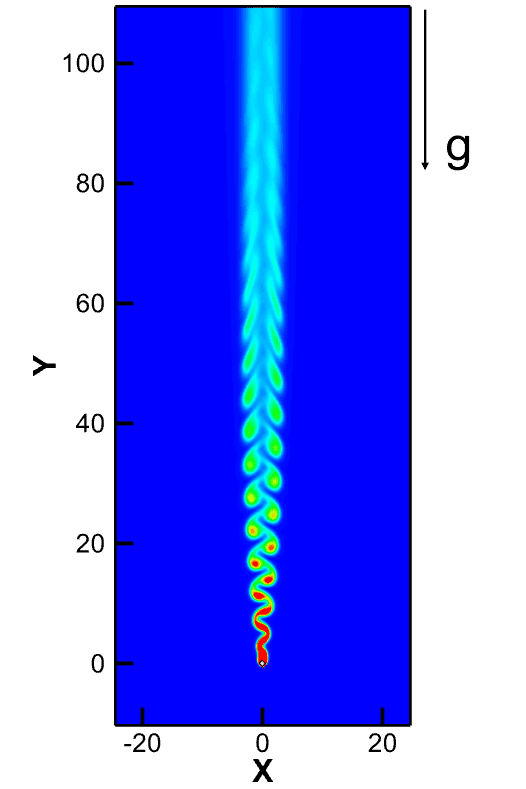
(d) Ri $=0.6$

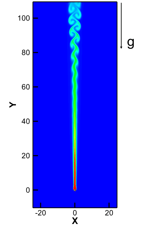
(e) Ri $=0.7$

(f) Ri $=1.0$

Figure 5: Instantaneous temperature contours for Re $=100$ and $0.0\leq$ Ri $\leq 1.0$: (a) Ri $=0.0$, (b) Ri $=0.2$, (c) Ri $=0.4$, (d) Ri $=0.6$, (e) Ri $=0.7$, (f) Ri $=1.0$.

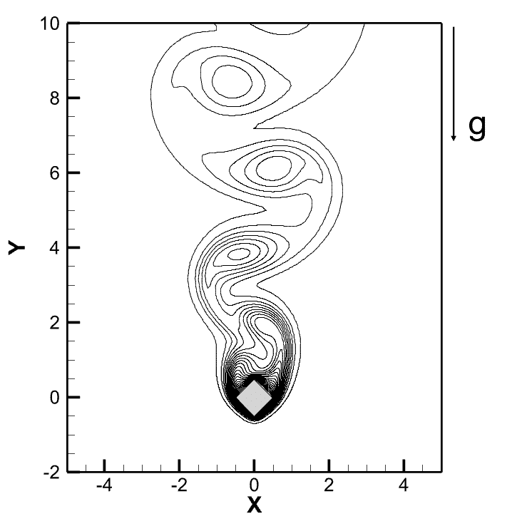
(a) Ri $=0.0$

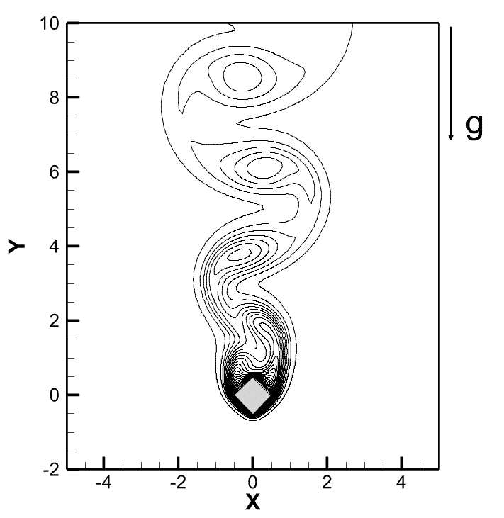
(b) Ri $=0.2$

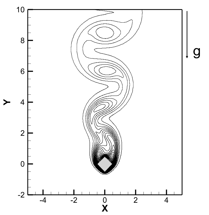
(c) Ri $=0.4$

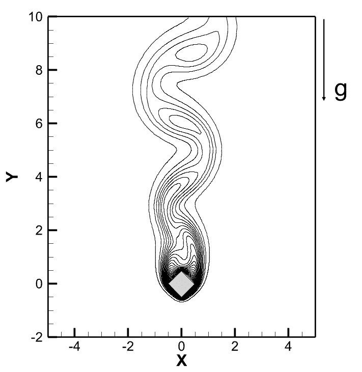
(d) Ri $=0.6$

(e) Ri $=0.7$

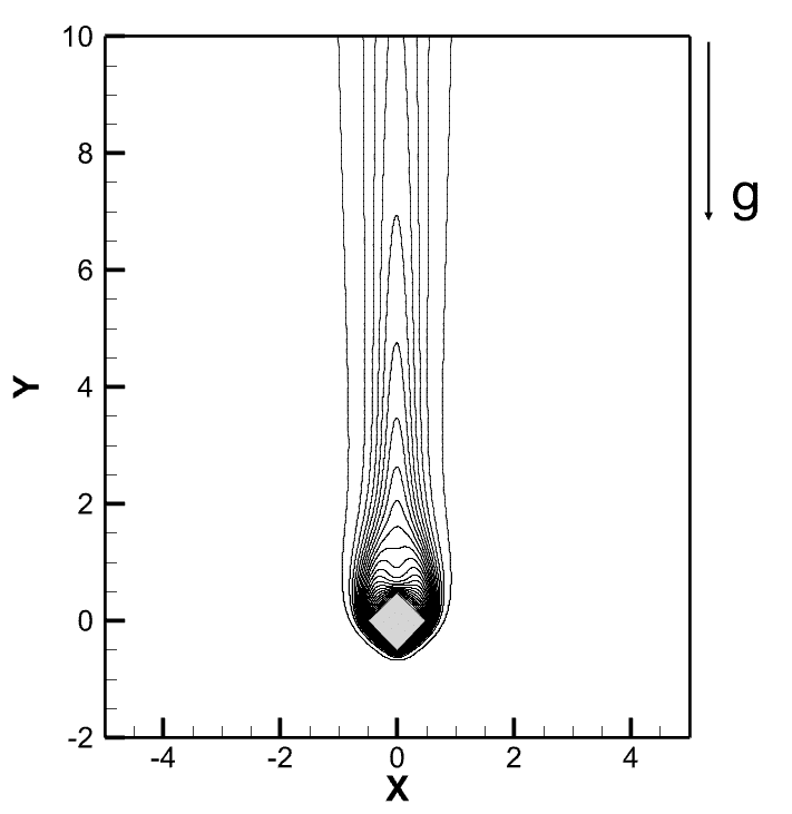
(f) Ri $=1.0$

Figure 6: Instantaneous temperature contours (in the cylinder vicinity) for Re $=100$ and $0.0\leq$ Ri $\leq 1.0$: (a) Ri $=0.0$, (b) Ri $=0.2$, (c) Ri $=0.4$, (d) Ri $=0.6$, (e) Ri $=0.7$, (f) Ri $=1.0$; ($\overline{\theta}_{min},\overline{\theta}_{max},\Delta\overline{\theta})\equiv(0.01,1,0.041)$.

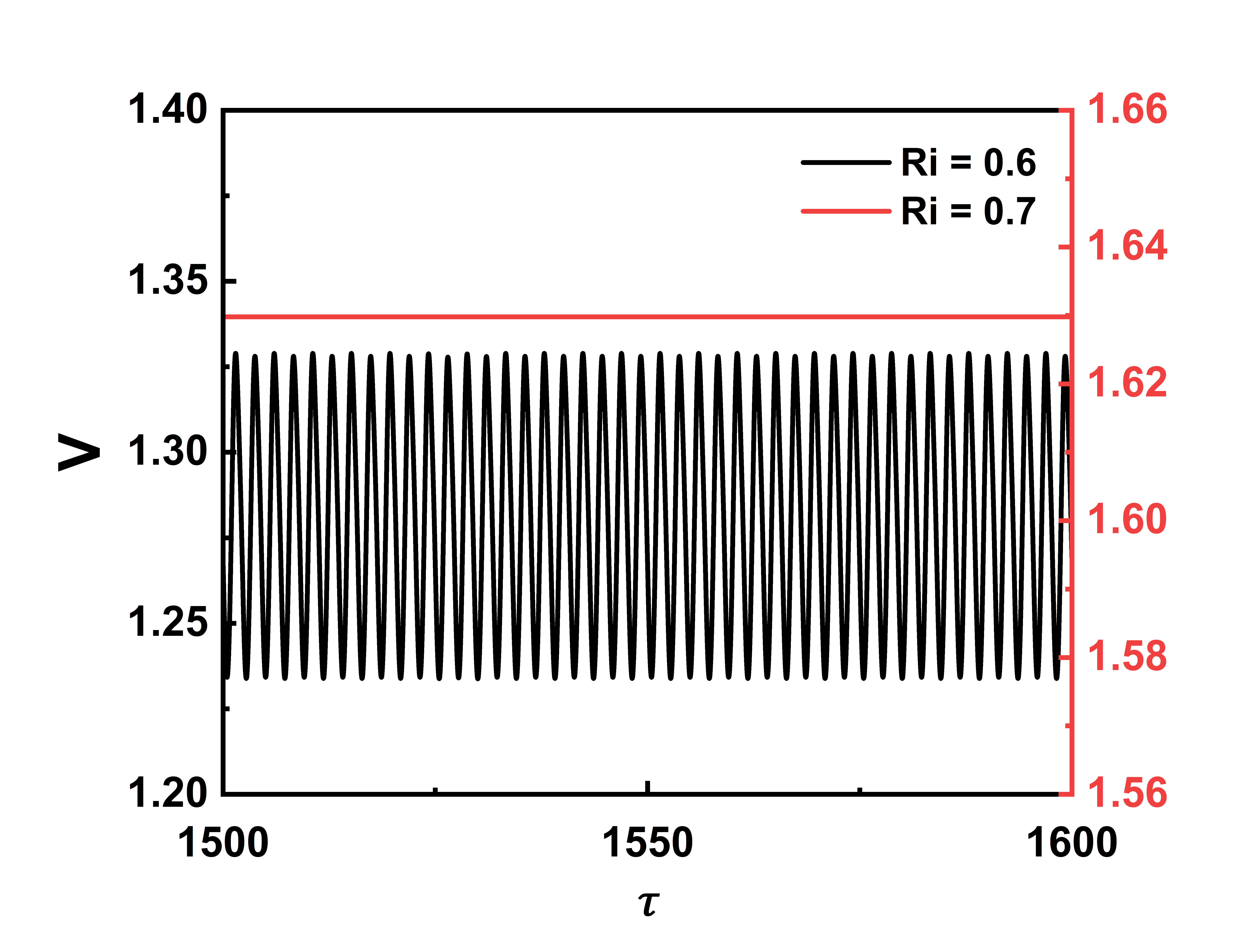
(a) Y $=11.5$

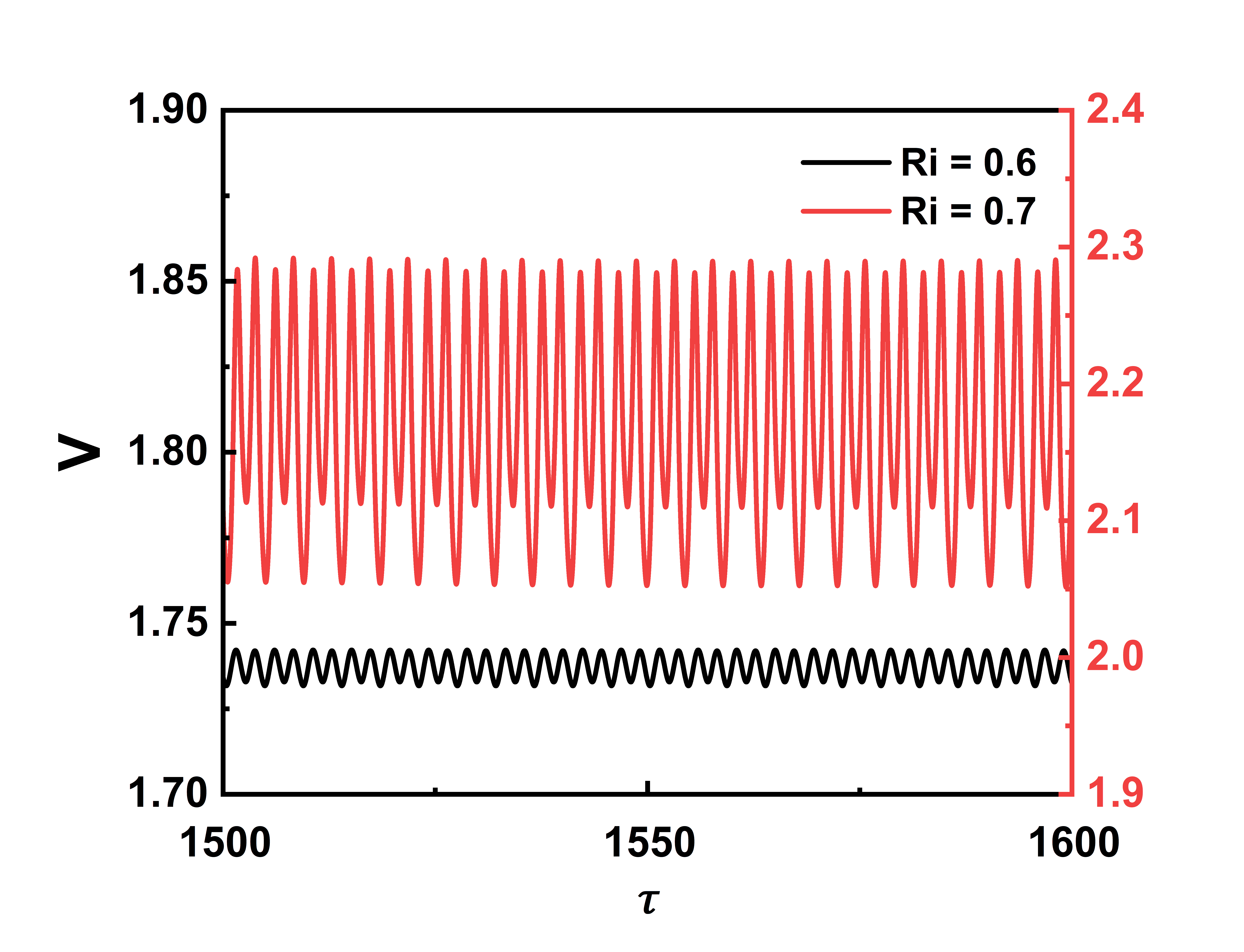
(b) Y $=73.5$

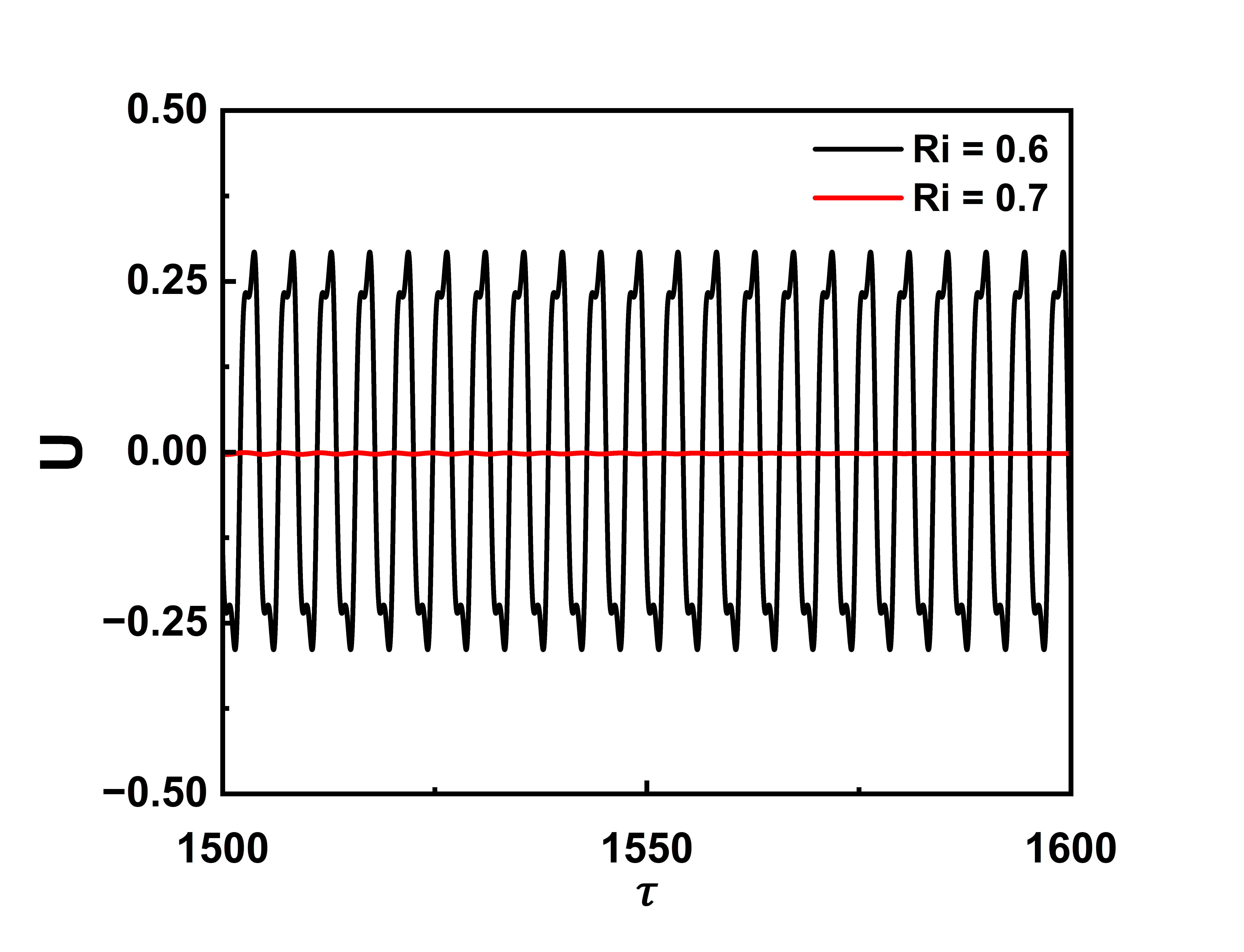
(c) Y $=11.5$

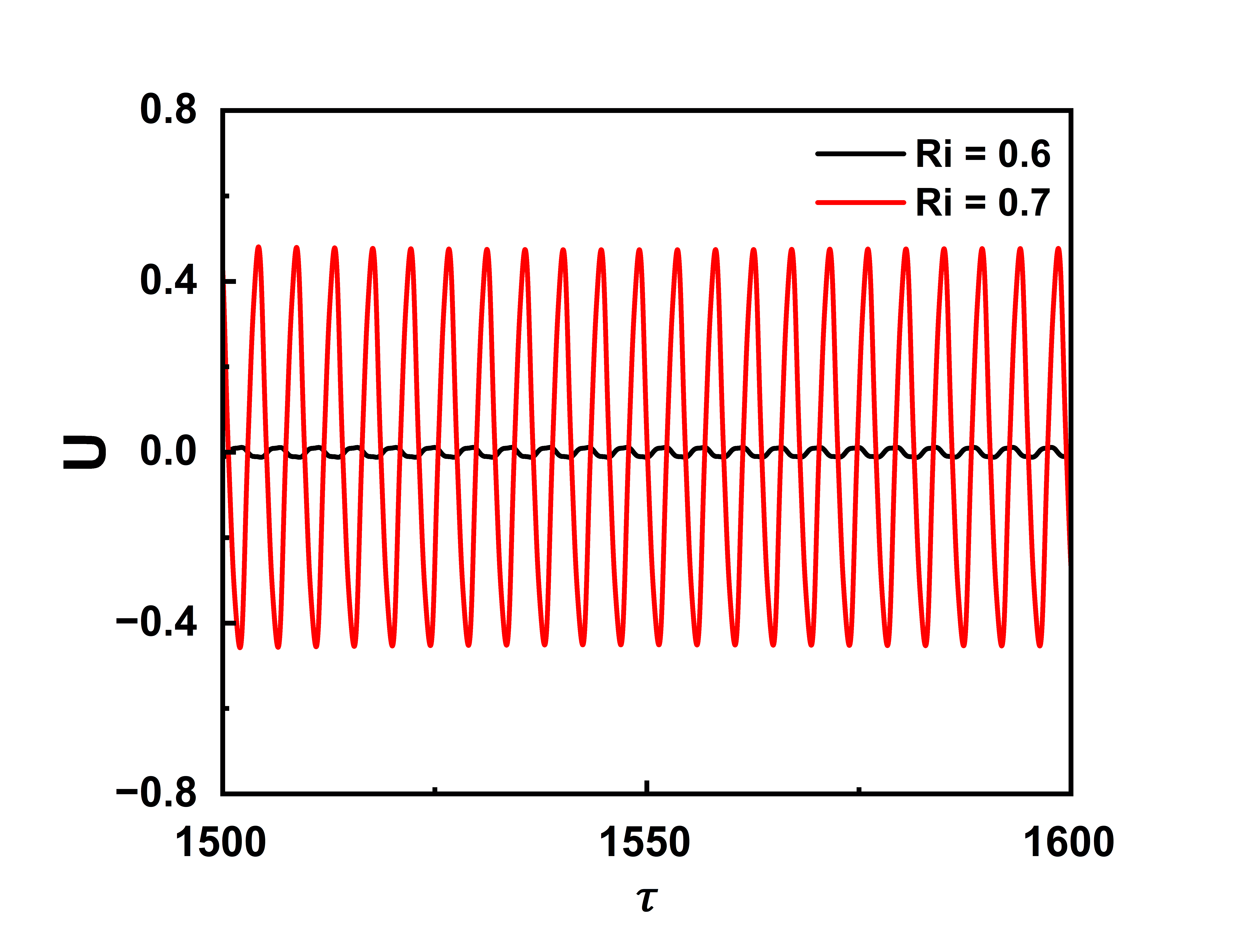
(d) Y $=73.5$

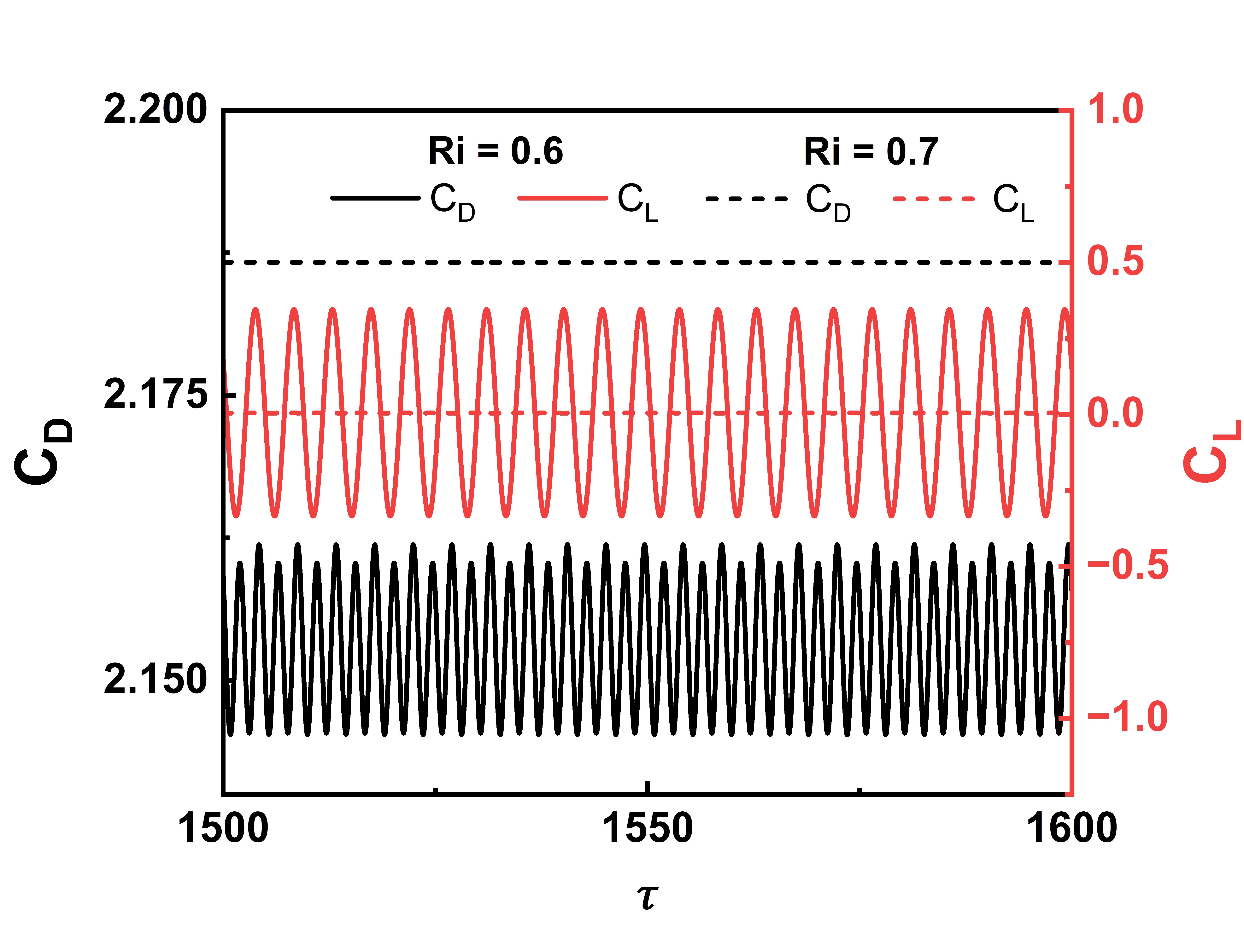
(e) Lift and drag coefficient signals

Figure 7: Streamwise (a, b) and transverse (c, d) velocity signals in the near- and far-field for Ri $=0.6$ and Ri $=0.7$, along with (e) drag and lift coefficient signals. The near-field signals reveal the suppression of vortex shedding and the far-field signals show the far-field unsteadiness, while the force coefficient signals characterize the near-field flow excellently.

To confirm the behavior shown by the flow field in the contours, we have plotted time signals of the streamwise and transverse velocity in the near-field (Y $=11.5$) and far-field (Y $=73.5$), which are shown in Figure 7 for Ri $=0.6$ and Ri $=0.7$. For Ri $=0.6$, streamwise and transverse velocity plots in the near-field reveal unsteady, periodic behavior, and for Ri $=0.7$, steady behavior without any periodicity is observed (see Figures 7(a) and 7(c)). Far-field streamwise and transverse velocity plots show the opposite behavior, with mild unsteadiness in the case of Ri $=0.6$ associated with increasing plume-like behavior and large-scale unsteadiness for Ri $=0.7$ associated with the onset of the far-field plume-like unsteadiness (see Figures 7(b) and 7(d)). There is a large difference in the amplitude of the signals between Ri $=0.6$ and Ri $=0.7$, which confirms that the unsteadiness in the far-field is not due to the shedding of vortices in the near-field, the strength of which dissipates significantly due to viscous diffusion as it reaches the far-field, which can be seen in the Ri $=0.6$ signals. In both regions (near-field and far-field), the streamwise velocity signal has a frequency that is twice that of the transverse velocity signal. Interestingly, in the near-field, U exhibits multiple frequencies, while V has a unique frequency. In the far-field, V exhibits multiple frequencies, while U has a unique frequency, demonstrating an opposite behavior to that of the near-field. It appears that such behavior is characteristic of the wake nature of the near-field and the plume nature of the far-field; however, this requires further investigation. The plots of lift and drag coefficient (see Figure 7(e)) show similarities with the near-field velocity signals, suggesting that the near-field flow is unsteady for Ri $=0.6$ and steady for Ri $=0.7$, supporting the suppression of vortex shedding in the near-field. This makes the force coefficients excellent predictors of the nature of the near-field flow. The skin friction drag and Nusselt number are analogous quantities in that they are both proportional to the gradient of velocity and temperature, respectively. Similar to the variation in friction drag, which is negligible, the fluctuation in Nu is also very small, even though its time-averaged value is very large. Therefore, Nu has not been plotted as a function of time, as there are negligible fluctuations in Nu for all Ri.

Table 7: Variation of Strouhal number (St) with Richardson number (Ri) in the near-field (Y $=11.5$) and far-field (Y $=73.5$). The transverse velocity signal along the centerline (X $=0$) has been used for the calculation of Strouhal number.

Richardson number (Ri)	Strouhal number (St)
	Near-field (Y $=11.5$, X $=0$)	Far-field (Y $=73.5$, X $=0$)
0.0	0.180	0.0
0.2	0.197	0.194
0.4	0.207	0.204
0.6	0.220	0.220
0.7	-	0.227
1.0	-	0.221

Table 7 shows the variation of Strouhal number (St) with Ri. The transverse velocity signal along the centerline (X $=0$) is used to compute the Strouhal number at two different streamwise locations, Y $=11.5$ and Y $=73.5$ which fall in the near-field and far-field, respectively. St shows negligible variation between the near-field and far-field for Ri $<$ 0.7. Above the critical Ri, the near-field flow has no periodicity and the corresponding St is zero. The flow in the wake is accelerated due to the buoyancy force, which is more significant at elevated Richardson numbers, resulting in increased Strouhal number with increasing Ri.

III.2 Stuart-Landau Analysis

In DNS, we are able to identify the critical Ri correct to a certain precision due to the discrete increments of the control parameter (here, Ri) taken during calculations. The Stuart-Landau model enables accurate identification of the critical Ri. This model is well-known for describing the behavior of nonlinear dynamical systems near the Hopf bifurcation. The derivation of this equation from the hydrodynamic equations has been provided in many previous works [34, 35, 36, 37]. The Landau model has been shown to accurately describe the transition to periodicity in the wake of flows past cylinders by several authors in the literature [3, 38, 39]. It has been shown earlier by Dushe [17] that the two transitions obtained for mixed convection past a square cylinder at $\alpha=0^{\circ}$ are both Hopf bifurcations. Dushe also showed that the Stuart-Landau model is suitable for the prediction of the critical Ri for vortex shedding suppression in the wake of mixed convective flows past cylinders. The Stuart-Landau equation describes the perturbation near the bifurcation as follows:

$$\odv{A}{t}=\sigma A-\dfrac{l}{2}A|A|^{2}$$ (10)

Where $A$ is any characteristic complex amplitude associated with the fundamental frequency, $\sigma$ is the linear growth rate, and $l$ is the first Landau constant. It can be shown that the equilibrium amplitude ($A_{e}$) of oscillations near the bifurcation varies with the control parameter (Ri) as:

$$A_{e}^{2}=C(Ri-Ri_{c})$$ (11)

Where $Ri_{c}$ is the critical Richardson number and C is a constant. Equilibrium amplitudes of the characteristic quantity around the (approximate) critical Richardson number can be plotted and fitted to this equation. The intercept of the best-fit line with the Ri axis yields the critical Richardson number.

For selecting the most appropriate characteristic quantity, we have plotted the mean-to-peak amplitudes of different quantities ($C_{L}$, $C_{D}$, $v$, $u$, $\theta$) against Ri, below the approximate critical Ri and fitted a linear curve to the data. Based on this, we have found that the lift coefficient produces the best fit in terms of the coefficient of determination ($R^{2}$) as well as closeness to the critical Ri predicted by DNS. Therefore, we have used the lift coefficient signal for estimation of the near-field transition point. The Landau model is applicable only for those Ri very close to the critical Ri as it is a linearized model. Therefore, we have considered the equilibrium amplitudes of the lift coefficient for Ri in the range (0.64-0.68) in increments of 0.01. The square of the equilibrium amplitude ($A_{e}^{2}$) of the lift coefficient signal has been plotted against Ri along with the best-fit line in Figure 8. The critical Ri determined from the Landau model comes out to be 0.681. The corresponding value obtained by Arif and Hasan [28] is 0.78 which is different from our result. This may be due to a different discretization in the computational method or the short domain taken by the authors.

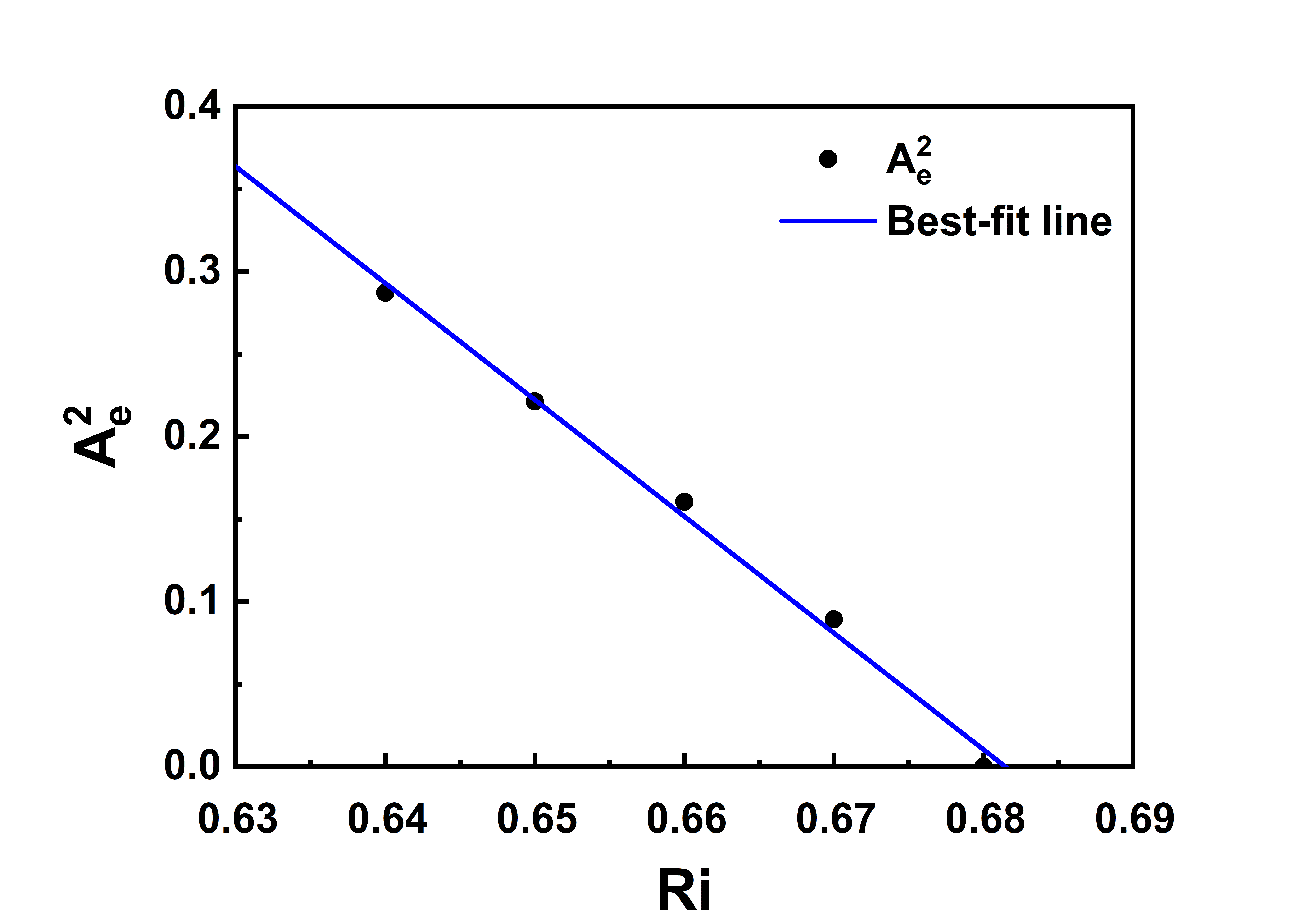
Figure 8: Variation of $A_{e}^{2}$ of the lift coefficient signal with Richardson number.

III.3 Time-averaged flow

Time-averaged vorticity and temperature contours for Re $=100$ and $0.0\leq$ Ri $\leq 1.0$ are presented in Figures 9 and 11 in the full domain and Figures 10 and 12 in the vicinity of the cylinder, respectively. The time-averaged vorticity contours in the complete domain (see Figure 9) reveal that at Ri $=0.0$, the strength of the vorticity is high in the near-field but diminishes in the far-field, while for Ri $>$ 0.0, the strength of the vorticity is weak in the near-field but grows on moving downstream, showing the opposite nature of the forced convective vorticity and the natural convective vorticity. The forced convective vorticity is introduced due to the shear layer separation at the lateral corners of the cylinder, while the natural convective vorticity is introduced due to the buoyancy-driven flow, which causes a jetting effect. The interplay of these opposing vorticities is the cause of many physical phenomena that we have observed in this study and will be discussed in detail later. Beyond Ri $=0.7$, the strength of the vorticity is significantly higher than that of the cases below Ri $=0.7$, and the oppositely-signed vortices remain attached up to the far-field, which was not the case at lower Ri. Further, the two vortices separate suddenly in the far-field at a point (around Y $=65$) which also coincides with the point of onset of the far-field unsteadiness. All positive Ri cases display vorticity inversion as seen in the instantaneous contours earlier. In the near-field plot of vorticity, the width between the shear layers is seen to reduce with increasing Ri, similar to the instantaneous case. Beyond Ri $=0.7$, the inversion can be seen in the near-field, and the vortices form a steady recirculation bubble, whose length decreases with increasing Ri, and these cases resemble the instantaneous plots as the flow is steady in the near-field. Time-averaged temperature contours (see Figure 11) show a widening of the plume in the near and intermediate fields for Ri $<$ 0.7. Beyond 0.7, the plume is narrow in the near-field, and there is a sharp increase in the plume width in the far-field, associated with the onset of the far-field unsteadiness. Such behavior is also observed in the near-field temperature contours (see Figure 12), where the plume is wide in the near-field for low Ri, and beyond Ri $=0.7$, the plume is narrow.

(a) Ri $=0.0$

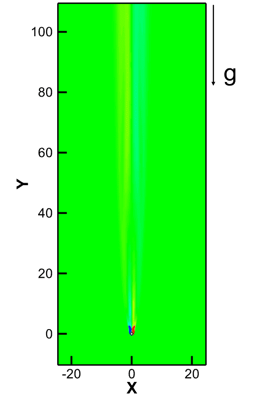
(b) Ri $=0.2$

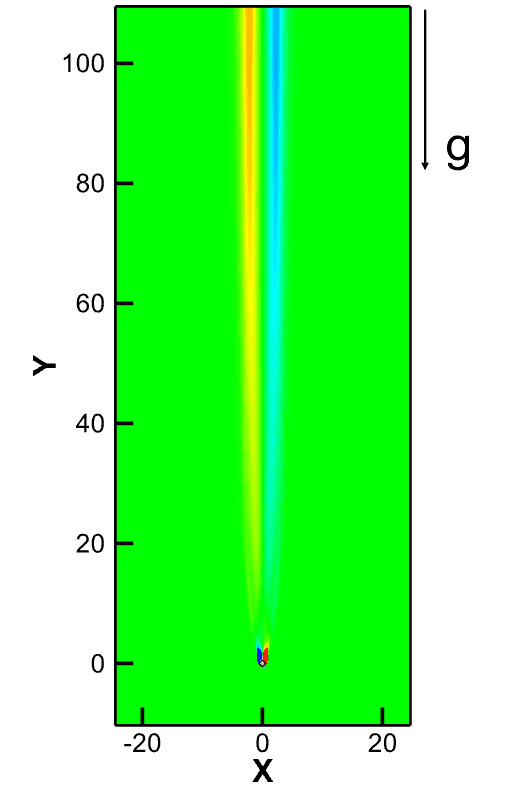
(c) Ri $=0.4$

(d) Ri $=0.6$

(e) Ri $=0.7$

(f) Ri $=1.0$

Figure 9: Time-averaged vorticity contours for Re $=100$ and $0.0\leq$ Ri $\leq 1.0$: (a) Ri $=0.0$, (b) Ri $=0.2$, (c) Ri $=0.4$, (d) Ri $=0.6$, (e) Ri $=0.7$, (f) Ri $=1.0$.

(a) Ri $=0.0$

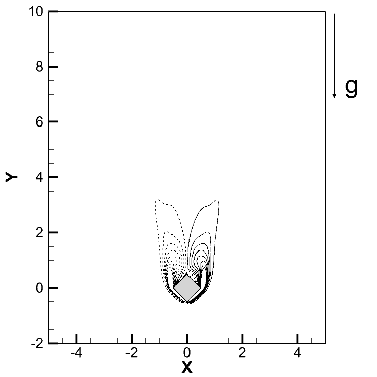
(b) Ri $=0.2$

(c) Ri $=0.4$

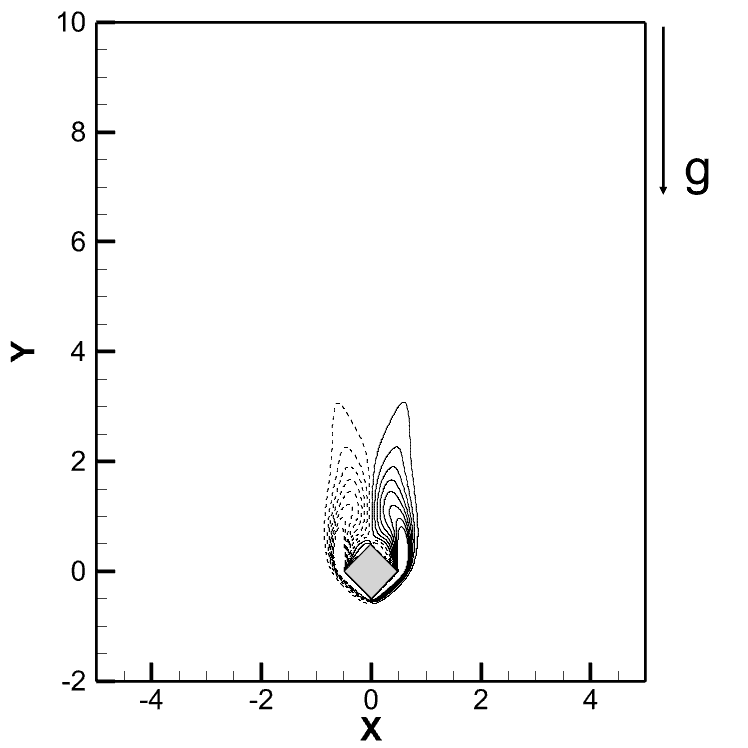
(d) Ri $=0.6$

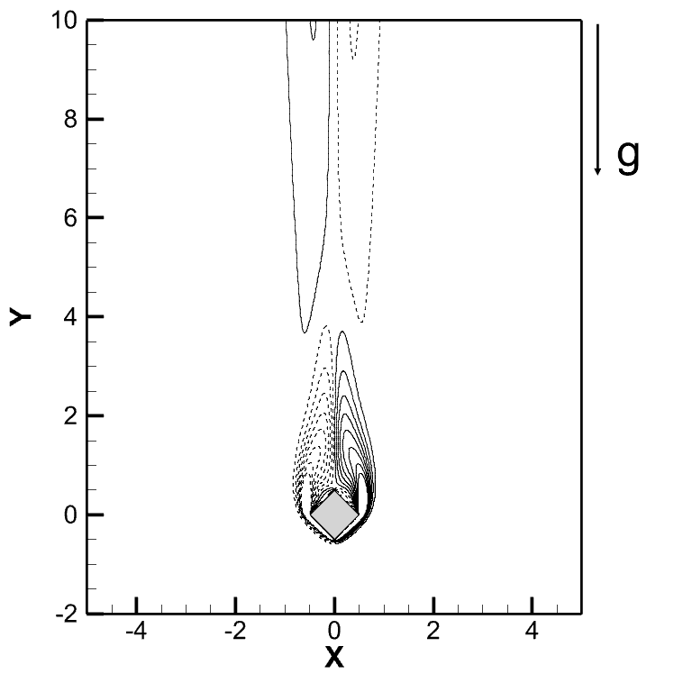
(e) Ri $=0.7$

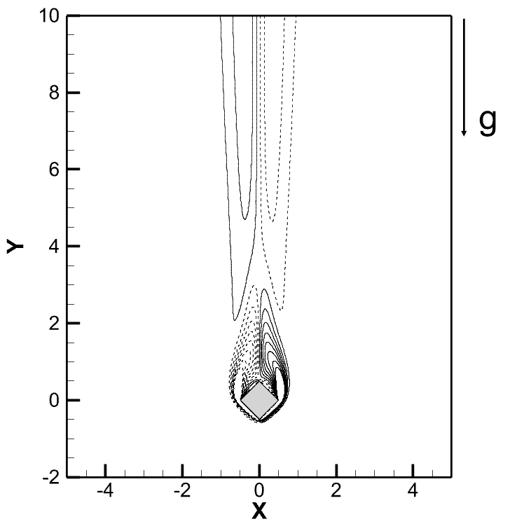
(f) Ri $=1.0$

Figure 10: Time-averaged vorticity contours (in the cylinder vicinity) for Re $=100$ and $0.0\leq$ Ri $\leq 1.0$: (a) Ri $=0.0$, (b) Ri $=0.2$, (c) Ri $=0.4$, (d) Ri $=0.6$, (e) Ri $=0.7$, (f) Ri $=1.0$; ($\overline{\omega}_{Z,min},\overline{\omega}_{Z,max},\Delta\overline{\omega}_{Z})\equiv(-4,4,0.53)$.

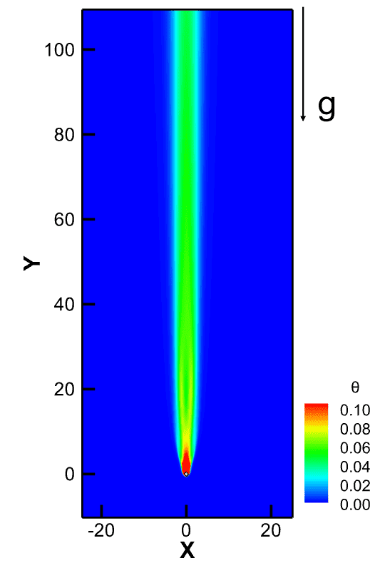
(a) Ri $=0.0$

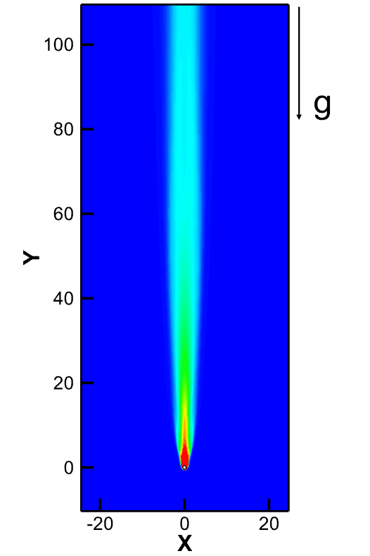
(b) Ri $=0.2$

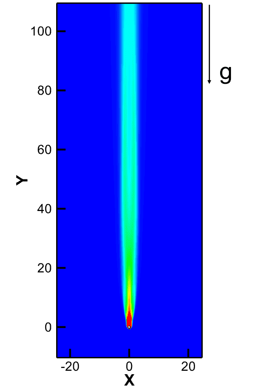
(c) Ri $=0.4$

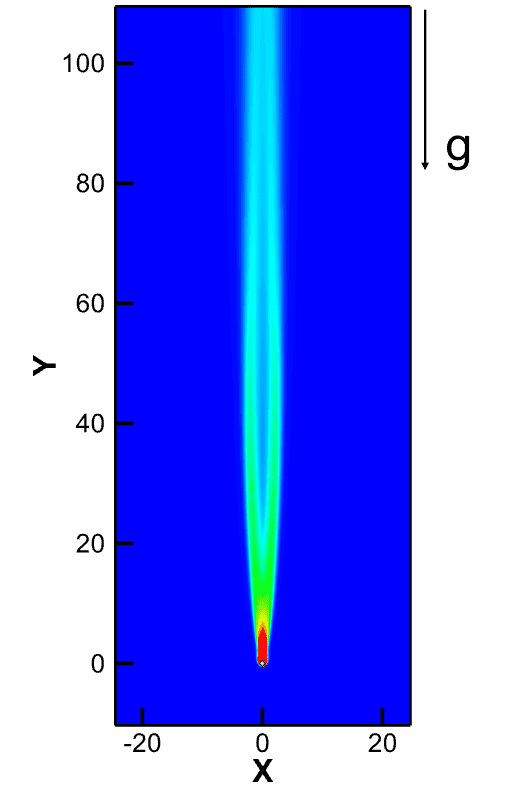
(d) Ri $=0.6$

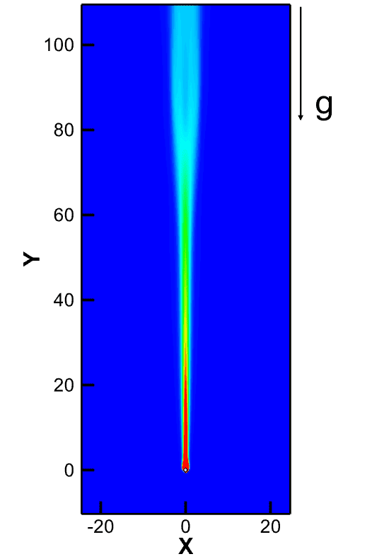
(e) Ri $=0.7$

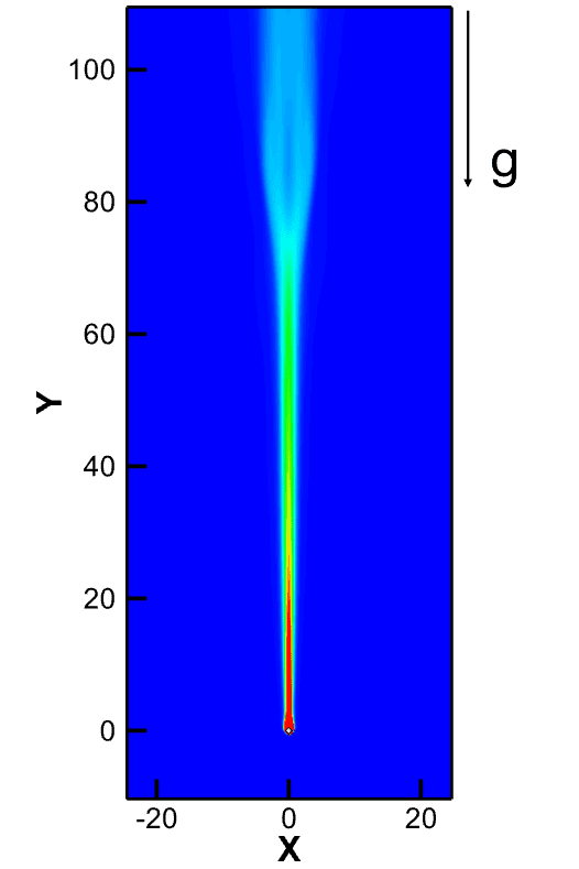
(f) Ri $=1.0$

Figure 11: Time-averaged temperature contours for Re $=100$ and $0.0\leq$ Ri $\leq 1.0$: (a) Ri $=0.0$, (b) Ri $=0.2$, (c) Ri $=0.4$, (d) Ri $=0.6$, (e) Ri $=0.7$, (f) Ri $=1.0$.

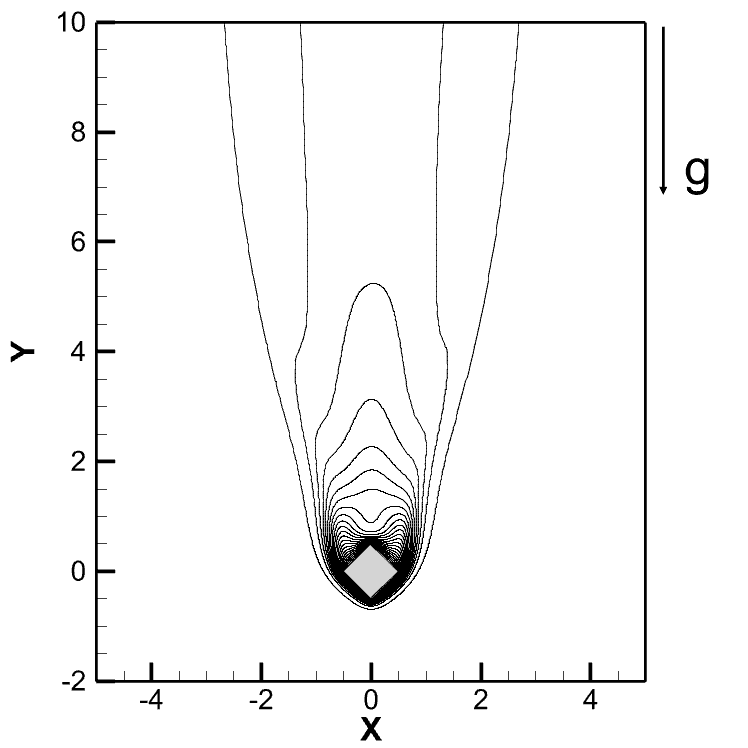
(a) Ri $=0.0$

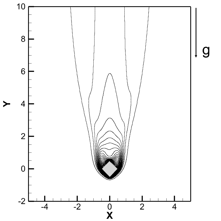
(b) Ri $=0.2$

(c) Ri $=0.4$

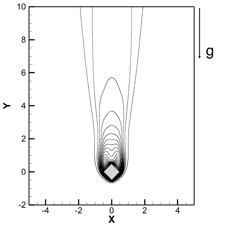
(d) Ri $=0.6$

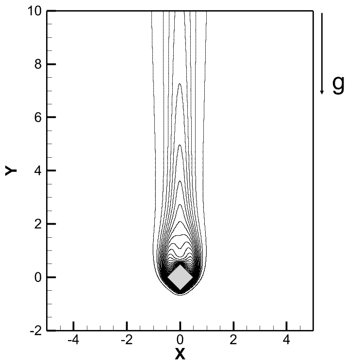
(e) Ri $=0.7$

(f) Ri $=1.0$

Figure 12: Time-averaged temperature contours (in the cylinder vicinity) for Re $=100$ and $0.0\leq$ Ri $\leq 1.0$: (a) Ri $=0.0$, (b) Ri $=0.2$, (c) Ri $=0.4$, (d) Ri $=0.6$, (e) Ri $=0.7$, (f) Ri $=1.0$, ($\overline{\theta}_{min},\overline{\theta}_{max},\Delta\overline{\theta})\equiv(0.01,1,0.041)$

Figure 13 shows the centerline streamwise velocity and centerline temperature along the streamwise length of the domain for different Ri. Figure 13(a) reveals the buoyancy-driven jetting effect, which becomes more pronounced as one moves further downstream. There is a deficit of momentum in the immediate wake of the cylinder due to shear layer separation at the lateral corners. However, the presence of the buoyancy-driven natural convective flow counteracts this deficit and accelerates the flow behind the cylinder, leading to a recovery and, eventually, an excess of momentum beyond the cylinder, which causes the flow field to show jet-like characteristics far downstream, in the time-averaged sense, while it exhibits a wake-like nature in the near-field. The average streamwise velocity ($V_{avg}$) at any particular downstream location Y is equal to the free-stream velocity ($V_{\infty}$ = 1, in the present case). Therefore, if the centerline velocity is lower than $V_{avg}$, there is a momentum deficit, and if the centerline velocity exceeds $V_{avg}$, there is a momentum excess at that location. For the purpose of visualizing the location of momentum recovery and subsequent excess, $\overline{V}$ = 1 has been plotted in Figure 13(a). The centerline velocity variation reveals that the momentum deficit persists in the forced convection case throughout the domain, despite the recovery of some momentum later downstream. For positive Ri, the momentum recovery is aided by the buoyancy-driven jet, and the recovery distance decreases with increasing Ri, occurring at Y $=20$ for Ri $=0.2$ and around Y $=5$ for Ri $\geq$ 0.6. Further downstream, for Ri $\geq$ 0.7, there is a decrease in velocity in the far-field, which occurs around the same distance as the onset of the far-field unsteadiness. The inset in the same graph shows the centerline velocity in the immediate wake of the cylinder (0.5 $\leq$ Y $\leq$ 1.75) which provides insight on the recirculation length. Starting from the base of the cylinder (Y $=0.5$), there is a negative streamwise velocity due to the recirculation of flow as it turns towards the cylinder (in the time-averaged sense). However, the velocity quickly becomes positive after the recirculation region. The recirculation length shows a nonlinear variation, with Ri $=1$ and Ri $=0.2$ having the shortest recirculation length, followed by Ri $=0.0$, 0.6 and 0.7, respectively. Figure 13(b) shows the variation of centerline temperature with streamwise distance, revealing a dissipating trend of temperature with downstream distance. The centerline temperature is highest for higher Ri close to the cylinder; however, in the far-field, the behavior is the opposite, and higher Ri have the lowest temperatures, albeit the difference is marginal in the far-field.

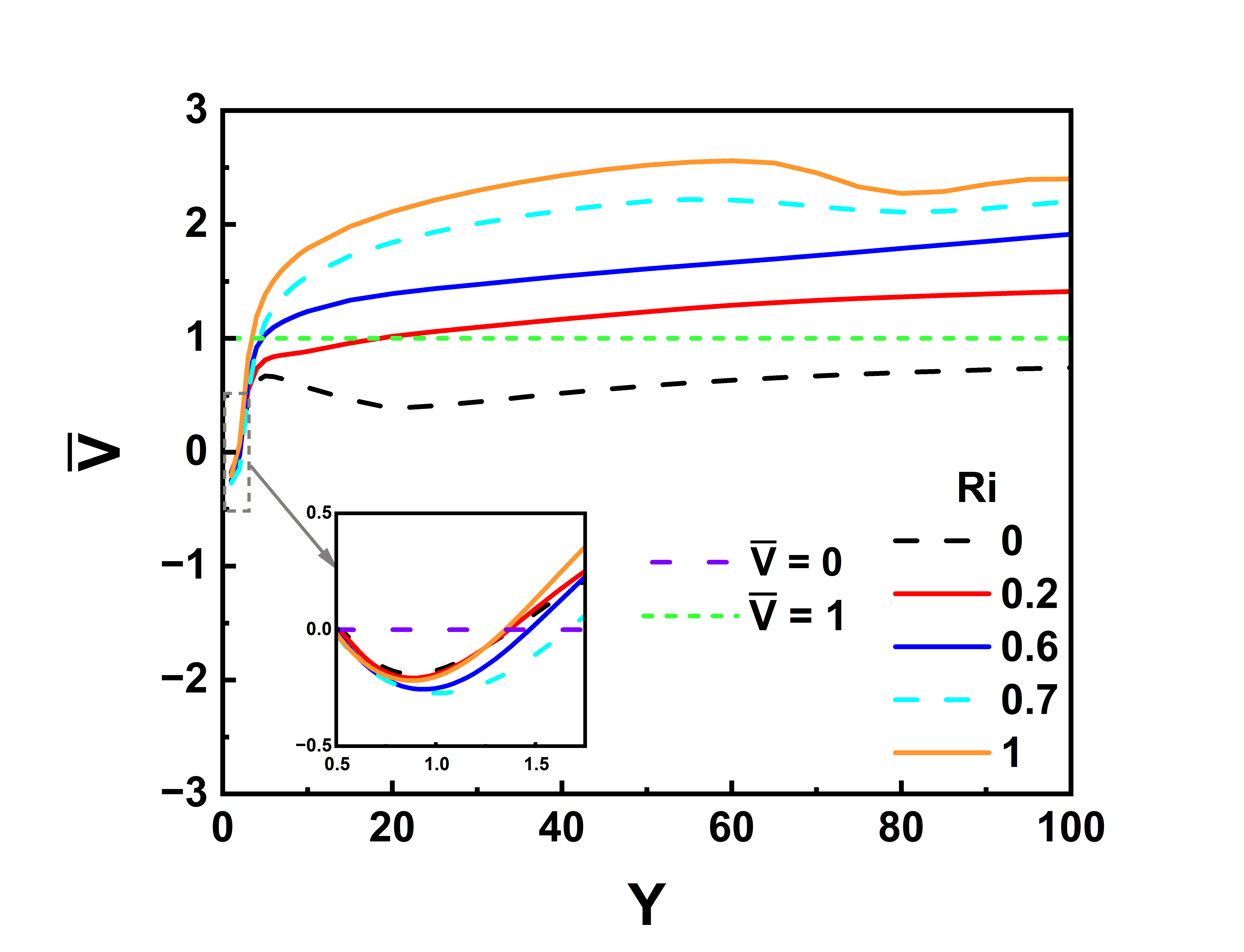
(a)

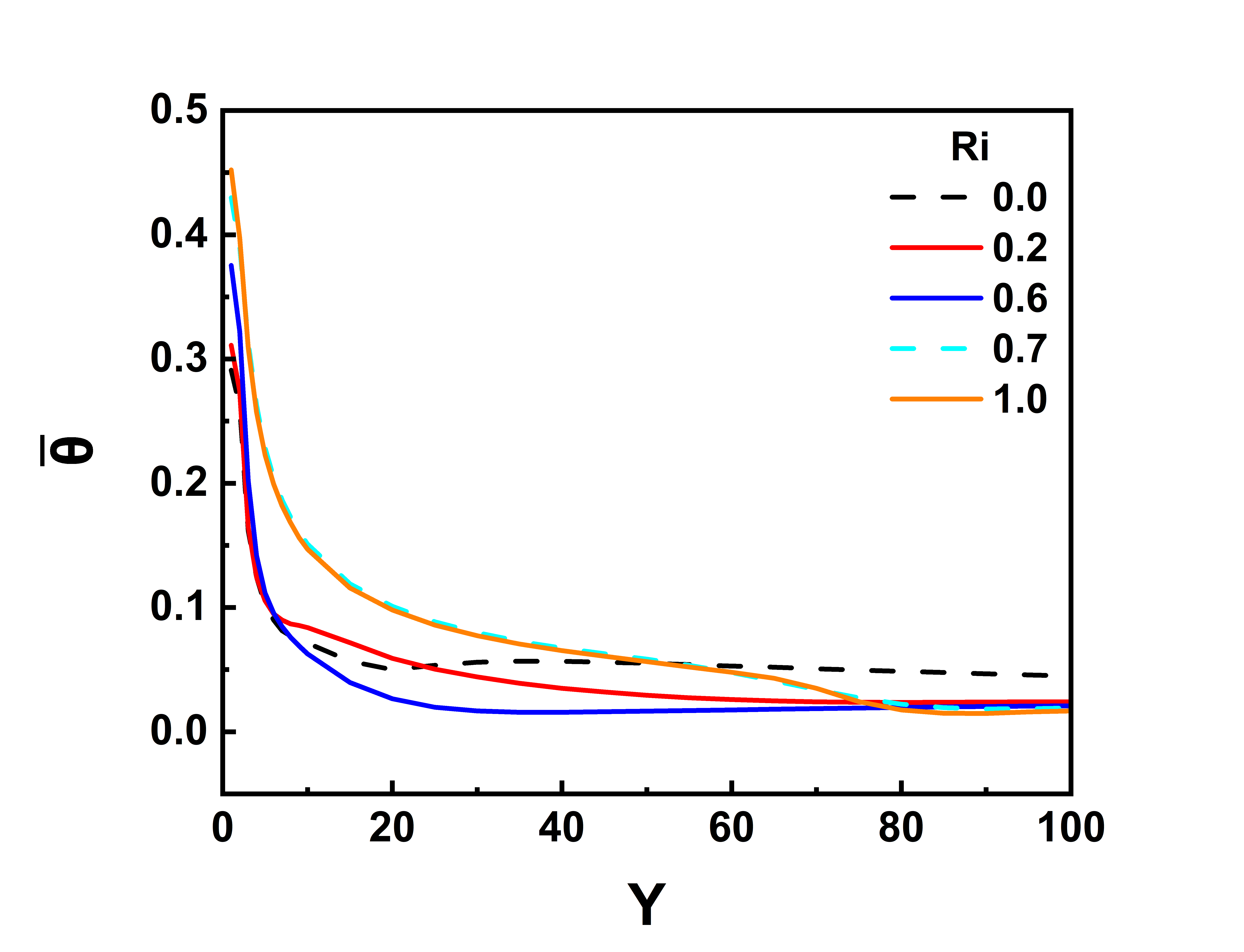
(b)

Figure 13: Variation of (a) centerline streamwise velocity and (b) centerline temperature.

Nusselt number is a function of the spatial coordinates as well as time. Therefore, it may be averaged in space, time, or both. $\overline{Nu}_{local}$ refers to the time-averaged local Nusselt number at a particular location on the cylinder, while $\overline{Nu}_{surface}$ refers to the temporally and spatially averaged Nusselt number for a particular surface on the cylinder, and $\overline{Nu}$ refers to the temporally and spatially averaged Nusselt number for the entire cylinder. Figure 14 shows the variation of time-averaged Nusselt number for different cylinder surfaces and local Nusselt number along the cylinder surface for various Ri, along with the nomenclature of the cylinder surfaces (AB-DA). For flow-facing surfaces (AB and DA), the mean Nusselt number increases with increasing Ri, whereas for wake-facing surfaces (BC and CD), the mean Nusselt number decreases with increasing Ri. There is a sharp decrease in the Nusselt number at Ri $=0.7$ for the wake-facing surfaces, and subsequently, in the Nusselt number for the full cylinder. The shedding phenomenon helps heat transfer by increasing mixing in the fluid by the mutual interaction of the two shear layers. When vortex shedding is suppressed, the momentum transport is inhibited as the mutual interaction of the shear layers is no longer active. Therefore, the Nusselt number sharply decreases for the wake-facing surfaces at Ri $=0.7$. The Nusselt number for the surfaces AB and DA, as well as that for surfaces BC and CD, are equal due to the symmetric nature of the time-averaged flow about the centerline. The local Nusselt number is the highest for the vertex A, which directly faces the forced flow, and it is considerably lower for the wake-facing surfaces compared to the flow-facing surfaces, due to the recirculation region having very weak streamwise velocities, causing decreased heat transfer from the wake-facing surfaces. The Nusselt number reaches a local maxima at the lateral corners of the cylinder (B and D), due to the acceleration of flow at these corners.

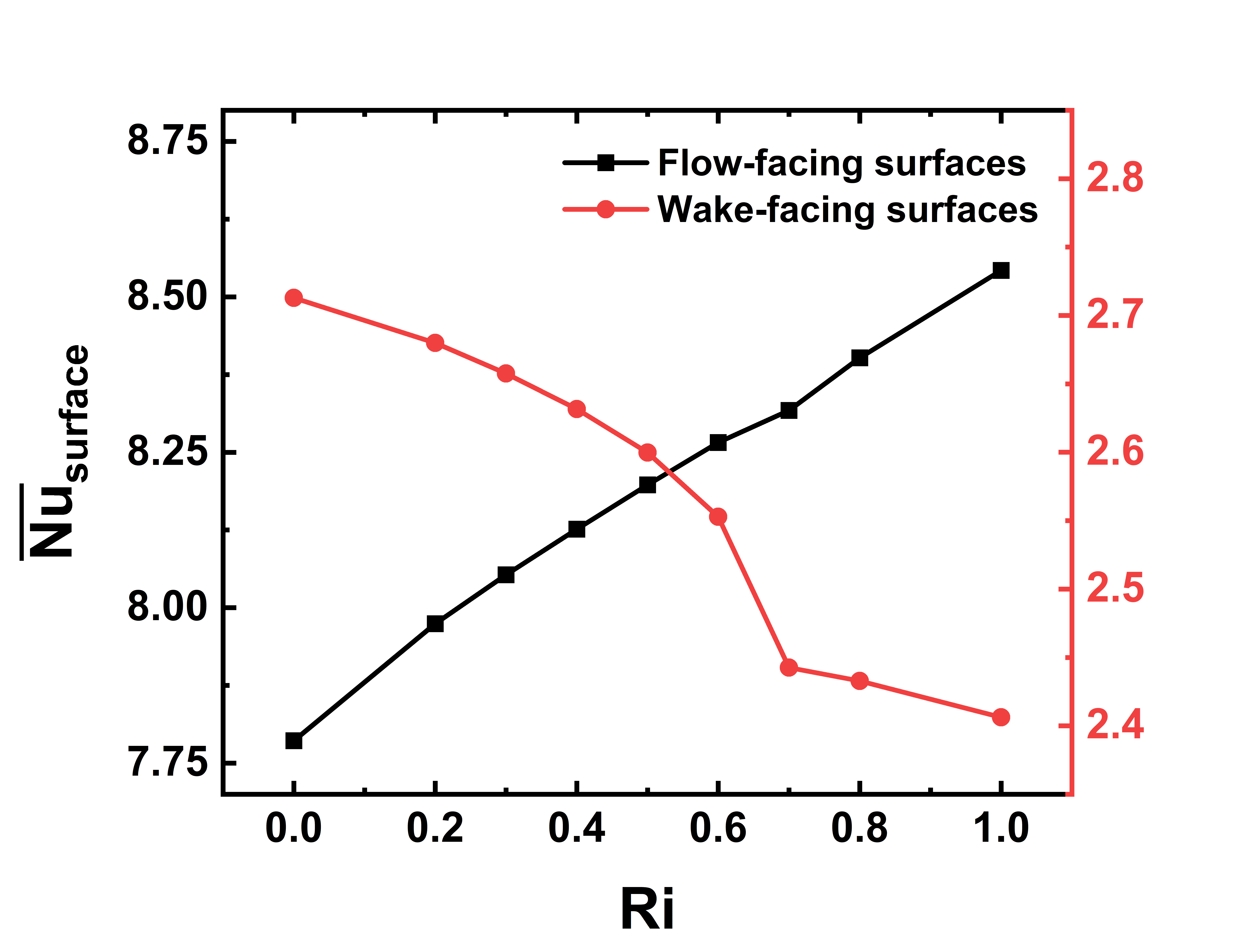
(a)

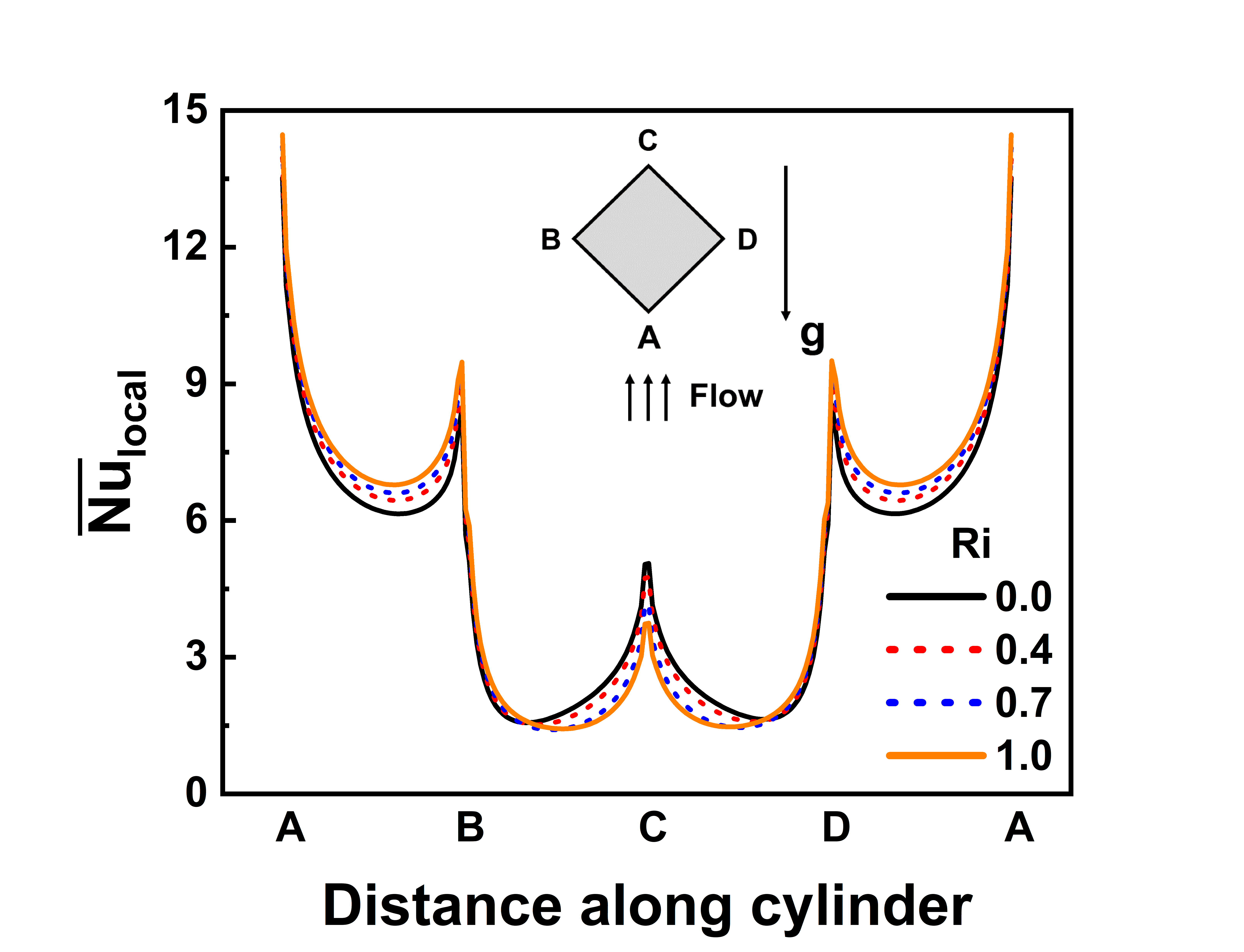
(b)

Figure 14: Variation of (a) time-averaged Nusselt number, and (b) local Nusselt number along the cylinder surface, for various Ri.

Table 8: Variation of force coefficients and Nusselt number with Richardson number (Ri).

Richardson number (Ri)	Drag coefficient ($C_{D}$)		RMS lift coefficient ($C_{L,\text{rms}}$)	Mean Nusselt number ($\overline{Nu}$)
	Mean ($\overline{C}_{D}$)	RMS ($C_{D,\text{rms}}$)
0.0	1.81	0.032	0.500	5.25
0.2	1.94	0.024	0.449	5.33
0.4	2.05	0.015	0.373	5.38
0.6	2.15	0.006	0.241	5.41
0.7	2.19	0.0	0.0	5.38
1.0	2.44	0.0	0.0	5.47

The variation of the integral parameters with Ri is shown in Table 8. $\overline{C}_{D}$ and $\overline{Nu}$ show an increase with increasing Ri. The buoyancy-driven flow in the vicinity of the cylinder increases both pressure drag and skin friction drag on the cylinder. On the other hand, as Ri increases, RMS quantities decrease. All quantities presented in Table 8 are near-field quantities, and hence, when the near-field is stabilized, these values become constant with no periodicity. Hence, RMS quantities fall to zero beyond the critical Ri. The RMS Nusselt number has not been reported as it is extremely small for all Ri. The mean Nusselt number presents an interesting variation. Below Ri $=0.7$, the Nusselt number increases monontonically, and it decreases to a local minimum value at Ri $=0.7$, and increases subsequently for Ri $>$ 0.7. Below 0.7, flow acceleration due to buoyancy forces causes thinning of the thermal boundary layer, leading to higher Nusselt numbers for the entire cylinder. There is a greater increase in the Nusselt number of the flow-facing surfaces compared to the decrease in the Nusselt number of the wake-facing surfaces, leading to an overall increase in the Nusselt number of the cylinder. However, at Ri $=0.7$, as discussed earlier, the Nu of the wake-facing surfaces sharply decreases due to the inhibition of vortex shedding, and this decrease is greater than the increase in the Nusselt number of flow-facing surfaces, leading to an overall decrease in the Nusselt number of the cylinder. Beyond Ri $=0.7$, an increase in cylinder Nu is seen, similar to the trend below Ri $=0.7$.

Figure 15 reveals the variation of recirculation and inversion lengths with Ri. For calculation of the inversion length, time-averaged vorticity data is taken for all streamwise locations at a transverse location X $=0.1$. The location of the first sign change in the vorticity data yields the inversion length. To ensure independence of the result from the choice of transverse location, we have also calculated inversion length using X $=0.2$, and the results reveal no variation based on the choice of X. For the calculation of recirculation length, time-averaged streamwise velocity data along the centerline is considered, and the location of the sign change in this data yields the recirculation length. There is a monotonic decrease in the inversion length up to Ri $=0.6$, followed by a slight increase at Ri $=0.7$ and a subsequent decrease for higher Ri. The decrease in inversion length is due to the increasing strength of the natural convective vorticity and the diminishing strength of the forced convective vorticity with increasing Ri. At low Ri, the forced convective component is strong, but it diminishes with downstream distance, while the natural convective component is weak in the near-field, but its strength grows with downstream distance. When Ri is increased, the strength of the natural convective vorticity closer to the cylinder also grows, as the buoyancy-driven flow transforms the entire flow field into a plume, while the wake behavior weakens. The recirculation length shows an interesting variation, which was discussed briefly with Figure 13(a). The recirculation length increases up to Ri $=0.7$ where it peaks, followed by a decrease. Prior to Ri $=0.7$, vortex shedding actively occurs in the flow. Due to the buoyancy, there is an inhibited interaction of the two shear layers as seen in near-field plots of vorticity and temperature (see Figures 4 and 6). This increases the shear layer length and consequently, the recirculation length, which increases up to Ri $=0.7$, where there is no vortex shedding and near-field flow becomes steady. Since the flow is steady, there is no mutual interaction between the opposite shear layers, which form a steady separation bubble, and the effect of increasing buoyancy is to cancel the vorticity caused by the forced convective part, which reduces the length of the separation bubble.

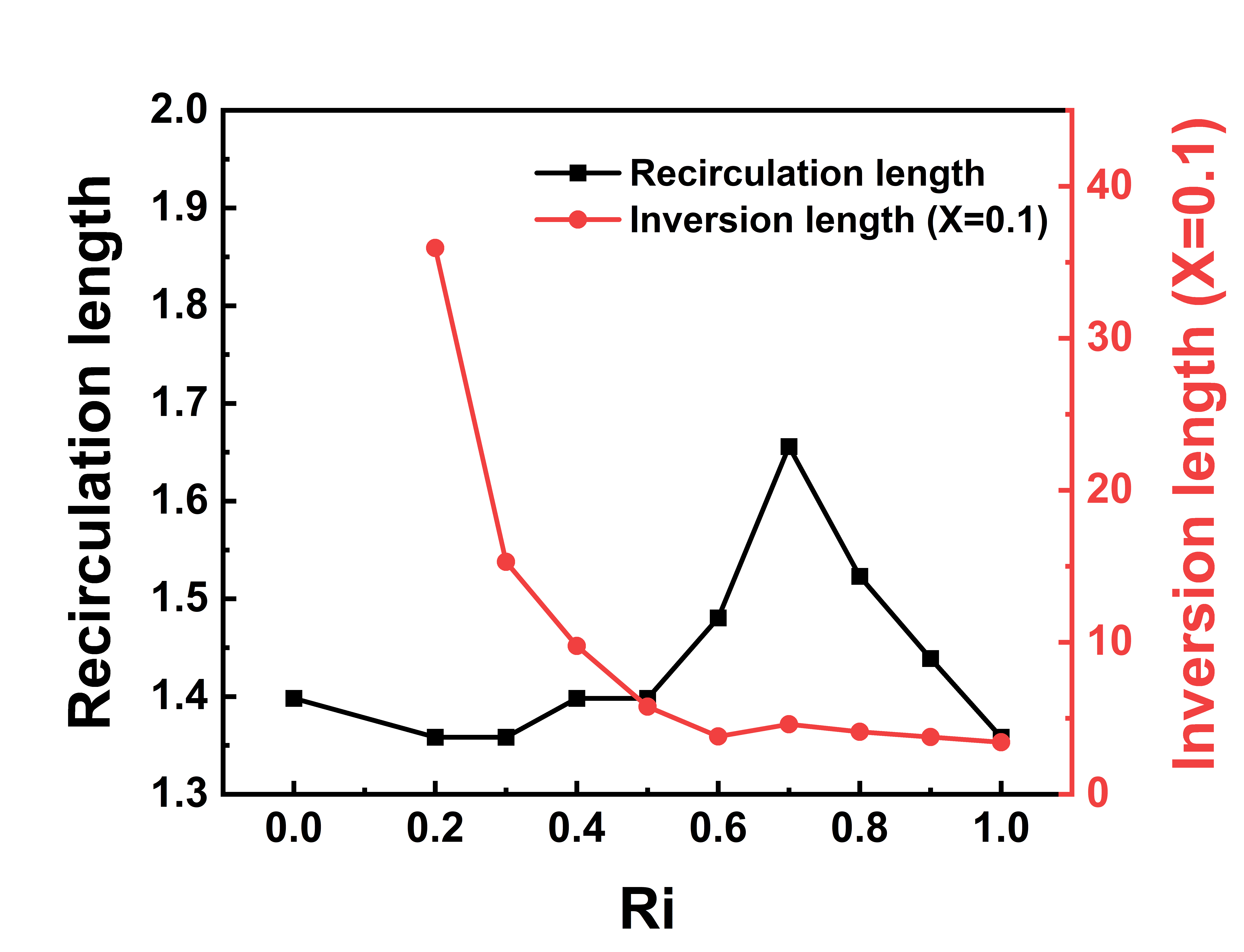
Figure 15: Variation of recirculation and inversion lengths with Richardson number. Recirculation length has been calculated by considering the time-averaged centerline (X $=0$) velocities, while the inversion length has been calculated by considering time-averaged velocities parallel to the centerline at X $=0.1$.

Streamwise velocity, transverse velocity, vorticity, and temperature profiles at different streamwise locations for different Ri are shown in Figures 16, 17, 18 and 19, respectively. Figure 16 shows the deficit of momentum in the near-field associated with wake-like behavior and a recovery and subsequent excess of momentum in the intermediate and far-fields. In the near-field, the deficit of momentum is seen for all Ri, resembling the profile seen in wakes. With increased downstream distance, the recovery of momentum occurs, starting earlier downstream for higher Ri, followed by lower Ri later downstream. At Y $=30$, the recovery of momentum is complete for all positive Ri, and there is an excess of momentum seen for higher Ri, which grows more pronounced further downstream, resembling the profile seen in jets. Therefore, the flow field downstream starts out as that of a wake at low Ri and slowly transforms into that of a plume as Ri is increased, first far downstream, then near the cylinder as well. Such behavior is attributed to the buoyancy-driven flow, whose tendency is to cause a jetting effect in the complete flow field, starting from the far downstream region and slowly coming towards the cylinder. Figure 17 shows the variation of transverse velocity, which is positive in the left half and negative in the right half of the flow for all positive Ri at all downstream locations. Figure 18 reveals the inversion of vorticity in the near and intermediate fields. For higher Ri, the inversion occurs earlier downstream, while for lower Ri, it occurs further downstream as the strength of the natural convective vorticity is lesser at lower Ri. The peak vorticity is seen to be higher for higher Ri. Figure 19 shows the temperature profiles for different streamwise locations. Overall, the temperature shows a dissipating trend with increased streamwise distance. We also observe that prior to the onset distance of the far-field unsteadiness, the temperature profile width for the cases above the critical Ri is much lower than that of the cases below the critical Ri (see Figure 19(e)). However, after the onset distance of the far-field unsteadiness, the profile widens drastically, and it is comparable with the cases below the critical Ri (see Figure 19(f)).

The inversion of vorticity has been reported in the literature for isothermal confined flows [13, 14, 15, 16]. The interplay between several sources of vorticity in the flow causes the reversal of vorticity in the wake of the cylinder. In unconfined flows, a reversal of the Bénard-von Kármán vortex street takes place when the obstacle (bluff body or aerofoil) is imparted a periodic motion. Under appropriate conditions of the shape of the body or the control parameter, the shed vortices cross the centerline and switch their position after traveling downstream, which manifests as a jet profile with a momentum excess in the time-averaged velocity plot, compared to the original wake profile with a momentum deficit [40, 41, 42]. We have seen similar behavior in the flow structures obtained for our case (see Figure 3), however, the shed vortices do not physically convect to the opposite side in our case. Rather, there is an inversion of vorticity due to the interplay between the forced convective and natural convective vorticity, as discussed earlier.

The forced convective component of the flow causes shear layer separation at the downstream corners of the cylinder, causing a deficit of momentum in the wake. On the other hand, the natural convective component causes jet-like behavior downstream, competing with the deficit caused by the wake, with the respective vorticities signed oppositely to each other. The opposing effects of these two flow components lead to a vorticity inversion. This inversion does not occur for Ri $=0.0$ due to the absence of the buoyancy-driven flow at this Ri. For positive Ri, vorticity inversion occurs downstream at an inception point, which comes further upstream as Ri is increased (see Figure 15), due to the increased buoyancy (see Figures 3 and 9). Prior to the reversal of vorticity, the downstream region has a wake-like behavior with a momentum deficit, and beyond the reversal of vorticity, the dowstream region exhibits a plume-like behavior, with momentum excess seen in the time-averaged velocity profile (see Figure 16). The strength of the wake decreases with increased downstream distance, while the plume shows the opposite behavior. Such behavior resembles that of fish-like swimming and flapping foil propulsion in the time-averaged sense, but not in the instantaneous sense, because the shed vortices do not physically travel to the opposite side in our case. Instead, the greater strength of the natural convective vorticity causes the change of sign of vorticity on either side of the centerline by dominating over the forced convective vorticity, whose strength diminishes with increased downstream distance. The far-field unsteadiness also shows characteristics dissimilar to flapping foil cases, in that there are no discrete vortices in the far-field of the present case. The shear layers that were already shed in the near-field suddenly undergo large-scale undulation in the far-field, which appears to be due to the pronounced strength of the natural convective jet.

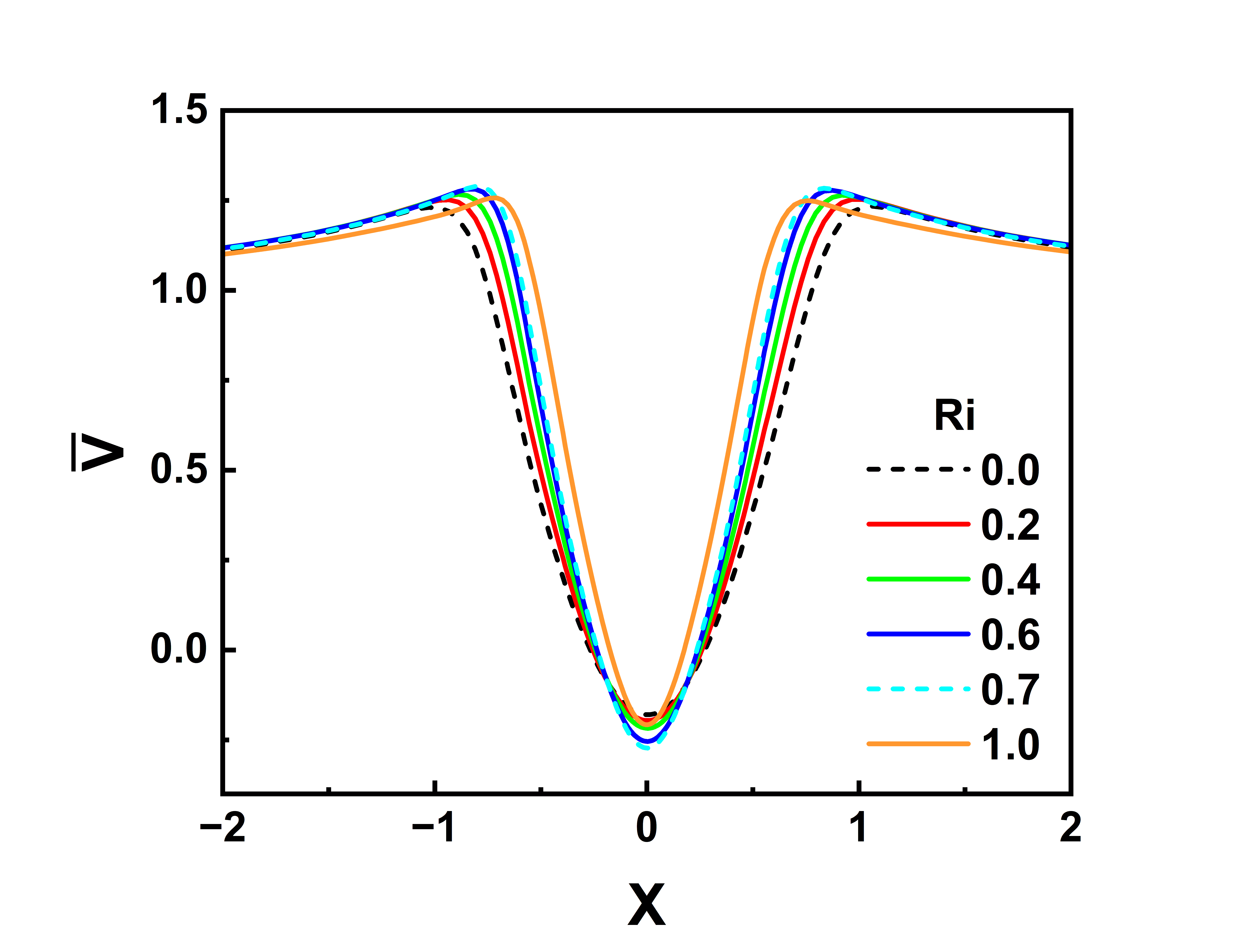
(a) Y $=1$

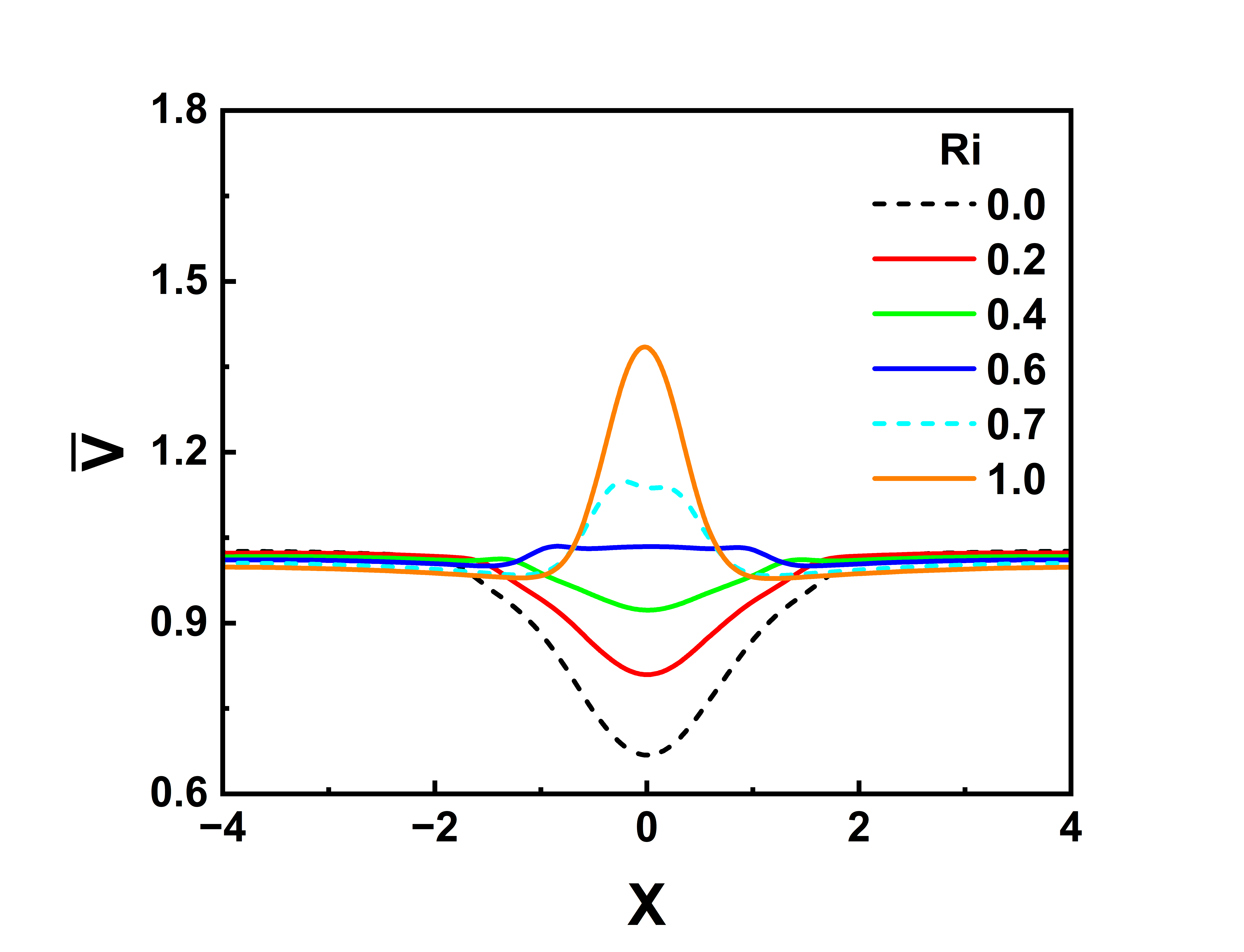
(b) Y $=5$

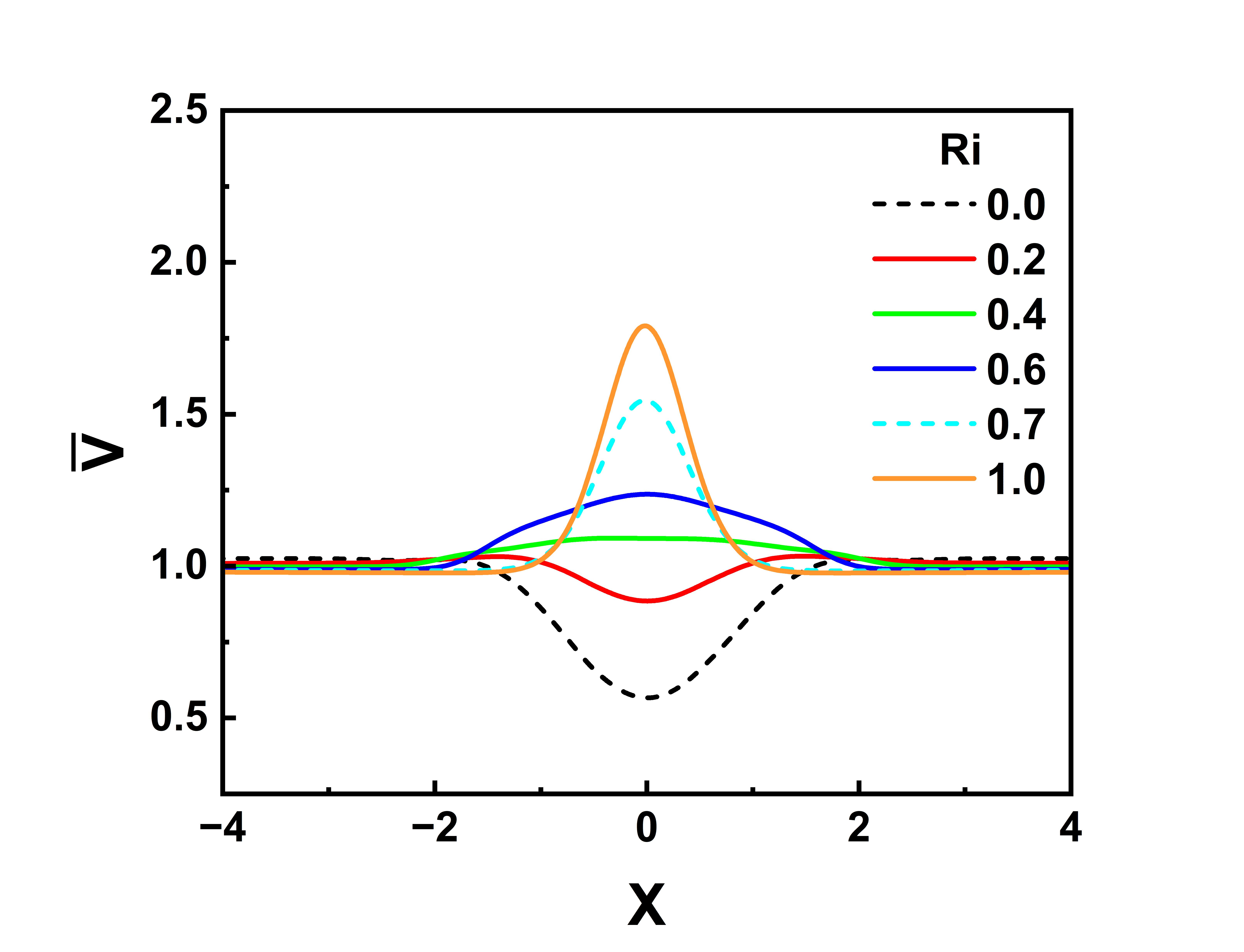
(c) Y $=10$

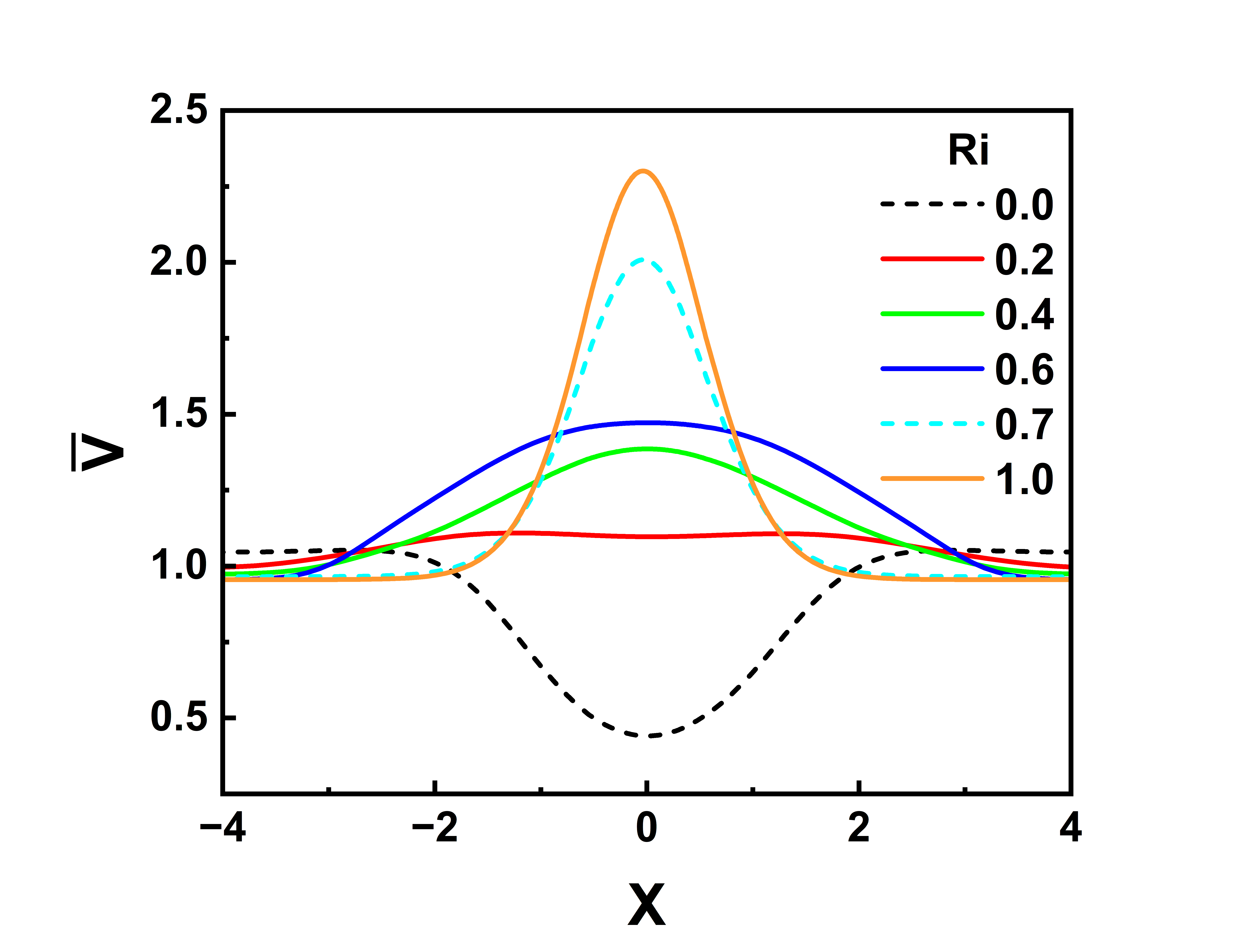
(d) Y $=30$

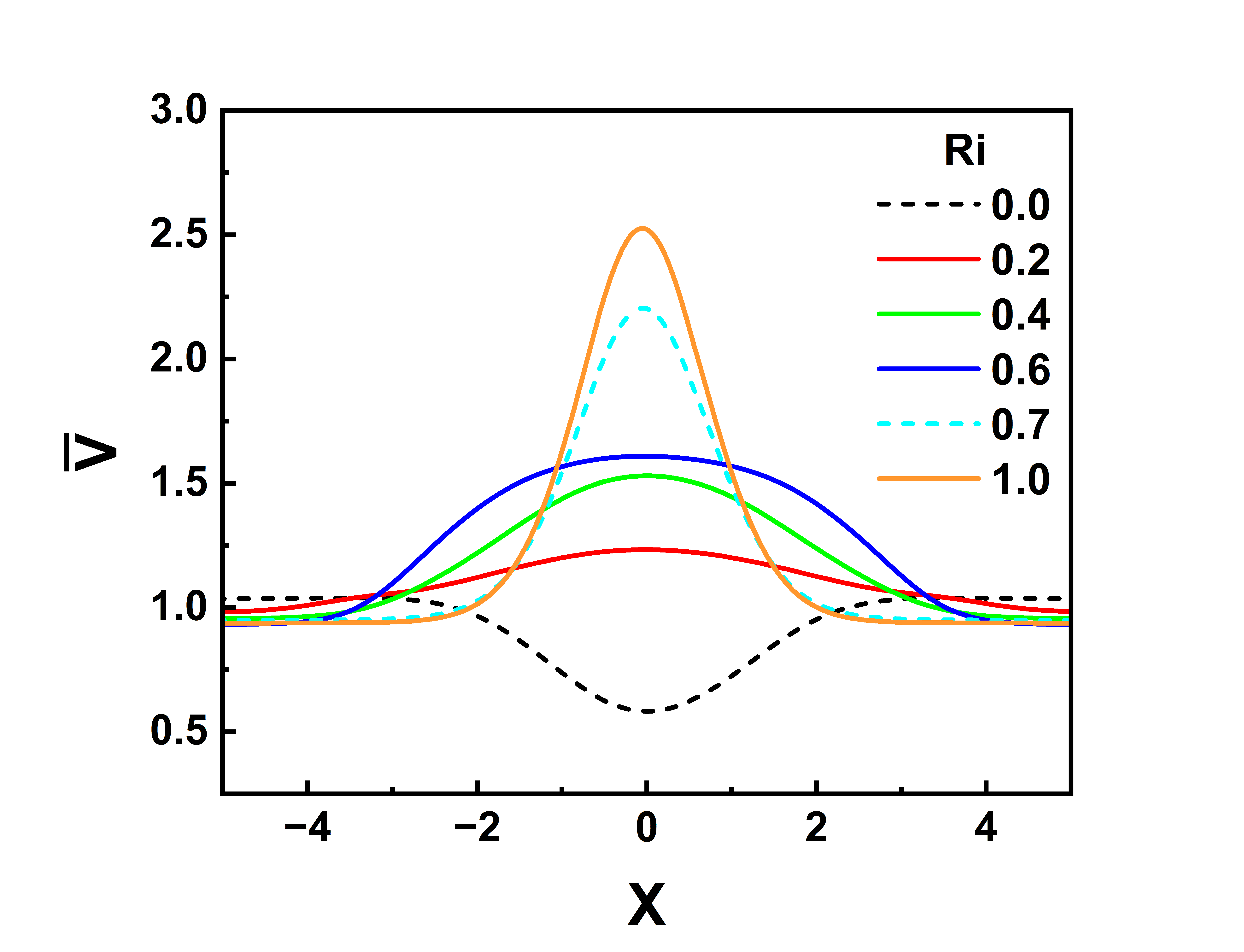
(e) Y $=50$

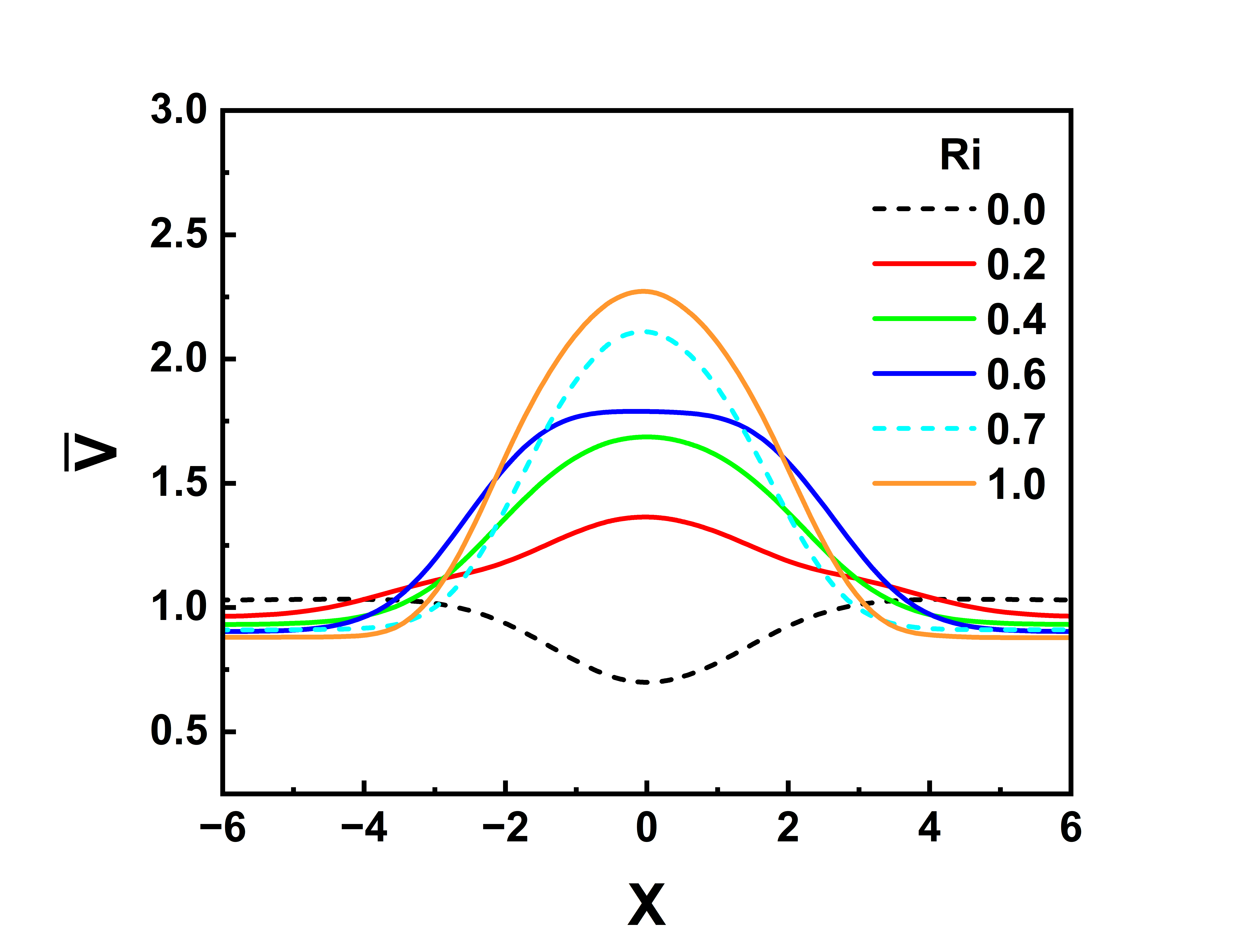
(f) Y $=80$

Figure 16: Streamwise velocity profile at (a) Y $=1$, (b) Y $=5$, (c) Y $=10$, (d) Y $=30$, (e) Y $=50$, and (f) Y $=80$.

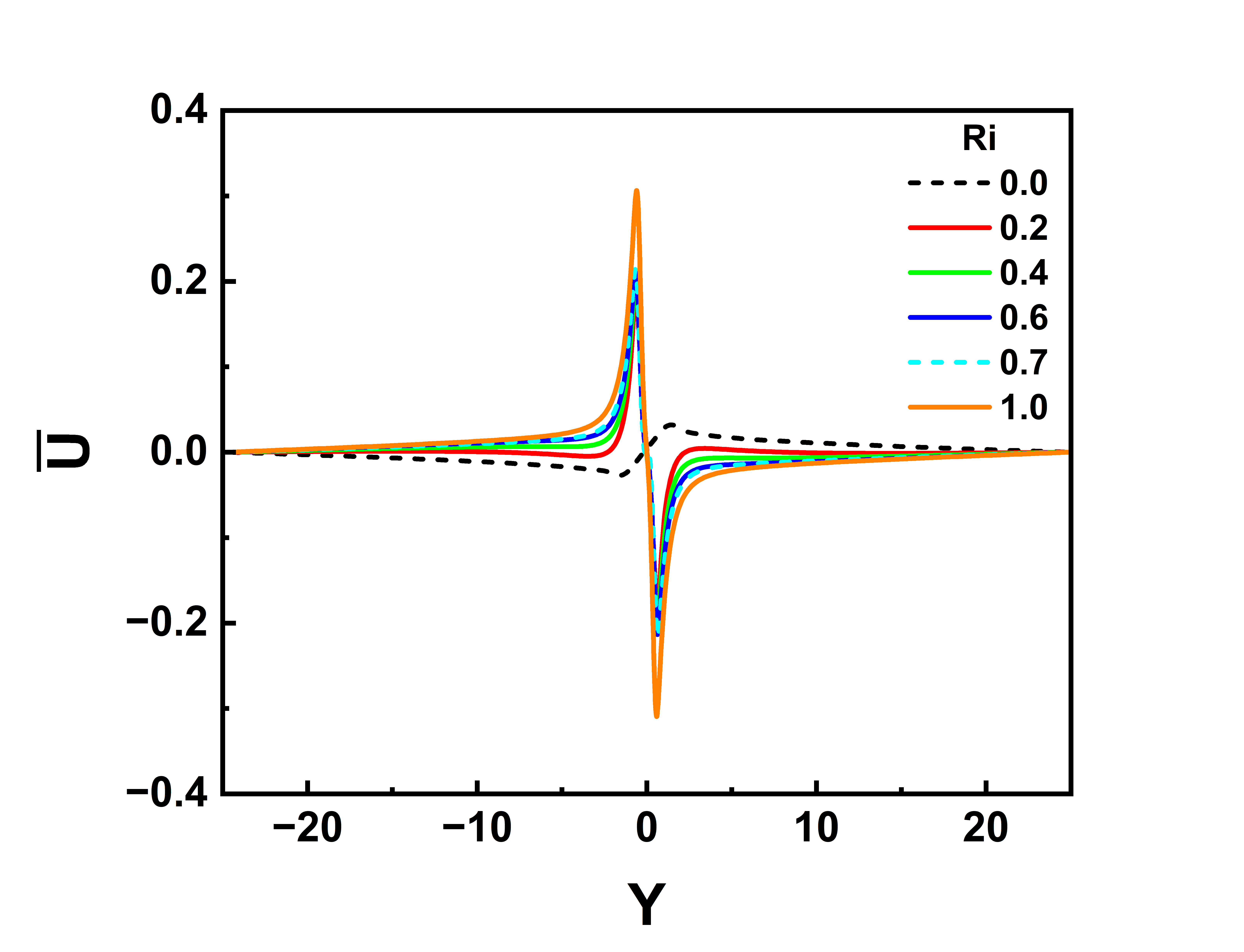
(a) Y $=1$

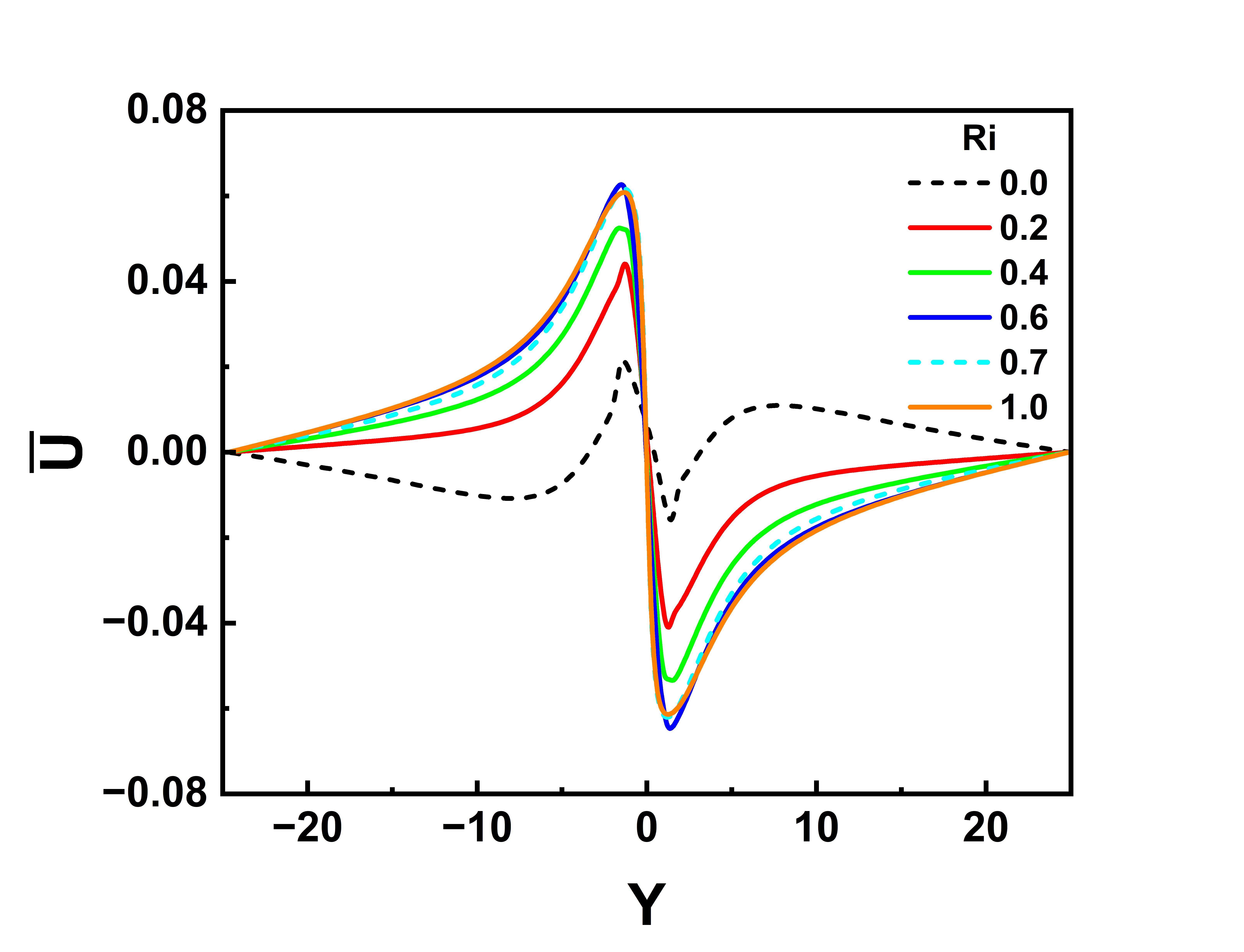
(b) Y $=5$

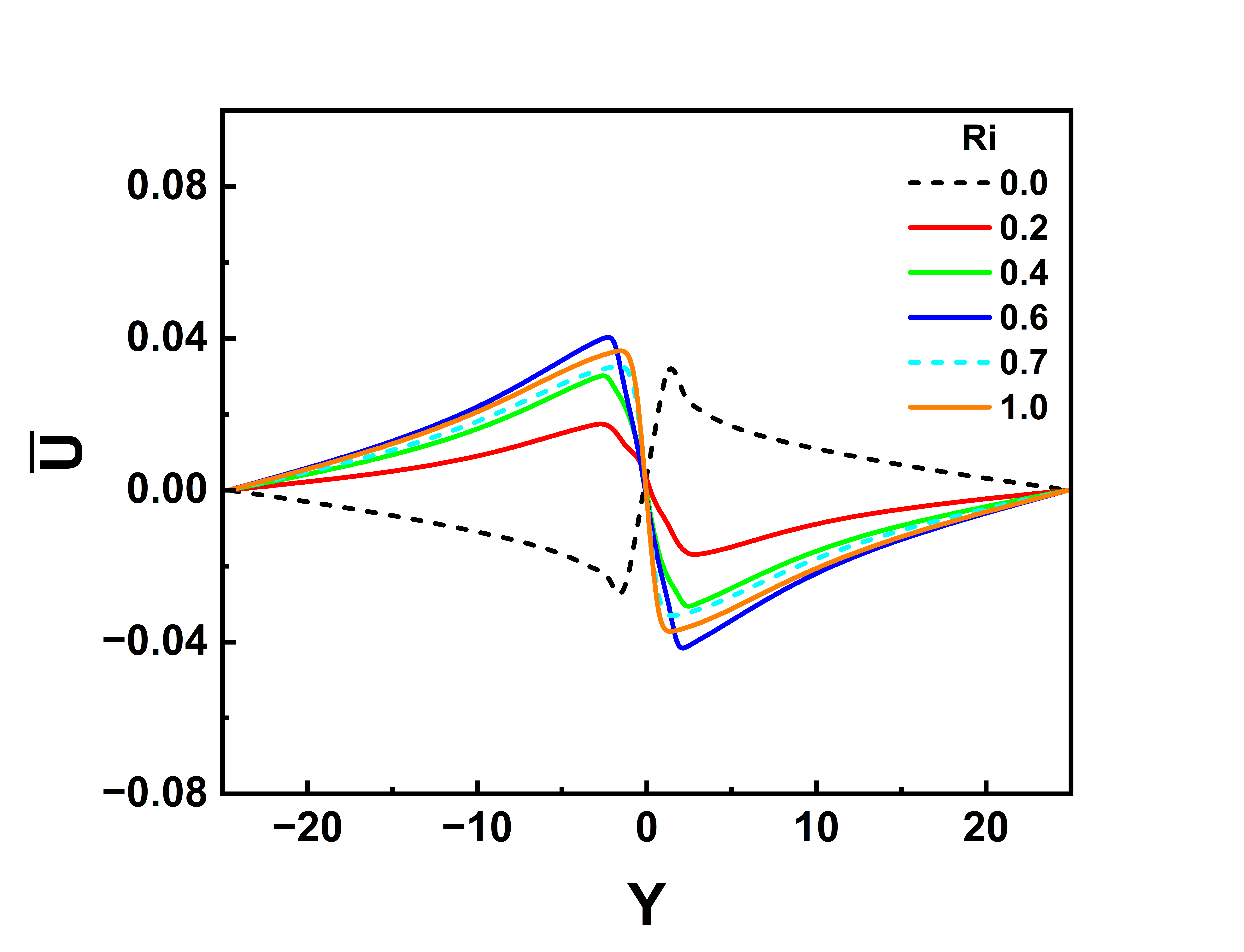
(c) Y $=10$

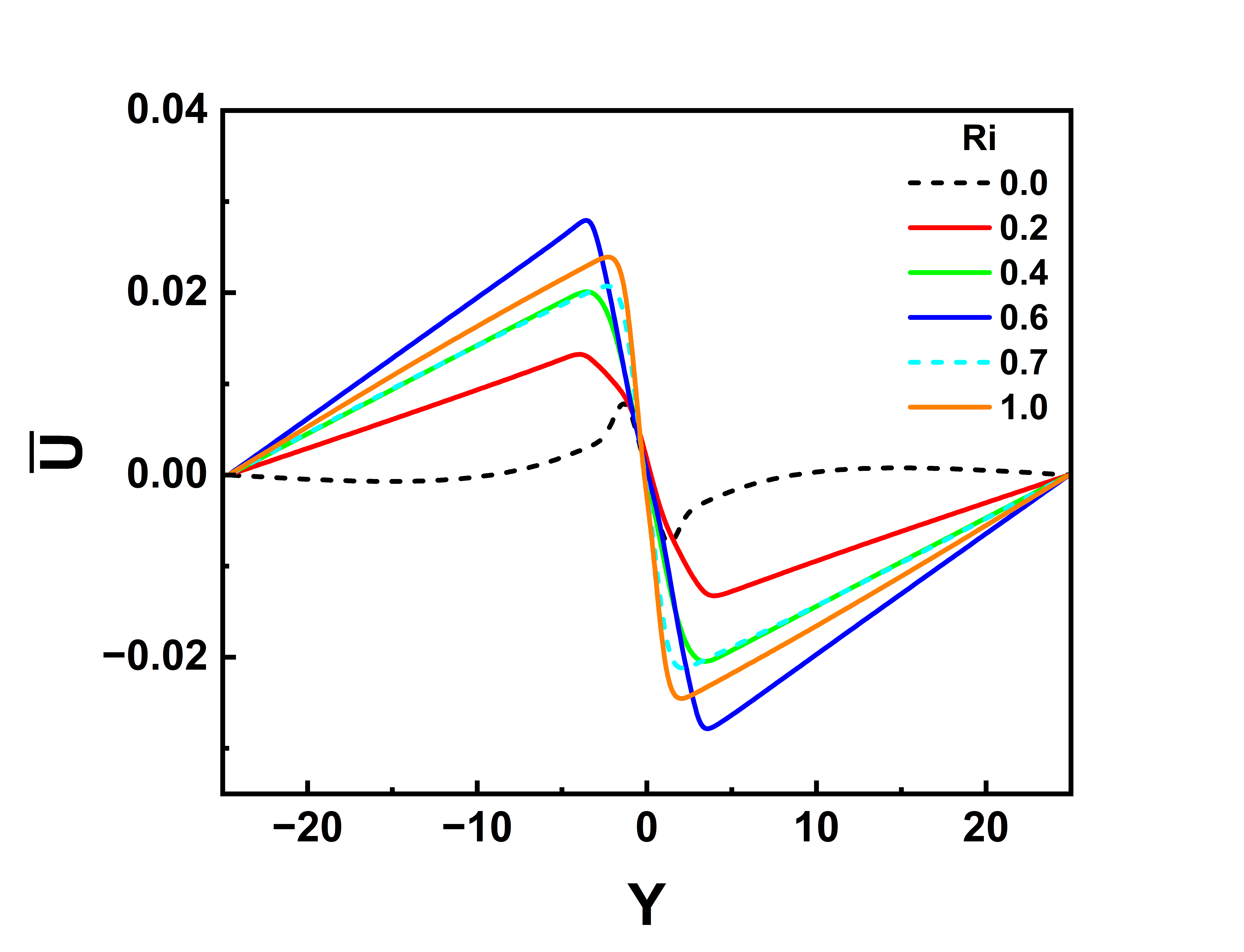
(d) Y $=30$

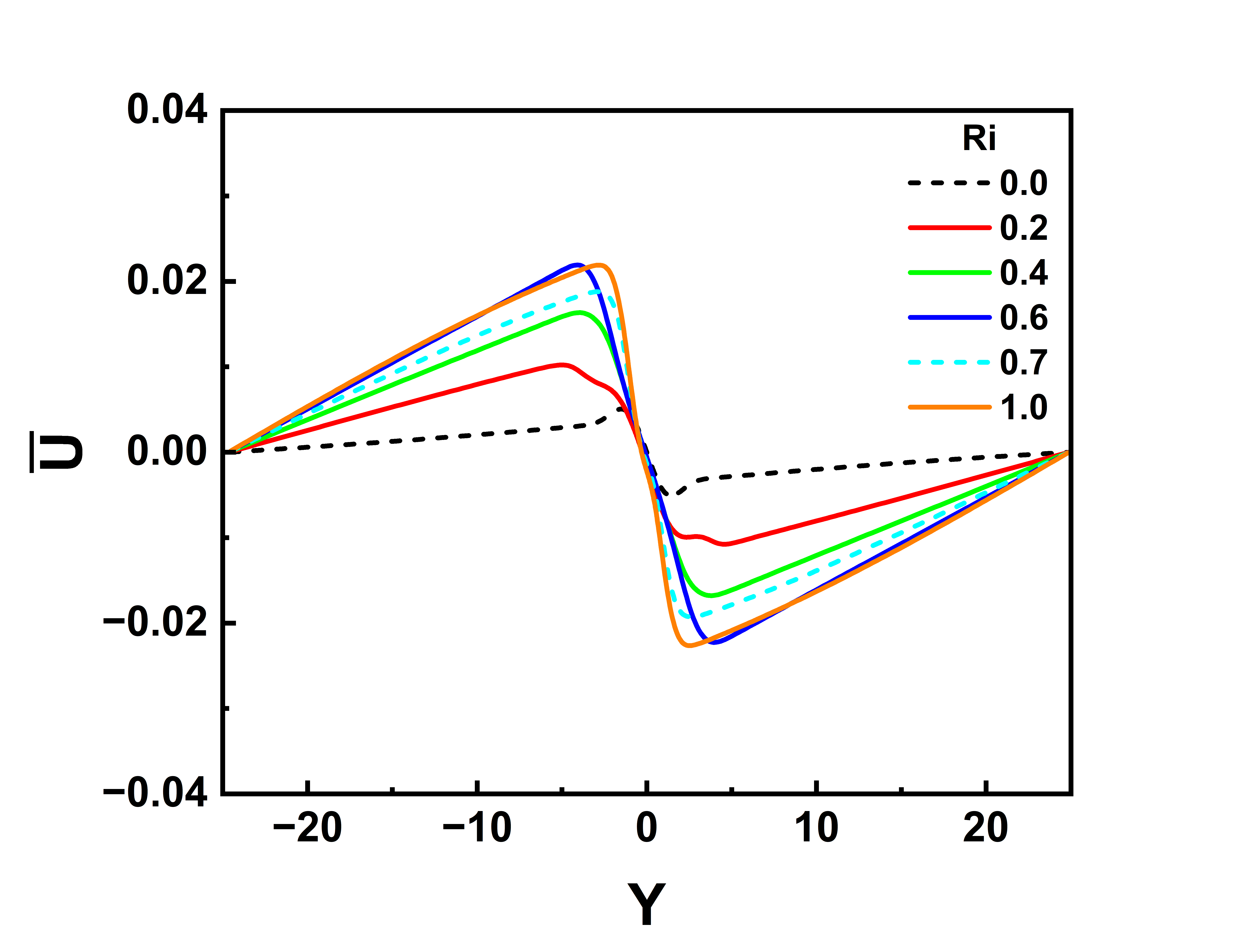
(e) Y $=50$

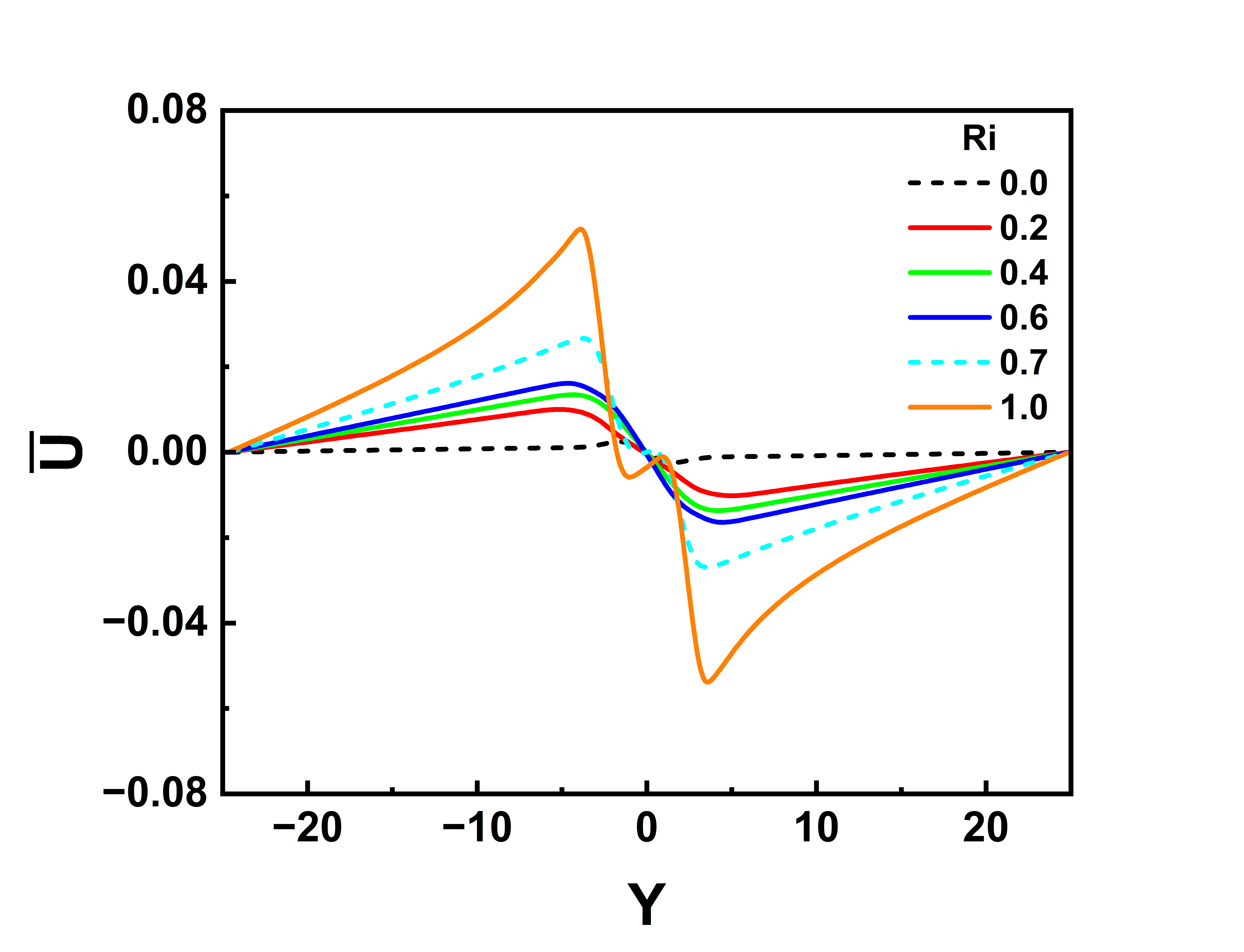
(f) Y $=80$

Figure 17: Transverse velocity profile at (a) Y $=1$, (b) Y $=5$, (c) Y $=10$, (d) Y $=30$, (e) Y $=50$, and (f) Y $=80$.

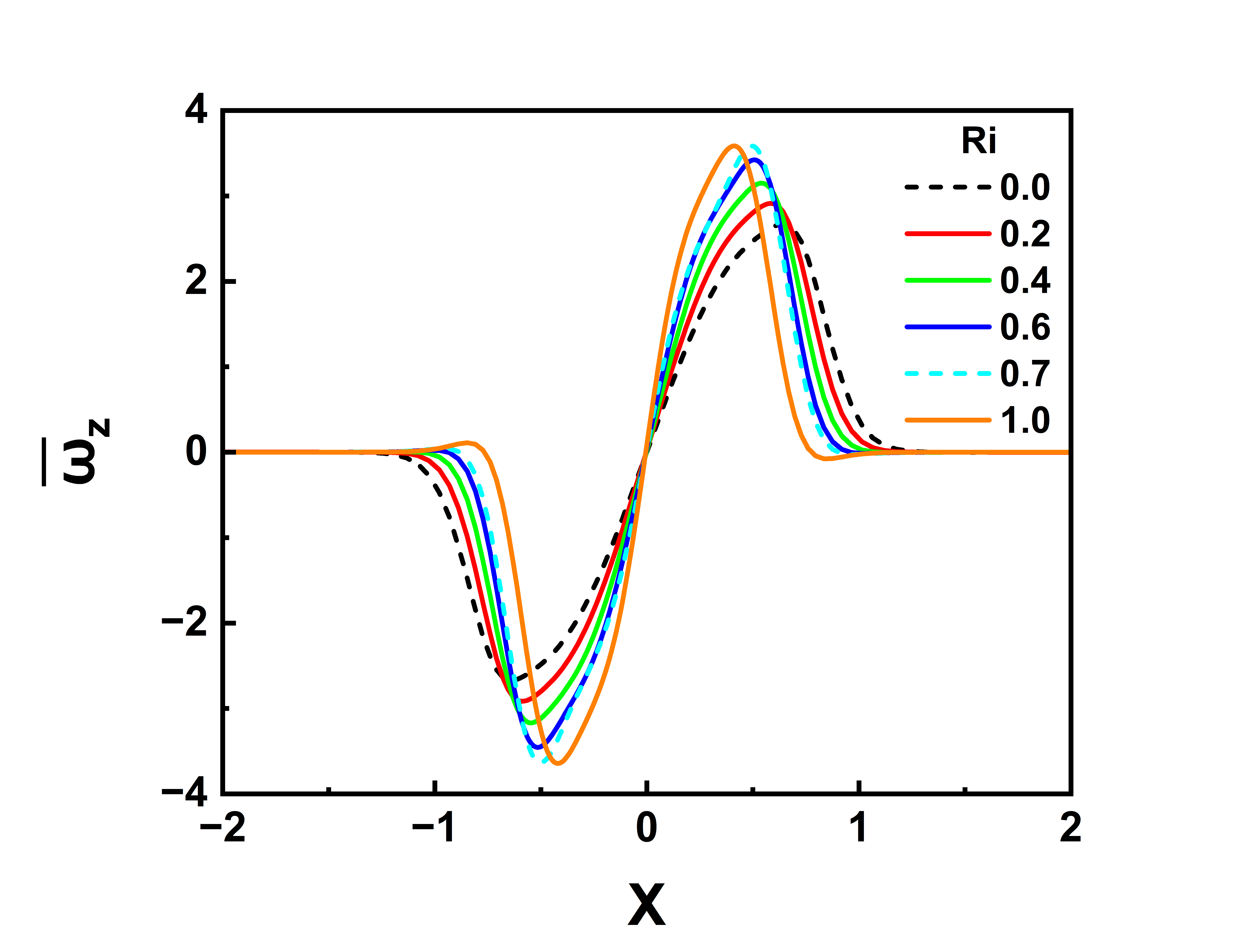
(a) Y $=1$

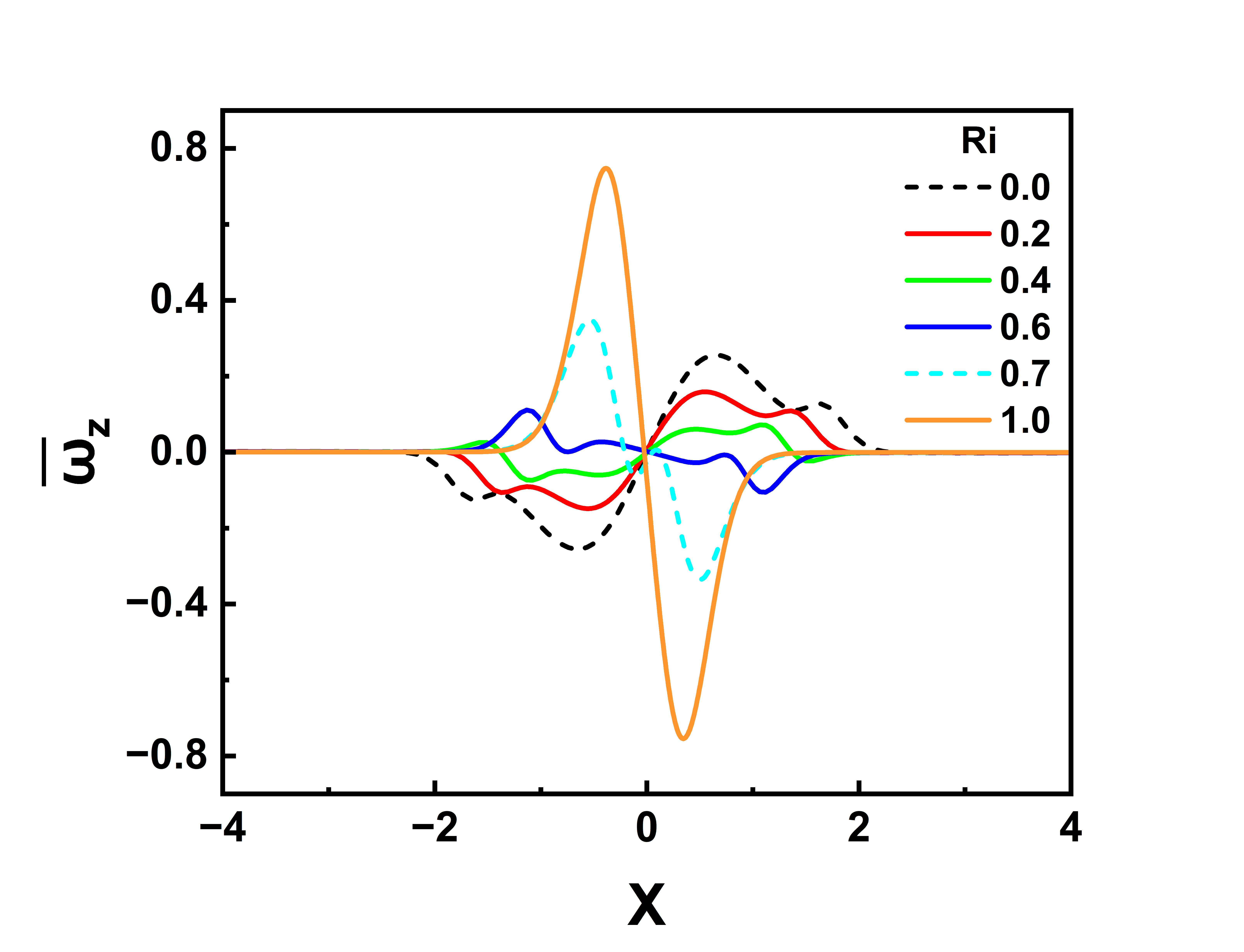
(b) Y $=5$

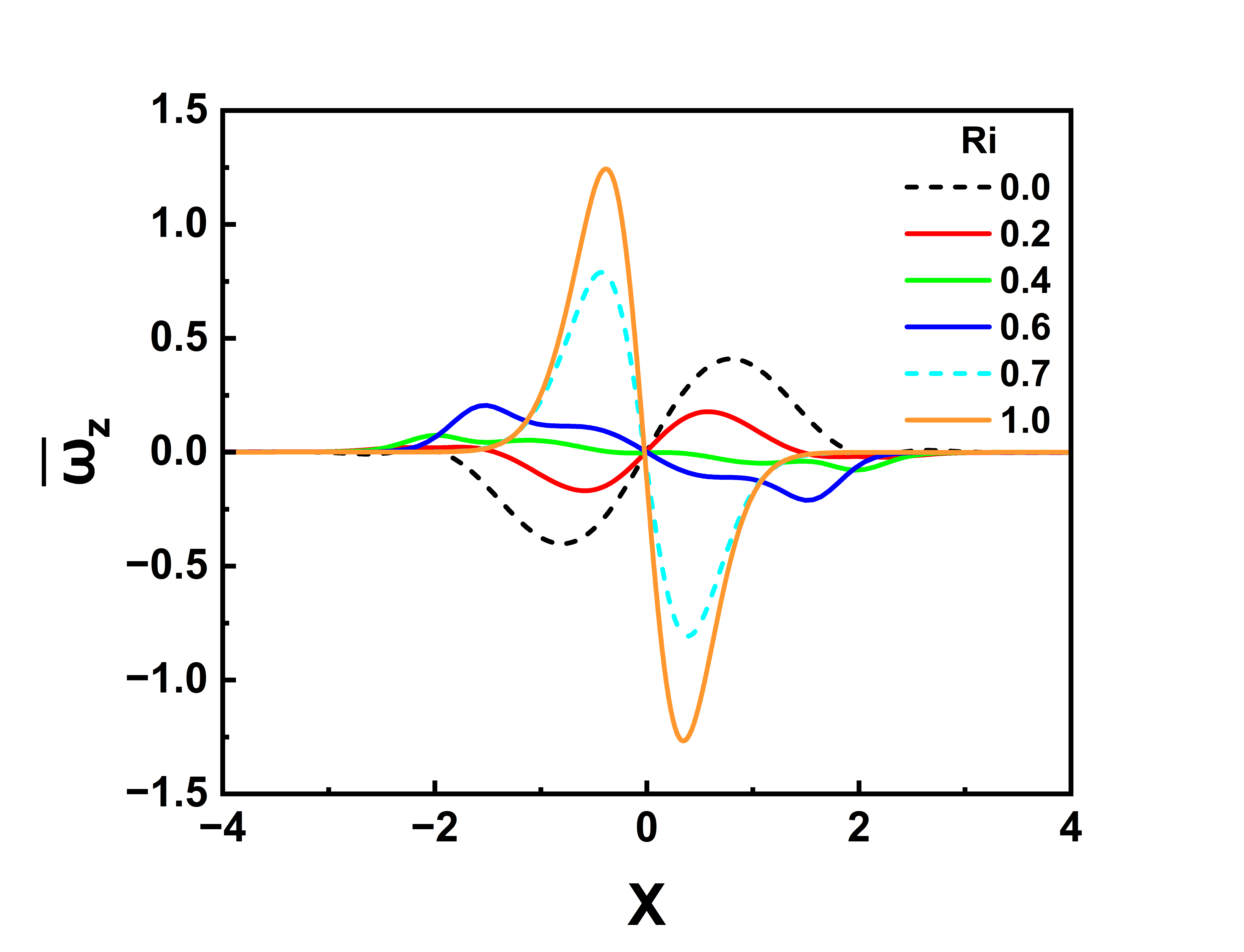
(c) Y $=10$

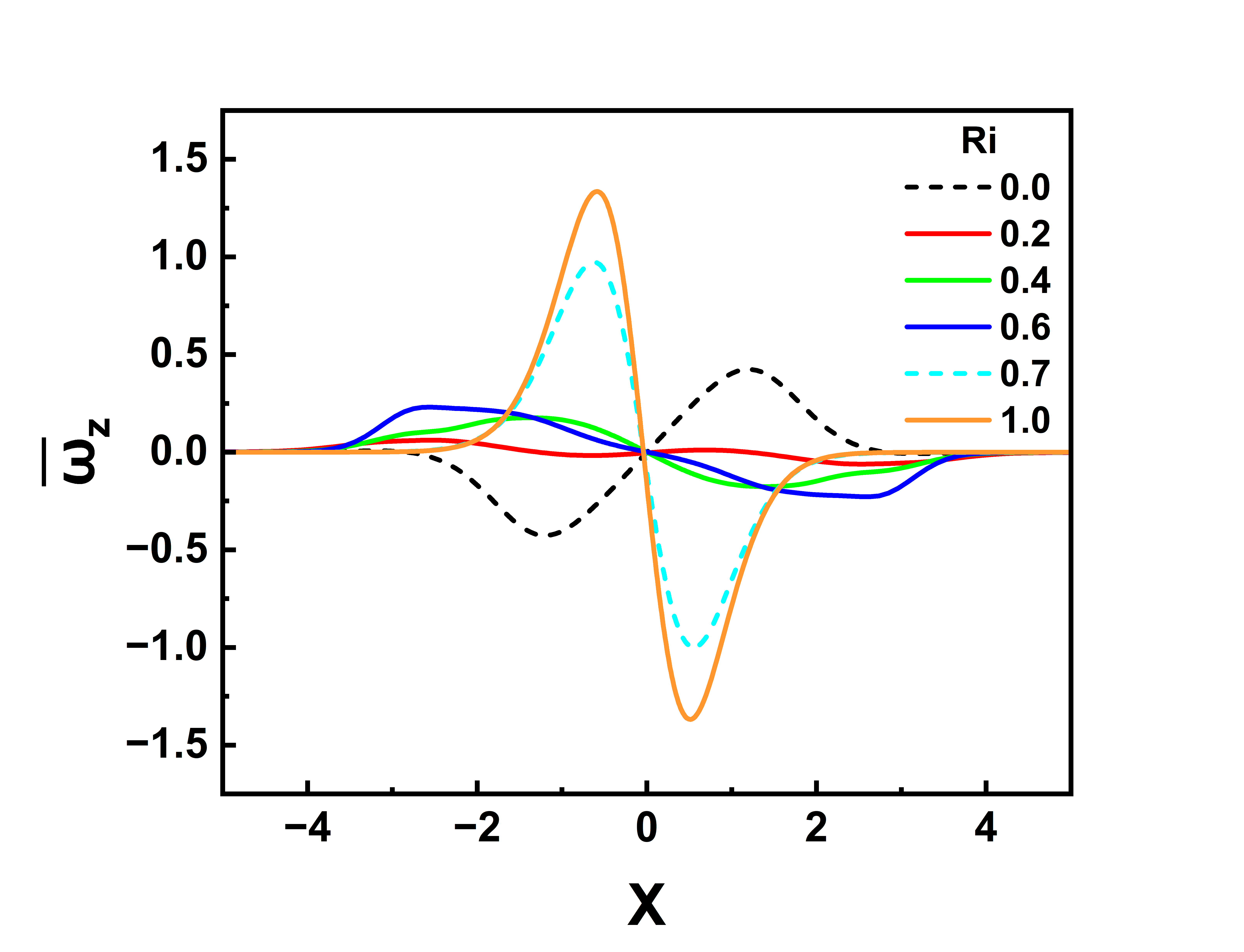
(d) Y $=30$

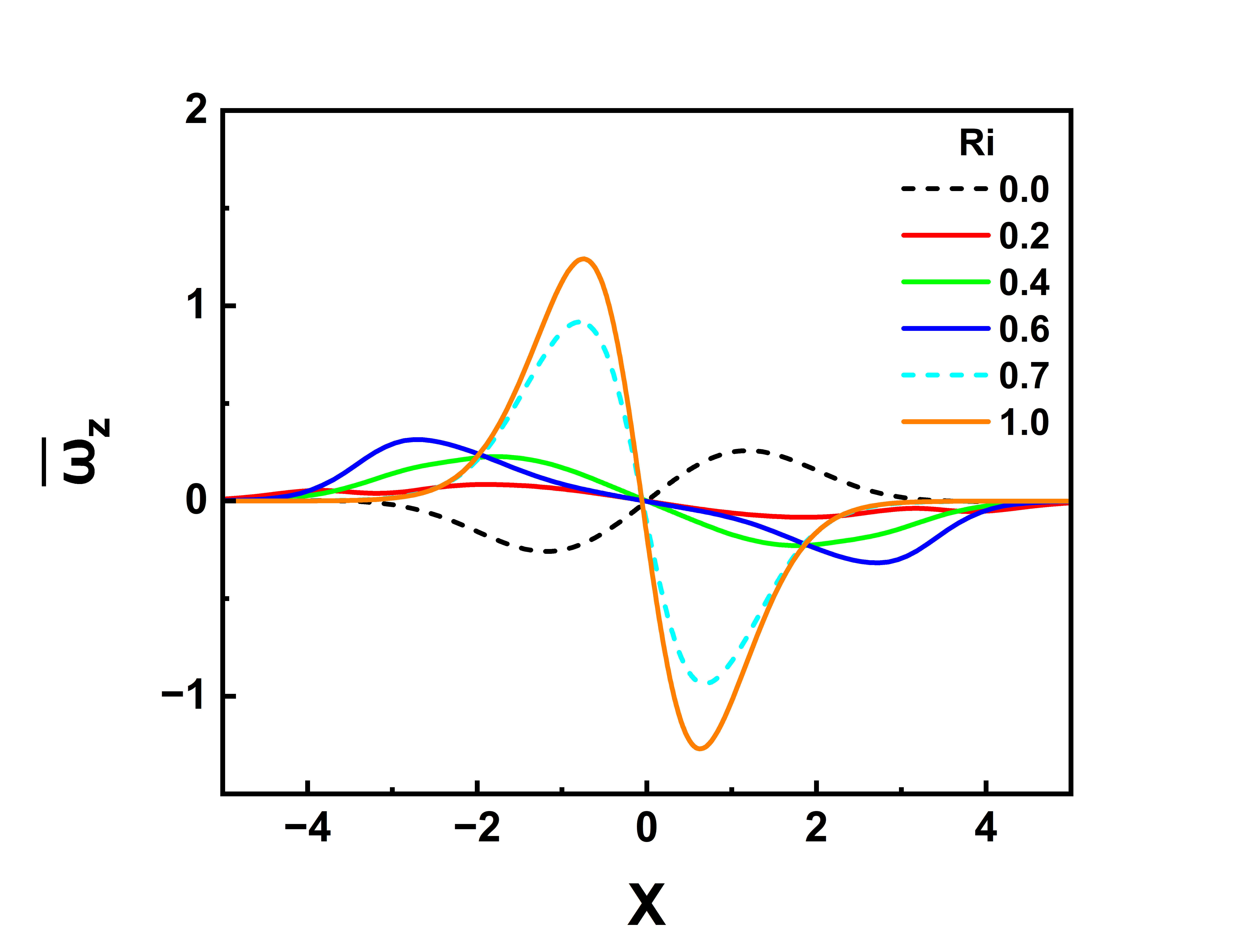
(e) Y $=50$

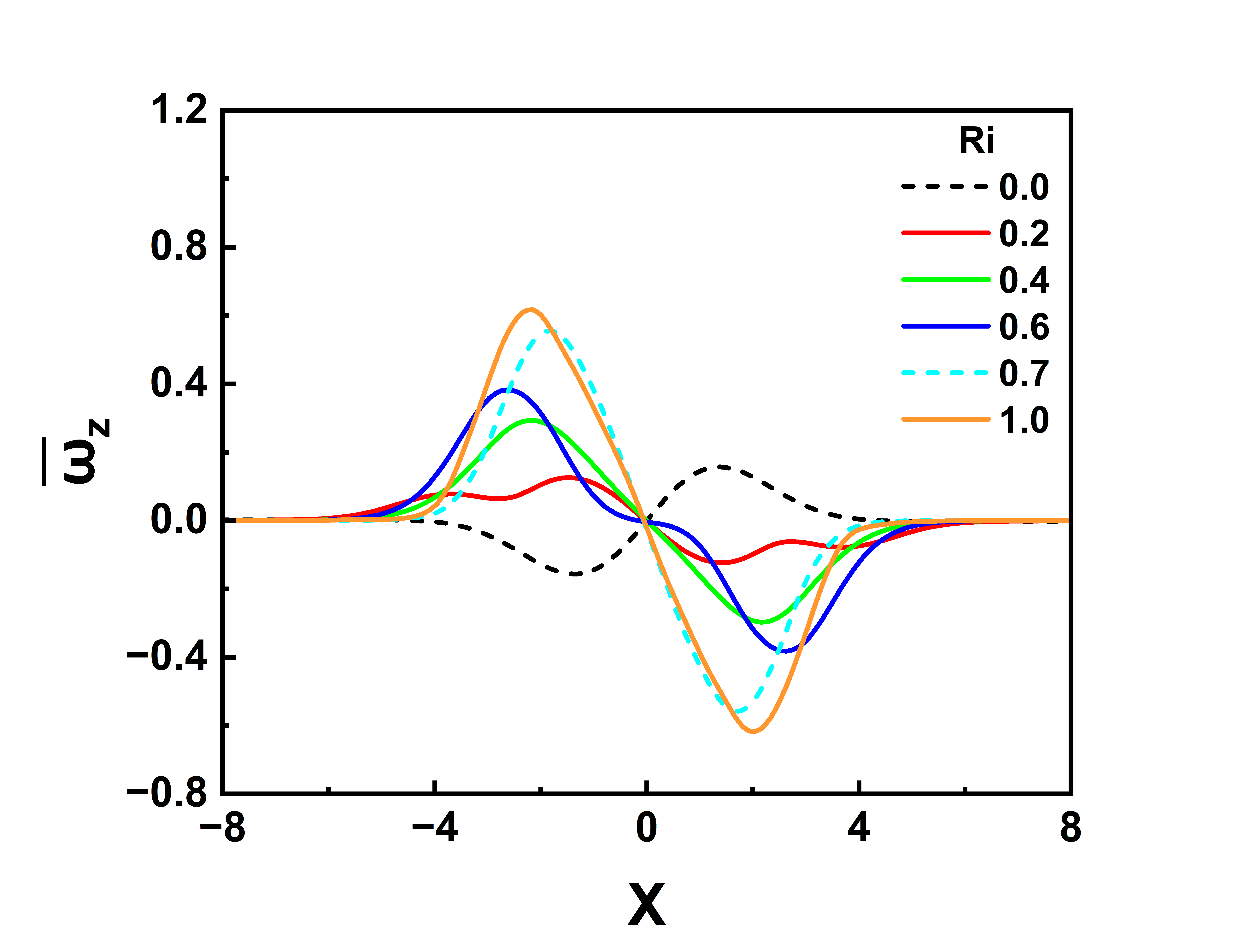
(f) Y $=80$

Figure 18: Vorticity profile at (a) Y $=1$, (b) Y $=5$, (c) Y $=10$, (d) Y $=30$, (e) Y $=50$, and (f) Y $=80$.

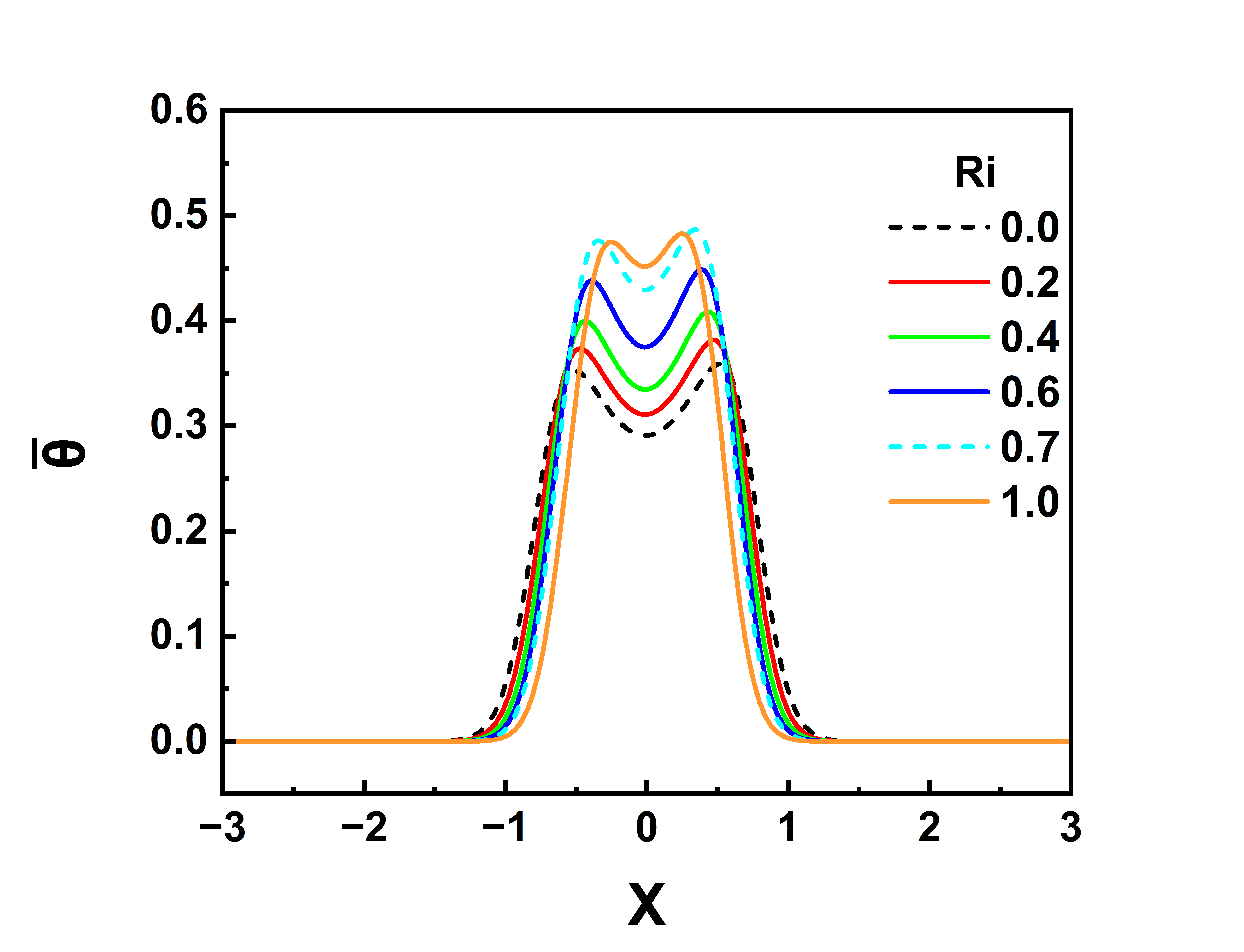
(a) Y $=1$

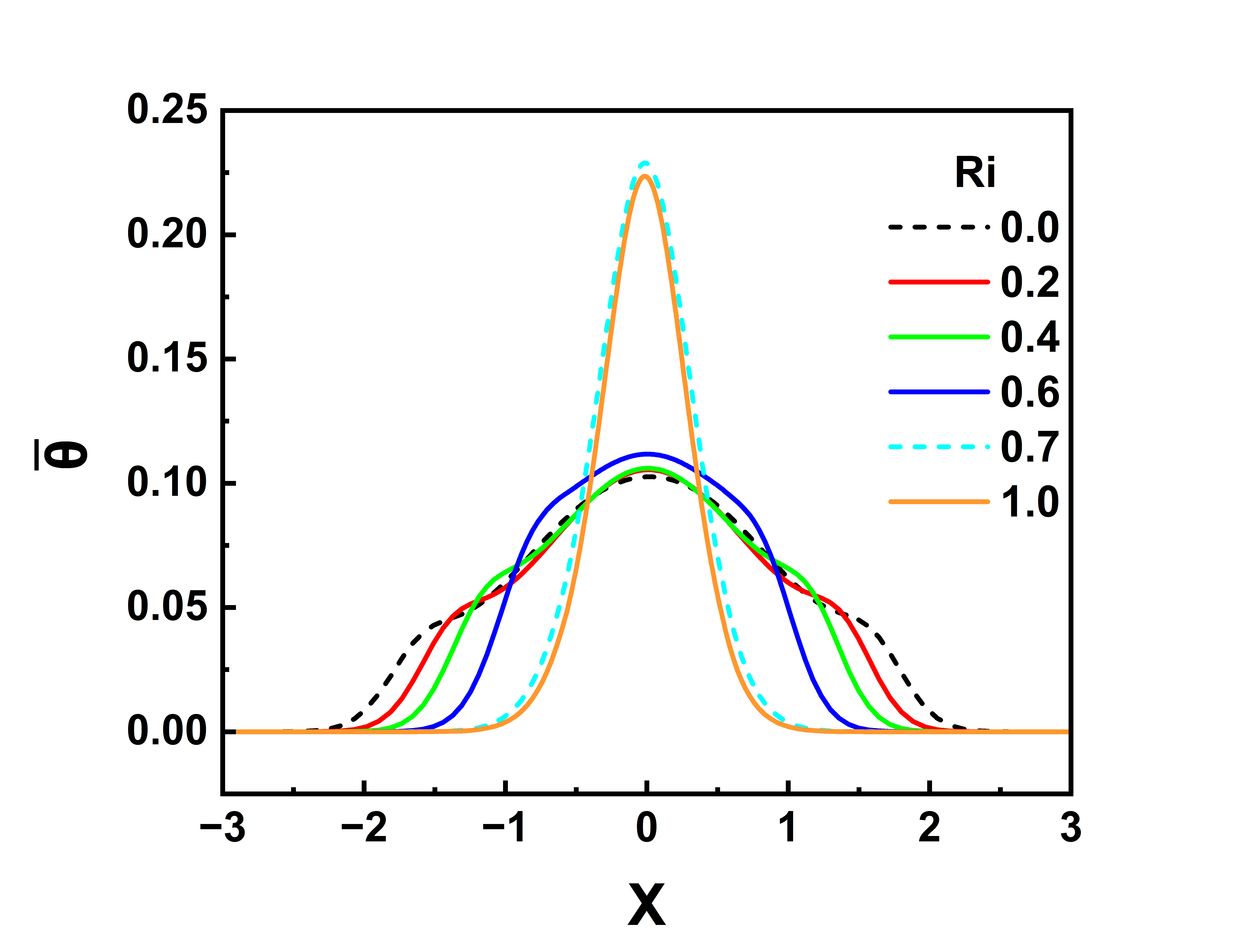
(b) Y $=5$

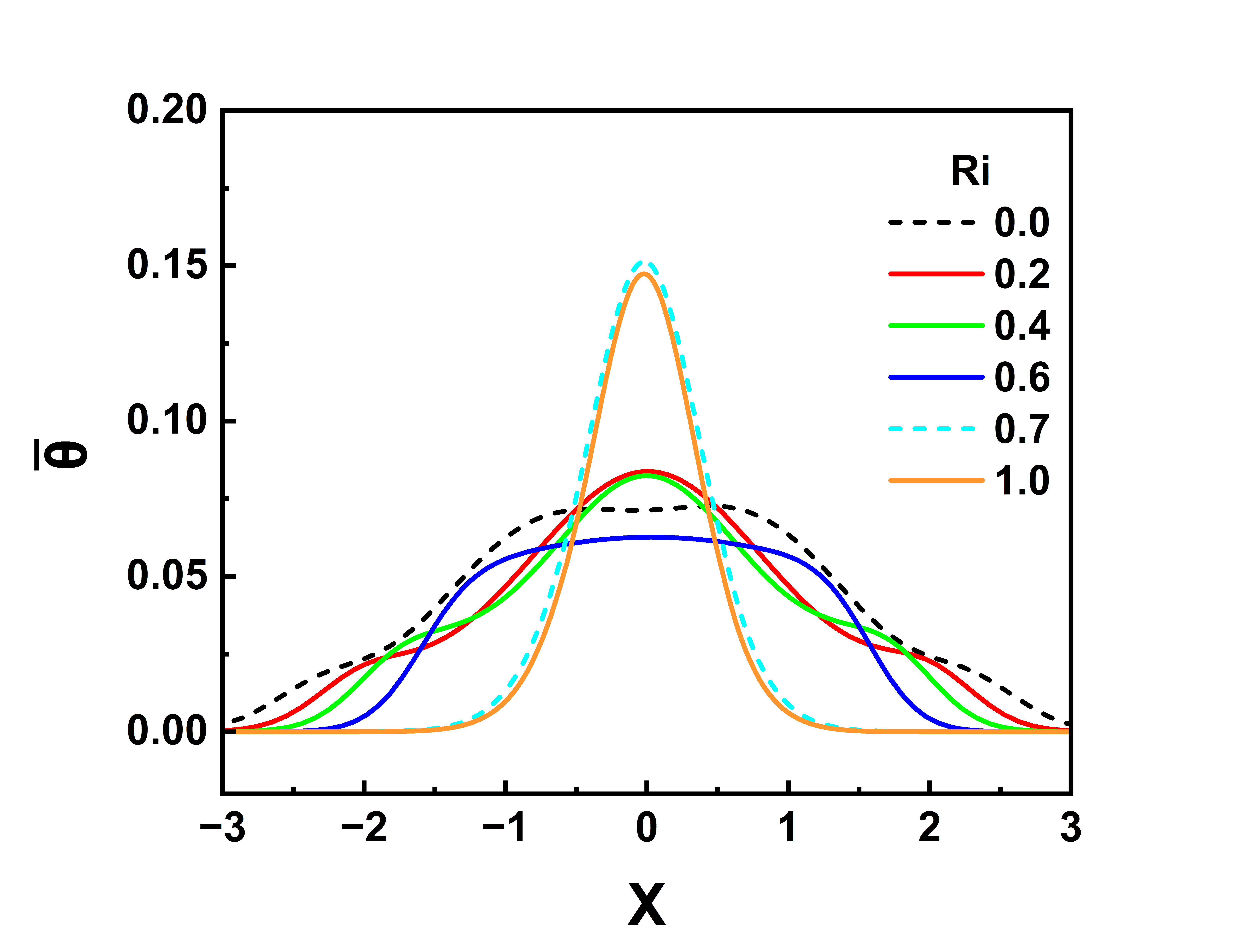
(c) Y $=10$

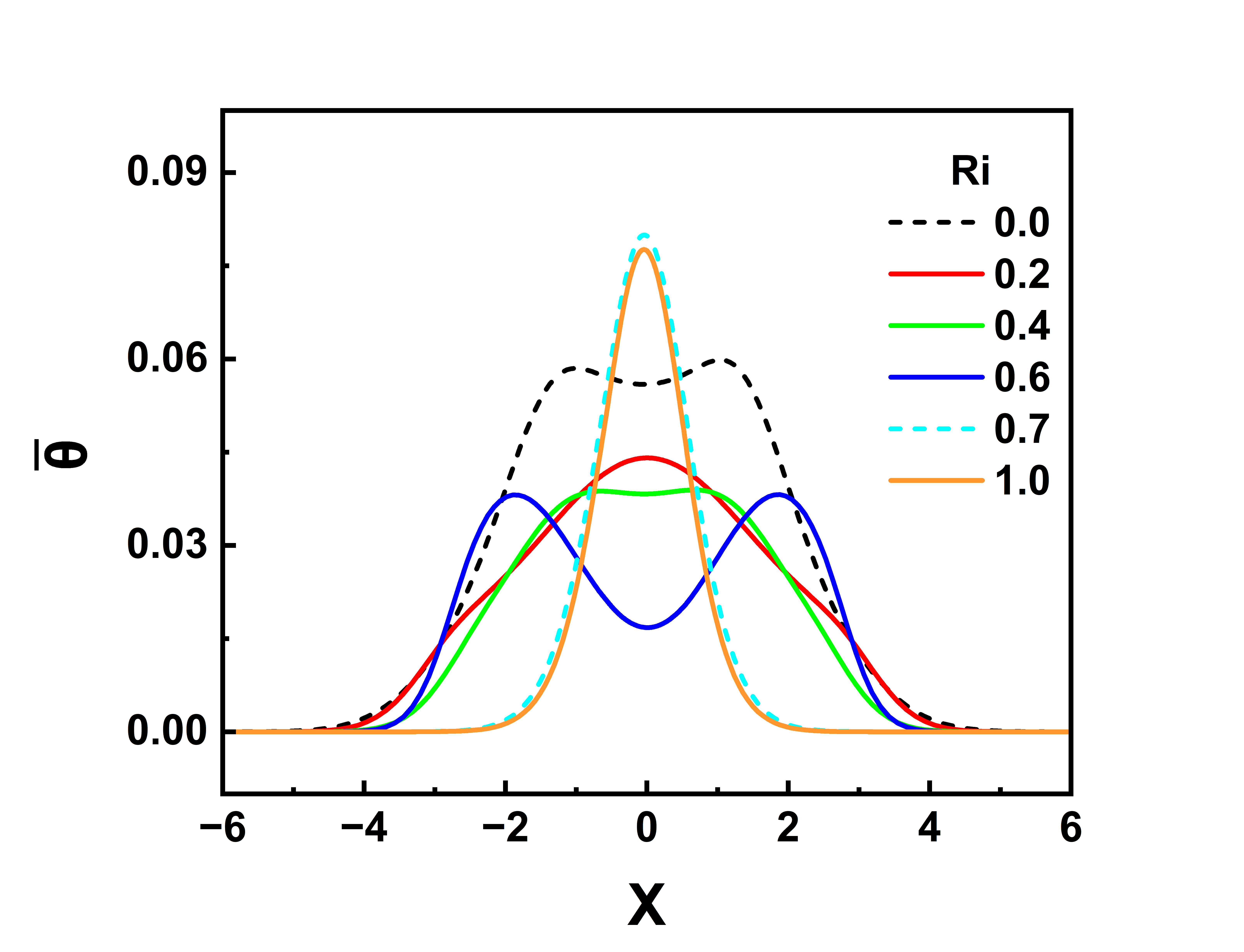
(d) Y $=30$

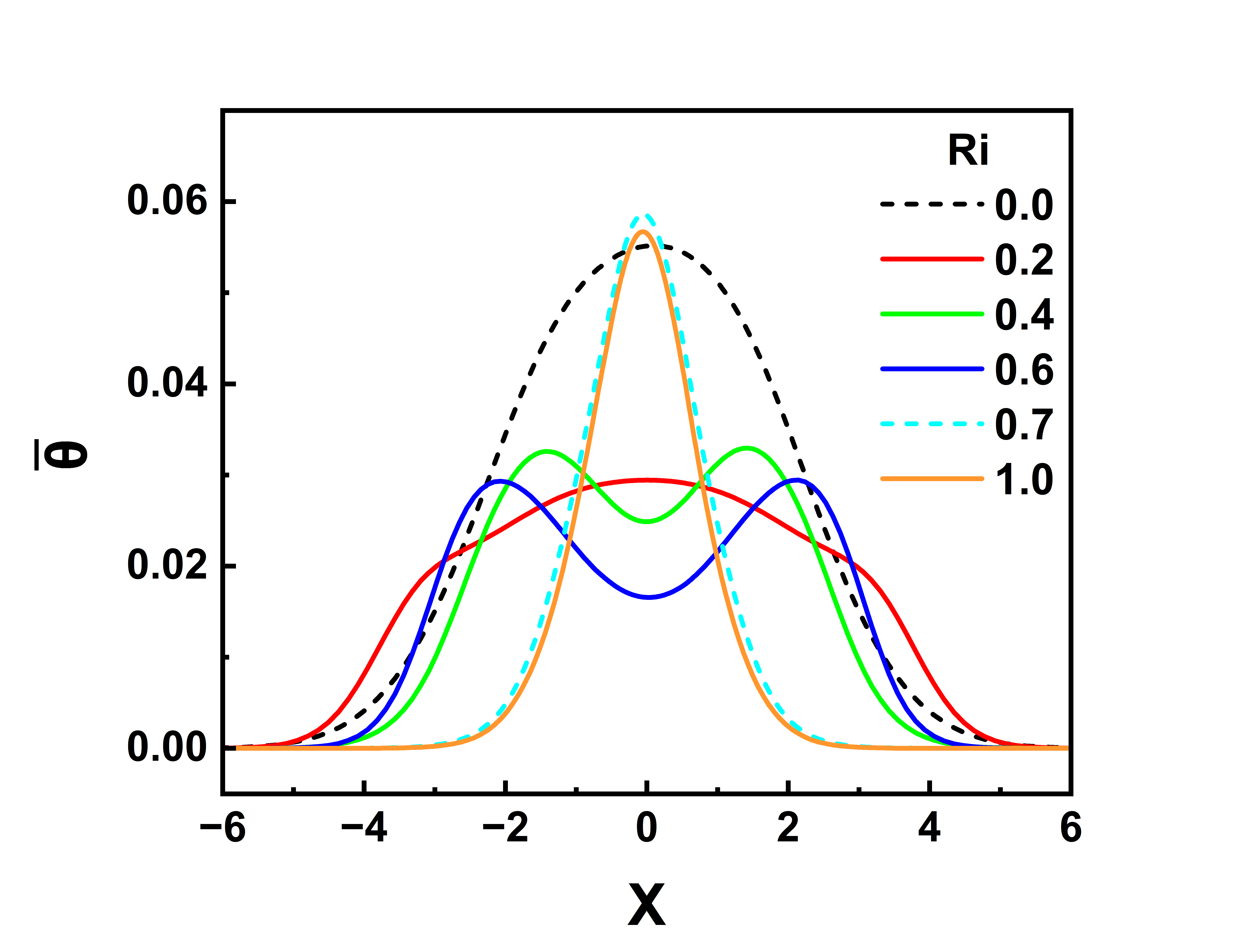
(e) Y $=50$

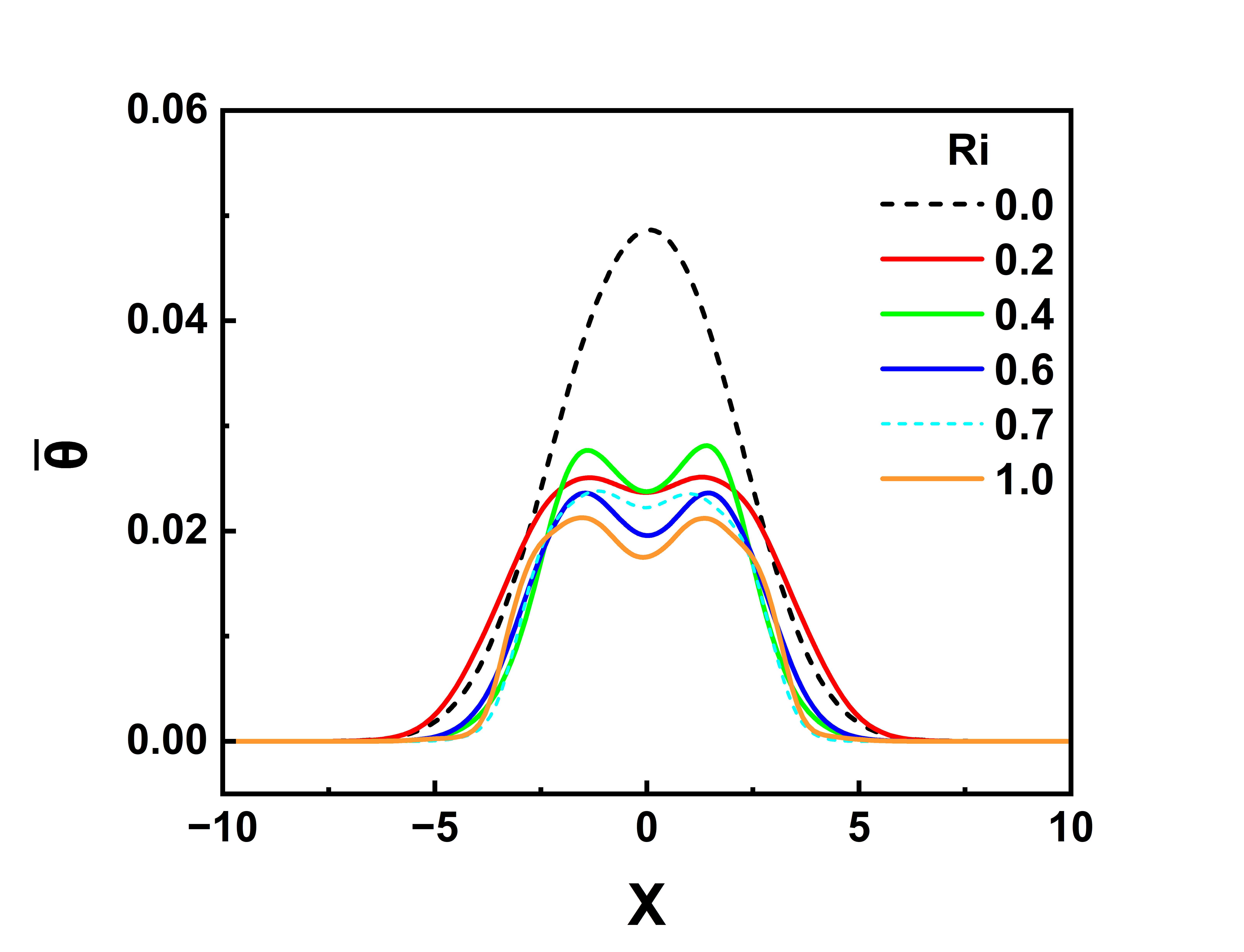
(f) Y $=80$

Figure 19: Temperature profile at (a) Y $=1$, (b) Y $=5$, (c) Y $=10$, (d) Y $=30$, (e) Y $=50$, and (f) Y $=80$.

III.4 Momentum deficit and vortex shedding suppression in the near-field

As discussed earlier, shear layer separation occurs at the downstream corners of the cylinder, leading to a deficit of velocity in the cylinder wake. Beyond a critical Re, the flow transitions to unsteadiness, and the Bénard-von Kármán vortex street is seen. However, when the cylinder is heated, density differences cause buoyancy-driven momentum addition, which causes flow acceleration in the wake, particularly around the centerline. This leads to the suppression of vortex shedding in a similar mechanism as other flow control techniques, which prevent the interaction of the two shear layers that originate at the downstream corners.

The increased momentum in the wake at higher Ri suggests that the effect of buoyancy is to add a source that effectively behaves as a jet without the addition of any new momentum, as explained below. At lower Ri, the effective jet caused by buoyancy does not possess sufficient momentum to affect the interaction between the two shear layers. As Ri is increased, a larger velocity of the effective jet causes the undulation of the oppositely signed shear layers to decrease. The interaction between the shear layers is affected by the effective jet, which behaves in a similar way as a splitter plate [43] or a blowing jet [44]. Below the critical Ri, this manifests as an increase in the recirculation length (see Figure 15) due to the increased shear layer length prior to roll-up and detachment. Additionally, the cancellation of the forced convective vorticity by the opposite natural convective vorticity inhibits the interaction between the shear layers. The hindered interaction between the shear layers leads to a loss of strength due to the inability to mutually gain further circulation, leading to a situation where detachment of the shear layers is not possible [2] and the vortices remain as a steady separation bubble with no roll-up, beyond the critical Ri of 0.68 (see Figure 4).

”Momentum deficit” or ”momentum addition” may be misunderstood as the disappearance or appearance of momentum in the domain. It is important to note that there is no disappearance or appearance of momentum in the domain. The shear layer separation at the lateral corners of the cylinder causes the flow to accelerate around the cylinder, while the flow that strikes the cylinder head-on is decelerated, leading to a large momentum deficit in the wake. Beyond the cylinder, the flow velocity near the centerline is low, while the flow velocity parallel to the centerline is high. When the cylinder is heated, the buoyancy-driven flow behaves like a jet in the downstream region, accelerating the flow around the centerline and decelerating the flow parallel to the centerline. These flow accelerations are nominally referred to as ”momentum deficit” and ”momentum addition,” respectively.

III.5 Unsteadiness of the far-field

In previous studies, the far-field unsteadiness has not been captured due to the usage of a streamwise domain length less than the onset distance of the far-field unsteadiness, resulting in an inaccurate prediction of steady flow in the entire domain. To avoid such issues and to fully capture the physics of the flow field, we have considered a downstream length ($L_{d}$) of 110d. Instantaneous and time-averaged contours in Figures 5, 3, 11 and 9 reveal that at Ri $=0.0$, the far-field is steady, while for Ri $>0.0$, the far-field is unsteady, which can be attributed to the increasing strength of the natural convective flow which makes the far-field behave like a plume. At the critical Ri and beyond, the far-field develops large-scale unsteadiness that is very similar to plume-like unsteadiness reported in the literature [24, 25, 26, 31]. This occurs in conjunction with the suppression of near-field vortex shedding. There is no range of Ri for which the flow field is entirely steady. As Ri is increased beyond the critical Ri, the point of the onset of the far-field unsteadiness appears to come closer to the cylinder, which further indicates that the plume strength increases closer to the cylinder on increasing Ri. For Ri $\leq 0.6$, there is a widening of the plume in the intermediate-field itself, and in the far-field, the plume narrows (see Figures 11 and 9). For Ri $\geq 0.7$, the plume is narrow in the near and intermediate fields, and it sharply widens in the far-field with the onset of the far-field unsteadiness. The natural convective component grows stronger with increased downstream distance, and the opposite occurs with the forced convective component. Due to this, there is a large momentum excess far downstream (Y $>$ 60) which causes strong jet-like behavior in the far-field. This can be seen in Figures 16 and 13(a). The jetting effect in the far-field is responsible for the far-field plume-like unsteadiness, which shows similar characteristics as the instabilities observed in natural convection plumes [24, 25, 26, 31]. The flow structures observed in the far-field require further detailed investigation for a complete understanding of the flow physics in the far-field.

The observed transition sequence is in contrast with that reported by Dushe [17] for the $\alpha=0^{\circ}$ case. For $\alpha=0^{\circ}$, there is a range (0.15-0.58) where the entire flow field is steady in the near-field as well as the far-field. However, for our $\alpha=45^{\circ}$ case, the flow immediately transitions from near-field unsteadiness to far-field unsteadiness, with no intermediate Ri at which there is steady flow in the entire domain. At any positive Ri, the flow is unsteady in at least one region of the domain.

IV Conclusions

In this study, we conducted a detailed examination of buoyancy-aided mixed convective flow past a square cylinder at an angle of incidence $\alpha=45^{\circ}$ for Re $=100$, $0.0\leq Ri\leq 1.0$ and Pr $=0.7$ by performing direct numerical simulations (DNS) using the finite-difference Marker and Cell (MAC) method. We evaluated different integral parameters, such as drag and lift coefficients and Nusselt number, for various Ri and observed that the time-averaged integral parameters increase with Ri, while the RMS integral parameters decrease with Ri. Using Stuart-Landau analysis, we found that the critical Ri for the suppression of vortex shedding in the near-field is 0.681, which matches that predicted by DNS excellently.

At a critical Ri of 0.68, vortex shedding suppression takes place, leading to a steady flow in the near-field, while simultaneously, the far-field develops large-scale unsteadiness similar to a plume, with no range of Ri for which the entire flow field is seen to be stable. At low Ri, the downstream flow behavior resembles that of a wake, having a deficit of momentum in the time-averaged velocity. As Ri is increased, the flow behavior gradually changes into that of a plume, which behaves like a jet, having an excess of momentum in the time-averaged velocity. However, the flow retains characteristics of a wake and shows dual wake-plume behavior in this intermediate Ri range. An inversion of vorticity takes place behind the cylinder for all positive Ri, due to the interplay between the forced and natural convective components of the flow which induce vorticities of opposite nature.

These findings provide valuable insight into the near-field and far-field dynamics of the buoyancy-aided mixed convective flows past cylinders. The suppression of vortex shedding, inversion of vorticity, and onset of the far-field plume-like unsteadiness contribute to our understanding of the characteristics of such flows.

- [1] S. Sen, S. Mittal, and G. Biswas, “Flow past a square cylinder at low Reynolds numbers,” International Journal for Numerical Methods in Fluids, vol. 67, no. 9, pp. 1160–1174, 2011.
- [2] J. H. Gerrard, “The mechanics of the formation region of vortices behind bluff bodies,” Journal of Fluid Mechanics, vol. 25, no. 2, pp. 401–413, 1966.
- [3] A. Sohankar, C. Norberg, and L. Davidson, “Low-Reynolds-number flow around a square cylinder at incidence: study of blockage, onset of vortex shedding and outlet boundary condition,” International Journal for Numerical Methods in Fluids, vol. 26, no. 1, pp. 39–56, 1998.
- [4] J. Robichaux, S. Balachandar, and S. Vanka, “Three-dimensional Floquet instability of the wake of square cylinder,” Physics of Fluids, vol. 11, no. 2-3, pp. 560–578, 1999.
- [5] A. K. Saha, K. Muralidhar, and G. Biswas, “Transition and chaos in two-dimensional flow past a square cylinder,” Journal of Engineering Mechanics, vol. 126, no. 5, pp. 523–532, 2000.
- [6] B. R. Noack and H. Eckelmann, “A global stability analysis of the steady and periodic cylinder wake,” Journal of Fluid Mechanics, vol. 270, pp. 297–330, 1994.
- [7] G. E. Karniadakis and G. S. Triantafyllou, “Three-dimensional dynamics and transition to turbulence in the wake of bluff objects,” Journal of Fluid Mechanics, vol. 238, pp. 1–30, 1992.
- [8] C. H. K. Williamson, “Vortex dynamics in the cylinder wake,” Annual Review of Fluid Mechanics, vol. 28, pp. 477–539, 1996.
- [9] A. K. Saha, Dynamical characteristics of the wake of a square cylinder at low and high Reynolds numbers. PhD thesis, Indian Institute of Technology Kanpur, 1999.
- [10] D. J. Tritton, “Experiments on the flow past a circular cylinder at low Reynolds numbers,” Journal of Fluid Mechanics, vol. 6, no. 4, p. 547–567, 1959.
- [11] A. Okajima, “Strouhal numbers of rectangular cylinders,” Journal of Fluid Mechanics, vol. 123, pp. 379–398, 1982.
- [12] A. K. Saha, K. Muralidhar, and G. Biswas, “Experimental study of flow past a square cylinder at high Reynolds numbers,” Experiments in Fluids, vol. 29, no. 6, pp. 553–563, 2000.
- [13] R. W. Davis, E. F. Moore, and L. P. Purtell, “A numerical-experimental study of confined flow around rectangular cylinders,” Physics of Fluids, vol. 27, no. 1, pp. 46–59, 1984.
- [14] S. Camarri and F. Giannetti, “On the inversion of the von Karman street in the wake of a confined square cylinder,” Journal of Fluid Mechanics, vol. 574, pp. 169–178, 2007.
- [15] H. Suzuki, Y. Inoue, T. Nishimura, K. Fukutani, and K. Suzuki, “Unsteady flow in a channel obstructed by a square rod (crisscross motion of vortex),” International Journal of Heat and Fluid Flow, vol. 14, no. 1, pp. 2–9, 1993.
- [16] K. Suzuki and H. Suzuki, “Instantaneous structure and statistical feature of unsteady flow in a channel obstructed by a square rod,” International Journal of Heat and Fluid Flow, vol. 15, no. 6, pp. 426–437, 1994.
- [17] R. Dushe, “Buoyancy-aided mixed convective flow past a heated square cylinder,” Master’s thesis, Indian Institute of Technology, Kanpur, 2023.
- [18] W. Zhang and R. Samtaney, “Numerical simulation and global linear stability analysis of low-Re flow past a heated circular cylinder,” International Journal of Heat and Mass Transfer, vol. 98, pp. 584–595, 2016.
- [19] N. Michaux-Leblond and M. Bélorgey, “Near-wake behavior of a heated circular cylinder: Viscosity-buoyancy duality,” Experimental Thermal and Fluid Science, vol. 15, no. 2, pp. 91–100, 1997.
- [20] A. Sharma and V. Eswaran, “Effect of aiding and opposing buoyancy on the heat and fluid flow across a square cylinder at Re = 100,” Numerical Heat Transfer, Part A: Applications, vol. 45, no. 6, pp. 601–624, 2004.
- [21] K.-S. Chang and J.-Y. Sa, “The effect of buoyancy on vortex shedding in the near wake of a circular cylinder,” Journal of Fluid Mechanics, vol. 220, pp. 253–266, 1990.
- [22] R. Ranjan, A. Dalal, and G. Biswas, “A numerical study of fluid flow and heat transfer around a square cylinder at incidence using unstructured grids,” Numerical Heat Transfer, Part A: Applications, vol. 54, no. 9, pp. 890–913, 2008.
- [23] A. K. Saha, “Unsteady free convection in a vertical channel with a built-in heated square cylinder,” Numerical Heat Transfer, Part A: Applications, vol. 38, no. 8, pp. 795–818, 2000.
- [24] M. Qiao, F. Xu, and S. C. Saha, “Numerical study of the transition to chaos of a buoyant plume from a two-dimensional open cavity heated from below,” Applied Mathematical Modelling, vol. 61, pp. 577–592, 2018.
- [25] M. Qiao, Z. F. Tian, B. Nie, and F. Xu, “The route to chaos for plumes from a top-open cylinder heated from underneath,” Physics of Fluids, vol. 30, no. 12, pp. 124–102, 2018.
- [26] Y. Jiang, Y. Zhao, J. Carmeliet, B. Nie, and F. Xu, “Critical transitions on a route to chaos of natural convection on a heated horizontal circular surface,” Journal of Fluid Mechanics, vol. 988, p. A38, 2024.
- [27] D.-H. Yoon, K.-S. Yang, and C.-B. Choi, “Flow past a square cylinder with an angle of incidence,” Physics of Fluids, vol. 22, no. 4, p. 043603, 2010.
- [28] M. Arif and N. Hasan, “Effect of thermal buoyancy on vortex-shedding and aerodynamic characteristics for fluid flow past an inclined square cylinder,” International Journal of Heat and Technology, vol. 38, no. 2, pp. 463–471, 2020.
- [29] J. P. Dulhani, S. Sarkar, and A. Dalal, “Effect of angle of incidence on mixed convective wake dynamics and heat transfer past a square cylinder in cross flow at Re=100,” International Journal of Heat and Mass Transfer, vol. 74, pp. 319–332, 2014.
- [30] A. A. Kakade, S. K. Singh, P. K. Panigrahi, and K. Muralidhar, “Schlieren investigation of the square cylinder wake: Joint influence of buoyancy and orientation,” Physics of Fluids, vol. 22, no. 5, p. 054107, 2010.
- [31] S. Kimura and A. Bejan, “Mechanism for transition to turbulence in buoyant plume flow,” International Journal of Heat and Mass Transfer, vol. 26, no. 10, pp. 1515–1532, 1983.
- [32] I. Orlanski, “A simple boundary condition for unbounded hyperbolic flows,” Journal of Computational Physics, vol. 21, no. 3, pp. 251–269, 1976.
- [33] F. H. Harlow and J. E. Welch, “Numerical calculation of time-dependent viscous incompressible flow of fluid with free surface,” Physics of Fluids, vol. 8, no. 12, pp. 2182–2189, 1965.
- [34] J. T. Stuart, “On the non-linear mechanics of hydrodynamic stability,” Journal of Fluid Mechanics, vol. 4, no. 1, p. 1–21, 1958.
- [35] J. T. Stuart, “On the non-linear mechanics of wave disturbances in stable and unstable parallel flows part 1. The basic behaviour in plane Poiseuille flow,” Journal of Fluid Mechanics, vol. 9, no. 3, p. 353–370, 1960.
- [36] J. Watson, “On the non-linear mechanics of wave disturbances in stable and unstable parallel flows part 2. The development of a solution for plane Poiseuille flow and for plane Couette flow,” Journal of Fluid Mechanics, vol. 9, no. 3, p. 371–389, 1960.
- [37] E. Palm, “On the tendency towards hexagonal cells in steady convection,” Journal of Fluid Mechanics, vol. 8, no. 2, p. 183–192, 1960.
- [38] M. Provansal, C. Mathis, and L. Boyer, “Bénard-von Kármán instability: transient and forced regimes,” Journal of Fluid Mechanics, vol. 182, p. 1–22, 1987.
- [39] J. Dušek, P. L. Gal, and P. Fraunié, “A numerical and theoretical study of the first Hopf bifurcation in a cylinder wake,” Journal of Fluid Mechanics, vol. 264, p. 59–80, 1994.
- [40] R. Godoy-Diana, J.-L. Aider, and J. E. Wesfreid, “Transitions in the wake of a flapping foil,” Physical Review E, vol. 77, p. 016308, 2008.
- [41] T. Schnipper, A. Andersen, and T. Bohr, “Vortex wakes of a flapping foil,” Journal of Fluid Mechanics, vol. 633, p. 411–423, 2009.
- [42] K. D. Jones, C. M. Dohring, and M. F. Platzer, “Experimental and computational investigation of the Knoller-Betz effect,” AIAA Journal, vol. 36, no. 7, pp. 1240–1246, 1998.
- [43] A. Saha and R. Jaiswal, “Control of vortex shedding past a square cylinder using splitter plate at low Reynolds number,” in Proceedings of the 38th National Conference on Fluid Mechanics and Fluid Power, (Maulana Azad National Institute of Technology, Bhopal, India), 2011.
- [44] A. Saha and A. Shrivastava, “Suppression of vortex shedding around a square cylinder using blowing,” Sadhana, vol. 40, 2015.