Neutrino Electromagnetic Properties

Abstract

Neutrinos are neutral in the Standard Model, but they have tiny charge radii generated by radiative corrections. In theories Beyond the Standard Model, neutrinos can also have magnetic and electric moments and small electric charges (millicharges). We review the general theory of neutrino electromagnetic form factors, which reduce, for ultrarelativistic neutrinos and small momentum transfers, to the neutrino charges, effective charge radii, and effective magnetic moments. We discuss the phenomenology of these electromagnetic neutrino properties and we review the existing experimental bounds. We briefly review also the electromagnetic processes of astrophysical neutrinos and the neutrino magnetic moment portal in the presence of sterile neutrinos.

1 Introduction

Neutrinos are the most elusive among all the known elementary particles because their interactions with matter particles (quarks and electrons) are feeble. For this reason, some of their fundamental properties are not known: most important are the absolute values of the neutrino masses and if neutrinos are Dirac fermions, endowed with corresponding antiparticles as quarks and charged leptons, or Majorana fermions, which coincide with their antiparticles.

Most of the experimentally known properties of neutrinos are in agreement with the Standard Model (SM) of electroweak interactions. The most important exception is the fact that neutrinos are massive, contrary to the SM prediction, as was discovered in oscillation experiments (see, e.g., Refs.1, 2, 3). Therefore, the SM must be extended to accommodate neutrino masses. There are also other reasons to extend the SM, as the necessity to explain the plausible existence of Dark Matter and Dark Energy and the matter-antimatter asymmetry in the Universe. There are many models which perform these tasks and implement the so-called new physics Beyond the Standard Model (BSM) [4].

In the SM neutrinos are electrically neutral and do not interact directly (i.e. at the tree level) with electromagnetic fields. Therefore, the only electromagnetic properties of neutrinos in the SM are the tiny charge radii generated by radiative corrections. In BSM models neutrinos can have also magnetic and electric moments, which are often proportional to the neutrino masses, and tiny electric charges.

The neutrino magnetic moment $\mu_{\nu}$ was introduced by Wolfgang Pauli in his famous letter [5] addressed to ”Dear Radioactive Ladies and Gentlemen” of the Tübingen meeting of the German Physical Society on December 1930. The impact of neutrinos with nonzero magnetic moment propagating in matter was studied for the first time in 1932 by Carlson and Oppenheimer [6]. The cross section of magnetic moment interaction of a neutrino with an electron was calculated by Bethe in 1935 [7]. Before the first observation of neutrinos by Cowan and Reines in 1956 [8] through the inverse beta decay (IBD) process $\nu_{e}+p\to n+e^{+}$, whose cross section was estimated to be extremely small by Bethe and Peierls [9], the magnetic moment interaction was considered as an alternative process for detecting neutrinos if the neutrino magnetic moment is large enough. The first attempt to detect neutrinos through its magnetic moment interaction was done in 1935 by Nahmias [10] with two Geiger-Müller counters placed near a radioactive source. The neutrinos were not detected and Nahmias established the upper bound $\mu_{\nu}<2\times 10^{-4}\,\mu_{\text{B}}$. Before their first observation of neutrinos in 1956 [8], in 1954 Cowan and Reines attempted to measure the neutrino magnetic moment with a liquid scintillation detector exposed to the electron antineutrino flux of the Savannah River reactor. They obtained the upper limit $\mu_{\nu}<10^{-7}\mu_{\text{B}}$ [11]. Later, in 1957, they obtained $\mu_{\nu}<10^{-9}\mu_{\text{B}}$ [12] with a larger and better-shielded detector. Since then, the electromagnetic properties and interactions of neutrinos have been studied in many theoretical and experimental works (see, e.g., Refs.13, 14, 15, 16, 17, 18, 19, 20 and references therein).

In this review, first we briefly review in Section 2 the phenomenology of neutrino mixing and oscillations, which is useful for the following discussion of neutrino electromagnetic properties. In Section 3 we review the general theory of the electromagnetic properties of massive Dirac and Majorana neutrinos. In Sections 4, 5, and 6 we review the theory of neutrino magnetic moments, charge radii, and electric charges (sometimes called “millicharges”) and we present the current bounds obtained directly from experiments and from phenomenological analyses of experimental data. In Section 7 we review the phenomenology of the most important electromagnetic processes of astrophysical neutrinos. In Section 8 we review the so-called “neutrino magnetic moment portal” or “neutrino dipole moment portal”, which is currently considered an interesting theoretical possibility. Finally, in Section 9 we conclude and briefly indicate the future experiments which can improve the search of neutrino electromagnetic interactions.

2 Neutrino mixing and oscillations

We know that there are three active neutrino flavors: $\nu_{e}$, $\nu_{\mu}$, and $\nu_{\tau}$, which produce the corresponding charged leptons $e$, $\mu$, and $\tau$ in charged-current weak interactions. In the minimal framework of three-neutrino mixing (see, e.g., Refs.1, 2, 3), the three flavor neutrinos are superpositions of three massive neutrinos $\nu_{1}$, $\nu_{2}$, and $\nu_{3}$, given by

$$|\nu_{\ell}\rangle=\sum_{k=1}^{3}U_{\ell k}^{*}\,|\nu_{k}\rangle,\quad\text{for}\quad\ell=e,\mu,\tau,$$ (1)

where $U$ is the $3\times 3$ unitary mixing matrix. Neutrino oscillations are flavor transitions which depend on the elements of the mixing matrix $U$ and on the squared-mass differences $\Delta{m}^{2}_{kj}\equiv m_{k}^{2}-m_{j}^{2}$. The massive neutrinos can be either of Dirac or Majorana type. In the Dirac case, there are distinct neutrino and antineutrino states, whereas in the Majorana case neutrino and antineutrino coincide. The helicity of active Dirac neutrinos is left-handed and that of active Dirac antineutrinos is right-handed. Active Majorana neutrinos can be either left-handed or right-handed. Hence, it is convenient to call “neutrino” both a left-handed Dirac neutrino or a left-handed Majorana neutrino and to call “antineutrino” both a right-handed Dirac antineutrino or a right-handed Majorana neutrino. Antineutrinos obey a mixing relation similar to 1, with $U^{*}\to U$. The three neutrino masses are constrained below about 1 eV by kinematical measurements [1].

The $3\times 3$ unitary mixing matrix can be parameterized in terms of three mixing angles, one Dirac CP-violating phase, and two Majorana CP-violating phases in the case of Majorana neutrinos. Neglecting the Majorana phases, which are completely unknown and do not have any effect on neutrino oscillations, except in the case of neutrino spin oscillations in the presence of magnetic fields and matter (see Section 7.5), the standard parameterization of the mixing matrix is

$$U=\begin{pmatrix}c_{12}c_{13}&s_{12}c_{13}&s_{13}e^{-i\delta_{13}}\\ -s_{12}c_{23}-c_{12}s_{23}s_{13}e^{i\delta_{13}}&c_{12}c_{23}-s_{12}s_{23}s_{13}e^{i\delta_{13}}&s_{23}c_{13}\\ s_{12}s_{23}-c_{12}c_{23}s_{13}e^{i\delta_{13}}&-c_{12}s_{23}-s_{12}c_{23}s_{13}e^{i\delta_{13}}&c_{23}c_{13}\end{pmatrix},$$ (2)

where $c_{ab}\equiv\cos\vartheta_{ab}$ and $s_{ab}\equiv\sin\vartheta_{ab}$. The values of the three mixing angles $\vartheta_{12}$, $\vartheta_{23}$, and $\vartheta_{13}$ are constrained between $0$ and $\pi/2$, whereas the value of the Dirac CP-violating phase $\delta_{13}$ can be between $0$ and $2\pi$. This parameterization is convenient because it has the simplest form of the first line concerning electron neutrinos, which are produced and/or detected in many experiments. It is also convenient because the CP-violating phase $\delta_{13}$ is associated with the smallest mixing angle $\vartheta_{13}$ and it is clear that the amount of CP violation is proportional to $\sin\vartheta_{13}$.

Neutrino oscillations have been discovered in 1998 in the Super-Kamiokande atmospheric neutrino experiment [21] and later confirmed in several long-baseline accelerator and reactor experiments and in solar neutrino experiments (see, e.g., Refs.1, 2, 3). The analysis of the data of these experiments established that $\Delta{m}^{2}_{21}\ll|\Delta{m}^{2}_{31}|$, where $\Delta{m}^{2}_{21}>0$ by convention ($m_{2}>m_{1}$), but the sign of $\Delta{m}^{2}_{31}$ is not known. Hence, there are two possible orderings of the neutrino masses: the normal ordering (NO) with $m_{1}<m_{2}<m_{3}$ and $\Delta{m}^{2}_{31},\,\Delta{m}^{2}_{32}>0$; the inverted ordering (IO) with $m_{3}<m_{1}<m_{2}$ and $\Delta{m}^{2}_{31},\,\Delta{m}^{2}_{32}<0$. The best-fit values of the oscillation parameters obtained from a global fit of neutrino oscillation data [22] (see also the similar results obtained in Refs.23, 24) are

$$\begin{array}[]{ll}\displaystyle\Delta{m}^{2}_{21}=7.50^{+0.22}_{-0.20}\times 10^{-5}\,\text{eV}^{2},&\displaystyle\sin^{2}\vartheta_{12}=0.318\pm 0.016,\\ \displaystyle\Delta{m}^{2}_{31}|_{\text{NO}}=2.55^{+0.02}_{-0.03}\times 10^{-3}\,\text{eV}^{2},&\displaystyle\Delta{m}^{2}_{31}|_{\text{IO}}=-2.45^{+0.02}_{-0.03}\times 10^{-3}\,\text{eV}^{2},\\ \displaystyle\left.\sin^{2}\vartheta_{23}\right|_{\text{NO}}=0.574\pm 0.014,&\displaystyle\left.\sin^{2}\vartheta_{23}\right|_{\text{IO}}=0.578^{+0.010}_{-0.017},\\ \displaystyle\left.\sin^{2}\vartheta_{13}\right|_{\text{NO}}=0.02200^{+0.00069}_{-0.00062},&\displaystyle\left.\sin^{2}\vartheta_{13}\right|_{\text{IO}}=0.02225^{+0.00064}_{-0.00070}\\ \displaystyle\left.\delta_{13}\right|_{\text{NO}}=1.08^{+0.13}_{-0.12}\pi,&\displaystyle\left.\delta_{13}\right|_{\text{IO}}=1.58^{+0.15}_{-0.16}\pi,\end{array}$$ (3)

The best-fit values of $|\Delta{m}^{2}_{31}|$, $\sin^{2}\vartheta_{23}$, $\sin^{2}\vartheta_{13}$, and $\delta_{13}$ are slightly different in the NO and IO. There is a $2.5\sigma$ preference for NO, which however is not considered as the definitive establishment of NO. The issue is under investigation in new experiments (JUNO [25], DUNE [26], Hyper-Kamiokande [27], ESSnuSB [28]). Although the mixing angle $\vartheta_{23}$ seems to be relatively well-determined from the $1\sigma$ uncertainties in Eq.3, it is the less known mixing angle, with $3\sigma$ ranges $\left.\sin^{2}\vartheta_{23}\right|_{\text{NO}}\in(0.434,0.610)$ and $\left.\sin^{2}\vartheta_{23}\right|_{\text{IO}}\in(0.433,0.608)$. Therefore, it is not known if $\vartheta_{23}$ is smaller, larger or equal to the maximal mixing value of $\pi/4$ (i.e. $\sin^{2}\vartheta_{23}=0.5$).

3 Electromagnetic properties of massive Dirac and Majorana neutrinos

Neutrinos are generally believed to be neutral particles which do not have electromagnetic interactions. This belief stems from the fact that in the SM neutrinos are exactly neutral and there are no electromagnetic interactions at the tree-level. However, even in the SM neutrinos are predicted to have small electromagnetic interactions due to the so-called “charge radius” [29, 30, 31, 32] which is generated by radiative corrections. Moreover, in BSM theories, neutrinos can have additional electromagnetic interactions.

The electromagnetic properties of neutrinos are derived from a general description of neutrino electromagnetic interactions in the one-photon approximation through the effective interaction Hamiltonian

$$\mathcal{H}_{\text{em}}^{(\nu)}(x)=j^{\mu}_{(\nu)}(x)A_{\mu}(x),$$ (4)

where $A_{\mu}(x)$ is the electromagnetic field and

$$j^{\mu}_{(\nu)}(x)=\sum_{k,j}\overline{\nu_{k}}(x)\widehat{\Lambda}^{\mu}_{kj}\nu_{j}(x)$$ (5)

is the effective electromagnetic current four-vector. $\widehat{\Lambda}^{\mu}_{kj}$ is the effective electromagnetic operator in spinor space. The sum in Eq.5 is over the indices $k,j=1,2,3,\ldots$ of the massive neutrinos, which are three in the case of standard three-neutrino mixing, but can be more if additional sterile neutrinos exist [33, 34, 35, 36, 37, 38]. The effective electromagnetic current $j^{\mu}_{(\nu)}(x)$ acts between neutrino massive states in the calculation of electromagnetic interactions represented by the Feynman diagram in Fig.1:

$$\langle\nu_{f}(p_{f})|j^{\mu}_{(\nu)}(x)|\nu_{i}(p_{i})\rangle=e^{i(p_{f}-p_{i})x}\,\overline{u_{f}}(p_{f})\Lambda^{\mu}_{fi}(q)u_{i}(p_{i}),$$ (6)

where the vertex function $\Lambda^{\mu}_{fi}(q)$ is a $4\times 4$ matrix in spinor space which depends on the four-momentum transfer $q=p_{i}-p_{f}$ (the four-momentum of the photon in Fig.1). The vertex function can be decomposed in a sum of linearly independent products of Dirac $\gamma$ matrices. Then, from the hermiticity of the interaction Hamiltonian 4 and gauge invariance, it can be reduced to

$$\Lambda^{\mu}_{fi}(q)=\left(\gamma^{\mu}-q^{\mu}\not{q}/q^{2}\right)\left[F^{Q}_{fi}(q^{2})+F^{A}_{fi}(q^{2})q^{2}\gamma_{5}\right]-i\sigma^{\mu\nu}q_{\nu}\left[F^{M}_{fi}(q^{2})+iF^{E}_{fi}(q^{2})\gamma_{5}\right],$$ (7)

with the four charge ($F^{Q}_{fi}(q^{2})$), anapole ($F^{A}_{fi}(q^{2})$), magnetic ($F^{M}_{fi}(q^{2})$), and electric ($F^{E}_{fi}(q^{2})$) form factors, having the following main characteristics:

1. The matrices of the form factors $F^{X}$, for $X=Q,A,M,E$, are Hermitian:

   $$F^{X}=F^{X\dagger}\quad\Longleftrightarrow\quad F^{X}_{fi}=(F^{X}_{if})^{*}.$$ (8)

   Therefore, the diagonal form factors $F^{X}_{ii}$ are real.

2. For antineutrinos

   $$\overline{F}^{X}=-(F^{X})^{T}=-(F^{X})^{*}\hbox{} \hbox{}\quad\Longleftrightarrow\quad\overline{F}^{X}_{fi}=-F^{X}_{if}=-(F^{X}_{fi})^{*}\quad\text{for}\quad X=Q,M,E,$$ (9)

   $$\overline{F}^{A}=(\overline{F}^{A})^{T}=(\overline{F}^{A})^{*}\hbox{} \hbox{}\quad\Longleftrightarrow\quad\overline{F}^{A}_{fi}=F^{A}_{if}=(F^{A}_{fi})^{*}.$$ (10)

   Therefore, the real diagonal charge, magnetic and electric form factors of antineutrinos have the same size and opposite signs of those of neutrinos ($\overline{F}^{Q}_{ii}=-F^{Q}_{ii}$, $\overline{F}^{M}_{ii}=-F^{M}_{ii}$, and $\overline{F}^{E}_{ii}=-F^{E}_{ii}$), as expected. The real diagonal anapole form factors are the same for neutrinos and antineutrinos.

3. For Majorana neutrinos the neutrino-antineutrino equality implies that the matrices of the charge, magnetic and electric form factors are antisymmetric and the matrix of the anapole form factor is symmetric:

   $$F^{X}=-(F^{X})^{T}=-(F^{X})^{*}\hbox{} \hbox{}\quad\Longleftrightarrow\quad F^{X}_{fi}=-F^{X}_{if}=-(F^{X}_{fi})^{*}\quad\text{for}\quad X=Q,M,E,$$ (11)

   $$F^{A}=(F^{A})^{T}=(F^{A})^{*}\hbox{} \hbox{}\quad\Longleftrightarrow\quad F^{A}_{fi}=F^{A}_{if}=(F^{A}_{fi})^{*}.$$ (12)

   Therefore, Majorana neutrinos do not have diagonal charge, magnetic, and electric form factors ($F^{X}_{ii}=0$ for $X=Q,M,E$), but can have off-diagonal imaginary charge, magnetic, and electric form factors $F^{Q}_{fi}$, $F^{M}_{fi}$, and $F^{E}_{fi}$ for $f\neq i$. On the other hand, Majorana neutrinos can have real diagonal and off-diagonal anapole form factors.

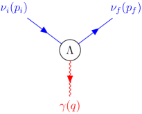
Figure 1: Effective coupling of massive neutrinos with a photon. The initial ($\nu_{i}$) and final ($\nu_{f}$) massive neutrinos can be different.

For the coupling with a real photon ($q^{2}=0$) the four form factors reduce, respectively, to the electric charge $Q_{fi}$, anapole $A_{fi}$, magnetic moment $\mu_{fi}$, and electric moment $\varepsilon_{fi}$ matrices of massive neutrinos. Although this limit of a constant value is strictly true only for $q^{2}=0$, it has been so far adopted also for electromagnetic neutrino interactions mediated by virtual photons ($q^{2}\neq 0$), because there is no theoretical prediction for the $q^{2}$ dependence of the form factors. Only the first-order $q^{2}$ dependence of the charge form factors $F^{Q}_{fi}(q^{2})$ corresponding to the massive neutrino charge radii $\langle r_{fi}^{2}\rangle$ is considered:

$$F^{Q}_{fi}(q^{2})\simeq F^{Q}_{fi}(0)+q^{2}\left.\dfrac{dF^{Q}_{fi}(q^{2})}{dq^{2}}\right|_{q^{2}=0}=Q_{fi}+\dfrac{q^{2}}{6}\,\langle r_{fi}^{2}\rangle.$$ (13)

The reason is that the SM predicts the existence of small neutrino charge radii (see Section 5) which must be taken into account. Moreover, if neutrinos are neutral ($Q_{fi}=0$), as predicted by the SM and many BSM theories, the leading contributions of the charge form factors to neutrino electromagnetic interactions at low $q^{2}$ are given by the charge radii.

Since in Eq.6 the vertex function is inserted among the spinors of ultrarelativistic left-handed neutrinos, the effect of $\gamma_{5}$ is a simple change of sign of the anapole and electric moment terms. Therefore, at low $q^{2}$ the vertex function can be reduced to the effective form

$$\Lambda^{\mu}_{fi}(q)=\left(\gamma^{\mu}-q^{\mu}\not{q}/q^{2}\right)\left[Q_{fi}+q^{2}\langle r_{fi}^{2}\rangle/6-q^{2}A_{fi}\right]-i\sigma^{\mu\nu}q_{\nu}\left[\mu_{fi}-i\varepsilon_{fi}\right].$$ (14)

The term $q_{\mu}\not{q}/q^{2}$ can be omitted, because it disappears for the coupling with a real photon, as in radiative neutrino decay $\nu_{i}\to\nu_{f}+\gamma$, where it is multiplied to the transverse photon polarization vector, and in scattering processes where it is multiplied to a conserved current. Hence, we consider the effective vertex function

$$\Lambda^{\mu}_{fi}(q)=\gamma^{\mu}\left[Q_{fi}+q^{2}\langle r_{fi}^{2}\rangle^{\text{eff}}/6\right]-i\sigma^{\mu\nu}q_{\nu}\mu_{fi}^{\text{eff}},$$ (15)

where now $\langle r_{fi}^{2}\rangle^{\text{eff}}$ are effective charge radii which include possible anapole contributions and $\mu_{fi}^{\text{eff}}$ are effective magnetic moments which include possible electric moment contributions. Note that, from item (c) above Majorana neutrinos can have diagonal effective charge radii given by the anapole contributions. However, for simplicity in the following we neglect the anapole and electric moment contributions and we drop the “eff” superscript.

An important property of the effective vertex function is that the charge and charge radius terms conserve the helicity of ultrarelativistic neutrinos, as the SM weak interaction, whereas the magnetic moment term flips the helicity. Therefore, the contributions of the charge and charge radius to the cross section of any process is coherent with the SM contribution and must be added to the amplitude of the process. On the other hand the contribution of the magnetic moment is incoherent with the SM contribution and must be added to the cross section of the process.

So far we have considered the neutrino electromagnetic form factors in the mass basis, where they are well-defined because massive neutrinos have definite four-momenta which are required to write Eq.6. Since the flavor neutrinos defined in Eq.1 are superpositions of different massive neutrinos with different masses, they do not have definite four-momenta. However, if we neglect the small differences of the neutrino masses in the electromagnetic interactions, we can define the electromagnetic form factors in the flavor basis through the matrix element

$$\langle\nu_{\ell^{\prime}}(p_{f})|j^{\mu}_{(\nu)}(x)|\nu_{\ell}(p_{i})\rangle=\sum_{j,k}U_{\ell^{\prime}j}\langle\nu_{j}(p_{f})|j^{\mu}_{(\nu)}(x)|\nu_{k}(p_{i})\rangle U_{\ell k}^{*}.$$ (16)

Then, from Eqs.6 and 7 we obtain, for $X=Q,A,M,E$,

$$\Lambda^{\mu}_{\ell^{\prime}\ell}=\sum_{j,k}U_{\ell^{\prime}j}\Lambda^{\mu}_{jk}U_{\ell k}^{*}\quad\Rightarrow\quad F^{X}_{\ell^{\prime}\ell}=\sum_{j,k}U_{\ell^{\prime}j}F^{X}_{jk}U_{\ell k}^{*}.$$ (17)

Since the transformation from the mass basis to the flavor basis is unitary, the hermiticity of the electromagnetic form factors in the mass basis is preserved in the flavor basis. The form factors of flavor antineutrinos are given by the unitary transformation 17 with $U\to U^{*}$. Therefore, we have

$$\overline{F}^{X}_{\ell\ell^{\prime}}=-F^{X}_{\ell^{\prime}\ell}=-(F^{X}_{\ell\ell^{\prime}})^{*}\quad\text{for}\quad X=Q,M,E,\quad\text{and}\quad\overline{F}^{A}_{\ell\ell^{\prime}}=F^{A}_{\ell^{\prime}\ell}=(F^{A}_{\ell\ell^{\prime}})^{*},$$ (18)

as in the mass basis (Eqs.9 and 10). In particular, the real diagonal charge, magnetic and electric form factors of flavor antineutrinos have the same size and opposite signs of those of flavor neutrinos, as expected. For Majorana neutrinos the antisymmetry in Eq.11 of the charge, magnetic and electric form factors in the mass basis is not preserved in the flavor basis by the unitary transformation 17 if the mixing matrix $U$ is not real (i.e. if there are Dirac or Majorana CP-violating phases). Therefore, in general also Majorana neutrinos can have real diagonal charge, magnetic and electric form factors in the flavor basis. This is not in contradiction with Eq.18 because the Majorana neutrino-antineutrino equality is not valid in the flavor basis if the mixing matrix $U$ is not real.

4 Neutrino magnetic moment

The magnetic moments are the most studied neutrino electromagnetic properties, because they can be generated in many models with massive neutrinos. The magnetic moments $\mu_{kj}^{\text{D}}$ of massive Dirac neutrinos are generated by the effective dimension-five interaction Lagrangian

$$\mathcal{L}_{\text{mag}}^{\text{D}}=-\dfrac{1}{2}\sum_{k,j}\overline{\nu_{k}}\,\sigma^{\alpha\beta}\mu_{kj}^{\text{D}}\nu_{j}\,F_{\alpha\beta}=-\dfrac{1}{2}\sum_{k,j}\overline{\nu_{kL}}\,\sigma^{\alpha\beta}\mu_{kj}^{\text{D}}\nu_{jR}\,F_{\alpha\beta}+\text{h.c.},$$ (19)

where $\nu_{kL}$ and $\nu_{kR}$ are the left-handed and right-handed components of the Dirac neutrino field $\nu_{k}=\nu_{kL}+\nu_{kR}$, and $F_{\alpha\beta}=\partial_{\alpha}A_{\beta}-\partial_{\beta}A_{\alpha}$ is the electromagnetic tensor. In the simplest extension of the SM with three massive Dirac neutrinos, the magnetic moments are given by [39, 40, 41, 42, 43, 16]

$$\mu_{kj}^{\text{D}}\simeq\frac{3eG_{\text{F}}}{16\sqrt{2}\pi^{2}}\left(m_{k}+m_{j}\right)\left(\delta_{kj}-\frac{1}{2}\sum_{\ell=e,\mu,\tau}U^{*}_{\ell k}U_{\ell j}\frac{m_{\ell}^{2}}{m_{W}^{2}}\right),$$ (20)

where $e$ is the elementary charge, $G_{\text{F}}$ is the Fermi constant, $m_{k}$ are the neutrino masses for $k=1,2,3$, $m_{\ell}$ are the charged lepton masses for $\ell=e,\mu,\tau$, and $m_{W}$ is the $W$-boson mass. Note that the magnetic moments are proportional to the neutrino masses, whose contributions are required in order to flip the chirality in Eq.19, as illustrated in Fig.2. For the diagonal magnetic moments we obtain

$$\mu^{\text{D}}_{kk}\simeq\frac{3eG_{\text{F}}m_{k}}{8\sqrt{2}\pi^{2}}\simeq 3\times 10^{-19}\left(\frac{m_{k}}{\text{eV}}\right)\mu_{\text{B}}.$$ (21)

Therefore, in the simplest Dirac extension of the SM the diagonal magnetic moments are strongly suppressed by the smallness of neutrino masses. The transition magnetic moments are further suppressed by about four orders of magnitude:

$$\mu_{kj}^{\text{D}}\simeq\frac{3eG_{\text{F}}}{32\sqrt{2}\pi^{2}}\left(m_{k}+m_{j}\right)\sum_{\ell=e,\mu,\tau}U^{*}_{\ell k}U_{\ell j}\frac{m_{\ell}^{2}}{m_{W}^{2}}\simeq-3.9\times 10^{-23}\left(\frac{m_{k}+m_{j}}{\text{eV}}\right)\left(\sum_{\ell=e,\mu,\tau}U^{*}_{\ell k}U_{\ell j}\frac{m_{\ell}^{2}}{m_{\tau}^{2}}\right)\mu_{\text{B}},$$ (22)

for $k\neq j$. The last term depending on the mixing slightly decreases the values of the transition magnetic moments: using the values of the mixing angles in Eq.3 in the case of Normal Ordering, we obtain

$$|\mu_{12}^{\text{D}}|\simeq 1.1\times 10^{-23}\left(\frac{m_{1}+m_{2}}{\text{eV}}\right)\mu_{\text{B}},\quad|\mu_{13}^{\text{D}}|\simeq 1.3\times 10^{-23}\left(\frac{m_{1}+m_{3}}{\text{eV}}\right)\mu_{\text{B}},\quad|\mu_{23}^{\text{D}}|\simeq 1.4\times 10^{-23}\left(\frac{m_{2}+m_{3}}{\text{eV}}\right)\mu_{\text{B}}.$$ (23)

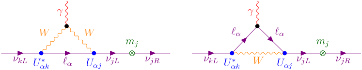
Figure 2: Feynman diagrams illustrating the proportionality of the magnetic moments to the neutrino masses, which are required to flip the neutrino chirality through the mass terms $m_{j}\overline{\nu_{jR}}\nu_{jL}$.

In the case of Majorana neutrinos the right-handed fields $\nu_{jR}$ in Eq.19 are replaced by $\nu_{jL}^{c}$:

$$\mathcal{L}_{\text{mag}}^{\text{M}}=-\dfrac{1}{4}\sum_{k,j}\overline{\nu_{kL}}\,\sigma^{\alpha\beta}\mu_{kj}^{\text{M}}\nu_{jL}^{c}\,F_{\alpha\beta}+\text{h.c.},$$ (24)

with an additional factor $1/2$ to avoid double counting. In the minimal extension of the SM with Majorana neutrino masses it is necessary to have a Majorana mass contribution in order to flip the chirality ($\nu_{jL}^{c}$ is right-handed) and the magnetic moments are again proportional to the neutrino masses [41]. Since the Lagrangian 24 is antisymmetric with respect to the neutrino mass indices, Majorana neutrinos can have only imaginary transition magnetic moments (in agreement with Eq.11). They are as suppressed as the Dirac transition magnetic moments in the minimal extension of the SM with Majorana neutrino masses [41]. However, in more elaborate models the Majorana magnetic moments can be enhanced by several orders of magnitude [40, 44, 45, 46, 47, 48].

In Tables 1 and 2 we present a list of the bounds on neutrino magnetic moments obtained from observations. They concern effective neutrino magnetic moments which are explained in the following. In any case, one can see that the current sensitivity is several orders of magnitude lower than that required to test the values in Eqs.21–23. Nevertheless, the bounds in Tables 1 and 2 are significant and it is important to develop new experiments with improved sensitivity in order to test non-minimal BSM models which predict large neutrino magnetic moments [16, 48].

Method	Experiment	Limit $[\mu_{\text{B}}]$	CL	Year	Ref.
Reactor $\bar{\nu}_{e}$ E$\nu$ES	Krasnoyarsk	$\mu_{\nu_{e}}<2.4\times 10^{-10}$	90%	1992	[49]
	Rovno	$\mu_{\nu_{e}}<1.9\times 10^{-10}$	95%	1993	[50]
	MUNU	$\mu_{\nu_{e}}<9\times 10^{-11}$	90%	2005	[51]
	TEXONO	$\mu_{\nu_{e}}<7.4\times 10^{-11}$	90%	2006	[52]
	GEMMA	$\mu_{\nu_{e}}<2.9\times 10^{-11}$	90%	2012	[53]
	CONUS	$\mu_{\nu_{e}}<7.5\times 10^{-11}$	90%	2022	[54]
Accelerator $\nu_{e}$ E$\nu$ES	LAMPF	$\mu_{\nu_{e}}<1.1\times 10^{-9}$	90%	1992	[55]
Accelerator $\nu_{\mu},\bar{\nu}_{\mu}$ E$\nu$ES	BNL-E734	$\mu_{\nu_{\mu}}<8.5\times 10^{-10}$	90%	1990	[56]
	LAMPF	$\mu_{\nu_{\mu}}<7.4\times 10^{-10}$	90%	1992	[55]
	LSND	$\mu_{\nu_{\mu}}<6.8\times 10^{-10}$	90%	2001	[57]
Accelerator $\nu_{\tau},\bar{\nu}_{\tau}$ E$\nu$ES	BEBC [58]	$\mu_{\nu_{\tau}}<5.4\times 10^{-7}$	90%	1991	[59]
	DONUT	$\mu_{\nu_{\tau}}<3.9\times 10^{-7}$	90%	2001	[60]
Accelerator $\nu_{e},\nu_{\mu},\bar{\nu}_{\mu}$ CE$\nu$NS+E$\nu$ES	COHERENT [61, 62]	$\begin{array}[]{c}\displaystyle\mu_{\nu_{e}}<4.2\times 10^{-9}\\[-2.84544pt] \displaystyle\mu_{\nu_{\mu}}<1.8\times 10^{-9}\end{array}$	90%	2022	[63, 64]
Reactor $\bar{\nu}_{e}$ CE$\nu$NS+E$\nu$ES	Dresden-II [65]	$\mu_{\nu_{e}}<2.1\times 10^{-10}$	90%	2022	[63, 64]
$e^{+}e^{-}\to\nu\bar{\nu}\gamma$ (Dirac $\nu$)	ASP, MAC, CELLO, MARK-J	$\mu_{\nu}<4\times 10^{-6}$	90%	1988	[66]
	TRISTAN	$\mu_{\nu}<8.0\times 10^{-6}$	90%	2000	[67]

Table 1: Limits for the neutrino magnetic moments obtained in laboratory short-baseline experiments. $\mu_{\nu}$ indicates a generic neutrino flavor.

Method	Experiment	Limit $[\mu_{\text{B}}]$	CL	Year	Ref.
Solar E$\nu$ES	Super-Kamiokande	$\mu_{\text{S}}^{\text{HE}}<1.1\times 10^{-10}$	90%	2004	[68]
	Borexino	$\begin{array}[]{c}\displaystyle\mu_{\text{S}}^{\text{LE}}<2.8\times 10^{-11}\\ \displaystyle\mu_{\nu_{e}}<3.9\times 10^{-11}\\ \displaystyle\mu_{\nu_{\mu}},\mu_{\nu_{\tau}}<5.8\times 10^{-11}\end{array}$	90%	2017	[69]
	XMASS-I	$\mu_{\text{S}}^{\text{LE}}<1.8\times 10^{-10}$	90%	2020	[70]
	XENONnT	$\mu_{\text{S}}^{\text{LE}}<6.4\times 10^{-12}$	90%	2022	[71]
	LUX-ZEPLIN	$\mu_{\text{S}}^{\text{LE}}<1.36\times 10^{-11}$	90%	2023	[72]
	PandaX-4T	$\mu_{\text{S}}^{\text{LE}}<2.2\times 10^{-11}$	90%	2024	[73]
	LUX-ZEPLIN [74]	$\begin{array}[]{c}\displaystyle\mu_{\text{S}}^{\text{LE}}<1.1\times 10^{-11}\\ \displaystyle\mu_{\nu_{e}}<1.5\times 10^{-11}\\ \displaystyle\mu_{\nu_{\mu}}<2.3\times 10^{-11}\\ \displaystyle\mu_{\nu_{\tau}}<2.1\times 10^{-11}\end{array}$	90%	2022	[75]
	XENONnT [71]	$\begin{array}[]{c}\displaystyle\mu_{\text{S}}^{\text{LE}}<6.3\times 10^{-12}\\ \displaystyle\mu_{\nu_{e}}<8.5\times 10^{-12}\\ \displaystyle\mu_{\nu_{\mu}}<1.4\times 10^{-11}\\ \displaystyle\mu_{\nu_{\tau}}<1.2\times 10^{-11}\end{array}$	90%	2022	[76]
	XENONnT [71]	$\begin{array}[]{c}\displaystyle\mu_{\nu_{e}}<9.0\times 10^{-12}\\ \displaystyle\mu_{\nu_{\mu}}<1.5\times 10^{-11}\\ \displaystyle\mu_{\nu_{\tau}}<1.3\times 10^{-11}\end{array}$	90%	2022	[77]
	LUX-ZEPLIN [74] $+$ PandaX-4T [78] $+$ XENONnT [71]	$\begin{array}[]{c}\displaystyle\mu_{\text{S}}^{\text{LE}}<7.5\times 10^{-12}\\ \displaystyle\mu_{\nu_{e}}<1.0\times 10^{-11}\\ \displaystyle\mu_{\nu_{\mu}},\mu_{\nu_{\tau}}<1.6\times 10^{-11}\end{array}$	90%	2023	[79]
Core-Collapse Supernovae		$\mu_{\nu}\lesssim(2-8)\times 10^{-12}$		1988	[80]
		$\mu_{\nu}\lesssim(1-4)\times 10^{-12}$		1998	[81, 82]
		$\mu_{\nu}\lesssim(1.1-2.7)\times 10^{-12}$		2009	[83]
Tip of the Red Giant Branch (TRGB)		$\mu_{\nu}\lesssim 3\times 10^{-12}$		1989	[84]
		$\mu_{\nu}\lesssim 1\times 10^{-12}$		1993	[85]
		$\mu_{\nu}<4.5\times 10^{-12}$	95%	2013	[86]
		$\mu_{\nu}\lesssim 2.6\times 10^{-12}$		2015	[87]
		$\mu_{\nu}<1.2\times 10^{-12}$	95%	2020	[88]
		$\mu_{\nu}\lesssim(1-5)\times 10^{-12}$		2020	[89]
		$\mu_{\nu}\lesssim 6\times 10^{-12}$		2023	[90]
Solar Cooling		$\mu_{\nu}\lesssim 4\times 10^{-10}$		1999	[91]
Cepheid Stars		$\mu_{\nu}\lesssim 2\times 10^{-10}$		2020	[92]
White Dwarfs		$\mu_{\nu}\lesssim(7-9)\times 10^{-12}$		2014	[93]
		$\mu_{\nu}<5\times 10^{-12}$	95%	2014	[94]
Big-Bang Nucleosynthesis (BBN)		$\mu_{\nu}\lesssim(1-2)\times 10^{-11}$		1981	[95]
		$\mu_{\nu}\lesssim 6.2\times 10^{-11}$		1997	[96]
		$\mu_{\nu}\lesssim 4\times 10^{-12}$		2023	[97]
Cosmological $N_{\text{eff}}$		$\mu_{\nu}<2.7\times 10^{-12}$	95%	2022	[98]
		$\mu_{\nu}<2.6\times 10^{-12}$	95%	2022	[99]
		$\mu_{\nu}<5\times 10^{-12}$	68%	2023	[97]

Table 2: Astrophysical limits for the neutrino magnetic moments. $\mu_{\text{S}}^{\text{LE}}$ and $\mu_{\text{S}}^{\text{HE}}$ are the low-energy and high-energy effective magnetic moments in solar neutrino experiments (see Eqs.40–42). $\mu_{\nu}$ indicates a generic neutrino flavor.

In laboratory experiments the effects of neutrino magnetic moments are searched through elastic neutrino-electron scattering (E$\nu$ES) or with coherent elastic neutrino-nucleus scattering (CE$\nu$NS). The latter method has become available only recently, after the observation of CE$\nu$NS in the COHERENT experiment [100, 61, 62].

Elastic neutrino-electron scattering of a flavor neutrino $\nu_{\ell}$ is the process

$$\nu_{\ell}+e^{-}\to\nu_{\ell^{\prime}}+e^{-}.$$ (25)

In the SM the neutrino flavor is conserved ($\ell^{\prime}=\ell$) and the E$\nu$ES cross section of a flavor neutrino $\nu_{\ell}$ with an electron bound in an atom $\mathcal{A}$ is given by

$$\dfrac{d\sigma_{\nu_{\ell}-\mathcal{A}}^{\text{E$\nu$ES},\text{SM}}}{dT_{\text{e}}}(E_{\nu},T_{\text{e}})=Z_{\text{eff}}^{\mathcal{A}}(T_{e})\,\dfrac{G_{\text{F}}^{2}m_{e}}{2\pi}\left[\left(g_{V}^{\nu_{\ell}}+g_{A}^{\nu_{\ell}}\right)^{2}+\left(g_{V}^{\nu_{\ell}}-g_{A}^{\nu_{\ell}}\right)^{2}\left(1-\dfrac{T_{e}}{E_{\nu}}\right)^{2}-\left((g_{V}^{\nu_{\ell}})^{2}-(g_{A}^{\nu_{\ell}})^{2}\right)\dfrac{m_{e}T_{e}}{E_{\nu}^{2}}\right],$$ (26)

where $G_{\text{F}}$ is the Fermi constant, $m_{e}$ is the electron mass, $E_{\nu}$ is the neutrino energy, and $T_{e}$ is the observable electron recoil energy. The neutrino-electron couplings $g_{V,A}^{\nu_{\ell}}$ depend on the neutrino flavor [75]:

$$g_{V}^{\nu_{e}}=\hbox{} \hbox{}2\sin^{2}\vartheta_{W}+1/2+\text{r.c.}=0.9521,\hbox{} \hbox{}g_{A}^{\nu_{e}}=\hbox{} \hbox{}1/2+\text{r.c.}=0.4938,$$ (27)

$$g_{V}^{\nu_{\mu}}=\hbox{} \hbox{}2\sin^{2}\vartheta_{W}-1/2+\text{r.c.}=-0.0397,\hbox{} \hbox{}g_{A}^{\nu_{\mu}}=\hbox{} \hbox{}-1/2+\text{r.c.}=-0.5062,$$ (28)

$$g_{V}^{\nu_{\tau}}=\hbox{} \hbox{}2\sin^{2}\vartheta_{W}-1/2+\text{r.c.}=-0.0353,\hbox{} \hbox{}g_{A}^{\nu_{\tau}}=\hbox{} \hbox{}-1/2+\text{r.c.}=-0.5062,$$ (29)

where $\sin^{2}\vartheta_{W}=0.23873\pm 0.00005$ [1] is the weak mixing angle and “r.c.” are radiative corrections. The coefficient $Z_{\text{eff}}^{\mathcal{A}}(T_{e})$ quantifies the effective number of electrons which can be ionized at $T_{e}$ [101] (see also Refs.102, 63, 64, 75). For antineutrinos the sign of $g_{A}^{\nu_{\ell}}$ must be changed.

Coherent neutrino-nucleus scattering is the process (see, e.g., the reviews 20, 104)

$$\nu_{\ell}+{}^{A}_{Z}\mathcal{N}\to\nu_{\ell^{\prime}}+{}^{A}_{Z}\mathcal{N},$$ (30)

with a coherent interaction of the neutrino with the nucleus, such that the nucleus recoils as a whole, without any change in its internal structure. This process was predicted theoretically in 1973 [105], but it was observed experimentally for the first time only in 2017 by the COHERENT experiment [100], because the only observable is the recoil of the nucleus with an extremely small kinetic energy which can be measured only with recently-developed very sensitive detectors [106]. The CE$\nu$NS cross-section of $\nu_{\ell}$ with a nucleus ${}^{A}_{Z}\mathcal{N}$ with $Z$ protons and $N=A-Z$ neutrons is given by

$$\dfrac{d\sigma_{\nu_{\ell}\mathcal{N}}^{\text{CE$\nu$NS}}}{dT_{\mathcal{N}}}(E_{\nu},T_{\mathcal{N}})=\dfrac{G_{\text{F}}^{2}M_{\mathcal{N}}}{\pi}\left(1-\dfrac{M_{\mathcal{N}}T_{\mathcal{N}}}{2E_{\nu}^{2}}-\dfrac{T_{\mathcal{N}}}{E_{\nu}}\right)\left[Q_{\nu_{\ell}\mathcal{N}}(|\hskip-1.0pt\vec{\hskip 1.0ptq}|)\right]^{2},$$ (31)

where $T_{\mathcal{N}}$ is the kinetic recoil energy of the nucleus, $M_{\mathcal{N}}$ is the nuclear mass, $Q_{\nu_{\ell}\mathcal{N}}(|\hskip-1.0pt\vec{\hskip 1.0ptq}|)$ is the charge of the nucleus for the interactions which contribute to CE$\nu$NS, and $|\hskip-1.0pt\vec{\hskip 1.0ptq}|\simeq\sqrt{2M_{\mathcal{N}}T_{\mathcal{N}}}$ is the absolute value of the three-momentum transferred from the neutrino to the nucleus. In the SM CE$\nu$NS is a weak neutral current interaction process mediated by the $Z^{0}$ neutral boson, $\ell^{\prime}=\ell$, and

$$Q_{\nu_{\ell}\mathcal{N}}^{\text{SM}}(|\hskip-1.0pt\vec{\hskip 1.0ptq}|)=g_{V}^{n}\,N\,F_{N}^{\mathcal{N}}(|\hskip-1.0pt\vec{\hskip 1.0ptq}|)+g_{V}^{p}(\nu_{\ell})\,Z\,F_{Z}^{\mathcal{N}}(|\hskip-1.0pt\vec{\hskip 1.0ptq}|)$$ (32)

is called “weak charge of the nucleus”. The functions $F_{N}^{\mathcal{N}}(|\hskip-1.0pt\vec{\hskip 1.0ptq}|)$ and $F_{Z}^{\mathcal{N}}(|\hskip-1.0pt\vec{\hskip 1.0ptq}|)$ are, respectively, the neutron and proton form factors of the nucleus ${}^{A}_{Z}\mathcal{N}$, which are the Fourier transforms of the neutron and proton distributions in the nucleus and characterize the amount of coherency of the interaction. The coefficients $g_{V}^{n}$ and $g_{V}^{p}$ are given by [108]

$$g_{V}^{n}=-\frac{1}{2}+\text{r.c.}=-0.5117\quad\text{and}\quad g_{V}^{p}(\nu_{\ell})=\dfrac{1}{2}-2\sin^{2}\!\vartheta_{W}+\text{r.c.}=\left\{\begin{array}[]{l}\displaystyle 0.0382\quad\text{for}\quad\nu_{e},\\ \displaystyle 0.0300\quad\text{for}\quad\nu_{\mu},\\ \displaystyle 0.0256\quad\text{for}\quad\nu_{\tau}.\end{array}\right.$$ (33)

Therefore, taking also into account that in typical CE$\nu$NS heavy nuclear targets $N>Z$, the neutron contribution is much larger than the proton contribution and the SM CE$\nu$NS cross section is approximately proportional to the square of the neutron number $N$ of the nucleus.

The cross section of the elastic scattering of neutrinos with a target particle due to an effective neutrino magnetic moment $\mu_{\nu}$ (discussed in the following) is given by

$$\frac{d\sigma(\mu_{\nu})}{dT}=C\,\frac{\pi\alpha^{2}}{m_{e}^{2}}\left(\frac{1}{T}-\frac{1}{E_{\nu}}\right)\frac{\mu_{\nu}^{2}}{\mu_{\text{B}}^{2}},$$ (34)

where $\alpha$ is the fine-structure constant, $T$ is the observable kinetic energy of the recoil target particle, and $C$ is a coefficient which depends on the target particle: $C=1$ and $T=T_{e}$ for elastic scattering with a free electron; $C=Z_{\text{eff}}^{\mathcal{A}}(T_{e})$ and $T=T_{e}$ for elastic scattering with an electron bound in an atom $\mathcal{A}$; $C=Z^{2}[F_{Z}^{\mathcal{N}}(|\hskip-1.0pt\vec{\hskip 1.0ptq}|)]^{2}$ and $T=T_{\mathcal{N}}$ in CE$\nu$NS with a nucleus with atomic number $Z$.

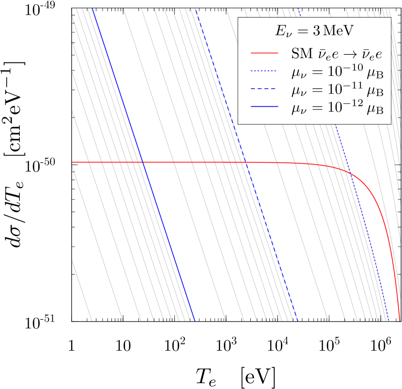
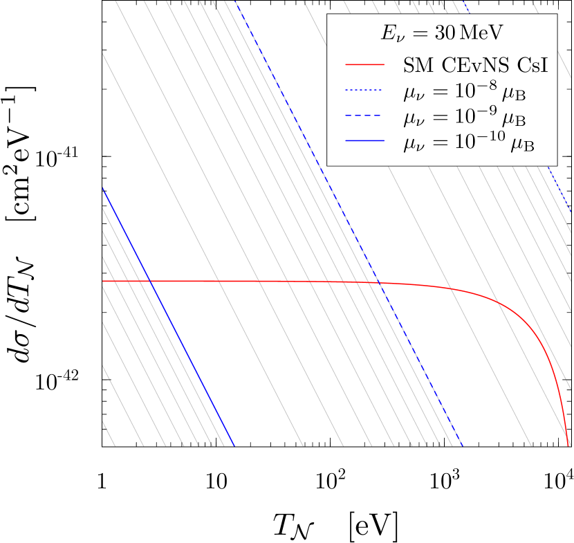
Figure 3: Differential cross sections for elastic neutrino-electron scattering (E$\nu$ES, left) and coherent neutrino-nucleus scattering (CE$\nu$NS, right) as functions of the observable kinetic energy of the recoil target particle. For E$\nu$ES the value of the neutrino energy $E_{\nu}$ is typical of reactor neutrino experiments, whereas for CE$\nu$NS it is typical of neutrinos produced by pion decay at rest, as in the COHERENT experiment [100]. For CE$\nu$NS the cross sections are the average cross sections for ${}^{133}\text{Cs}$ and ${}^{127}\text{I}$, which constitute the COHERENT CsI detector [100].

Since the magnetic moment interaction flips the helicity of ultrarelativistic neutrinos, it is not coherent with the SM weak interaction and the total cross section of a scattering process is the sum of the two cross sections. As shown in Fig.3, the magnetic moment cross section can be larger than the weak cross section for low values of $T$, because of its approximate $1/T$ dependence. When this happens it distorts the energy spectrum of the recoil target particle, giving information on the value of the magnetic moment. From Fig.3 one can see that both E$\nu$ES and CE$\nu$NS are sensitive to the neutrino magnetic moment, but E$\nu$ES of reactor neutrinos can probe smaller values of $\mu_{\nu}$ than CE$\nu$NS in the COHERENT experiment. Indeed, one can see from Table 1 that E$\nu$ES experiments with reactor $\bar{\nu}_{e}$’s have obtained bounds on the effective $\mu_{\nu_{e}}$ which are better than the COHERENT bound (for which a small E$\nu$ES contribution, which is indistinguishable from the main CE$\nu$NS signal in the COHERENT detector, has been taken into account). The most stringent bound on $\mu_{\nu_{e}}$ has been obtained by the GEMMA [53] experiment from E$\nu$ES of reactor $\bar{\nu}_{e}$’s at the Kalinin Nuclear Power Plant in Russia, with a 1.5 kg high-purity germanium (HPGe) detector with an energy threshold of 2.8 keV. On the other hand, since the neutrino beam in the COHERENT experiment includes $\nu_{\mu}$’s and $\bar{\nu}_{\mu}$’s, the COHERENT data constrain also $\mu_{\nu_{\mu}}$. From Table 1, one can see that the CE$\nu$NS +E$\nu$ES COHERENT bound on $\mu_{\nu_{\mu}}$ is not far from the more stringent bounds obtained in accelerator E$\nu$ES experiments.

In Table 1 we report also generic limits on the neutrino magnetic moments obtained from searches of $e^{+}e^{-}\to\nu\bar{\nu}\gamma$ events in high-energy experiments neglecting a possible $q^{2}$ dependence of the magnetic form factor.

The magnetic moment in Eq.34 is an effective magnetic moment [109, 110] which depends on the experiment under consideration and is given, in general, by

$$\mu_{\nu}^{2}=\sum_{j}\left|\sum_{k}\mu_{jk}A_{k}(E_{\nu},L)\right|^{2},$$ (35)

where $A_{k}(E_{\nu},L)$ is the amplitude of the massive neutrino $\nu_{k}$ with energy $E_{\nu}$ after propagation over a source-detector distance $L$. The contributions of the detected initial massive neutrinos in the interaction process, labeled with the index $k$, are summed coherently, whereas the contributions of the undetected final massive neutrinos in the interaction process, labeled with the index $j$, are summed incoherently.

For neutrino propagation in vacuum $A_{k}(E_{\nu},L)=A_{k}^{0}(E_{\nu})e^{-im_{k}^{2}L/2E_{\nu}}$, where $A_{k}^{0}(E_{\nu})$ is the amplitude of $\nu_{k}$ production at the source and $e^{-im_{k}^{2}L/2E_{\nu}}$ is the phase of $\nu_{k}$. If the source emits a $\nu_{\ell}$ or $\bar{\nu}_{\ell}$ flux in matter with a normal density $A_{k}^{0}\simeq U_{\ell k}^{*}$ or $A_{k}^{0}\simeq U_{\ell k}$, respectively.

In short-baseline experiments with neutrinos from reactors and accelerators, the neutrino source-detector distance is shorter than the oscillation length ($L\ll 4\pi E_{\nu}/\Delta{m}^{2}_{kj}$) and the detected neutrino flavor is the same as the flavor of the neutrino emitted by the source (e.g. $\bar{\nu}_{e}$ for reactor neutrinos). In this case, $A_{k}\simeq U_{\ell k}^{*}$ if the source emits a $\nu_{\ell}$ flux, and $A_{k}\simeq U_{\ell k}$ if the source emits a $\bar{\nu}_{\ell}$ flux. Therefore, taking into account the property 9, the squared effective magnetic moments of $\nu_{\ell}$ and $\bar{\nu}_{\ell}$ are equally given by

$$\mu_{\nu_{\ell}}^{2}\simeq\mu_{\bar{\nu}_{\ell}}^{2}\simeq\sum_{j}\left|\sum_{k}\mu_{jk}U_{\ell k}^{*}\right|^{2}=\sum_{\ell^{\prime}}\left|\mu_{\ell^{\prime}\ell}\right|^{2}=\mu_{\ell\ell}^{2}+\sum_{\ell^{\prime}\neq\ell}\left|\mu_{\ell\ell^{\prime}}\right|^{2},$$ (36)

where $\mu_{\ell^{\prime}\ell}=\mu_{\ell\ell^{\prime}}^{*}$ are the flavor magnetic moments given by the transformation 17:

$$\mu_{\ell^{\prime}\ell}=\sum_{j,k}U_{\ell^{\prime}j}\mu_{jk}U_{\ell k}^{*}.$$ (37)

Therefore, the squared effective magnetic moment that is measured in a $\nu_{\ell}$ short-baseline experiment is given by the sum of the squared diagonal magnetic moment $\mu_{\ell\ell}$ of $\nu_{\ell}$ and the squared absolute values of the transition magnetic moments $\mu_{\ell\ell^{\prime}}$ for $\ell^{\prime}\neq\ell$. The same result could have been obtained in the flavor basis summing incoherently over the possible flavors $\ell^{\prime}$ of the undetected final neutrino $\nu_{\ell^{\prime}}$ (see Eqs.25 and 30):

$$\mu_{\nu}^{2}=\sum_{\ell^{\prime}}\left|\sum_{\ell^{\prime\prime}}\mu_{\ell^{\prime}\ell^{\prime\prime}}A_{\ell^{\prime\prime}}(E_{\nu},L)\right|^{2}.$$ (38)

In a short-baseline experiment with a $\nu_{\ell}$ or $\bar{\nu}_{\ell}$ source, $A_{\ell^{\prime\prime}}(E_{\nu},L)=\delta_{\ell\ell^{\prime\prime}}$ and Eq.38 gives Eq.36.

The effective flavor magnetic moments $\mu_{\nu_{\ell}}$ in Table 1 which are bounded by short-baseline reactor and accelerator neutrino experiments are given by the square root of Eq.36. Therefore they constrain not only the diagonal magnetic moment $\mu_{\ell\ell}$ of $\nu_{\ell}$, but also the transition magnetic moments $\mu_{\ell\ell^{\prime}}$ for $\ell^{\prime}\neq\ell$.

If the neutrino source and detector are far away, the detected neutrino flux may contain flavor neutrinos which are different from the initial one and it is convenient to consider the expression 38 of $\mu_{\nu}^{2}$ in the flavor basis. In the case of solar neutrinos, $L$ is very large and the interference terms in Eq.38 are washed out by the neutrino energy spectrum, leading to the effective magnetic moment

$$\mu_{\text{S}}^{2}\simeq\sum_{\ell}P^{\text{S}}_{e\ell}(E_{\nu})\sum_{\ell^{\prime}}\left|\mu_{\ell^{\prime}\ell}\right|^{2},$$ (39)

where $P^{\text{S}}_{e\ell}(E_{\nu})$ is the probability of solar $\nu_{e}\to\nu_{\ell}$ transitions. Taking into account that $P^{\text{S}}_{e\mu}=\cos^{2}\vartheta_{23}\left(1-P^{\text{S}}_{ee}\right)$ and $P^{\text{S}}_{e\tau}=\sin^{2}\vartheta_{23}\left(1-P^{\text{S}}_{ee}\right)$, Eq.39 can be written as

$$\mu_{\text{S}}^{2}=P^{\text{S}}_{ee}\,\mu_{\nu_{e}}^{2}+\left(1-P^{\text{S}}_{ee}\right)\left(\cos^{2}\vartheta_{23}\,\mu_{\nu_{\mu}}^{2}+\sin^{2}\vartheta_{23}\,\mu_{\nu_{\tau}}^{2}\right).$$ (40)

with $\mu_{\nu_{e}}$, $\mu_{\nu_{\mu}}$, and $\mu_{\nu_{\tau}}$ given by Eq.36. For low-energy and high-energy solar neutrinos

$$P^{\text{S}}_{ee}\simeq\left(1-\frac{1}{2}\,\sin^{2}2\vartheta_{12}\right)\cos^{4}\vartheta_{13}+\sin^{4}\vartheta_{13}=P^{\text{S,LE}}_{ee} \quad\text{for}\quad E_{\nu}\lesssim 1\,\text{MeV},$$ (41)

$$P^{\text{S}}_{ee}\simeq\sin^{2}\vartheta_{12}\cos^{4}\vartheta_{13}+\sin^{4}\vartheta_{13}=P^{\text{S,HE}}_{ee} \quad\text{for}\quad E_{\nu}\gtrsim 5\,\text{MeV}.$$ (42)

Using the values of the mixing angles in Eq.3, we obtain $P^{\text{S,LE}}_{ee}=0.542\pm 0.011$ and $P^{\text{S,HE}}_{ee}=0.305\pm 0.015$ independently of the ordering of the neutrino masses. Therefore, the effective solar neutrino magnetic moment obtained from the analyses of the data of low-energy ($\mu_{\text{S}}^{\text{LE}}$) and high-energy ($\mu_{\text{S}}^{\text{HE}}$) solar neutrino experiments are different and cannot be compared directly. The results on the measurement of the effective solar neutrino magnetic moment can be compared directly only among solar neutrino experiments which detect neutrinos with the same energy range, as those for $\mu_{\text{S}}^{\text{LE}}$ in Table 2. The results on $\mu_{\nu_{e}}$, $\mu_{\nu_{\mu}}$, and $\mu_{\nu_{\tau}}$ can be compared with the caveat that they may have been obtained with slightly different values of $P^{\text{S}}_{ee}$ and $\vartheta_{23}$ and different treatments of the systematic uncertainties. In any case, one can see from Table 2 that the best solar bounds on $\mu_{\nu_{e}}$ and all the solar bounds on $\mu_{\nu_{\mu}}$ and $\mu_{\nu_{\tau}}$ are stronger than those of reactors and accelerators in Table 1.

In Table 2 we listed also astrophysical bounds which have larger systematic uncertainties and are less accurate than the previous bounds. Nevertheless, it is useful to have a view of them, because it is an active field of research and they are quite stringent. Since these limits have been obtained without taking into account neutrino mixing, they apply approximately to all neutrino flavors. The Core-Collapse Supernovae bounds stem from the limit on a possible energy loss due to scattering processes which induce magnetic moment transitions from left-handed neutrinos to sterile right-handed neutrinos which escape from the environment. The TRGB, Solar Cooling, Cepheid Stars, and White Dwarfs bounds ensue from the energy loss due to plasmon decay into a neutrino-antineutrino pair [14] discussed in Section 7.3. The BBN (Big Bang Nucleosynthesis) and $N_{\text{eff}}$ bounds follow from the constraints on the production of right-handed neutrinos by the scattering of left-handed neutrinos with a magnetic moment with the charged particles in the primordial plasma. In the calculations of Ref.[99] the bound on the neutrino magnetic moment depends on the assumed value $T_{\text{in}}$ of the temperature of the Universe at which the production of right-handed neutrino starts. The bound $\mu_{\nu}<2.6\times 10^{-12}$ at 95% CL reported in Table 2 was obtained assuming $T_{\text{in}}=100\,\text{GeV}$ and is in approximate agreement with those of Refs.[98, 97], also reported in Table 2. Assuming a smaller initial temperature the limit becomes less stringent, since less right-handed neutrino are produced (e.g., for $T_{\text{in}}=100\,\text{MeV}$, the bound becomes $\mu_{\nu}<1.6\times 10^{-11}$ at 95% CL). Future possibilities to measure very small neutrino magnetic moments with astrophysical neutrinos have been discussed in Refs.[111, 112].

5 Neutrino charge radius

The neutrino charge radii describe virtual charge distributions which can exist even if the neutrinos are neutral. They are given by the first-order $q^{2}$ dependence of the charge form factors in Eq.13. Therefore, they are phenomenological quantities which can be measured in neutrino scattering with charged particles, as E$\nu$ES and CE$\nu$NS.

Theoretically, the neutrino charge radii are generated by radiative corrections and exist even in the SM, where neutrinos are neutral and massless [29, 30, 31, 32]. Since in the SM the generation lepton numbers are conserved, the SM charge radii are defined in the flavor basis. Taking into account one-loop radiative corrections, they are given by [31]

$$\langle r_{\nu_{\ell}}^{2}\rangle^{\text{SM}}=-\frac{G_{\text{F}}}{2\sqrt{2}\pi^{2}}\left[3-2\ln\left(\frac{m_{\ell}^{2}}{m^{2}_{W}}\right)\right]=\left\{\begin{array}[]{rl}\displaystyle-0.83\times 10^{-32}\,\text{cm}^{2}&\displaystyle(\nu_{e})\\ \displaystyle-0.48\times 10^{-32}\,\text{cm}^{2}&\displaystyle(\nu_{\mu})\\ \displaystyle-0.30\times 10^{-32}\,\text{cm}^{2}&\displaystyle(\nu_{\tau})\end{array}\right.$$ (43)

where $m_{W}$ is the $W$ boson mass and $m_{\ell}$ are the charged lepton masses for $\ell=e,\mu,\tau$.

Finding deviations of the neutrino charge radii from the SM values would be a discovery of new BSM physics. Therefore, we consider the general case of diagonal and off-diagonal (transition) charge radii in the flavor basis, which are given, from Eq.17, by

$$\langle r_{\nu_{\ell^{\prime}\ell}}^{2}\rangle=\sum_{k,j}U_{\ell^{\prime}k}\langle r_{\nu_{kj}}^{2}\rangle U_{\ell j}^{*}.$$ (44)

As already noted after Eq.17, the unitary transformation from the mass to the flavor basis preserves the hermiticity of the matrix of charge radii: $\langle r_{\nu_{\ell^{\prime}\ell}}^{2}\rangle=\langle r_{\nu_{\ell\ell^{\prime}}}^{2}\rangle^{*}$. Hence, the diagonal charge radii of flavor neutrinos $\langle r_{\nu_{e}}^{2}\rangle\equiv\langle r_{\nu_{ee}}^{2}\rangle$, $\langle r_{\nu_{\mu}}^{2}\rangle\equiv\langle r_{\nu_{\mu\mu}}^{2}\rangle$, and $\langle r_{\nu_{\tau}}^{2}\rangle\equiv\langle r_{\nu_{\tau\tau}}^{2}\rangle$ are real.

The traditional way to obtain limits on $\langle r_{\nu_{e}}^{2}\rangle$ is the observation of elastic neutrino-electron scattering (E$\nu$ES) using the intense fluxes of reactor $\bar{\nu}_{e}$’s. The limits on $\langle r_{\nu_{\mu}}^{2}\rangle$ have been obtained with E$\nu$ES of accelerator $\nu_{\mu}$’s produced mainly by pion decay. These methods have been recently complemented by the measurement of coherent elastic neutrino-nucleus scattering (CE$\nu$NS) of low-energy electron and muon neutrinos produced by pion and muon decays at rest or reactor $\bar{\nu}_{e}$’s.

The total E$\nu$ES cross section of a flavor neutrino $\nu_{\ell}$ with an electron bound in an atom $\mathcal{A}$ is given by [114]

$$\dfrac{d\sigma_{\nu_{\ell}-\mathcal{A}}^{\text{E$\nu$ES},\text{SM+CR}}}{dT_{\text{e}}}=\left(\dfrac{d\sigma_{\nu_{\ell}-\mathcal{A}}^{\text{E$\nu$ES},\text{SM+CR}}}{dT_{\text{e}}}\right)_{\langle{r}_{\nu_{\ell}}^{2}\rangle}+\sum_{\ell^{\prime}\neq\ell}\left(\dfrac{d\sigma_{\nu_{\ell}-\mathcal{A}}^{\text{E$\nu$ES},\text{CR}}}{dT_{\text{e}}}\right)_{\langle{r}_{\nu_{\ell\ell^{\prime}}}^{2}\rangle}.$$ (45)

The first term takes into account coherently the effects of the SM weak interaction and the diagonal flavor-conserving neutrino charge radii. It is obtained from Eq.26 with the substitution

$$g_{V}^{\nu_{\ell}}\to g_{V}^{\nu_{\ell}}+\dfrac{\sqrt{2}\pi\alpha}{3G_{\text{F}}}\left(\langle{r}_{\nu_{\ell}}^{2}\rangle-\langle{r}_{\nu_{\ell}}^{2}\rangle^{\text{SM}}\right)=\left\{\begin{array}[]{l}\displaystyle\tilde{g}_{V}^{\nu_{e}}+\dfrac{\sqrt{2}\pi\alpha}{3G_{\text{F}}}\,\langle{r}_{\nu_{e}}^{2}\rangle\quad\text{for}\quad\ell=e,\\ \displaystyle\tilde{g}_{V}^{\nu_{\mu}}+\dfrac{\sqrt{2}\pi\alpha}{3G_{\text{F}}}\,\langle{r}_{\nu_{\ell}}^{2}\rangle\quad\text{for}\quad\ell=\mu,\tau,\end{array}\right.$$ (46)

where $\tilde{g}_{V}^{\nu_{\mu}}=-0.028$ and $\tilde{g}_{V}^{\nu_{e}}=\tilde{g}_{V}^{\nu_{\mu}}+1=0.972$. Since we are interested in the measurement of the neutrino charge radii including the SM contributions in Eq.43, we subtracted from the SM values of $g_{V}^{\nu_{\ell}}$ given by Eqs.27–29 the contributions of the SM charge radii which are included in the SM radiative corrections. Note that $\nu_{\ell}$ E$\nu$ES experiments are sensitive to the sign of the diagonal charge radius $\langle{r}_{\nu_{\ell}}^{2}\rangle=\langle{r}_{\nu_{\ell\ell}}^{2}\rangle$. The second term in Eq.45 takes into account the incoherent contribution of the transition charge radii:

$$\left(\dfrac{d\sigma_{\nu_{\ell}-\mathcal{A}}^{\text{E$\nu$ES},\text{CR}}}{dT_{\text{e}}}\right)_{\langle{r}_{\nu_{\ell\ell^{\prime}}}^{2}\rangle}=Z_{\text{eff}}^{\mathcal{A}}(T_{e})\,\dfrac{\pi\alpha^{2}m_{e}}{9}\left[1+\left(1-\dfrac{T_{e}}{E_{\nu}}\right)^{2}-\dfrac{m_{e}T_{e}}{E_{\nu}^{2}}\right]|\langle{r}_{\nu_{\ell\ell^{\prime}}}^{2}\rangle|^{2}\quad\text{for}\quad\ell^{\prime}\neq\ell.$$ (47)

Therefore, E$\nu$ES experiments with a pure $\nu_{\ell}$ beam are sensitive only to the sum of the squared absolute values of the transition charge radii $\langle{r}_{\nu_{\ell\ell^{\prime}}}^{2}\rangle$ for $\ell^{\prime}\neq\ell$ [114].

Method	Experiment	Limit $[10^{-32}\,\text{cm}^{2}]$	CL	Year	Ref.
Reactor $\bar{\nu}_{e}$ E$\nu$ES	Krasnoyarsk	$|\langle r_{\nu_{e}}^{2}\rangle|<7.3$	90%	1992	[49]
	TEXONO	$\langle r_{\nu_{e}}^{2}\rangle\in(-4.2,6.6)$	90%	2009	[115]
Accelerator $\nu_{e}$ E$\nu$ES	LAMPF	$\langle r_{\nu_{e}}^{2}\rangle\in(-7.12,10.88)$	90%	1992	[55] 13
	LSND	$\langle r_{\nu_{e}}^{2}\rangle\in(-5.94,8.28)$	90%	2001	[57] 13
$\nu_{\mu}$-nucleon DIS	NuTeV [116]	$|\langle r_{\nu_{\mu}}^{2}\rangle|<0.71$	90%	2002	[117]
Accelerator $\nu_{\mu}$ E$\nu$ES	BNL-E734 [56]	$\langle r_{\nu_{\mu}}^{2}\rangle\in(-1.1,5.7)$	90%	2002	[117]
	CHARM-II [118]	$\langle r_{\nu_{\mu}}^{2}\rangle\in(-2.2,0.52)$	90%	2002	[117] 14
	CCFR [119]	$\langle r_{\nu_{\mu}}^{2}\rangle\in(-0.68,0.53)$	90%	2002	[117] 14
Accelerator $\nu_{e},\nu_{\mu},\bar{\nu}_{\mu}$ $+$ Reactor $\bar{\nu}_{e}$ CE$\nu$NS	COHERENT [61, 62] $+$ Dresden-II [65]	$\begin{array}[]{c}\displaystyle\langle r_{\nu_{e}}^{2}\rangle\in(-7.1,5)\\ \displaystyle\langle r_{\nu_{\mu}}^{2}\rangle\in(-5.9,4.3)\end{array}$	90%	2022	[64]
Solar E$\nu$ES	XENONnT [71]	$\begin{array}[]{c}\displaystyle\langle r_{\nu_{e}}^{2}\rangle\in(-85,2.0)\\ \displaystyle\langle r_{\nu_{\mu}}^{2}\rangle\in(-45,52)\\ \displaystyle\langle r_{\nu_{\tau}}^{2}\rangle\in(-40,45)\end{array}$	90%	2022	[76]
	XENONnT [71]	$\begin{array}[]{c}\displaystyle\langle r_{\nu_{e}}^{2}\rangle\in(-93.4,9.5)\\ \displaystyle\langle r_{\nu_{\mu}}^{2}\rangle\in(-50.2,54)\\ \displaystyle\langle r_{\nu_{\tau}}^{2}\rangle\in(-43,46.8)\end{array}$	90%	2022	[77]
	LUX-ZEPLIN [74] $+$ PandaX-4T [78] $+$ XENONnT [71]	$\begin{array}[]{c}\displaystyle\langle r_{\nu_{e}}^{2}\rangle\in(-99.5,12.8)\\ \displaystyle\langle r_{\nu_{\mu}}^{2}\rangle,\langle r_{\nu_{\tau}}^{2}\rangle\in(-82.2,88.7)\end{array}$	90%	2023	[79]
$e^{+}e^{-}\to\nu\bar{\nu}\gamma$ (Dirac $\nu$)	ASP, MAC, CELLO, MARK-J	$|\langle r_{\nu}^{2}\rangle|<20$	90%	1988	[66]
	TRISTAN	$\langle r_{\nu}^{2}\rangle\in(-18,21)$	90%	2002	[117] 14
	LEP-2	$\langle r_{\nu}^{2}\rangle\in(-6.2,5.6)$	90%	2002	[117] 14
$e^{+}e^{-}\to\nu\bar{\nu}\gamma$ (Majorana $\nu$)	TRISTAN	$\langle r_{\nu}^{2}\rangle\in(-31,37)$	90%	2002	[117] 14
	LEP-2	$\langle r_{\nu}^{2}\rangle\in(-9.9,8.2)$	90%	2002	[117] 14
BBN (Dirac $\nu$)		$|\langle r_{\nu}^{2}\rangle|\lesssim 0.7$		1987	[120]
SN1987A (Dirac $\nu$)		$|\langle r_{\nu}^{2}\rangle|\lesssim 0.2$		1989	[121]
TRGB		$|\langle r_{\nu}^{2}\rangle|\lesssim 40-50$		1994	[122]

Table 3: Limits for the charge radii of flavor neutrinos obtained assuming the absence of transition charge radii. These limits can be compared with the Standard Model predictions in Eq.43. $\langle r_{\nu}^{2}\rangle$ indicates a generic neutrino flavor.

The CE$\nu$NS cross section of a flavor neutrino $\nu_{\ell}$ with a nucleus ${}^{A}_{Z}\mathcal{N}$ is given by Eq.31 with

$$\left|Q_{\nu_{\ell}\mathcal{N}}^{\text{SM+CR}}(|\hskip-1.0pt\vec{\hskip 1.0ptq}|)\right|^{2}=\left[g_{V}^{n}\,N\,F_{N}^{\mathcal{N}}(|\hskip-1.0pt\vec{\hskip 1.0ptq}|)+\left(\tilde{g}_{V}^{p}-\widetilde{Q}_{\ell\ell}\right)Z\,F_{Z}^{\mathcal{N}}(|\hskip-1.0pt\vec{\hskip 1.0ptq}|)\right]^{2}+\left[Z\,F_{Z}^{\mathcal{N}}(|\hskip-1.0pt\vec{\hskip 1.0ptq}|)\right]^{2}\sum_{\ell^{\prime}\neq\ell}|\widetilde{Q}_{\ell\ell^{\prime}}|^{2},$$ (48)

where $\tilde{g}_{V}^{p}=0.0186$ is the neutrino-proton coupling without the contribution of the SM neutrino charge radius, which is included in the radiative corrections in Eq.33. The effects of the charge radii $\langle{r}_{\nu_{\ell\ell^{\prime}}}^{2}\rangle$ are given by

$$\widetilde{Q}_{\ell\ell^{\prime}}=\dfrac{\sqrt{2}\pi\alpha}{3G_{\text{F}}}\,\langle{r}_{\nu_{\ell\ell^{\prime}}}^{2}\rangle.$$ (49)

As in the case of E$\nu$ES, the contribution of the diagonal charge radius $\langle{r}_{\nu_{\ell}}^{2}\rangle=\langle{r}_{\nu_{\ell\ell}}^{2}\rangle$ is added coherently to the SM weak interaction and $\nu_{\ell}$ CE$\nu$NS experiments are sensitive to its sign. The contributions of the transition charge radii $\langle{r}_{\nu_{\ell\ell^{\prime}}}^{2}\rangle$ (for $\ell^{\prime}\neq\ell$) are added incoherently and $\nu_{\ell}$ CE$\nu$NS experiments are sensitive only to the sum of their squared absolute values, as $\nu_{\ell}$ E$\nu$ES experiments.

Experiments which have beams of different neutrino flavors with different characteristics (as the energy spectrum) can distinguish the contributions of the different diagonal charge radii and those of the different transition radii. This happens in the COHERENT experiment which has $\nu_{e}$, $\nu_{\mu}$, and $\bar{\nu}_{\mu}$, beams with different energy and time distributions. Since $|\langle{r}_{\nu_{e\mu}}^{2}\rangle|=|\langle{r}_{\nu_{\mu e}}^{2}\rangle|$ contributes to all events, $\langle{r}_{\nu_{e\tau}}^{2}\rangle$ contributes only to $\nu_{e}$-induced events, and $\langle{r}_{\nu_{\mu\tau}}^{2}\rangle$ contributes only to $\nu_{\mu}$ and $\bar{\nu}_{\mu}$-induced events, they can be distinguished. Solar neutrino experiments can distinguish all neutrino charge radii, because they detect different fluxes of $\nu_{e}$ and of $\nu_{\mu}$ and $\nu_{\tau}$ (if $\sin^{2}\vartheta_{23}\neq 0.5$).

However, the results of the analysis of the experimental data with all the diagonal and transition charge radii are complicated and suffer of degeneracies in the effects of the different charge radii. Most relevant is the possible cancellation of the contribution of a diagonal charge radius by the contribution of the corresponding transition charge radii. This can be seen clearly in CE$\nu$NS by noting that the main contribution to $\left|Q_{\nu_{\ell}\mathcal{N}}^{\text{SM+CR}}(|\hskip-1.0pt\vec{\hskip 1.0ptq}|)\right|^{2}$ in Eq.48 is due to $g_{V}^{n}$, which is negative (see Eq.33). A small negative value of $\langle{r}_{\nu_{\ell}}^{2}\rangle$ which increases the positive contribution of $\left(\tilde{g}_{V}^{p}-\widetilde{Q}_{\ell\ell}\right)$, leads to a decrease of the first part of $\left|Q_{\nu_{\ell}\mathcal{N}}^{\text{SM+CR}}(|\hskip-1.0pt\vec{\hskip 1.0ptq}|)\right|^{2}$ which can be compensated by increasing the second part with the transition charge radii.

Therefore, the analyses of the data without and with the transition charge radii can give rather different results. Moreover, as we have seen in Eq.43, the SM predicts the existence of only the diagonal flavor charge radii and it is plausible that the values of the transition charge radii generated by BSM physics are much smaller. Hence, in Table 3 we report the bounds on the diagonal charge radii of the flavor neutrinos obtained in different experiments and phenomenological analyses assuming the absence of the transition charge radii.

From Table 3 one can see that the most stringent bounds on $\langle r_{\nu_{e}}^{2}\rangle^{\text{SM}}$ and $\langle r_{\nu_{\mu}}^{2}\rangle^{\text{SM}}$ obtained in laboratory experiments are only about one order of magnitude larger than the SM predictions in Eq.43, and the CCFR bound on $\langle r_{\nu_{\mu}}^{2}\rangle^{\text{SM}}$ obtained in Ref.[117] is near the SM prediction. Therefore, an experimental effort is mandatory in order to try to improve the experimental sensitivity and try to discover the neutrino charge radii predicted by the SM.

In Table 3 we report also limits on the specific charge radii obtained in solar E$\nu$ES experiments, generic limits on the charge radii obtained from searches of $e^{+}e^{-}\to\nu\bar{\nu}\gamma$ events in high-energy TRISTAN and LEP-2 experiments, and generic limits on the charge radii obtained from BBN, SN1987A, and TRGB. Note that the BBN and SN1987A bounds are at the same level or smaller than the SM predictions, but the uncertainties are unknown.

The current bounds of solar neutrino experiments on all the neutrino charge radii are not competitive with the bounds obtained in laboratory experiments, but we must take into account that the results of solar low-energy E$\nu$ES are recent and come from experiments which have been constructed for the search of dark matter, in which solar neutrino interactions were considered as a background. Future dark matter and solar neutrino experiments, as DARWIN [124, 79], XLZD [125], and DarkSide [126], will reach higher sensitivities.

Accurate analyses of the data of future higher precision E$\nu$ES and CE$\nu$NS experiments will require to take into account the effects of the non-zero momentum transfer in the calculation of the neutrino charge radius radiative correction [123].

Method	Experiment	Limit $[e]$	CL	Year	Ref.
Neutrality of matter	K and Cs	$\mathcal{Q}_{\nu}=(-0.5\pm 3.5)\times 10^{-19}$	68%	1988	[127]
	$\text{SF}_{6}$ [128]	$\mathcal{Q}_{\nu}=(0.6\pm 3.2)\times 10^{-21}$	68%	2014	[16]
Magnetic Dichroism	PVLAS	$|Q_{\nu}|<3\times 10^{-8}$	95%	2016	[129]
Reactor $\bar{\nu}_{e}$ E$\nu$ES	TEXONO [130]	$|Q_{\nu_{e}}|<3.7\times 10^{-12}$	90%	2006	[131]
	GEMMA [53]	$|Q_{\nu_{e}}|<1.5\times 10^{-12}$	90%	2013	[132]
	TEXONO	$|Q_{\nu_{e}}|<1.0\times 10^{-12}$	90%	2014	[133]
	CONUS	$|Q_{\nu_{e}}|<3.3\times 10^{-12}$	90%	2022	[54]
Accelerator $(\nu_{\mu},\bar{\nu}_{\mu})$ E$\nu$ES	LSND [57]	$|Q_{\nu_{\mu}}|<3\times 10^{-9}$	90%	2020	[18]
Beam Dump $\nu_{\tau},\bar{\nu}_{\tau}$ E$\nu$ES	BEBC [58]	$|Q_{\nu_{\tau}}|<4\times 10^{-4}$	90%	1993	[134]
Accelerator $\nu_{\tau},\bar{\nu}_{\tau}$ E$\nu$ES	DONUT [60]	$|Q_{\nu_{\tau}}|<4\times 10^{-6}$	90%	2020	[18]
Accelerator $\nu_{e},\nu_{\mu},\bar{\nu}_{\mu}$ CE$\nu$NS+E$\nu$ES	COHERENT [61, 62]	$\begin{array}[]{c}\displaystyle Q_{\nu_{e}}\in(-5.0,5.0)\times 10^{-10}\\[-2.84544pt] \displaystyle Q_{\nu_{\mu}}\in(-1.9,1.9)\times 10^{-10}\\[-2.84544pt] \displaystyle|Q_{\nu_{e\mu}}|<1.8\times 10^{-10}\\[-2.84544pt] \displaystyle|Q_{\nu_{e\tau}}|<5.0\times 10^{-10}\\[-2.84544pt] \displaystyle|Q_{\nu_{\mu\tau}}|<1.9\times 10^{-10}\end{array}$	90%	2022	[64]
Reactor $\bar{\nu}_{e}$ CE$\nu$NS+E$\nu$ES	Dresden-II [65]	$\begin{array}[]{c}\displaystyle Q_{\nu_{e}}\in(-9.3,9.5)\times 10^{-12}\\[-2.84544pt] \displaystyle|Q_{\nu_{e\mu}}|,|Q_{\nu_{e\tau}}|<9.4\times 10^{-12}\end{array}$	90%	2022	[64]
Solar E$\nu$ES	XMASS-I	$\begin{array}[]{c}\displaystyle|Q_{\nu_{e}}|<7.3\times 10^{-12}\\[-2.84544pt] \displaystyle|Q_{\nu_{\mu}}|,|Q_{\nu_{\tau}}|<1.1\times 10^{-11}\end{array}$	90%	2020	[70]
	LUX-ZEPLIN [74]	$\begin{array}[]{c}\displaystyle Q_{\nu_{e}}\in(-2.1,2.0)\times 10^{-13}\\[-2.84544pt] \displaystyle|Q_{\nu_{\mu}}|<3.1\times 10^{-13}\\[-2.84544pt] \displaystyle|Q_{\nu_{\tau}}|<2.8\times 10^{-13}\end{array}$	90%	2022	[75]
	XENONnT [71]	$\begin{array}[]{c}\displaystyle Q_{\nu_{e}}\in(-1.3,6.4)\times 10^{-13}\\[-2.84544pt] \displaystyle Q_{\nu_{\mu}}\in(-6.2,6.1)\times 10^{-13}\\[-2.84544pt] \displaystyle Q_{\nu_{\tau}}\in(-5.4,5.2)\times 10^{-13}\end{array}$	90%	2022	[77]
	LUX-ZEPLIN [74] $+$ PandaX-4T [78] $+$ XENONnT [71]	$\begin{array}[]{c}\displaystyle Q_{\nu_{e}}\in(-2.0,7.0)\times 10^{-13}\\[-2.84544pt] \displaystyle Q_{\nu_{\mu}},Q_{\nu_{\tau}}\in(-7.5,7.3)\times 10^{-13}\end{array}$	90%	2023	[79]
	LUX-ZEPLIN	$|Q_{\nu}|<2.24\times 10^{-13}$	90%	2023	[72]
$\nu$ST		$|Q_{\nu}|\lesssim 1.3\times 10^{-19}$		2012	[135]
SN1987A		$|Q_{\nu}|\lesssim 10^{-17}-10^{-15}$		1987	[136]
TRGB		$|Q_{\nu}|\lesssim 2\times 10^{-14}$		1999	[15]
		$|Q_{\nu}|<6.3\times 10^{-15}$	95%	2023	[137]
Solar Cooling		$|Q_{\nu}|\lesssim 6\times 10^{-14}$		1999	[91]
Magnetars		$|Q_{\nu}|\lesssim 10^{-12}-10^{-11}$		2020	[18]

Table 4: Experimental and astrophysical limits for the neutrino electric charges. Here, $\mathcal{Q}_{\nu}$ is the diagonal charge of massive neutrinos in Eq.50 and $Q_{\nu}$ denotes a generic neutrino charge or an appropriate effective neutrino charge.

6 Neutrino electric charge

Neutrinos are generally thought to be exactly neutral. They are constrained to be exactly neutral in the SM with only one generation by the cancellation of the quantum axial triangle anomalies (see the review in Ref.18), which also implies the standard charge quantization of elementary particles. Instead, in the three-generation SM two neutrinos could have opposite charges, and the third must be neutral [138, 139]. In this case the charges of the leptons of two generations are dequantized, while the quark charges obey the standard charge quantization. However, this very exotic possibility is not considered in the definition of the SM.

Current BSM theories are constructed to give to neutrinos the masses which are required by the observation of neutrino oscillations. The constraints for the neutrino charges depend on the Dirac or Majorana nature of neutrinos. From Eq.11, massive Majorana neutrinos cannot have diagonal electric charges. On the other hand, when right-handed neutrino fields are introduced in the theory, the quantization of the charges of elementary particles is lost and massive Dirac neutrinos can be charged (see the review in Ref.18). In general, massive Dirac neutrinos can have diagonal neutrino charges $Q_{kk}$, but they must be all equal, because neutrinos are created as flavor neutrinos ($\nu_{e}$, $\nu_{\mu}$, or $\nu_{\tau}$) which are superpositions of massive neutrinos. Hence, charge conservation requires that

$$Q_{kk}=\mathcal{Q}_{\nu}.$$ (50)

For Majorana neutrinos $\mathcal{Q}_{\nu}=0$.

In scattering experiments, since neutrino charges are probed in experiments with known neutrino flavors the experimental bounds are given for the flavor charges [114]

$$Q_{\nu_{\ell\ell^{\prime}}}=\sum_{k,j}U_{\ell k}Q_{kj}U_{\ell^{\prime}j}^{*}.$$ (51)

The hermiticity of the matrix of electric charges is preserved by the unitary transformation 51. In the following, for simplicity we denote the real diagonal electric charges of the flavor neutrinos as $Q_{\nu_{\ell}}\equiv Q_{\nu_{\ell\ell}}$. Hence, we have

$$Q_{\nu_{\ell}}=\mathcal{Q}_{\nu}+2\text{Re}\sum_{k>j}U_{\ell k}Q_{kj}U_{\ell j}^{*}.$$ (52)

Note that, contrary to the equality of the diagonal charges in the mass basis, the diagonal charges of Dirac neutrinos in the flavor basis can be different, because of the mixing and the contributions of the off-diagonal charges in the mass basis. The unequal diagonal charges of flavor neutrinos do not violate charge conservation, since flavor states are not physical states of neutrinos, as opposed to the mass states. Also Majorana neutrinos can have diagonal charges in the flavor basis, which are given by the contributions in Eq.52 of the off-diagonal charges in the mass basis if CP is violated by the Dirac or Majorana phases of the mixing matrix (from Eq.11, the off-diagonal charges of Majorana neutrinos are imaginary). Since the trace of the neutrino electric charge matrix is invariant under the unitary transformation 51, the sum of the diagonal electric charges of flavor neutrinos (of both Dirac and Majorana types) is subject to the condition

$$\sum_{\ell}Q_{\nu_{\ell}}=\sum_{k}Q_{kk}=3\mathcal{Q}_{\nu},$$ (53)

with $\mathcal{Q}_{\nu}=0$ for Majorana neutrinos. Therefore, in the case of Majorana neutrinos, the charges of the flavor neutrinos cannot have the same sign.

The very stringent bounds in Table 4 which have been obtained from the measurements of the neutrality of matter have been inferred from charge conservation in neutron $\beta$ decay (see, e.g., Ref.16). Therefore, they constrain only the diagonal common charge $\mathcal{Q}_{\nu}$ of the massive neutrinos which constitute the $\bar{\nu}_{e}$ produced in neutron $\beta$ decay and the bound is non-trivial only for Dirac neutrinos (for Majorana neutrinos $\mathcal{Q}_{\nu}=0$). The other bounds in Table 4 are less stringent, but they are essential to get information on the contributions of the off-diagonal charges of massive neutrinos to the diagonal and off-diagonal charges of flavor neutrinos.

Considering neutrino scattering experiments, note that the charge term in the vertex function conserves the helicity of ultrarelativistic neutrinos (see, e.g, Ref.16), as the weak neutral current SM interaction. Taking into account that the diagonal (off-diagonal) charges in the flavor basis induce flavor-conserving (flavor-changing) interactions, as weak neutral current SM interactions, in each scattering process of a flavor neutrino the contribution of the corresponding diagonal (off-diagonal) charge add coherently (incoherently) to the weak neutral current. Specifically, for elastic scattering of a flavor neutrino on a free electron (E$\nu$ES) or a nucleus (CE$\nu$NS) the effect of $Q_{\nu_{\ell}}$ is the shift of the corresponding vector-coupling coefficient:

$$g_{V}^{\nu_{\ell}}\to g_{V}^{\nu_{\ell}}-\frac{2m_{W}^{2}}{m_{e}T_{e}}\left(\frac{Q_{\nu_{\ell}}}{e}\right)\sin^{2}\vartheta_{W},\qquad g_{V}^{p}(\nu_{\ell})\to g_{V}^{p}(\nu_{\ell})+\frac{2m_{W}^{2}}{M_{\mathcal{N}}T_{\mathcal{N}}}\left(\frac{Q_{\nu_{\ell}}}{e}\right)\sin^{2}\vartheta_{W}.$$

At low values of $T=T_{e(\mathcal{N})}$ the purely electric-charge part of the cross section, $d\sigma(Q_{\nu_{\ell}})/dT\propto Q_{\nu_{\ell}}^{2}$, has an approximate $1/T^{2}$ dependence. This can be used to constrain $Q_{\nu_{\ell}}$ from the upper bound $\mu_{\nu_{\ell}}^{\rm up}$ on $\mu_{\nu_{\ell}}$ by demanding that the ratio of the $d\sigma(Q_{\nu_{\ell}})/dT$ and $d\sigma(\mu_{\nu_{\ell}})/dT$ cross sections at the lower threshold recoil energy $T^{\rm th}$ measured in the detector does not exceed one. Following this approach, originally proposed in Ref.[132], one obtains in the E$\nu$ES case

$$|Q_{\nu_{\ell}}|\lesssim\sqrt{\frac{T^{\rm th}_{e}}{2m_{e}}}\left(\frac{\mu_{\nu_{\ell}}^{\rm up}}{\mu_{\text{B}}}\right)e.$$ (54)

The E$\nu$ES experimental limits, except the BEBC [134], TEXONO [133], LUX-ZEPLIN [75] and XENONnT [77] limits, presented in Table 4 are obtained on the basis of Eq.54. The BEBC limit for tau neutrinos was derived employing the ratio of the integrated cross sections $\sigma(Q_{\nu_{\tau}})/\sigma(\mu_{\nu_{\tau}})$ corresponding to the electron recoil energies $T_{e}\geq T^{\rm th}_{e}$ rather than the differential ones as in Eq.54. The TEXONO limit [133] is obtained independently of the $\mu_{\nu}$ limit. It uses full spectral data in the statistical analysis and takes into consideration the fact that when $T^{\rm th}_{e}$ is close to the atomic ionization energy the cross section $d\sigma(Q_{\nu_{\ell}})/dT_{e}$ can strongly deviate from that in the free-electron approximation due to electron binding in the atoms of the detector material. Qualitatively this can be explained using the equivalent photon approximation (EPA) for scattering of a relativistic charged lepton on a target. It yields the differential cross section of the atomic ionization process induced by the neutrino electric charge in the form (see also Ref.133)

$$\left(\frac{d\sigma(Q_{\nu})}{dT_{e}}\right)_{\rm EPA}=\frac{2\alpha}{\pi}\left(\frac{Q_{\nu}}{e}\right)^{2}\left(\frac{\sigma_{\gamma}(T_{e})}{T_{e}}\right)\log\frac{E_{\nu}}{m_{\nu}},$$ (55)

where $\sigma_{\gamma}(T_{e})$ is the photoionization cross section for the photon energy $E_{\gamma}=T_{e}$. At low $T_{e}$, the cross section $\sigma_{\gamma}(T_{e})$ has an approximate $1/T_{e}^{3}$ dependence, which leads to an enhanced sensitivity to the neutrino electric charge than is assumed using the free-electron approximation. It should be noted that the recent LUX-ZEPLIN bounds [75] for solar neutrinos in Table 4 are derived employing the equivalent photon approximation 55, whereas the XENONnT bounds [77] correspond to the free-electron approximation. A bit weaker bounds based on the LUX-ZEPLIN and XENONnT data have been recently obtained in Ref.[79] using the free-electron approximation and more conservative treatment of systematic uncertainties in the analysis.

Similar to the case of the neutrino magnetic moments, E$\nu$ES experiments are able to probe smaller values of the neutrino electric charges than CE$\nu$NS experiments, as can be seen from Table 4. However, the most stringent constraint on a generic neutrino charge $Q_{\nu}$ is the astrophysical bound obtained in Ref.[135] by considering the impact of the “neutrino star turning” mechanism ($\nu$ST) that accounts for the motion of a millicharged neutrino along a curved trajectory inside a magnetized star, which can shift the rotation frequency of the magnetized pulsar. The millicharged neutrinos escaping from the star follow a trajectory which is not perpendicular to the surface of the star. This affects the initial star rotation during the formation of the pulsar in a supernova explosion. The relative frequency shift of a born pulsar due to the $\nu$ST mechanism is given by

$$\frac{|\triangle\omega|}{\omega_{0}}=7.6\left(\frac{Q_{\nu}}{e}\right)\times 10^{18}\left(\frac{P_{0}}{10\text{ s}}\right)\left(\frac{N_{\nu}}{10^{58}}\right)\left(\frac{1.4M_{\odot}}{M_{S}}\right)\left(\frac{B}{10^{14}\text{ G}}\right),$$ (56)

where $P_{0}=10$ s is a pulsar initial spin period and $N_{\nu}\sim 10^{58}$ is the number of emitted neutrinos. The $\nu$ST limit on the neutrino millicharge in Table 4 follows from the straightforward demand $|\triangle\omega|<\omega_{0}$ and Eq.56.

In Ref.[136] the limit on the neutrino millicharge was obtained from a different approach based on the consideration of the millicharged neutrino flux from SN1987A propagating in the galactic and intergalactic magnetic fields outside the star. For larger values of the electric charge of neutrinos the magnetic fields would lengthen their path, and neutrinos of different energy could not arrive on the Earth within a few seconds of each other, even if emitted simultaneously by the supernova.

7 Astrophysical neutrino electromagnetic processes

The couplings with real and virtual photons of neutrinos with nonzero electromagnetic properties generate processes that can occur in various astrophysical conditions and can be the cause of important observable phenomena.

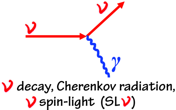
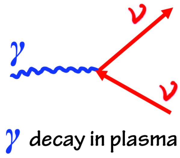
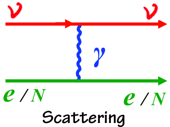
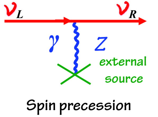
Figure 4: Astrophysical neutrino electromagnetic processes.

The most important neutrino electromagnetic processes are shown in Fig.4 (see, e.g., Refs.16, 19, 14). They are the following: 1) a heavier neutrino decay to a lighter mass state in vacuum, 2) the Cherenkov radiation by a neutrino in matter or an external magnetic field, 3) the spin-light of neutrino in matter, 4) the plasmon decay to a neutrino-antineutrino pair in matter, 5) the neutrino scattering on an electron or a nucleus, and 6) the neutrino spin precession in an external magnetic field and transversely moving (or transversely polarized) matter. All of these processes can be of great interest in astrophysics. The registration of the possible consequences of these processes allows us to obtain information about the values of the electromagnetic properties of neutrinos and also to set appropriate limits. So, astrophysics can be considered as a laboratory for studying the electromagnetic properties of neutrinos (see, e.g., Refs.16, 15, 142).

7.1 Neutrino radiative decay

If neutrinos have nonzero electric charges or transition magnetic or electric moments, a neutrino mass state $\nu_{i}$ can decay into a lighter state $\nu_{f}$ with emission of a photon. This process was discussed for the first time in Ref.[143] and concrete applications to neutrinos can be found in Refs.[144, 145]. For more recent papers and a detailed discussion of neutrino radiative decay $\nu_{i}\rightarrow\nu_{f}+\gamma$, see Refs.[16, 146, 147]. If one neglects the effects of the neutrino charges and charge radii, the neutrino electromagnetic vertex function 15 reduces to

$$\Lambda^{\mu}_{fi}(q)=-i\sigma^{\mu\nu}q_{\nu}\mu_{fi},$$ (57)

where, as before, $\mu_{fi}$ is an effective magnetic moment which includes possible electric moment contributions and we dropped the “eff” superscript for simplicity.

The decay rate in the rest frame of the decaying neutrino $\nu_{i}$ is given by [148, 149]

$$\Gamma_{\nu_{i}\to\nu_{f}+\gamma}=\frac{1}{8\pi}\left(\frac{m_{i}^{2}-m_{f}^{2}}{m_{i}}\right)^{3}|\mu_{fi}|^{2}\simeq 5.4\left(\dfrac{m^{2}_{i}-m^{2}_{f}}{m_{i}^{2}}\right)^{3}\left(\dfrac{m_{i}}{1\,\text{eV}}\right)^{3}\left|\dfrac{\mu_{fi}}{\mu_{\text{B}}}\right|^{2}\text{s}^{-1}.$$ (58)

Note that since $m_{i}\neq m_{f}$ only the transition magnetic and electric moments contribute. Therefore, Eq.58 is equally valid for both Dirac and Majorana neutrinos.

In the simplest extensions of the SM the Dirac and Majorana transition magnetic moments are smaller than $10^{-23}\,\mu_{\text{B}}$ (see Eqs.22 and 23, and Ref.41) and the life time is huge:

$$\tau_{\nu_{i}\rightarrow\nu_{j}+\gamma}\simeq 0.19\times 10^{46}\left(\dfrac{m^{2}_{i}}{m^{2}_{i}-m^{2}_{j}}\right)^{3}\left(\dfrac{1\,\text{eV}}{m_{i}}\right)^{3}\left|\dfrac{10^{-23}\mu_{\text{B}}}{\mu_{fi}}\right|^{2}\text{s}.$$ (59)

The neutrino radiative decay has been constrained from the absence of decay photons in studies of the solar, supernova and reactor (anti)neutrino fluxes, as well as from the absence of the spectral distortions of the cosmic microwave background radiation. However, the corresponding upper bounds on the effective neutrino magnetic moments [15] are in general less stringent than the astrophysical bounds from plasmon decay into a neutrino-antineutrino pair discussed in Section 7.3.

7.2 Neutrino Cherenkov radiation and related processes

Neutrinos with a magnetic moment (and/or an electric charge, as well as an electric moment) propagating in a medium with a velocity larger than the velocity of light in the medium can emit Cherenkov radiation. This possibility was considered for the first time in Ref.[150].

The rate of Cherenkov radiation has been calculated in Ref.[151]. Considering solar neutrinos, the authors of Ref.[151] found that with an effective magnetic moment of $10^{-11}\mu_{\text{B}}$ about five Cherenkov photons in the range of visible light would be emitted per day in a $\text{km}^{3}$ water detector.

In the presence of a magnetic field and/or matter, neutrinos can emit photons by specific mechanisms due to the induced $\nu-\gamma$ effective vertex and the modified photon dispersion relation. In these environments neutrinos can acquire an induced magnetic moment and also an induced electric charge, so that light can be emitted even in the case of massless neutrinos and without the need of BSM effects (see Refs.152, 153, 154, 155, 156, 16).

7.3 Plasmon decay into a neutrino-antineutrino pair

The most interesting astrophysical process for constraining neutrino electromagnetic properties, in particular neutrino magnetic moments, is plasmon decay into a neutrino-antineutrino pair [13]. This process becomes kinematically allowed in media where a photon behaves as a particle with an effective mass $\omega_{\text{P}}$. In a nonrelativistic plasma the dispersion relation for a photon (plasmon) is $\omega_{\gamma}^{2}-{\vec{k}}_{\gamma}^{2}=\omega_{\text{P}}^{2}$, where $\omega_{\text{P}}=\sqrt{4\pi\alpha N_{e}/m_{e}}$ is the plasma frequency ($N_{e}$ is the electron density) [14]. The plasmon decay rate is given by [14]

$$\Gamma_{\gamma^{*}\to\nu{\bar{\nu}}}(\mu_{\nu})=\frac{\mu_{\nu}^{2}}{24\pi}\,Z\,\frac{\omega_{\text{P}}^{4}}{\omega_{\gamma}},$$ (60)

where $Z$ is a factor which depends on the polarization of the plasmon and the effective magnetic moment is given by

$$\mu_{\nu}^{2}=\sum_{k,j}\left(|\mu_{kj}|^{2}+|\epsilon_{kj}|^{2}\right).$$ (61)

A plasmon decay into a neutrino-antineutrino pair transfers the energy $\omega_{\gamma}$ to neutrinos that can freely escape from a star and thus can increase the star cooling speed. The corresponding energy-loss rate per unit volume is

$$Q_{\gamma^{*}\to\nu{\bar{\nu}}}=\frac{g}{(2\pi)^{3}}\int\Gamma_{\gamma^{*}\to\nu{\bar{\nu}}}f_{k_{\gamma}}\omega_{\gamma}d^{3}k_{\gamma},$$ (62)

where $f_{k_{\gamma}}$ is the photon Bose-Einstein distribution function and $g=2$ is the number of polarization states. This energy loss can delay the helium ignition in low-mass red giants and increase the Tip of the Red Giant Branch (TRGB) brightness [14], leading to the TRGB bounds in Table 2. Also the Solar Cooling, Cepheid Stars, and White Dwarfs bounds in Table 2 follow from the energy loss induced by plasmon decay.

The plasmon decay can also be used to constrain the neutrino electric charges [15]. The rate of plasmon decay to a neutrino-antineutrino pair due to the effective neutrino charge $Q_{\nu}=\sqrt{\sum_{k,j}|Q_{kj}|^{2}}$ is given by [14]

$$\Gamma_{\gamma^{*}\to\nu{\bar{\nu}}}(Q_{\nu})=\frac{\alpha Q_{\nu}^{2}}{3}\,Z\,\frac{\omega_{\text{P}}^{2}}{\omega_{\gamma}}.$$ (63)

The corresponding TRGB and solar cooling constraints on $Q_{\nu}$ are listed in Table 4, along with somewhat weaker constraints that are obtained taking into account the Schwinger production of charged $\nu\bar{\nu}$ pairs in the strong electromagnetic field in magnetars.

7.4 Spin light of neutrino

It is known from classical electrodynamics that a system with zero electric charge but nonzero magnetic (or electric) moment can produce electromagnetic radiation which is called “magnetic (or electric) dipole radiation”. It is due to the rotation of the magnetic (or electric) moment. A similar mechanism of radiation exists in the case of a neutrino with a magnetic (or electric) moment propagating in matter [157]. This phenomenon, called “spin light of neutrino” (SL$\nu$), is different from the neutrino Cherenkov radiation in matter discussed in Subsection 7.2, because it can exist even when the emitted photon refractive index is equal to unity. The SL$\nu$ is a radiation produced by the neutrino on its own, rather than a radiation of the background particles. Since the SL$\nu$ process is a transition between neutrino states with equal masses, it can only become possible because of an external environment influence on the neutrino states.

The SL$\nu$ was first studied with a quasi-classical treatment based on a Lorentz-invariant approach to the neutrino spin evolution that implies the use of the generalized Bargmann-Michel-Telegdi equation. The full quantum theory of the SL$\nu$ has been elaborated in Ref.[158]. The quantum theory of the SL$\nu$ method is based on the exact solutions of the modified Dirac equation for the neutrino wave function in matter.

The Feynman diagram of the SL$\nu$ process is shown in Fig.4, where the neutrino initial and final states are exact solutions of the corresponding Dirac equations accounting for the interactions with matter. Here we consider a generic flavor neutrino with an effective magnetic moment $\mu_{\nu}$ and effective mass $m_{\nu}$. The SL$\nu$ process for a relativistic neutrino is a transition from a more energetic neutrino initial state to a less energetic final state with emission of a photon and a neutrino helicity flip.

The amplitude of the SL$\nu$ process is given by

$$S_{fi}=-\mu_{\nu}\sqrt{4\pi}\int d^{4}x{\bar{\psi}}_{f}(x)(\vec{\Gamma}\cdot\vec{\varepsilon}^{*})\frac{e^{ikx}}{\sqrt{2\omega L^{3}}}\psi_{i}(x),\quad\text{where}\quad\vec{\Gamma}=i\omega\big{\{}\big{[}\vec{\Sigma}\times\vec{\varkappa}\big{]}+i\gamma^{5}\vec{\Sigma}\big{\}},\quad\vec{\Sigma}=\begin{pmatrix}\vec{\sigma}&0\\ 0&\vec{\sigma}\end{pmatrix},$$ (64)

and $k^{\mu}=(\omega,{\vec{k}})$ and $\vec{\varepsilon}$ are the photon momentum and polarization vectors, $\vec{\varkappa}=\vec{k}/{\omega}$ is the unit vector pointing in the direction of propagation of the emitted photon. Here $\psi_{i}(x)$ and $\psi_{f}(x)$ are the initial and final neutrino wave functions in presence of matter obtained as exact solutions of the effective Dirac equation. For a relativistic neutrino with momentum $p\gg m_{\nu}$, the total rate $\Gamma$ and power $I$ of SL$\nu$ for different ranges of the effective matter density $\widetilde{N}$ are

$$\Gamma=\left\{\begin{array}[]{lcl}\frac{64}{3}\mu_{\nu}^{2}\widetilde{N}^{3}p^{2}m_{\nu}&\text{for}&\widetilde{N}\ll\frac{m_{\nu}}{p},\\ 4\mu_{\nu}^{2}\widetilde{N}^{2}m_{\nu}^{2}p&\text{for}&\frac{m_{\nu}}{p}\ll\widetilde{N}\ll\frac{p}{m_{\nu}},\\ 4\mu_{\nu}^{2}\widetilde{N}^{3}m_{\nu}^{3}&\text{for}&\widetilde{N}\gg\frac{p}{m_{\nu}},\end{array}\right.\qquad\qquad I=\left\{\begin{array}[]{lcl}\frac{128}{3}\mu_{\nu}^{2}\widetilde{N}^{4}p^{4}&\text{for}&\widetilde{N}\ll\frac{m_{\nu}}{p},\\ \frac{4}{3}\mu_{\nu}^{2}\widetilde{N}^{2}m_{\nu}^{2}p^{2}&\text{for}&\frac{m_{\nu}}{p}\ll\widetilde{N}\ll\frac{p}{m_{\nu}},\\ 4\mu_{\nu}^{2}\widetilde{N}^{4}m_{\nu}^{4}&\text{for}&\widetilde{N}\gg\frac{p}{m_{\nu}}.\end{array}\right.$$ (65)

For a $\nu_{e}$ moving in a medium composed of electrons, protons, and neutrons, the effective matter density is given by

$$\widetilde{N}=\frac{G_{F}}{2{\sqrt{2}}}\Big{[}N_{e}(1+4\sin^{2}\theta_{W})+N_{p}(1-4\sin^{2}\theta_{W})-N_{n}\Big{]},$$ (66)

where $N_{e},N_{p}$, and $N_{n}$ are the number densities of the background electrons, protons, and neutrons, respectively.

Some specific features of this process might have phenomenological consequences in astrophysics (see Ref.159 for a detailed discussion). For a wide range of matter densities, the SL$\nu$ rate and power increase with the neutrino momentum. For ultrahigh-energy neutrinos ($p\sim 10^{18}eV$) propagating through a dense medium with $\widetilde{N}\sim 10\,\text{eV}$ (this value is typical for a neutron star with $N_{n}\sim 10^{38}\,\text{cm}^{-3}$), the rate of the SL$\nu$ process is about $0.7\,\text{s}^{-1}$. This is the most favorable case for the manifestation of the effects of SL$\nu$. It can be realized in galaxy clusters [159]. Moreover, the SL$\nu$ polarization properties may be related to the observed polarization of gamma ray bursts (GRB) [159].

7.5 Neutrino spin and spin-flavor oscillations in magnetic fields and moving matter

The neutrino spin oscillations $\nu_{L}\leftrightarrow\nu_{R}$ induced by the neutrino magnetic moment interaction with a transversal magnetic field $\vec{B}_{\perp}$ were first considered in Ref.[160]. Then spin-flavor oscillations $\nu_{eL}\leftrightarrow\nu_{\mu R}$ in $\vec{B}_{\perp}$ in vacuum were discussed in Ref.[161] and the importance of the matter effect was emphasized in Ref.[162]. The effect of the resonant amplification of neutrino spin oscillations in $\vec{B}_{\perp}$ in the presence of matter was proposed in Refs.[163, 164]. Neutrino spin oscillations in a magnetic field with account for the effect of moving matter was studied in Ref.[165]. A possibility to establish conditions for the resonance in neutrino spin oscillations by the effect of matter motion was discussed in Ref.[166]. The impact of the longitudinal magnetic field $\vec{B}_{||}$ was discussed in Ref.[167]. The effects of non-zero Dirac and Majorana CP violating phases on neutrino-antineutrino oscillations in a magnetic field of astrophysical environments was investigated in Ref.[168]. In particular, it was shown that neutrino-antineutrino oscillations combined with Majorana-type CP violation can affect the $\bar{\nu}_{e}/\nu_{e}$ ratio for neutrinos coming from the supernovae explosion.

The neutrino spin oscillations in the presence of a constant twisting magnetic field were considered in Refs.[169, 170, 171, 172, 173, 174]. In particular, in Ref.[172] the possibility of the transition of up to half of the active left-handed neutrinos into sterile right-handed neutrinos when the neutrino flux leaves the surface of a dense magnetized neutron star (the “cross-border effect”) was predicted.

The resonant spin conversion of neutrinos induced by the geometrical phase in a twisting magnetic field has been studied in Ref.[175]. It has been shown that it could affect the supernova neutronization bursts where very intense magnetic fields are likely. Assuming this mechanism, the measurement of the flavor composition of supernova neutrinos in upcoming neutrino experiments like DUNE and Hyper-Kamiokande can be used as a probe of neutrino magnetic moments, potentially down to a few $10^{-15}\mu_{\text{B}}$ [175].

In Ref.[176] neutrino spin oscillations were considered in the presence of an arbitrary constant electromagnetic field $F_{\mu\nu}$. Neutrino spin oscillations in the presence of the field of circular and linearly polarized electromagnetic waves and superposition of an electromagnetic wave and a constant magnetic field were considered in Refs.[165, 177]. The effect of the parametric resonance in neutrino oscillations in periodically varying electromagnetic fields was studied in Ref.[178].

The more general case of neutrino spin evolution for a neutrino subjected to general types of non-derivative interactions with external scalar $s$, pseudoscalar $\pi$, vector $V_{\mu}$, axial-vector $A_{\mu}$, tensor $T_{\mu\nu}$ and pseudotensor $\Pi_{\mu\nu}$ fields was considered in Ref.[179]. From the general neutrino spin evolution equation, obtained in Ref.[179], it follows that neither scalar $s$, nor pseudoscalar $\pi$, nor vector $V_{\mu}$ fields can induce a neutrino spin evolution. On the contrary, it was shown that electromagnetic (tensor) and weak (axial-vector) interactions can contribute to the neutrino spin evolution.

Neutrino mixing and oscillations in an arbitrary constant magnetic field that have nonzero $\vec{B}_{\perp}$ and $\vec{B}_{||}$ components were considered in Refs.[180, 181, 182].

8 Neutrino magnetic moment portal

Singlet neutral fermions of the Standard Model (SM) gauge group are often introduced to account for the non-zero neutrino mass and are referred to as sterile neutrinos. These sterile neutrinos can interact with the SM sector either through the active-to-sterile mixing portal (see the review in Ref.38) or via the active-to-sterile dipole moment portal. The neutrino dipole portal (NDP) is characterized by the dimension-five operator [183, 184]

$$\mathcal{L}_{\rm NDP}=\bar{N}(i\not{\partial}-m_{N})N+\frac{1}{2}d_{\ell}\bar{N}\sigma_{\mu\nu}\nu_{\ell}F^{\mu\nu}+\text{h.c.},$$ (67)

where $\nu_{\ell}$ is the active neutrino of flavor $\ell$, $N$ is the sterile neutrino with a mass of $m_{N}$, and $d_{\ell}$ is the neutrino transition magnetic moment. In the literature, the unit of $d_{\ell}$ is often chosen as $\text{GeV}^{-1}$, which is inversely proportional to the scale of new physics and can be connected with the traditional unit of $\mu_{\text{B}}$ by the relation

$$d_{\ell}=\frac{\sqrt{\pi\alpha}}{m_{e}}\left|\frac{\mu_{\nu_{\ell}}}{\mu_{\text{B}}}\right|\simeq 296\,{\text{GeV}}^{-1}\left|\frac{\mu_{\nu_{\ell}}}{\mu_{\text{B}}}\right|.$$ (68)

For a broad range of sterile neutrino masses $m_{N}$, the magnetic moment $d_{\ell}$ can be investigated using a variety of methods. In the high mass regime, extending up to 100 GeV, measurements at the electron-positron collider experiments, such as LEP, are capable of probing the magnetic moment at the level of $d_{\ell}\sim 10^{-3}\,\text{GeV}^{-1}$ [184]. In the sub-GeV mass range, sterile neutrinos produced in core-collapse supernovae may escape, carrying away additional energy. This energy loss mechanism imposes constraints, excluding the range $10^{-7}\,\text{GeV}^{-1}\lesssim d_{\ell}\lesssim 10^{-3}\,\text{GeV}^{-1}$ [184]. Below this exclusion band, searches for decay products of sterile neutrinos originating from supernovae, conducted at neutrino detectors [185, 186, 187] and $\gamma-$ray telescopes [185], can potentially probe even smaller values of $d_{\ell}$. To investigate the regions above the supernova cooling band, we can employ high intensity beam dump and neutrino experiments. There are searches via upscattering of atmospheric and solar neutrinos to $N$ which decays at detectors [188, 189], upscattering at Forward LHC detectors [190], Borexino and CHARM-II scattering measurements [142, 191, 192, 193], and the spectrum distortion of neutrino scattering at dark matter detectors [194, 142]. With all these data, $d_{\ell}$ regions above the supernova cooling band for $m_{N}\lesssim 10\,\text{MeV}$ can be probed. For larger $m_{N}$ up to $50\,\text{MeV}$, existing studies can cover the region $d_{\ell}\gtrsim 5\times 10^{-7}\,\text{GeV}^{-1}$, leaving an unexplored region for smaller $d_{\ell}$. The CE$\nu$NS data of reactor neutrinos, neutrinos from the Spallation Neutron Source, and solar neutrinos can address this gap, offering competitive and complementary constraints on sterile neutrino masses up to about 50 MeV.

For the CE$\nu$NS process induced by the NDP when a $\nu_{\ell}$ interacts with a nucleus ${}^{A}_{Z}\mathcal{N}$, the cross section is

$$\dfrac{d\sigma^{\rm NDP}_{\nu_{\ell}}}{dT_{\mathcal{N}}}=d_{\ell}^{2}\alpha Z^{2}[F_{Z}^{\mathcal{N}}(|\hskip-1.0pt\vec{\hskip 1.0ptq}|)]^{2}\left[\frac{1}{T_{\mathcal{N}}}-\frac{1}{E_{\nu}}-\frac{m_{N}^{2}}{2E_{\nu}M_{\mathcal{N}}T_{\mathcal{N}}}\left(1-\frac{M_{\mathcal{N}}-T_{\mathcal{N}}}{2E_{\nu}}\right)-\frac{m_{N}^{4}(M_{\mathcal{N}}-T_{\mathcal{N}})}{8E_{\nu}^{2}M_{\mathcal{N}}^{2}T_{\mathcal{N}}^{2}}\right].$$ (69)

Since the sterile neutrino mass can vary widely, the third term becomes significant when $m_{N}$ is comparable to the energy of the incident neutrino. This offers a unique opportunity to probe the neutrino dipole portal for values of $m_{N}$ in this specific energy range. In the following we are going to show that the CE$\nu$NS interactions of neutrinos from reactors, Spallation Neutron Source, and the Sun can provide unique probes of $d_{e}$, $d_{\mu}$, and $d_{\tau}$.

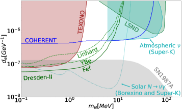
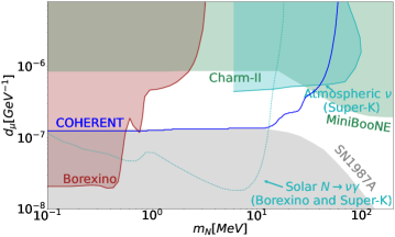
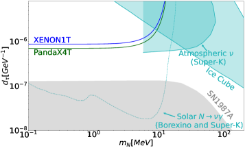
Figure 5: Exclusion limits for the $d_{\ell}$ of a specific flavor at 90$\%$ C.L. From top to bottom, results are shown for $d_{e}$, $d_{\mu}$, $d_{\tau}$. Figure adapted from Ref.[195], see the text for more details.

In Figure 5, which is adapted from Ref.[195], we illustrate the exclusion limits for the $d_{\ell}$ of a specific flavor at 90$\%$ C.L. From top to bottom, the results are shown for $d_{e}$, $d_{\mu}$, $d_{\tau}$. For the CE$\nu$NS COHERENT analysis, the bounds obtained using the energy and time information are shown in blue solid lines. For the Dresden-II reactor antineutrino analysis, the bounds are shown with green solid, dash-dotted and dashed lines using three different quenching models. The limits on $d_{\tau}$ from the solar neutrino CE$\nu$NS experiments XENON1T [196] and PandaX-4T [197] are shown with blue and green solid lines, respectively. Constraints from other experiments are also shown for comparison, including SN1987A [184], TEXONO [115], LSND [184], atmospheric $\nu$ measurement at Super-Kamiokande [189], looking for atmospheric neutrino upscattering to $N$ with subsequent decays, Borexino solar neutrino elastic scattering [142, 198], solar neutrino induced $N\to\nu\gamma$ measurements from Borexino and Super-Kamiokande experiments [188], MiniBooNE [194, 184, 199], Charm-II [194, 200] and IceCube [192]. The results described above concern flavor-specific dipole portals, except for the constraints from SN1987A, where flavor-universal couplings are assumed.

For $d_{e}$, the intense $\bar{\nu}_{e}$ flux of the Dresden-II reactor provides stringent constraints in the low mass range of Figure 5, surpassing the limits from Borexino and Super-Kamiokande, which searched for solar neutrino upscattering to $N$ with subsequent decays [189], as well as those from TEXONO [115], which measured reactor $\bar{\nu}_{e}$ E$\nu$ES. The constraints from COHERENT, based on a fit that includes both the energy and timing information, extend to $m_{N}\sim 50\,\text{MeV}$. The COHERENT bound is as competitive as those from LSND [184] and atmospheric $\nu$ measurements at Super-Kamiokande, which are based on the non-observation of atmospheric neutrino upscattering to $N$ with subsequent decays [189]. It is important to note that different choices of quenching models in the analysis of the Dresden-II CE$\nu$NS data can significantly affect the constraints in the low mass region.

The COHERENT CE$\nu$NS data provide the most stringent constraints on $d_{\mu}$ in the energy range at tens of MeV, with limits reaching as low as about $1\times 10^{-7}\,\text{GeV}^{-1}$ below 10 MeV. By using both the energy and time information of the COHERENT CE$\nu$NS data, the effects induced by the $\nu_{\mu}$ flux can be distinguished from those induced by the $\bar{\nu}_{\mu}$ and $\bar{\nu}_{e}$ fluxes and different limits are obtained for $d_{e}$ and $d_{\mu}$. For comparison, the constraints from other experiments such as MiniBooNE [194, 184, 199], CHARM-II [194, 200], solar neutrino E$\nu$ES observations at Borexino [142, 198], and atmospheric $\nu$ measurements at Super-K [189] are also illustrated in Figure 5.

Since a substantial portion of the solar neutrino flux detected on Earth is made of $\nu_{\tau}$, the CE$\nu$NS measurements of solar neutrinos in dark matter direct detection experiments offer an opportunity to probe the value of $d_{\tau}$. The limits on $d_{\tau}$ from XENON1T [196] and PandaX-4T [197] in Figure 5 have been obtained from the 90% C.L. upper limits on the ⁸B solar neutrino flux established by these two experiments with CE$\nu$NS data. The XENON1T and PandaX-4T upper limits on $d_{\tau}$ are below $10^{-6}\,\text{GeV}^{-1}$ for $m_{N}\lesssim 10\,\text{MeV}$ and agree with the more stringent Borexino and Super-Kamiokande limit. Taking into account the recent measurements of CE$\nu$NS produced by ⁸B solar neutrinos by the PandaX-4T [201] and XENONnT [202] experiments, we expect substantial improvements in the search of neutrino magnetic moments with solar CE$\nu$NS experiments in the future.

9 Conclusions and future prospects

The search of neutrino electromagnetic interactions is an important tool for testing the Standard Model (SM) and for discovering new physics Beyond the Standard Model (BSM). The SM can be tested by measuring the charge radii of the three flavor neutrinos predicted by the calculation of the SM radiative corrections. The observation of different values of the neutrino charge radii or other neutrino electromagnetic interactions would be a discovery of BSM physics.

The current limits in Table 3 on the values of the flavor neutrinos charge radii are only about one order of magnitude larger than the SM predictions in Eq.43. Therefore, the neutrino charge radii may be the first neutrino electromagnetic property that will be discovered in future experiments with higher precision. However, most experimental and theoretical studies are devoted to neutrino magnetic moments, which are predicted by many BSM models and are connected with the neutrino masses. The current upper bounds on the neutrino magnetic moments in Tables 1 and 2, obtained from the data of laboratory experiments and analyses of astrophysical data, are more than seven orders of magnitude larger than the predictions of the simplest extensions of the SM (see Eqs.20–23). However, the search of the effects of the neutrino magnetic moments below the current limits is motivated by the predictions of larger values of the neutrino magnetic moments by more elaborate BSM models with Dirac [203] or Majorana [40, 44, 45, 46, 47, 48] neutrinos. The neutrino charges, sometimes called “millicharges”, are usually considered more exotic, but they are worth searching for, since they are associated with a possible charge dequantization [138, 139, 16, 18].

The current best limit on a neutrino magnetic moment obtained in a laboratory experiment is the bound on $\mu_{\nu_{e}}$ obtained by the GEMMA [53] experiment (see Table 1). Most of the astrophysical limits on the neutrino magnetic moments in Table 2 are more stringent, but they suffer from astrophysical uncertainties. Therefore, it is important to continue the search of the effects of the neutrino electromagnetic properties in laboratory experiments where the neutrino beam is under control. Note that novel detection methods such as the enhancement of the screening effect in semiconductor detectors [204] could push the limit on the neutrino magnetic moment down to $10^{-13}\,\mu_{\text{B}}$.

Future improvements in the search of neutrino electromagnetic interactions are expected from the results of the GEMMA II [205], TEXONO [206], JUNO-TAO [207, 208], CLOUD [208], SHIP [209], FPF@LHC [210], SBN [211], ESS [212], DUNE [213] experiments, CE$\nu$NS experiments [214, 20], CE$\nu$AS experiments [215], in particular the SATURNE project [216], experiments with a radioactive [217] or an IsoDAR [218] source near an appropriate detector, as well as from analyses of improved astrophysical data, especially the dark matter and solar neutrino experiments PandaX [201], XENONnT [202, 219], LUX-ZEPLIN [220, 72], XMASS [70], DARWIN [124, 79], XLZD [125], DarkSide [126].

In conclusion, we expect an interesting future for the search of neutrino electromagnetic properties.

DISCLOSURE STATEMENT

The authors are not aware of any affiliations, memberships, funding, or financial holdings that might be perceived as affecting the objectivity of this review.

References

- [1] Navas S, et al. Phys. Rev. D 110(3):030001 (2024)
- [2] Giunti C, Kim CW. Oxford, UK: Fundamentals of Neutrino Physics and Astrophysics, Oxford University Press (2007)
- [3] Bilenky S. Introduction to the Physics of Massive and Mixed Neutrinos, Springer (2018)
- [4] Coloma P, Koerner LW, Shoemaker IM, Yu J. arXiv:2209.10362 (2022)
- [5] Pauli W. Phys. Today 31N9:27 (1978)
- [6] Carlson JF, Oppenheimer JR. Phys. Rev. 41:763–792 (1932)
- [7] Bethe H. Proc. Cambridge Philos. Soc. 31:108 (1935)
- [8] Cowan CL, Reines F, Harrison FB, Kruse HW, McGuire AD. Science 124:103–104 (1956)
- [9] Bethe H, Peierls R. Nature 133:532 (1934)
- [10] Nahmias ME. Math. Proc. Cambridge Phil. Soc. 31(01):99 (1935)
- [11] Cowan CL, Reines F, Harrison FB. Phys. Rev. 96:1294 (1954)
- [12] Cowan CL, Reines F. Phys. Rev. 107:528–530 (1957)
- [13] Bernstein J, Ruderman M, Feinberg G. Phys. Rev. 132:1227–1233 (1963)
- [14] Raffelt GG. Stars as laboratories for fundamental physics, University of Chicago Press (1996)
- [15] Raffelt GG. Ann. Rev. Nucl. Part. Sci. 49:163–216 (1999)
- [16] Giunti C, Studenikin A. Rev.Mod.Phys. 87:531 (2015)
- [17] Baha Balantekin A, Kayser B. Ann. Rev. Nucl. Part. Sci. 68:313–338 (2018)
- [18] Das A, Ghosh D, Giunti C, Thalapillil A. Phys. Rev. D 102(11):115009 (2020)
- [19] Studenikin A. PoS CORFU2021:057 (2022)
- [20] Abdullah M, et al. arXiv:2203.07361 (2022)
- [21] Fukuda Y, et al. Phys. Rev. Lett. 81:1562–1567 (1998)
- [22] de Salas PF, Forero DV, Gariazzo S, Martinez-Mirave P, Mena O, et al. JHEP 2021:071 (2020)
- [23] Esteban I, Gonzalez-Garcia MC, Maltoni M, Schwetz T, Zhou A. JHEP 09:178 (2020)
- [24] Capozzi F, Di Valentino E, Lisi E, Marrone A, Melchiorri A, Palazzo A. Phys.Rev.D 104:083031 (2021)
- [25] Abusleme A, et al. Prog.Part.Nucl.Phys. 123:103927 (2022)
- [26] Abi B, et al. Eur.Phys.J. C80:978 (2020)
- [27] Bian J, et al. arXiv:2203.02029 (2022)
- [28] Alekou A, et al. Eur. Phys. J. C 81(12):1130 (2021)
- [29] Bernabeu J, Cabral-Rosetti LG, Papavassiliou J, Vidal J. Phys. Rev. D62:113012 (2000)
- [30] Bernabeu J, Papavassiliou J, Vidal J. Phys. Rev. Lett. 89:101802 (2002)
- [31] Bernabeu J, Papavassiliou J, Vidal J. Nucl. Phys. B680:450 (2004)
- [32] Erler J, Su S. Prog. Part. Nucl. Phys. 71:119–149 (2013)
- [33] Gariazzo S, Giunti C, Laveder M, Li YF, Zavanin EM. J. Phys. G43:033001 (2016)
- [34] Adhikari R, et al. JCAP 1701:025 (2017)
- [35] Boyarsky A, Drewes M, Lasserre T, Mertens S, Ruchayskiy O. Prog.Part.Nucl.Phys. 104:1–45 (2019)
- [36] Giunti C, Lasserre T. Ann. Rev. Nucl. Part. Sci. 69:163–190 (2019)
- [37] Boser S, Buck C, Giunti C, Lesgourgues J, Ludhova L, et al. Prog.Part.Nucl.Phys. 111:103736 (2020)
- [38] Dasgupta B, Kopp J. Phys.Rept. 928:63 (2021)
- [39] Fujikawa K, Shrock R. Phys. Rev. Lett. 45:963 (1980)
- [40] Pal PB, Wolfenstein L. Phys. Rev. D25:766 (1982)
- [41] Shrock RE. Nucl. Phys. B206:359 (1982)
- [42] Dvornikov M, Studenikin A. Phys. Rev. D69:073001 (2004)
- [43] Dvornikov M, Studenikin A. J. Exp. Theor. Phys. 99:254 (2004)
- [44] Barr SM, Freire EM, Zee A. Phys. Rev. Lett. 65:2626–2629 (1990)
- [45] Babu KS, Mohapatra RN. Phys. Rev. D42:3778–3793 (1990)
- [46] Pal BK. Phys. Rev. D44:2261–2264 (1991)
- [47] Boyarkin OM, Boyarkina GG. Phys. Rev. D 90(2):025001 (2014)
- [48] Lindner M, Radovcic B, Welter J. JHEP 1707:139 (2017)
- [49] Vidyakin GS, Vyrodov VN, Gurevich II, Kozlov YV, Martemyanov VP, et al. JETP Lett. 55:206–210 (1992)
- [50] Derbin AI, et al. JETP Lett. 57:768–772 (1993)
- [51] Daraktchieva Z, et al. Phys. Lett. B615:153 (2005)
- [52] Wong HT, et al. Phys. Rev. D75:012001 (2007)
- [53] Beda AG, Brudanin VB, Egorov VG, Medvedev DV, Pogosov VS, et al. Adv.High Energy Phys. 2012:350150 (2012)
- [54] Bonet H, et al. Eur.Phys.J.C 82:813 (2022)
- [55] Allen RC, Chen HH, Doe PJ, Hausammann R, Lee WP, et al. Phys. Rev. D47:11–28 (1993)
- [56] Ahrens LA, Aronson SH, Connolly PL, Gibbard BG, Murtagh MJ, et al. Phys. Rev. D41:3297–3316 (1990)
- [57] Auerbach LB, et al. Phys. Rev. D63:112001 (2001)
- [58] Grassler H, et al. Nucl. Phys. B273:253 (1986)
- [59] Cooper-Sarkar AM, Sarkar S, Guy J, Venus W, Hulth PO, Hultqvist K. Phys. Lett. B 280:153–158 (1992)
- [60] Schwienhorst R, et al. Phys. Lett. B513:23–29 (2001)
- [61] Akimov D, et al. Phys.Rev.Lett. 126:012002 (2021)
- [62] Akimov D, et al. Phys. Rev. Lett. 129(8):081801 (2022)
- [63] Coloma P, Esteban I, Gonzalez-Garcia MC, Larizgoitia L, Monrabal F, Palomares-Ruiz S. JHEP 05:037 (2022)
- [64] Atzori Corona M, Cadeddu M, Cargioli N, Dordei F, Giunti C, et al. JHEP 09:164 (2022)
- [65] Colaresi J, Collar JI, Hossbach TW, Lewis CM, Yocum KM. Phys. Rev. Lett. 129(21):211802 (2022)
- [66] Grotch H, Robinett RW. Z. Phys. C 39:553 (1988)
- [67] Tanimoto N, Nakano I, Sakuda M. Phys. Lett. B 478:1–4 (2000)
- [68] Liu DW, et al. Phys. Rev. Lett. 93:021802 (2004)
- [69] Agostini M, et al. Phys.Rev. D96:091103 (2017)
- [70] Abe K, et al. Phys.Lett. B:135741 (2020)
- [71] Aprile E, et al. Phys. Rev. Lett. 129(16):161805 (2022)
- [72] Aalbers J, et al. Phys. Rev. D 108(7):072006 (2023)
- [73] Zeng X, et al. arXiv:2408.07641 (2024)
- [74] Aalbers J, et al. Phys. Rev. Lett. 131(4):041002 (2023)
- [75] Atzori Corona M, Bonivento WM, Cadeddu M, Cargioli N, Dordei F. Phys.Rev.D 107:053001 (2023)
- [76] Khan AN. Phys.Lett.B 837:137650 (2023)
- [77] ShivaSankar KA, Majumdar A, Papoulias DK, Prajapati H, Srivastava R. Phys.Lett.B 839:137742 (2023)
- [78] Zhang D, et al. Phys. Rev. Lett. 129(16):161804 (2022)
- [79] Giunti C, Ternes CA. Phys. Rev. D 108(9):095044 (2023)
- [80] Barbieri R, Mohapatra RN. Phys. Rev. Lett. 61:27 (1988)
- [81] Ayala A, D’Olivo JC, Torres M. Phys. Rev. D59:111901 (1999)
- [82] Ayala A, D’Olivo JC, Torres M. Nucl. Phys. B564:204–222 (2000)
- [83] Kuznetsov AV, Mikheev NV, Okrugin AA. Int. J. Mod. Phys. A 24:5977–5989 (2009)
- [84] Raffelt GG. Phys. Rev. Lett. 64:2856–2858 (1990)
- [85] Castellani V, Degl’Innocenti S. Astrophys.J. 402:574–578 (1993)
- [86] Viaux N, Catelan M, Stetson PB, Raffelt G, Redondo J, et al. Astron. Astrophys. 558:A12 (2013)
- [87] Arceo-Díaz S, Schröder KP, Zuber K, Jack D. Astropart. Phys. 70:1–11 (2015)
- [88] Capozzi F, Raffelt G. Phys. Rev. D 102(8):083007 (2020)
- [89] Mori K, Kusakabe M, Balantekin AB, Kajino T, Famiano MA. Mon.Not.Roy.Astron.Soc. 503:2746–2753 (2021)
- [90] Franz N, Dennis M, Sakstein J. arXiv:2307.13050 (2023)
- [91] Raffelt GG. Phys. Rept. 320:319–327 (1999)
- [92] Mori K, Balantekin AB, Kajino T, Famiano MA. Astrophys.J. 901:115 (2020)
- [93] Corsico AH, Althaus LG, Miller Bertolami MM, Kepler SO, Garcia-Berro E. JCAP 08:054 (2014)
- [94] Miller Bertolami MM. Astron. Astrophys. 562:A123 (2014)
- [95] Morgan JA. Phys. Lett. B102:247–250 (1981)
- [96] Elmfors P, Enqvist K, Raffelt G, Sigl G. Nucl. Phys. B503:3–23 (1997)
- [97] Grohs E, Balantekin AB. Phys.Rev.D 107:123502 (2023)
- [98] Li SP, Xu XJ. JHEP 02:085 (2023)
- [99] Carenza P, Lucente G, Gerbino M, Giannotti M, Lattanzi M. Phys. Rev. D 110(2):023510 (2024)
- [100] Akimov D, et al. Science 357(6356):1123–1126 (2017)
- [101] Fayans SA, Mikaelyan LA, Sinev VV. Phys. Atom. Nucl. 64:1475–1480 (2001)
- [102] Kouzakov KA, Studenikin AI. Adv. High Energy Phys. 2014:569409 (2014)
- [103] Chen JW, et al. Phys.Lett. B731:159–162 (2014)
- [104] Cadeddu M, Dordei F, Giunti C. EPL 143(3):34001 (2023)
- [105] Freedman DZ. Phys. Rev. D 9:1389–1392 (1974)
- [106] Xu J, Barbeau PS, Hong Z. Ann. Rev. Nucl. Part. Sci. 73(1):95–121 (2023)
- [107] Barranco J, Miranda OG, Rashba TI. JHEP 12:021 (2005)
- [108] Atzori Corona M, Cadeddu M, Cargioli N, Dordei F, Giunti C, Masia G. Eur. Phys. J. C 83(7):683 (2023)
- [109] Grimus W, Stockinger P. Phys. Rev. D57:1762–1768 (1998)
- [110] Beacom JF, Vogel P. Phys. Rev. Lett. 83:5222–5225 (1999)
- [111] Kopp J, Opferkuch T, Wang E. JCAP 03:043 (2024)
- [112] Brdar V, Cheng T, Kuan HJ, Li YY. JCAP 07:026 (2024)
- [113] Cadeddu M, Giunti C, Kouzakov KA, Li YF, Zhang YY, Studenikin AI. Phys. Rev. D 98(11):113010 (2018), [Erratum: Phys.Rev.D 101, 059902 (2020)]
- [114] Kouzakov KA, Studenikin AI. Phys. Rev. D 95(5):055013 (2017), [Erratum: Phys.Rev.D 96, 099904 (2017)]
- [115] Deniz M, et al. Phys. Rev. D81:072001 (2010)
- [116] Zeller GP, et al. Phys. Rev. Lett. 88:091802 (2002), [Erratum: Phys.Rev.Lett. 90, 239902 (2003)]
- [117] Hirsch M, Nardi E, Restrepo D. Phys. Rev. D67:033005 (2003)
- [118] Vilain P, et al. Phys. Lett. B345:115–118 (1995)
- [119] McFarland KS, et al. Eur. Phys. J. C1:509–513 (1998)
- [120] Grifols JA, Masso E. Mod. Phys. Lett. A 2:205 (1987)
- [121] Grifols JA, Masso E. Phys. Rev. D 40:3819 (1989)
- [122] Altherr T, Salati P. Nucl. Phys. B 421:662–682 (1994)
- [123] Atzori Corona M, Cadeddu M, Cargioli N, Dordei F, Giunti C. JHEP 05:271 (2024)
- [124] Aalbers J, et al. Eur. Phys. J. C 80(12):1133 (2020)
- [125] Aalbers J, et al. arXiv:2410.17137 (2024)
- [126] Acerbi F, et al. arXiv:2407.05813 (2024)
- [127] Hughes V, Fraser L, Carlson E. Z. Phys. D 10:145 (1988)
- [128] Bressi G, Carugno G, valle FD, Galeazzi G, Ruoso G, et al. Phys. Rev. A83(5):052101 (2011)
- [129] Della Valle F, Ejlli A, Gastaldi U, Messineo G, Milotti E, et al. Eur. Phys. J. C 76(1):24 (2016)
- [130] Li HB. Phys. Rev. Lett. 90:131802 (2003)
- [131] Gninenko SN, Krasnikov NV, Rubbia A. Phys. Rev. D75:075014 (2007)
- [132] Studenikin A. Europhys.Lett. 107:21001 (2014)
- [133] Chen JW, Chi HC, Li HB, Liu CP, Singh L, et al. Phys. Rev. D90(1):011301 (2014)
- [134] Babu KS, Gould TM, Rothstein IZ. Phys.Lett. B321:140–144 (1994)
- [135] Studenikin AI, Tokarev I. Nucl. Phys. B 884:396–407 (2014)
- [136] Barbiellini G, Cocconi G. Nature 329:21–22 (1987)
- [137] Fung A, Heeba S, Liu Q, Muralidharan V, Schutz K, Vincent AC. Phys. Rev. D 109(8):083011 (2024)
- [138] Foot R, Joshi GC, Lew H, Volkas RR. Mod.Phys.Lett. A5:2721–2732 (1990)
- [139] Foot R, Lew H, Volkas RR. J. Phys. G19:361–372 (1993)
- [140] Karshenboim SG. arXiv:2406.19129 (2024)
- [141] Caprini C, Ferreira PG. JCAP 02:006 (2005)
- [142] Brdar V, Greljo A, Kopp J, Opferkuch T. JCAP 01:039 (2021)
- [143] Shrock R. Phys. Rev. D 9:743–748 (1974)
- [144] Petcov ST. Sov. J. Nucl. Phys. 25:340 (1977), [Erratum: Sov.J.Nucl.Phys. 25, 698 (1977)]
- [145] Zatsepin G, Smirnov AY. Yad.Fiz. 28:1569–1579 (1978)
- [146] Balaji S, Ramirez-Quezada M, Zhou YL. JHEP 04:178 (2020)
- [147] Balaji S, Ramirez-Quezada M, Zhou YL. JHEP 12:090 (2020)
- [148] Marciano WJ, Sanda AI. Phys. Lett. B 67:303–305 (1977)
- [149] Lee BW, Shrock RE. Phys. Rev. D 16:1444 (1977)
- [150] Radomski M. Phys. Rev. D 12:2208–2211 (1975)
- [151] Grimus W, Neufeld H. Phys. Lett. B 315:129–133 (1993)
- [152] Galtsov DV, Nikitina NS. Zh. Eksp. Teor. Fiz. 62:2008–2012 (1972)
- [153] Giunti C, Kim CW, Lee UW, Lam WP. Phys. Rev. D 45:1557–1568 (1992)
- [154] Oraevsky VN, Semikoz VB, Smorodinsky YA. JETP Lett. 43:709–712 (1986)
- [155] Ioannisian AN, Raffelt GG. Phys. Rev. D 55:7038–7043 (1997)
- [156] Ternov AI. Phys. Rev. D 94(9):093008 (2016)
- [157] Lobanov A, Studenikin A. Phys. Lett. B 564(1):27–34 (2003)
- [158] Studenikin A, Ternov A. Phys. Lett. B 608:107–114 (2005)
- [159] Grigoriev A, Lokhov A, Studenikin A, Ternov A. JCAP 11:024 (2017)
- [160] Cisneros A. Astrophys. Space Sci. 10:87–92 (1971)
- [161] Schechter J, Valle JWF. Phys. Rev. D 24:1883–1889 (1981), [Erratum: Phys.Rev.D 25, 283 (1982)]
- [162] Okun LB, Voloshin MB, Vysotsky MI. Sov. J. Nucl. Phys. 44:440 (1986)
- [163] Akhmedov EK. Phys. Lett. B 213:64–68 (1988)
- [164] Lim CS, Marciano WJ. Phys. Rev. D 37:1368–1373 (1988)
- [165] Lobanov AE, Studenikin AI. Phys. Lett. B 515:94–98 (2001)
- [166] Studenikin AI. Phys. Atom. Nucl. 67:993–1002 (2004)
- [167] Akhmedov EK, Khlopov MY. Mod. Phys. Lett. A 3:451–457 (1988)
- [168] Popov A, Studenikin A. Phys. Rev. D 103:115027 (2021)
- [169] Vidal J, Wudka J. Phys. Lett. B 249:473–477 (1990)
- [170] Smirnov AY. Phys. Lett. B 260:161–164 (1991)
- [171] Akhmedov EK, Petcov ST, Smirnov AY. Phys. Rev. D 48:2167–2181 (1993)
- [172] Likhachev GG, Studenikin AI. J. Exp. Theor. Phys. 81:419–425 (1995)
- [173] Dvornikov M. J. Phys. G 35:025003 (2008)
- [174] Dmitriev A, Fabbricatore R, Studenikin A. PoS CORFU2014:050 (2015)
- [175] Jana S, Porto Y. Phys. Rev. Lett. 132(10):101005 (2024)
- [176] Egorov AM, Lobanov AE, Studenikin AI. Phys. Lett. B 491:137–142 (2000)
- [177] Dvornikov MS, Studenikin AI. Phys. Atom. Nucl. 64:1624–1627 (2001)
- [178] Dvornikov MS, Studenikin AI. Phys. Atom. Nucl. 67:719–725 (2004)
- [179] Dvornikov M, Studenikin A. JHEP 09:016 (2002)
- [180] Fabbricatore R, Grigoriev A, Studenikin A. J. Phys. Conf. Ser. 718(6):062058 (2016)
- [181] Studenikin A. EPJ Web Conf. 125:04018 (2016)
- [182] Kurashvili P, Kouzakov KA, Chotorlishvili L, Studenikin AI. Phys. Rev. D 96(10):103017 (2017)
- [183] Schwetz T, Zhou A, Zhu JY. JHEP 21:200 (2020)
- [184] Magill G, Plestid R, Pospelov M, Tsai YD. Phys. Rev. D 98(11):115015 (2018)
- [185] Brdar V, de Gouvêa A, Li YY, Machado PAN. Phys. Rev. D 107(7):073005 (2023)
- [186] Chauhan G, Horiuchi S, Huber P, Shoemaker IM. Phys. Rev. D 110(1):015007 (2024)
- [187] Lazar J, Li YY, Arguelles CA, Brdar V. arXiv:2403.09781 (2024)
- [188] Plestid R. Phys. Rev. D 104:075027 (2021)
- [189] Gustafson RA, Plestid R, Shoemaker IM. Phys. Rev. D 106(9):095037 (2022)
- [190] Ismail A, Jana S, Abraham RM. Phys. Rev. D 105(5):055008 (2022)
- [191] Agostini M, et al. Nature 562(7728):505–510 (2018)
- [192] Coloma P, Machado PAN, Martinez-Soler I, Shoemaker IM. Phys. Rev. Lett. 119(20):201804 (2017)
- [193] Geiregat D, et al. Phys. Lett. B 259:499–507 (1991)
- [194] Shoemaker IM, Wyenberg J. Phys. Rev. D 99(7):075010 (2019)
- [195] Li YY, Li YF, Xia SY. arXiv:2406.07477 (2024)
- [196] Aprile E, et al. Phys. Rev. Lett. 126:091301 (2021)
- [197] Ma W, et al. Phys. Rev. Lett. 130(2):021802 (2023)
- [198] Redchuk M. PoS EPS-HEP2019:400 (2020)
- [199] Aguilar-Arevalo AA, et al. Phys. Rev. Lett. 98:231801 (2007)
- [200] Geiregat D, et al. Phys. Lett. B 232:539 (1989)
- [201] Bo Z, et al. arXiv:2407.10892 (2024)
- [202] Aprile E, et al. arXiv:2408.02877 (2024)
- [203] Bolanos-Carrera A, Guiot-Lomeli M, Tavares-Velasco G. Eur. Phys. J. C 84(3):217 (2024)
- [204] Li YF, Xia Sy. JHEP 10:021 (2023)
- [205] Alekseev I, et al. J. Phys. Conf. Ser. 934(1):012006 (2017)
- [206] Singh MK, Sharma V, Singh L, Chen JH, Singh V, et al. Indian J. Phys. 91(10):1277–1291 (2017)
- [207] Abusleme A, et al. arXiv:2005.08745 (2020)
- [208] Brdar V, Ferreira Leite LJ, Parker GA, Xu XJ. arXiv:2410.00107 (2024)
- [209] Ahdida C, et al. Eur. Phys. J. C 82(5):486 (2022)
- [210] Mammen Abraham R, Foroughi-Abari S, Kling F, Tsai YD. arXiv:2301.10254 (2023)
- [211] Machado PA, Palamara O, Schmitz DW. Ann. Rev. Nucl. Part. Sci. 69:363–387 (2019)
- [212] Baxter D, et al. JHEP 02:123 (2020)
- [213] Mathur V, Shoemaker IM, Tabrizi Z. JHEP 10:041 (2022)
- [214] Barbeau PS, Efremenko Y, Scholberg K. Ann. Rev. Nucl. Part. Sci. 73:41–68 (2023)
- [215] Cadeddu M, Dordei F, Giunti C, Kouzakov KA, Picciau E, Studenikin AI. Phys. Rev. D 100(7):073014 (2019)
- [216] Cadeddu M, et al. Mosc. Univ. Phys. Bull. 79(Suppl. 1):S240–S248 (2024)
- [217] Herrera G, Huber P. arXiv:2408.11904 (2024)
- [218] Winklehner D, et al. arXiv:2404.06281 (2024)
- [219] Herrera G. JHEP 05:288 (2024)
- [220] Akerib DS, et al. Phys. Rev. D 104(9):092009 (2021)