Testing Generalizability in Causal Inference
Daniel de Vassimon Manela1,* Linying Yang1,* Robin J. Evans1 1Department of Statistics, University of Oxford *Equal Contribution
Abstract
Ensuring robust model performance across diverse real-world scenarios requires addressing both transportability across domains with covariate shifts and extrapolation beyond observed data ranges. However, there is no formal procedure for statistically evaluating generalizability in machine learning algorithms, particularly in causal inference. Existing methods often rely on arbitrary metrics like AUC or MSE and focus predominantly on toy datasets, providing limited insights into real-world applicability. To address this gap, we propose a systematic and quantitative framework for evaluating model generalizability under covariate distribution shifts, specifically within causal inference settings. Our approach leverages the frugal parameterization, allowing for flexible simulations from fully and semi-synthetic benchmarks, offering comprehensive evaluations for both mean and distributional regression methods. By basing simulations on real data, our method ensures more realistic evaluations, which is often missing in current work relying on simplified datasets. Furthermore, using simulations and statistical testing, our framework is robust and avoids over-reliance on conventional metrics. Grounded in real-world data, it provides realistic insights into model performance, bridging the gap between synthetic evaluations and practical applications.
1 INTRODUCTION
Algorithm generalizability has garnered significant interest in fields such as computer vision and natural language processing. It encompasses both transportability under covariate shifts between domains and extrapolation, where predictions are made within the same population but beyond the observed data range or in underrepresented subgroups.
Generalizability has also become a central focus in causal inference (Bareinboim and Pearl,, 2016; Curth et al.,, 2021; Johansson et al.,, 2018; Buchanan et al.,, 2018; Ling et al.,, 2022; Bica and Schaar,, 2022). Here, it refers to the ability of a causal model to make accurate causal predictions or draw valid causal conclusions when applied to data from a domain or distribution other than the one it was trained on. This concept is crucial when the objective involves understanding and predicting the effects of interventions across various settings. These settings may significantly diverge from the original conditions under which the model was developed, presenting challenges due to variations in factors such as environment, demographics, or other external influences. This holds particular importance in clinical settings, where the growing interest in personalized treatment and patient stratification underscores the need for generalize inferences across diverse population domains.
Although strategies for improving generalization have been widely explored (Zhou et al.,, 2022; Yu et al.,, 2024), there has been comparatively little focus on developing a comprehensive, structured framework for evaluating generalizability. A common approach is to measure generalization or extrapolation performance using metrics like AUC for classification or MSE for regression. However, these metrics often lack informativeness. Achieving an MSE of 5, compared to 10 from other methods, on synthetic data irrelevant to the user’s intended application, does not provide clear guarantees regarding real-world performance. Therefore, it is essential to establish a systematic evaluation framework based on simulation for generalizability performance, which can offer a more robust and comprehensive understanding of how these methods perform on relevant tasks.
This paper proposes a method to statistically evaluate the generalizability of causal inference algorithms under covariate and treatment distribution shifts. We introduce a semi-synthetic simulation framework using two domains – training (A) and testing (B) – that share the same intervened conditional outcome distributions but potentially differ in covariate and treatment distributions. A model is trained on domain A to learn the shared high dimensional conditional outcome distribution. We test the model’s generalizability by estimating the marginal causal quantities in domain B, where these values are explicitly known. This approach simplifies the evaluation process by reducing the complexity from higher-dimensional intervened models to a lower-dimensional causal effect, enabling more powerful statistical testing.
A high-level overview of the workflow of our method:
-
1.
Learn both the distribution parameters of two domains, and the Conditional Outcome Distribution (COD) from real-world data: Define two domains, domain A and domain B, of which the covariate and treatment distributions can be different, but the COD is the same. These distributions can be learned empirically from real-world data, rather than just being limited to specifying parametric models.
-
2.
Model training: Simulate semi-synthetic data from domain A using the distributions fitted on data. Train a conditional effect model on the simulated data.
-
3.
Prediction/Estimaton: Simulate data from domain B, whose covariate and treatment distributions may differ from domain A, but with an identical COD. Apply the trained model on the sampled covariates and treatments from domain B and estimate marginal causal quantities outcome predictions from the model.
-
4.
Evaluate generalizability with statistical testing: Statistically test whether the estimated marginal causal quantities deviate significantly from the known ground truth in domain B. This provides an evaluation of the model’s generalizability under covariate and treatment distribution shifts. The tests assess whether the model generalizes effectively by focusing on lower-dimensional quantities instead of high-dimensional conditional outcome models.
Main Contributions
In this work, we propose a formal framework for statistically testing the generalizability of machine learning algorithms under covariate and treatment distribution shifts, specifically in the context of causal inference. Rather than relying on arbitrary metric scores, we provide tests that statistically evaluate the ability of both mean and distributional regression methods regarding generalizability. This provides a simple and effective solution for assessing how well algorithms account for these complexities in real-world applications.
Consequently, we claim that our evaluation method is:
-
•
Systematic: We offer a structured framework that allows users to easily specify and input flexible data generation processes for simulations.
-
•
Comprehensive: Our method supports simulations from various data generation processes, covering both continuous and discrete covariates and outcomes.
-
•
Robust: We incorporate statistical testing to evaluate the generalizability of distributional and mean regression models.
-
•
Realistic: Simulations can be based on actual data, bridging the gap between synthetic evaluations and real-world applications.
2 BACKGROUND
Throughout the paper, we consider a static treatment model with an outcome and a general treatment which can be either continuous or discrete. Let the set of measured pretreatment covariates be . If we make the standard assumptions of SUTVA, positivity, and conditional ignorability outlined in Pearl, (2009), we define the marginal causal treatment density as follows:
| (1) |
which is the marginalized over the randomized model.
We also use to denote the marginal potential outcome given the intervention. Correspondingly, we use to denote the conditional expectation of that potential outcome given covariate values. Note that can be read as in some notations. When the treatment is binary, we define as the average treatment effect (ATE), quantifying the overall impact of a treatment or intervention across the entire population. Similarly, let be the conditional average treatment effect (CATE), measuring the expected impact of an intervention for specific subgroups or individuals, capturing treatment effect heterogeneity.
We aim to evaluate the generalizability of an outcome regression model that predicts the expected outcome , with the model’s predicted outcomes indicated by a hat symbol.
2.1 Generalizability in Causal Inference
Extensive research has focused on generalizability in causal inference, as mentioned in the Introduction. As highlighted by Ling et al., (2022), three common approaches are used to assess treatment effect generalizability: inverse probability of sampling weighting (IPSW) methods that adjust for differences between study and target populations by weighting based on sample inclusion probabilities (Buchanan et al.,, 2018); outcome model-based methods that estimate the conditional outcome directly (Kern et al.,, 2016); and the hybrid approaches that combines both (Dahabreh et al.,, 2019).
In this work, we focus on algorithms that generalize outcome predictions across different domains, enabling accurate CATE or COD estimation. This is crucial for understanding individual-level treatment effect heterogeneity and ensuring models can adapt to new populations or environments with varying covariate distributions. A summary of common CATE estimation methods is provided by Caron et al., (2022).
Despite advancements in CATE estimation, a systematic framework for evaluating generalizability is still underdeveloped. Current evaluation methods, like MSE and Precision in Estimation of Heterogeneous Effect (PEHE), provide limited real-world insights (Curth et al.,, 2021; Kiriakidou and Diou,, 2022). To address this gap, we propose a systematic approach to evaluate how well CATE algorithms perform across domains with different covariate distributions, offering a more practical assessment of generalizability.
2.2 Frugal Parameterization
A frugal parameterization of an observational joint distribution, , factorizes the distribution into a set of causally relevant components (Evans and Didelez,, 2024). This decomposition explicitly parameterizes the marginal causal effect, and builds the rest of the model around it.
Let us start by first parameterizing the conditional outcome distribution (COD), . Frugal models parameterize the COD in terms of the marginal causal effect, , and a conditional copula distribution, . Here, models the joint dependency between the marginal causal distribution and each of the univariate marginal covariate distributions, such that:
| (2) |
where is a copula distribution function (see Supplementary Material for further details on copulas) on the ranks of the marginal probability integral transform of the covariates:
| (3) |
This leaves the distribution of the past, , i.e. the covariate distribution and the propensity score. Note that we assume that all covariates are strictly pretreatment, i.e. cannot include any mediators. The past and the COD are variation independent, in the sense that they parameterize separate, non-overlapping aspects of the joint distribution (Evans and Didelez,, 2024). This allows the past to be freely specified without affecting the conditional copula, nor the marginal causal effect.
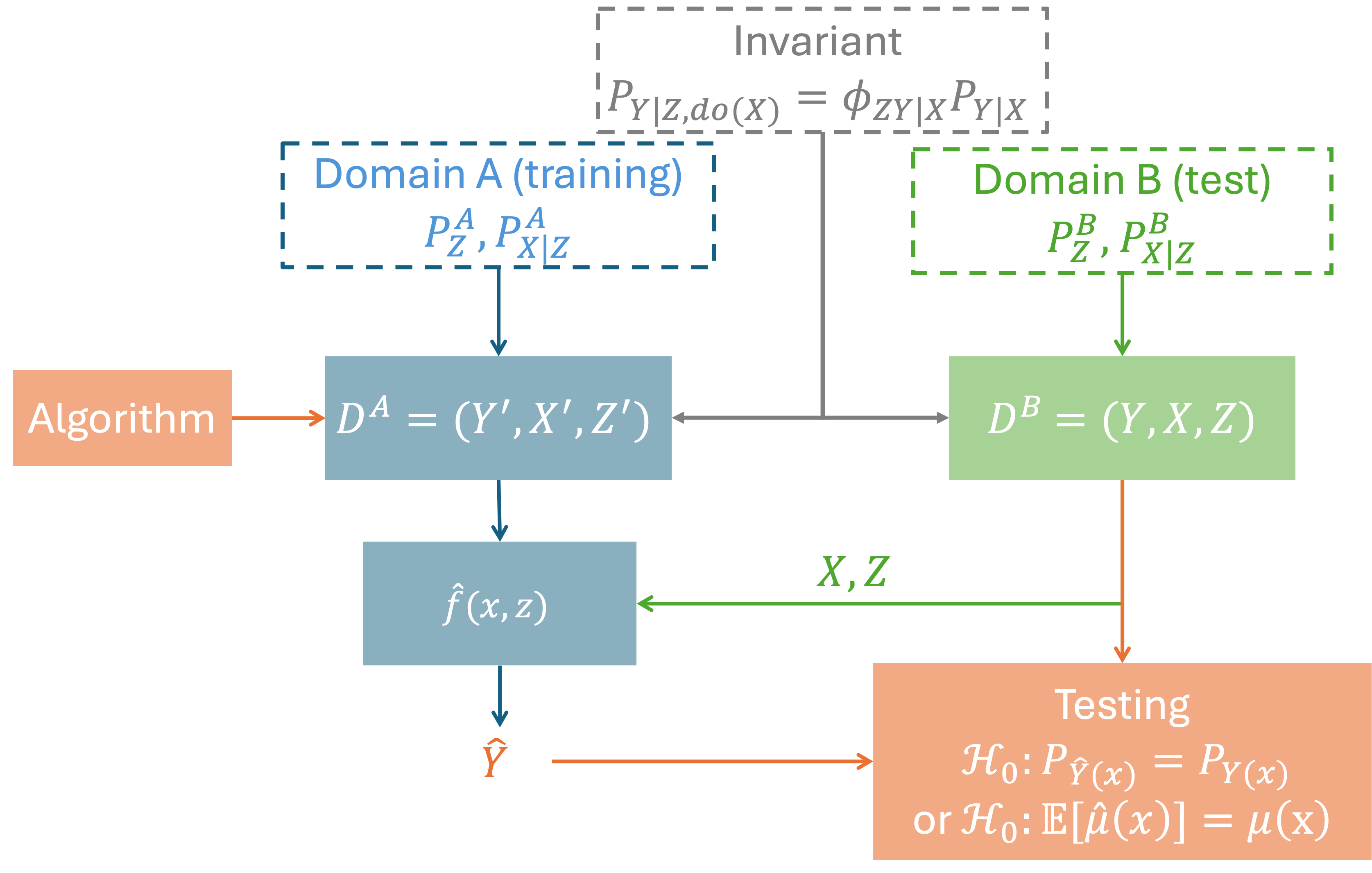
3 METHOD
Figure 1 provides an overview of our workflow. We begin by defining both a test and a training domain, each with a distribution over the pretreatment covariates and the treatment, allowing for distribution shifts across covariates and treatment allocation. The COD is frugally parameterized with a conditional copula, where the covariates’ cumulative distribution functions (CDFs) are derived from the test domain’s covariate densities. This ensures that samples from the test dataset follow a known, customizable marginal causal density, .
The training data is generated from the same COD but with a non-analytic marginal causal density, as the training covariate densities do not match the covariate CDFs used to parameterize the conditional copula. We then train a model, , on the training data. Finally, a statistical test is performed to validate whether the lower dimensional marginal quantity (e.g. ATE, , or the expected potential outcome, ) estimated using model outcomes equals the ground truth in the test domain.
3.1 Data Simulation
In this section we discuss how we can simulate the data. We show how we can construct two datasets with covariate/treatment domain shift with the exact same COD, but where in one domain the marginal causal effect is well understood.
3.1.1 Multi-domain Simulation with Frugal Models
We begin by specifying two data generating processes: the training data, , and the test data, . Our goal is to construct a COD that parameterizes the joint density across both domains, while ensuring that the marginal causal density in domain is parameterized by .
Recall from Section 2.2 that a general observational density can be factorized into the past, , and the COD, :
| (4) | ||||
where is the CDF associated with the marginal causal density .
Note that the copula density in Equation 4 is not only determined by the copula’s family and its parameterization, but also by the choice of marginal CDFs for the covariates, . If the conditional copula density is marginalized over the densities corresponding to the covariate CDFs, then the ranks of the marginal causal density will be uniformly distributed:
| (5) |
However, this uniformity is guaranteed only if the marginal covariate densities correspond to the CDFs used to parameterize the copula. If we instead consider a set of alternative marginal densities, , are not derived from the CDFs within the copula, i.e. then the rank uniformity is not assured. Thus, the COD density is generally valid under any distribution of the past, and will not in guarantee the sampling from the specified marginal causal density if the covariate densities are derived from the CDFs that parameterize the copula. We present the conditions by which alternative distributions will yield samples drawn from the specified marginal causal density, assuming that the conditional copula density is Gaussian in the Supplementary Material. Given how rarely these conditions are satisfied, we do not believe this will commonly be encountered in semi-synthetic benchmark generation. These conditions will likely be even harder to satisfy if a more complex multivariate copula (such as non-Gaussian vine) is chosen.
For evaluating generalization, we set the CDFs within the copula density to be derived from the covariate densities in the test domain . This allows us to construct the COD density across all covariate spaces,
| (6) | ||||
which will sample from a known marginal causal density equal to if the covariate CDFs in the copula are derived from the test domain covariate densities.
This offers a great deal of flexibility in testing method generalizability. One can draw training and test datasets with different covariate densities and propensity scores, while guaranteeing that the CODs remain consistent, and that the test data is drawn from a distribution with a marginal causal density parameterized by .
3.1.2 Generating Semi-Synthetic Benchmarks
In real-data based simulations, we follow the workflow outlined in Algorithm 1. First, we estimate the empirical CDFs of the pretreatment covariates for the test data, denoted as . We then estimate the marginal causal density and the joint copula , capturing the covariate-outcome dependency conditional on treatment. With the test copula known, we draw samples , and use inverse transforms to generate the covariate samples . Next, we estimate the propensity score model for the test data, and sample the treatment variable . The outcome for the test data calculating using , where is the sampled outcome rank from the copula. For the training data, we follow a similar approach. Details can be found in Algorithm 1.
3.2 Statistical Testing
Given that we know the marginal causal density parameterized by from the frugal parameterization, we are able to develop the statistical testing on instead of to for mean regression models, and instead of for distributional regression.
Our testing algorithms require some parameters: as the number of bootstrap samples, , as the number of samples simulated from training domain and test domain for each bootstrap, respectively; for distributional testing, we also need to specify , which is the number of outcome samples simulated from distributional regression output for each . We provide testing methods for two types of regression models: mean regression in Algorithm 2 or distributional regression in Algorithm 3. Note that, in Algorithm 2, we can replace with as the reference target when is binary, which is what we used in our experiments. The testing method used in Algorithm 3 can also be replaced by other statistical tests, e.g. Maximum Mean Discrepancy Test (Gretton et al.,, 2012) and Cramér-von Mises Test (Anderson,, 1962).
A summary of this workflow is presented in Figure 1.
4 EXPERIMENTS
In this section, we use our workflow to evaluate the generalizability of a range of modern causal models.
As discussed in several review papers like Curth et al., (2021), Ling et al., (2022) and Kiriakidou and Diou, (2022), methods such as Meta-Learners (e.g. T- and S-learners) (Künzel et al.,, 2019), CausalForest (Wager and Athey,, 2018), TARNet (Shalit et al.,, 2017), and BART (Chipman et al.,, 2010) are widely used for CATE estimation, each offering advantages in different scenarios. Our evaluation focuses on their performance under covariate distribution shifts, specifically examining the accuracy of their CATE estimations. Further details can be found in the Supplementary Material.
Another interesting algorithm to be evaluated is engression, introduced in Shen and Meinshausen, 2023b . It approximates the conditional distribution using a pre-additive noise model. Targeting at a distributional regression, the model is capable of extrapolating to unseen or underrepresented data points through its learned non-linear transformations. The key factors which affect engression’s generalizability are the distances between two domains, and whether the true underlying function must be strictly monotonic in the extrapolation region. In our experiments, we evaluate engression in both the S-learner and T-learner settings.
4.1 Synthetic Data
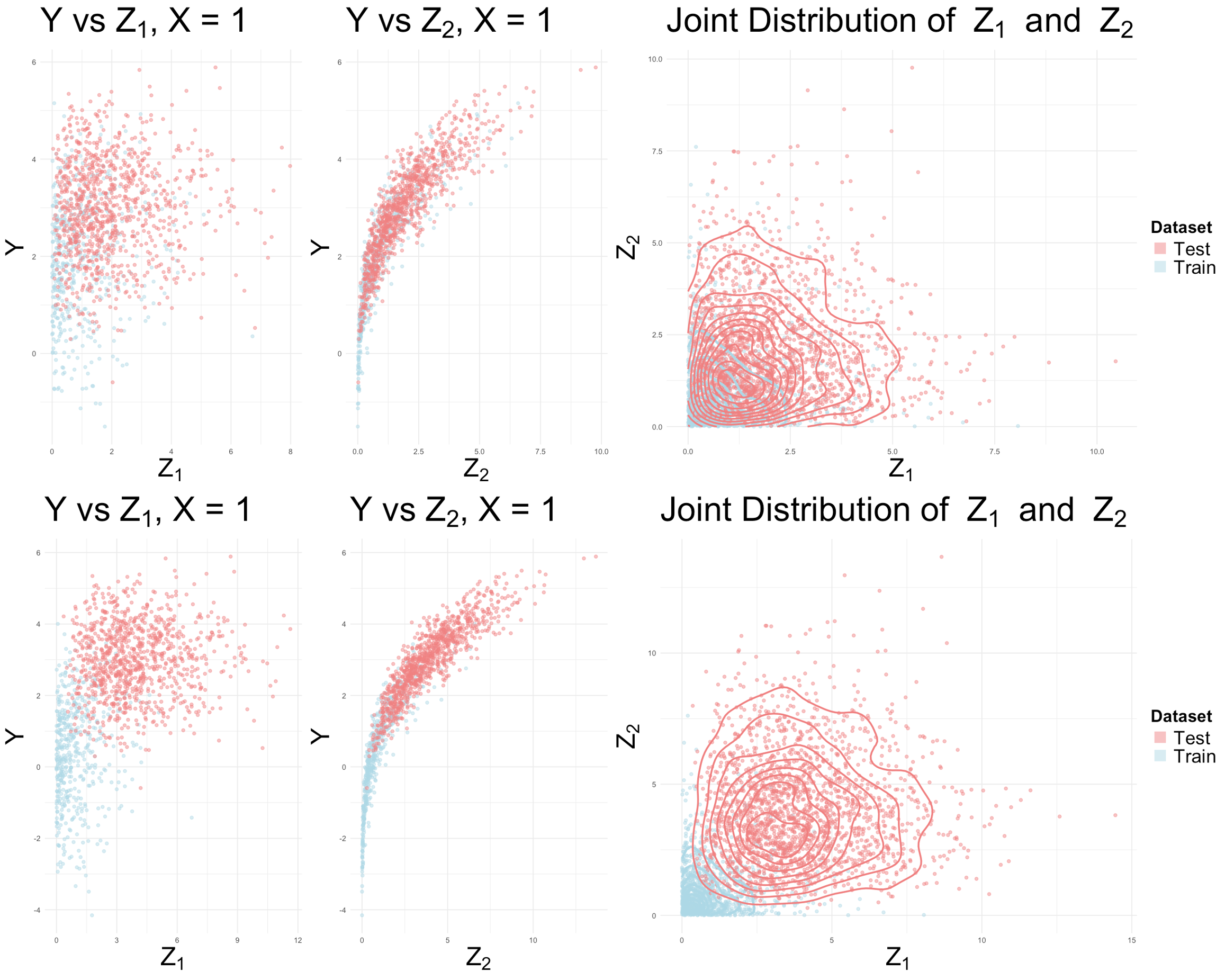
We first conduct experiments on synthetic data to demonstrate and validate our method. While our approach can handle various data types and is particularly effective with high-dimensional covariates and continuous treatment interventions, for clarity, in this simple example, we focus on two continuous confounders, and , sampled from identical gamma distributions, with a binary intervention . We first focus on a randomized controlled trials (RCT) setting, . Note that these parameters can be different between the two domains; here we just make them identical for simplicity in this experiment. We parameterize the Gaussian copula, , with Spearman correlation coefficients , and . The causal effect, is defined as in the test domain. For the simulation, we generate training samples and test samples per bootstrap, with bootstraps in total, repeating this process for 50 iterations. The marginal distributions of and in training domain follow identical Gamma distributions with shape and rate .
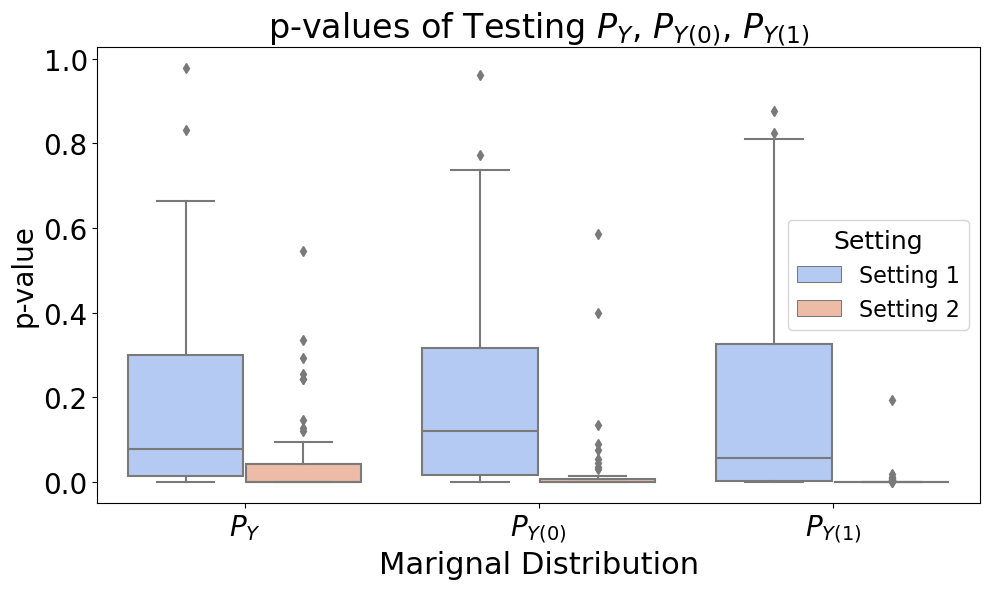
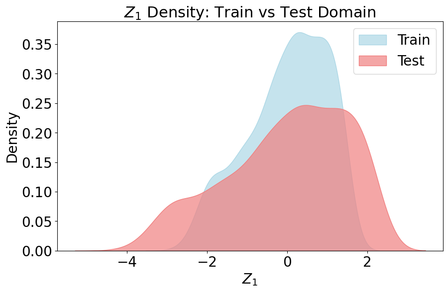
We examine two settings: in Setting 1, the test domain has a slight covariate shift, with and following a Gamma distribution of , . In Setting 2, the shift is more significant (, ). Despite these shifts, the COD remains the same due to frugal parameterization, as shown in Figure 2.
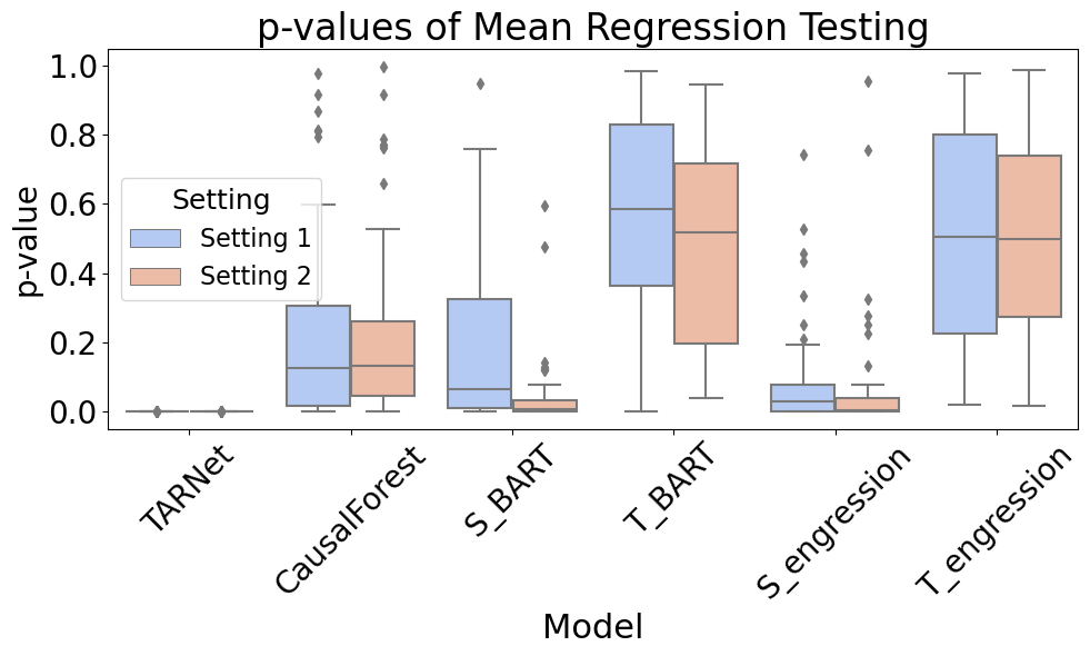
The p-values in Figure 3 illustrate the differences across models. As expected, with a more significant domain shift in Setting 2, models face greater difficulty in generalizing, as reflected by the smaller p-values generally compared to Setting 1. T-BART and T-engression showed good generalizability performances in this specific setting. TARNet struggles, likely due to the complexity of its representation learning network design and hyperparameter tuning.
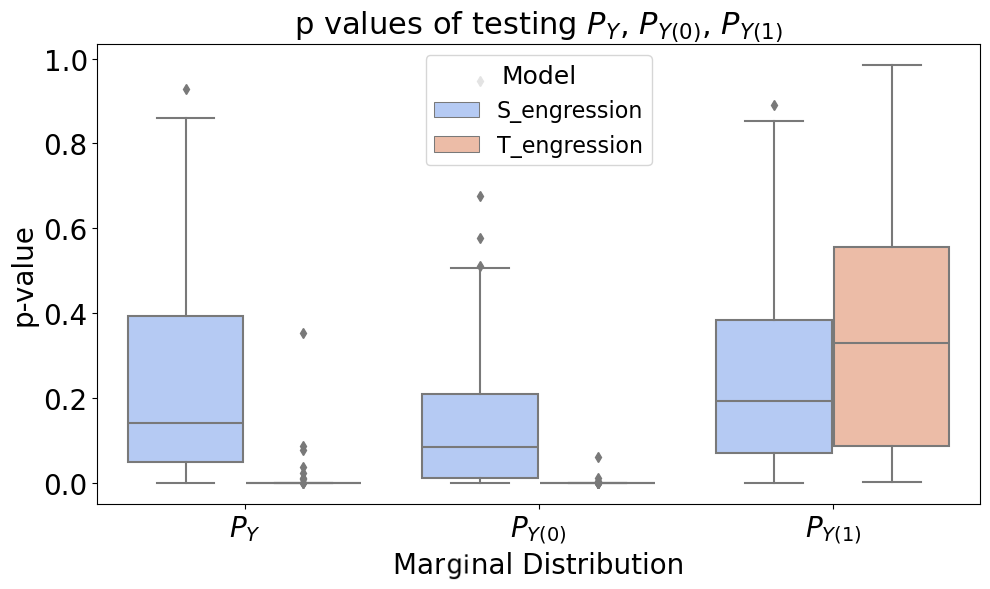
With our method, we are able to test the generalizability of distributional regression. Figure 4 demonstrates the p-values of distributional regression testing of S-engression under the two settings, with . Not surprisingly, since the covariate distribution shift in Setting 1 is smaller, S-engression demonstrates good generalizability compared to that in Setting 2.
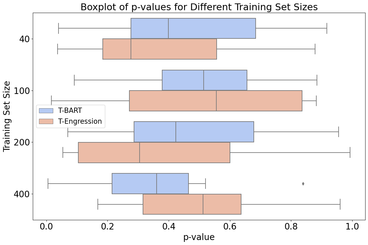
Supported by flexible simulations based on actual data, our method is useful for stress testing and model diagnostics. Figure 5 illustrates an example where we examine how varying the training set size affects the generalizability of T-BART and T-engression. The generalizability performances of T-BART and T-engression worsen as exceeds 100. This issue may stem from problems like overfitting, but solving these problems is not our focus. Rather, our method serves as a tool to detect and highlight potential issues when making predictions on real data, which is feasible with the simulation based on actual data using the frugal parameterization.
Note that extrapolation performance for models like engression is typically evaluated visually, one dimension at a time. Our method, however, offers significant advantages by providing statistical evaluation of extrapolation performance in high-dimensional covariates.
4.2 Real Data
We evaluate algorithm generalizability using the Infant Health and Development Program (IHDP) dataset, a randomized experiment conducted between 1985 and 1988 to study the effect of home visits on infants’ cognitive test scores (Hill,, 2011). This dataset has become widely used in domain adaptation research (Johansson et al.,, 2018; Curth et al.,, 2021; Shi et al.,, 2021).
The IHDP dataset contains trials, each consisting of the same 747 subjects and 25 covariates, with the first six being continuous and the rest binary. The potential outcomes and are provided in the data. In each trial , , , and is randomly chosen from a set of vectors. Thus, the potential outcomes vary across trials, while the covariates, CATE and ATE remain constant.
We first demonstrate algorithm generalizability by treating both domains as RCTs, i.e. setting the propensity score model as for all units. The observed outcome is then . We randomly select 50 trials from the 1000 available, with each trial used to create one training-test pair, and evaluate the model’s generalizability on them. To introduce domain shift, we keep all covariate values identical between the training and test domains, except for , which is set to 1.5 times the original value in the test domain compared to the training domain. For each training-test pair, we learn the parameters following Algorithm 1, specifying the marginal causal distribution to follow a Gamma distribution. We denote the resulting data generation distributions as for the training and test domains, respectively. We sample training data of from , and test data from . The number of bootstraps is set to be .
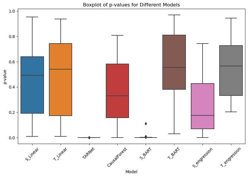
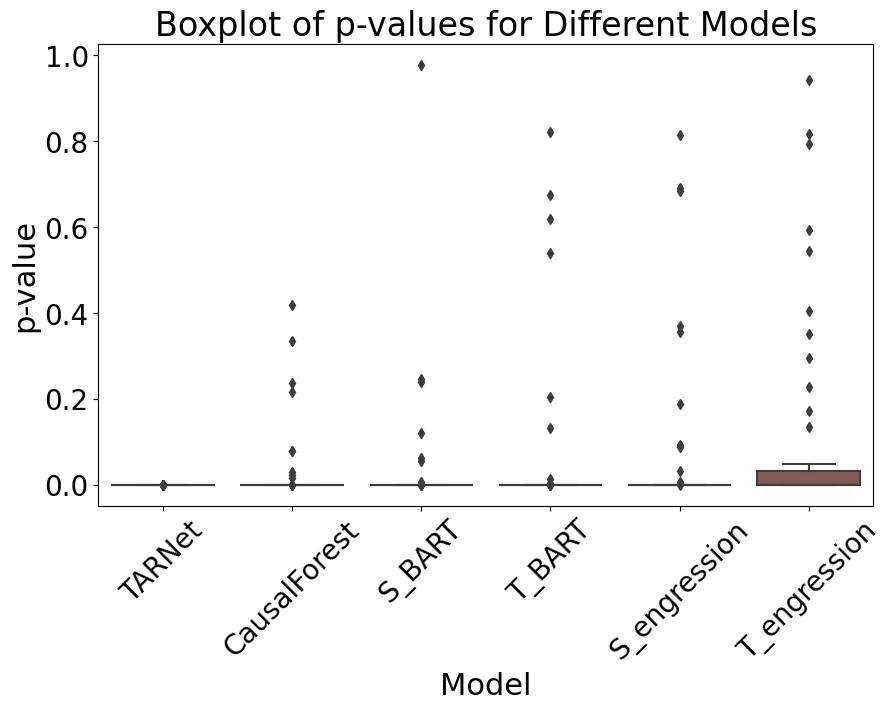
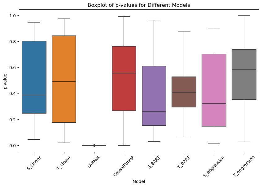
Figure 7 shows the boxplot of p-values of each model and Table 1 contains the percentage of values greater than 0.05 across the trials. T-/S-engression demonstrate better generalizability in this setting among all these methods. We also give the result of distributional regression testing in Figure 8.
| Model | RCT | Non-RCT |
|---|---|---|
| TARNet | 0 | 0 |
| CausalForest | 12% | 6% |
| S-BART | 12% | 8% |
| T-BART | 12% | 6% |
| S-engression | 18% | 6% |
| T-engression | 24% | 8% |
While we use the RCT setting as an example above to demonstrate our method, it is also applicable to observational studies. The percentage of across 50 trials of each algorithm, when treatment arms are imbalanced in each trial by setting can be found in Table 1. Since our paper’s focus is on providing a systematic generalizability evaluation method, we omit further analysis here.
Details on hyperparameters and additional experiments, including performance comparisons with or without domain shift when the CATE is known to be linear, are provided in the Supplementary Material.
5 SUMMARY
In this paper, we develop a statistical method for evaluating the generalizability of causal inference algorithms using actual application data, facilitated by frugal parameterization. Our approach introduces a semi-synthetic simulation framework that bridges the gap between synthetic simulations and real-world applications, supporting the generalizability evaluation of both mean and distributional regression models. Through flexible, user-defined data generation processes, our framework provides robust statistical testing to assess how well models trained in one domain generalize to shifted domains.
Through experiments on the synthetic and IHDP datasets, we assess the generalizability of algorithms such as TARNet, CausalForest, S-/T-BART, S-/T-engression under domain shift. Our method acts as a valuable diagnostic tool, allowing us to explore how factors like training set size or covariate shifts impact generalizability. These insights can help identify model strengths and weaknesses and inform how causal inference models adapt to different settings.
We remark that our approach of rejecting the null hypothesis shows that a model is not generalizable, but it does not quantify the extent of failure. An extention of this approach may be to develop a more flexible testing method, inspired by equivalence testing (Wellek,, 2002). This would assess not just whether a model fails but also by how much, determining if its performance is significantly worse than a given threshold. This offers a more nuanced view than traditional hypothesis testing. In this paper, we only consider marginal causal quantities as the validation references, but our framework can be easily adapted to use lower dimensional CODs as the reference instead.
We hope that this work inspires a more careful consideration of model evaluation, encourages simulations that better reflect real-world conditions, and highlights the importance of stress testing in advancing causal inference methodologies.
Acknowledgements
The authors would like to thank Laura Battaglia and Xing Liu for their helpful comments on the paper.
D.d.V.M is supported by a studentship from the UK’s EPSRC’s Doctoral Training Partnership (EP/T517811/1). L.Y. is supported by the EPSRC Centre for Doctoral Training in Modern Statistics and Statistical Machine Learning (EP/S023151/1) and Novartis.
References
- Anderson, (1962) Anderson, T. W. (1962). On the distribution of the two-sample cramer-von mises criterion. The Annals of Mathematical Statistics, pages 1148–1159.
- Bareinboim and Pearl, (2016) Bareinboim, E. and Pearl, J. (2016). Causal inference and the data-fusion problem. Proceedings of the National Academy of Sciences, 113:7345–7352.
- Bica and Schaar, (2022) Bica, I. and Schaar, M. (2022). Transfer learning on heterogeneous feature spaces for treatment effects estimation. In Advances in Neural Information Processing Systems, volume 35, pages 37184–37198.
- Bishop and Nasrabadi, (2006) Bishop, C. M. and Nasrabadi, N. M. (2006). Pattern recognition and machine learning, volume 4. Springer.
- Buchanan et al., (2018) Buchanan, A. L., Hudgens, M. G., Cole, S. R., Mollan, K. R., Sax, P. E., Daar, E. S., Adimora, A. A., Eron, J. J., and Mugavero, M. J. (2018). Generalizing evidence from randomized trials using inverse probability of sampling weights. Journal of the Royal Statistical Society Series A: Statistics in Society, 181(4):1193–1209.
- Caron et al., (2022) Caron, A., Baio, G., and Manolopoulou, I. (2022). Estimating individual treatment effects using non-parametric regression models: A review. Journal of the Royal Statistical Society Series A: Statistics in Society, 185(3):1115–1149.
- Chipman et al., (2010) Chipman, H. A., George, E. I., and McCulloch, R. E. (2010). BART: Bayesian additive regression trees.
- Curth et al., (2021) Curth, A., Svensson, D., Weatherall, J., and Schaar, M. (2021). Really doing great at estimating CATE? a critical look at ML benchmarking practices in treatment effect estimation. In Thirty-fifth Conference on Neural Information Processing Systems Datasets and Benchmarks Track (Round 2).
- Czado, (2019) Czado, C. (2019). Analyzing dependent data with vine copulas. Lecture Notes in Statistics, Springer.
- Dahabreh et al., (2019) Dahabreh, I. J., Robertson, S. E., Tchetgen, E. J., Stuart, E. A., and Hernán, M. A. (2019). Generalizing causal inferences from individuals in randomized trials to all trial-eligible individuals. Biometrics, 75(2):685–694.
- Dorie et al., (2024) Dorie, V., Chipman, H., and McCulloch, R. (2024). dbarts: Discrete Bayesian Additive Regression Trees Sampler. R package version 0.9-28.
- Evans and Didelez, (2024) Evans, R. and Didelez, V. (2024). Parameterizing and simulating from causal models. Journal of the Royal Statistical Society Series B: Statistical Methodology, 86:535–568.
- Gretton et al., (2012) Gretton, A., Borgwardt, K. M., Rasch, M. J., Schölkopf, B., and Smola, A. (2012). A kernel two-sample test. The Journal of Machine Learning Research, 13(1):723–773.
- Hill, (2011) Hill, J. L. (2011). Bayesian nonparametric modeling for causal inference. Journal of Computational and Graphical Statistics, 20(1):217–240.
- Johansson et al., (2018) Johansson, F., Kallus, N., Shalit, U., and Sontag, D. (2018). Learning weighted representations for generalization across designs. arXiv preprint arXiv:1802.08598.
- Johansson et al., (2016) Johansson, F., Shalit, U., and Sontag, D. (2016). Learning representations for counterfactual inference. In International Conference on Machine Learning, pages 3020–3029.
- Kern et al., (2016) Kern, H. L., Stuart, E. A., Hill, J., and Green, D. P. (2016). Assessing methods for generalizing experimental impact estimates to target populations. Journal of Research on Educational Effectiveness, 9(1):103–127.
- Kiriakidou and Diou, (2022) Kiriakidou, N. and Diou, C. (2022). An evaluation framework for comparing causal inference models. In Proceedings of the 12th Hellenic Conference on Artificial Intelligence, pages 1–9.
- Künzel et al., (2019) Künzel, S. R., Sekhon, J. S., Bickel, P. J., and Yu, B. (2019). Metalearners for estimating heterogeneous treatment effects using machine learning. Proceedings of the National Academy of Sciences, 116(10):4156–4165.
- Ling et al., (2022) Ling, A., Montez-Rath, M., Carita, P., Chandross, K., Lucats, L., Meng, Z., Sebastien, B., Kapphahn, K., and Desai, M. (2022). A critical review of methods for real-world applications to generalize or transport clinical trial findings to target populations of interest. arXiv preprint arXiv:2202.00820.
- Microsoft Research, (2019) Microsoft Research (2019). EconML: A Python Package for ML-Based Heterogeneous Treatment Effects Estimation. https://github.com/microsoft/EconML.
- Pearl, (2009) Pearl, J. (2009). Causality. Cambridge University Press.
- Rüschendorf, (2009) Rüschendorf, L. (2009). On the distributional transform, Sklar’s theorem, and the empirical copula process. Journal of Statistical Planning and Inference.
- Shalit et al., (2017) Shalit, U., Johansson, F. D., and Sontag, D. (2017). Estimating individual treatment effect: generalization bounds and algorithms. In International Conference on Machine Learning, pages 3076–3085. PMLR.
- (25) Shen, X. and Meinshausen, N. (2023a). engression: Engression Modelling. R package version 0.1.4.
- (26) Shen, X. and Meinshausen, N. (2023b). Engression: Extrapolation for nonlinear regression? arXiv preprint arXiv:2307.00835.
- Shi et al., (2021) Shi, C., Veitch, V., and Blei, D. (2021). Invariant representation learning for treatment effect estimation. In Uncertainty in Artificial Intelligence, pages 1546–1555.
- Sklar, (1959) Sklar, M. (1959). Fonctions de répartition à dimensions et leurs marges. In Annales de l’ISUP.
- Wager and Athey, (2018) Wager, S. and Athey, S. (2018). Estimation and inference of heterogeneous treatment effects using random forests. Journal of the American Statistical Association, 113(523):1228–1242.
- Wellek, (2002) Wellek, S. (2002). Testing statistical hypotheses of equivalence. Chapman and Hall/CRC.
- Yu et al., (2024) Yu, H., Liu, J., Zhang, X., Wu, J., and Cui, P. (2024). A survey on evaluation of out-of-distribution generalization. arXiv preprint arXiv:2403.01874.
- Zhou et al., (2022) Zhou, K., Liu, Z., Qiao, Y., Xiang, T., and Loy, C. C. (2022). Domain generalization: A survey. IEEE Transactions on Pattern Analysis and Machine Intelligence, 45:4396–4415.
Supplementary Materials
Appendix A COPULA BACKGROUND
Copulas present a powerful tool to model joint dependencies independent of the univariate margins. This aligns well with the requirements of the Frugal Parameterisation, where dependencies need to be varied without altering specified margins (the most critical being the specified causal effect). Understanding the constraints and limitations of copula models ensures that causal models remain accurate and consistent with the intended parameterisation.
A.1 SKLAR’S THEOREM
Sklar’s theorem (Sklar,, 1959; Czado,, 2019) provides the fundamental foundation for copula modelling by providing a bridge between multivariate joint distributions and their univariate margins. It allows one to separate the marginal behaviour of each variable from their joint dependence structure, with the latter being the copula itself.
Theorem 1.
For a d-variate distribution function , with univariate margin , the copula associated with is a distribution function with uniform margins on that satisfies
-
1.
If F is a continuous d-variate distribution function with univariate margins and rank functions then
-
2.
If is a d-variate distribution function of discrete random variables (more generally, partly continuous and partly discrete), then the copula is unique only on the set
The copula distribution is associated with its density
where is the univariate density function of the variable.
Note that Sklar’s theorem explicitly refers to the univariate marginals of the variable set to convert between the joint of univariate margins and the original distribution . For absolutely continuous random variables, the copula function is unique. This uniqueness no longer holds for discrete variables, but this does not severely limit the applicability of copulas to simulating from discrete distributions.
An equivalent definition (from an analytical purview) is is a -dimensional copula if it has the following properties:
-
1.
-
2.
.
-
3.
is -non-decreasing.
Definition 1.
A copula is -non-decreasing if, for any hyperrectangle , the -volume of is non-negative.
A.2 COPULAS FOR DISCRETE VARIABLES
A.2.1 CHALLENGES AND MOTIVATIONS
Modelling the dependency between discrete and mixed data is particularly challenging as copulas for discrete variables are not unique. Additionally, copulas encode a degree of ordering in the joint as probability integral transforms are inherently ranked, and hence should only be used for count or ordinal data models. We use the approach suggested by Rüschendorf, (2009). An outline of this method is presented in Section A.2.2.
A.2.2 EMPIRICAL COPULA PROCESSES FOR DISCRETE VARIABLES
In order to deal with discrete variables, we use a the Generalised Distributional Transform of a random variable found originally proposed by Rüschendorf, (2009). We quote the main result from Rüschendorf, (2009) below.
Theorem 2.
On a probability space let be a real random variable with distribution function and let be uniformly distributed on and independent of . The modified distribution function is defined by
We define the (generalised) distributional transform of by
An equivalent representation of the distributional transform is
Rüschendorf, (2009) makes a key remark about the generalised transform’s lack of uniqueness for discrete variables. Such a dequantisation step may introduce artificial local dependence which may lead to an incorrect flow being inferred, and therefore hinder the inference of the causal margin.
Appendix B GAUSSIAN COPULA WITH GAUSSIAN MARGINS
In the main text, we generate synthetic data from a Gaussian copula with univariate Gaussian margins. The resultant joint multivariate density is a multivariate Gaussian. Consequently, any univariate density conditioned on all the other variables will be Gaussian, and the conditional mean is a linear function of the conditioning variables. The proof for the latter can be found in Bishop and Nasrabadi, (2006). The proof for the former is provided below.
Theorem 3.
Let be a set of univariate Gaussian random variables, where each . Let denote a multivariate Gaussian copula parameterized by a correlation matrix . The joint distribution of the random vector is multivariate normal, specifically:
where is the mean vector, and is a diagonal matrix with for , and for .
Proof.
Consider a Gaussian copula with univariate Gaussian marginals , where each . Let the copula distribution function be given by
where is the CDF of the -dimensional standard normal distribution with correlation matrix , and is the CDF of the standard normal distribution. The corresponding density function is:
where is the density of and is the copula density. To compute the copula density, we differentiate with respect to :
Using the Gaussian copula formula, we obtain:
where is the PDF of the multivariate normal distribution with mean zero and correlation matrix , and is the standard univariate normal PDF.
Next, recall that for any Gaussian random variable , we have:
By Lemma 4 (below), the inverse CDF of the standard normal, , satisfies:
Therefore, substituting into the copula density, we get:
Now, combining this with the marginal densities, we obtain the joint density:
Finally, multiplying by the product of the univariate densities gives:
which is the PDF of a multivariate Gaussian distribution with mean vector and covariance matrix . Hence, the joint distribution of is multivariate normal, as desired. ∎
Lemma 4.
Let denote the inverse CDF of the standard normal distribution. For a Gaussian random variable , we have:
Proof.
This follows by noting that , and thus:
∎
Appendix C DERIVING UNIFORMLY MARGINAL RANKS USING A GAUSSIAN COPULA
In this section we outline the circumstances by where two different sets of marginal covariate distributions may yield the same marginal causal effect densities when assuming that is a conditional copula density derived from a Gaussian copula. First and foremost, we want to emphasize that this is a rather strict scenario, and it is less likely to occur in real-world settings.
This assumes that the ranks of the marginal causal effect are distributed as follows:
| (7) |
which assures that the marginal distribution of if . Given Equation 7, our question is whether there is another set of conditioning variables which yields the same marginal outcome of the conditional model.
We can rewrite Equation 7 as a linear combination of Gaussians:
| (8) |
where , and are an arbitrary set of conditioning variables. If the marginal distribution of is Gaussian, then must each be Gaussian (Gaussian closure under linear marginalisation).
Our next question is finding which linear transformations of will yield a standard Gaussian distribution of . Assume that yields a marginal distribution of which is standard Gaussian. Let us perform the change of variables transformation
where and are all constants. Our goal is to identify a set of conditions for whereby
Starting with the expectation,
| (9) | ||||
| (10) |
Similarly for the variance,
| (11) | ||||
| (12) |
The set of variables by which we can exactly sample from the same marginal effect are if
for any if
This is indeed an extreme case. Given how rarely these conditions are satisfied, especially in high-dimensional settings where the copula function can become quite complex, it is not a significant concern for our work.
Appendix D MODELS
We provide details of the models evaluated in our paper.
Engression
Engression proposed in Shen and Meinshausen, 2023b approximates the conditional distribution using a pre-additive noise model , where is a non-linear function that captures non-linear relationships and introduces flexible noise. Built on the neural network architecture that efficiently learns this structure, it optimizes the energy score loss for accurate distributional regression.
Meta-learners
Meta-learners are flexible frameworks in causal inference designed to estimate individualized treatment effects by leveraging machine learning models. Two common types are T-learners and S-learners. Details can be found in Künzel et al., (2019).
T-learners work by training separate models for the treated and untreated groups, predicting outcomes under each treatment condition, and then calculating the difference between these predictions to estimate the treatment effect. S-learners combine both treated and untreated data into a single model by including treatment as an input feature, allowing the model to learn the outcome function across both treatment conditions simultaneously. These learners provide a modular approach to estimating Conditional Average Treatment Effects (CATE) and can adapt to different settings and model complexities.
CausalForest
CausalForest is an extension of random forests designed to estimate heterogeneous treatment effects by partitioning the data into subgroups with similar treatment responses. Introduced by Wager and Athey, (2018), CausalForest uses a tree-based ensemble method to non-parametrically estimate Conditional Average Treatment Effects (CATE) by building separate models for different covariate regions, while ensuring a balance between treated and control units in each partition. This method is flexible and adapts to complex data structures, making it a powerful tool for understanding treatment effect heterogeneity.
BART
BART (Bayesian Additive Regression Trees), first introduced in Chipman et al., (2010), is a non-parametric machine learning method that uses an ensemble of regression trees to model complex relationships between covariates and outcomes. The BART model estimates the posterior distribution of the outcome by summing the contributions from many trees, each of which is trained to explain part of the residual error left by the others. This ensemble approach makes BART particularly effective at capturing complex, non-linear relationships between the covariates and the outcome. Unlike standard decision trees, BART applies a Bayesian framework, allowing it to quantify uncertainty in its predictions and avoid overfitting through regularization priors.
TARNet
TARNet (Treatment-Agnostic Representation Network), first introduced in Johansson et al., (2016), is a neural network-based model for estimating heterogeneous treatment effects in causal inference. It works by learning a shared representation of covariates, independent of treatment assignment, and then using this representation to estimate potential outcomes for both the treated and untreated groups. By focusing on treatment-agnostic representation learning, TARNet aims to improve the generalizability and accuracy of treatment effect estimates, particularly in high-dimensional settings.
Appendix E COMPUTATION DETAILS
We provide computation details in the Experiment section. We use default recommended hyperparameters for each model.
| Model | Key Hyperparameters | Package |
|---|---|---|
| TARNet | Number of layers = 2, batch size = 64, learning rate = 0.0001, number of epochs = 2000 | Python, catenets (Curth et al.,, 2021) |
| CausalForest | Number of trees = 100, maximum depth = 3 | Python, econml (Microsoft Research,, 2019) |
| S-/T-BART | Number of trees = 75, number of iterations = 4, number of burn-in iterations = 200, posterior draws = 800 | R, dbarts (Dorie et al.,, 2024) |
| S-/T-engression | Number of layers = 3, batch size = 64, learning rate = 0.01, number of epochs = 500 | Python, engression, (Shen and Meinshausen, 2023a, ) |
All experiments were conducted on a MacBook with an Apple M3 chip, 8-core CPU, and 32GB RAM. The codes can be found in TestGeneralizability.zip.
Appendix F ADDITIONAL EXPERIMENTS
We include an additional experiment we run in this section, which is based on the synthetic data setting in the main text, but without domain shift. We set the marginal distribution of , to be , and , . In this case, the CATE should be linear, as we mentioned in Appendix B.
Result of when there is no domain shift can be found in Figure 9. We see that the p-values of both S-LinearRegression and T-LinearRegression are uniformly distributed. Given the true CATE function is indeed linear, this result validates our proposed method.
We next test when there is domain shift, i.e., we keep all the settings the same as above for training set, but we change the marginal distribution of , in the test set to be . Figure 10 shows the results. Linear regressions still demonstrate good generalizability performances! However, generalizability of algorithms like S-engression and S-BART worsens, likely due to problems such as overfitting.