Accelerating Task Generalisation with Multi-Level Hierarchical Options

Abstract

Creating reinforcement learning agents that generalise effectively to new tasks is a key challenge in AI research. This paper introduces Fracture Cluster Options (FraCOs), a multi-level hierarchical reinforcement learning method that achieves state-of-the-art performance on difficult generalisation tasks. FraCOs identifies patterns in agent behaviour and forms options based on the expected future usefulness of those patterns, enabling rapid adaptation to new tasks. In tabular settings, FraCOs demonstrates effective transfer and improves performance as it grows in hierarchical depth. We evaluate FraCOs against state-of-the-art deep reinforcement learning algorithms in several complex procedurally generated environments. Our results show that FraCOs achieves higher in-distribution and out-of-distribution performance than competitors.

1 Introduction

A key goal of AI research is to develop agents that can leverage structured prior knowledge, either provided or learned, to perform competently in unfamiliar domains (Pateria et al.,, 2021). This is a common feature in animals; for example, many newborn mammals, such as foals, can walk shortly after birth due to innate motor patterns, while human infants display instinctive stepping motions when supported (Adolph and Robinson,, 2013; Dominici et al.,, 2011). These innate behaviours, shaped by evolution, act as priors that guide goal-directed actions and enable rapid adaptation.

In parallel, humans are believed to organise behaviours into a hierarchy of temporally extended actions, which helps break complex tasks into simpler, manageable steps (Rosenbloom and Newell,, 1986; Laird et al.,, 1987). For instance, human decision-making often involves planning with high-level actions like “pick up glass” or “drive to college,” each of which comprises subtasks such as “reach for glass” or “pull door handle.” These eventually decompose into basic motor movements.

This hierarchical fragmentation likely arises from sub-experiences of past tasks (Brunskill and Li,, 2014). Notably, parts of this hierarchy are shared between tasks; for instance, both “pick up glass” and “pull door handle” involve similar gripping movements. Such shared temporal actions may facilitate rapid learning of new tasks beyond those previously experienced. Replicating this hierarchy in algorithms could allow artificial agents to also adapt quickly (Heess et al.,, 2016).

Despite advances in hierarchical methods, generalising behaviours across diverse tasks remains a significant challenge for artificial agents (Cobbe et al.,, 2019). Many approaches struggle with effectively transferring skills to new environments, limiting their ability to adapt to real-world scenarios (Pateria et al.,, 2021).

In this paper, we make two key contributions:

1. We introduce Fracture Cluster Options (FraCOs), a novel framework for defining, forming, and utilizing multi-level hierarchical options based on their expected future usefulness.

2. We empirically demonstrate that FraCOs significantly enhances out-of-distribution (OOD) learning. Our method outperforms three baselines—Proximal Policy Optimization (PPO) (Schulman et al.,, 2017), Option Critic with PPO (OC-PPO) (Klissarov et al.,, 2017) and Phasic Policy Gradient (Cobbe et al.,, 2021)—in both in-distribution and OOD learning across several environments from the Procgen benchmark (Cobbe et al.,, 2020).

2 Background

2.1 Reinforcement Learning

Standard Reinforcement Learning (RL) focuses on how agents can “take actions in different states of an environment to maximize cumulative future reward", where the reward provides task-specific feedback (Sutton and Barto,, 2018). In any environment, an agent exists in a state $s$ and can perform an action $a$, both of which may be discrete, continuous, or multidimensional. Most RL problems are framed as a Markov Decision Process (MDP). An MDP is defined as a tuple $\langle S,A,P,R,\gamma\rangle$, where $S$ is the set of possible states, $A$ is the set of possible actions, $P$ is the transition probability function with $P(s,a,s^{\prime})$ indicating the probability of transitioning from state $s$ to $s^{\prime}$ after action $a$, $R$ is the reward function where $R(s,a,s^{\prime})$ gives the reward for transitioning from $s$ to $s^{\prime}$ via action $a$, and $\gamma\in[0,1]$ is the discount factor. An MDP assumes the Markov property, where the future state and reward depend only on the current state and action.

At each time step $t\geq 0$, the agent makes a decision based on its current state $s_{t}$ using a policy, denoted as $\pi(s_{t})$. The policy maps states to probabilities over actions, guiding the agent’s behaviour. The actions taken produce observed experience data of the form $(s_{t},a_{t},r_{t+1},s_{t+1})$. When the agent interacts with the environment until it reaches a termination state, the full sequence of observations is called a trajectory $T$. The objective of reinforcement learning is to learn a policy that maximises the cumulative discounted returns, defined as $G_{t}=\sum_{k=0}^{\infty}\gamma^{k}r_{t+k+1}$.

In this paper, we define an environment as the external system with which the agent interacts, characterized by $\langle S,A,P,R\rangle$. In our work, a task is defined as a unique MDP.

2.2 Hierarchical Reinforcement Learning

Hierarchical Reinforcement Learning (HRL) extends standard RL by organising decision-making into multiple levels of abstraction. A key paradigm in HRL is the options framework, which encapsulates extended sequences of actions into options (Sutton and Barto,, 2018). An option consists of an initiation set $I$, which defines the states where it can be selected, an intra-option policy $\pi_{\text{intra}}$, which governs the actions while the option is active, and a termination condition $\beta:S\rightarrow[0,1]$, which defines when the option ends. The intra-option policy executes actions until the termination condition $\beta(s)$ is satisfied.

Options operate within a Semi-Markov Decision Process (SMDP). An SMDP is an extension of an MDP where actions can have variable durations. The agent chooses between options and primitive actions at each decision point, with a policy over options, $\pi_{\text{opt}}$, deciding which to execute based on the current state. This hierarchical structuring can improve exploration and learning efficiency by enabling agents to plan over extended time horizons and break complex tasks into manageable sub-tasks. This decomposition reduces the decision space, facilitates structured exploration, and simplifies credit assignment, particularly in environments with sparse rewards (Sutton et al.,, 1999; Dayan and Hinton,, 1992).

2.3 Generalisation

Generalisation in Reinforcement Learning (RL) encompasses a broad class of problems (Kirk et al.,, 2021). These problems can be categorised based on the relationship between training and testing distributions, either falling within Independent and Identically Distributed (IID) scenarios or extending to Out-of-Distribution (OOD) contexts. Additionally, generalisation can be classified by the features of the environment that change, including the state space, observation space, dynamics, and rewards. This classification leads to eight possible combinations of generalisation challenges.

In this work, we define IID generalisation as the ability of agents to generalise within tasks drawn from the same distribution as their training tasks. In contrast, OOD generalisation refers to an agent’s ability in tasks that differ from those encountered during training.

We evaluate FraCOs’ generalisation performance in OOD tasks where the state space $S$ and reward function $R$ vary, while the action space $A$, transition dynamics $P$, and discount factor $\gamma$ remain constant. This setup reflects real-world scenarios where an agent, such as a robot, operates under fixed dynamics but faces diverse environments and goals.

3 Related Work

Policy transfer and single-level option transfer methods, aim to broaden an agent’s task-handling capabilities. Examples of policy transfer include works by Finn et al., (2017), Grant et al., (2018), Frans et al., (2017), Cobbe et al., (2021), and Mazoure et al., (2022). Option transfer methods, on the other hand, focus on learning a set of reusable options to enhance rewards in new situations (Konidaris and Barto,, 2007; Barreto et al.,, 2019; Tessler et al.,, 2017; Mann and Choe,, 2013). While a few methods in the literature explore multi-level hierarchies, they do not focus on option transfer as a mechanism for accelerating task adaptation and generalisation (Riemer et al.,, 2018; Evans and Şimşek,, 2023; Levy et al.,, 2017; Fox et al.,, 2017).

HRL has typically focused on addressing broader challenges such as long-term credit assignment and structured exploration (Dayan and Hinton,, 1992; Parr and Russell,, 1997; McGovern and Sutton,, 1998; Sutton et al.,, 1999). Two foundational paradigms within HRL are: 1) sub-goal-based approaches, which typically decompose tasks into smaller, state-based intermediate objectives, and 2) the options framework, which formalises temporally extended actions as options (Sutton et al.,, 1999). In both paradigms the ability to learn transferable abstractions at more than two levels of hierarchy is still an open research question (Pateria et al.,, 2021).

Recent work has proposed methods for forming and managing multi-level hierarchies. Levy et al., (2017) and Evans and Şimşek, (2023) introduce sub-goal-conditioned approaches for multi-level abstraction. However, due to their reliance on state-based-sub-goals, these methods face difficulties in sub-goal selection in complex state spaces such as pixel-based representations. Moreover, all state-based-sub-goal methods struggle to transfer sub-goals to different state spaces. Additionally, they do not account for the variability in action sequences required to transition between sub-goals; for example, “booking a holiday" could involve “calling a travel agent" or “using the internet," each demanding different skills. In contrast, FraCOs avoids creating state-based-sub-goals, providing a more flexible framework for transfer across state spaces.

Our work is more closely related to Hierarchical Option Critic (HOC) by Riemer et al., (2018) and the Discovery of Deep Options (DDO) by Fox et al., (2017), both of which use the options framework. DDO employs an expectation gradient method to construct a hierarchy top-down from expert demonstrations. However, DDO does not optimize for generality and it remains unclear how the discovered options perform in unseen tasks. Moreover, the reliance on demonstrations limits the development of more complex abstractions than those demonstrated. In comparison, FraCOs builds bottom-up, forming increasingly complex abstractions. FraCOs also selects options based on their expected usefulness in future tasks, directly addressing generalisation challenges.

HOC generalises the Option-Critic (OC) framework introduced by Bacon et al., (2017) to multiple hierarchical levels. HOC learns all options simultaneously during training. However, both OC and HOC suffer from option collapse, where either all options converge to the same behaviour or one option is consistently chosen (Harutyunyan et al.,, 2019). Moreover, OC methods introduce additional complexity to the learning algorithm, which has been shown to slow learning compared to non-hierarchical approaches like PPO (Schulman et al.,, 2017; Zhang and Whiteson,, 2019). Option selection within the FraCOs process naturally prevents option collapse, and has been shown to increase the rate of learning over baselines (see Section 5.3).

4 Fracture Cluster Options

We hypothesise that identifying reoccurring patterns in an agent’s behaviour across successful tasks will improve performance on future, unseen tasks. Our method consists of three key stages: 1) Identifying the underlying reoccurring patterns in an agent’s behaviour across multiple tasks, 2) selecting the most useful patterns—those likely to appear in successful trajectories of all possible tasks, and 3) defining these identified patterns as options for the agent’s future use.

4.1 Identifying Patterns in Agent Behaviour

We seek to identify and cluster reoccurring patterns of states and actions in agent behavior. To achieve this, we introduce the concept of fractures. A fracture is defined as a state $s_{t}$ paired with a sequence of subsequent actions. The length of this action sequence is determined by a parameter known as the chain length $b$, which specifies the number of actions following the state $s_{t}$. More formally, a fracture is represented as:

$$\phi=(s_{t},a_{t},a_{t+1},\dots,a_{t+b-1})$$ (1)

where $a_{t},a_{t+1},\dots,a_{t+b-1}$ represent the subsequent actions from $s_{t}$. The parameter $b$ controls the temporal extent of the fracture.

We can derive fractures from the trajectories of tasks which an agent has experienced. Consider a trajectory of length $n$. The set of fractures $F$ derived from this trajectory is defined as:

$$F=\{(s_{t},a_{t},a_{t+1},\dots,a_{t+b-1})\mid 0\leq t\leq n-b\}.$$ (2)

For a set of trajectories $\mathcal{T}$, we derive fractures from each individual trajectory. The complete set of fractures from all trajectories is denoted by $\Phi=\{F_{1},F_{2},\dots,F_{|T|}\}$. Individual trajectories are denoted by $\tau$, with $\tau\in\mathcal{T}$.

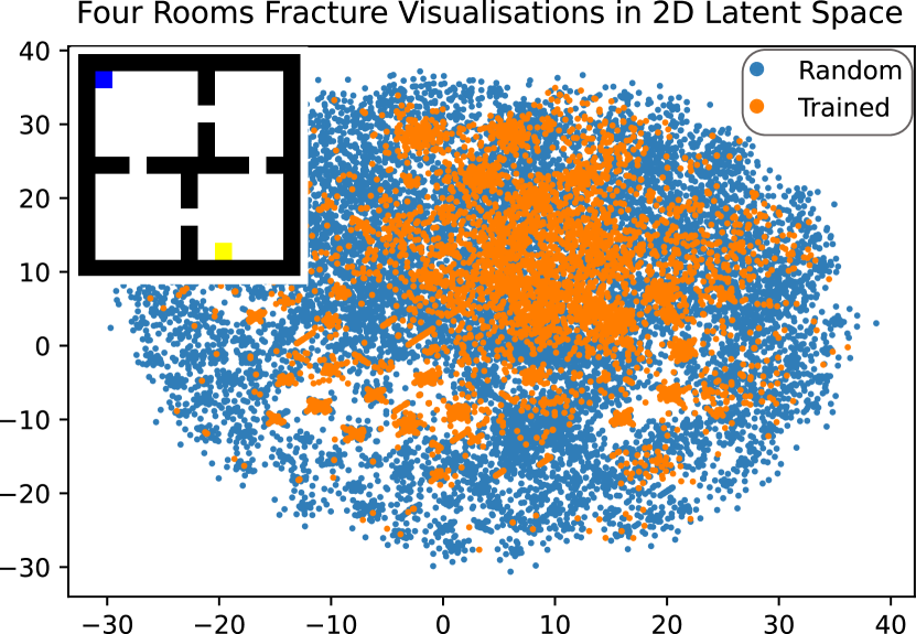
Figure 1: A two-dimensional representation of the fractures ($b=2$) formed by agents acting for 10,000 steps in the Four Rooms environment.

We investigate whether fractures capture underlying structure by first identifying them in the Four Rooms environment. Four Rooms is a classic grid-based reinforcement learning environment, consisting of four connected rooms separated by walls with narrow doorways. The agent’s objective is to navigate through the rooms to reach a specified goal, receiving a reward for reaching this goal. Four Rooms is depicted in the top left corner of Figure 1, see Appendix A.7 for more detail. In all of our grid-world implementations, the agent can observe only a 7x7 area centered on itself and a scalar indicating the direction of the reward. This is similar to MiniGrid, except that our observations are ego-centric (Chevalier-Boisvert et al.,, 2023).

We train a tabular Q-learning agent to solve multiple different reward locations in Four Rooms and generate trajectories for both the trained agent and a random agent. Fractures are then created following Equation 2, with $b=2$. To reveal the structural differences between the fractures of the random agent and the trained agent, we use UMAP (McInnes et al.,, 2018), a dimension reduction technique that projects the high-dimensional fracture data into a two-dimensional space. UMAP is particularly useful for this task because it preserves local similarities within the data. We plot the resulting two-dimensional visualization in Figure 1. This highlights a near-uniform distribution for the random agent, while the trained agent’s fractures form distinct clusters, reflecting underlying behaviour structures. This phenomenon is consistent across other environments (see Appendix A.7.4).

We employ unsupervised clustering techniques to identify and formalise the fracture clusters, denoted as $\phi_{c}$. Specifically, we use HDBSCAN for all tabular methods in this work (Campello et al.,, 2013). Fractures with a chain length of $b=4$ are grouped into clusters, and four clusters are randomly selected for visualisation in Figure 2. Each visualisation shows all fractures within a cluster, demonstrating that, despite differences in starting states, action sequences, and terminal states, the fractures within each cluster share similar semantic meanings.

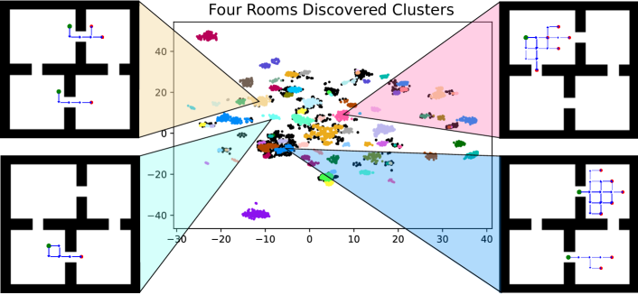
Figure 2: Four examples of discovered fracture clusters ($b=4$) within the Four Rooms environment. The graph represents fracture clusters of a trained agent in the Four Rooms environment, colours are used to visualise cluster boundaries. In the four examples, the green point represents possible starting states, blue arrows indicate actions, the width of the arrows shows the frequency of the state-action pair within the cluster, and the red point indicates possible terminal states.

4.2 Selecting Useful Fracture Clusters

In Section 4.1 fracture clusters are formed based on behaviour similarity; however, the number of potential clusters can be extensive, with some being highly task-specific. Selecting all clusters as options may burden the agent with unnecessary choices. Therefore, it is essential to identify the most useful clusters—those likely to appear in future tasks.

First, consider the hypothetical scenario in which we can observe all possible trajectories across all possible tasks. In this ideal setting, the set of all successful fractures, denoted as $\Phi_{s}$, would be derived from fractures within the successful trajectories, where each trajectory is represented as $\tau_{s}\in T_{s}$. Here, $T_{s}$ refers to the collection of all trajectories deemed successful. A trajectory is considered successful if its cumulative return exceeds a predefined threshold, similar to the criterion proposed by Chollet, (2019), see Table 10 for all minimum returns. The tasks corresponding to these successful trajectories are denoted as $x_{s}\in\mathcal{X}_{s}$, where $\mathcal{X}_{s}$ represents the set of all tasks with successful outcomes.

To sensibly select fracture clusters, we must evaluate their potential for reuse in future tasks. We do this by defining the usefulness $U$ of a fracture cluster $\phi_{c}$ based on its likelihood of contributing to success across tasks. Specifically, usefulness is determined by three key factors:

1. Appearance Probability ($P[\phi_{c}\in\tau_{s}\mid x_{s}]$): This measures the likelihood that any fracture $\phi\in\phi_{c}$ appears in the trajectory $\tau_{s}$ of any given successful task $x_{s}$. Higher probability indicates that this $\phi_{c}$ frequently contributes to success across tasks.

2. Relative Frequency ($P[\phi_{c}\mid\Phi_{s}]$): This term represents the proportion of times that any fracture $\phi\in\phi_{c}$ appears among all successful fractures $\Phi_{s}$. A higher relative frequency implies its importance in the agent’s overall success.

3. Entropy of Usage ($H(\phi_{c}\mid\mathcal{X}_{s})$): This captures the diversity of a fracture cluster’s usage across different tasks in $\mathcal{X}_{s}$. A higher entropy indicates that a $\phi_{c}$ is useful across various tasks, enhancing its generalisation potential.

The usefulness of a fracture cluster $\phi_{c}$ is defined as the normalised sum of these factors; see Appendix LABEL:sec:U_ablations for an ablation study to understand the impact of each of the terms:

$$U_{(\phi_{c})}=\frac{1}{3}\left(P[\phi_{c}\in\tau_{s}\mid x_{s}]+P[\phi_{c}\mid\Phi_{s}]+H(\phi_{c}\mid\mathcal{X}_{s})\right).$$ (3)

In an ideal scenario we could observe all possible tasks and trajectories and directly calculate the usefulness of each fracture cluster $U_{(\phi_{c})}$. This would allow us to exactly compute the appearance probability, relative frequency, and entropy for each fracture cluster $\phi_{c}$, yielding a true measure of usefulness across all potential tasks. However, this is impractical since we cannot observe all possible tasks and trajectories. Instead, we must rely on available data, using the tasks and trajectories encountered during training to estimate the usefulness.

1. Estimating Appearance Probability: We approximate $P[\phi_{c}\in\tau_{s}\mid x_{s}]$ using a Bayesian approach, modeling the occurrence of a fracture cluster $\phi_{c}$ in a successful trajectory as a binomial likelihood with a Beta conjugate prior. The prior parameters $\alpha$ and $\beta$, both set to 1, reflect an uninformative prior. Let $n$ denote an individual task, and $N$ the total number of experienced tasks. The appearance indicator $\omega_{n}=1$ if any fracture $\phi\in\phi_{c}$ appears in trajectory $\tau_{n}$, and 0 otherwise.

2. Estimating Relative Frequency: We estimate $P[\phi_{c}\mid\Phi_{s}]$ by counting the occurrences of $\phi_{c}$ in $\Phi_{s}$, where $\Phi_{s}$ is formed from $N$ experienced tasks. This count is then normalised by the total number of fractures in $\Phi_{s}$.

3. Estimating Entropy: Finally, the entropy $H(\phi_{c}\mid\mathcal{X}_{s})$, is approximated using Shannon’s entropy formulation (Shannon,, 1948).

We derive the full approximation in Appendix A.2, the result is expressed as the expected usefulness,

$$E[U_{(\phi_{c})}]=\frac{1}{3}\left(\underbrace{\frac{\sum_{n=1}^{N}\omega_{n}+\alpha}{N+\alpha+\beta}}_{\text{\tiny(1) Appearance Probability}}+\underbrace{\frac{\text{count}(\phi_{c},\Phi_{s})}{|\Phi_{s}|}}_{\text{\tiny(2) Relative Frequency}}-\underbrace{\sum_{\tau_{s}\in T_{s}}\frac{\text{count}(\phi_{c},\tau_{s})}{|\tau_{s}|}\log_{N_{\phi_{c}}}\left(\frac{\text{count}(\phi_{c},\tau_{s})}{|\tau_{s}|}\right)}_{\text{ \tiny(3) Estimated Entropy}}\right).$$ (4)

We can then select fracture clusters which yield the highest expected usefulness. To demonstrate the effectiveness of Equation 4 we formulate a new experiment. In the Nine Rooms environment (see Appendix A.7) 100 tabular Q-learning agents are trained separately on 100 different tasks, each defined with a new reward function. Evaluation trajectories are gathered and fractures are formed (with a chain length $b=4$). The fractures are clustered and finally the expected usefulness is calculated. In Figure 3 we plot the eight fracture clusters with the highest expected usefulness.

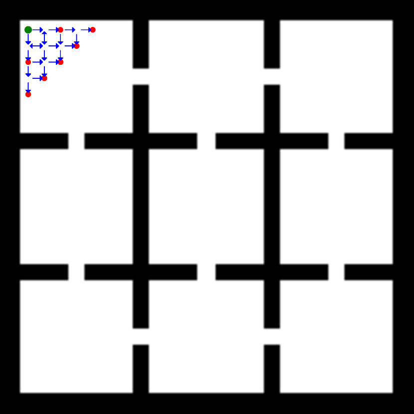
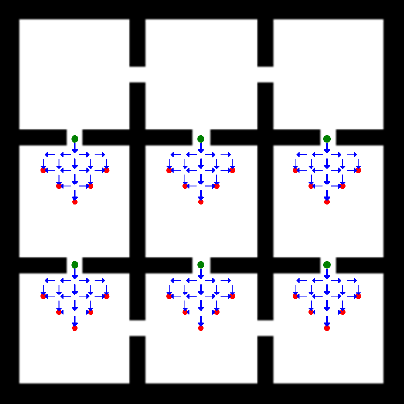
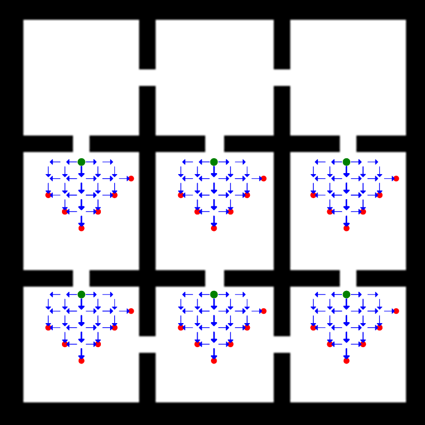
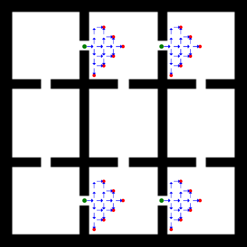
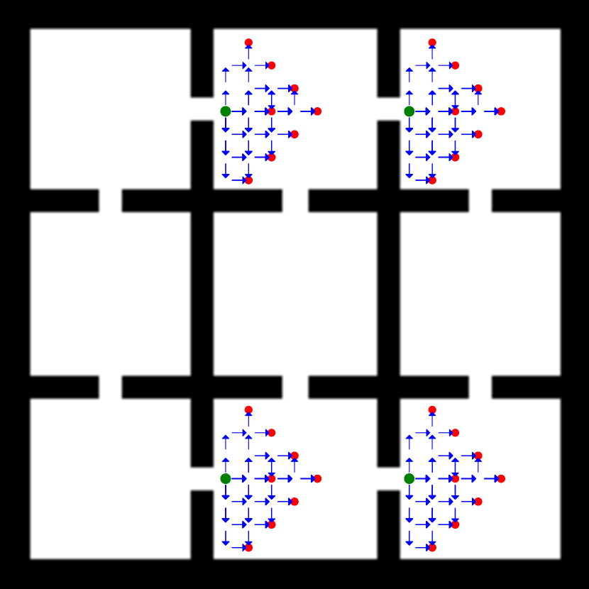
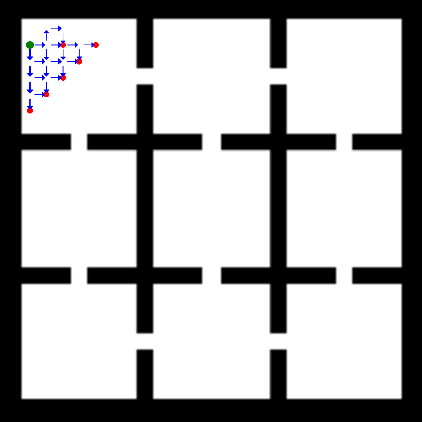
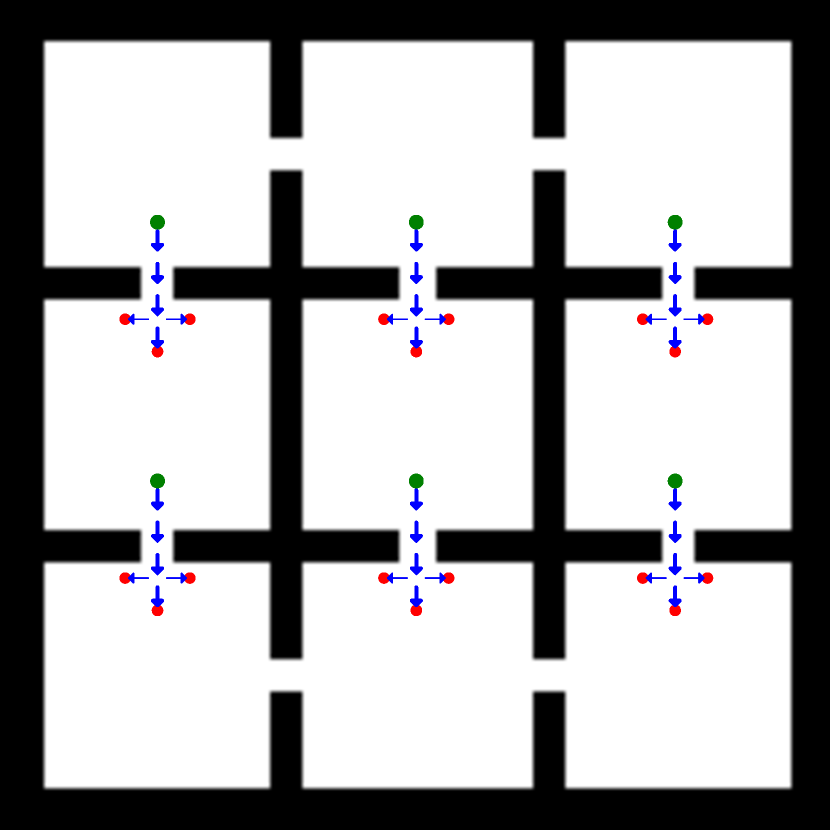
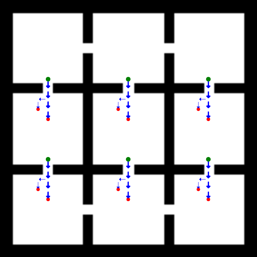
Figure 3: The eight fracture clusters with the highest expected usefulness in the Nine Rooms environment, ordered right and then down. Green points represent possible starting states, blue arrows indicate actions taken, with arrow width proportional to their frequency in the cluster, and red points denote possible termination states.

The fracture cluster in Figure 3 with the highest expected usefulness takes the agent from the starting state in all sensible directions without repetitions of movements. The majority of the other fracture clusters transverse bottlenecks, sharing the same fracture cluster where areas of local structure remain similar.

Forming multiple levels of the hierarchy. After identifying the most useful fracture clusters, they can be converted into options (as explained in Section 4.3), which extend the agent’s action space. When learning a new task, the agent can now choose from both primitive actions and these newly discovered options. The process of identifying fractures and clustering is repeated, but now the trajectories (and therefore fractures) may consist of a mix of primitive actions and higher-level options. This iterative approach naturally leads to the creation of a multi-level hierarchical structure.

4.3 Using Fracture Clusters

After selecting the most useful fracture clusters, we need to transform each cluster into an option, called a Fracture Cluster Option (FraCO). Each FraCO is characterized by an initiation set $I_{z}$, a termination condition $\beta_{z}$, and a policy $\pi_{z}$. We denote a single FraCO as $z$ and the set of all FraCOs as $Z$. Each FraCO is associated with the fracture cluster $\phi_{c}$ that forms it. We use these clusters to predict initiation states.

Initiation Set. Suppose the agent is in a state $s$, and has access to a set of actions $A$. For each state $s$, we consider possible sequences of actions of chain length $b$. Each such sequence is represented as:

$$\mathbf{a}=(a_{1},a_{2},\dots,a_{b})\mid a_{i}\in A,$$ (5)

We can now define the set of all possible fractures starting from state $s$ as,

$$F_{s}=\{(s,\mathbf{a})\mid\mathbf{a}\in A^{b}\},$$ (6)

where $A^{b}$ represents all sequences of length $b$ drawn from the action set $A$.

For each fracture $\phi=(s,\mathbf{a})$ in $F_{s}$, we estimate the likelihood that it belongs to a FraCO $z$. The set of fractures assigned to cluster $z$ in state $s$ can be defined as:

$$G_{z,s}=\{\phi\in F_{s}\mid P(\phi\in z)>\theta\},$$

where $P(\phi\in z)$ denotes the estimated probability that fracture $\phi$ belongs to cluster $z$, and $\theta$ is a threshold hyperparameter that determines cluster membership. The method for estimating $P(\phi\in z)$ can vary depending on the implementation. In our tabular implementation, we directly use the prediction function provided by HDBSCAN. In our deep implementation, a neural network predicts this probability.

A FraCO $z$ can be initiated in state $s$ if $G_{z,s}$ is not empty. Such that the initiation set is defined as,

$$I_{z}=\{s\in S\mid G_{z,s}\neq\emptyset\}.$$ (7)

Input: $G_{z,s}$, set of options $Z$, state $s$

Initialize: Select the fracture $\phi_{z}=(s,\mathbf{a})$ from $G_{z,s}$ with the highest probability $P(\phi_{z}\in z)$, where $\mathbf{a}$ is a sequence of actions $(a_{1},a_{2},\dots,a_{b})$

for each action $a_{j}$ in $\mathbf{a}$ do

       if $a_{j}$ is a primitive action then

             Execute $a_{j}$, resulting in new state $s$;

            

      else

             $a_{j}$ is another option $z^{\prime}$;

             Compute $G_{z^{\prime},s}$;

             Recursively call $\pi_{z^{\prime}}(G_{z^{\prime},s},Z,s)$;

            

       end if

      

end for

Algorithm 1 Option policy $\pi_{z}(G_{z,s},Z,s)$

Policy Execution. When FraCO $z$ is executed in state $s$, it follows the policy $\pi_{z}$, as described in Algorithm 1. The policy selects the fracture $\phi_{z}=(s,\mathbf{a})$ from $G_{z,s}$ with the highest probability $P(\phi_{z}\in z)$, and then executes the sequence of actions $\mathbf{a}=(a_{1},a_{2},\dots,a_{b})$. If one of the selected actions is another FraCO $z^{\prime}$, the agent must compute a new $G_{z^{\prime},s}$ and recursively call the policy until the option terminates.

Termination Condition. The FraCO $z$ terminates under two conditions: either when all actions in the selected fracture $\phi_{z}$ have been executed, or when no matching fracture can be found in the current state (i.e., $G_{z,s}=\emptyset$).

The termination condition $\beta(s)$ is defined as:

$$\beta(s)=\begin{cases}1&\text{if all actions in }\phi_{z}\text{ have been executed}\\ 1&\text{if }G_{z,s}=\emptyset\\ 0&\text{otherwise}\end{cases}$$ (8)

Learning with FraCOs.

In our approach, FraCOs are fixed once identified. The agent learns to choose between primitive actions and available FraCOs using standard reinforcement learning algorithms (e.g., Q-learning for tabular settings, PPO for deep learning implementations).

Example FraCO usage: An agent is in state $s$. It looks at all possible fractures in that state to form $F_{s}$. For each FraCO $z_{i}\in Z$, the agent estimates the probability $P(\phi\in z_{i})$ that each fracture $\phi\in F_{s}$ belongs to $z_{i}$. If any fractures have a probability above a threshold $\theta$, then $z_{i}$ becomes available as an option. The agent’s policy $\pi_{\text{opt}}$ selects from the available FraCOs and primitive actions. Suppose it selects FraCO $z_{1}$. The agent picks the fracture $\phi_{z_{1}}$ with the highest probability $P(\phi_{z_{1}}\in z_{1})$ and executes the sequence $\mathbf{a}$. As the agent executes these actions, if one is another FraCO, say $z_{2}$, then it forms a new $F_{s^{\prime}}$, estimates $P(\phi\in z_{2})$, and selects the most probable fracture for $z_{2}$. This process repeats until the termination condition $\beta_{z_{1}}=1$ is met, completing $z_{1}$’s execution.

5 Experimental Results

We evaluate FraCOs in three different experiments. The first focuses on OOD reward generalisation tasks using a tabular FraCOs agent in the Four Rooms, Nine Rooms, and Ramesh Maze Ramesh et al., (2019) grid-world environments (see Appendix A.7). The second examines OOD learning in state generalisation tasks within a novel environment called MetaGrid (see Appendix A.7). The final experiment evaluates a deep FraCOs agent, implemented with a three-level hierarchy using PPO in the procgen suite of environments (Cobbe et al.,, 2020). We compare its performance with CleanRL’s Procgen PPO and PPG implementations (Huang et al.,, 2022) and, Option Critic with PPO (OC-PPO) (Klissarov et al.,, 2017), see Appendices A.13 and A.13 for full method details. In the grid-world environments, the agent receives a reward of $+1$ for reaching the goal and a penalty of $-0.001$ per time step. Episodes have a maximum length of 500 steps, and a fracture chain length $b=2$. For Procgen environments, reward functions remain unchanged, and $b=3$ (see Appendix A.8 for chain-length selection details).

5.1 Experiment 1: Tabular Reward Generalisation

In this experiment, FraCOs are learned in a fixed state space $S$ while we vary the reward function $R$. The agent is allowed to discover FraCOs in 50 tasks, such that each task corresponds to a different reward location. We reserve 10 unique tasks for testing. Separate agents are trained to convergence—defined as achieving consistent performance across episodes. The top 20 FraCOs are extracted from the final trajectories of the agents, as described in Section 4, and incorporated into the action space. This extraction process is repeated four times, corresponding to each level of the hierarchy.

Four agents are created, each with an additional hierarchical level of FraCOs. After resetting their policies over options, the agents are trained on the test tasks, and evaluation episodes are conducted periodically. As shown in Figure 4, results from the Four Rooms, Nine Rooms, and Ramesh Maze environments indicate that learning is progressively accelerated on these unseen tasks as the hierarchy depth increases.

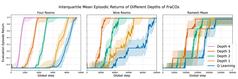
Figure 4: The interquartile mean evaluation episode rewards of a tabular FraCOs agent trained in the Four Rooms, Grid, and Ramesh Maze environments. Results are averaged over 10 independently seeded experiments, with shaded areas indicating the standard error.

5.2 Experiment 2: Tabular State Generalisation

In this experiment, we introduce a novel environment called MetaGrid, which is designed to test state and reward generalisation. MetaGrid is a navigational grid-world constructed from structured $7\times 7$ building blocks that can be combined randomly to create novel state spaces while preserving certain areas of local structure. The agent is provided with a $7\times 7$ window of observation, consistent with our other grid-worlds. For more detailed information on MetaGrid, see Appendix A.7.

At each hierarchy level, 20 FraCOs are learned from 100 randomly generated $14\times 14$ MetaGrid tasks. A task in this experiment corresponds to a differnt space space $S$ and reward location $R$. For each hierarchy level, a separate agent is created, and their policies over options are reset. These agents are then evaluated in previously unseen $14\times 14$ domains and larger $21\times 21$ domains. Periodic evaluation episodes are conducted during training to track performance, results are shown in Figure 5. These results also demonstrate an increase in the rate of learning as the hierarchy depth increases.

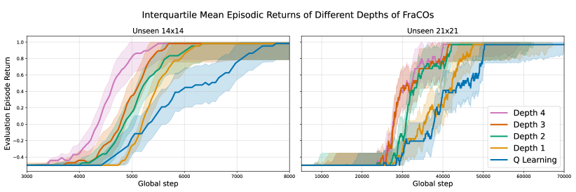
Figure 5: The interquartile mean evaluation episode rewards for tabular FraCOs in unseen MetaGrid domains of varying sizes. Results are averaged over 10 independently seeded experiments, with shaded areas indicating the standard error.

5.3 Experiment 3: Deep State and Reward Generalisation in Complex Environments

In this experiment, we test FraCOs in OOD tasks from the Procgen benchmark, focusing on unseen states spaces $S$ and reward functions $R$. We compare with three methods: Option Critic with PPO (OC-PPO) (Klissarov et al.,, 2017), a baseline PPO (Schulman et al.,, 2017), and Phasic Policy Gradient (PPG) (Cobbe et al.,, 2021) across eight Procgen environments (Cobbe et al.,, 2020). Procgen is a suite of procedurally generated arcade-style environments designed to assess generalisation across diverse tasks; see Appendix A.7 for full details.

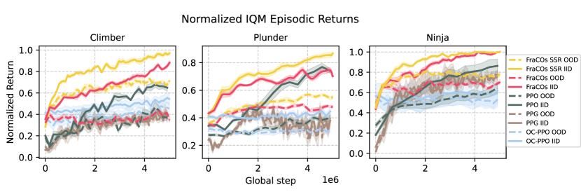
Figure 6: A comparison of learning curves of a sample of three Procgen environments.

FraCOs modifications. To handle the challenges of applying traditional clustering to high-dimensional pixel data, we simplify the approach by grouping fractures with the same action sequences, regardless of state differences. Additionally, a neural network is used to estimate initiation states and policies, which reduces the computational burden of performing a discrete search over the complex $64\times 64\times 3$ state space and managing 15 possible actions during millions of training steps. These modifications do not change the theory of FraCOs, just the implementation. Full details of these modifications are provided in Appendix A.10, with further information on the experiments, baselines, and hyperparameters in Appendix A.11.

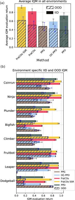
Figure 7: Final min-max normalised IQM returns with standard errors across Procgen environments.

FraCOs and OC-PPO both learn options during a 20-million time-step warm-up phase, with tasks drawn from the first 100 levels of each Procgen environment. FraCOs learns two sets of 25 options, corresponding to different hierarchy levels, while OC-PPO learns a total of 25 options. After the warm-up, the policy over options is reset, and training continues for an additional 5 million time steps. During this phase, we periodically conduct evaluation episodes on both IID and OOD tasks, with OOD tasks drawn from Procgen levels beyond 100.

We test two versions of FraCOs: one where the policy over options is completely reinitialized after the warm-up phase, and another that transfers a Shared State Representation (SSR), referred to as FraCOs-SSR. In the SSR, a shared convolutional layer encodes the state, followed by distinct linear layers for the critic, policy over options, and option policies. These convolutional layers are not reset after warm-up, enabling a shared feature representation across tasks. Since OC-PPO inherently relies on a shared state representation to define its options and meta-policy, comparing it with FraCOs-SSR offers a fairer evaluation. Without this shared representation, OC-PPO struggles to maintain stable and meaningful options across tasks. Despite this adjustment for fairness, we find that FraCOs, even without SSR, consistently outperforms both baselines. For further implementation details of FraCOs-SSR, see Appendix A.11.

Figure 7 (a) provides the min-max normalised interquartile mean (IQM) across all Procgen environments. Figure 7 (b) provides the results of each environment. We also provide three example learning curves in Figure 6. Each experiment was repeated with eight seeds. On average we observe that FraCOs and FraCOs-SSR are able to improve both IID and OOD returns over all baselines.

6 Discussion and Limitations

This study introduced Fracture Cluster Options (FraCOs) as a novel framework for multi-level hierarchical reinforcement learning. In tabular settings, FraCOs demonstrated accelerated learning on unseen tasks, with performance improving as hierarchical depth increased. In deep RL experiments, FraCOs outperformed OC-PPO, PPO, and PPG on both in-distribution (IID) and out-of-distribution (OOD) tasks, showcasing its potential for robust generalization. While PPG maintained a smaller generalization gap (the difference between IID and OOD performance), integrating FraCOs with a PPG baseline could achieve both higher performance and reduced generalisation gaps. Error bars

However, FraCOs faces limitations. Clustering methods struggle with prediction accuracy as environments grow more complex, and while simplified techniques and neural networks were introduced, further research into scalable clustering solutions is needed. Additionally, this work focused on discrete action spaces; extending FraCOs to continuous action spaces remains as future work.

Despite these limitations, FraCOs provides a strong foundation for advancing hierarchical reinforcement learning and improving generalisation across tasks.

Appendix A Appendix

A.1 Glossary

Glossary of Terms and Derivations

Term/Symbol	Definition/Derivation
MDP (Markov Decision Process)	A mathematical framework for modeling decision-making, defined by the tuple $\langle S,A,P,R,\gamma\rangle$, where: • $S$: Set of possible states. • $A$: Set of possible actions. • $P$: Transition probability function, $P(s,a,s^{\prime})$. • $R$: Reward function, $R(s,a,s^{\prime})$. • $\gamma$: Discount factor, $\gamma\in[0,1]$.
$S$	Set of possible states in an MDP.
$A$	Set of possible actions in an MDP.
$P$	Transition probability function; $P(s,a,s^{\prime})$ gives the probability of transitioning from state $s$ to $s^{\prime}$ after action $a$.
$R$	Reward function; $R(s,a,s^{\prime})$ is the reward received when transitioning from $s$ to $s^{\prime}$ via action $a$.
$\gamma$	Discount factor in an MDP, $\gamma\in[0,1]$, representing the importance of future rewards.
$s_{t}$	State of the agent at time step $t$.
$a_{t}$	Action taken by the agent at time step $t$.
$s^{\prime}$	Next state after taking action $a_{t}$ from state $s_{t}$.
$\pi(s_{t})$	Policy of the agent, mapping state $s_{t}$ to a probability distribution over actions.
$G_{t}$	Cumulative discounted return from time $t$, defined as $G_{t}=\sum_{k=0}^{\infty}\gamma^{k}r_{t+k+1}$.
Trajectory ($\tau\in T$ )	A sequence of states, actions, and rewards experienced by the agent: $\tau=(s_{0},a_{0},r_{1},s_{1},a_{1},r_{2},\dots)$.
Task	A task is defined as a unique MDP.
Reward generalisation tasks	MDPs with $R$ values outside of the training distribution, while $S$, $A$, $P$, and $\gamma$ remain within distribution.
State generalisation tasks	MDPs with $S$ and $R$ values outside of the training distribution, while $A$, $P$, and $\gamma$ remain within distribution.
Option	In HRL, a temporally extended action, defined by: • $I$: Initiation set. • $\pi_{\text{intra}}$: Intra-option policy. • $\beta(s)$: Termination condition.
$I$	Initiation set of an option; the set of states where the option can be initiated.
$\pi_{\text{intra}}$	Intra-option policy; the policy followed while the option is active.
$\beta(s)$	Termination condition of an option; gives the probability of terminating the option in state $s$.
FraCOs (Fracture Cluster Options)	The proposed method for defining, forming, and utilizing multi-level hierarchical options based on expected future usefulness.
$\phi$	A fracture; a state paired with a sequence of actions: $$\phi=(s_{t},a_{t},a_{t+1},\dots,a_{t+b-1})$$
$b$	Chain length of a fracture; specifies the number of actions following the state $s_{t}$.
$F$	Set of fractures derived from a single trajectory: $$F=\{(s_{t},a_{t},a_{t+1},\dots,a_{t+b-1})\mid 0\leq t\leq n-b\}$$
$\Phi$	Complete set of fractures from all trajectories: $$\Phi=\{F_{1},F_{2},\dots,F_{|\mathcal{T}|}\}$$
$\phi_{c}$	A fracture cluster; a group of fractures with similar behaviors.
Usefulness Metric ($U(\phi_{c})$)	A measure to evaluate fracture clusters based on their potential for reuse in future tasks: $$U_{(\phi_{c})}=\frac{1}{3}\left(P[\phi_{c}\in\tau_{s}\mid x_{s}]+P[\phi_{c}\mid\Phi_{s}]+H(\phi_{c}\mid\mathcal{X}_{s})\right)$$
Expected Usefulness terms	• $\omega_{n}$: Appearance indicator; $\omega_{n}=1$ if any fracture $\phi\in\phi_{c}$ appears in trajectory $\tau_{n}$, else $0$. • $\alpha$, $\beta$: Parameters of the Beta prior distribution, typically set to $1$. • $N$: Total number of experienced tasks. • $\Phi_{s}$: Set of all successful fractures. • $T_{s}$: Set of successful trajectories. • $N_{\phi_{c}}$: Normalization constant for entropy calculation.
Derivation of Appearance Probability	Using Bayesian inference, the appearance probability is estimated as: $$P[\phi_{c}\in\tau_{s}\mid x_{s}]=\frac{\sum_{n=1}^{N}\omega_{n}+\alpha}{N+\alpha+\beta}$$ (9) Where $\omega_{n}$ are observations modeled as Bernoulli random variables with a Beta prior.
Derivation of Relative Frequency	Calculated as: $$P[\phi_{c}\mid\Phi_{s}]=\frac{\text{count}(\phi_{c},\Phi_{s})}{|\Phi_{s}|}$$ (10) Where $\text{count}(\phi_{c},\Phi_{s})$ is the number of times fractures in $\phi_{c}$ appear among all successful fractures $\Phi_{s}$.
Derivation of Entropy of Usage	The entropy of a fracture cluster’s usage is: $$H(\phi_{c}\mid\mathcal{X}_{s})=-\sum_{\tau_{s}\in T_{s}}\frac{\text{count}(\phi_{c},\tau_{s})}{|\tau_{s}|}\log_{N_{\phi_{c}}}\left(\frac{\text{count}(\phi_{c},\tau_{s})}{|\tau_{s}|}\right)$$ (11) This measures the diversity of the fracture cluster’s usage across tasks.
$\alpha,\beta$	Parameters of the Beta distribution used in Bayesian estimation; set to $\alpha=1$, $\beta=1$ for an uninformative prior.
$\omega_{n}$	Appearance indicator for task $n$; $\omega_{n}=1$ if any fracture in $\phi_{c}$ appears in trajectory $\tau_{n}$, else $0$.
$Z$	Set of all Fracture Cluster Options (FraCOs).
$z$	A single FraCO; an option derived from a fracture cluster.
$I_{z}$	Initiation set of FraCO $z$; states where $z$ can be initiated: $$I_{z}=\{s\in S\mid G_{z,s}\neq\emptyset\}$$
$\beta_{z}$	Termination condition of FraCO $z$; $z$ terminates when all actions in the selected fracture have been executed or when no matching fracture is found: $$\beta(s)=\begin{cases}1&\text{if all actions in }\phi_{z}\text{ have been executed}\\ 1&\text{if }G_{z,s}=\emptyset\\ 0&\text{otherwise}\end{cases}$$
$\pi_{z}$	Policy of FraCO $z$; defines the sequence of actions when the option is active (see Algorithm 1 in the paper).
$G_{z,s}$	Set of fractures assigned to cluster $z$ in state $s$: $$G_{z,s}=\{\phi\in F_{s}\mid P(\phi\in z)>\theta\}$$
$\theta$	Threshold hyperparameter for cluster membership; determines if a fracture belongs to a cluster based on probability.
$N$	Total number of experienced tasks or samples.
$\mathcal{T}$	Set of all trajectories.
$\tau$	An individual trajectory from the set $\mathcal{T}$.
$\tau_{s}$	A successful trajectory; meets a predefined success criterion.
$T_{s}$	Set of successful trajectories.
$\mathcal{X}_{s}$	Set of tasks corresponding to successful trajectories.
$A$	Action set of the environment; may include primitive actions and options.
$N_{c}$	Number of cluster-options (options derived from fracture clusters).

A.2 Derivation of Usefulness Metric

In this appendix, we derive the usefulness ($U$) metric for fracture clusters. This metric is used to identify which fracture clusters have the greatest potential for reuse across different tasks. Usefulness is a function of the following three factors:

1. The probability that a fracture cluster appears in any given successful task:

   $$P[\phi_{c}\in\tau_{s}|x_{s}]$$

2. The probability that a fracture cluster is selected from the set of successful fracture clusters:

   $$P[\phi_{c}|\Phi_{s}]$$

3. The entropy of the fracture cluster’s usage across all successful tasks:

   $$H(\phi_{c}\mid\mathcal{T}_{s})$$

Usefulness ($U$) is then defined as the normalized sum of these three factors:

$$U=\frac{1}{3}\left(P[\phi_{c}\in\tau_{s}|x_{s}]+P[\phi_{c}|\Phi_{s}]+H(\phi_{c}\mid\mathcal{T}_{s})\right)$$

The objective is to select fracture clusters that maximize the usefulness, i.e.,

$$\arg\max_{\phi_{c}}U(\phi_{c})$$

A.3 Deriving $P[\phi_{c}\in\tau_{s}|x_{s}]$ Using Bayesian Inference

We want to model the probability that a fracture cluster $\phi_{c}$ appears in any given successful task, $P[\phi_{c}\in\tau_{s}|x_{s}]$. For each successful task $x_{s}$ from the set of successful tasks $\mathcal{X}_{s}$, the presence of fracture cluster $\phi_{c}$ in the corresponding trajectory $\tau_{s}$ is represented by a binary random variable $\omega_{s}$, where:

$$\omega_{s}=\begin{cases}1&\text{if}\,\phi_{c}\in\tau_{s}\,(\text{fracture cluster appears in the trajectory}),\\ 0&\text{otherwise}\end{cases}$$

The variable $\omega_{s}$ is modeled as a Bernoulli random variable:

$$\omega_{s}\sim\text{Bernoulli}(p)$$

where $p$ is the probability that fracture cluster $\phi_{c}$ appears in the trajectory $\tau_{s}$ of task $x_{s}$.

Since we are uncertain about the true value of $p$, we place a Beta distribution prior on $p$:

$$p\sim\text{Beta}(\alpha,\beta)$$

where $\alpha$ and $\beta$ are hyperparameters representing our prior belief about the likelihood of $\phi_{c}$ appearing in a trajectory.

Given a total of $N$ tasks, the likelihood for each observation $\omega_{s}$ is:

$$P(\omega_{n}|p)=p^{\omega_{n}}(1-p)^{1-\omega_{n}}$$

where $\omega_{n}$ is 1 if $\phi_{c}$ appears in trajectory $\tau_{s}$ for task $x_{n}$, and 0 otherwise.

Using Bayes’ theorem, the posterior distribution of $p$ after observing data is:

$$P(p|\omega_{1},\dots,\omega_{N})\propto P(\omega_{1},\dots,\omega_{N}|p)P(p)$$

Substituting the likelihood and the Beta prior, we get:

$$P(p|\omega_{1},\dots,\omega_{N})\propto\prod_{n=1}^{N}p^{\omega_{n}}(1-p)^{1-\omega_{n}}\cdot p^{\alpha-1}(1-p)^{\beta-1}$$

This simplifies to:

$$P(p|\omega_{1},\dots,\omega_{N})\propto p^{\sum_{n=1}^{N}\omega_{n}+\alpha-1}(1-p)^{N-\sum_{n=1}^{N}\omega_{n}+\beta-1}$$

Thus, the posterior distribution for $p$ follows a Beta distribution:

$$p|\omega_{1},\dots,\omega_{N}\sim\text{Beta}(\alpha_{N},\beta_{N})$$

where:

$$\alpha_{N}=\sum_{n=1}^{N}\omega_{n}+\alpha,\quad\beta_{N}=N-\sum_{n=1}^{N}\omega_{n}+\beta$$

In our experiments, we set $\alpha=1$ and $\beta=1$, representing an uninformative prior.

A.4 Deriving $P[\phi_{c}|\Phi_{s}]$

The second component of the usefulness metric, $P[\phi_{c}|\Phi_{s}]$, is the probability that fracture cluster $\phi_{c}$ is selected from the set of successful fracture clusters. This can be computed as the relative frequency of $\phi_{c}$ in the set $\Phi_{s}$ of successful clusters:

$$P[\phi_{c}|\Phi_{s}]=\frac{\text{count}(\phi_{c},\Phi_{s})}{|\Phi_{s}|}$$

where $\text{count}(\phi_{c},\Phi_{s})$ is the number of times $\phi_{c}$ appears in the set of successful clusters, and $|\Phi_{s}|$ is the total number of successful clusters.

A.5 Deriving $H(\phi_{c}\mid\mathcal{T}_{s})$

The entropy term $H(\phi_{c}\mid\mathcal{T}_{s})$ measures the unpredictability or diversity of the usage of fracture cluster $\phi_{c}$ across successful tasks. Entropy is defined as:

$$H(\phi_{c}\mid\mathcal{T}_{s})=-\sum_{\tau_{s}\in\mathcal{T}_{s}}p[\phi_{c}\mid\tau_{s}]\cdot\log_{N_{\phi_{c}}}(p[\phi_{c}\mid\tau_{s}])$$

where $p[\phi_{c}\mid\tau_{s}]$ is the proportion of times that fracture cluster $\phi_{c}$ appears in trajectory $\tau_{s}$:

$$p[\phi_{c}\mid\tau_{s}]=\frac{\text{count}(\phi_{c},\tau_{s})}{|\tau_{s}|}$$

Here, $|\tau_{s}|$ represents the length of the trajectory $\tau_{s}$, and $N_{\phi_{c}}$ is the total number of fracture clusters considered. The choice of logarithm base, $N_{\phi_{c}}$, reflects the fact that we normalize entropy relative to the number of fracture clusters.

A.6 Expected Usefulness

Having derived the empirical estimations of the three components of usefulness we can now combine these elements to calculate the expected usefulness of each fracture cluster. The expected usefulness incorporates the posterior distribution from Bayesian inference for $P[\phi_{c}\in\tau_{s}|x_{s}]$, as well as the empirical counts for the other components.

Thus, the expected usefulness for each fracture cluster is calculated as:

$$E[U(\phi_{c})]=\frac{1}{3}\left(\frac{\sum_{n=1}^{N}\omega_{n}+\alpha}{N+\alpha+\beta}+\frac{\text{count}(\phi_{c},\Phi_{s})}{|\Phi_{s}|}-\sum_{\tau_{s}\in\mathcal{T}_{s}}\frac{\text{count}(\phi_{c},\tau_{s})}{|\tau_{s}|}\cdot\log_{N_{\phi_{c}}}\left(\frac{\text{count}(\phi_{c},\tau_{s})}{|\tau_{s}|}\right)\right)$$

where $\alpha$ and $\beta$ are the parameters of the beta distribution, which we set to $\alpha=1$ and $\beta=1$ in our experiments.

By calculating this expected usefulness, we can rank the fracture clusters according to their potential for reuse in future tasks. The ranking helps focus on fracture clusters that are more likely to appear in successful outcomes and contribute to the agent’s performance across diverse scenarios.

A.7 Environments

This section provides details on the environments used in our experiments, including standard grid-world domains (Four Rooms, Grid, Ramesh Maze), MetaGrid, and the Procgen suite. Each environment has been designed to evaluate different aspects of the agent’s behaviour, such as navigation, exploration, and task performance.

A.7.1 Grid-World Environments

We use three standard grid-world environments: Four Rooms, Grid, and Ramesh Maze. Figure 8 illustrates these environments.

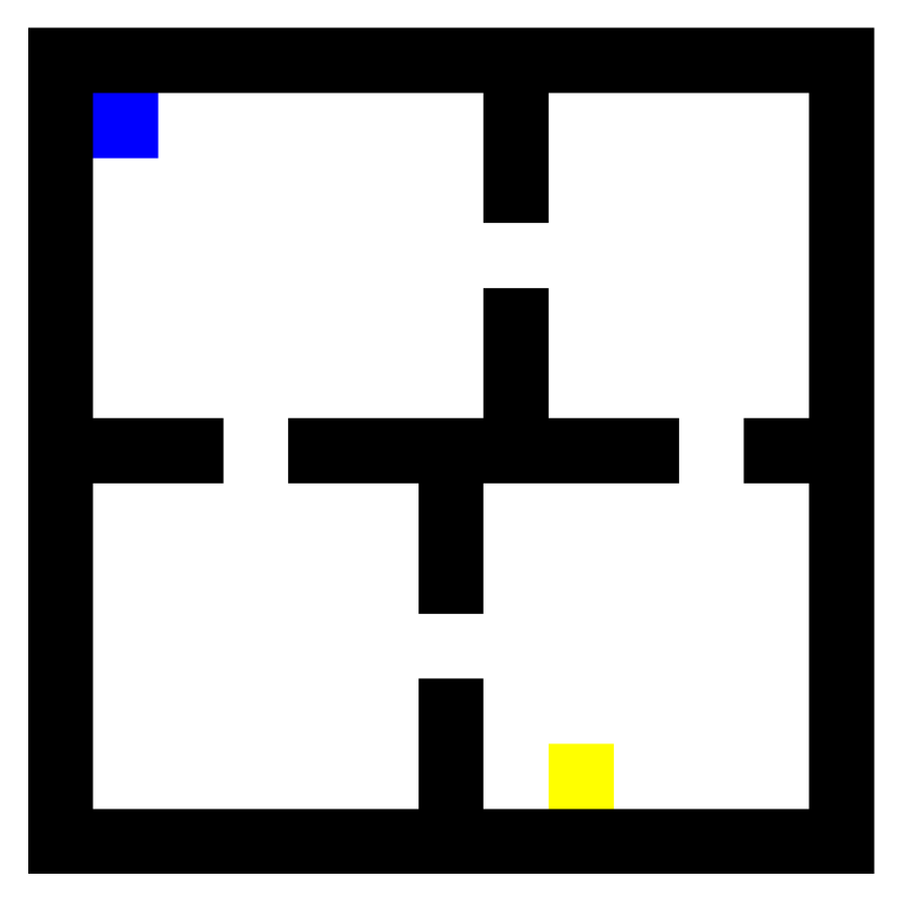
(a) Four rooms

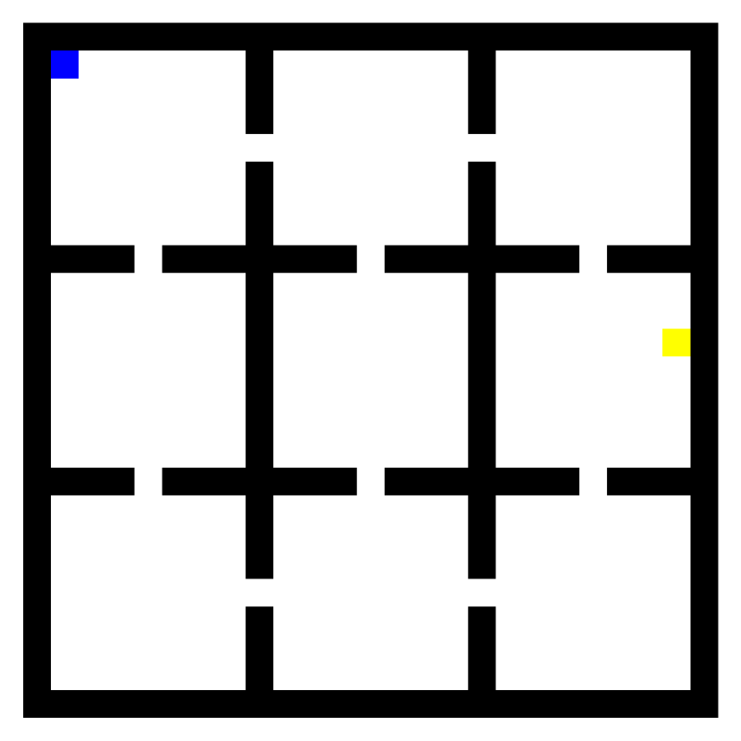
(b) Grid

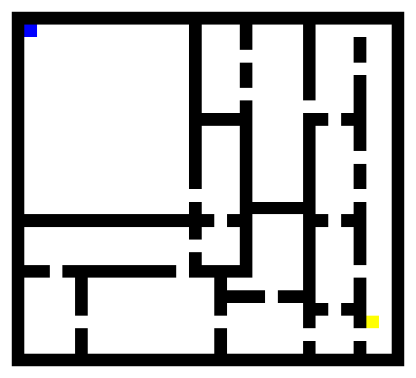
(c) Ramesh maze

Figure 8: Examples of the Four Rooms (a), Grid (b), and Ramesh Maze (c) environments. In each, black represents walls, blue represents the agent, yellow represents the goal, and white represents empty space. The agent can move up, down, left, and right, receiving a reward upon reaching the goal. The goal’s location in these figures is an example of one of many possible positions. These versions of Four Rooms, Grid and Ramesh Maze are part of the MetaGrid suite and thus have a 7x7 observation space centered on the agent.

In these grid-world environments, the action space is discrete, with four possible (primitive) actions:

$$A=\{0,1,2,3\}$$

These actions correspond to moving Up, Down, Left, and Right, respectively. The agent’s observation space is a 7x7 grid centered on itself, meaning it only observes a portion of the environment at any given time. This localized view allows the agent to learn how to navigate based on nearby features. This design is similar to MiniGrid (Chevalier-Boisvert et al.,, 2023), but in our case, the observations are ego-centric, always centered on the agent.

In tabular learning, the agent uses this 7x7 observation space to predict initiation states, though the Q-function is still based on absolute coordinates. We do not employ state-transition graphs in any of our experiments.

A.7.2 MetaGrid Environment

The MetaGrid environment extends the standard grid-world setup by allowing for procedurally generated maps of varying sizes. MetaGrid introduces randomness in the layout of walls and goal locations, ensuring that the agent encounters a diverse set of environments during training and evaluation. Figure 9 demonstrates the building blocks which all environments in MetaGrid are formed from, and Figure 10 shows examples of MetaGrid environments in two different sizes: 14x14 and 21x21.

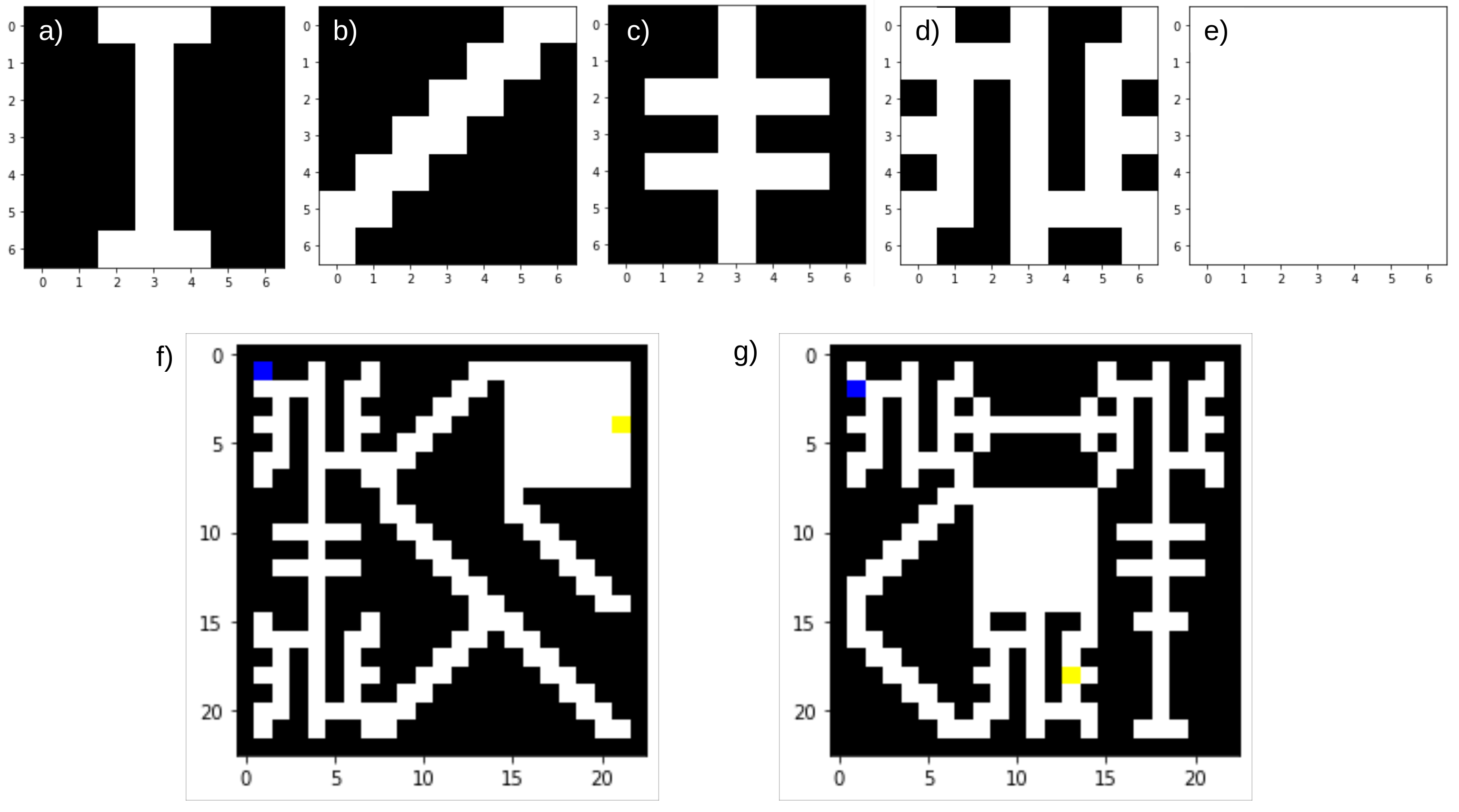
Figure 9: a) - e) demonstrate the building blocks which MetaGrid domains can be created from. f) and g) demonstrate two 21x21 configurations using these building blocks.

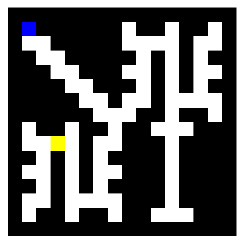
(a)

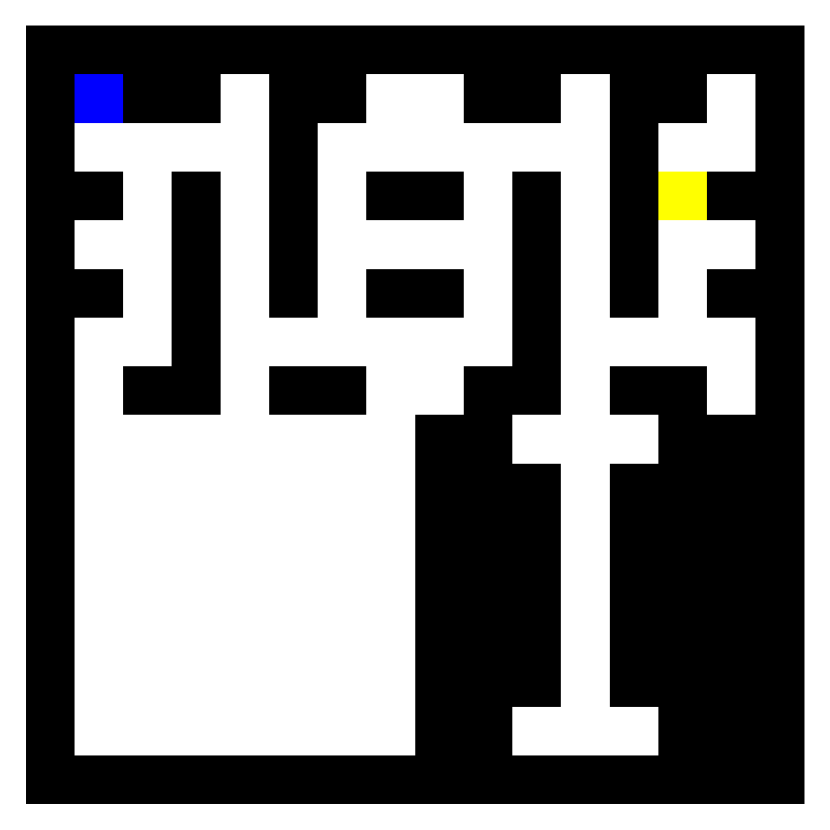
(b)

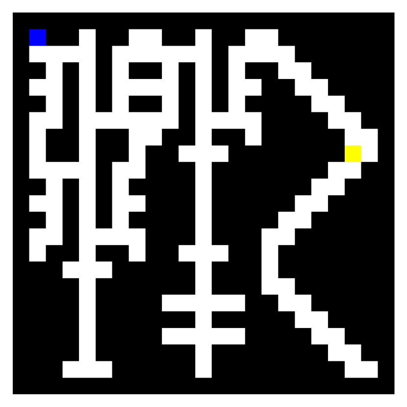
(c)

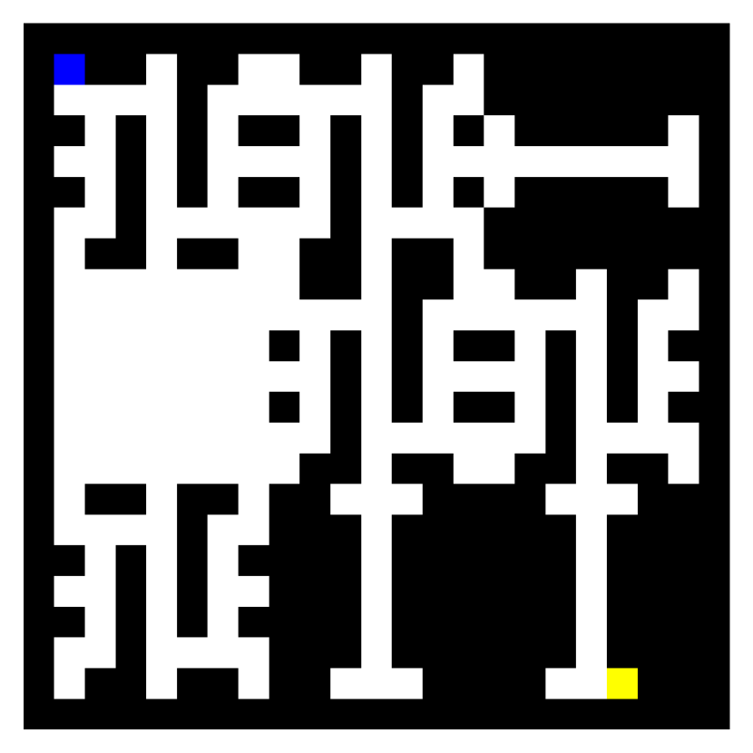
(d)

Figure 10: Examples of randomly generated MetaGrid environments. The blue square represents the agent, yellow represents the reward, white represents empty space, and black represents walls. Subfigures (a) and (b) show 14x14 grids, while (c) and (d) show 21x21 grids.

The action space in MetaGrid is identical to the one used in the standard grid worlds, with four discrete actions: Up, Down, Left, and Right. Similarly, the agent observes a 7x7 grid centered on itself, allowing it to make decisions based on local information. The procedural generation in MetaGrid provides varied environments for the agent to adapt to, making it a more challenging and dynamic environment compared to static grid worlds.

A.7.3 Procgen Environments

Procgen is a suite of procedurally generated environments designed to test generalisation and performance across diverse tasks such as navigation, exploration, combat, and puzzle-solving. Each environment provides a different variation on every reset, preventing the agent from memorizing specific layouts or solutions. Please see Cobbe et al., (2020) for the full details of these environments.

Action Space Procgen environments feature discrete actions like movement (up, down, left, right) and interactions (e.g., jump, shoot). Depending on the task, the action space can range from 5 to 15 actions, covering basic navigation and task-specific interactions.

Observation Space Unlike grid-based environments, Procgen uses 64x64 RGB pixel observations, providing rich visual input. The agent must interpret features such as walls, enemies, and obstacles to navigate and interact effectively.

Rewards Rewards in Procgen are sparse, given for completing tasks like reaching goals or defeating enemies. The agent must learn to explore efficiently and develop strategies for long-term success.

Optional Parameters To simplify learning and reduce computational cost, we activated the following Procgen parameters:

• Distribution mode = “easy": Provides easier levels.

• Use backgrounds = “False": Backgrounds are black to avoid additional noise.

• Restrict themes = “True": Limits visual variation to a single theme, such as consistent wall styles in environments like CoinRun.

Overall, these environments—ranging from grid-world environments with discrete action spaces and ego-centric observations to the more complex Procgen environments with pixel-based observations—offer a diverse set of challenges for our agents. The combination of procedurally generated environments in MetaGrid and Procgen ensures that the agents are tested on both fixed and highly variable environments, making them suitable for evaluating the robustness of the learning algorithms used in our experiments.

A.7.4 UMAP visualisations of other environments

The structure observed in the latent projections of clustered Fracos as seen in Section 4.1 is also demonstrated in trained agents of other simple environments; Figure 11 visualises fracture structures in Grid (Nine rooms), CartPole, and LunarLander. The Grid environment is shown in Figure 8, CartPole and LunarLander are standard environments from the Farama Foundation Gymnasium suite Towers et al., (2023).

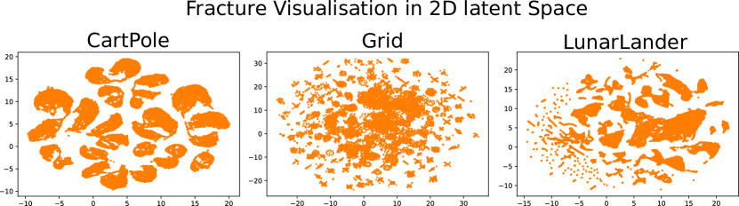
Figure 11: Two dimensional visualisations of the fractures formed for trained agents in CartPole, Grid (Nine Rooms) and LunarLander .

A.8 FraCOs Chain Lengths and Depth Limits

In our FraCOs method, the process of matching clusters involves conducting a discrete search over potential action permutations. This process requires forming all possible permutations of actions and passing them through the saved clusterer to determine which permutation is currently viable for the meta-policy to choose. The complexity of this search is captured by the permutation formula:

$${}^{B}P_{N_{c}}=\frac{N_{c}!}{(N_{c}-B)!}$$

where $B$ is the length of the action chain, and $N_{c}$ is the total number of cluster-options. As a result, the time complexity for performing this search grows factorially, $O\left(\frac{N_{c}!}{(N_{c}-B)!}\right)$, as more cluster-options are introduced or when the chain length is increased. This rapidly becomes computationally expensive as these numbers increase.

A.8.1 Chain Length and Depth in Tabular Experiments

Due to this factorial growth, it is crucial to limit the number of cluster-options and the chain length in experiments that involve discrete cluster search (Experiments 1, 2 and 3.1). For all experiments using cluster search, we chose a chain length of 2 to keep the computational complexity manageable. Additionally, we restricted the depth of the FraCOs hierarchy to 3 or 4 levels, depending on the complexity of the environment.

This limitation on depth and chain length helps maintain a balance between the richness of the learned options and the feasibility of performing the cluster search in a reasonable amount of time. The factorial growth of the search process becomes prohibitive as more cluster-options or deeper chains are introduced, making this constraint necessary for efficient execution of our experiments.

A.8.2 Why This Isn’t a Problem for Neural Network Cluster Predictions

In contrast, when we extend the FraCOs initiation and action estimation to be used with neural networks, the limitation of conducting computationally expensive permutation searches is alleviated. Neural networks can learn initiation sets and make predictions in a continuous manner, bypassing the need for discrete cluster searches. This removes the necessity of factorially growing search complexity, allowing for more flexibility in chain lengths and depth.

However, the challenge in neural network experiments lies in the sheer number of timesteps required for training and evaluation. For example, in our deep experiments (at a depth of two), training involved many millions of timesteps across nine different environments, totaling 180 million steps for pre-training, repeated for three seeds. Testing required an additional 120 million steps, also repeated for three seeds. This was only for FraCOs. When we include experiments using OC (Option Critic), PPO, and PPO25, the total number of timesteps across all experiments becomes 3.06 billion.

To manage these computational demands, we used a chain length of 3. This allowed us to conduct only two warm-up phases, while ensuring that options could still be executed for a reasonable duration (a maximum of nine steps, i.e., 3x3). This setup enabled us to complete the necessary pre-training and testing without sacrificing the quality of the learned options while maintaining computational feasibility.

A.9 FraCOs Experiment Parameters for Tabular Methods

Tabular Q-Learning is a reinforcement learning algorithm where the agent learns the optimal action-value function $Q(s,a)$, which estimates the expected cumulative reward for taking action $a$ in state $s$ and following the optimal policy thereafter. The agent interacts with the environment, updates the Q-values for each state-action pair based on rewards, and converges to the optimal policy over time Sutton and Barto, (2018). We implement a vectorized Q learning method.

The key hyperparameters used in all Tabular Q-Learning experiments are listed in Table 2.

Table 2: Hyperparameters for Tabular Q-Learning Experiment

Hyperparameter	Value	Description
eps	0.1	Exploration rate for $\epsilon$-greedy policy. Determines the probability of taking a random action instead of the action with the highest Q-value.
alpha	0.1	Learning rate for Q-value updates. Controls how much the Q-value is updated in each iteration.
gamma	0.99	Discount factor for future rewards.
num_steps	64	Number of steps per episode before environment reset.
max_ep_length	1000	Maximum timesteps allowed in an episode.
anneal_lr	True	Whether to anneal the learning rate as training progresses.
batch_size	64	Number of state-action-reward tuples processed in a batch.
Number of Envs	64	Number of vectorized environments

In Tabular Q-Learning, the agent repeatedly updates its Q-values for each state-action pair, gradually converging to the optimal policy. By balancing exploration and exploitation, adjusting the learning rate, and prioritizing long-term rewards, the agent learns to optimize its decision-making in the given environment.

FraCOs (Fracture Cluster Options) for Tabular Methods: For reproducibility, the key hyperparameters used in the clustering process and other implementation details are outlined below.

In all tabular experiments, we use HDBSCAN as the clustering method (Campello et al.,, 2013). The clustering hyperparameters are:

Table 3: Clustering Hyperparameters for FraCOs

Hyperparameter	Value
Chain length (b)	2
Minimum cluster size	15
Metric	Euclidean
Minimum samples	1
Generate minimum spanning tree	True

The following table lists the minimum success rewards required for each environment:

Table 4: Minimum Success Reward per Environment

Environment	Minimum Success Reward
Four Rooms	0.97
Grid	0.60
Ramesh Maze	0.70
MetaGrid 14x14	0.95

FraCOs-Specific Hyperparameters:

Table 5: FraCOs Hyperparameters

Hyperparameter	Value
Generalisation strength	0.01
FraCOs bias factor	100
FraCOs bias depth anneal	True

The generalisation strength represents the threshold a fracture cluster must pass to be considered for initiation. The threshold is defined as $1-\texttt{HDBSCAN.predict.strength}>$ generalisation strength.

The FraCOs bias factor determines how much initial Q-values should be scaled to encourage transfer, similar to optimistic initial values. For FraCOs bias depth annealing, the bias depth increases with deeper FraCOs. For example, with a bias factor of 100 and depth of 3, the first bias is scaled by the cube root of 100, the second by the square root, and the final by 100.

A.10 FraCOs Modifications for Deep Learning

In our experiments with deep learning, particularly in environments with large state spaces such as the 64x64x3-dimensional Procgen environments, we found that HDBSCAN failed to accurately capture meaningful clusters or predict clusters effectively. Initially, we attempted to integrate a Variational Autoencoder (VAE) to use its latent space representation in the fracture formation process Kingma and Welling, (2013). However, clustering methods still struggled to deliver satisfactory results.

Consequently, we adopted a simpler clustering approach and shifted to using neural networks to predict both the initiation states and the policy.

Simpler Clustering. To simplify the clustering process, we based clusters solely on sequences of actions. For instance, with a chain length of three, any fracture formed by the action sequence “up", “up", “right" was clustered together, independent of the state. While this approach overlooks some intricacies captured by state-based fracture formations, it was necessary to handle the increased complexity of environments like Procgen.

Cluster Selection. The cluster selection process remained unchanged. We continued to use the usefulness metric, as defined in Equation 4, to select clusters.

Initiation Prediction. Instead of relying on clustering methods to predict initiation states, we trained a neural network to predict the states corresponding to each fracture cluster. This process involved two steps:

1. First, we trained a Generative Adversarial Network (GAN) to augment the states in each fracture cluster (since neural networks typically require large datasets).

2. Using both the real and generated states, we trained a neural network as a classifier to predict which fracture cluster a given state belonged to. One neural network was trained to predict all initiations at each hierarchical level. This method significantly improved efficiency, reducing the need for permutation-based discrete searches to a single forward pass.

Policy Prediction. For policy prediction, we utilized a shortcut. Since all FraCOs are derived from trajectories generated by a pre-trained agent, the policy of this trained agent already serves as an approximation for the FraCO policy. We saved the agent’s policy at the end of trajectory generation and used it as the policy for all FraCOs. This reuse of the agent’s policy minimized additional computation without sacrificing accuracy.

Termination Condition. The termination condition for each FraCO was determined solely by the chain length, maintaining a fixed execution limit per option.

A.11 Experiment Parameters for Deep Methods

All deep methods in our experiments were based on CleanRL’s implementation of PPO for the Procgen environments, and we used the same hyperparameters from this implementation. This ensured that the PPO baseline was hyperparameter-tuned, providing a strong and well-optimized baseline for comparison. However, FraCOs and OC-PPO were not specifically hyperparameter-tuned for these environments. Despite this, we consider it reasonable to assume that FraCOs and OC-PPO would perform near their best, as they share similar PPO update mechanisms and underlying structures with the baseline PPO.

While there exists an implementation of OC-PPO by Klissarov et al., (2017), we opted to implement our own version to maintain consistency with CleanRL’s PPO implementation. This approach was necessary to ensure that any observed differences in performance were due to algorithmic design rather than implementation differences.

We chose OC-PPO over the standard Option Critic for two primary reasons. First, in our experiments with the standard Option Critic, we observed that the options collapsed quickly, converging to the same behaviour. By integrating the entropy bonus provided by the PPO update, we were able to alleviate this collapse and maintain more diverse option behaviours. Second, PPO has demonstrated significantly better performance than Advantage Actor Critic (A2C) (Mnih,, 2016) in the Procgen environments. Given that the original Option Critic framework is based on A2C, using it as a baseline would have led to an unfair comparison, as A2C has been shown to be less effective in these environments. Therefore, incorporating PPO in both FraCOs and OC-PPO allowed for a fairer and more balanced comparison.

We outline the hyperparameters which we used in the implementation below. All code will be provided from the authors github upon publication.

A.11.1 PPO

We use CleanRL’s Procgen implementation as our baseline Huang et al., (2022). The only adaption we make is that we implement entropy annealing, we also have some wrappers which mean Procgen can be used with the Gymnasium API. We have another wrapper which is used for handling multi-level FraCOs in vectorized environments. These wrappers are also applied to the baseline PPO.

Hyperparameters Table 6 provide hyperparameters for PPO.

Parameter	Value	Explanation
easy	1	1 activates “easy" Procgen setting
gamma	0.999	The discount factor.
vf_coef	0.5	Coefficient for the value function loss.
ent_coef	0.01	Entropy coefficient.
norm_adv	true	Whether to normalize advantages.
num_envs	64	Number of parallel environments.
anneal_lr	true	Whether to linearly anneal the learning rate.
clip_coef	0.1	Clipping coefficient for the policy objective in PPO.
num_steps	256	Number of decisions per environment per update.
anneal_ent	false	Whether to anneal the entropy coefficient over time.
clip_vloss	true	Whether to clip the value loss in PPO.
gae_lambda	0.95	The lambda parameter for Generalized Advantage Estimation (GAE).
proc_start	1	Indicates the starting level for Procgen environments.
learning_rate	0.0005	The learning rate for the PPO optimizer.
max_grad_norm	0.5	Maximum norm for gradient clipping.
update_epochs	2	Number of epochs per update.
num_minibatches	8	Number of minibatches.
max_clusters_per_clusterer	25	The maximum number FraCOs per level.

Table 6: Selected parameters for the FraCOs implementation with PPO

A.11.2 FraCOs

Neural Network architectures.

• Input: $c\times h\times w$ (image observation).

• Convolutional Layer 1: 16 filters, kernel size $3\times 3$, stride 1, padding 1, followed by ReLU activation.

• Convolutional Layer 2: 32 filters, kernel size $3\times 3$, stride 1, padding 1, followed by ReLU activation.

• Convolutional Layer 3: 32 filters, kernel size $3\times 3$, stride 1, padding 1, followed by ReLU activation.

• Flatten Layer: Converts the output of the last convolutional layer into a 1D tensor.

• Fully Connected Layer: 256 units, followed by ReLU activation.

• Actor Head: A linear layer with 256 input units and total_action_dims output units, initialized with a standard deviation of 0.01.

• Critic Head: A linear layer with 256 input units and 1 output unit (for the value function), initialized with a standard deviation of 1.

The model consists of two heads:

• Actor Head: Outputs a probability distribution over the action space for the agent to select actions.

• Critic Head: Outputs the value function, which estimates the expected return for the current state.

The network uses ReLU activations after each convolutional and fully connected layer, and the actor and critic heads share the same convolutional layers but have distinct fully connected output layers. In the FraCOs-SSR implementation, the convolutional layers are not reset after the warm-up phase.

Shared State Representation (SSR) details.

In the above architecture, both the actor and critic heads share a common set of convolutional layers. These shared layers process the raw image observations from the environment and extract useful spatial features that are fed into both the actor and critic branches. The use of shared convolutional layers allows the model to leverage the same learned feature representations for both policy and value estimation, promoting efficiency and consistency in learning.

In the FraCOs-SSR implementation, the shared convolutional layers are trained during the initial warm-up phase, but they are not reset afterward. This allows the network to retain its learned feature representations across multiple tasks and reuse them for both policy and value estimation during subsequent training phases. By freezing these convolutional layers after the warm-up phase, the network preserves its ability to generalize, while the distinct fully connected layers in the actor and critic heads continue to adapt to new tasks.

Hyperparameters

Table 7 provides the full list of FraCOs hyperparameters in experimentation.

Parameter	Value	Explanation
easy	1	1 activates “easy" Procgen setting
gamma	0.999	The discount factor.
vf_coef	0.5	Coefficient for the value function loss.
ent_coef	0.01	Entropy coefficient.
norm_adv	true	Whether to normalize advantages.
num_envs	64	Number of parallel environments.
anneal_lr	true	Whether to linearly anneal the learning rate.
clip_coef	0.1	Clipping coefficient for the policy objective in PPO.
num_steps	128	Number of decisions per environment per update.
anneal_ent	true	Whether to anneal the entropy coefficient over time.
clip_vloss	true	Whether to clip the value loss in PPO
gae_lambda	0.95	The lambda parameter for Generalized Advantage Estimation (GAE).
proc_start	1	Indicates the starting level for Procgen environments.
learning_rate	0.0005	The learning rate for the PPO optimizer.
max_grad_norm	0.5	Maximum norm for gradient clipping
update_epochs	2	Number of epochs per update.
num_minibatches	8	Number of minibatches
max_clusters_per_clusterer	25	The maximum number FraCOs per level

Table 7: Selected parameters for the FraCOs implementation with PPO

A.11.3 OC-PPO

Architectures

• Input: $c\times h\times w$ (image observation).

• Convolutional Layer 1: 32 filters, kernel size 3×3, stride 2, followed by ReLU activation.

• Convolutional Layer 2: 64 filters, kernel size 3×3, stride 2, followed by ReLU activation.

• Convolutional Layer 3: 64 filters, kernel size 3×3, stride 2, followed by ReLU activation.

• Flatten Layer: Converts the output of the last convolutional layer into a 1D tensor.

• Fully Connected Layer: 512 units, followed by ReLU activation.

The model consists of several heads:

• Option Selection Head: A linear layer with 512 input units and $num\_options$ output units (for selecting options), initialized with orthogonal weight initialization and a bias of 0.0.

• Intra-Option Action Head: A linear layer with 512 input units and $num\_actions$ output units (for selecting actions within an option), initialized with orthogonal weight initialization and a bias of 0.0.

• Critic Head: A linear layer with 512 input units and 1 output unit (for the value function), initialized with orthogonal weight initialization and a standard deviation of 1.

• Termination Head: A linear layer with 512 input units and 1 output unit (for predicting termination probabilities), followed by a sigmoid activation to output a probability between 0 and 1.

The architecture is designed to share a common state representation across different heads (option selection, intra-option action selection, value estimation, and option termination). Each head uses the shared state representation for their specific outputs:

• Option Selection Head: Outputs a probability distribution over available options.

• Intra-Option Action Head: Outputs a probability distribution over the primitive actions available within the current option.

• Critic Head: Outputs the value function, estimating the expected return for the current state.

• Termination Head: Outputs a termination probability for each option, determining whether the agent should terminate the option at the current state.

Hyperparameters. Table 8 provide the hyperparameters used in OC-PPO.

Parameter	Value	Explanation
easy	1	Activates the “easy" Procgen setting.
gamma	0.999	The discount factor for future rewards.
vf_coef	0.5	Coefficient for the value function loss in PPO.
norm_adv	true	Whether to normalize advantages before policy update.
num_envs	32	Number of parallel environments for training.
anneal_lr	true	Linearly anneals the learning rate throughout training.
clip_coef	0.1	Clipping coefficient for the PPO policy objective.
num_steps	256	Number of steps per environment before an update is performed.
anneal_ent	true	Whether to anneal the entropy coefficient over time.
clip_vloss	false	Whether to clip the value loss in PPO updates.
gae_lambda	0.95	Lambda for Generalized Advantage Estimation (GAE).
proc_start	1	Indicates the starting level for the Procgen environment.
num_options	25	Number of options learned by the agent.
ent_coef_action	0.01	Coefficient for the entropy of the action policy.
ent_coef_option	0.01	Coefficient for the entropy of the option policy.
learning_rate	0.0005	Learning rate for the PPO optimizer.
max_grad_norm	0.1	Maximum norm for gradient clipping.
update_epochs	2	Number of epochs per PPO update.
num_minibatches	4	Number of minibatches per PPO update.

Table 8: Selected hyperparameters for OC-PPO implementation

A.12 OC-PPO Update Mechanism

The Option-Critic with PPO (OC-PPO) extends the standard Proximal Policy Optimization (PPO) algorithm by incorporating hierarchical options through the Option-Critic (OC) framework. The following key components distinguish OC-PPO from the standalone PPO and OC implementations:

1. Separate Action and Option Policy Updates: In OC-PPO, two sets of policy updates are performed: one for the action policy within an option and one for the option selection policy. Both policies are optimized using the clipped PPO objective, but they operate at different levels of the hierarchy:

• Action Policy: The action policy selects the primitive actions based on the current option. For each option, the log-probabilities of actions are calculated, and the advantage function is used to update the action policy.

• Option Policy: The option policy determines which option should be selected at each state. This option selection is also updated using the PPO objective, with its own log-probabilities and advantage terms.

Both the action and option policies are clipped to prevent overly large updates, following the standard PPO procedure:

$$\text{Loss}_{\text{policy}}=\max\left(A(\pi)\cdot\frac{\pi_{\text{new}}}{\pi_{\text{old}}},A(\pi)\cdot\text{clip}\left(\frac{\pi_{\text{new}}}{\pi_{\text{old}}},1-\epsilon,1+\epsilon\right)\right)$$

Here, $\pi_{\text{new}}$ and $\pi_{\text{old}}$ represent the new and old policies for both actions and options, and $A(\pi)$ is the advantage function. This clipping is applied separately for both action and option updates, providing stability in training.

2. Shared State Representation for Action and Option Policies: The OC-PPO architecture shares the state representation between the action and option policies but maintains distinct linear layers for each policy. The state representation is learned via a shared convolutional network. This shared representation ensures that both action and option policies are informed by the same state encoding, allowing for consistent hierarchical decision-making.

• Action Policy Head: Receives the state representation and outputs the action logits for the current option.

• Option Policy Head: Receives the state representation and outputs the option logits for option selection.

3. Termination Loss for Options: A unique component of OC-PPO is the termination loss, which encourages the agent to decide when to terminate an option and select a new one. The termination function outputs the probability that the current option should terminate. This probability is combined with the advantage function to compute the termination loss:

$$\text{Loss}_{\text{termination}}=\mathbb{E}[\text{termination\_probability}\cdot(\text{return}-\text{value})]$$

The termination loss is minimized when the agent terminates the option appropriately, i.e., when the return associated with continuing the current option is less than the estimated value of switching to a new option. The termination probability is computed by a separate network head from the shared state representation.

4. Hierarchical Advantage Calculation: OC-PPO calculates separate advantage terms for actions and options:

• Action Advantage: Based on the immediate rewards from the environment while following the current option’s policy.

• Option Advantage: Based on the value of switching to a new option versus continuing with the current option.

Each advantage is normalized independently, and separate PPO updates are applied to both the action and option policies based on their respective advantage functions.

5. Regularization via Entropy for Both Action and Option Policies: As in standard PPO, entropy regularization is applied to encourage exploration. However, in OC-PPO, this regularization is applied both at the action level (to encourage diverse action selection within an option) and at the option level (to encourage exploration of different options). The overall loss function includes separate entropy terms for actions and options:

$$\text{Loss}_{\text{entropy}}=\alpha_{\text{action}}\cdot\mathbb{H}(\pi_{\text{action}})+\alpha_{\text{option}}\cdot\mathbb{H}(\pi_{\text{option}})$$

6. Clipping for Value Function: Like in PPO, OC-PPO also employs clipping for the value function updates to prevent large changes in the value estimate between consecutive updates. This applies to the shared value function, which evaluates the expected returns from both primitive actions and options.

$$\text{Loss}_{\text{value}}=0.5\cdot\max\left((V_{\text{new}}-R)^{2},\left(V_{\text{old}}+\text{clip}(V_{\text{new}}-V_{\text{old}},-\epsilon,\epsilon)\right)^{2}\right)$$

A.13 Hyperparameter Sweeps

In this appendix we provide evidence of hyperparameter sweeps for both OC-PPO and HOC. We use the hyperparameters found for OC-PPO in our final results for Procgen. We decided not to use HOC after having difficulty with option collapse.

We conduct all hyperparameter sweeps for 2 million time-steps on a the Procgen environments of Fruitbot, Starpilot and Bigfish. OC-PPO had 105 total experiments and HOC had 170.

A.13.1 OC-PPO

In Figure 12 we visualise all experiments conducted over all seeds for learning rates [1e-3, 1e-4, 1e-5] and entropy coefficients of [1e-1, 1e-2, 1e-3]. In Table 9 we state the averaged results. We decided on 0.01 for the learning rate and 0.001 for the entropy coefficient.

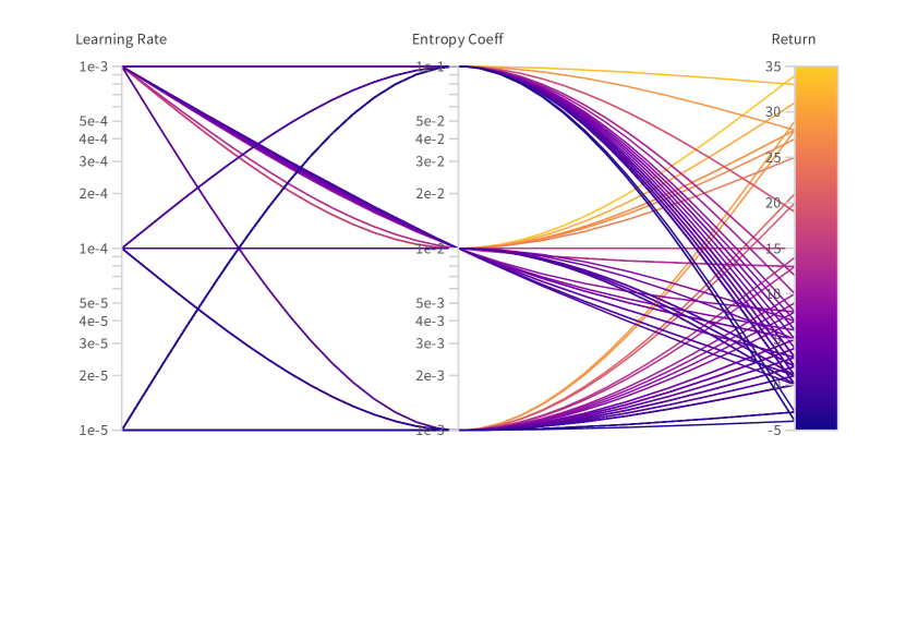
Figure 12: Parallel coordinates plot demonstrating effects of hyperparameters. This is for OC-PPO

Learning Rate	Entropy Coefficient	Final Returns
0.00001	0.83
	0.001	0.79
	0.1	0.86
0.0001	3.2
	0.001	5.67
	0.01	1.92
	0.1	0.83
0.001	12.67
	0.001	15.83
	0.01	12.22
	0.1	11.75

Table 9: Results for different learning rates and entropy coefficients for OC-PPO.

A.14 Full Procgen results

Learning curves across all tested Procgen environments and shown in Figure 13

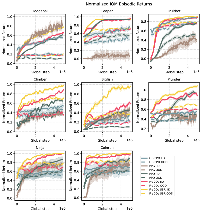
Figure 13: Learning curves for all methods on all Procgen environments

A.15 Success Criteria Hyperparameters

Environment	Minimum Success Returns
Four Rooms	0.97
Nine Rooms	0.60
Ramesh Maze	0.70
MetaGrid 14x14	0.95
BigFish	5
Climber	7
CoinRun	7.5
Dodgeball	5
FruitBot	7.5
Leaper	7
Ninja	7.5
Plunder	10

Table 10: Minimum Success Returns for Various Environments

A.16 Clustering Analysis

We compared different clustering methods and hyperparameters to ensure we were using a sensible combination. We desired our clustering method to have prediction functionality for new data and we didn’t want to specify the number of clusters. The only sensible clustering method which remained was HDBSCAN. Regardless we analysed others to ensure HDBSCAN was not significantly worse.

We first generated trajectories in the Nine Rooms environment, created embeddings using UMAP and then conducted clustering with various methods and parameters. Figures 14 provide visualisations of the results. We decided on HDBSCAN with minimum size of 15 and Eucledian distance metrics.

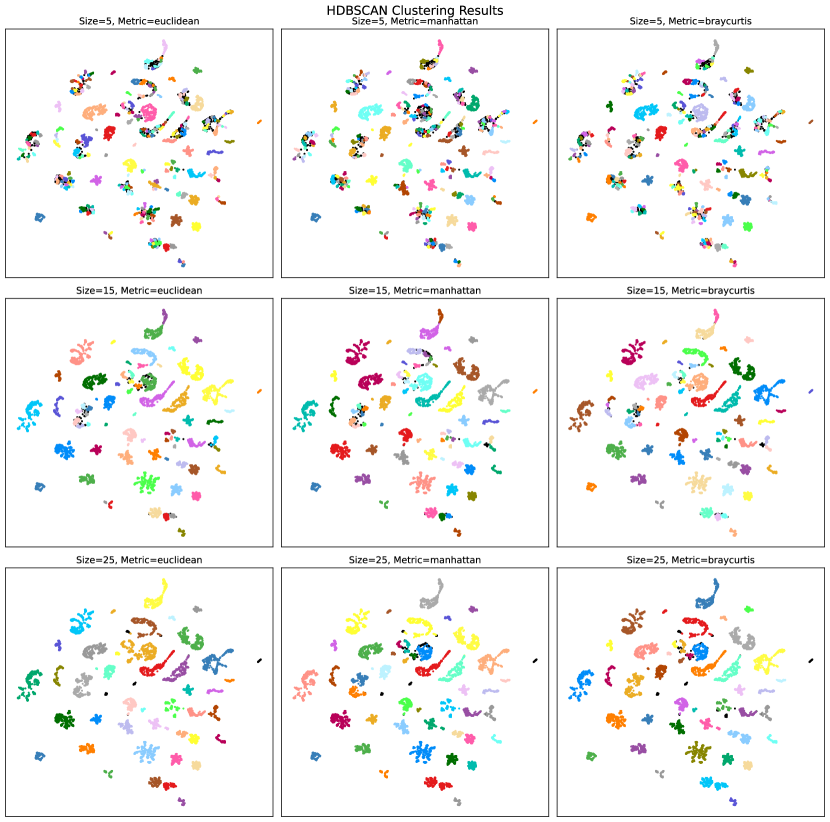
Figure 14: HDBSCAN clustering comparison

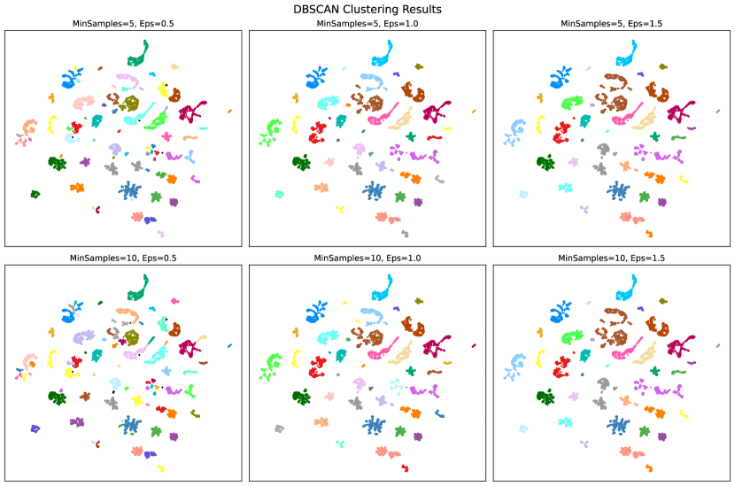
Figure 15: DBSCAN clustering comparison

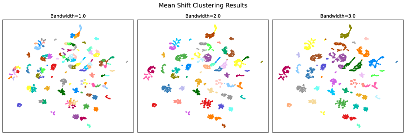
Figure 16: Mean Shift clustering comparison

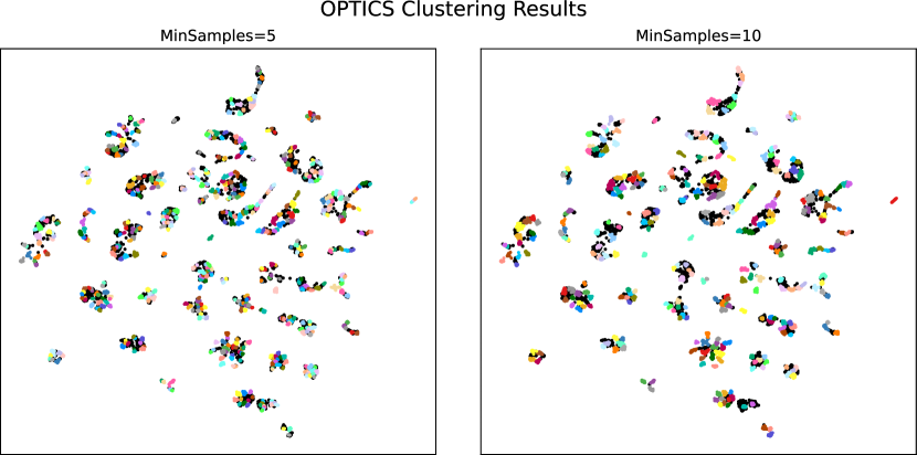
Figure 17: Optics clustering comparison

References

- Adolph and Robinson, (2013) Adolph, K. E. and Robinson, S. R. (2013). 403The Road to Walking: What Learning to Walk Tells Us About Development. In The Oxford Handbook of Developmental Psychology, Vol. 1: Body and Mind. Oxford University Press.
- Bacon et al., (2017) Bacon, P.-L., Harb, J., and Precup, D. (2017). The option-critic architecture. In Proceedings of the AAAI conference on artificial intelligence, volume 31.
- Barreto et al., (2019) Barreto, A., Borsa, D., Hou, S., Comanici, G., Aygün, E., Hamel, P., Toyama, D., Mourad, S., Silver, D., Precup, D., et al. (2019). The option keyboard: Combining skills in reinforcement learning. Advances in Neural Information Processing Systems, 32.
- Brunskill and Li, (2014) Brunskill, E. and Li, L. (2014). Pac-inspired option discovery in lifelong reinforcement learning. In International conference on machine learning, pages 316–324. PMLR.
- Campello et al., (2013) Campello, R. J., Moulavi, D., and Sander, J. (2013). Density-based clustering based on hierarchical density estimates. In Pacific-Asia conference on knowledge discovery and data mining, pages 160–172. Springer.
- Chevalier-Boisvert et al., (2023) Chevalier-Boisvert, M., Dai, B., Towers, M., de Lazcano, R., Willems, L., Lahlou, S., Pal, S., Castro, P. S., and Terry, J. (2023). Minigrid & miniworld: Modular & customizable reinforcement learning environments for goal-oriented tasks. arXiv preprint arXiv:2306.13831.
- Chollet, (2019) Chollet, F. (2019). On the measure of intelligence. arXiv preprint arXiv:1911.01547.
- Cobbe et al., (2020) Cobbe, K., Hesse, C., Hilton, J., and Schulman, J. (2020). Leveraging procedural generation to benchmark reinforcement learning. In International conference on machine learning, pages 2048–2056. PMLR.
- Cobbe et al., (2019) Cobbe, K., Klimov, O., Hesse, C., Kim, T., and Schulman, J. (2019). Quantifying generalization in reinforcement learning. In International conference on machine learning, pages 1282–1289. PMLR.
- Cobbe et al., (2021) Cobbe, K. W., Hilton, J., Klimov, O., and Schulman, J. (2021). Phasic policy gradient. In International Conference on Machine Learning, pages 2020–2027. PMLR.
- Dayan and Hinton, (1992) Dayan, P. and Hinton, G. E. (1992). Feudal reinforcement learning. Advances in neural information processing systems, 5.
- Dominici et al., (2011) Dominici, N., Ivanenko, Y. P., Cappellini, G., d’Avella, A., Mondì, V., Cicchese, M., Fabiano, A., Silei, T., Di Paolo, A., Giannini, C., et al. (2011). Locomotor primitives in newborn babies and their development. Science, 334(6058):997–999.
- Evans and Şimşek, (2023) Evans, J. B. and Şimşek, Ö. (2023). Creating multi-level skill hierarchies in reinforcement learning. arXiv preprint arXiv:2306.09980.
- Eysenbach et al., (2018) Eysenbach, B., Gupta, A., Ibarz, J., and Levine, S. (2018). Diversity is all you need: Learning skills without a reward function. arXiv preprint arXiv:1802.06070.
- Finn et al., (2017) Finn, C., Abbeel, P., and Levine, S. (2017). Model-agnostic meta-learning for fast adaptation of deep networks. In International conference on machine learning, pages 1126–1135. PMLR.
- Fox et al., (2017) Fox, R., Krishnan, S., Stoica, I., and Goldberg, K. (2017). Multi-level discovery of deep options. arXiv preprint arXiv:1703.08294.
- Frans et al., (2017) Frans, K., Ho, J., Chen, X., Abbeel, P., and Schulman, J. (2017). Meta learning shared hierarchies. arXiv preprint arXiv:1710.09767.
- Grant et al., (2018) Grant, E., Finn, C., Levine, S., Darrell, T., and Griffiths, T. (2018). Recasting gradient-based meta-learning as hierarchical bayes. arXiv preprint arXiv:1801.08930.
- Harutyunyan et al., (2019) Harutyunyan, A., Dabney, W., Borsa, D., Heess, N., Munos, R., and Precup, D. (2019). The termination critic. arXiv preprint arXiv:1902.09996.
- Heess et al., (2016) Heess, N., Wayne, G., Tassa, Y., Lillicrap, T., Riedmiller, M., and Silver, D. (2016). Learning and transfer of modulated locomotor controllers. arXiv preprint arXiv:1610.05182.
- Huang et al., (2022) Huang, S., Dossa, R. F. J., Ye, C., Braga, J., Chakraborty, D., Mehta, K., and AraÚjo, J. G. (2022). Cleanrl: High-quality single-file implementations of deep reinforcement learning algorithms. Journal of Machine Learning Research, 23(274):1–18.
- Kingma and Welling, (2013) Kingma, D. P. and Welling, M. (2013). Auto-encoding variational bayes. arXiv preprint arXiv:1312.6114.
- Kirk et al., (2021) Kirk, R., Zhang, A., Grefenstette, E., and Rocktäschel, T. (2021). A survey of generalisation in deep reinforcement learning. arXiv preprint arXiv:2111.09794.
- Klissarov et al., (2017) Klissarov, M., Bacon, P.-L., Harb, J., and Precup, D. (2017). Learnings options end-to-end for continuous action tasks. arXiv preprint arXiv:1712.00004.
- Konidaris and Barto, (2007) Konidaris, G. D. and Barto, A. G. (2007). Building portable options: Skill transfer in reinforcement learning. In IJCAI, volume 7, pages 895–900.
- Laird et al., (1987) Laird, J. E., Newell, A., and Rosenbloom, P. S. (1987). Soar: An architecture for general intelligence. Artificial intelligence, 33(1):1–64.
- Levy et al., (2017) Levy, A., Konidaris, G., Platt, R., and Saenko, K. (2017). Learning multi-level hierarchies with hindsight. arXiv preprint arXiv:1712.00948.
- Mann and Choe, (2013) Mann, T. A. and Choe, Y. (2013). Directed exploration in reinforcement learning with transferred knowledge. In European Workshop on Reinforcement Learning, pages 59–76. PMLR.
- Mazoure et al., (2022) Mazoure, B., Kostrikov, I., Nachum, O., and Tompson, J. J. (2022). Improving zero-shot generalization in offline reinforcement learning using generalized similarity functions. Advances in Neural Information Processing Systems, 35:25088–25101.
- McGovern and Sutton, (1998) McGovern, A. and Sutton, R. S. (1998). Macro-actions in reinforcement learning: An empirical analysis. Computer Science Department Faculty Publication Series, page 15.
- McInnes et al., (2018) McInnes, L., Healy, J., and Melville, J. (2018). Umap: Uniform manifold approximation and projection for dimension reduction. arXiv preprint arXiv:1802.03426.
- Mnih, (2016) Mnih, V. (2016). Asynchronous methods for deep reinforcement learning. arXiv preprint arXiv:1602.01783.
- Parr and Russell, (1997) Parr, R. and Russell, S. (1997). Reinforcement learning with hierarchies of machines. Advances in neural information processing systems, 10.
- Pateria et al., (2021) Pateria, S., Subagdja, B., Tan, A.-h., and Quek, C. (2021). Hierarchical reinforcement learning: A comprehensive survey. ACM Computing Surveys (CSUR), 54(5):1–35.
- Ramesh et al., (2019) Ramesh, R., Tomar, M., and Ravindran, B. (2019). Successor options: An option discovery framework for reinforcement learning. arXiv preprint arXiv:1905.05731.
- Riemer et al., (2018) Riemer, M., Liu, M., and Tesauro, G. (2018). Learning abstract options. Advances in neural information processing systems, 31.
- Rosenbloom and Newell, (1986) Rosenbloom, P. S. and Newell, A. (1986). The chunking of goal hierarchies: A generalized model of practice. Machine learning-an artificial intelligence approach, 2:247.
- Schulman et al., (2017) Schulman, J., Wolski, F., Dhariwal, P., Radford, A., and Klimov, O. (2017). Proximal policy optimization algorithms. arXiv preprint arXiv:1707.06347.
- Shannon, (1948) Shannon, C. E. (1948). A mathematical theory of communication. The Bell system technical journal, 27(3):379–423.
- Sutton and Barto, (2018) Sutton, R. S. and Barto, A. G. (2018). Reinforcement learning: An introduction. MIT press.
- Sutton et al., (1999) Sutton, R. S., Precup, D., and Singh, S. (1999). Between mdps and semi-mdps: A framework for temporal abstraction in reinforcement learning. Artificial intelligence, 112(1-2):181–211.
- Tessler et al., (2017) Tessler, C., Givony, S., Zahavy, T., Mankowitz, D., and Mannor, S. (2017). A deep hierarchical approach to lifelong learning in minecraft. In Proceedings of the AAAI Conference on Artificial Intelligence, volume 31.
- Towers et al., (2023) Towers, M., Terry, J. K., Kwiatkowski, A., Balis, J. U., Cola, G. d., Deleu, T., Goulão, M., Kallinteris, A., KG, A., Krimmel, M., Perez-Vicente, R., Pierré, A., Schulhoff, S., Tai, J. J., Shen, A. T. J., and Younis, O. G. (2023). Gymnasium.
- Zhang and Whiteson, (2019) Zhang, S. and Whiteson, S. (2019). Dac: The double actor-critic architecture for learning options. Advances in Neural Information Processing Systems, 32.