Influence of field mass and acceleration on entanglement generation
Abstract
We explore the entanglement dynamics of two detectors undergoing uniform acceleration and circular motion within a massive scalar field, while also investigating the influence of the anti-Unruh effect on entanglement harvesting. Contrary to the conventional understanding of the weak anti-Unruh effect, where entanglement typically increases, we observe that the maximum entanglement between detectors does not exhibit a strict monotonic dependence on detector acceleration. Particularly at low accelerations, fluctuations in the entanglement maxima show a strong correlation with fluctuations in detector transition rates. We also find that the maximum entanglement of detectors tends to increase with smaller field masses. Novelly, our findings indicate the absence of a strong anti-Unruh effect in (3+1)-dimensional massive scalar fields. Instead, thermal effects arising from acceleration contribute to a decrease in the detector entanglement maximum.
pacs:
04.70.Dy, 04.70.-s, 04.62.+vI Introduction
The Unruh effect posits that a uniformly accelerated detector with acceleration perceives the Minkowski vacuum as a thermal state at the Unruh temperature unruh1976notes . This temperature can also be accurately determined from the transition probability and the detailed equilibrium temperature when an accelerating Unruh-DeWitt detector is coupled with a massless field Hawking1979GeneralRA ; takagi1986vacuum ; crispino2008unruh . Recent studies have revealed that under special conditions, when the detector is coupled with a massive field, the transition probability and detailed equilibrium temperature are not directly proportional to the detector’s acceleration. This phenomenon has been termed the anti-Unruh effect brenna2016anti ; garay2016thermalization . Specifically, a decrease in the detector’s transition probability alongside an increase in acceleration is known as the weak anti-Unruh effect, while the associated decrease in the detailed equilibrium temperature is termed the strong anti-Unruh effect.
Local coupling between detectors and fields is of significant importance in various applications. When considering the first-order perturbative expansion of the time evolution operator for such local coupling processes, the entanglement of an initially entangled state undergoing accelerated motion tends to decrease due to thermal effects caused by acceleration fuentes2005alice ; alsing2006entanglement ; martin2009fermionic ; bruschi2012particle . However, in the presence of the anti-Unruh effect, the entanglement of both two-body entangled states li2018would and multi-body entangled states pan2020influence can actually increase. Furthermore, when moving to the second-order perturbative expansion of the time evolution operator, a pair of detectors that were initially unrelated can become entangled through local coupling with a vacuum field, even if they are spatially distant. This phenomenon is aptly termed “entanglement harvesting” reznik2003entanglement ; Zhang2020circ ; Gallock2021black ; chowdhury2022fate ; Pozas2015gta ; Tjoa2020Vacuum . This article specifically focuses on the entanglement harvesting process involving detectors.
The Unruh effect and the anti-Unruh effect exhibit opposite impacts on quantum entanglement, and their persistence in entanglement harvesting reflects directly on detector entanglement dynamics. Recent studies emphasize the significance of field mass in relation to the anti-Unruh effect garay2016thermalization ; wu2023conditions ; yan2023reveal . Consequently, there is considerable interest in exploring entanglement harvesting processes within massive fields, including considerations such as environmental interaction effects Zhou2021nyv ; chen2022entanglement , detector energy level gaps Maeso2022Entanglement ; Hu2022nxc , and high-dimensional spacetime yan2022effect . Our investigation delves into the role of field mass in the entanglement harvesting process involving detectors within a massive field, aiming to ascertain whether the anti-Unruh effect contributes to detector entanglement. In contrast to previous studies of detector entanglement dynamics in massive fields, we discuss in detail the influence of strong and weak anti-Unruh effects on entanglement generation in the evolution of detector dynamics. It is found that the time-delay effect induced by the mass of the field, as well as only the weak anti-Unruh effect has an effect on the entanglement generation in the evolution of the detector dynamics.
Typically, the Unruh effect pertains to detectors undergoing linear acceleration, but exploring the Unruh effect in circular motion is particularly intriguing due to the feasibility of achieving high accelerations required for experimental verification Bell1982qr . Furthermore, the temperature measured by detectors in circular motion exhibits similarities but also differences compared to the conventional Unruh temperature Biermann2020Unruh . Therefore, understanding the anti-Unruh effect in circular motion and its implications for entanglement harvesting is crucial salton2015acceleration ; liu2022does . Recent studies have examined entanglement dynamics in circular motion within massless Zhang2020circ , electromagnetic fields Pozas2016rsh ; Perche2022Harvesting , and other types of world lines Bozanic2023Correlation . In this context, we focus on elucidating the entanglement dynamics between detectors engaged in circular motion within a massive field, aiming to explore the contributions of the anti-Unruh effect to this process.
This paper is organized as follows. In the second section, we introduce the process of coupling two detectors to a vacuum field. Next, in the third section, we compare the entanglement dynamics of detectors when coupled to both a massless field and a massive field. The fourth section provides a detailed examination of the entanglement dynamics of detectors in circular motion. Subsequently, in the fifth section, we discuss the correlation between the anti-Unruh effect and the entanglement dynamics. Finally, we conclude the paper with a summary in the sixth section.
II Master equation
We study the entanglement dynamics of two uniformly accelerated two-level atoms, which are weakly coupled to fluctuating massless and massive scalar fields in vacuum. The Hamiltonian of the two detector can be expressed as audretsch1994spontaneous
| (1) |
where are operators of detectors and respectively, with being the Pauli matrices, and is the unit matrix. We assume that the excitation energy of the two detectors are the same, and labeled as . The interaction Hamiltonian between the detector and the vacuum scalar field can be written as
| (2) |
where is the coupling constant which is assumed to be small.
In the Born-Markov approximation, the master equation describing the dissipative dynamics of the two-detector subsystem can be written in the Gorini-Kossakowski-Lindblad-Sudarshan form as gorini1978properties ; lindblad1976generators ; breuer2002theory
| (3) |
where
| (4) |
with can be obtained by the Hilbert transform , i.e.,
| (5) |
where represents the principal value of the integral and is interpreted below, and
| (6) |
From the master equation (3), it is clear that the environment leads to decoherence and dissipation described by the dissipator such that the evolution of the quantum system is nonunitary on one hand, and it also gives rise to a modification of the unitary evolution term which incarnates in the Hamiltonian on the other hand.
III Entanglement change
Consider the two detectors separated by undergoing linear acceleration in the (3+1)-dimensional vacuum field. Their worldlines are
| (9) |
To accurately show the evolution of the density matrix of the detector, we need to calculate the correlation function of the massive and massless scalar fields.
For a massless scalar field,
| (10) |
where, represents the spacial component, and the superscripts and are omitted for the simplicity of the formula. The Fourier transformation of the correlation functions are
| (11) |
For the massive scalar field,
| (12) |
where . According to the word line (9), it is obtained Zhou2021nyv ,
| (13) |
and
| (14) |
Their Fourier transformation,
| (15) |
Note that for both massless and massive field is proportional to the excitation/deexcitation rate of the single detector, and it satisfies the KMS condition kubo1986brownian ; martin1959theory
| (16) |
where is the Unruh temperature perceived by the detector.
III.1 Entanglement dynamics
We study the entanglement dynamics of two uniformly accelerated two-level detectors, which are weakly coupled to fluctuating massless and massive scalar fields in the vacuum. For convenience, we work in the coupled basis
and obtain the following time evolution equations of the density matrix elements ficek2002entangled
| (17) |
where , , and .
Moreover, we just consider the effect of environment (the vacuum field) on quantum entanglement between two accelerated detectors, so the Hamiltonian for any single detector and vacuum contribution terms can be neglected, and we just need to consider the effect of dissipator . In order to eliminate the interaction between the two detectors caused by the environment, we let in Eq. (17). The computation of the additive environment leading term can be found in Ref. chen2022entanglement .
III.2 Entanglement generation
We investigate the entanglement generation between two initially separable uniformly accelerated detectors, and focus on the environment-induced interaction. According to the evolution equation of the density matrix elements (17), the density matrix elements affected by the environment-induced interatomic interaction in the coupled basis are and .
The concurrence which quantifies the amount of quantum entanglement of the bipartite entanglement state in the X-form state can be expressed as wootters1998entanglement ; tanas2004entangling
| (18) |
where
| (19) |
To calculate the entanglement dynamics of the system, assume that the initial state of the two-atom system is (). In the environment-induced interaction, the element of the density matrix will remain at zero. So the value of concurrence becomes . Entanglement can be generated at the neighborhood of the initial time when . The expression for is given by
| (20) |
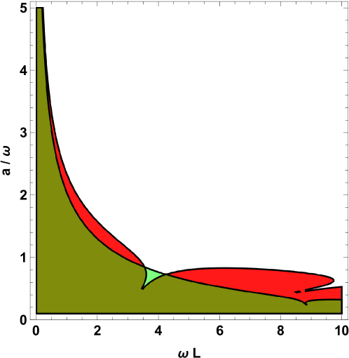
Fig. 1 shows the parameter space for entanglement generation when the environment-induced interaction between the detectors accelerated in the vacuum is considered. The estimated area of the entanglement region for massless and massive fields are and , respectively. It means that the parameter space for entanglement generation shrinks when the mass of the field is taken into account.
III.3 Entanglement degradation
Now, we discuss the degradation process of entanglement. The entanglement between the two detectors will gradually decrease after generation. From the previous sections, we know that three main factors affect the generation of entanglement, which is acceleration, field mass, and the spatial distance between detectors. In this paper, we consider the influence of acceleration and field mass on the detectors’ ability to extract entanglement when the spatial distance is fixed.
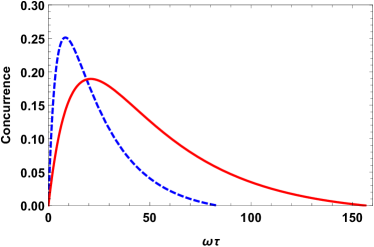
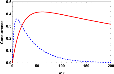
Fig. 2 shows the evolution of the entanglement harvesting of the detectors in vacuum. Regardless of the influence of the field mass and acceleration, the entanglement decreases with the increase of time after a sufficient interaction between detectors and vacuum. The amount of entanglement will first increase and then decrease with time. The entanglement drops to zero when the interaction time is long enough. Firstly, focus on the left panel of Fig. 2, where the red dotted line represents the entanglement evolution with the paramenter . When the mass , the change of entanglement returns to the case for the massless field. In particular, the presence of field mass can slow down entanglement degradation, which may be related to the time delay effect caused by field mass Zhou2021nyv . The time delay effect means, compared with the massless field, the entanglement evolution in the massive case is generally slower. The right panel of Fig. 2 explains the entanglement evolution process when the acceleration is small. Compared with the left figure, the entanglement generation in the dynamical evolution of the detectors increases for both massless and massive fields.
IV Circular motion
In this section, we will analyze the entanglement dynamics for two atoms in circular motion, and compare them with the uniform acceleration case.
We first give the trajectory of circular motion,
| (21) |
where is the radius of the circular trajectory in a plane parallel to the xy-plane, is the angular velocity which can be either positive or negative in the circular motion, and denotes the Lorentz factor. In the detector’s frame, the magnitude of acceleration satisfied with the magnitude of linear velocity . Substituting the trajectory into the Wightman function, we obtain
| (22) |
Then, substituting the Wightman function into Eq. (8), we get
| (23) |
For the massive field case, the Wightman function is Maeso2022Entanglement
| (24) |
We can also use the circular motion trajectory, and get the Wightman function for the circular motion case
| (25) |
Their Fourier transformations
| (26) |
The expressions in Eqs. (23) and (26) do not have analytic form, so we need to perform them numerically.
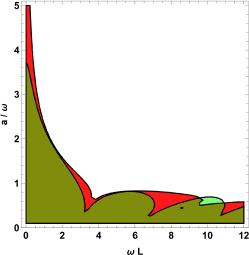
The entanglement region for the circular motion case is shown in Fig. 3. Comparing it with Fig. 1, we find that the shapes of the entanglement region for circular and uniform line acceleration are similar, but the estimated area of the entanglement region for the circular motion is smaller than the uniform line acceleration case.
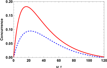
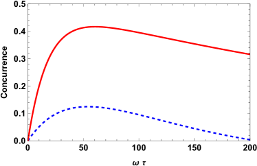
Fig. 4 shows the entanglement dynamics for the circular motion case. For the same energy gap and distance , the amount of entanglement generated from the circular motion is less than the entanglement generated from the uniform acceleration motion. When the acceleration is smaller, this difference becomes bigger, because both cases approach the entanglement generation for the static case.
V Anti-Unruh phenomenon and field mass
From the right panels of Fig. 2 and Fig. 4, the detectors in the massive field can harvest more entanglement when the acceleration is small. As discussed in some previous studies, the anti-Unruh can increase entanglement among entangled states for both bipartite states li2018would and multi-body states pan2020influence , which makes us wonder if the anti-Unruh effect can help generating entanglement between detectors in their dynamical evolution process liu2022does . To solve this problem, we analyze the conditions for the anti-Unruh effect in detail using the methods of Refs. garay2016thermalization ; wu2023conditions .
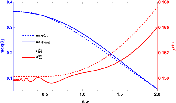
Figure 5 illustrates the change in detector transition rate and entanglement maxima (peaks at a given acceleration in Fig. 2 and 4) with acceleration for linearly accelerated and circular motions. For linearly accelerated motion, the fluctuations in the transition rate at small accelerations demonstrate the presence of the weak anti-Unruh effect. However, this fluctuation has no effect on the degradation of entanglement. For the circular motion, the weak anti-Unruh effect is absent and has no effect on the entanglement degradation. Therefore the Unruh and anti-Unruh effects are not necessarily related to the degradation of entanglement.
Consider two different limits for the field mass: the large mass limit and the small mass limit. Note that the small mass limit is not , and the large one is not . A detailed discussion of these two limits can be found in Ref. takagi1986vacuum ; garay2016thermalization .
Let us begin with the large mass limit. In order to show the dependence of the field mass more clearly, the Fourier transformation for the green function of the massive scalar field is first calculated. Substitute Eq. (13) into Eq. (8) to get,
| (27) |
The asymptotic expansion of the Bessel function for large values of its argument is given as
| (28) |
and we use only the leading order term in our calculation, that is the first term in Eq. (28). It can be justified under the condition
| (29) |
Thus, we get the following response function in the large mass limit,
| (30) |
We are at this point going to expand the second class of modified Bessel functions to the second order of the curly brackets in Eq. (28), and the asymptotic behavior of the response function in the limit of a small mass is given by
| (31) |
This is justified under the condition
| (32) |
which is roughly, but not quite, the opposite of Eq. (29).
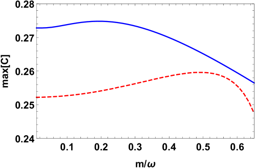
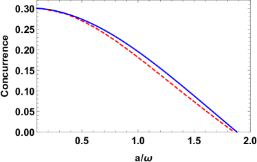
Figure 6 illustrates the change of the entanglement maximum with the field mass for linear acceleration and circular motions. The entanglement captured by the detector increases at small accelerations, but decreases as the mass increases further. In order to check whether the anti-Unruh effect plays a role in this process, we calculated the KMS temperatures perceived by the detector in uniform acceleration and the detector in circular motion.
The KMS temperatures of the field can be calculated from the ratio between the excitation and deexcitation rates of the detectors takagi1986vacuum ,
| (33) |
where . The response function is also proportional to the transition rate of the detector, when it interacts with a (3+1) dimensional massive field. So we get,
| (34) |
Thus, we can see that the strong anti-Unruh effect does not occur in both the small mass limit and the large mass limit.
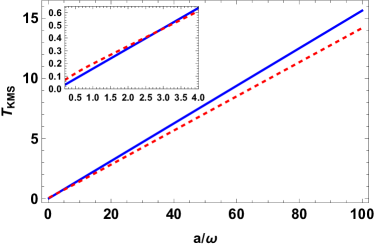
The left-hand panel of Fig. 7 shows the change of entanglement with acceleration for a fixed spatial interval and evolution time. The detector extracts more entanglement for two atoms in the uniform acceleration than that in the circular motion. Based on the difference of the temperature induced by acceleration for circular and linear acceleration motions Biermann2020Unruh and the effect of thermal field on the entanglement of quantum entangled states Dai2015ota ; barman2021radiative . We understand that circular motion produces less entanglement because circular motion produces a higher Unruh temperature at smaller accelerations.
The right-hand panel of Fig. 7 illustrates the relation between the KMS temperature and the acceleration for both circular and linear motion cases. Remarkably, the KMS temperature for linear accelerated detectors is proportional to the acceleration and is irrelevant with the field mass. There is no analytic expression for the KMS temperature for circular accelerated detectors, but it still increases with the increasing acceleration Biermann2020Unruh . So there is no appearance of the strong anti-Unruh effect in the whole process.
On the other hand, when the acceleration is small, the circularly accelerated detectors feel a higher temperature compared with the linear acceleration case; when the acceleration is large, detectors with linearly accelerated motions feel higher temperature. The results are consistent with previous results like that in Ref. Biermann2020Unruh . Therefore, during entanglement harvesting, the weak anti-Unruh effect has an impact on the entanglement dynamics of the detector, but the strong anti-Unruh effect does not occur and does not contribute.
VI Conclusion
We explore the entanglement dynamics between two detectors undergoing uniform linear acceleration and circular motion within a massive scalar field. First, we find that under linear acceleration, detectors are more readily entangled in a massless scalar field compared to a massive scalar field. Additionally, we analyze the evolution of entanglement between detectors in conjunction with their intrinsic time scales. Our findings reveal that detectors exhibit greater entanglement capture at lower accelerations, observed in both massive and massless scalar field scenarios. Furthermore, we observe a noticeable time-delay effect attributable to mass production.
Next, we analyze the entanglement generation process between detectors during circular motion. Despite the similarity in the entanglement-generating region’s profile compared to linear acceleration, circular motion is less conducive to generating entanglement compared to linear acceleration. We then compare the entanglement dynamics between detectors experiencing acceleration during circular motion versus linear acceleration. Our results indicate that detectors in linear acceleration yield more entanglement when the acceleration is small. This can be attributed to the linearly accelerating detector perceiving a lower KMS temperature under mild acceleration. Similarly, we find that in circular motion scenarios, detectors also harvest more entanglement with lower acceleration, regardless of whether the scalar field is massive or massless.
Finally, we investigate the relationship between entanglement generation in the dynamical evolution of the detectors and the mass of the field. Our findings reveal a certain increase in the maximum entanglement between detectors when the field mass is small. However, this increase is not attributed to the strong anti-Unruh effect. We begin by defining the anti-Unruh effect and determine that there is no presence of the strong anti-Unruh effect throughout the process. However, the weak anti-Unruh effect does impact the entanglement dynamics of the detector. Interestingly, the influence of the weak anti-Unruh effect differs from the conventional understanding (where entanglement increases), as the entanglement between detectors does not exhibit a strictly monotonic dependence on acceleration.
Acknowledgements.
Pan and Yan contributed equally to this work. This work is supported by National Natural Science Foundation of China (NSFC) with Grant No. 12375057 and the Fundamental Research Funds for the Central Universities, China University of Geosciences (Wuhan).References
- (1) W. G. Unruh, Notes on black-hole evaporation, Phys. Rev. D 14, 870 (1976).
- (2) B. S. DeWitt, S. Hawking, and W. Israel, General Relativity: An Einstein Centenary Survey (Cambridge University Press Cambridge, England, 1979).
- (3) S. Takagi, Prog. Theor. Phys. Suppl. 88, 1 (1986).
- (4) L. C. B. Crispino, A. Higuchi, and G. E. A. Matsas, Rev. Mod. Phys. 80, 787 (2008).
- (5) W. G. Brenna, R. B. Mann, and E. Martín-Martínez, Phys. Lett. B 757, 307 (2016).
- (6) L. J. Garay, E. Martín-Martínez, and J. de Ramon, Phys. Rev. D 94, 104048 (2016).
- (7) I. Fuentes-Schuller and R. B. Mann, Phys. Rev. Lett. 95, 120404 (2005).
- (8) P. M. Alsing, I. Fuentes-Schuller, R. B. Mann, and T. E. Tessier, Phys. Rev. A 74, 032326 (2006).
- (9) E. Martín-Martínez and J. León, Phys. Rev. A 80, 042318 (2009).
- (10) D. E. Bruschi, A. Dragan, I. Fuentes, and J. Louko, Phys. Rev. D 86, 025026 (2012).
- (11) T. Li, B. Zhang, and L. You, Phys. Rev. D 97, 045005 (2018).
- (12) Y. Pan and B. Zhang, Phys. Rev. A 101, 062111 (2020).
- (13) B. Reznik, Found. Phys. 33, 167 (2003).
- (14) J. Zhang and H. Yu, Phys. Rev. D 102, 065013 (2020).
- (15) K. Gallock-Yoshimura, E. Tjoa, and R. B. Mann, Phys. Rev. D 104, 025001 (2021).
- (16) P. Chowdhury and B. R. Majhi, JHEP 05, 025 (2022).
- (17) A. Pozas-Kerstjens and E. Martín-Martínez, Phys. Rev. D 92, 064042 (2015).
- (18) E. Tjoa and E. Martín-Martínez, Phys. Rev. D 101, 125020 (2020).
- (19) D. Wu, J.-c. Yang, and Y. Shi, Eur. Phys. J. C 83, 1110 (2023).
- (20) J. Yan, B. Zhang and Q. Cai, arXiv, 2311.04610.
- (21) Y. Zhou, J. Hu, and H. Yu, JHEP 09, 088 (2021)
- (22) Y. Chen, J. Hu, and H. Yu, Phys. Rev. D 105, 045013 (2022).
- (23) H. Maeso-García, T. R. Perche, and E. Martín-Martínez, Phys. Rev. D 106, 045014 (2022)
- (24) H. Hu, J. Zhang, and H. Yu, JHEP 05, 112 (2022).
- (25) J. Yan and B. Zhang, JHEP 10, 051 (2022).
- (26) J. S. Bell and J. M. Leinaas, Nucl. Phys. B 212, 131 (1983).
- (27) S. Biermann, S. Erne, C. Gooding, J. Louko, J. Schmiedmayer, W. G. Unruh, and S. Weinfurtner, Phys. Rev. D 102, 085006 (2020).
- (28) G. Salton, R. B. Mann, and N. C. Menicucci, New J. Phys. 17, 035001 (2015).
- (29) Z. Liu, J. Zhang, R. B. Mann, and H. Yu, Phys. Rev. D 105, 085012 (2022).
- (30) A. Pozas-Kerstjens and E. Martin-Martinez, Phys. Rev. D 94, 064074 (2016).
- (31) T. R. Perche, C. Lima, and E. Martín-Martínez, Phys. Rev. D 105, 065016 (2022).
- (32) L. Bozanic, M. Naeem, K. Gallock-Yoshimura, and R. B. Mann, Phys. Rev. D 108, 105017 (2023).
- (33) J. Audretsch and R. Müller, Phys. Rev. A 50, 1755 (1994).
- (34) V. Gorini, A. Frigerio, M. Verri, A. Kossakowski, and E. C. G. Sudarshan, Rept. Math. Phys. 13, 149 (1978).
- (35) G. Lindblad, Commun. Math. Phys. 48, 119 (1976).
- (36) H.-P. Breuer, F. Petruccione, et al., The theory of open quantum systems (Oxford University Press on Demand, 2002).
- (37) N. D. Birell and P. C. W. Davies, Quantum Fields in Curved Space (Cambridge University Press, 1982).
- (38) R. Kubo, Science 233, 330 (1986)
- (39) P. C. Martin and J. Schwinger, Phys. Rev. 115, 1342 (1959).
- (40) Z. Ficek and R. Tanaś, Phys. Rept. 372, 369 (2002).
- (41) W. K. Wootters, Phys. Rev. Lett. 80, 2245 (1998).
- (42) R. Tanaś and Z. Ficek, Journal of Optics B: Quantum and Semiclassical Optics 6, S90 (2004).
- (43) Y. Dai, Z. Shen, and Y. Shi, JHEP 09, 071 (2015).
- (44) S. Barman and B. R. Majhi, JHEP 03, 245 (2021).