Confidence Calibration of Classifiers with Many Classes

Abstract

For classification models based on neural networks, the maximum predicted class probability is often used as a confidence score. This score rarely predicts well the probability of making a correct prediction and requires a post-processing calibration step. However, many confidence calibration methods fail for problems with many classes. To address this issue, we transform the problem of calibrating a multiclass classifier into calibrating a single surrogate binary classifier. This approach allows for more efficient use of standard calibration methods. We evaluate our approach on numerous neural networks used for image or text classification and show that it significantly enhances existing calibration methods. Our code can be accessed at the following link: https://github.com/allglc/tva-calibration.

1 Introduction

The considerable performance increase of modern deep neural networks (DNNs) and their potential deployment in real-world applications has made reliably estimating the probability of wrong decisions a key concern. When such components are expected to be embedded in safety-critical systems (e.g., medical or transportation), estimating this probability is crucial to mitigate catastrophic behavior. One way to address this question is to treat it as an uncertainty quantification problem [2, 12], where the uncertainty value computed for each prediction is considered as a confidence. This confidence can be used to reject uncertain decisions proposed by the DNN [13], for out-of-distribution detection [22], or to control active learning [34] or reinforcement learning based systems [76]. When confidence values reliably reflect the true probability of correct decisions, i.e., their accuracy, a predictive system is said to be calibrated. In this case, confidence values can be used as a reliable control for decision-making.

We are interested in producing an uncertainty indicator for decision problems where the input is high dimensional and the decision space large, typically classifiers with tens to thousands of classes. For this kind of problem, DNNs are common predictors, and their outputs can be used to provide an uncertainty value at no cost, i.e., without necessitating heavy estimation such as Bayesian sampling [15] or ensemble methods [33]. Indeed, most neural architectures for classification instantiate their decision as a softmax layer, where the maximum value can be interpreted as the maximum of the posterior probability and, therefore, as a confidence. Unfortunately, uncertainty values computed in this way are often miscalibrated. DNNs have been shown to be over-confident [17], meaning their confidence is higher than their accuracy: predictions with 90% confidence might be correct only 80% of the time. A later study [44] suggests that model architecture impacts calibration more than model size, pre-training, and accuracy. For ImageNet classifiers, the accuracy and the number of model parameters are not correlated to calibration, but model families are [11].

These studies show that it is difficult to anticipate the calibration level of confidence values computed directly from DNNs and exhibit the benefits of a complementary post-processing calibration. This calibration process can be seen as a learning step that exploits data from a calibration set, distinct from the training set, and is used to learn a function that maps classifier outputs into better-calibrated values. This process is typically lightweight and decoupled from the issue of improving model performance. A standard baseline for post-processing calibration is Temperature Scaling [17], where the penultimate logit layer is scaled by a coefficient optimized on the calibration set.

Many post-processing calibration methods have been developed for binary classification models [50, 69, 70]. Applying these methods to multiclass classifiers requires some adaptation. One standard approach reformulates the multiclass setting into many One-versus-All binary problems (one per class) [70]. One limitation of this approach is that it does not scale well. When the number of classes is large, the calibration data is divided into highly unbalanced subsets that do not contain enough positive examples to solve the One-versus-All binary problems. Other methods based on Platt scaling [50] involve learning a set of parameters whose size grows with the number of classes. For problems with many classes, they tend to overfit, as we demonstrate in this work.

The main idea of our work is to reformulate the multiclass confidence estimation into a single binary problem. This problem can be phrased as the unique question: "Is the prediction correct?". In this formulation, the confidence score is defined as the maximum class probability of the binary problem that outputs $1$ if the predicted class is correct and $0$ otherwise. The intent is that the confidence score accurately describes whether the prediction is correct, regardless of the class. We show that this novel approach, which we call Top-versus-All (TvA), significantly improves the performance of standard calibration methods: Temperature and Vector Scaling [17], Dirichlet Calibration [29], Histogram Binning [69], Isotonic Regression [70], Beta Calibration [28], and Bayesian Binning into Quantiles [46]. We also introduce a simple regularization for Vector Scaling or Dirichlet Calibration that mitigates overfitting when the number of classes is high relative to the calibration data size. We conduct experiments on multiple image and text classification datasets and many pre-trained models.

Our main contributions are the following:

• We discuss four issues of the standard approach to confidence calibration.

• To solve these issues, we develop the Top-versus-All approach to confidence calibration of multiclass classifiers, transforming the problem into a single binary classifier’s calibration. This straightforward reformulation enables more efficient use of existing calibration methods, achieved with minimal modifications to the methods’ original algorithms.

• Applied to scaling methods for calibration (such as Temperature Scaling), TvA allows the use of the binary cross-entropy loss, which is more efficient in decreasing the confidence of wrong predictions and leads to stronger gradients in the case of Temperature Scaling.
  Applied to binary methods for calibration (such as Histogram Binning), TvA significantly improves their performance and makes them accuracy-preserving.

• We demonstrate our approach’s scalability and generality with extensive experiments on image classification with state-of-the-art models for complex datasets and on text classification with Pre-trained Language Models (PLMs) and Large Language Models (LLMs).

2 Related work

Calibration

There are various notions of multiclass calibration. One can consider confidence [17], class-wise [28], top-$r$ [19], top-label [18], decision [75], projection smooth [16], or strong [60, 65] calibration. For recent surveys, we refer to [10] and [63]. In this work, we focus on confidence calibration and not on the calibration of the full probability vector. Indeed, confidence calibration is useful for many applications that only require a single confidence value: selective classification [13], out-of-distribution detection [22], or active learning [34]. For these applications, stronger notions of calibration are both difficult and useless. Also, class-wise calibration metrics do not appropriately scale to large numbers of classes, a setting we consider in this work, as explained in Appendix E.

Metrics

Several metrics have been proposed to quantify calibration error. The most common is the Expected Calibration Error (ECE) [46] (see Equation 2). ECE has flaws: the estimation quality is influenced by the binning scheme, and it is not a proper scoring rule [14, 60, 48]. Despite its flaws, it remains the standard comparison metric for confidence calibration. Variants of ECE have also been developed: classwise-ECE [29], ECE with equal mass bins [48, 44], or top-label-ECE, which adds a conditioning on the predicted class [18]. The Brier score [4] is also used to measure calibration. The proximity-informed expected calibration error (PIECE) evaluates the miscalibration due to proximity bias [68]. We mainly use the standard ECE in this work, and the Appendix contains more metrics.

Training calibrated networks

Several solutions have been proposed in the literature to improve calibration by training neural networks in specific ways, generally by making use of a new loss term [31, 58, 26, 6, 5]. While these methods directly optimize calibration during the training phase of the networks, they require a high development time, often compromise accuracy, and are not adapted to pre-trained foundation models. That is why we prefer to focus on calibrating already-trained models.

Post-processing (or post-hoc) calibration methods

Another approach is to calibrate already-trained models. This lowers the development time by decoupling accuracy optimization and calibration. In this paper, we divide post-hoc calibration methods into two categories: scaling and binary.
Scaling methods are derived from Platt scaling [50] and optimize some parameters to scale the logits. Temperature Scaling [17] is a popular simple post-processing calibration method. The logits vector is scaled by a coefficient, which modifies the probability vector. Vector Scaling [17] is more expressive and has good performance in many cases [17, 48, 29]. Matrix Scaling can also be considered for more expressiveness but is difficult to apply without overfitting [17]. Dirichlet Calibration [29] proposes a regularization strategy for Matrix Scaling. [72] developed Ensemble Temperature Scaling. Scaling can be combined with binning [30]. Besides logits or probabilities, features can also be used [35].
Another family of methods tackles binary classification. We designate them as binary methods. Histogram Binning [69] divides the prediction into $B$ bins according to the predicted probability. For each bin, a calibrated probability is computed from the calibration data. The probability becomes discrete: it can only take $B$ values. With some modifications, it outperforms scaling methods [18, 49]. Isotonic Regression [70] learns a piecewise constant function to remap probabilities. Bayesian Binning into Quantiles [46] brings Bayesian model averaging to Histogram Binning. Beta Calibration [28] uses a beta distribution to obtain a calibration mapping.
Our work reformulates the multiclass calibration problem and allows more efficient use of all these calibration methods, with little to no change in their algorithms.

Multiclass to Binary

Using binary calibration methods for a multiclass classifier requires adapting the multiclass setting. This is usually done with a One-versus-All approach [70, 17]. The multiclass setting is decomposed into $L$ One-versus-All independent problems: one binary problem for each class. [18] introduce the notion of top-label calibration, i.e., confidence calibration with additional conditioning on the predicted class (top-label). They describe a general multiclass-to-binary framework to develop top-label calibrators. [6] derive $L(L-1)/2$ pairwise binary problems. The approach requires training the classifier from scratch, and its performance decreases with the number of classes. Our work tackles this multiclass-to-binary research problem. Contrary to [6], the One-versus-All approach [70] and top-label calibrators [18], our approach works well for problems with many classes. The methods I-Max [49] and IRM [72] use a shared class-wise strategy to compute a single calibrator. The calibrator is applied to all class probabilities separately, so the class probabilities ranking and prediction might change. In contrast, TvA applied to binary methods rescales the confidence after the class prediction is made. I-Max and IRM consider the full class probabilities vectors, while TvA only considers confidence values. Also, they build on top of Histogram Binning and Isotonic Regression, respectively, while we apply our approach to many calibration methods. A concurrent work building on an intuition similar to ours derives a calibration method based on a Correctness-Aware Loss [38]. Appendix C discusses the differences between our approach and others.

3 Problem setting

3.1 Background

Confidence calibration of a classifier

We consider the classification problem where an input $x$ is associated with a class label $y\in\mathcal{Y}=\{1,2,...,L\}$. The neural network classifier $f$ provides a class prediction from a final softmax layer $\sigma$ that transforms intermediate logits $z$ into probabilities. The classifier prediction is the most probable class $\hat{y}=\arg\max_{k\in\mathcal{Y}}f_{k}(x)$ with $f_{k}(x)$ referring to the probability of class $k$, and the confidence score defined as $s=\max_{k\in\mathcal{Y}}f_{k}(x)$. Note that we use the term confidence to denote the maximum class probability. With $y$ the real label, we consider the confidence calibration definition from [17] that says that the classifier $f$ is calibrated if:

$$P(\hat{y}=y|s=p)=p,\quad\forall p\in[0,1]$$ (1)

where the probability is over the data distribution. Equation (1) expresses that the probability of being correct when the confidence is around $p$ is indeed $p$. For instance, if we consider the set of predictions with a confidence of $90\%$, they should be correct $90\%$ of the time. The conditional probability of (1) is not rigorously defined mathematically (the event $\{s=p\}$ has zero probability), and interval-based empirical estimators are often used to define metrics capable of evaluating how well (1) is satisfied. This is the case of ECE, which approximates the calibration error by partitioning the confidence distribution into $B$ bins. The absolute difference between the accuracy and confidence is computed for each subset of data in the bins. The final value is a weighted sum of the differences of each bin.

$$\text{ECE}=\sum_{b=1}^{B}\frac{n_{b}}{N}|\text{acc}(b)-\text{conf}(b)|$$ (2)

Where $n_{b}$ is the number of samples in bin $b$, $N$ is the total number of samples, $\text{acc}(b)$ is the accuracy in bin $b$, and $\text{conf}(b)$ is the average confidence in bin $b$. ECE can be interpreted visually by looking at diagrams such as those of Figure 1: ECE computes the sum of the red bars (difference between bin accuracy and average confidence) weighted by the proportion of samples in the bin.

Post-processing calibration methods

We are considering the scenario where a classifier has already been trained, and the objective is to enhance its calibration. Post-processing calibration methods aim to remap the classifier probabilities to better-calibrated values without modifying the classifier. They typically use a calibration set different from the training set to optimize parameters or learn a function. We note the calibration data $D_{cal}=\{(x_{i},y_{i})\}_{i=1}^{N}$. We focus on post-processing calibration because it enables better utilization of off-the-shelf models and separates model training (optimized for accuracy) from calibration. These advantages significantly reduce the development cost of obtaining a well-performing and well-calibrated model, contrary to optimizing calibration during training. We categorize the post-processing calibration techniques considered in this paper into two groups: scaling methods and binary methods.

3.2 Issues related to current approaches

Behavior of current scaling methods

Scaling methods for calibration optimize one or more coefficients that scale the logits vector to minimize on calibration data the cross-entropy loss defined as $l_{CE}=-\sum_{k=1}^{L}1_{k=y}\cdot\log(f_{k}(x))=-\log(f_{y}(x))$. Minimizing $l_{CE}$ therefore increases the probability of the true class. We can distinguish two cases to understand what happens during the optimization: whether the prediction $\hat{y}$ is correct or not. In the first case, the confidence score is $s=f_{y}(x)$: minimizing $l_{CE}$ increases the confidence $f_{y}(x)$. In the second case, the prediction is incorrect, which implies that $f_{y}(x)<s$. Minimizing $l_{CE}$ increases the probability of the true class $f_{y}(x)$ but does not directly change the confidence (because $s\neq f_{y}(x)$). Instead, the confidence (which was attributed to a wrong class) is indirectly lowered through the softmax normalization.

. $\hookrightarrow$ Issue 1: Cross-entropy loss only indirecly lowers confidence in wrong predictions.

We identified another issue of some scaling methods. By design, the number of parameters optimized by Vector Scaling and Dirichlet Calibration grows with the number of classes. When the number of classes is high, these methods overfit the calibration set as shown in Figure 3.

. $\hookrightarrow$ Issue 2: Vector Scaling and Dirichlet Calibration overfit calibration sets with many classes.

One-versus-All approach for binary methods

The One-versus-All (OvA) calibration approach [70] allows adapting calibration methods for binary classifiers to multiclass classifiers. To do so, it decomposes the calibration of multiclass classifiers into sets of $L$ binary calibration problems: one for each class $k$. For each problem, the considered probability is $f_{k}(x)$, and the associated label $1_{y=k}\in\{0,1\}$. When calibrating a classifier from data, each binary problem is highly imbalanced with a ratio between positive and negative examples equal to $\frac{1}{L-1}$ if the classes are equally sampled. For instance, for ImageNet, the ratio is 1/999: out of 25000 examples, only 25 have a positive label.

. $\hookrightarrow$Issue 3: OvA approach leads to highly imbalanced binary problems.

At test time, each of the $L$ class probabilities is calibrated by a separate calibration model. The resulting probability vector can be normalized to ensure a unit norm. Because each probability is calibrated independently, their ranking can change, thus modifying the predicted class. In Table 9, we see that accuracy is often negatively impacted in practice.

. $\hookrightarrow$Issue 4: OvA approach can change the predicted class and negatively impact the accuracy.

4 Top-versus-All approach to confidence calibration

Algorithm 1 Top-versus-All approach to confidence calibration

Input:

$D_{cal}$: $\{(x_{i},y_{i})\}_{i=1}^{N}$ the calibration data

$f$: the multiclass classifier

$g$: a calibration function $\triangleright$ e.g., Temperature Scaling

Preprocessing:

$\hat{y_{i}}\leftarrow\arg\max_{k\in\mathcal{Y}}f_{k}(x_{i})$ $\triangleright$ Compute class predictions

$y^{b}_{i}\leftarrow 1_{\mathrm{\hat{y_{i}}=y_{i}}}$ $\triangleright$ Compute predictions correctness

$f^{b}\leftarrow\max_{k\in\mathcal{Y}}f_{k}$ $\triangleright$ Create surrogate binary classifier

$D^{\text{\tiny TvA}}_{cal}\leftarrow\{(x_{i},y^{b}_{i})\}_{i=1}^{N}$ $\triangleright$ Build binary calibration set

Learn calibration function:

Learn $g$ to calibrate the surrogate binary classifier $f^{b}$ on $D^{\text{\tiny TvA}}_{cal}$

Inference:

Use $g$ to calibrate the confidences of the original multiclass classifier $f$

4.1 General presentation

In the calibration definition (1) and the standard ECE metrics, only the confidence, i.e., the maximal probability, reflects the likelihood of making an accurate prediction. The probabilities of other classes are not taken into account. However, the standard approach to calibration uses the entire set of probabilities, not just confidence, which introduces unnecessary complexity. We aim to simplify the process by reformulating the problem of calibrating multiclass classifiers into a single binary problem. This problem can be phrased as: "Is the prediction correct?". In this setting, we do not calibrate the predicted probabilities vector but only a scalar: the confidence. The remaining probabilities are discarded. This is equivalent to calibrating a surrogate binary classifier that predicts whether the class prediction is correct. Since this correctness classifier only considers the maximal probability versus all others, we call our approach Top-versus-All (TvA).

Replacing the standard approach by TvA is straightforward. Given the standard calibration data $D_{cal}=\{(x_{i},y_{i})\}_{i=1}^{N}$, we add a few data preprocessing steps. First, compute the class predictions $\hat{y}$ and their correctness: $y^{b}=1_{\hat{y}=y}$. Second, create the surrogate binary classifier $f^{b}(x)=\max_{k\in\mathcal{Y}}f_{k}(x)$. Finally, build the calibration set for the surrogate binary classifier:

$$D^{\text{\tiny TvA}}_{cal}=\{(x_{i},y^{b}_{i})\}_{i=1}^{N}$$ (3)

After this preprocessing, we choose a standard calibration function $g$, e.g., Temperature Scaling, to calibrate the surrogate binary classifier. The learning of the calibration function follows its original underlying algorithm but uses the modified calibration data $D^{\text{\tiny TvA}}_{cal}$. The learned calibration function is then applied to the confidences of the original multiclass classifier. Algorithm 1 describes our approach. In the Appendix, Algorithm 3 provides more details and highlights differences with the standard approach of Algorithm 2.

After this general presentation, we explain how TvA impacts the two categories of calibration methods, scaling and binary, in Subsections 4.2 and 4.3, respectively. We also justify its behavior.

4.2 Top-versus-All approach for scaling methods

Because our Top-versus-All setting reformulates the calibration of multiclass classifiers into a binary problem, the natural loss is the binary cross-entropy:

$$l_{BCE}=-\big{(}y^{b}\cdot\log s+(1-y^{b})\cdot\log(1-s)\big{)}$$ (4)

Minimizing this loss results in confidence estimates that more accurately describe the probability of being correct, regardless of the $L-1$ less likely class predictions. Using the binary cross-entropy as a calibration loss makes an important difference compared to the usual multiclass cross-entropy. The cross-entropy loss takes into account the probability of the correct class, while with TvA the binary cross-entropy takes into account the probability of the predicted class (i.e., the confidence).

As for the standard approach, only two cases are possible. When the prediction is correct, $l_{BCE}=-\log(s)=-\log(f_{y})=l_{CE}$. We get the same result as the cross-entropy loss: minimizing it directly increases the confidence. But when the prediction is incorrect, $l_{BCE}=-\log(1-s)\neq l_{CE}$. Minimizing the loss now directly decreases the confidence. This is a key difference compared to using the multiclass cross-entropy loss.
The impact of the reformulation can be seen for Temperature Scaling, which optimizes a coefficient $T$ that scales the logits $z_{k}$. The reformulation generates stronger gradients when the prediction is incorrect:

$$\left|\frac{\partial l_{BCE}}{\partial T}\right|>\left|\frac{\partial l_{CE}}{\partial T}\right|\text{ for }s>0.5$$ (5)

with $\frac{\partial l_{BCE}}{\partial T}=\frac{1}{T^{2}}\cdot\frac{1}{s-1}\cdot\left(\max_{k}z_{k}-\sum_{k}z_{k}\cdot f_{k}\right)$ and $\frac{\partial l_{CE}}{\partial T}=\frac{1}{T^{2}}\left(z_{y}-\sum_{k}z_{k}\cdot f_{k}\right)$. See Appendix D for the mathematical calculations. Because for interesting problems, the confidence verifies $s>0.5$ most of the time (as shown in Figure 1), our approach strengthens the gradients. The optimization of the temperature $T$ is more efficient as confident incorrect predictions are more heavily penalized. This effect is not mitigated by the choice of learning rate, which does not vary with $s$. Applying standard Temperature Scaling usually results in overconfident probabilities, but our approach limits this overconfidence. This is verified experimentally in Table 8, which displays the average confidences for TS without and with TvA.

. $\hookrightarrow$Solution for Issue 1: Use the binary cross-entropy loss resulting from TvA approach.

Regularization of scaling methods

Overfitting of Vector Scaling and Dirichlet Calibration can be reduced with a simple L2 regularization that penalizes the coefficients of the vector $v$ that are far from the reference value $1$.

$$l_{reg}(v)=\frac{1}{L}\sum_{i=1}^{L}(v_{i}-1)^{2}$$ (6)

This regularization allows these methods to take advantage of their additional expressiveness without being subject to overfitting. The loss for Vector Scaling becomes $l_{BCE}+\lambda l_{reg}(v)$ where $\lambda$ is a hyperparameter. The loss for Dirichlet Calibration uses additional matrix regularization terms. $\lambda$ is the only additional hyperparameter introduced by our method, and it applies only to Vector Scaling and Dirichlet Calibration.

. $\hookrightarrow$Solution for Issue 2: Use L2 regularization.

4.3 Top-versus-All approach for binary methods

Our TvA approach replaces the One-versus-All approach to apply binary methods to the multiclass setting. TvA transforms the multiclass setting into a single binary problem that uses the binary calibration dataset (3). In this dataset, the proportion of positive labels equals the classifier’s accuracy $a$. The ratio between negative and positive examples is $\frac{(1-a)N}{aN}=\frac{1}{a}-1$. For a classifier with 80% accuracy on ImageNet and a calibration dataset of 25000 examples, there are 5000 negative and 20000 positive examples (ratio of 1/4). This is still a bit imbalanced but orders of magnitude smaller than the class-wise binary calibration datasets of the One-versus-All approach (ratio of 1/999).

. $\hookrightarrow$Solution for Issue 3: By not dividing the calibration data into class-wise datasets, the TvA approach yields a much better balanced binary calibration problem.

The Top-versus-All approach operates on confidence alone, not the full class probabilities vector. This means that the class prediction is already done, and the ranking of the class probabilities does not change, unlike with One-versus-All. The classifier’s prediction and accuracy are unaffected. This scheme allows decoupling accuracy improvements (during training time) and calibration (during post-processing calibration), thus avoiding compromises and reducing development time.

. $\hookrightarrow$Solution for Issue 4: By operating on confidence alone, the Top-versus-All approach does not impact the classifier’s prediction or accuracy for binary methods applied to the multiclass scenario.

5 Experiments

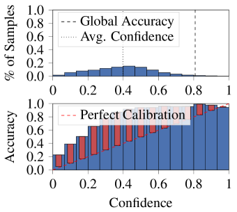
(a) ResNet-50 – original

(b) ResNet-50 – TS

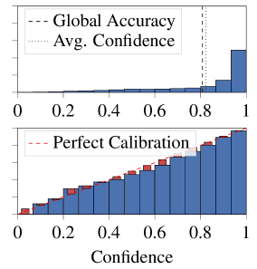
(c) ResNet-50 – TS_TvA

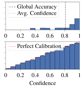
(d) ResNet-50 – HB_TvA

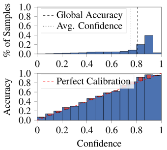
(e) ViT-B/16 – original

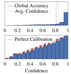
(f) ViT-B/16 – VS

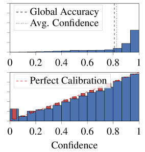
(g) ViT-B/16 – VS_{reg_TvA}

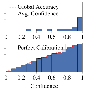
(h) ViT-B/16 – HB_TvA

Figure 1: Reliability diagrams for ResNet-50 and ViT-B/16 when using Temperature Scaling (TS), Vector Scaling (VS), and Histogram Binning (HB) on ImageNet. The subscript _TvA signifies that the TvA reformulation was used, and _reg means our regularization (6) was applied. Red bars show the differences between bin accuracy (blue bar) and accuracy for perfect calibration (dashed red line). As the methods improve the calibration, these differences are reduced and the average confidence (vertical dotted line) will get closer to the global accuracy (vertical dashed line).

5.1 Setting

Datasets and models

For image classification, we used the datasets CIFAR-10 (C10) and CIFAR-100 (C100) [27] with $10$ and $100$ classes respectively, ImageNet (IN) [7] with $1000$ classes, and ImageNet-21K (IN21K) [54] with $10450$ classes. For text classification, we used Amazon Fine Foods (AFF) [43] and DynaSent (DF) [51] for sentiment analysis with $3$ classes, MNLI [66] for natural language inference with $3$ classes, and Yahoo Answers (YA) [73] for topic classification on $10$ classes. Experiment results are averaged over five random seeds that randomly split the concatenation of the original validation and test sets into calibration and test sets.
We used the following models for image classification: ResNet [21], Wide-ResNet-26-10 (WRN) [71], DenseNet-121 [24], MobileNetV3 (MN3) [23], ViT [9], ConvNeXt [41], EfficientNet [56, 57], Swin [40, 39], and CLIP [52] which matches input images to text descriptions in a shared embedding space, assigning labels based on the highest similarity score. For text classification, we used the PLMs RoBERTa [37] and T5 [53].
More details about datasets, calibration sets sizes, and model weights can be seen in Appendix F.

Baselines

Our Top-versus-All (_TvA) reformulation and regularization (_reg) can be applied to different calibration methods. We have tested the following scaling methods: Temperature Scaling (TS) and Vector Scaling (VS) [17], and Dirichlet Calibration (DC) [29] with the best-performing variant Dir-ODIR, which regularizes off-diagonal and bias coefficients. We also tested the following binary methods: Histogram Binning (HB) [69] using for each case the best-performing variant between equal-mass or equal-size bins, Isotonic Regression (Iso) [70], Beta Calibration (Beta) [28], and Bayesian Binning into Quantiles (BBQ) [46]. For comparison, we include methods with state-of-the-art results on problems with many classes: I-Max [49] and IRM [72]. See Appendix C for more details on these methods. More details on code implementations can be seen in Appendix F.

Table 1: ECE in % (lower is better). The subscript _TvA denotes that our reformulation was applied to the calibration method. IRM and I-Max are competing methods. The best method for a given model is in bold. Methods in purple impact the model prediction, potentially degrading accuracy; methods in teal do not. Values are averaged over five random seeds. Results are averaged over models of the same family. Detailed results for all models can be seen in Tables 5 and 6 of the Appendix.

					scaling methods						binary methods
Dataset	Models	Uncal.	IRM	I-Max	TS	TSTvA	VS	VSreg_TvA	DC	DCreg_TvA	Iso	IsoTvA	BBQ	BBQTvA	HB	HBTvA
C10	ConvNets	1.77	0.67	0.61	1.20	1.25	1.17	1.17	1.16	1.17	1.12	0.68	1.17	0.77	1.06	0.43
	CLIP	5.03	1.03	0.94	0.78	0.73	2.56	1.85	2.56	1.84	1.05	0.86	1.39	0.86	1.82	0.73
C100	ConvNets	6.04	1.30	1.15	4.65	2.96	4.91	2.35	4.89	2.35	5.33	1.38	9.63	1.35	9.56	1.02
	CLIP	10.37	2.90	2.57	2.54	2.51	7.78	2.86	7.55	1.84	2.53	1.61	7.48	1.48	7.23	1.39
IN	ResNet	15.26	1.31	1.07	2.65	1.89	2.77	1.67	3.59	2.23	3.05	0.79	8.41	0.76	7.49	0.55
	EffNet	15.72	0.68	0.48	3.48	2.59	3.67	1.26	3.65	1.23	2.83	0.68	6.55	0.64	4.39	0.43
	ConvNeXt	16.46	0.82	0.58	3.67	2.25	4.05	1.37	4.04	1.35	2.97	0.75	7.41	0.68	5.13	0.52
	ViT	4.40	0.81	0.61	4.09	2.96	4.31	2.02	4.31	1.99	3.60	0.77	6.64	0.73	6.59	0.52
	Swin	5.85	0.75	0.49	3.63	2.91	4.04	1.70	4.03	1.67	3.19	0.74	7.09	0.71	5.39	0.48
	CLIP	1.96	1.08	0.72	1.89	1.82	1.63	1.05	32.03	67.65	2.35	0.92	8.31	0.93	7.16	0.80
IN21K	MN3	12.34	err.	err.	8.69	4.39	2.52	2.40	58.84	81.16	2.00	0.21	err.	0.20	5.50	0.17
	ViT-B/16	6.27	err.	err.	8.92	6.55	2.38	1.54	8.22	3.20	2.14	0.22	err.	0.24	7.89	0.12
AFF	T5	5.47	0.27	0.26	1.10	1.15	1.52	1.42	1.18	1.31	0.37	0.27	0.39	0.28	2.87	0.17
	RoBERTa	7.37	0.30	0.28	2.40	2.33	1.41	1.85	1.38	1.68	0.52	0.27	0.75	0.35	4.02	0.20
DS	T5	8.86	1.39	1.38	2.19	2.17	6.13	2.00	5.91	2.02	1.50	1.55	1.38	1.58	1.90	1.12
	RoBERTa	16.12	1.56	1.50	12.07	12.07	14.66	6.80	13.90	5.57	1.71	1.53	1.64	1.14	1.05	0.91
MNLI	T5	7.04	0.72	0.70	2.81	2.80	4.46	1.79	4.31	1.82	0.80	0.74	1.38	0.69	2.09	0.43
	RoBERTa	9.22	0.89	0.71	5.72	5.72	6.99	1.92	6.59	1.99	1.00	0.92	1.67	0.84	1.02	0.60
YA	T5	7.84	0.80	0.81	1.07	1.35	3.70	1.16	3.75	1.15	1.73	0.82	2.81	0.96	3.65	0.69
	RoBERTa	19.59	0.97	0.79	12.39	12.38	16.47	2.52	16.07	2.21	1.92	0.99	5.00	0.75	3.41	0.58

5.2 Top-versus-All

For visual qualitative results, Figure 1 displays reliability diagrams [47]. We observe that initially, ResNet-50 is highly underconfident and ViT-B/16 a bit underconfident. Applying TS and VS solves the underconfidence and makes the models slightly overconfident. TvA improves these methods, and the average confidence gets closer to the accuracy. HB_TvA makes the calibration almost perfect.

Table 1 shows the results of applying the Top-versus-All reformulation to several calibration methods. For clarity, results are averaged over families of models (models based on the same architecture) and the full results are available in Tables 5 and 6 of the Appendix. In most cases, the TvA reformulation significantly lowers the ECE by dozens of percent. Without TvA, binary methods often perturb the prediction and degrade the classifier’s accuracy (see Table 9), making them inapplicable in a practical setting. TvA solves the issue as it only scales the confidence (after the prediction is made) and makes binary methods outperform scaling methods.

Improvements due to TvA are consistent across models. However, exceptions are observed for CLIP: it is the model family with the lowest ECE pre-calibration, but the highest ECE post-calibration for ImageNet. CLIP’s multimodal training regime, zero-shot adaptation as a classifier, and very large training dataset might cause this different behavior. CLIP’s low ECE was also observed in [44, 11]. [64] specifically tackles the calibration of fine-tuned CLIP, a setting not considered here.

We also found that DC is sensitive to hyperparameter tuning, and its performance is usually not much better than VS, which is consistent with [29]. In some cases, the optimization diverges, leading to very poor results, e.g., for CLIP on ImageNet.

Improvements due to TvA are also consistent across datasets, although they tend to increase with the number of classes. Improvements on ImageNet are usually better than on CIFAR-100, whose improvements are usually better than on CIFAR-10. This is notable with e.g., TS or HB. The magnitude of improvement is usually higher for binary methods, e.g., HB, than scaling methods, e.g., TS, especially for many classes. This indicates that Issue 3 is more serious than Issue 1.

For text datasets with only three classes (AFF, DS, and MNLI), TS does not benefit from TvA, but other methods do, despite the small number of classes. According to [5], TS is among the best calibration methods for the text classification tasks considered here, even compared to ones that retrain the model. Even so, our method HB_TvA significantly outperforms it.

Some methods’ current implementations could not handle the large scale of ImageNet-21K, resulting in out-of-memory errors written as "err." in the Table. For I-Max and IRM, this is because they consider the full probability vectors while TvA efficiently uses data by considering only confidence values. Indeed, TvA handles this scale without difficulty.

Additional results are included in Appendix H. Tables 5 and 6 contain the full results for ECE, with the standard deviations in Table 7. Table 8 reveals that ImageNet networks are mostly underconfident. This is aligned with [11] and goes against previous knowledge on overconfidence, which was initially believed to be linked to network size [17]. Table 9 provides the accuracies after calibration. Table 10 exhibits that ECE with equal-mass bins has similar values as standard ECE. Table 11 shows that TvA mostly lowers the Brier score, except for Iso, which has the lowest score overall.

Calibration methods can also be applied to Large Languages Models (LLMs) using In-Context Learning (ICL) to tackle text classification tasks [77, 20, 25, 78, 1]. The primary goal of these methods is to improve model accuracy. TvA was not designed for this objective, but it can still be applied on top of an existing method that improves the accuracy. TvA then lowers the calibration error while keeping the accuracy gain. Results for GPT-J [62] and Llama-2 [59] are in Table 12.

To summarize the results for practical use, our experiments show that Histogram Binning (within the TvA or I-Max setting) is the best calibration method overall, providing ECE values mostly below 1%. This is the method we advise using. However, suppose the underlying application requires a confidence with continuous values, e.g., to rank the predictions for selective classification. In that case, we advise using a method that improves the AUROC, shown in Appendix G, such as TS or Iso.

5.3 Solving overfitting with regularization and TvA

On ImageNet, VS and DC overfit the calibration set, degrading the calibration on the test set. The lower performance of VS relative to TS indicates this overfitting. As visualized in Figure 3, combining the binary cross-entropy loss used in the TvA reformulation and an additional regularization term prevents overfitting. We fixed the value $\lambda=0.01$ as it works well across models. Initializing the vector coefficients to $\frac{1}{T}$ with $T$ obtained by TS_TvA helps further improve performance.

5.4 Influence of the calibration set size

The size of the calibration set influences the performance of the different methods, as seen in Figure 3. TS and TS_TvA do not benefit from more data due to their low expressiveness. VS does not improve the ECE because of the overfitting problem. In contrast, VS_{reg_TvA} benefits from more calibration data. With enough data ($\approx$ 15000), it outperforms TS_TvA. Binary methods using the standard One-versus-All approach have poor performance and need a large amount of data to be competitive. Using TvA, they get excellent performance with little data.

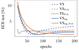
Figure 2: Test ECE evolution during training with ResNet-50 on ImageNet. The combination of regularization and TvA prevents overfitting of Vector Scaling. Temperature Scaling with TvA is shown for reference.

Figure 3: Influence of the calibration set size for ResNet-101 on ImageNet. Binary methods at the top and scaling methods at the bottom.

6 Limitations

Our approach tackles confidence calibration and is unlikely to improve performance for stronger notions of calibration, such as class-wise calibration. However, confidence calibration is useful for many practical cases, such as selective classification [13], out-of-distribution detection [22], or active learning [34]. Also, calibration improvements are less significant for problems with few classes ($\leq 10$) than for problems with many classes, but our approach still provides the best results.

7 Conclusion

Reducing the miscalibration of neural networks is essential to improve trust in their predictions. This can be done after the model training with an optimization using calibration data. However, many current calibration methods do not scale well to complex datasets: binary methods under the One-versus-All setting do not have enough per-class calibration data, and scaling methods are inefficient. We demonstrate that reformulating the confidence calibration of multiclass classifiers as a single binary problem significantly improves the performance of baseline calibration techniques. The competitiveness of scaling methods is increased, and binary methods use per-class calibration data more efficiently without altering the model’s accuracy. In short, our TvA reformulation enhances many existing calibration methods with little to no change in their algorithm. Extensive experiments with state-of-the-art image classification models on complex datasets and with text classification demonstrate our approach’s scalability and generality.

Appendix A Appendix contents

B discusses the broader impacts of the work.
C discusses the proposed approach in more details, and compares with other methods.
D contains a theoretical justification for Top-versus-All in the case of Temperature Scaling.
E discusses the limits of classwise-ECE and top-label-ECE for a high number of classes.
F describes implementation details, including the computing time in Table 3.
G shows the impact of different calibration methods on selective classification.
H provides additional results: full ECE results in Table 5 and 6, standard deviations in Table 7, confidences in Table 8, accuracies in Table 9, equal-mass bins ECE in Table 10, Brier score in Table 11, experiments for in-context learning of LLMs in Table 12.

Appendix B Broader impacts

Our reformulation of the confidence calibration of multiclass classifiers as a binary problem is both simple and general. It has several benefits. On the theoretical side, it might lead to new perspectives on the confidence calibration problem and the development of new calibration methods. On the practical side, existing calibration methods can be adapted to our problem reformulation by adding just a few lines of code. This is an easy and quick way to improve the calibration of classification models. Better-calibrated models are more trustworthy: potential incorrect predictions are more easily identifiable and preventable. However, this also comes with potential risks. The knowledge that a model is well-calibrated might lead to undue trust in the system and the tendency to overlook prediction errors. Even well-calibrated models are not entirely reliable, and developers and users must remember this. Post-processing calibration requires data not included in the training set, which leaves less data available for a thorough evaluation of the model. Calibration does not fix biases in the data. Finally, we tested the calibration improvement only on in-distribution data, but real systems might receive out-of-distribution data (e.g., an image of a new class) or adversarial examples. For such inputs, the classifier predicted probabilities (and thus the confidence) are unreliable, even for well-calibrated models, and a pipeline to filter such data is necessary.

Appendix C Details on the method

Algorithm 2 Standard approach

Input:

$D_{cal}$: $\{(x_{i},y_{i})\}_{i=1}^{N}$ the calibration data

$f$: the multiclass classifier

$g$: a calibration function $\triangleright$ e.g., Temperature Scaling

Learn calibration function:

if $g$ is scaling method then

    loss $l\coloneqq$ Cross-Entropy

    Learn $g$ to calibrate $f$ by minimizing $l$ on $D_{cal}$

else if $g$ is binary method then

    for $k=1$ to $L$ do $\triangleright$ One-versus-All approach

         $D^{k}_{cal}\leftarrow\{(x_{i},y_{i})\mid y_{i}=k\}_{i=1}^{N}$

         Learn $g_{k}$ to calibrate $f$ on $D^{k}_{cal}$

    end for

    $g\leftarrow(g_{1},g_{2},\ldots,g_{L})$

end if

Inference:

Use $g$ to calibrate confidences from $f$

Algorithm 3 Top-versus-all approach

Input:

$D_{cal}$: $\{(x_{i},y_{i})\}_{i=1}^{N}$ the calibration data

$f$: the multiclass classifier

$g$: a calibration function $\triangleright$ e.g., Temperature Scaling

Preprocessing:

$\hat{y_{i}}\leftarrow\arg\max_{k\in\mathcal{Y}}f_{k}(x_{i})$ $\triangleright$ Compute class predictions

$y^{b}_{i}\leftarrow 1_{\mathrm{\hat{y_{i}}=y_{i}}}$ $\triangleright$ Compute predictions correctness

$f^{b}\leftarrow\max_{k\in\mathcal{Y}}f_{k}$ $\triangleright$ Create surrogate binary classifier

$D^{\text{\tiny TvA}}_{cal}\leftarrow\{(x_{i},y^{b}_{i})\}_{i=1}^{N}$ $\triangleright$ Build binary calib. set

Learn calibration function:

if $g$ is scaling method then

    loss $l\coloneqq$ Binary Cross-Entropy

    if $g$ is vector or Dirichlet scaling

     loss $l\leftarrow l+\lambda l_{reg}$ $\triangleright$ Add regularization

    end if

    Learn $g$ to calibrate $f^{b}$ by minimizing $l$ on $D^{\text{\tiny TvA}}_{cal}$

else if $g$ is binary method then

    Learn $g$ to calibrate $f^{b}$ on $D^{\text{\tiny TvA}}_{cal}$

end if

Inference:

Use $g$ to calibrate confidences from $f$

Comparison with the standard approach

Algorithm 2 describes the standard approach to post-processing calibration, and Algorithm 3 describes our approach in more details and shows in blue the differences with the standard approach. Our approach adds a preprocessing step to keep only the confidences instead of the full probabilities vector. It can be seen as creating a surrogate "correctness" classifier and its associated calibration data. The calibrator is learned for the surrogate classifier and applied to the original classifier at inference time. Also, we add regularization for some scaling methods and we have only one binary calibrator instead of one per class.

Comparison with IRM and I-Max

IRM [72] and I-Max [49] are, like TvA, multiclass-to-binary reductions. This is why TvA cannot be applied on top of them: they already transform the multiclass problem into a binary one using a different strategy.

The shared class-wise strategy of [49] and the data ensemble strategy of [72] are described very briefly in subsections 3.2 and 3.3.2 of their respective papers and not rigorously justified. Our understanding is that these two strategies do exactly the same thing. To build the calibration set, they concatenate all the class probability vectors so that we get a big probability vector of size $N.L$ ($N$ samples and $L$ classes) as predictions and similarly concatenate the one-hot embedding of the target class (a big vector with $N$ ones and $N.(L-1)$ zeros) as targets. Then, they learn a single calibrator. For each example, this calibrator aims to simultaneously increase the probabilities for the target class (target is $1$) and decrease all the other class probabilities (target is $0$). The single calibrator is applied to each class probability separately, meaning that the ranking of class probabilities can change, modifying the classifier prediction.

Our strategy derives from transforming the multiclass calibration into a single binary problem. The intuition is to learn the calibrator on a surrogate binary classifier and apply this calibrator to the original classifier. This binary classifier is built on top of the original classifier (by applying the max function to the class probabilities vector). They thus share their confidence. However, the binary classifier aims to solve a different task: predicting the correctness of the original classifier. To build the calibration set, we concatenate all the confidences (a vector of size N) as predictions and concatenate all the correctnesses as targets (also a vector of size N). The correctness value of a given example is $1$ if the class prediction is correct; otherwise, it is $0$. Then, we learn a single calibrator, similar to the strategy above. However, there is a key difference: this calibrator aims to increase the probabilities for correct predictions and decrease them for incorrect predictions. Note that our probabilities are all confidences (the maximum class probabilities), meaning we only consider the confidences, which the calibrator directly increases or decreases. In the strategy from [49] and [72], the calibrator has to manage all class probabilities (L times more), even the ones that do not matter, including the lowest class probabilities close to 0. This is less efficient (actually, while this can surely be fixed, the original implementations of IRM and I-Max could not run on ImageNet-21K). This point is closely linked to the analysis of the binary cross entropy loss for scaling methods in Subsection 4.2: when the prediction is incorrect, increasing the probability of the correct class indirectly decreases the confidence (strategy from [49] and [72]) while our strategy directly decreases the confidence.

I-Max is more complex because it modifies the Histogram Binning algorithm, while our approach does not. Additionally, [35] found that I-Max produces unusable probability vectors. Indeed, they do not sum up to $1$, and normalizing them degrades the method’s performance.

We wrote our paper with practicality and generality in mind. Contrary to [49] and [72], we demonstrate the generality of our strategy by applying it on top of existing calibration baselines of different natures (scaling and binary). One of our main goals is that practitioners can easily and quickly try our TvA approach, using just a few lines of code, which can significantly improve the calibration performance of their existing calibration pipeline while having no impact on the predicted class by design (except for VS and DC).

Comparison with ProCal

Another recent calibration method is ProCal [68]. However, its primary objective differs from ours: it "focuses on the problem of proximity bias in model calibration, a phenomenon wherein deep models tend to be more overconfident on data of low proximity". Its goal is to lower the difference in the confidence score values between regions of low and high density, i.e., to make the confidence score independent of a local density indicator called "proximity." There is no theoretical guarantee, however, that minimizing the proximity bias improves the confidence calibration, the focus of our work. Theorem 4.2 about the PIECE metric is a direct consequence of Jensen’s inequality and is true for any random variable D, not necessarily a proximity score. Theorem 5.1 is an interesting bias/variance decomposition of the Brier score. However, as this type of decomposition usually states, the error may come from bias (here, a wrong initial calibration) or high estimation variance (which can be related to low density but is not expressed as such in the decomposition). We experimentally compare our approach to the ProCal algorithm using the code provided by its authors and observe in Table 2 that our approach gives much better ECE confidence calibration and, for half of the models, also better PIECE values.

ProCal aims to achieve three goals: mitigate proximity bias, improve confidence calibration, and provide a plug-and-play method. We share the last two goals. Concerning improving confidence calibration, our approach has better results, as shown in Table 2. Both approaches are plug-and-play, but they apply very differently. ProCal is applied after existing calibration methods to further improve calibration. It thus does not solve any of the four issues we identified (e.g., cross-entropy loss is still inefficient, and One-versus-All still leads to highly imbalanced problems). Our Top-versus-All approach is a reformulation of the calibration problem that uses a surrogate binary classifier. Existing approaches are applied to this surrogate classifier, which is how the four issues are solved. We do not propose a new method but a new way of applying existing methods. Our approach does not introduce new hyperparameters (except in the particular case of regularizing scaling methods). ProCal introduces several new hyperparameters, such as the choice of the distance, the number of KNN neighbors, or a shrinkage coefficient.

Comparison with Correctness-Aware Loss

A concurrent work [38] builds a calibration method on top of an intuition similar to ours: binarize the calibration problem. However, what the authors do with this intuition differs vastly from our approach. They derive a Correctness-Aware Loss (Eq. 7 of their paper), which is almost the standard binary cross-entropy loss we use for scaling methods but without a logarithm. They use this loss to learn a separate model that predicts a sample-wise temperature coefficient. This is a new calibration method, which is not straightforward to implement due to the numerous hyperparameters (network architecture, image transformations…). It also requires multiple inferences at test-time, which can be problematic in some production models. Our approach is, again, not a calibration method but a general reformulation of the calibration problem that enhances existing methods. By looking at their Table 1, they get an ECE of 2.22 on ImageNet (in-distribution), while our approach achieves values around 0.5 for most models in our paper’s Table 1. Their method, contrary to TvA, improves the AUROC, but in our understanding, it seems mostly due to the use of image transformations, not from their proposed loss. Their method seems to work best in out-of-distribution scenarios, which is not the main objective of our paper. However, these good results for AUROC and out-of-distribution scenarios make this method complementary to our approach, and combining the two in some way could be promising.

Table 2: ECE, MCE, ACE, and PIECE in %. The experimental setting is the one used for Table 4 of [68]. The baselines are no calibration (conf), Temperature Scaling (TS), Multi Isotonic Regression (MIR), and Histogram Binning (HB). The ProCal calibration method [68] is applied after one of the baselines, as symbolized by the "+" symbol. Our approach, Top-versus-All, changes what the baselines optimize and is symbolized by "_TvA". We apply it for TS, Isotonic Regression (Iso), and HB. The best values for each model and metric are in bold.
Overall, HB_TvA is the best calibration method as it always gets the lowest ECE and ACE. Our TvA approach lowers PIECE and even achieves the lowest value for half of the models.

Model	Method	ECE ($\downarrow$)	MCE ($\downarrow$)	ACE ($\downarrow$)	PIECE ($\downarrow$)
BeiT	conf	3.60	1.52	3.58	4.26
	TS	2.99	0.76	3.08	3.56
	MIR	0.59	0.14	0.64	1.88
	HB	4.96	1.83	6.13	7.20
	conf+ProCal	1.02	0.33	0.94	1.69
	TS+ProCal	1.52	0.76	1.45	2.05
	MIR+ProCal	0.61	0.15	0.71	1.41
	HB+ProCal	5.53	4.13	5.81	6.39
	TSTvA	2.10	0.49	2.20	2.88
	IsoTvA	0.65	0.14	0.68	1.92
	HBTvA	0.44	0.19	0.58	1.70
Mixer	conf	10.78	5.00	10.78	10.86
	TS	4.81	1.92	4.72	5.57
	MIR	1.14	0.25	1.29	3.41
	HB	9.65	4.00	9.97	13.09
	conf+ProCal	2.64	0.94	2.55	3.23
	TS+ProCal	1.32	0.38	1.22	2.13
	MIR+ProCal	0.83	0.14	0.88	2.08
	HB+ProCal	6.57	4.43	7.32	7.83
	TSTvA	2.51	0.74	2.50	4.32
	IsoTvA	0.86	0.15	0.86	3.18
	HBTvA	0.64	0.19	0.75	3.17
ResNet50	conf	8.59	4.58	8.50	8.74
	TS	5.03	2.48	5.01	5.34
	MIR	0.75	0.18	0.82	1.79
	HB	7.63	2.61	9.32	10.17
	conf+ProCal	2.63	1.31	2.61	3.26
	TS+ProCal	1.66	0.66	1.53	2.50
	MIR+ProCal	0.76	0.17	0.74	1.78
	HB+ProCal	6.32	4.38	7.52	7.65
	TSTvA	6.89	1.17	6.95	7.13
	IsoTvA	0.76	0.19	0.73	1.79
	HBTvA	0.55	0.21	0.59	1.35
ViT	conf	1.14	0.33	1.09	1.83
	TS	1.46	0.46	1.41	2.03
	MIR	0.64	0.13	0.75	1.54
	HB	4.59	2.32	7.07	7.20
	conf+ProCal	0.81	0.22	0.81	1.71
	TS+ProCal	0.83	0.25	0.84	1.74
	MIR+ProCal	0.78	0.14	0.76	1.59
	HB+ProCal	6.80	4.72	7.42	7.55
	TSTvA	1.08	0.25	1.05	1.86
	IsoTvA	0.51	0.11	0.62	1.46
	HBTvA	0.37	0.17	0.51	1.20

Appendix D Theoretical justification for Top-versus-All in the case of Temperature Scaling

We define $L$ the number of classes, $f_{k}(x)$ the classifier estimated probability for class $k$ and data sample $x$, $y$ the correct class, and the confidence $s(x)\coloneqq\max_{k}f_{k}(x)$. The cross-entropy loss is $l_{CE}(x,y)=-\sum_{k=1}^{L}1\{k=y\}\cdot\log(f_{k}(x))=-\log(f_{y}(x))$. Because the last layer of the classifier is a softmax function, $f_{y}(x)=\frac{e^{z_{y}}}{\sum_{k}e^{z_{k}}}$ with $z$ the logits vector. Note that we omit the writing variable $x$ in the following for clarity.

Temperature scaling optimizes a coefficient $T>0$ that scales the logits vector. Predicted probabilities become $f_{y}(x)=\frac{e^{z_{y}/T}}{\sum_{k}e^{z_{k}/T}}$.

Let us first develop the standard cross-entropy loss when temperature scaling is applied:

$$l_{CE}=-\log(f_{y})=-\log(\frac{e^{z_{y}/T}}{\sum_{k}e^{z_{k}/T}})=-\left(\log(e^{z_{y}/T})-\log(\sum_{k}e^{z_{k}/T})\right)=-\frac{z_{y}}{T}+\log(\sum_{k}e^{z_{k}/T})$$

Let us compute its gradient:

$$\frac{\partial l_{CE}}{\partial T} =\frac{z_{y}}{T^{2}}+\frac{\partial\log(\sum_{k}e^{z_{k}/T})}{\partial\sum_{k}e^{z_{k}/T}}\cdot\frac{\partial\sum_{k}e^{z_{k}/T}}{\partial T}\text{by application of the chain rule on the second term.}$$

$$=\frac{z_{y}}{T^{2}}+\frac{1}{\sum_{k}e^{z_{k}/T}}\cdot\sum_{k}\frac{\partial e^{z_{k}/T}}{\partial T}$$

$$=\frac{z_{y}}{T^{2}}+\frac{1}{\sum_{k}e^{z_{k}/T}}\cdot\sum_{k}\frac{\partial(e^{z_{k}})^{1/T}}{\partial T}$$

$$=\frac{z_{y}}{T^{2}}+\frac{1}{\sum_{k}e^{z_{k}/T}}\cdot\sum_{k}\frac{\log(e^{z_{k}})}{-T^{2}}(e^{z_{k}})^{1/T}$$

$$=\frac{z_{y}}{T^{2}}+\frac{1}{\sum_{k}e^{z_{k}/T}}\cdot\sum_{k}\frac{z_{k}\cdot e^{z_{k}/T}}{-T^{2}}$$

$$=\frac{1}{T^{2}}\left(z_{y}-\frac{\sum_{k}z_{k}\cdot e^{z_{k}/T}}{\sum_{k}e^{z_{k}/T}}\right)$$

$$=\frac{1}{T^{2}}\left(z_{y}-\sum_{k}\frac{z_{k}\cdot e^{z_{k}/T}}{\sum_{j}e^{z_{j}/T}}\right)$$

$$=\frac{1}{T^{2}}\left(z_{y}-\sum_{k}z_{k}\cdot f_{k}\right)$$ (7)

For our TvA approach, the problem becomes binary. The classification output becomes the confidence $s(x)=\max_{j\in\mathcal{Y}}f_{j}(x)$ and the ground truth label becomes a binary representation of the prediction correctness: $y^{b}=1_{\mathrm{\hat{y}=y}}$ with $\hat{y}(x)=\arg\max_{k\in\mathcal{Y}}f_{k}(x)$ and $1$ the indicator function. The loss we use is the binary cross entropy $l_{BCE}(x,y)=-\big{(}y^{b}\cdot\log s(x)+(1-y^{b})\cdot\log(1-s(x))\big{)}$

Let us compute the gradient:

$$\frac{\partial l_{BCE}}{\partial T} =\frac{\partial l_{BCE}}{\partial s}\cdot\frac{\partial s}{\partial T}$$

$$=-\left(y^{b}\frac{1}{s}+(1-y^{b})\frac{-1}{1-s}\right)\cdot\frac{\partial s}{\partial T}$$

$$=-\left(\frac{y^{b}(1-s)}{s(1-s)}-\frac{s(1-y^{b})}{s(1-s)}\right)\cdot\frac{\partial s}{\partial T}$$

$$=\frac{s-y^{b}}{s(1-s)}\cdot\frac{\partial s}{\partial T}$$

$$=\frac{s-y^{b}}{s(1-s)}\cdot\frac{\partial\frac{e^{z_{m}/T}}{\sum_{k}e^{z_{k}/T}}}{\partial T}\text{ because }s=\max_{j}\frac{e^{z_{j}/T}}{\sum_{k}e^{z_{k}/T}}=\frac{e^{z_{m}/T}}{\sum_{k}e^{z_{k}/T}}\text{ with }z_{m}=\max_{k}z_{k}$$

$$=\frac{s-y^{b}}{s(1-s)}\cdot\frac{\frac{\partial e^{z_{m}/T}}{\partial T}\sum_{k}e^{z_{k}/T}-e^{z_{m}/T}\frac{\partial\sum_{k}e^{z_{k}/T}}{\partial T}}{(\sum_{k}e^{z_{k}/T})^{2}}$$

$$=\frac{s-y^{b}}{s(1-s)}\cdot\frac{\frac{\log(e^{z_{m}})}{-T^{2}}(e^{z_{m}})^{1/T}\sum_{k}e^{z_{k}/T}-e^{z_{m}/T}\sum_{k}\frac{\log(e^{z_{k}})}{-T^{2}}(e^{z_{k}})^{1/T}}{(\sum_{k}e^{z_{k}/T})^{2}}$$

$$=\frac{s-y^{b}}{s(1-s)}\cdot\frac{e^{z_{m}/T}}{T^{2}}\cdot\frac{-\log(e^{z_{m}})\sum_{k}e^{z_{k}/T}+\sum_{k}\log(e^{z_{k}})(e^{z_{k}})^{1/T}}{(\sum_{k}e^{z_{k}/T})^{2}}$$

$$=\frac{s-y^{b}}{s(1-s)}\cdot\frac{e^{z_{m}/T}}{T^{2}}\cdot\frac{-z_{m}\sum_{k}e^{z_{k}/T}+\sum_{k}z_{k}\cdot e^{z_{k}/T}}{(\sum_{k}e^{z_{k}/T})^{2}}$$

$$=\frac{s-y^{b}}{s(1-s)}\cdot\frac{1}{T^{2}}\cdot s\cdot\frac{-z_{m}\sum_{k}e^{z_{k}/T}+\sum_{k}z_{k}\cdot e^{z_{k}/T}}{\sum_{k}e^{z_{k}/T}}$$

$$=\frac{1}{T^{2}}\cdot\frac{s-y^{b}}{1-s}\cdot\frac{-z_{m}\sum_{k}e^{z_{k}/T}+\sum_{k}z_{k}\cdot e^{z_{k}/T}}{\sum_{k}e^{z_{k}/T}}$$

$$=\frac{1}{T^{2}}\cdot\frac{s-y^{b}}{1-s}\cdot\left(\frac{\sum_{k}z_{k}\cdot e^{z_{k}/T}}{\sum_{k}e^{z_{k}/T}}-z_{m}\right)$$

$$=\frac{1}{T^{2}}\cdot\frac{y^{b}-s}{1-s}\cdot\left(z_{m}-\frac{\sum_{k}z_{k}\cdot e^{z_{k}/T}}{\sum_{k}e^{z_{k}/T}}\right)$$

$$=\frac{1}{T^{2}}\cdot\frac{y^{b}-s}{1-s}\cdot\left(z_{m}-\sum_{k}\frac{z_{k}\cdot e^{z_{k}/T}}{\sum_{j}e^{z_{j}/T}}\right)$$

$$=\frac{1}{T^{2}}\cdot\frac{y^{b}-s}{1-s}\cdot\left(z_{m}-\sum_{k}z_{k}\cdot f_{k}\right)$$ (8)

- First case, the prediction is correct: $y^{b}=1$ and $z_{m}=z_{y}$. Let us inject these in (8): $\frac{\partial l_{BCE}}{\partial T}=\frac{1}{T^{2}}\cdot\left(z_{y}-\sum_{k}z_{k}\cdot f_{k}\right)=\frac{\partial l_{CE}}{\partial T}$. We thus get the same gradient as the standard cross-entropy loss.

- Second case, the prediction is incorrect: $y^{b}=0$ and $z_{m}>z_{y}$. (8) becomes: $\frac{\partial l_{BCE}}{\partial T}=\frac{1}{T^{2}}\cdot\frac{s}{s-1}\cdot\left(z_{m}-\sum_{k}z_{k}\cdot f_{k}\right)$. By comparing to (7), we have the term $\frac{1}{T^{2}}\cdot\left(z_{m}-\sum_{k}z_{k}\cdot f_{k}\right)>\frac{1}{T^{2}}\left(z_{y}-\sum_{k}z_{k}\cdot f_{k}\right)=\frac{\partial l_{CE}}{\partial T}$ and the remaining part of (8) $|\frac{s}{s-1}|>1\text{ when }s>0.5$.
So to recapitulate, $|\frac{\partial l_{BCE}}{\partial T}|>|\frac{\partial l_{CE}}{\partial T}|$ when $s>0.5$, which corresponds to the vast majority of data points as the classifier gets better calibrated. This is shown in Figure 1.
We also have $\lim_{{s\to 1}}|\frac{s}{s-1}|=\infty$. In practice, $s$ is not close enough to $1$ to generate exploding gradients, so it just means that as confidences for wrong predictions gets higher, so does the gradient to reduce the confidences.

The conclusion is that for correct predictions, our approach does not change the optimization, but for incorrect predictions, the gradient is stronger and penalizes more heavily confident predictions that are wrong. This is also proven experimentally by looking at Table 8 where we see that average confidences of temperature scaling with the TvA approach (TS_TvA) are lower than the ones using the standard approach (TS), for almost all networks. This makes the average confidences closer to the accuracy, showing reduced overconfidence.

Appendix E Limits of classwise-ECE and top-label-ECE for a high number of classes

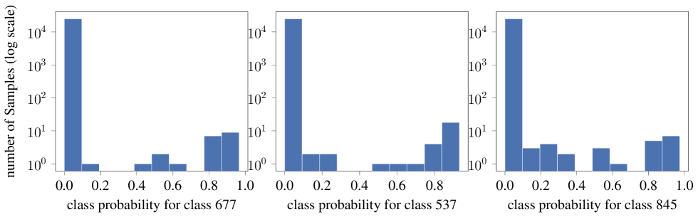
Figure 4: Histogram of class probabilities for 3 random classes, for ViT-16/B on ImageNet.

Let us define the ECE for class $j$:

$$\text{ECE}_{j}=\sum_{b=1}^{B}\frac{n_{b}}{N}|\text{acc}(b,j)-\text{conf}(b,j)|$$

The difference compared to (2) is that now $\text{acc}(b,j)$ corresponds to the proportion of class $j$ in the bin. Also, $\text{conf}(b,j)$ now is the average probability given to class $j$ for all samples in the bin.
Then, classwise-ECE [29] takes the average for all classes:

$$\text{ECE}_{\text{cw}}=\sum_{j=1}^{L}\text{ECE}_{j}$$

Classwise-ECE considers the full probabilities vectors: all the class probabilities for each prediction. However, this metric does not scale to large numbers of classes. Let us see why with an example.

Let us use a test set of $N$ samples, $N/L$ for each of the $L$ classes (the dataset is balanced), and a high-accuracy classifier fairly calibrated. The classifier predicts $N$ probability vectors of length $L$. Predicted probabilities for class $j$ are all the values of the vector at dimension $j$. Because the classifier has a high accuracy and is fairly calibrated, around $N/L$ values are close to $1$ (corresponding to mostly correct predictions), and the remaining ones, around $N-N/L$, are close to $0$ (because the predicted class is not class $j$, and the predicted probability is high for another class).

To compute $\text{ECE}_{j}$ with equal size 15 bins, the predicted probabilities for class $j$ are partitioned into 15 bins. The first bin (with probabilities close to 0), contains $n_{1}\approx N-N/L$ samples while the last one (with probabilities close to 1) contains $n_{B}\approx N/L$ samples. The remaining bins are usually even more empty. That means that the calibration error in the first bin is weighted $n_{1}/n_{B}=L-1$ times more than the last one. For the 1000 classes of ImageNet, $L-1=999$. Figure 4 shows the number of samples ($n_{b}$) in each bin for an ImageNet classifier.

Because the impact of the calibration error in the bin with the high probabilities is negligible relative to the bin with the low probabilities, the classwise-ECE mostly measures whether probabilities close to 0 are calibrated. We argue this is not what we are interested in: what matters more is the calibration of higher values of the probabilities.

Top-label ECE [18] is another interesting metric that does not scale to large numbers of classes either. Top-label-ECE divides data into subsets according to the predicted class, computes the ECEs of these subsets, and averages them. For an ImageNet test set of 25000 samples (25 per class), data is divided into 1000 subsets of $\approx$ 25 samples each (the classifier is high-accuracy, most of the time the predicted class is equal to the true class). The ECE is computed for each subset containing only 25 samples. To compute the ECE, samples are typically partitioned into 15 bins. The number of samples per bin does not allow a correct estimation of the average confidence or accuracy.

Appendix F Implementation details

F.1 Models weights

• Model weights for CIFAR are from [45].

• Model weights for ImageNet come from torchvision [42].

• Model weights for ImageNet-21K are from [54].

• CLIP weights are from OpenAI’s Hugging Face.

• Original weights for T5 and RoBERTa come from the Transformers library [67]. The models are fine-tuned for each task using prompt-based learning [36]. For more details, see [5].

• We used the model GPT-J https://huggingface.co/EleutherAI/gpt-j-6b (Apache-2.0 license) and Llama-2 https://huggingface.co/meta-llama/Llama-2-13b (license).

F.2 Datasets

• CIFAR-10 (C10) and CIFAR-100 (C100) [27] contain 60000 32x32 images corresponding to 10 and 100 classes, respectively. Data is split into subsets of 45000/5000/10000 images for train/validation/test. We concatenate the original validation and test sets, and randomly split that into a calibration set of size 5000, and a test set of size 10000.

• ImageNet (IN) [7] contains 1.3 million images from 1000 classes. Following [17], we randomly split the original validation test of size 50000 into a calibration set and a test set, both of size 25000.

• ImageNet-21K (IN21K) [54], in its winter21 version, contains 11 million images in the train set, and 522500 in the test set (50 for each of the 10450 classes). We randomly split the test set into equal-sized calibration and test set (261250 samples each, 25 per class).

• Amazon Fine Foods [43] is a collection of customer reviews for fine foods sold on Amazon. Reviews are categorized into bad, neutral, and good. The original validation set size is 78741 and test size 91606. We randomly split them into 78741 samples for calibration and 91606 for test.

• DynaSent [51] is a dynamic benchmark for sentiment analysis consisting of sentences annotated as positive, neutral, and negative. The original validation set size is 11160 and test size 4320. We randomly split them into 11160 samples for calibration and 4320 for test.

• MNLI [66] contains pairs of sentences labeled as contradiction, neutral, and entailment. The original validation set size is 19635 and test size 9815. We randomly split them into 19635 samples for calibration and 9815 for test.

• Yahoo Answers (YA) [73] contains question-answers pairs corresponding to 10 different topics. The original validation set size is 14000 and test size 60000. We randomly split them into 14000 samples for calibration and 60000 for test.

• TREC [61] contains questions categorized into 6 classes. The training set contains 5500 labeled questions, and the test set contains another 500.

• SST-5 [55] contains 11855 sentences corresponding to 5 sentiments (from very negative to very positive).

• DBpedia [74] contains text for topic classification with 14 classes. The training set contains 560000 samples, and the test set 5000.

F.3 Code

• We used the library netcal [32] (Apache-2.0 license) for their implementation of binary methods for calibration and adapted their reliability diagrams code. For HB, we tested equal-size and equal-mass bins, and chose the best variant for each case. All hyperparameters were kept at their default values (10 bins for HB).

• We took inspiration from the official implementation of temperature scaling: https://github.com/gpleiss/temperature_scaling (MIT license).

• We took inspiration from the official implementation of Dirichlet calibration: https://github.com/dirichletcal/experiments_dnn (MIT license).

• We used the official implementation of I-Max: https://github.com/boschresearch/imax-calibration (AGPL-3.0 license).

• We used the official implementation of IRM: https://github.com/zhang64-llnl/Mix-n-Match-Calibration (MIT license).

• For evaluation, we used codes from https://github.com/JeremyNixon/uncertainty-metrics-1 (Apache-2.0 license) and https://github.com/IdoGalil/benchmarking-uncertainty-estimation-performance (MIT license).

• We used PyTorch 2.0.0 [3] (BSD-style license).

• We used CIFAR models from [45] https://github.com/torrvision/focal_calibration (MIT license).

• We used ImageNet-21K models [54] https://github.com/Alibaba-MIIL/ImageNet21K (MIT license).

• We used CLIP models from HuggingFace’s Transformers library [67] (Apache-2.0 license).

• We used pretrained language models from Transformers [67] and calibration codes from [5] https://github.com/lifan-yuan/PLMCalibration (MIT license).

• We used code from https://github.com/mominabbass/LinC for the calibration of LLMs using ICL, itself built upon https://github.com/tonyzhaozh/few-shot-learning (Apache-2.0 license).

Table 3: Computing time (in seconds) of the calibration on ImageNet, using one NVIDIA V100 GPU. The first column denotes the data preprocessing time, which includes computing the model logits for all calibration examples. Post-hoc calibration methods do not usually require much computing power compared to classifier training.

Model	Preproc.	IRM	I-Max	TS	TSTvA	VS	VSreg_TvA	DC	DCreg_TvA	HB	HBTvA	Iso	IsoTvA	Beta	BetaTvA	BBQ	BBQTvA
ResNet-50	141	2021	543	215	218	214	217	226	226	129	1	66	1	873	22	1156	2
ViT-B/16	151	7119	524	225	226	217	222	232	235	127	1	61	1	917	23	1169	2

Appendix G Impact on selective classification

Table 4: AUROC in % (higher is better). Methods in purple impact the model prediction, potentially degrading accuracy; methods in teal do not. Improvements from the uncalibrated model are colored in blue and degradations in orange.

(a) CIFAR-10

Model	Uncal.	IRM	I-Max	TS	TSTvA	VS	VSreg_TvA	DC	DCreg_TvA	Beta	BetaTvA	Iso	IsoTvA	BBQ	BBQTvA	HB	HBTvA
ResNet-50	92.09	91.79	91.30	92.01	91.98	92.71	92.76	92.71	92.76	90.94	92.09	92.29	91.87	75.63	85.53	75.78	84.69
ResNet-110	92.26	92.25	91.53	92.19	92.18	92.18	92.31	92.16	92.30	91.33	92.26	92.40	92.20	73.44	85.01	74.46	84.56
WRN	91.17	91.17	90.36	91.21	91.19	91.80	92.32	91.82	92.31	90.45	91.17	92.28	91.18	75.99	86.62	73.91	85.38
DenseNet	90.46	90.15	89.68	90.48	90.45	90.84	91.40	90.84	91.39	89.98	90.46	91.46	90.12	77.07	87.07	74.61	83.07
CLIP (ViT-B/32)	89.85	89.72	89.73	89.97	89.97	90.73	91.07	90.95	91.14	90.58	89.85	90.28	89.66	88.86	89.41	88.01	88.76
CLIP (ViT-B/16)	91.00	90.96	90.72	91.10	91.10	91.79	91.99	91.88	92.06	91.75	91.00	90.69	90.83	89.36	90.57	89.12	89.97
CLIP (ViT-L/14)	93.22	93.15	94.32	93.32	93.31	93.69	93.78	93.79	93.87	93.17	93.22	92.78	93.05	87.29	91.73	88.65	91.33

(b) CIFAR-100

Model	Uncal.	IRM	I-Max	TS	TSTvA	VS	VSreg_TvA	DC	DCreg_TvA	Beta	BetaTvA	Iso	IsoTvA	BBQ	BBQTvA	HB	HBTvA
ResNet-50	85.80	85.78	85.03	85.73	85.62	85.92	86.50	85.91	86.51	85.49	85.80	87.19	85.69	81.21	85.31	81.90	83.90
ResNet-110	85.03	84.99	83.76	84.94	84.85	84.82	85.34	84.84	85.33	84.57	85.03	86.32	84.97	80.54	84.47	81.40	82.93
WRN	87.59	87.52	87.02	87.59	87.48	87.83	88.17	87.85	88.14	87.45	87.59	88.65	87.46	83.59	86.46	83.77	85.69
DenseNet	86.17	86.02	85.64	86.12	86.00	86.60	86.79	86.59	86.79	86.01	86.17	87.09	86.11	83.02	85.42	83.47	84.86
CLIP (ViT-B/32)	83.06	83.14	82.99	83.74	83.70	83.95	85.16	83.99	85.02	84.17	83.06	84.61	82.95	85.59	83.00	85.61	82.82
CLIP (ViT-B/16)	82.57	82.55	82.51	83.65	83.66	83.95	85.29	84.04	85.76	84.18	82.57	84.45	82.51	85.76	82.46	85.62	82.24
CLIP (ViT-L/14)	84.26	84.22	84.14	85.51	85.50	86.56	87.57	86.62	87.50	85.64	84.26	86.94	84.11	86.92	84.12	86.67	84.07

(c) ImageNet

Model	Uncal.	IRM	I-Max	TS	TSTvA	VS	VSreg_TvA	DC	DCreg_TvA	Beta	BetaTvA	Iso	IsoTvA	BBQ	BBQTvA	HB	HBTvA
ResNet-18	85.73	85.70	85.37	85.64	85.65	85.63	85.88	85.30	85.39	84.39	85.73	86.12	85.69	83.19	85.40	83.73	85.03
ResNet-34	86.18	86.19	85.78	86.11	86.10	86.25	86.38	85.86	85.99	84.64	86.18	86.41	86.14	82.26	85.77	83.03	85.77
ResNet-50	80.53	80.54	80.12	85.93	85.69	85.60	85.57	85.58	85.57	82.34	80.53	86.91	80.49	85.27	80.52	83.63	79.96
ResNet-101	84.18	84.20	83.57	85.96	85.71	85.38	85.56	85.34	85.53	82.38	84.18	87.09	84.18	82.48	84.11	81.16	83.80
EffNet-B7	84.92	84.84	84.10	86.61	86.34	85.18	85.51	85.18	85.52	81.91	84.92	87.14	84.87	81.57	84.94	80.38	84.26
EffNetV2-S	85.77	85.87	85.29	87.02	86.86	85.30	85.67	85.28	85.68	82.55	85.77	87.42	85.72	82.44	85.75	80.86	84.80
EffNetV2-M	82.36	82.36	81.58	85.26	84.92	83.66	84.19	83.64	84.23	80.51	82.36	86.51	82.32	81.24	82.23	79.45	81.71
EffNetV2-L	84.63	84.58	83.96	86.33	86.05	85.77	85.94	85.75	85.87	82.27	84.63	86.70	84.55	81.78	84.56	80.56	84.08
ConvNeXt-T	82.35	82.31	81.84	85.47	85.18	85.60	85.57	85.59	85.59	81.93	82.35	86.97	82.29	82.58	82.30	81.44	81.88
ConvNeXt-S	82.29	82.36	81.87	85.27	84.88	84.81	85.01	84.81	85.01	81.22	82.29	86.98	82.26	81.29	82.20	79.78	81.86
ConvNeXt-B	82.27	82.27	81.70	85.13	84.75	84.40	84.88	84.40	84.90	80.87	82.27	87.01	82.22	81.79	82.25	79.89	81.69
ConvNeXt-L	82.35	82.35	81.42	84.81	84.38	84.04	84.58	84.04	84.54	80.24	82.35	86.79	82.32	80.49	82.23	79.15	81.75
ViT-B/32	85.57	85.60	85.10	86.31	86.13	85.95	85.98	85.93	85.98	83.56	85.57	87.16	85.54	83.39	85.55	82.69	85.11
ViT-B/16	85.52	85.55	84.92	86.32	86.12	85.36	85.53	85.34	85.56	81.82	85.52	87.19	85.50	81.56	85.39	81.21	85.09
ViT-L/32	85.42	85.45	84.78	85.93	85.73	85.19	85.29	85.20	85.30	82.07	85.42	87.25	85.41	81.51	85.40	81.42	85.09
ViT-L/16	85.85	85.83	84.63	86.16	86.00	84.33	84.65	84.32	84.64	80.96	85.85	86.97	85.83	79.76	85.66	80.08	84.85
ViT-H/14	87.28	87.24	86.60	87.53	87.34	86.74	86.71	86.77	86.78	82.15	87.28	86.65	87.22	79.33	86.54	80.08	85.32
Swin-T	85.68	85.71	85.04	86.50	86.34	85.79	85.86	85.80	85.86	83.14	85.68	87.10	85.66	82.15	85.64	81.39	85.16
Swin-S	85.37	85.36	84.75	85.99	85.78	84.99	85.20	85.00	85.20	80.92	85.37	86.92	85.35	80.25	85.32	80.05	84.80
Swin-B	84.11	84.26	83.38	85.26	84.91	83.93	84.18	83.92	84.20	79.78	84.11	86.55	84.19	78.94	84.24	79.09	83.09
SwinV2-T	85.80	85.79	85.10	86.74	86.56	85.82	86.04	85.80	86.02	83.06	85.80	87.29	85.78	82.58	85.76	81.47	85.26
SwinV2-S	85.75	85.75	85.03	86.61	86.39	85.19	85.51	85.19	85.50	81.77	85.75	87.18	85.74	80.54	85.75	80.41	84.73
SwinV2-B	85.15	85.13	84.19	86.07	85.82	84.43	84.70	84.40	84.65	80.31	85.15	86.99	85.16	79.57	84.98	79.42	83.86
CLIP (ViT-B/32)	80.56	80.56	80.24	80.59	80.57	81.73	83.21	77.72	77.92	81.14	80.56	81.43	80.52	81.85	80.53	82.14	80.18
CLIP (ViT-B/16)	81.12	81.08	80.96	81.16	81.15	82.28	83.64	78.10	84.57	81.52	81.12	82.17	81.10	82.33	81.07	82.42	80.76
CLIP (ViT-L/14)	82.98	82.95	82.50	82.90	82.86	83.66	85.07	80.09	79.86	82.75	82.98	83.29	82.93	82.85	82.80	82.87	82.36

(d) ImageNet-21K

Model	Uncal.	IRM	I-Max	TS	TSTvA	VS	VSreg_TvA	DC	DCreg_TvA	Beta	BetaTvA	Iso	IsoTvA	BBQ	BBQTvA	HB	HBTvA
MN3	68.79	err.	err.	67.80	65.89	80.00	81.00	61.24	51.94	err.	68.79	79.62	68.77	err.	68.77	90.86	68.40
ViT-B/16	72.99	err.	err.	74.36	73.17	79.78	81.42	76.29	78.92	err.	72.99	79.66	73.10	err.	73.20	90.27	71.95

(e) Amazon Fine Foods

Model	Uncal.	IRM	I-Max	TS	TSTvA	VS	VSreg_TvA	DC	DCreg_TvA	Beta	BetaTvA	Iso	IsoTvA	BBQ	BBQTvA	HB	HBTvA
T5	85.04	84.99	84.32	85.11	85.11	87.84	87.99	88.09	88.02	87.46	85.04	87.03	85.04	85.53	83.47	80.53	79.41
T5-large	81.33	81.34	80.52	80.75	80.74	85.84	87.94	87.47	87.80	87.27	81.33	85.15	81.38	83.35	78.27	77.53	74.25
RoBERTa	83.52	83.50	80.50	83.34	83.34	84.96	86.75	86.44	86.56	86.27	83.51	83.93	83.51	81.62	75.17	75.80	73.35
RoBERTa-large	87.88	87.67	82.18	87.99	87.99	88.04	88.25	88.70	88.33	88.40	87.88	87.34	87.88	81.52	74.92	75.63	75.30

(f) DynaSent

Model	Uncal.	IRM	I-Max	TS	TSTvA	VS	VSreg_TvA	DC	DCreg_TvA	Beta	BetaTvA	Iso	IsoTvA	BBQ	BBQTvA	HB	HBTvA
T5	78.01	77.80	77.51	78.12	78.12	78.11	78.34	78.31	78.31	78.20	78.01	78.57	77.91	76.88	76.81	74.14	76.04
T5-large	77.61	77.69	76.63	77.81	77.81	77.82	79.18	78.87	79.35	78.83	77.61	79.20	77.61	74.72	74.34	69.26	73.32
RoBERTa	75.16	75.15	72.77	75.30	75.30	75.23	75.47	75.60	76.05	75.31	75.16	76.10	75.06	64.47	66.97	59.47	68.49
RoBERTa-large	76.18	75.83	72.80	76.34	76.34	76.25	76.52	76.05	76.12	75.67	76.18	76.13	76.06	61.33	66.46	59.53	68.27

(g) MNLI

Model	Uncal.	IRM	I-Max	TS	TSTvA	VS	VSreg_TvA	DC	DCreg_TvA	Beta	BetaTvA	Iso	IsoTvA	BBQ	BBQTvA	HB	HBTvA
T5	84.44	84.39	83.31	84.51	84.51	84.55	85.01	85.07	85.15	84.59	84.44	84.89	84.37	79.85	80.50	70.97	78.39
T5-large	82.01	81.83	79.68	82.10	82.10	82.08	81.99	82.26	82.30	82.14	82.01	82.11	81.92	66.48	69.68	59.63	72.69
RoBERTa	82.36	82.33	79.46	82.50	82.50	82.48	82.83	82.82	82.89	82.78	82.36	82.99	82.32	67.99	72.67	60.25	73.19
RoBERTa-large	83.58	83.49	79.43	83.63	83.63	83.58	83.78	83.63	83.75	83.49	83.58	83.58	83.50	68.68	72.21	61.39	74.25

(h) Yahoo Anwsers

Model	Uncal.	IRM	I-Max	TS	TSTvA	VS	VSreg_TvA	DC	DCreg_TvA	Beta	BetaTvA	Iso	IsoTvA	BBQ	BBQTvA	HB	HBTvA
T5	81.60	81.53	81.10	81.61	81.61	81.64	81.65	81.63	81.65	81.59	81.60	81.70	81.53	80.46	80.81	78.99	80.03
T5-large	81.09	81.00	80.45	81.08	81.07	81.16	81.17	81.22	81.29	81.07	81.09	81.15	81.05	79.24	79.89	77.41	79.06
RoBERTa	78.63	78.59	76.52	78.80	78.80	78.73	78.70	78.90	79.07	78.68	78.63	78.86	78.57	74.45	73.17	73.20	67.91
RoBERTa-large	79.13	79.08	76.92	79.41	79.41	79.30	79.46	79.37	79.81	79.34	79.13	79.35	79.04	75.00	72.69	73.67	72.96

Selective classification aims to improve a model’s prediction performance by trading-off coverage: a reject option allows to discard data that might result in wrong predictions, thus improving the accuracy on the remaining data. A strong standard baseline uses thresholding on the maximum softmax probability outputted by the classifier [13]. Improving confidence calibration means uncertainty is better quantified and should result in better selective classification.

Results in Table 1 show the superiority of Histogram Binning (applied with the right framework) in reducing the calibration error ECE. Unfortunately, it does not translate into improvements in selective classification. AUROC is a standard metric for selective classification [11]. Table 4 shows that Histogram Binning actually degrades the AUROC, while the best method is Isotonic Regression. Our TvA framework does not significantly impact the AUROC.

This paper addresses confidence calibration, usually measured by ECE. AUROC is a global rank-based metric for selective classification: it relies on the relative values of the scores, not their absolute values. Even though calibration and selective classification are related, improvement in calibration does not directly translate to better selective classification. This has been clearly demonstrated experimentally by [11].
A good example of that difference is the behavior of HB_TvA: it is the best calibration method overall but actually degrades the AUROC in most cases. Such a difference can be explained by the fact that selective classification benefits from a continuous score able to discriminate between certain and uncertain examples finely, but HB quantizes the confidences into, e.g., 10 different values.

Appendix H Additional results

Table 5: ECE in % (lower is better, best in bold) – full results for image classification datasets. Averages on 5 seeds. Mean relative improvements from TvA are shown (negative values for reductions of ECE). Methods in purple impact the model prediction, potentially degrading accuracy; methods in teal do not. Values are averaged over five random seeds.

(a) CIFAR-10

Model	Uncal.	IRM	I-Max	TS	TSTvA	VS	VSreg_TvA	DC	DCreg_TvA	Beta	BetaTvA	Iso	IsoTvA	BBQ	BBQTvA	HB	HBTvA
ResNet-50	1.80	0.77	0.68	1.07	1.09	0.91	0.90	0.91	0.89	2.16	1.50	1.13	0.74	1.27	0.94	1.02	0.53
ResNet-110	2.57	0.53	0.54	1.32	1.36	1.35	1.33	1.35	1.34	2.97	1.40	1.20	0.56	1.45	0.67	1.42	0.37
WRN	1.21	0.78	0.64	1.10	0.92	1.19	0.97	1.19	0.97	1.75	1.46	1.16	0.82	0.88	0.78	0.79	0.52
DenseNet	1.52	0.60	0.59	1.32	1.61	1.21	1.47	1.19	1.47	2.04	2.05	0.98	0.58	1.07	0.71	1.00	0.30
Mean improvement ConvNets				3%		0%		1%		-25%		-39%		-31%		-57%
CLIP (ViT-B/32)	4.77	1.39	1.35	1.02	1.02	2.79	1.88	2.82	1.90	1.64	1.46	1.21	1.16	1.79	1.05	2.32	0.98
CLIP (ViT-B/16)	5.39	1.04	0.95	0.64	0.57	2.91	1.91	2.92	1.89	1.15	1.83	1.29	0.79	1.58	0.91	2.14	0.75
CLIP (ViT-L/14)	4.93	0.65	0.52	0.68	0.60	1.98	1.76	1.94	1.74	0.96	0.77	0.65	0.62	0.81	0.62	1.01	0.46
Mean improvement CLIP				-8%		-26%		-26%		9%		-16%		-36%		-59%

(b) CIFAR-100

Model	Uncal.	IRM	I-Max	TS	TSTvA	VS	VSreg_TvA	DC	DCreg_TvA	Beta	BetaTvA	Iso	IsoTvA	BBQ	BBQTvA	HB	HBTvA
ResNet-50	6.56	1.37	1.35	4.93	2.97	5.23	2.24	5.22	2.24	5.59	3.39	5.70	1.40	10.07	1.47	9.62	1.17
ResNet-110	7.95	1.40	1.31	5.05	4.04	5.32	2.65	5.30	2.70	6.10	4.74	6.59	1.34	8.53	1.44	10.04	1.23
WRN	4.41	1.24	0.95	4.42	2.70	4.57	2.28	4.55	2.27	4.50	2.75	4.42	1.41	10.02	1.26	8.45	0.94
DenseNet	5.23	1.20	0.97	4.19	2.12	4.53	2.23	4.51	2.20	4.99	2.84	4.61	1.35	9.91	1.24	10.12	0.76
Mean improvement ConvNets				-37%		-52%		-52%		-36%		-73%		-86%		-89%
CLIP (ViT-B/32)	9.51	2.22	1.80	2.22	2.12	8.74	3.49	7.97	1.98	6.52	2.71	2.35	1.47	8.11	1.21	8.13	1.23
CLIP (ViT-B/16)	10.63	3.33	3.04	2.71	2.74	8.64	3.04	8.14	1.80	7.09	2.53	2.78	1.74	7.41	1.76	7.09	1.48
CLIP (ViT-L/14)	10.96	3.15	2.86	2.68	2.66	5.96	2.06	6.54	1.74	6.44	1.99	2.46	1.62	6.93	1.47	6.46	1.46
Mean improvement CLIP				-1%		-63%		-75%		-64%		-36%		-80%		-80%

(c) ImageNet

Model	Uncal.	IRM	I-Max	TS	TSTvA	VS	VSreg_TvA	DC	DCreg_TvA	Beta	BetaTvA	Iso	IsoTvA	BBQ	BBQTvA	HB	HBTvA
ResNet-18	2.71	1.01	0.57	1.87	1.86	1.73	2.12	3.43	3.44	4.39	1.44	3.87	0.94	9.68	0.91	9.54	0.57
ResNet-34	3.63	0.84	0.56	1.77	1.80	1.87	2.02	3.46	2.98	4.97	1.11	4.08	0.83	9.17	0.85	8.42	0.60
ResNet-50	41.15	2.56	2.59	3.25	1.66	3.26	0.90	3.27	0.94	11.30	2.20	1.23	0.68	8.44	0.66	5.80	0.50
ResNet-101	13.56	0.82	0.58	3.72	2.22	4.22	1.62	4.20	1.58	9.21	1.87	3.01	0.71	6.35	0.61	6.18	0.52
Mean improvement ResNet				-22%		-26%		-37%		-76%		-69%		-91%		-92%
EffNet-B7	12.61	0.61	0.40	3.71	2.96	3.84	1.41	3.82	1.35	9.32	2.27	2.93	0.65	6.93	0.58	4.89	0.40
EffNetV2-S	16.92	0.68	0.44	3.60	3.34	3.91	1.43	3.90	1.45	8.03	2.57	2.97	0.67	7.66	0.68	5.33	0.47
EffNetV2-M	24.88	0.80	0.70	3.77	2.71	3.84	1.16	3.82	1.14	8.32	1.79	2.89	0.75	6.55	0.75	4.36	0.49
EffNetV2-L	8.48	0.63	0.39	2.86	1.34	3.08	1.05	3.06	0.98	9.45	0.99	2.51	0.64	5.06	0.54	2.99	0.37
Mean improvement EffNet				-27%		-66%		-66%		-78%		-76%		-90%		-90%
ConvNeXt-T	16.95	1.11	0.84	3.08	1.52	3.49	1.18	3.48	1.15	8.95	1.66	2.55	0.87	7.34	0.70	5.63	0.61
ConvNeXt-S	17.60	0.75	0.59	3.76	2.29	4.19	1.32	4.18	1.31	8.77	1.73	3.06	0.70	7.46	0.68	5.32	0.48
ConvNeXt-B	18.78	0.74	0.41	3.83	2.51	4.10	1.33	4.09	1.31	9.44	1.84	3.03	0.77	7.72	0.70	5.02	0.52
ConvNeXt-L	12.52	0.66	0.47	4.02	2.69	4.42	1.64	4.42	1.63	7.97	1.37	3.26	0.67	7.12	0.62	4.55	0.46
Mean improvement ConvNeXt				-39%		-66%		-67%		-81%		-74%		-91%		-90%
ViT-B/32	6.37	0.77	0.60	4.02	2.17	4.67	1.82	4.66	1.77	6.58	1.68	3.58	0.84	9.51	0.73	7.76	0.53
ViT-B/16	5.61	0.86	0.54	3.80	3.25	4.29	1.93	4.27	1.92	7.36	2.29	3.39	0.79	5.88	0.71	6.79	0.51
ViT-L/32	4.27	0.83	0.75	5.00	3.89	5.37	2.53	5.37	2.49	6.33	2.57	4.43	0.76	9.31	0.79	7.39	0.61
ViT-L/16	5.17	0.99	0.77	5.77	4.63	5.29	2.62	5.27	2.58	7.44	3.05	4.10	0.85	6.83	0.78	7.38	0.54
ViT-H/14	0.60	0.60	0.40	1.84	0.88	1.95	1.22	2.00	1.17	7.84	0.75	2.48	0.62	1.67	0.63	3.62	0.42
Mean improvement ViT				-31%		-51%		-53%		-70%		-78%		-85%		-92%
Swin-T	6.82	0.76	0.45	3.08	1.85	3.45	1.38	3.44	1.37	7.72	1.61	2.94	0.72	6.72	0.67	6.31	0.43
Swin-S	3.65	0.78	0.54	3.63	2.95	4.17	1.77	4.17	1.76	7.91	2.31	3.29	0.77	7.20	0.80	5.72	0.44
Swin-B	4.77	0.72	0.45	3.88	3.43	4.22	1.98	4.21	1.95	7.98	2.27	3.33	0.75	6.83	0.68	4.70	0.52
SwinV2-T	8.31	0.80	0.46	3.61	2.25	3.92	1.51	3.91	1.49	8.68	1.76	3.08	0.81	7.81	0.79	6.20	0.52
SwinV2-S	6.07	0.75	0.46	3.79	3.32	4.24	1.74	4.23	1.71	8.51	2.26	3.16	0.74	7.18	0.67	5.02	0.41
SwinV2-B	5.50	0.69	0.59	3.82	3.68	4.25	1.80	4.22	1.73	7.53	2.68	3.34	0.67	6.78	0.63	4.42	0.55
Mean improvement Swin				-21%		-58%		-59%		-73%		-77%		-90%		-91%
CLIP (ViT-B/32)	1.50	0.96	0.75	1.70	1.58	1.38	0.92	36.01	70.52	3.57	0.82	2.22	0.84	8.12	0.88	6.63	0.82
CLIP (ViT-B/16)	1.80	1.31	0.75	1.92	1.89	1.61	0.87	34.02	66.04	4.53	1.08	2.35	1.01	8.48	0.91	6.98	0.74
CLIP (ViT-L/14)	2.57	0.97	0.67	2.04	1.99	1.89	1.36	26.06	66.40	5.95	1.35	2.49	0.92	8.33	1.01	7.86	0.84
Mean improvement CLIP				-4%		-36%		115%		-77%		-61%		-89%		-89%

(d) ImageNet-21K

Model	Uncal.	IRM	I-Max	TS	TSTvA	VS	VSreg_TvA	DC	DCreg_TvA	Beta	BetaTvA	Iso	IsoTvA	BBQ	BBQTvA	HB	HBTvA
MN3	12.34	err.	err.	8.69	4.39	2.52	2.40	58.84	81.16	err.	1.02	2.00	0.21	err.	0.20	5.50	0.17
ViT-B/16	6.27	err.	err.	8.92	6.55	2.38	1.54	8.22	3.20	err.	3.72	2.14	0.22	err.	0.24	7.89	0.12
Mean improvement				-38%		-20%		-12%		err.		-90%		err.		-98%

Table 6: ECE in % (lower is better, best in bold) – full results for text classification datasets. Averages on 5 seeds. Mean relative improvements from TvA are shown (negative values for reductions of ECE). Methods in purple impact the model prediction, potentially degrading accuracy; methods in teal do not. Values are averaged over five random seeds.

(a) Amazon Fine Foods

Model	Uncal.	IRM	I-Max	TS	TSTvA	VS	VSreg_TvA	DC	DCreg_TvA	Beta	BetaTvA	Iso	IsoTvA	BBQ	BBQTvA	HB	HBTvA
T5	5.18	0.28	0.25	1.24	1.26	1.34	1.34	0.99	1.28	5.44	0.80	0.41	0.28	0.38	0.30	2.45	0.21
T5-large	5.76	0.26	0.26	0.97	1.04	1.70	1.49	1.36	1.34	5.71	1.63	0.33	0.26	0.40	0.26	3.29	0.14
Mean improvement T5				4%		-6%		14%		-78%		-26%		-28%		-94%
RoBERTa	7.90	0.28	0.30	2.27	2.21	1.37	1.93	1.51	1.78	7.48	4.30	0.31	0.28	1.11	0.37	4.07	0.24
RoBERTa-large	6.83	0.32	0.25	2.52	2.44	1.45	1.78	1.24	1.57	6.36	4.45	0.72	0.26	0.38	0.34	3.96	0.16
Mean improvement RoBERTa				-3%		32%		22%		-36%		-37%		-39%		-95%

(b) DynaSent

Model	Uncal.	IRM	I-Max	TS	TSTvA	VS	VSreg_TvA	DC	DCreg_TvA	Beta	BetaTvA	Iso	IsoTvA	BBQ	BBQTvA	HB	HBTvA
T5	7.99	1.48	1.40	1.18	1.16	4.88	1.97	4.66	2.04	10.95	2.81	1.44	1.66	1.32	1.53	1.99	1.32
T5-large	9.73	1.30	1.36	3.20	3.19	7.38	2.03	7.15	2.00	11.81	4.72	1.56	1.45	1.44	1.62	1.80	0.92
Mean improvement T5				-1%		-66%		-64%		-67%		4%		14%		-41%
RoBERTa	17.37	1.67	1.59	13.20	13.20	15.84	7.83	15.02	6.40	18.36	10.48	1.68	1.64	1.76	1.19	1.26	1.06
RoBERTa-large	14.88	1.46	1.42	10.94	10.94	13.49	5.77	12.78	4.73	15.69	9.30	1.74	1.43	1.52	1.08	0.85	0.75
Mean improvement RoBERTa				0%		-54%		-60%		-42%		-10%		-31%		-14%

(c) MNLI

Model	Uncal.	IRM	I-Max	TS	TSTvA	VS	VSreg_TvA	DC	DCreg_TvA	Beta	BetaTvA	Iso	IsoTvA	BBQ	BBQTvA	HB	HBTvA
T5	6.48	0.71	0.67	1.17	1.15	3.25	1.88	3.21	2.01	7.74	2.12	0.84	0.73	0.98	0.80	1.91	0.47
T5-large	7.59	0.74	0.72	4.46	4.45	5.66	1.71	5.41	1.64	8.20	4.43	0.77	0.76	1.78	0.57	2.28	0.40
Mean improvement T5				-1%		-56%		-54%		-59%		-7%		-43%		-79%
RoBERTa	10.26	0.90	0.81	6.52	6.52	7.83	2.03	7.38	2.12	11.06	6.16	0.87	0.94	1.25	0.93	1.20	0.60
RoBERTa-large	8.18	0.87	0.61	4.93	4.92	6.15	1.80	5.81	1.85	8.80	5.39	1.12	0.90	2.09	0.75	0.84	0.60
Mean improvement RoBERTa				-0%		-72%		-70%		-42%		-6%		-45%		-39%

(d) Yahoo Anwsers

Model	Uncal.	IRM	I-Max	TS	TSTvA	VS	VSreg_TvA	DC	DCreg_TvA	Beta	BetaTvA	Iso	IsoTvA	BBQ	BBQTvA	HB	HBTvA
T5	6.64	0.74	0.90	0.67	0.97	2.70	1.01	2.66	0.94	7.70	1.64	1.57	0.79	2.61	0.95	4.15	0.71
T5-large	9.04	0.87	0.72	1.47	1.73	4.70	1.31	4.84	1.36	10.34	2.39	1.90	0.85	3.01	0.98	3.15	0.67
Mean improvement T5				31%		-67%		-68%		-78%		-52%		-66%		-81%
RoBERTa	19.53	1.03	0.72	12.02	12.00	16.26	2.29	15.85	1.73	20.13	9.41	1.96	1.05	5.05	0.72	3.56	0.60
RoBERTa-large	19.65	0.90	0.86	12.77	12.75	16.67	2.75	16.30	2.70	20.18	10.19	1.87	0.94	4.96	0.78	3.26	0.57
Mean improvement RoBERTa				-0%		-85%		-86%		-51%		-48%		-85%		-83%

Table 7: Standard deviations of ECE in % for 5 seeds.

(a) CIFAR-10

Model	Uncal.	IRM	I-Max	TS	TSTvA	VS	VSreg_TvA	DC	DCreg_TvA	Beta	BetaTvA	Iso	IsoTvA	BBQ	BBQTvA	HB	HBTvA
ResNet-50	0.16	0.15	0.15	0.14	0.26	0.25	0.18	0.24	0.16	0.29	0.29	0.19	0.14	0.39	0.12	0.37	0.09
ResNet-110	0.10	0.22	0.08	0.12	0.10	0.14	0.16	0.12	0.15	0.14	0.21	0.22	0.18	0.24	0.20	0.17	0.19
WRN	0.09	0.17	0.21	0.29	0.21	0.25	0.07	0.25	0.08	0.09	0.57	0.23	0.20	0.19	0.22	0.26	0.24
DenseNet	0.11	0.08	0.16	0.12	0.18	0.09	0.09	0.09	0.08	0.13	0.78	0.14	0.05	0.15	0.08	0.19	0.10
CLIP (ViT-B/32)	0.12	0.49	0.35	0.17	0.13	0.31	0.37	0.30	0.32	0.29	0.32	0.13	0.44	0.48	0.41	0.39	0.32
CLIP (ViT-B/16)	0.17	0.36	0.33	0.19	0.10	0.22	0.15	0.22	0.13	0.13	0.91	0.18	0.27	0.09	0.26	0.11	0.29
CLIP (ViT-L/14)	0.05	0.22	0.21	0.11	0.09	0.11	0.15	0.10	0.16	0.22	0.15	0.19	0.18	0.21	0.11	0.18	0.09

(b) CIFAR-100

Model	Uncal.	IRM	I-Max	TS	TSTvA	VS	VSreg_TvA	DC	DCreg_TvA	Beta	BetaTvA	Iso	IsoTvA	BBQ	BBQTvA	HB	HBTvA
ResNet-50	0.22	0.50	0.60	0.53	0.47	0.52	0.46	0.50	0.44	0.47	0.48	0.32	0.50	0.37	0.33	0.49	0.25
ResNet-110	0.28	0.23	0.25	0.38	0.39	0.35	0.31	0.33	0.31	0.33	0.59	0.28	0.34	0.60	0.21	0.56	0.11
WRN	0.19	0.24	0.38	0.27	0.14	0.25	0.30	0.24	0.33	0.16	0.28	0.23	0.46	0.71	0.57	0.33	0.32
DenseNet	0.10	0.24	0.17	0.26	0.13	0.30	0.20	0.35	0.22	0.60	0.79	0.24	0.45	0.68	0.28	0.31	0.22
CLIP (ViT-B/32)	0.14	0.25	0.20	0.05	0.14	0.13	0.27	0.48	0.45	0.32	1.17	0.26	0.25	0.49	0.23	0.40	0.46
CLIP (ViT-B/16)	0.21	0.35	0.42	0.30	0.37	0.40	0.37	0.42	0.48	0.74	1.00	0.50	0.42	0.54	0.42	0.37	0.51
CLIP (ViT-L/14)	0.17	0.33	0.53	0.16	0.19	0.23	0.24	0.19	0.32	0.34	1.14	0.25	0.24	0.39	0.30	0.27	0.09

(c) ImageNet

Model	Uncal.	IRM	I-Max	TS	TSTvA	VS	VSreg_TvA	DC	DCreg_TvA	Beta	BetaTvA	Iso	IsoTvA	BBQ	BBQTvA	HB	HBTvA
ResNet-18	0.14	0.12	0.14	0.11	0.11	0.13	0.13	0.15	0.14	0.38	0.19	0.03	0.17	0.23	0.24	0.22	0.17
ResNet-34	0.12	0.16	0.24	0.12	0.10	0.14	0.20	0.13	0.17	0.54	0.10	0.24	0.17	0.19	0.21	0.06	0.13
ResNet-50	0.21	0.20	0.18	0.26	0.34	0.32	0.15	0.31	0.15	1.71	0.18	0.22	0.16	0.15	0.26	0.21	0.09
ResNet-101	0.15	0.11	0.22	0.11	0.18	0.18	0.25	0.17	0.25	1.02	0.08	0.19	0.11	0.23	0.16	0.25	0.14
EffNet-B7	0.07	0.13	0.11	0.10	0.12	0.15	0.18	0.14	0.22	1.91	0.17	0.13	0.10	0.16	0.16	0.11	0.06
EffNetV2-S	0.15	0.19	0.08	0.17	0.19	0.22	0.21	0.22	0.17	1.10	0.24	0.26	0.15	0.32	0.15	0.20	0.24
EffNetV2-M	0.18	0.12	0.13	0.17	0.15	0.16	0.26	0.18	0.22	1.10	0.47	0.13	0.10	0.24	0.15	0.26	0.06
EffNetV2-L	0.11	0.07	0.12	0.15	0.12	0.21	0.17	0.18	0.19	1.64	0.23	0.25	0.07	0.33	0.17	0.41	0.13
ConvNeXt-T	0.16	0.08	0.12	0.25	0.28	0.29	0.30	0.28	0.33	1.57	0.42	0.31	0.12	0.22	0.21	0.15	0.10
ConvNeXt-S	0.14	0.26	0.18	0.23	0.17	0.24	0.27	0.23	0.28	1.17	0.21	0.15	0.12	0.14	0.14	0.29	0.08
ConvNeXt-B	0.20	0.09	0.16	0.30	0.26	0.36	0.33	0.36	0.32	2.12	0.36	0.33	0.10	0.11	0.06	0.40	0.12
ConvNeXt-L	0.16	0.10	0.09	0.26	0.17	0.21	0.27	0.20	0.28	1.33	0.12	0.28	0.14	0.26	0.19	0.33	0.13
ViT-B/32	0.20	0.17	0.19	0.29	0.17	0.34	0.34	0.37	0.30	0.99	0.12	0.31	0.15	0.21	0.16	0.28	0.14
ViT-B/16	0.15	0.07	0.13	0.26	0.17	0.35	0.36	0.35	0.34	0.54	0.24	0.28	0.08	0.23	0.11	0.23	0.10
ViT-L/32	0.10	0.15	0.11	0.19	0.10	0.28	0.22	0.28	0.22	0.31	0.17	0.29	0.11	0.20	0.16	0.23	0.14
ViT-L/16	0.22	0.24	0.39	0.19	0.15	0.35	0.36	0.35	0.37	0.81	0.12	0.30	0.28	0.31	0.23	0.21	0.32
ViT-H/14	0.15	0.18	0.09	0.21	0.28	0.19	0.20	0.20	0.22	0.75	0.15	0.20	0.19	0.34	0.16	0.29	0.18
Swin-T	0.17	0.13	0.19	0.19	0.12	0.20	0.16	0.20	0.16	0.70	0.10	0.23	0.15	0.34	0.20	0.12	0.17
Swin-S	0.10	0.18	0.18	0.19	0.19	0.21	0.25	0.22	0.20	0.48	0.27	0.24	0.16	0.22	0.27	0.30	0.14
Swin-B	0.07	0.14	0.16	0.21	0.25	0.24	0.30	0.21	0.32	0.80	0.11	0.28	0.21	0.24	0.15	0.34	0.13
SwinV2-T	0.10	0.09	0.14	0.15	0.10	0.22	0.20	0.20	0.20	1.63	0.07	0.29	0.13	0.32	0.22	0.11	0.16
SwinV2-S	0.14	0.06	0.17	0.18	0.16	0.26	0.21	0.25	0.27	1.29	0.08	0.31	0.09	0.29	0.14	0.19	0.21
SwinV2-B	0.10	0.10	0.18	0.14	0.13	0.24	0.17	0.24	0.20	0.57	0.09	0.16	0.13	0.11	0.11	0.21	0.04
CLIP (ViT-B/32)	0.20	0.33	0.34	0.25	0.20	0.18	0.17	0.73	1.83	0.51	0.18	0.36	0.35	0.23	0.24	0.17	0.37
CLIP (ViT-B/16)	0.11	0.27	0.12	0.12	0.10	0.17	0.10	1.08	3.69	0.71	0.62	0.18	0.17	0.22	0.13	0.10	0.15
CLIP (ViT-L/14)	0.16	0.10	0.11	0.07	0.16	0.10	0.05	0.96	18.76	1.01	0.45	0.15	0.15	0.23	0.15	0.29	0.21

(d) ImageNet-21K

Model	Uncal.	IRM	I-Max	TS	TSTvA	VS	VSreg_TvA	DC	DCreg_TvA	Beta	BetaTvA	Iso	IsoTvA	BBQ	BBQTvA	HB	HBTvA
MN3	0.04	err.	err.	0.10	0.07	0.07	0.08	7.34	17.87	err.	0.23	0.08	0.06	err.	0.04	0.04	0.05
ViT-B/16	0.08	err.	err.	0.09	0.16	0.08	0.04	0.23	0.18	err.	0.29	0.10	0.06	err.	0.06	0.05	0.05

(e) Amazon Fine Foods

Model	Uncal.	IRM	I-Max	TS	TSTvA	VS	VSreg_TvA	DC	DCreg_TvA	Beta	BetaTvA	Iso	IsoTvA	BBQ	BBQTvA	HB	HBTvA
T5	0.09	0.06	0.10	0.05	0.05	0.07	0.15	0.08	0.14	0.08	0.09	0.11	0.06	0.06	0.04	0.14	0.06
T5-large	0.09	0.06	0.07	0.06	0.05	0.02	0.18	0.07	0.23	0.09	0.28	0.07	0.05	0.05	0.07	0.13	0.05
RoBERTa	0.12	0.08	0.06	0.14	0.14	0.07	0.05	0.06	0.12	0.15	0.04	0.07	0.07	0.06	0.09	0.12	0.08
RoBERTa-large	0.10	0.11	0.06	0.09	0.10	0.05	0.16	0.09	0.26	0.13	0.07	0.08	0.04	0.07	0.13	0.12	0.05

(f) DynaSent

Model	Uncal.	IRM	I-Max	TS	TSTvA	VS	VSreg_TvA	DC	DCreg_TvA	Beta	BetaTvA	Iso	IsoTvA	BBQ	BBQTvA	HB	HBTvA
T5	0.51	0.21	0.39	0.35	0.28	0.60	0.54	0.52	0.47	0.69	0.55	0.22	0.20	0.42	0.33	0.49	0.54
T5-large	0.28	0.32	0.31	0.20	0.20	0.28	0.20	0.38	0.33	0.60	0.48	0.21	0.35	0.31	0.58	0.32	0.47
RoBERTa	0.67	0.41	0.58	0.65	0.65	0.63	0.49	0.60	0.63	0.54	0.28	0.57	0.45	0.33	0.30	0.16	0.17
RoBERTa-large	0.48	0.25	0.44	0.43	0.43	0.45	0.42	0.45	0.35	0.40	0.69	0.48	0.31	0.94	0.25	0.34	0.34

(g) MNLI

Model	Uncal.	IRM	I-Max	TS	TSTvA	VS	VSreg_TvA	DC	DCreg_TvA	Beta	BetaTvA	Iso	IsoTvA	BBQ	BBQTvA	HB	HBTvA
T5	0.17	0.19	0.20	0.23	0.22	0.20	0.21	0.23	0.18	0.18	0.35	0.23	0.18	0.37	0.24	0.17	0.15
T5-large	0.27	0.16	0.13	0.35	0.34	0.30	0.40	0.34	0.38	0.21	0.21	0.21	0.14	0.12	0.23	0.23	0.26
RoBERTa	0.41	0.33	0.23	0.36	0.36	0.37	0.38	0.36	0.40	0.34	0.20	0.17	0.34	0.18	0.27	0.45	0.21
RoBERTa-large	0.13	0.13	0.18	0.12	0.12	0.13	0.16	0.13	0.17	0.19	0.21	0.28	0.16	0.19	0.26	0.27	0.16

(h) Yahoo Answers

Model	Uncal.	IRM	I-Max	TS	TSTvA	VS	VSreg_TvA	DC	DCreg_TvA	Beta	BetaTvA	Iso	IsoTvA	BBQ	BBQTvA	HB	HBTvA
T5	0.04	0.20	0.36	0.07	0.24	0.18	0.25	0.17	0.29	0.22	0.74	0.18	0.23	0.22	0.31	0.76	0.23
T5-large	0.07	0.12	0.13	0.10	0.20	0.15	0.08	0.18	0.09	0.33	0.23	0.15	0.13	0.25	0.28	0.22	0.09
RoBERTa	0.09	0.19	0.26	0.09	0.09	0.09	0.25	0.11	0.29	0.11	0.44	0.21	0.11	0.30	0.26	0.36	0.30
RoBERTa-large	0.06	0.15	0.18	0.06	0.06	0.07	0.29	0.10	0.32	0.10	0.20	0.17	0.13	1.25	0.24	0.26	0.18

Table 8: Average confidence in %. Methods in purple impact the model prediction, potentially degrading accuracy; methods in teal do not. Overconfidence (average confidence $>$ accuracy) is shown in violet and underconfidence (average confidence $<$ accuracy) in brown.

(a) CIFAR-10

Model	Acc.	Uncal.	IRM	I-Max	TS	TSTvA	VS	VSreg_TvA	DC	DCreg_TvA	Beta	BetaTvA	Iso	IsoTvA	BBQ	BBQTvA	HB	HBTvA
ResNet-50	94.9	96.6	94.9	94.8	95.6	95.2	95.6	95.5	95.6	95.5	96.8	95.1	95.3	94.9	94.9	94.9	94.9	95.0
ResNet-110	94.6	97.1	94.9	94.8	95.7	95.3	95.7	95.7	95.7	95.7	97.5	95.0	95.4	94.8	94.8	94.8	94.8	94.8
WRN	95.8	95.9	96.1	96.0	96.8	96.5	96.8	96.3	96.8	96.3	97.4	96.0	96.5	96.0	96.2	96.0	96.2	96.0
DenseNet	95.0	95.7	95.0	94.9	95.9	95.6	96.0	95.6	95.9	95.6	96.9	95.2	95.5	95.0	95.1	95.0	95.1	94.9
CLIP (ViT-B/32)	88.2	83.4	87.5	87.3	87.7	87.8	87.5	88.5	87.6	88.5	89.8	88.4	89.7	87.9	89.2	87.9	88.8	87.9
CLIP (ViT-B/16)	90.2	84.8	89.8	89.5	89.8	90.1	89.4	90.4	89.5	90.5	91.7	90.9	91.9	90.2	91.3	90.2	90.8	90.2
CLIP (ViT-L/14)	95.3	90.4	95.0	88.7	94.9	95.0	94.5	94.8	94.6	94.8	95.7	96.0	96.2	95.2	95.9	95.2	95.7	95.2

(b) CIFAR-100

Model	Acc.	Uncal.	IRM	I-Max	TS	TSTvA	VS	VSreg_TvA	DC	DCreg_TvA	Beta	BetaTvA	Iso	IsoTvA	BBQ	BBQTvA	HB	HBTvA
ResNet-50	76.7	82.9	77.2	77.0	80.9	76.9	81.4	77.5	81.4	77.4	80.3	78.0	81.5	76.9	74.0	76.9	75.6	76.8
ResNet-110	75.0	82.8	75.5	75.3	79.6	75.5	80.0	76.2	80.0	76.2	79.3	76.9	80.6	75.2	71.4	75.2	73.0	75.3
WRN	79.6	83.0	79.5	79.3	83.0	79.3	83.4	79.7	83.3	79.7	81.1	79.6	83.2	79.3	75.5	79.3	77.3	79.3
DenseNet	76.3	81.0	76.2	76.0	79.6	76.0	80.1	76.6	80.1	76.6	78.7	75.6	79.9	75.8	72.6	75.8	74.0	76.0
CLIP (ViT-B/32)	62.3	52.8	60.7	60.1	63.3	62.3	59.0	63.9	58.3	63.5	60.7	62.9	65.2	62.3	57.0	62.3	57.8	62.3
CLIP (ViT-B/16)	66.7	56.0	64.5	63.9	66.9	67.1	62.7	68.4	62.0	67.9	64.0	66.5	68.5	66.9	61.0	66.9	62.1	67.0
CLIP (ViT-L/14)	76.0	65.0	73.9	73.4	76.1	76.0	74.1	78.6	73.4	78.4	73.5	74.6	78.5	76.0	72.8	76.0	73.4	75.9

(c) ImageNet

Model	Acc.	Uncal.	IRM	I-Max	TS	TSTvA	VS	VSreg_TvA	DC	DCreg_TvA	Beta	BetaTvA	Iso	IsoTvA	BBQ	BBQTvA	HB	HBTvA
ResNet-18	69.8	72.0	69.6	69.2	69.4	69.7	70.3	70.8	71.4	70.7	65.5	69.4	73.1	69.8	65.3	69.8	67.8	69.8
ResNet-34	73.2	76.8	73.4	72.9	73.5	73.1	74.4	74.3	75.2	74.2	68.3	73.2	76.8	73.3	70.3	73.3	72.4	73.3
ResNet-50	80.8	39.7	78.5	77.9	84.0	82.2	84.2	80.2	84.2	80.2	69.3	81.2	81.6	80.9	71.1	80.9	74.7	80.9
ResNet-101	81.9	68.3	81.7	81.4	85.5	83.4	86.0	83.1	86.0	83.1	72.5	82.2	84.5	82.0	78.2	82.0	80.6	82.1
EffNet-B7	84.2	71.6	84.2	84.0	87.8	85.7	88.3	85.5	88.3	85.5	75.0	84.2	87.0	84.0	82.2	84.1	84.0	84.1
EffNetV2-S	84.3	67.3	84.2	84.0	87.9	85.6	88.2	85.3	88.2	85.2	76.3	84.7	86.8	84.2	81.2	84.2	83.5	84.2
EffNetV2-M	85.1	60.2	84.9	84.7	88.8	86.6	89.1	85.9	89.1	85.8	76.8	84.9	87.7	85.1	81.8	85.2	84.4	85.1
EffNetV2-L	85.8	77.3	85.7	85.4	88.6	86.9	88.9	86.7	88.9	86.6	76.4	85.8	88.1	85.6	84.2	85.6	85.9	85.7
ConvNeXt-T	82.5	65.6	82.0	81.7	85.6	84.0	85.9	83.3	85.9	83.2	73.5	81.9	84.7	82.5	78.9	82.5	81.2	82.5
ConvNeXt-S	83.6	66.0	83.5	83.2	87.4	85.3	87.8	84.7	87.8	84.7	74.9	83.1	86.3	83.6	80.7	83.6	82.9	83.6
ConvNeXt-B	84.0	65.3	83.9	83.7	87.8	85.6	88.2	85.0	88.2	85.0	74.6	84.0	86.7	84.0	81.2	84.1	83.4	84.1
ConvNeXt-L	84.4	71.9	84.5	84.3	88.4	86.2	88.8	85.8	88.8	85.8	76.6	84.5	87.4	84.5	82.6	84.5	84.3	84.5
ViT-B/32	75.9	69.6	75.9	75.6	79.9	77.3	80.5	77.4	80.4	77.3	69.3	75.7	78.9	75.9	71.0	75.9	73.7	76.0
ViT-B/16	81.0	75.5	81.2	81.0	84.8	82.6	85.3	82.8	85.3	82.7	73.8	81.2	84.0	81.0	78.8	81.0	80.5	81.1
ViT-L/32	77.0	74.2	77.3	77.2	81.6	78.8	82.2	79.0	82.2	79.0	71.7	77.0	80.8	76.9	73.9	76.9	76.0	76.9
ViT-L/16	79.6	78.8	80.1	80.0	84.5	81.7	85.1	82.1	85.1	82.1	72.9	80.1	83.6	79.7	78.3	79.7	79.8	79.7
ViT-H/14	88.6	89.0	88.6	88.4	90.4	89.3	90.5	89.5	90.5	89.5	80.8	88.4	90.8	88.6	88.7	88.6	89.3	88.7
Swin-T	81.5	74.7	81.3	81.1	84.5	82.6	85.0	82.7	85.0	82.6	73.7	81.3	84.0	81.5	78.8	81.5	80.9	81.4
Swin-S	83.2	79.9	83.3	83.1	86.8	84.6	87.3	84.7	87.3	84.7	75.3	83.7	86.1	83.1	81.7	83.1	83.1	83.2
Swin-B	83.6	79.7	83.8	83.6	87.5	85.4	88.0	85.6	88.0	85.5	75.8	83.6	86.7	83.5	82.8	83.5	84.0	83.5
SwinV2-T	82.0	73.7	82.1	81.9	85.6	83.4	86.0	83.4	86.0	83.4	73.4	82.2	84.7	82.2	79.4	82.2	81.5	82.2
SwinV2-S	83.7	77.7	83.8	83.7	87.5	85.2	88.0	85.4	88.0	85.3	75.3	84.1	86.7	83.7	82.3	83.7	83.8	83.7
SwinV2-B	84.1	78.9	84.3	84.1	87.9	85.7	88.4	85.8	88.4	85.8	76.7	84.5	87.1	84.2	83.1	84.1	84.3	84.2
CLIP (ViT-B/32)	57.3	57.3	57.1	56.7	57.9	57.5	59.3	60.1	67.1	70.7	55.4	57.1	61.8	57.2	52.7	57.2	55.0	57.2
CLIP (ViT-B/16)	62.9	62.6	62.5	62.1	63.4	63.2	64.6	65.6	69.9	66.2	60.2	62.5	67.4	63.0	59.4	63.0	61.4	63.0
CLIP (ViT-L/14)	70.1	72.1	70.0	69.8	70.9	70.3	73.0	72.8	76.9	66.6	65.7	70.5	74.6	70.1	67.3	70.1	69.2	69.9

(d) ImageNet-21K

Model	Acc.	Uncal.	IRM	I-Max	TS	TSTvA	VS	VSreg_TvA	DC	DCreg_TvA	Beta	BetaTvA	Iso	IsoTvA	BBQ	BBQTvA	HB	HBTvA
MN3	15.4	27.7	err.	err.	24.0	17.4	35.5	33.3	71.9	81.2	err.	15.1	35.1	15.3	err.	15.3	15.7	15.3
ViT-B/16	19.2	21.4	err.	err.	25.5	21.9	43.4	41.3	48.7	41.5	err.	19.3	42.8	19.2	err.	19.1	20.6	19.2

(e) Amazon Fine Foods

Model	Acc.	Uncal.	IRM	I-Max	TS	TSTvA	VS	VSreg_TvA	DC	DCreg_TvA	Beta	BetaTvA	Iso	IsoTvA	BBQ	BBQTvA	HB	HBTvA
T5	89.8	95.0	89.8	89.8	90.2	90.3	90.8	91.5	90.7	91.6	96.0	89.5	90.5	89.8	90.4	89.8	90.2	89.8
T5-large	91.6	97.3	91.6	91.6	92.0	91.9	92.3	93.3	92.3	93.3	97.8	91.6	92.1	91.6	92.1	91.6	91.9	91.6
RoBERTa	90.0	97.8	90.0	90.0	92.2	92.2	90.6	91.7	90.7	91.7	98.0	90.0	90.5	90.0	90.4	90.0	90.2	90.0
RoBERTa-large	91.4	98.2	91.5	91.5	93.9	93.9	92.3	93.3	92.3	93.3	98.3	91.5	92.1	91.5	91.9	91.5	91.7	91.4

(f) DynaSent

Model	Acc.	Uncal.	IRM	I-Max	TS	TSTvA	VS	VSreg_TvA	DC	DCreg_TvA	Beta	BetaTvA	Iso	IsoTvA	BBQ	BBQTvA	HB	HBTvA
T5	78.8	86.8	78.5	78.5	78.9	78.8	83.6	80.5	83.4	80.6	89.7	78.5	78.9	78.3	78.7	78.3	78.4	78.2
T5-large	82.2	91.8	81.8	81.7	85.0	85.0	89.5	83.9	89.3	83.9	94.1	82.2	82.2	81.6	82.0	81.6	81.8	81.6
RoBERTa	77.7	95.1	77.9	77.8	90.9	90.9	93.5	85.4	92.7	84.1	96.1	78.3	78.4	77.8	78.0	77.7	78.0	77.8
RoBERTa-large	81.2	96.0	81.2	81.2	92.1	92.1	94.6	86.7	94.0	85.9	96.9	80.5	81.7	81.0	81.4	80.9	81.3	81.0

(g) MNLI

Model	Acc.	Uncal.	IRM	I-Max	TS	TSTvA	VS	VSreg_TvA	DC	DCreg_TvA	Beta	BetaTvA	Iso	IsoTvA	BBQ	BBQTvA	HB	HBTvA
T5	88.4	94.8	88.5	88.5	89.4	89.4	91.6	90.2	91.6	90.3	96.1	89.0	88.7	88.5	88.6	88.5	88.4	88.5
T5-large	90.1	97.6	90.0	89.9	94.5	94.5	95.7	91.7	95.5	91.7	98.3	90.2	90.2	89.9	90.1	89.9	90.0	89.9
RoBERTa	86.4	96.7	86.1	86.1	92.9	92.9	94.2	88.4	93.8	88.5	97.5	86.1	86.5	86.1	86.2	86.0	86.1	86.1
RoBERTa-large	88.9	97.1	88.8	88.7	93.8	93.8	95.0	90.6	94.7	90.7	97.7	88.9	89.1	88.7	88.9	88.7	88.8	88.7

(h) Yahoo Answers

Model	Acc.	Uncal.	IRM	I-Max	TS	TSTvA	VS	VSreg_TvA	DC	DCreg_TvA	Beta	BetaTvA	Iso	IsoTvA	BBQ	BBQTvA	HB	HBTvA
T5	75.3	82.0	75.6	75.4	75.1	74.6	78.0	76.1	78.0	76.0	82.9	74.8	76.5	75.4	75.4	75.4	75.0	75.4
T5-large	75.6	84.6	75.8	75.6	75.4	74.8	80.3	76.3	80.5	76.4	85.8	75.9	77.0	75.6	75.8	75.6	75.3	75.6
RoBERTa	72.4	91.9	72.6	72.5	84.4	84.4	88.6	74.6	88.6	74.7	92.8	72.0	74.4	72.3	72.7	72.3	72.4	72.3
RoBERTa-large	72.8	92.5	73.1	73.0	85.6	85.6	89.5	75.6	89.3	76.1	93.2	72.6	74.8	72.9	73.2	72.9	73.0	73.0

Table 9: Accuracy in % (higher is better). Methods in purple impact the model prediction, potentially degrading accuracy; methods in teal do not. Because classifiers can be well calibrated when not accurate (by having low accuracy and low confidence), it is important to monitor the accuracy. It is even better when the methods preserve the accuracy by design.

(a) CIFAR-10

Model	Uncal.	IRM	I-Max	TS	TSTvA	VS	VSreg_TvA	DC	DCreg_TvA	Beta	BetaTvA	Iso	IsoTvA	BBQ	BBQTvA	HB	HBTvA
ResNet-50	94.89	94.92	94.89	94.89	94.89	94.84	94.83	94.84	94.83	94.84	94.89	94.83	94.89	94.72	94.89	94.70	94.89
ResNet-110	94.55	94.53	94.51	94.55	94.55	94.50	94.52	94.51	94.52	94.55	94.55	94.42	94.55	94.40	94.55	94.32	94.55
WRN	95.79	95.80	95.76	95.79	95.79	95.68	95.73	95.68	95.74	95.80	95.79	95.63	95.79	95.65	95.79	95.59	95.79
DenseNet	94.99	94.98	94.97	94.99	94.99	95.05	95.05	95.05	95.05	94.99	94.99	94.86	94.99	94.74	94.99	94.80	94.99
CLIP (ViT-B/32)	88.17	88.16	87.92	88.17	88.17	90.29	90.28	90.38	90.33	90.18	88.17	90.36	88.17	90.29	88.17	90.18	88.17
CLIP (ViT-B/16)	90.23	90.16	90.01	90.23	90.23	92.33	92.30	92.40	92.33	92.10	90.23	92.21	90.23	92.19	90.23	91.90	90.23
CLIP (ViT-L/14)	95.28	95.22	88.91	95.28	95.28	96.48	96.50	96.49	96.48	96.31	95.28	96.31	95.28	96.39	95.28	96.25	95.28

(b) CIFAR-100

Model	Uncal.	IRM	I-Max	TS	TSTvA	VS	VSreg_TvA	DC	DCreg_TvA	Beta	BetaTvA	Iso	IsoTvA	BBQ	BBQTvA	HB	HBTvA
ResNet-50	76.71	76.64	76.72	76.71	76.71	76.63	76.50	76.65	76.50	76.67	76.71	76.24	76.71	76.01	76.71	74.89	76.71
ResNet-110	75.00	75.00	74.91	75.00	75.00	75.00	74.94	75.00	74.94	74.96	75.00	74.66	75.00	74.14	75.00	73.12	75.00
WRN	79.57	79.52	79.42	79.57	79.57	79.36	79.34	79.36	79.36	79.51	79.57	79.08	79.57	78.57	79.57	77.35	79.57
DenseNet	76.26	76.31	76.21	76.26	76.26	76.31	76.31	76.33	76.31	76.30	76.26	76.07	76.26	75.48	76.26	74.42	76.26
CLIP (ViT-B/32)	62.33	62.18	61.60	62.33	62.33	67.77	67.33	66.31	63.95	66.40	62.33	66.48	62.33	63.85	62.33	64.06	62.33
CLIP (ViT-B/16)	66.66	66.62	66.10	66.66	66.66	71.35	71.02	70.18	68.48	70.04	66.66	70.21	66.66	67.38	66.66	67.55	66.66
CLIP (ViT-L/14)	75.96	75.87	75.67	75.96	75.96	80.09	79.87	79.96	79.02	79.38	75.96	79.52	75.96	77.29	75.96	77.05	75.96

(c) ImageNet

Model	Uncal.	IRM	I-Max	TS	TSTvA	VS	VSreg_TvA	DC	DCreg_TvA	Beta	BetaTvA	Iso	IsoTvA	BBQ	BBQTvA	HB	HBTvA
ResNet-18	69.77	69.76	69.37	69.77	69.77	69.81	69.21	68.12	67.60	69.72	69.77	69.24	69.77	68.34	69.77	66.65	69.77
ResNet-34	73.23	73.19	72.77	73.23	73.23	73.19	72.70	71.96	71.53	73.10	73.23	72.81	73.23	72.21	73.23	70.46	73.23
ResNet-50	80.85	80.80	80.26	80.85	80.85	80.93	80.81	80.94	80.81	80.60	80.85	80.47	80.85	78.13	80.85	78.49	80.85
ResNet-101	81.86	81.83	81.54	81.86	81.86	81.77	81.65	81.80	81.66	81.74	81.86	81.44	81.86	80.82	81.86	79.80	81.86
EffNet-B7	84.16	84.18	84.06	84.16	84.16	84.45	84.31	84.45	84.30	84.27	84.16	84.09	84.16	83.71	84.16	82.72	84.16
EffNetV2-S	84.27	84.19	83.99	84.27	84.27	84.33	84.23	84.34	84.22	84.26	84.27	83.88	84.27	83.52	84.27	82.55	84.27
EffNetV2-M	85.06	85.05	84.90	85.06	85.06	85.28	85.19	85.28	85.17	85.10	85.06	84.87	85.06	84.19	85.07	83.72	85.06
EffNetV2-L	85.80	85.78	85.60	85.80	85.80	85.88	85.83	85.89	85.87	85.89	85.80	85.58	85.80	85.23	85.80	84.25	85.80
ConvNeXt-T	82.50	82.49	82.18	82.50	82.50	82.44	82.29	82.45	82.28	82.45	82.50	82.10	82.50	81.51	82.50	80.37	82.50
ConvNeXt-S	83.65	83.59	83.36	83.65	83.65	83.63	83.55	83.63	83.55	83.64	83.65	83.28	83.65	82.89	83.65	81.84	83.65
ConvNeXt-B	84.04	84.01	83.78	84.04	84.04	84.09	83.98	84.10	83.96	84.04	84.04	83.68	84.04	83.22	84.04	82.34	84.04
ConvNeXt-L	84.38	84.37	84.23	84.38	84.38	84.41	84.32	84.41	84.34	84.44	84.38	84.12	84.38	83.98	84.38	82.92	84.38
ViT-B/32	75.95	75.91	75.69	75.95	75.95	75.81	75.65	75.83	75.66	75.85	75.95	75.36	75.95	74.59	75.95	73.13	75.95
ViT-B/16	81.04	81.01	80.90	81.04	81.04	81.00	80.88	81.01	80.87	80.96	81.04	80.63	81.04	80.38	81.04	79.06	81.04
ViT-L/32	76.96	76.94	76.84	76.96	76.96	76.79	76.73	76.79	76.72	76.88	76.96	76.37	76.96	76.04	76.96	74.55	76.96
ViT-L/16	79.64	79.64	79.59	79.64	79.64	79.80	79.67	79.81	79.68	79.66	79.64	79.47	79.64	79.20	79.64	77.82	79.64
ViT-H/14	88.62	88.61	88.48	88.62	88.62	88.62	88.50	88.59	88.46	88.63	88.62	88.34	88.62	88.33	88.62	87.24	88.62
Swin-T	81.49	81.45	81.28	81.49	81.49	81.55	81.42	81.55	81.42	81.44	81.49	81.07	81.49	80.77	81.49	79.43	81.49
Swin-S	83.21	83.20	83.04	83.21	83.21	83.13	83.02	83.13	83.03	83.21	83.21	82.79	83.21	82.74	83.21	81.40	83.21
Swin-B	83.60	83.57	83.53	83.60	83.60	83.75	83.61	83.76	83.59	83.63	83.60	83.39	83.60	83.40	83.60	82.16	83.60
SwinV2-T	82.02	82.01	81.83	82.02	82.02	82.12	81.98	82.13	82.00	82.05	82.02	81.66	82.02	81.27	82.02	80.08	82.02
SwinV2-S	83.74	83.73	83.64	83.74	83.74	83.81	83.71	83.80	83.72	83.72	83.74	83.56	83.74	83.34	83.74	82.31	83.74
SwinV2-B	84.10	84.12	84.03	84.10	84.10	84.14	84.06	84.16	84.08	84.16	84.10	83.81	84.10	83.79	84.10	82.53	84.10
CLIP (ViT-B/32)	57.34	57.32	56.94	57.34	57.34	59.80	59.57	31.10	0.18	58.93	57.34	59.54	57.34	57.25	57.34	56.05	57.34
CLIP (ViT-B/16)	62.89	62.91	62.43	62.89	62.89	65.61	65.28	35.86	0.18	64.62	62.89	65.07	62.89	63.24	62.89	62.18	62.89
CLIP (ViT-L/14)	70.15	70.14	69.89	70.15	70.15	72.66	72.25	50.88	0.17	71.57	70.15	72.30	70.15	70.59	70.15	69.36	70.15

(d) ImageNet-21K

Model	Uncal.	IRM	I-Max	TS	TSTvA	VS	VSreg_TvA	DC	DCreg_TvA	Beta	BetaTvA	Iso	IsoTvA	BBQ	BBQTvA	HB	HBTvA
MN3	15.36	err.	err.	15.36	15.36	37.26	34.95	13.07	0.02	err.	15.36	35.62	15.36	err.	15.36	21.17	15.36
ViT-B/16	19.18	err.	err.	19.18	19.18	45.42	42.70	40.54	40.70	err.	19.18	43.72	19.18	err.	19.18	28.46	19.18

(e) Amazon Fine Foods

Model	Uncal.	IRM	I-Max	TS	TSTvA	VS	VSreg_TvA	DC	DCreg_TvA	Beta	BetaTvA	Iso	IsoTvA	BBQ	BBQTvA	HB	HBTvA
T5	89.81	89.83	89.83	89.81	89.81	90.04	90.18	90.31	90.34	90.59	89.81	90.60	89.81	90.58	89.81	90.64	89.81
T5-large	91.57	91.58	91.61	91.57	91.57	91.67	91.82	92.04	91.98	92.10	91.57	92.14	91.57	92.14	91.57	92.11	91.57
RoBERTa	89.95	89.95	89.98	89.95	89.95	89.99	90.15	90.29	90.21	90.56	89.95	90.59	89.95	90.59	89.95	90.54	89.95
RoBERTa-large	91.42	91.50	91.48	91.42	91.42	91.42	91.64	91.74	91.69	91.94	91.42	91.95	91.42	91.90	91.39	91.91	91.42

(f) DynaSent

Model	Uncal.	IRM	I-Max	TS	TSTvA	VS	VSreg_TvA	DC	DCreg_TvA	Beta	BetaTvA	Iso	IsoTvA	BBQ	BBQTvA	HB	HBTvA
T5	78.83	78.88	78.82	78.83	78.83	78.84	78.83	78.82	78.86	78.81	78.83	78.70	78.83	78.71	78.83	78.73	78.83
T5-large	82.20	82.16	82.19	82.20	82.20	82.20	82.23	82.32	82.25	82.35	82.20	82.31	82.20	82.19	82.20	82.29	82.20
RoBERTa	77.72	77.67	77.71	77.72	77.72	77.72	77.74	77.76	77.70	77.77	77.72	77.75	77.72	77.86	77.72	77.97	77.72
RoBERTa-large	81.19	81.29	81.33	81.19	81.19	81.19	81.19	81.24	81.44	81.28	81.19	81.50	81.19	81.51	81.19	81.66	81.19

(g) MNLI

Model	Uncal.	IRM	I-Max	TS	TSTvA	VS	VSreg_TvA	DC	DCreg_TvA	Beta	BetaTvA	Iso	IsoTvA	BBQ	BBQTvA	HB	HBTvA
T5	88.35	88.35	88.38	88.35	88.35	88.36	88.39	88.39	88.39	88.41	88.35	88.34	88.35	88.28	88.35	88.37	88.35
T5-large	90.07	90.10	90.14	90.07	90.07	90.07	90.15	90.20	90.21	90.07	90.07	90.15	90.07	90.06	90.07	90.16	90.07
RoBERTa	86.41	86.40	86.43	86.41	86.41	86.41	86.42	86.45	86.48	86.44	86.41	86.37	86.41	86.41	86.41	86.38	86.41
RoBERTa-large	88.89	88.90	88.92	88.89	88.89	88.90	88.96	88.98	89.02	88.90	88.89	88.95	88.89	88.86	88.89	88.92	88.89

(h) Yahoo Answers

Model	Uncal.	IRM	I-Max	TS	TSTvA	VS	VSreg_TvA	DC	DCreg_TvA	Beta	BetaTvA	Iso	IsoTvA	BBQ	BBQTvA	HB	HBTvA
T5	75.35	75.35	75.26	75.35	75.35	75.34	75.34	75.36	75.35	75.24	75.35	75.30	75.35	75.22	75.35	75.25	75.35
T5-large	75.57	75.60	75.56	75.57	75.57	75.59	75.55	75.69	75.66	75.53	75.57	75.70	75.57	75.62	75.57	75.67	75.57
RoBERTa	72.38	72.37	72.35	72.38	72.38	72.39	72.43	72.74	73.05	72.72	72.38	73.00	72.38	72.87	72.38	72.91	72.38
RoBERTa-large	72.84	72.83	72.81	72.84	72.84	72.83	72.88	73.01	73.40	72.98	72.84	73.48	72.84	73.29	72.84	73.38	72.84

Table 10: ECE with 15 equal mass bins in % (lower is better). Methods in purple impact the model prediction, potentially degrading accuracy; methods in teal do not.

(a) CIFAR-10

Model	Uncal.	IRM	I-Max	TS	TSTvA	VS	VSreg_TvA	DC	DCreg_TvA	Beta	BetaTvA	Iso	IsoTvA	BBQ	BBQTvA	HB	HBTvA
ResNet-50	1.81	0.71	0.62	1.33	1.24	1.28	1.29	1.28	1.29	2.03	1.55	0.93	0.70	2.45	0.47	2.33	0.46
ResNet-110	2.58	0.48	0.51	1.78	1.72	1.74	1.74	1.72	1.75	2.91	1.56	0.99	0.43	2.59	0.34	2.71	0.23
WRN	1.80	0.58	0.51	1.74	1.75	1.48	1.52	1.49	1.52	1.74	2.09	0.98	0.62	2.07	0.54	2.15	0.46
DenseNet	2.04	0.56	0.46	2.00	2.07	1.48	1.70	1.47	1.70	2.03	2.45	0.78	0.56	2.71	0.69	2.75	0.29
CLIP (ViT-B/32)	4.73	1.33	1.30	0.93	0.91	2.76	1.79	2.80	1.80	1.66	1.34	1.06	1.05	2.15	1.47	2.47	0.90
CLIP (ViT-B/16)	5.38	1.12	1.01	0.59	0.48	2.91	1.91	2.87	1.87	1.21	1.80	1.05	0.87	1.63	0.91	2.41	0.63
CLIP (ViT-L/14)	4.90	0.54	0.50	0.56	0.48	1.98	1.74	1.93	1.72	0.96	0.94	0.55	0.46	0.98	0.51	0.96	0.37

(b) CIFAR-100

Model	Uncal.	IRM	I-Max	TS	TSTvA	VS	VSreg_TvA	DC	DCreg_TvA	Beta	BetaTvA	Iso	IsoTvA	BBQ	BBQTvA	HB	HBTvA
ResNet-50	6.53	1.55	1.26	5.00	3.54	5.15	2.31	5.14	2.30	5.54	3.90	5.60	1.44	10.10	2.08	10.97	1.19
ResNet-110	7.83	1.27	1.18	5.31	4.24	5.11	2.86	5.07	2.90	5.97	4.95	6.49	1.30	9.72	2.11	10.89	1.13
WRN	4.33	1.07	0.95	4.36	2.79	4.46	2.38	4.45	2.37	4.40	2.85	4.28	1.22	10.29	0.94	9.99	0.83
DenseNet	5.16	1.12	0.86	4.25	2.30	4.47	2.26	4.48	2.25	4.83	2.94	4.50	1.37	10.46	1.27	10.60	1.07
CLIP (ViT-B/32)	9.51	2.10	1.74	1.86	1.78	8.72	3.49	7.97	1.99	6.51	2.75	2.32	1.25	7.95	2.13	7.99	1.35
CLIP (ViT-B/16)	10.64	3.35	3.04	2.66	2.72	8.68	3.15	8.20	1.72	7.03	2.55	2.68	1.77	7.14	2.12	7.13	1.52
CLIP (ViT-L/14)	10.96	3.14	2.94	2.47	2.53	6.01	2.05	6.57	1.74	6.52	1.93	2.39	1.64	6.65	1.66	6.48	1.44

(c) ImageNet

Model	Uncal.	IRM	I-Max	TS	TSTvA	VS	VSreg_TvA	DC	DCreg_TvA	Beta	BetaTvA	Iso	IsoTvA	BBQ	BBQTvA	HB	HBTvA
ResNet-18	2.59	0.78	0.55	1.86	1.82	1.71	2.07	3.36	3.35	4.36	1.39	3.85	0.75	9.84	0.65	9.45	0.56
ResNet-34	3.61	0.74	0.52	1.75	1.75	1.81	2.02	3.40	2.91	4.86	1.11	4.04	0.71	9.17	0.68	9.29	0.64
ResNet-50	41.15	2.75	2.60	3.19	1.76	3.23	1.10	3.22	1.13	11.30	2.22	1.29	0.76	8.24	0.98	5.45	0.52
ResNet-101	13.55	0.79	0.56	3.69	2.34	4.21	1.60	4.18	1.56	9.21	2.10	3.01	0.63	7.84	1.00	6.68	0.46
EffNet-B7	12.60	0.51	0.48	3.84	2.94	3.82	1.58	3.81	1.56	9.31	2.32	2.93	0.56	6.91	0.71	6.06	0.39
EffNetV2-S	16.92	0.63	0.40	4.04	3.32	3.91	1.69	3.89	1.67	7.98	2.52	2.96	0.65	7.58	0.92	6.50	0.58
EffNetV2-M	24.88	0.90	0.67	3.78	2.66	3.83	1.35	3.82	1.34	8.31	1.83	2.88	0.73	6.68	1.08	5.38	0.54
EffNetV2-L	8.48	0.60	0.44	2.84	1.49	3.06	0.94	3.05	0.90	9.45	1.18	2.51	0.62	6.03	0.78	5.30	0.37
ConvNeXt-T	16.95	1.17	0.87	3.08	1.67	3.47	1.21	3.46	1.17	8.95	1.83	2.55	0.82	7.64	0.99	6.01	0.67
ConvNeXt-S	17.60	0.76	0.56	3.80	2.56	4.19	1.44	4.18	1.41	8.77	2.02	3.06	0.71	7.36	0.79	6.07	0.51
ConvNeXt-B	18.77	0.68	0.44	3.81	2.67	4.09	1.44	4.07	1.44	9.44	2.18	3.03	0.73	7.48	1.04	6.04	0.58
ConvNeXt-L	12.51	0.65	0.43	4.02	2.90	4.42	1.82	4.41	1.77	7.89	1.59	3.26	0.63	7.05	0.78	6.27	0.41
ViT-B/32	6.37	0.71	0.61	4.10	2.49	4.64	1.90	4.62	1.84	6.53	1.75	3.58	0.71	9.24	0.74	8.30	0.58
ViT-B/16	5.56	0.75	0.53	4.19	3.18	4.27	2.09	4.25	2.07	7.24	2.39	3.38	0.70	7.68	0.93	7.12	0.57
ViT-L/32	4.13	0.85	0.75	5.30	4.20	5.37	2.67	5.37	2.64	6.19	2.80	4.42	0.72	9.18	1.03	8.64	0.63
ViT-L/16	5.17	1.02	0.59	5.92	5.20	5.28	2.74	5.26	2.69	7.36	3.59	4.10	0.76	7.82	1.29	8.32	0.60
ViT-H/14	0.61	0.56	0.35	1.75	0.83	1.88	1.08	1.92	1.05	8.06	0.70	2.46	0.60	3.96	0.53	4.64	0.41
Swin-T	6.82	0.77	0.49	3.10	1.82	3.43	1.33	3.43	1.27	7.70	1.67	2.94	0.71	7.52	0.90	6.87	0.48
Swin-S	3.57	0.59	0.52	3.92	2.98	4.17	1.84	4.17	1.82	7.88	2.33	3.29	0.59	6.78	0.83	6.97	0.50
Swin-B	4.65	0.60	0.35	4.36	3.71	4.22	2.04	4.21	2.04	7.89	2.81	3.33	0.63	6.50	0.78	6.64	0.41
SwinV2-T	8.31	0.72	0.46	3.62	2.21	3.92	1.60	3.90	1.59	8.66	1.83	3.07	0.71	7.97	0.67	6.84	0.52
SwinV2-S	6.06	0.64	0.45	4.18	3.32	4.24	1.88	4.23	1.83	8.46	2.34	3.15	0.56	7.04	0.79	6.75	0.50
SwinV2-B	5.27	0.61	0.46	4.42	3.68	4.25	1.95	4.22	1.88	7.47	2.74	3.33	0.57	6.56	0.75	6.53	0.42
CLIP (ViT-B/32)	1.51	1.00	0.73	1.62	1.56	1.42	0.81	36.01	70.52	3.59	0.84	2.25	0.98	7.88	1.04	6.66	0.79
CLIP (ViT-B/16)	1.78	1.25	0.74	1.90	1.88	1.60	0.80	34.02	66.04	4.51	1.07	2.31	0.95	8.17	0.83	6.96	0.71
CLIP (ViT-L/14)	2.54	1.17	0.64	2.03	2.04	1.79	1.32	26.06	66.39	5.93	1.50	2.39	1.10	9.03	0.88	7.87	0.84

(d) ImageNet-21K

Model	Uncal.	IRM	I-Max	TS	TSTvA	VS	VSreg_TvA	DC	DCreg_TvA	Beta	BetaTvA	Iso	IsoTvA	BBQ	BBQTvA	HB	HBTvA
MN3	12.34	err.	err.	8.69	4.43	2.51	2.38	58.84	81.16	err.	1.14	1.93	0.28	err.	0.31	5.53	0.19
ViT-B/16	6.54	err.	err.	9.03	6.86	2.34	1.55	8.18	3.20	err.	3.72	2.14	0.21	err.	0.43	7.90	0.17

(e) Amazon Fine Foods

Model	Uncal.	IRM	I-Max	TS	TSTvA	VS	VSreg_TvA	DC	DCreg_TvA	Beta	BetaTvA	Iso	IsoTvA	BBQ	BBQTvA	HB	HBTvA
T5	5.17	0.28	0.22	1.35	1.36	1.35	1.43	0.99	1.30	5.44	0.87	0.47	0.29	1.14	0.21	2.51	0.21
T5-large	5.76	0.27	0.22	1.82	1.84	1.71	1.67	1.37	1.35	5.71	1.81	0.75	0.26	1.97	0.17	3.18	0.17
RoBERTa	7.89	0.33	0.23	2.27	2.21	1.46	2.11	1.60	1.90	7.47	4.29	0.45	0.32	2.73	0.22	3.76	0.21
RoBERTa-large	6.82	0.34	0.18	2.53	2.45	1.47	2.13	1.29	1.93	6.35	4.21	0.56	0.28	2.81	0.24	3.68	0.16

(f) DynaSent

Model	Uncal.	IRM	I-Max	TS	TSTvA	VS	VSreg_TvA	DC	DCreg_TvA	Beta	BetaTvA	Iso	IsoTvA	BBQ	BBQTvA	HB	HBTvA
T5	7.92	1.76	1.33	1.60	1.60	4.78	2.12	4.58	2.20	10.85	2.83	1.46	1.89	2.00	1.51	1.58	1.21
T5-large	9.62	1.56	1.02	3.34	3.33	7.26	2.00	6.98	2.07	11.71	4.67	1.79	1.64	1.50	1.36	1.75	1.09
RoBERTa	17.34	2.38	1.59	13.14	13.14	15.80	7.68	14.96	6.35	18.34	10.36	1.69	2.36	2.45	1.27	2.15	1.08
RoBERTa-large	14.80	1.51	1.14	10.88	10.87	13.43	5.53	12.71	4.53	15.63	9.09	1.93	1.41	2.78	1.09	2.90	0.61

(g) MNLI

Model	Uncal.	IRM	I-Max	TS	TSTvA	VS	VSreg_TvA	DC	DCreg_TvA	Beta	BetaTvA	Iso	IsoTvA	BBQ	BBQTvA	HB	HBTvA
T5	6.46	0.90	0.64	1.22	1.20	3.21	1.91	3.20	1.98	7.73	2.11	0.86	0.90	1.55	0.58	1.83	0.45
T5-large	7.58	0.77	0.51	4.40	4.39	5.63	1.74	5.31	1.69	8.20	4.43	1.11	0.79	1.77	0.40	2.18	0.35
RoBERTa	10.25	0.98	0.76	6.47	6.47	7.80	2.34	7.33	2.40	11.02	6.07	1.00	1.02	2.56	0.77	3.07	0.64
RoBERTa-large	8.17	1.00	0.56	4.91	4.90	6.13	1.85	5.74	1.84	8.80	5.26	1.24	0.95	2.02	0.48	2.50	0.49

(h) Yahoo Answers

Model	Uncal.	IRM	I-Max	TS	TSTvA	VS	VSreg_TvA	DC	DCreg_TvA	Beta	BetaTvA	Iso	IsoTvA	BBQ	BBQTvA	HB	HBTvA
T5	6.64	0.83	0.90	0.71	0.98	2.66	0.92	2.64	0.88	7.68	1.68	1.47	0.86	3.52	0.86	4.78	0.72
T5-large	9.04	0.88	0.68	1.46	1.71	4.67	1.26	4.82	1.27	10.32	2.36	1.81	0.86	3.72	0.89	4.89	0.65
RoBERTa	19.53	1.06	0.79	12.02	12.00	16.26	2.18	15.85	1.70	20.13	9.36	1.94	0.99	5.15	0.72	6.48	0.62
RoBERTa-large	19.65	1.00	0.92	12.76	12.75	16.67	2.74	16.29	2.68	20.18	10.11	1.87	0.94	6.53	0.74	6.70	0.60

Table 11: Brier score of the predicted class in $10^{-2}$ (lower is better). Methods in purple impact the model prediction, potentially degrading accuracy; methods in teal do not.

(a) CIFAR-10

Model	Uncal.	IRM	I-Max	TS	TSTvA	VS	VSreg_TvA	DC	DCreg_TvA	Beta	BetaTvA	Iso	IsoTvA	BBQ	BBQTvA	HB	HBTvA
ResNet-50	3.75	3.64	3.64	3.67	3.66	3.67	3.65	3.66	3.65	3.82	3.69	3.67	3.63	4.05	3.76	4.00	3.78
ResNet-110	3.95	3.64	3.65	3.75	3.72	3.72	3.73	3.73	3.73	4.02	3.73	3.62	3.64	4.21	3.76	4.25	3.80
WRN	3.06	3.02	3.02	3.11	3.08	3.11	3.07	3.11	3.07	3.17	3.10	3.02	3.03	3.37	3.09	3.43	3.13
DenseNet	3.68	3.54	3.56	3.69	3.67	3.65	3.62	3.65	3.62	3.78	3.70	3.56	3.53	4.01	3.58	4.01	3.67
CLIP (ViT-B/32)	7.63	7.37	7.33	7.27	7.26	6.31	6.19	6.24	6.16	6.43	7.33	6.35	7.35	6.42	7.37	6.62	7.36
CLIP (ViT-B/16)	6.48	6.08	6.07	6.02	6.01	5.15	5.05	5.12	5.03	5.21	6.15	5.20	6.09	5.24	6.08	5.39	6.13
CLIP (ViT-L/14)	3.62	3.20	3.22	3.15	3.15	2.65	2.61	2.63	2.61	2.74	3.20	2.64	3.19	2.76	3.18	2.74	3.19

(b) CIFAR-100

Model	Uncal.	IRM	I-Max	TS	TSTvA	VS	VSreg_TvA	DC	DCreg_TvA	Beta	BetaTvA	Iso	IsoTvA	BBQ	BBQTvA	HB	HBTvA
ResNet-50	12.75	11.96	12.02	12.44	12.14	12.39	11.93	12.39	11.92	12.50	12.16	12.08	11.99	14.26	12.12	13.65	12.01
ResNet-110	13.86	12.69	12.74	13.29	12.94	13.27	12.82	13.26	12.82	13.37	13.11	13.07	12.70	14.88	12.80	14.24	12.75
WRN	11.05	10.72	10.74	11.05	10.85	11.03	10.71	11.03	10.72	11.08	10.82	10.77	10.75	12.65	10.82	12.07	10.86
DenseNet	12.49	12.09	12.10	12.33	12.16	12.30	12.04	12.30	12.04	12.47	12.16	12.11	12.07	14.06	12.13	13.41	12.11
CLIP (ViT-B/32)	17.25	16.20	16.12	15.88	15.90	15.98	14.72	16.03	15.09	15.92	16.28	14.97	16.23	15.55	16.31	15.36	16.25
CLIP (ViT-B/16)	17.21	16.01	15.94	15.42	15.41	15.37	13.98	15.44	14.06	15.49	15.87	14.39	15.85	14.69	15.92	14.52	15.88
CLIP (ViT-L/14)	14.78	13.33	13.27	12.70	12.71	11.53	10.67	11.69	10.90	12.59	13.17	11.00	13.16	11.56	13.18	11.38	13.15

(c) ImageNet

Model	Uncal.	IRM	I-Max	TS	TSTvA	VS	VSreg_TvA	DC	DCreg_TvA	Beta	BetaTvA	Iso	IsoTvA	BBQ	BBQTvA	HB	HBTvA
ResNet-18	13.93	13.86	13.85	13.94	13.93	13.92	13.92	14.48	14.53	14.50	13.87	13.89	13.87	15.56	13.90	15.02	13.93
ResNet-34	13.15	12.97	12.99	13.04	13.05	12.99	13.05	13.54	13.53	13.70	12.99	13.13	12.99	14.92	13.01	14.43	13.08
ResNet-50	29.79	12.25	12.33	10.95	10.88	10.98	10.92	10.98	10.92	13.14	12.07	10.71	12.02	11.90	12.08	11.08	12.12
ResNet-101	12.65	10.72	10.79	10.65	10.51	10.70	10.51	10.70	10.51	11.97	10.77	10.35	10.71	11.72	10.74	11.40	10.75
EffNet-B7	11.28	9.59	9.69	9.71	9.55	9.72	9.51	9.72	9.50	11.02	9.70	9.41	9.60	10.71	9.62	10.35	9.65
EffNetV2-S	12.39	9.40	9.45	9.66	9.48	9.71	9.50	9.71	9.50	10.61	9.55	9.37	9.43	10.64	9.46	10.37	9.50
EffNetV2-M	16.05	9.72	9.83	9.59	9.44	9.55	9.32	9.54	9.31	10.64	9.78	9.18	9.72	10.40	9.76	10.02	9.78
EffNetV2-L	9.80	8.99	9.08	8.90	8.82	8.93	8.83	8.93	8.84	10.28	9.01	8.81	9.00	9.96	9.01	9.70	9.03
ConvNeXt-T	14.02	10.87	10.96	10.39	10.33	10.40	10.33	10.40	10.32	11.79	10.89	10.13	10.87	11.61	10.90	11.14	10.91
ConvNeXt-S	13.62	10.30	10.35	10.16	10.02	10.16	9.95	10.15	9.95	11.32	10.36	9.78	10.32	11.27	10.35	10.83	10.37
ConvNeXt-B	13.86	10.14	10.20	10.05	9.89	10.01	9.79	10.01	9.79	11.36	10.20	9.60	10.14	11.11	10.18	10.63	10.19
ConvNeXt-L	11.58	9.88	9.99	9.92	9.76	9.99	9.70	9.99	9.71	10.97	9.92	9.46	9.88	10.96	9.90	10.46	9.94
ViT-B/32	12.68	12.22	12.26	12.35	12.17	12.53	12.33	12.54	12.32	13.28	12.26	12.11	12.24	13.72	12.26	13.40	12.30
ViT-B/16	11.02	10.65	10.71	10.89	10.72	11.01	10.84	11.01	10.83	11.98	10.73	10.59	10.66	12.09	10.67	11.84	10.72
ViT-L/32	12.15	11.92	12.02	12.35	12.11	12.49	12.21	12.49	12.21	13.20	12.02	11.92	11.93	13.87	11.96	13.45	12.04
ViT-L/16	11.39	11.13	11.22	11.73	11.46	11.88	11.57	11.88	11.57	12.82	11.28	11.13	11.11	13.21	11.15	12.71	11.22
ViT-H/14	7.46	7.47	7.51	7.49	7.46	7.57	7.59	7.57	7.59	8.79	7.46	7.58	7.47	8.60	7.48	8.46	7.52
Swin-T	11.09	10.59	10.64	10.64	10.53	10.71	10.64	10.71	10.63	11.68	10.64	10.51	10.61	11.89	10.63	11.66	10.66
Swin-S	10.14	9.98	10.04	10.23	10.06	10.32	10.12	10.32	10.13	11.40	10.06	9.95	9.98	11.48	10.00	11.14	10.06
Swin-B	10.18	9.90	10.00	10.21	10.05	10.22	10.10	10.23	10.10	11.42	10.01	9.82	9.91	11.46	9.93	11.06	10.00
SwinV2-T	11.06	10.33	10.39	10.45	10.29	10.54	10.38	10.54	10.38	11.65	10.38	10.25	10.34	11.69	10.36	11.43	10.37
SwinV2-S	10.05	9.61	9.67	9.91	9.72	10.01	9.78	10.01	9.77	11.13	9.70	9.57	9.62	11.13	9.64	10.70	9.69
SwinV2-B	10.00	9.64	9.70	9.97	9.79	10.04	9.82	10.03	9.83	11.05	9.76	9.59	9.64	11.21	9.66	10.78	9.73
CLIP (ViT-B/32)	17.76	17.75	17.72	17.75	17.76	17.05	16.37	31.17	50.78	17.52	17.74	17.24	17.76	18.05	17.79	17.38	17.81
CLIP (ViT-B/16)	16.99	16.99	16.89	16.98	16.98	16.12	15.54	30.53	44.73	16.74	16.97	16.22	16.98	17.14	16.99	16.54	17.03
CLIP (ViT-L/14)	14.96	14.91	14.93	14.97	14.99	14.17	13.67	26.10	47.35	14.95	14.91	14.32	14.92	15.39	14.93	14.87	14.99

(d) ImageNet-21K

Model	Uncal.	IRM	I-Max	TS	TSTvA	VS	VSreg_TvA	DC	DCreg_TvA	Beta	BetaTvA	Iso	IsoTvA	BBQ	BBQTvA	HB	HBTvA
MN3	14.08	err.	err.	13.35	12.71	17.17	16.26	49.94	69.66	err.	11.95	17.06	11.93	err.	11.93	10.70	11.95
ViT-B/16	13.51	err.	err.	13.54	13.49	18.14	17.11	20.10	18.22	err.	12.96	18.12	12.76	err.	12.77	12.91	12.96

(e) Amazon Fine Foods

Model	Uncal.	IRM	I-Max	TS	TSTvA	VS	VSreg_TvA	DC	DCreg_TvA	Beta	BetaTvA	Iso	IsoTvA	BBQ	BBQTvA	HB	HBTvA
T5	7.78	7.27	7.30	7.27	7.27	6.93	6.85	6.73	6.75	7.32	7.30	6.69	7.28	6.77	7.29	7.19	7.33
T5-large	7.02	6.34	6.36	6.40	6.40	6.11	5.94	5.76	5.82	6.57	6.46	5.80	6.34	5.92	6.38	6.42	6.41
RoBERTa	8.66	7.30	7.35	7.42	7.42	7.22	7.02	6.87	6.99	8.12	7.85	6.86	7.30	7.11	7.48	7.70	7.37
RoBERTa-large	7.43	6.15	6.23	6.30	6.29	6.18	6.01	5.89	6.00	6.96	6.85	5.86	6.14	6.21	6.49	6.74	6.22

(f) DynaSent

Model	Uncal.	IRM	I-Max	TS	TSTvA	VS	VSreg_TvA	DC	DCreg_TvA	Beta	BetaTvA	Iso	IsoTvA	BBQ	BBQTvA	HB	HBTvA
T5	14.68	13.96	13.96	13.89	13.89	14.15	13.88	14.09	13.87	15.40	14.02	13.84	13.98	14.00	14.05	14.21	13.96
T5-large	13.67	12.48	12.52	12.52	12.52	13.08	12.21	12.82	12.16	14.16	12.80	12.14	12.50	12.43	12.62	12.78	12.54
RoBERTa	18.98	14.96	15.09	17.03	17.03	18.16	15.53	17.66	15.15	19.39	16.62	14.67	14.97	15.60	15.64	15.96	15.01
RoBERTa-large	16.14	13.21	13.35	14.65	14.65	15.54	13.51	15.29	13.37	16.66	14.70	13.09	13.20	13.91	13.83	14.20	13.25

(g) MNLI

Model	Uncal.	IRM	I-Max	TS	TSTvA	VS	VSreg_TvA	DC	DCreg_TvA	Beta	BetaTvA	Iso	IsoTvA	BBQ	BBQTvA	HB	HBTvA
T5	8.95	8.21	8.25	8.21	8.21	8.35	8.19	8.29	8.17	9.33	8.28	8.14	8.22	8.28	8.29	8.65	8.24
T5-large	8.56	7.49	7.52	7.76	7.76	7.98	7.46	7.88	7.41	8.80	7.98	7.40	7.49	7.80	7.78	8.07	7.54
RoBERTa	11.50	9.60	9.67	10.24	10.23	10.57	9.57	10.36	9.54	11.80	10.48	9.44	9.60	10.06	10.03	10.48	9.60
RoBERTa-large	9.30	8.04	8.12	8.40	8.40	8.65	8.04	8.56	8.03	9.57	8.72	7.98	8.05	8.40	8.39	8.71	8.12

(h) Yahoo Answers

Model	Uncal.	IRM	I-Max	TS	TSTvA	VS	VSreg_TvA	DC	DCreg_TvA	Beta	BetaTvA	Iso	IsoTvA	BBQ	BBQTvA	HB	HBTvA
T5	14.70	14.18	14.21	14.14	14.15	14.22	14.14	14.21	14.13	14.98	14.20	14.14	14.18	14.41	14.24	14.75	14.24
T5-large	15.23	14.25	14.29	14.23	14.25	14.44	14.21	14.41	14.12	15.66	14.28	14.18	14.24	14.49	14.33	14.83	14.29
RoBERTa	20.95	15.94	16.12	17.57	17.56	19.20	15.92	18.84	15.54	21.23	17.15	15.64	15.94	16.75	16.55	17.20	15.99
RoBERTa-large	20.94	15.68	15.86	17.57	17.57	19.23	15.59	18.96	15.30	21.21	17.14	15.38	15.68	16.71	16.42	17.15	15.72

Table 12: Calibration methods applied to in-context learning of LLMs. Accuracy and ECE are in %.

		Dataset	TREC		SST-5		DBpedia
			Acc. ($\uparrow$)	ECE ($\downarrow$)	Acc. ($\uparrow$)	ECE ($\downarrow$)	Acc. ($\uparrow$)	ECE ($\downarrow$)
Model	Shots	Method
GPT-J 6B	0	Uncalibrated	24.7	29.7	33.7	22.5	19.7	27.4
		ConC	40.0	14.0	40.7	10.3	47.7	24.6
		LinC	58.9	26.4	46.3	11.0	62.2	12.8
		LinC+HBTvA	58.9	6.5	46.3	7.0	62.2	5.7
	1	Uncalibrated	43.7	12.1	36.3	30.9	58.7	14.2
		ConC	41.7	13.6	50.7	14.2	82.7	6.9
		LinC	59.9	9.1	50.1	12.3	84.4	6.6
		LinC+HBTvA	59.9	3.9	50.1	7.3	84.4	5.1
	4	Uncalibrated	26.0	41.6	51.3	28.2	89.0	15.7
		ConC	40.3	14.4	54.3	8.8	94.0	6.9
		LinC	57.9	9.7	53.6	10.6	94.3	5.7
		LinC+HBTvA	57.9	5.2	53.6	7.1	94.3	4.8
	8	Uncalibrated	36.0	26.0	48.3	9.7	92.3	9.2
		ConC	46.7	15.5	43.7	11.7	92.0	6.8
		LinC	60.7	6.3	51.7	9.5	93.9	5.8
		LinC+HBTvA	60.7	6.6	51.7	7.6	93.9	2.6
Llama-2 13B	0	Uncalibrated	48.7	21.4	34.0	17.6	54.3	19.7
		ConC	71.7	18.7	33.3	17.2	75.3	17.2
		LinC	73.3	11.4	47.6	11.3	84.4	16.2
		LinC+HBTvA	73.3	9.3	47.6	6.7	84.4	4.1
	1	Uncalibrated	63.0	8.6	41.3	29.4	90.7	11.4
		ConC	76.0	5.9	41.0	12.6	92.3	5.2
		LinC	79.7	6.3	48.7	12.1	93.1	4.4
		LinC+HBTvA	79.7	6.0	48.7	9.6	93.1	3.0
	4	Uncalibrated	60.0	12.0	50.7	37.6	94.0	9.9
		ConC	71.3	6.9	51.3	18.6	95.3	3.8
		LinC	75.6	8.0	52.9	15.1	95.3	3.8
		LinC+HBTvA	75.6	4.0	52.9	7.6	95.3	2.2
	8	Uncalibrated	70.0	5.2	55.0	7.0	94.7	5.9
		ConC	73.7	12.6	44.0	22.8	94.3	3.9
		LinC	73.5	9.4	50.2	14.4	95.3	3.9
		LinC+HBTvA	73.5	7.0	50.2	4.2	95.3	2.1

Large Language Models (LLMs) exhibit an in-context learning (ICL) capability, meaning they can learn from just a few examples in the context. It works by constructing a prompt that includes input-output pairs demonstrating the considered task, followed by a query for a new input. See [8] for a survey. Recent works develop calibration methods whose main goal is to improve the performance of ICL for LLMs, without requiring a complicated model fine-tuning. [77] uses a customized variant of Platt scaling (more specifically, Vector Scaling). Their method infers good values of the vector scaling parameters in a data-free procedure. The idea is that for a "content-free" input, e.g., "N/A", the calibrated probability has a 50% chance (for a binary classification task) of removing a bias toward the positive or negative class. In our paper, we denote this method as ConC. [1] builds on top of this work but uses a calibration set to learn the scaling parameters by minimizing the cross-entropy loss. This can be considered as Matrix Scaling. We denote this method as LinC. [78] proposes a per-class normalization of the probabilities on a given batch. [25] estimates the in-context model label marginal p(y) from limited data and uses it to calibrate the model probabilities. Paper [20] uses a Gaussian mixture model.

In our experiments, we have tested a two-step calibration. First, we use the state-of-the-art method LinC to maximize the accuracy by learning scaling parameters on a calibration set. Then, we apply HB_TvA to scale the confidences to lower the calibration error ECE, while preserving the accuracy gains. We use the same calibration set for the two methods. LinC performance depends on hyperparameter values, but to keep the experiments simple, we fixed the following values: 100 epochs, a learning rate of 0.001, and 300 calibration samples. It means that the reported performance of LinC is suboptimal and could be enhanced even more. We used the same experimental setting as [1]. We used the models GPT-J with 6B parameters [62] and Llama-2 with 13B parameters [59]. The text classification datasets are TREC [61] for question classification with 6 classes, SST-5 [55] for sentiment analysis with 5 classes, and DBpedia [74] for topic classification with 14 classes. The 0-shot, 1-shot, 4-shot, and 8-shot learning settings were tested. Five different sets of 300 test samples were randomly selected, and results are averaged over 5 seeds. We evaluated the accuracy and ECE for each configuration. Please see Table 12 for the results. In most cases, LinC+HB_TvA achieves the best accuracy and ECE.

NeurIPS Paper Checklist

1. Claims

2. Question: Do the main claims made in the abstract and introduction accurately reflect the paper’s contributions and scope?

3. Answer: [Yes]

4. Justification: Our main claims in the abstract and introduction are that our approach solves the failure of many calibration methods when applied to problems with many classes and that we conduct extensive experiments. This reflects our analyses in Sections 3 and 4 and experimental results in Section 5 and Appendices G and H.

5. Guidelines:

   • The answer NA means that the abstract and introduction do not include the claims made in the paper.

   • The abstract and/or introduction should clearly state the claims made, including the contributions made in the paper and important assumptions and limitations. A No or NA answer to this question will not be perceived well by the reviewers.

   • The claims made should match theoretical and experimental results, and reflect how much the results can be expected to generalize to other settings.

   • It is fine to include aspirational goals as motivation as long as it is clear that these goals are not attained by the paper.

6. Limitations

7. Question: Does the paper discuss the limitations of the work performed by the authors?

8. Answer: [Yes]

9. Justification: Section 6 is a separate "Limitations" section in the paper.

10. Guidelines:

    • The answer NA means that the paper has no limitation while the answer No means that the paper has limitations, but those are not discussed in the paper.

    • The authors are encouraged to create a separate "Limitations" section in their paper.

    • The paper should point out any strong assumptions and how robust the results are to violations of these assumptions (e.g., independence assumptions, noiseless settings, model well-specification, asymptotic approximations only holding locally). The authors should reflect on how these assumptions might be violated in practice and what the implications would be.

    • The authors should reflect on the scope of the claims made, e.g., if the approach was only tested on a few datasets or with a few runs. In general, empirical results often depend on implicit assumptions, which should be articulated.

    • The authors should reflect on the factors that influence the performance of the approach. For example, a facial recognition algorithm may perform poorly when image resolution is low or images are taken in low lighting. Or a speech-to-text system might not be used reliably to provide closed captions for online lectures because it fails to handle technical jargon.

    • The authors should discuss the computational efficiency of the proposed algorithms and how they scale with dataset size.

    • If applicable, the authors should discuss possible limitations of their approach to address problems of privacy and fairness.

    • While the authors might fear that complete honesty about limitations might be used by reviewers as grounds for rejection, a worse outcome might be that reviewers discover limitations that aren’t acknowledged in the paper. The authors should use their best judgment and recognize that individual actions in favor of transparency play an important role in developing norms that preserve the integrity of the community. Reviewers will be specifically instructed to not penalize honesty concerning limitations.

11. Theory Assumptions and Proofs

12. Question: For each theoretical result, does the paper provide the full set of assumptions and a complete (and correct) proof?

13. Answer: [N/A]

14. Justification: No strong theoretical result, but mathematical calculations are in Appendix D.

15. Guidelines:

    • The answer NA means that the paper does not include theoretical results.

    • All the theorems, formulas, and proofs in the paper should be numbered and cross-referenced.

    • All assumptions should be clearly stated or referenced in the statement of any theorems.

    • The proofs can either appear in the main paper or the supplemental material, but if they appear in the supplemental material, the authors are encouraged to provide a short proof sketch to provide intuition.

    • Inversely, any informal proof provided in the core of the paper should be complemented by formal proofs provided in appendix or supplemental material.

    • Theorems and Lemmas that the proof relies upon should be properly referenced.

16. Experimental Result Reproducibility

17. Question: Does the paper fully disclose all the information needed to reproduce the main experimental results of the paper to the extent that it affects the main claims and/or conclusions of the paper (regardless of whether the code and data are provided or not)?

18. Answer: [Yes]

19. Justification: We use publicly available models and data and experiments details are provided in Section 5 and Appendix F. Our provided code can be used to reproduce our results.

20. Guidelines:

    • The answer NA means that the paper does not include experiments.

    • If the paper includes experiments, a No answer to this question will not be perceived well by the reviewers: Making the paper reproducible is important, regardless of whether the code and data are provided or not.

    • If the contribution is a dataset and/or model, the authors should describe the steps taken to make their results reproducible or verifiable.

    • Depending on the contribution, reproducibility can be accomplished in various ways. For example, if the contribution is a novel architecture, describing the architecture fully might suffice, or if the contribution is a specific model and empirical evaluation, it may be necessary to either make it possible for others to replicate the model with the same dataset, or provide access to the model. In general. releasing code and data is often one good way to accomplish this, but reproducibility can also be provided via detailed instructions for how to replicate the results, access to a hosted model (e.g., in the case of a large language model), releasing of a model checkpoint, or other means that are appropriate to the research performed.

    • While NeurIPS does not require releasing code, the conference does require all submissions to provide some reasonable avenue for reproducibility, which may depend on the nature of the contribution. For example

      1. If the contribution is primarily a new algorithm, the paper should make it clear how to reproduce that algorithm.

      2. If the contribution is primarily a new model architecture, the paper should describe the architecture clearly and fully.

      3. If the contribution is a new model (e.g., a large language model), then there should either be a way to access this model for reproducing the results or a way to reproduce the model (e.g., with an open-source dataset or instructions for how to construct the dataset).

      4. We recognize that reproducibility may be tricky in some cases, in which case authors are welcome to describe the particular way they provide for reproducibility. In the case of closed-source models, it may be that access to the model is limited in some way (e.g., to registered users), but it should be possible for other researchers to have some path to reproducing or verifying the results.

21. Open access to data and code

22. Question: Does the paper provide open access to the data and code, with sufficient instructions to faithfully reproduce the main experimental results, as described in supplemental material?

23. Answer: [Yes]

24. Justification: We use publicly available models and data and provide a clean code implementation aiming for easy reuse and reproducibility.

25. Guidelines:

    • The answer NA means that paper does not include experiments requiring code.

    • Please see the NeurIPS code and data submission guidelines (https://nips.cc/public/guides/CodeSubmissionPolicy) for more details.

    • While we encourage the release of code and data, we understand that this might not be possible, so “No” is an acceptable answer. Papers cannot be rejected simply for not including code, unless this is central to the contribution (e.g., for a new open-source benchmark).

    • The instructions should contain the exact command and environment needed to run to reproduce the results. See the NeurIPS code and data submission guidelines (https://nips.cc/public/guides/CodeSubmissionPolicy) for more details.

    • The authors should provide instructions on data access and preparation, including how to access the raw data, preprocessed data, intermediate data, and generated data, etc.

    • The authors should provide scripts to reproduce all experimental results for the new proposed method and baselines. If only a subset of experiments are reproducible, they should state which ones are omitted from the script and why.

    • At submission time, to preserve anonymity, the authors should release anonymized versions (if applicable).

    • Providing as much information as possible in supplemental material (appended to the paper) is recommended, but including URLs to data and code is permitted.

26. Experimental Setting/Details

27. Question: Does the paper specify all the training and test details (e.g., data splits, hyperparameters, how they were chosen, type of optimizer, etc.) necessary to understand the results?

28. Answer: [Yes]

29. Justification: Details are provided in Section 5, Appendix F; and in the provided code.

30. Guidelines:

    • The answer NA means that the paper does not include experiments.

    • The experimental setting should be presented in the core of the paper to a level of detail that is necessary to appreciate the results and make sense of them.

    • The full details can be provided either with the code, in appendix, or as supplemental material.

31. Experiment Statistical Significance

32. Question: Does the paper report error bars suitably and correctly defined or other appropriate information about the statistical significance of the experiments?

33. Answer: [Yes]

34. Justification: All our tables show values averaged over five random seeds that generate different calibration and test datasets, as mentioned in Section 5. Standard deviations are reported in Table 7.

35. Guidelines:

    • The answer NA means that the paper does not include experiments.

    • The authors should answer "Yes" if the results are accompanied by error bars, confidence intervals, or statistical significance tests, at least for the experiments that support the main claims of the paper.

    • The factors of variability that the error bars are capturing should be clearly stated (for example, train/test split, initialization, random drawing of some parameter, or overall run with given experimental conditions).

    • The method for calculating the error bars should be explained (closed form formula, call to a library function, bootstrap, etc.)

    • The assumptions made should be given (e.g., Normally distributed errors).

    • It should be clear whether the error bar is the standard deviation or the standard error of the mean.

    • It is OK to report 1-sigma error bars, but one should state it. The authors should preferably report a 2-sigma error bar than state that they have a 96% CI, if the hypothesis of Normality of errors is not verified.

    • For asymmetric distributions, the authors should be careful not to show in tables or figures symmetric error bars that would yield results that are out of range (e.g. negative error rates).

    • If error bars are reported in tables or plots, The authors should explain in the text how they were calculated and reference the corresponding figures or tables in the text.

36. Experiments Compute Resources

37. Question: For each experiment, does the paper provide sufficient information on the computer resources (type of compute workers, memory, time of execution) needed to reproduce the experiments?

38. Answer: [Yes]

39. Justification: Table 3 in the Appendix provides computing times and the GPU model used.

40. Guidelines:

    • The answer NA means that the paper does not include experiments.

    • The paper should indicate the type of compute workers CPU or GPU, internal cluster, or cloud provider, including relevant memory and storage.

    • The paper should provide the amount of compute required for each of the individual experimental runs as well as estimate the total compute.

    • The paper should disclose whether the full research project required more compute than the experiments reported in the paper (e.g., preliminary or failed experiments that didn’t make it into the paper).

41. Code Of Ethics

42. Question: Does the research conducted in the paper conform, in every respect, with the NeurIPS Code of Ethics https://neurips.cc/public/EthicsGuidelines?

43. Answer: [Yes]

44. Justification: The research conducted in the paper does conform with the NeurIPS Code of Ethics and we preserve anonymity.

45. Guidelines:

    • The answer NA means that the authors have not reviewed the NeurIPS Code of Ethics.

    • If the authors answer No, they should explain the special circumstances that require a deviation from the Code of Ethics.

    • The authors should make sure to preserve anonymity (e.g., if there is a special consideration due to laws or regulations in their jurisdiction).

46. Broader Impacts

47. Question: Does the paper discuss both potential positive societal impacts and negative societal impacts of the work performed?

48. Answer: [Yes]

49. Justification: Appendix B discusses the broader impacts of the work.

50. Guidelines:

    • The answer NA means that there is no societal impact of the work performed.

    • If the authors answer NA or No, they should explain why their work has no societal impact or why the paper does not address societal impact.

    • Examples of negative societal impacts include potential malicious or unintended uses (e.g., disinformation, generating fake profiles, surveillance), fairness considerations (e.g., deployment of technologies that could make decisions that unfairly impact specific groups), privacy considerations, and security considerations.

    • The conference expects that many papers will be foundational research and not tied to particular applications, let alone deployments. However, if there is a direct path to any negative applications, the authors should point it out. For example, it is legitimate to point out that an improvement in the quality of generative models could be used to generate deepfakes for disinformation. On the other hand, it is not needed to point out that a generic algorithm for optimizing neural networks could enable people to train models that generate Deepfakes faster.

    • The authors should consider possible harms that could arise when the technology is being used as intended and functioning correctly, harms that could arise when the technology is being used as intended but gives incorrect results, and harms following from (intentional or unintentional) misuse of the technology.

    • If there are negative societal impacts, the authors could also discuss possible mitigation strategies (e.g., gated release of models, providing defenses in addition to attacks, mechanisms for monitoring misuse, mechanisms to monitor how a system learns from feedback over time, improving the efficiency and accessibility of ML).

51. Safeguards

52. Question: Does the paper describe safeguards that have been put in place for responsible release of data or models that have a high risk for misuse (e.g., pretrained language models, image generators, or scraped datasets)?

53. Answer: [N/A]

54. Justification: We believe that improved confidence calibration does not have a high risk of misuse.

55. Guidelines:

    • The answer NA means that the paper poses no such risks.

    • Released models that have a high risk for misuse or dual-use should be released with necessary safeguards to allow for controlled use of the model, for example by requiring that users adhere to usage guidelines or restrictions to access the model or implementing safety filters.

    • Datasets that have been scraped from the Internet could pose safety risks. The authors should describe how they avoided releasing unsafe images.

    • We recognize that providing effective safeguards is challenging, and many papers do not require this, but we encourage authors to take this into account and make a best faith effort.

56. Licenses for existing assets

57. Question: Are the creators or original owners of assets (e.g., code, data, models), used in the paper, properly credited and are the license and terms of use explicitly mentioned and properly respected?

58. Answer: [Yes]

59. Justification: The papers producing the used datasets are cited. The code implementations used are cited and the URLs are provided in Appendix F.

60. Guidelines:

    • The answer NA means that the paper does not use existing assets.

    • The authors should cite the original paper that produced the code package or dataset.

    • The authors should state which version of the asset is used and, if possible, include a URL.

    • The name of the license (e.g., CC-BY 4.0) should be included for each asset.

    • For scraped data from a particular source (e.g., website), the copyright and terms of service of that source should be provided.

    • If assets are released, the license, copyright information, and terms of use in the package should be provided. For popular datasets, paperswithcode.com/datasets has curated licenses for some datasets. Their licensing guide can help determine the license of a dataset.

    • For existing datasets that are re-packaged, both the original license and the license of the derived asset (if it has changed) should be provided.

    • If this information is not available online, the authors are encouraged to reach out to the asset’s creators.

61. New Assets

62. Question: Are new assets introduced in the paper well documented and is the documentation provided alongside the assets?

63. Answer: [Yes]

64. Justification: Our provided code is well documented.

65. Guidelines:

    • The answer NA means that the paper does not release new assets.

    • Researchers should communicate the details of the dataset/code/model as part of their submissions via structured templates. This includes details about training, license, limitations, etc.

    • The paper should discuss whether and how consent was obtained from people whose asset is used.

    • At submission time, remember to anonymize your assets (if applicable). You can either create an anonymized URL or include an anonymized zip file.

66. Crowdsourcing and Research with Human Subjects

67. Question: For crowdsourcing experiments and research with human subjects, does the paper include the full text of instructions given to participants and screenshots, if applicable, as well as details about compensation (if any)?

68. Answer: [N/A]

69. Justification: The paper does not involve crowdsourcing nor research with human subjects.

70. Guidelines:

    • The answer NA means that the paper does not involve crowdsourcing nor research with human subjects.

    • Including this information in the supplemental material is fine, but if the main contribution of the paper involves human subjects, then as much detail as possible should be included in the main paper.

    • According to the NeurIPS Code of Ethics, workers involved in data collection, curation, or other labor should be paid at least the minimum wage in the country of the data collector.

71. Institutional Review Board (IRB) Approvals or Equivalent for Research with Human Subjects

72. Question: Does the paper describe potential risks incurred by study participants, whether such risks were disclosed to the subjects, and whether Institutional Review Board (IRB) approvals (or an equivalent approval/review based on the requirements of your country or institution) were obtained?

73. Answer: [N/A]

74. Justification: The paper does not involve crowdsourcing nor research with human subjects.

75. Guidelines:

    • The answer NA means that the paper does not involve crowdsourcing nor research with human subjects.

    • Depending on the country in which research is conducted, IRB approval (or equivalent) may be required for any human subjects research. If you obtained IRB approval, you should clearly state this in the paper.

    • We recognize that the procedures for this may vary significantly between institutions and locations, and we expect authors to adhere to the NeurIPS Code of Ethics and the guidelines for their institution.

    • For initial submissions, do not include any information that would break anonymity (if applicable), such as the institution conducting the review.

References

- [1] Momin Abbas, Yi Zhou, Parikshit Ram, Nathalie Baracaldo, Horst Samulowitz, Theodoros Salonidis, and Tianyi Chen. Enhancing in-context learning via linear probe calibration. arXiv preprint arXiv:2401.12406, 2024.
- [2] Moloud Abdar, Farhad Pourpanah, Sadiq Hussain, Dana Rezazadegan, Li Liu, Mohammad Ghavamzadeh, Paul Fieguth, Xiaochun Cao, Abbas Khosravi, U. Rajendra Acharya, Vladimir Makarenkov, and Saeid Nahavandi. A review of uncertainty quantification in deep learning: Techniques, applications and challenges. Information Fusion, 76:243–297, December 2021.
- [3] Jason Ansel, Edward Yang, Horace He, Natalia Gimelshein, Animesh Jain, Michael Voznesensky, Bin Bao, Peter Bell, David Berard, Evgeni Burovski, Geeta Chauhan, Anjali Chourdia, Will Constable, Alban Desmaison, Zachary DeVito, Elias Ellison, Will Feng, Jiong Gong, Michael Gschwind, Brian Hirsh, Sherlock Huang, Kshiteej Kalambarkar, Laurent Kirsch, Michael Lazos, Mario Lezcano, Yanbo Liang, Jason Liang, Yinghai Lu, CK Luk, Bert Maher, Yunjie Pan, Christian Puhrsch, Matthias Reso, Mark Saroufim, Marcos Yukio Siraichi, Helen Suk, Michael Suo, Phil Tillet, Eikan Wang, Xiaodong Wang, William Wen, Shunting Zhang, Xu Zhao, Keren Zhou, Richard Zou, Ajit Mathews, Gregory Chanan, Peng Wu, and Soumith Chintala. PyTorch 2: Faster Machine Learning Through Dynamic Python Bytecode Transformation and Graph Compilation. In 29th ACM International Conference on Architectural Support for Programming Languages and Operating Systems, Volume 2 (ASPLOS ’24). ACM, April 2024.
- [4] Glenn W Brier. Verification of forecasts expressed in terms of probability. Monthly weather review, 78(1):1–3, 1950.
- [5] Yangyi Chen, Lifan Yuan, Ganqu Cui, Zhiyuan Liu, and Heng Ji. A Close Look into the Calibration of Pre-trained Language Models. In Proceedings of the 61st Annual Meeting of the Association for Computational Linguistics (Volume 1: Long Papers), pages 1343–1367, Toronto, Canada, 2023. Association for Computational Linguistics.
- [6] Jiacheng Cheng and Nuno Vasconcelos. Calibrating Deep Neural Networks by Pairwise Constraints. In Proceedings of the IEEE/CVF Conference on Computer Vision and Pattern Recognition, pages 13709–13718, 2022.
- [7] Jia Deng, Wei Dong, Richard Socher, Li-Jia Li, Kai Li, and Li Fei-Fei. ImageNet: A large-scale hierarchical image database. In 2009 IEEE Conference on Computer Vision and Pattern Recognition, pages 248–255, June 2009.
- [8] Qingxiu Dong, Lei Li, Damai Dai, Ce Zheng, Zhiyong Wu, Baobao Chang, Xu Sun, Jingjing Xu, and Zhifang Sui. A survey on in-context learning. arXiv preprint arXiv:2301.00234, 2022.
- [9] Alexey Dosovitskiy, Lucas Beyer, Alexander Kolesnikov, Dirk Weissenborn, Xiaohua Zhai, Thomas Unterthiner, Mostafa Dehghani, Matthias Minderer, Georg Heigold, Sylvain Gelly, et al. An image is worth 16x16 words: Transformers for image recognition at scale. In International Conference on Learning Representations, 2020.
- [10] Telmo Silva Filho, Hao Song, Miquel Perello-Nieto, Raul Santos-Rodriguez, Meelis Kull, and Peter Flach. Classifier Calibration: A survey on how to assess and improve predicted class probabilities. Machine Learning, 112(9):3211–3260, September 2023.
- [11] Ido Galil, Mohammed Dabbah, and Ran El-Yaniv. What Can we Learn From The Selective Prediction And Uncertainty Estimation Performance Of 523 Imagenet Classifiers? In The Eleventh International Conference on Learning Representations, February 2023.
- [12] Jakob Gawlikowski, Cedrique Rovile Njieutcheu Tassi, Mohsin Ali, Jongseok Lee, Matthias Humt, Jianxiang Feng, Anna Kruspe, Rudolph Triebel, Peter Jung, Ribana Roscher, Muhammad Shahzad, Wen Yang, Richard Bamler, and Xiao Xiang Zhu. A survey of uncertainty in deep neural networks. Artificial Intelligence Review, July 2023.
- [13] Yonatan Geifman and Ran El-Yaniv. Selective classification for deep neural networks. Advances in neural information processing systems, 30, 2017.
- [14] Tilmann Gneiting and Adrian E Raftery. Strictly proper scoring rules, prediction, and estimation. Journal of the American statistical Association, 102(477):359–378, 2007.
- [15] Ethan Goan and Clinton Fookes. Bayesian neural networks: An introduction and survey. Case Studies in Applied Bayesian Data Science: CIRM Jean-Morlet Chair, Fall 2018, pages 45–87, 2020.
- [16] Parikshit Gopalan, Lunjia Hu, and Guy N Rothblum. On computationally efficient multi-class calibration. arXiv preprint arXiv:2402.07821, 2024.
- [17] Chuan Guo, Geoff Pleiss, Yu Sun, and Kilian Q Weinberger. On calibration of modern neural networks. In International conference on machine learning, pages 1321–1330. PMLR, 2017.
- [18] Chirag Gupta and Aaditya Ramdas. Top-label calibration and multiclass-to-binary reductions. In International Conference on Learning Representations, January 2022.
- [19] Kartik Gupta, Amir Rahimi, Thalaiyasingam Ajanthan, Thomas Mensink, Cristian Sminchisescu, and Richard Hartley. Calibration of Neural Networks using Splines. In International Conference on Learning Representations, December 2021.
- [20] Zhixiong Han, Yaru Hao, Li Dong, Yutao Sun, and Furu Wei. Prototypical calibration for few-shot learning of language models. In The Eleventh International Conference on Learning Representations, 2022.
- [21] Kaiming He, Xiangyu Zhang, Shaoqing Ren, and Jian Sun. Deep residual learning for image recognition. In Proceedings of the IEEE conference on computer vision and pattern recognition, pages 770–778, 2016.
- [22] Dan Hendrycks and Kevin Gimpel. A Baseline for Detecting Misclassified and Out-of-Distribution Examples in Neural Networks. In International Conference on Learning Representations, 2017.
- [23] Andrew Howard, Mark Sandler, Grace Chu, Liang-Chieh Chen, Bo Chen, Mingxing Tan, Weijun Wang, Yukun Zhu, Ruoming Pang, Vijay Vasudevan, et al. Searching for mobilenetv3. In Proceedings of the IEEE/CVF international conference on computer vision, pages 1314–1324, 2019.
- [24] Gao Huang, Zhuang Liu, Laurens Van Der Maaten, and Kilian Q Weinberger. Densely connected convolutional networks. In Proceedings of the IEEE conference on computer vision and pattern recognition, pages 4700–4708, 2017.
- [25] Zhongtao Jiang, Yuanzhe Zhang, Cao Liu, Jun Zhao, and Kang Liu. Generative calibration for in-context learning. arXiv preprint arXiv:2310.10266, 2023.
- [26] Archit Karandikar, Nicholas Cain, Dustin Tran, Balaji Lakshminarayanan, Jonathon Shlens, Michael C Mozer, and Becca Roelofs. Soft calibration objectives for neural networks. Advances in Neural Information Processing Systems, 34:29768–29779, 2021.
- [27] A. Krizhevsky. Learning Multiple Layers of Features from Tiny Images. 2009.
- [28] Meelis Kull, Telmo M. Silva Filho, and Peter Flach. Beyond sigmoids: How to obtain well-calibrated probabilities from binary classifiers with beta calibration. Electronic Journal of Statistics, 11(2):5052–5080, January 2017.
- [29] Meelis Kull, Miquel Perello Nieto, Markus Kängsepp, Telmo Silva Filho, Hao Song, and Peter Flach. Beyond temperature scaling: Obtaining well-calibrated multi-class probabilities with dirichlet calibration. Advances in neural information processing systems, 32, 2019.
- [30] Ananya Kumar, Percy S Liang, and Tengyu Ma. Verified uncertainty calibration. Advances in Neural Information Processing Systems, 32, 2019.
- [31] Aviral Kumar, Sunita Sarawagi, and Ujjwal Jain. Trainable Calibration Measures for Neural Networks from Kernel Mean Embeddings. In Proceedings of the 35th International Conference on Machine Learning, pages 2805–2814. PMLR, July 2018.
- [32] Fabian Küppers, Jan Kronenberger, Amirhossein Shantia, and Anselm Haselhoff. Multivariate confidence calibration for object detection. In The IEEECVF Conference on Computer Vision and Pattern Recognition (CVPR) Workshops, June 2020.
- [33] Balaji Lakshminarayanan, Alexander Pritzel, and Charles Blundell. Simple and scalable predictive uncertainty estimation using deep ensembles. Advances in neural information processing systems, 30, 2017.
- [34] Mingkun Li and I.K. Sethi. Confidence-based active learning. IEEE Transactions on Pattern Analysis and Machine Intelligence, 28(8):1251–1261, August 2006.
- [35] Zhen Lin, Shubhendu Trivedi, and Jimeng Sun. Taking a Step Back with KCal: Multi-Class Kernel-Based Calibration for Deep Neural Networks. In The Eleventh International Conference on Learning Representations, September 2022.
- [36] Pengfei Liu, Weizhe Yuan, Jinlan Fu, Zhengbao Jiang, Hiroaki Hayashi, and Graham Neubig. Pre-train, prompt, and predict: A systematic survey of prompting methods in natural language processing. ACM Computing Surveys, 55(9):1–35, 2023.
- [37] Yinhan Liu, Myle Ott, Naman Goyal, Jingfei Du, Mandar Joshi, Danqi Chen, Omer Levy, Mike Lewis, Luke Zettlemoyer, and Veselin Stoyanov. Roberta: A robustly optimized bert pretraining approach. arXiv preprint arXiv:1907.11692, 2019.
- [38] Yuchi Liu, Lei Wang, Yuli Zou, James Zou, and Liang Zheng. Optimizing calibration by gaining aware of prediction correctness. arXiv preprint arXiv:2404.13016, 2024.
- [39] Ze Liu, Han Hu, Yutong Lin, Zhuliang Yao, Zhenda Xie, Yixuan Wei, Jia Ning, Yue Cao, Zheng Zhang, Li Dong, et al. Swin transformer v2: Scaling up capacity and resolution. In Proceedings of the IEEE/CVF conference on computer vision and pattern recognition, pages 12009–12019, 2022.
- [40] Ze Liu, Yutong Lin, Yue Cao, Han Hu, Yixuan Wei, Zheng Zhang, Stephen Lin, and Baining Guo. Swin transformer: Hierarchical vision transformer using shifted windows. In Proceedings of the IEEE/CVF international conference on computer vision, pages 10012–10022, 2021.
- [41] Zhuang Liu, Hanzi Mao, Chao-Yuan Wu, Christoph Feichtenhofer, Trevor Darrell, and Saining Xie. A convnet for the 2020s. In Proceedings of the IEEE/CVF conference on computer vision and pattern recognition, pages 11976–11986, 2022.
- [42] TorchVision maintainers and contributors. Torchvision: Pytorch’s computer vision library. https://github.com/pytorch/vision, 2016.
- [43] Julian John McAuley and Jure Leskovec. From amateurs to connoisseurs: modeling the evolution of user expertise through online reviews. In Proceedings of the 22nd International Conference on World Wide Web, WWW ’13, page 897–908, New York, NY, USA, 2013. Association for Computing Machinery.
- [44] Matthias Minderer, Josip Djolonga, Rob Romijnders, Frances Hubis, Xiaohua Zhai, Neil Houlsby, Dustin Tran, and Mario Lucic. Revisiting the Calibration of Modern Neural Networks. In Advances in Neural Information Processing Systems, volume 34, pages 15682–15694. Curran Associates, Inc., 2021.
- [45] Jishnu Mukhoti, Viveka Kulharia, Amartya Sanyal, Stuart Golodetz, Philip Torr, and Puneet Dokania. Calibrating Deep Neural Networks using Focal Loss. In Advances in Neural Information Processing Systems, volume 33, pages 15288–15299. Curran Associates, Inc., 2020.
- [46] Mahdi Pakdaman Naeini, Gregory Cooper, and Milos Hauskrecht. Obtaining Well Calibrated Probabilities Using Bayesian Binning. Proceedings of the AAAI Conference on Artificial Intelligence, 29(1), February 2015.
- [47] Alexandru Niculescu-Mizil and Rich Caruana. Predicting good probabilities with supervised learning. In Proceedings of the 22nd International Conference on Machine Learning, ICML ’05, pages 625–632, New York, NY, USA, August 2005. Association for Computing Machinery.
- [48] Jeremy Nixon, Michael W Dusenberry, Linchuan Zhang, Ghassen Jerfel, and Dustin Tran. Measuring calibration in deep learning. In CVPR workshops, volume 2, 2019.
- [49] Kanil Patel, William H Beluch, Bin Yang, Michael Pfeiffer, and Dan Zhang. Multi-class uncertainty calibration via mutual information maximization-based binning. In International Conference on Learning Representations, 2020.
- [50] John Platt. Probabilistic outputs for support vector machines and comparisons to regularized likelihood methods. Advances in large margin classifiers, 10(3):61–74, 1999.
- [51] Christopher Potts, Zhengxuan Wu, Atticus Geiger, and Douwe Kiela. DynaSent: A dynamic benchmark for sentiment analysis. In Chengqing Zong, Fei Xia, Wenjie Li, and Roberto Navigli, editors, Proceedings of the 59th Annual Meeting of the Association for Computational Linguistics and the 11th International Joint Conference on Natural Language Processing (Volume 1: Long Papers), pages 2388–2404, Online, August 2021. Association for Computational Linguistics.
- [52] Alec Radford, Jong Wook Kim, Chris Hallacy, Aditya Ramesh, Gabriel Goh, Sandhini Agarwal, Girish Sastry, Amanda Askell, Pamela Mishkin, Jack Clark, et al. Learning transferable visual models from natural language supervision. In International conference on machine learning, pages 8748–8763. PMLR, 2021.
- [53] Colin Raffel, Noam Shazeer, Adam Roberts, Katherine Lee, Sharan Narang, Michael Matena, Yanqi Zhou, Wei Li, and Peter J. Liu. Exploring the limits of transfer learning with a unified text-to-text transformer. Journal of Machine Learning Research, 21(140):1–67, 2020.
- [54] Tal Ridnik, Emanuel Ben-Baruch, Asaf Noy, and Lihi Zelnik-Manor. Imagenet-21k pretraining for the masses. In Thirty-fifth Conference on Neural Information Processing Systems Datasets and Benchmarks Track (Round 1), 2021.
- [55] Richard Socher, Alex Perelygin, Jean Wu, Jason Chuang, Christopher D Manning, Andrew Y Ng, and Christopher Potts. Recursive deep models for semantic compositionality over a sentiment treebank. In Proceedings of the 2013 conference on empirical methods in natural language processing, pages 1631–1642, 2013.
- [56] Mingxing Tan and Quoc Le. Efficientnet: Rethinking model scaling for convolutional neural networks. In International conference on machine learning, pages 6105–6114. PMLR, 2019.
- [57] Mingxing Tan and Quoc Le. Efficientnetv2: Smaller models and faster training. In International conference on machine learning, pages 10096–10106. PMLR, 2021.
- [58] Sunil Thulasidasan, Gopinath Chennupati, Jeff A Bilmes, Tanmoy Bhattacharya, and Sarah Michalak. On Mixup Training: Improved Calibration and Predictive Uncertainty for Deep Neural Networks. In Advances in Neural Information Processing Systems, volume 32. Curran Associates, Inc., 2019.
- [59] Hugo Touvron, Louis Martin, Kevin Stone, Peter Albert, Amjad Almahairi, Yasmine Babaei, Nikolay Bashlykov, Soumya Batra, Prajjwal Bhargava, Shruti Bhosale, et al. Llama 2: Open foundation and fine-tuned chat models. arXiv preprint arXiv:2307.09288, 2023.
- [60] Juozas Vaicenavicius, David Widmann, Carl Andersson, Fredrik Lindsten, Jacob Roll, and Thomas Schön. Evaluating model calibration in classification. In The 22nd International Conference on Artificial Intelligence and Statistics, pages 3459–3467. PMLR, 2019.
- [61] Ellen M. Voorhees and Dawn M. Tice. Building a question answering test collection. In Proceedings of the 23rd Annual International ACM SIGIR Conference on Research and Development in Information Retrieval, SIGIR ’00, page 200–207, New York, NY, USA, 2000. Association for Computing Machinery.
- [62] Ben Wang and Aran Komatsuzaki. GPT-J-6B: A 6 Billion Parameter Autoregressive Language Model. https://github.com/kingoflolz/mesh-transformer-jax, May 2021.
- [63] Cheng Wang. Calibration in deep learning: A survey of the state-of-the-art. arXiv preprint arXiv:2308.01222, 2023.
- [64] Shuoyuan Wang, Jindong Wang, Guoqing Wang, Bob Zhang, Kaiyang Zhou, and Hongxin Wei. Open-vocabulary calibration for vision-language models. arXiv preprint arXiv:2402.04655, 2024.
- [65] David Widmann, Fredrik Lindsten, and Dave Zachariah. Calibration tests in multi-class classification: A unifying framework. Advances in neural information processing systems, 32, 2019.
- [66] Adina Williams, Nikita Nangia, and Samuel Bowman. A broad-coverage challenge corpus for sentence understanding through inference. In Marilyn Walker, Heng Ji, and Amanda Stent, editors, Proceedings of the 2018 Conference of the North American Chapter of the Association for Computational Linguistics: Human Language Technologies, Volume 1 (Long Papers), pages 1112–1122, New Orleans, Louisiana, June 2018. Association for Computational Linguistics.
- [67] Thomas Wolf, Lysandre Debut, Victor Sanh, Julien Chaumond, Clement Delangue, Anthony Moi, Pierric Cistac, Tim Rault, Rémi Louf, Morgan Funtowicz, Joe Davison, Sam Shleifer, Patrick von Platen, Clara Ma, Yacine Jernite, Julien Plu, Canwen Xu, Teven Le Scao, Sylvain Gugger, Mariama Drame, Quentin Lhoest, and Alexander M. Rush. Transformers: State-of-the-art natural language processing. In Proceedings of the 2020 Conference on Empirical Methods in Natural Language Processing: System Demonstrations, pages 38–45, Online, October 2020. Association for Computational Linguistics.
- [68] Miao Xiong, Ailin Deng, Pang Wei W Koh, Jiaying Wu, Shen Li, Jianqing Xu, and Bryan Hooi. Proximity-informed calibration for deep neural networks. Advances in Neural Information Processing Systems, 36:68511–68538, 2023.
- [69] Bianca Zadrozny and Charles Elkan. Obtaining calibrated probability estimates from decision trees and naive Bayesian classifiers. In Proceedings of the Eighteenth International Conference on Machine Learning, ICML ’01, pages 609–616, San Francisco, CA, USA, June 2001. Morgan Kaufmann Publishers Inc.
- [70] Bianca Zadrozny and Charles Elkan. Transforming classifier scores into accurate multiclass probability estimates. In Proceedings of the Eighth ACM SIGKDD International Conference on Knowledge Discovery and Data Mining, KDD ’02, pages 694–699, New York, NY, USA, July 2002. Association for Computing Machinery.
- [71] Sergey Zagoruyko and Nikos Komodakis. Wide residual networks. arXiv preprint arXiv:1605.07146, 2016.
- [72] Jize Zhang, Bhavya Kailkhura, and T Yong-Jin Han. Mix-n-match: Ensemble and compositional methods for uncertainty calibration in deep learning. In International conference on machine learning, pages 11117–11128. PMLR, 2020.
- [73] Xiang Zhang, Junbo Zhao, and Yann LeCun. Character-level convolutional networks for text classification. In C. Cortes, N. Lawrence, D. Lee, M. Sugiyama, and R. Garnett, editors, Advances in Neural Information Processing Systems, volume 28. Curran Associates, Inc., 2015.
- [74] Xiang Zhang, Junbo Zhao, and Yann LeCun. Character-level convolutional networks for text classification. In C. Cortes, N. Lawrence, D. Lee, M. Sugiyama, and R. Garnett, editors, Advances in Neural Information Processing Systems, volume 28. Curran Associates, Inc., 2015.
- [75] Shengjia Zhao, Michael Kim, Roshni Sahoo, Tengyu Ma, and Stefano Ermon. Calibrating predictions to decisions: A novel approach to multi-class calibration. In M. Ranzato, A. Beygelzimer, Y. Dauphin, P.S. Liang, and J. Wortman Vaughan, editors, Advances in Neural Information Processing Systems, volume 34, pages 22313–22324. Curran Associates, Inc., 2021.
- [76] Xujiang Zhao, Shu Hu, Jin-Hee Cho, and Feng Chen. Uncertainty-based Decision Making Using Deep Reinforcement Learning. In 2019 22th International Conference on Information Fusion (FUSION), pages 1–8, July 2019.
- [77] Zihao Zhao, Eric Wallace, Shi Feng, Dan Klein, and Sameer Singh. Calibrate before use: Improving few-shot performance of language models. In International conference on machine learning, pages 12697–12706. PMLR, 2021.
- [78] Han Zhou, Xingchen Wan, Lev Proleev, Diana Mincu, Jilin Chen, Katherine Heller, and Subhrajit Roy. Batch calibration: Rethinking calibration for in-context learning and prompt engineering. arXiv preprint arXiv:2309.17249, 2023.