Enhancement of an Unruh-DeWitt battery performance through quadratic environmental coupling

Abstract

We investigate relativistic effects on the performance of a quantum battery in an open quantum framework. We consider an Unruh-De Witt detector driven by a coherent classical pulse as a quantum battery that is interacting with a massless scalar field through a quadratic coupling. The battery follows a trajectory composed of uniform acceleration along one direction, combined with constant four-velocity components in the orthogonal plane to the acceleration. Accelerated motion degrades the performance of the quantum battery rapidly in the absence of the orthogonal velocity component. We show that the quadratic scalar field coupling enhances coherence and stability in the presence of orthogonal velocity. We observe that decoherence is mitigated significantly, resulting in remarkable improvement in the battery capacity and efficiency compared to the case of the usual linear field coupling. This opens up the possibility of nonlinear environmental coupling enabling stored energy to be retained over longer durations, leading to more efficient operation of quantum devices.

I Introduction

The field of quantum thermodynamics has emerged as a highly active area of research due to the recent advancements in quantum technologies [1, 2, 3], enabling probe of length scales of the order of nano-meters. The advent of technological miniaturization and the keen urge for energy manipulation have created an upsurge of interest in the theoretical and experimental study of an alternative and efficient energy storage device, known as a quantum battery [4, 5]. Quantum batteries are models of open quantum heat engines interacting with a quantum field acting as an environment.

Using the non-classical properties of quantum systems, such as quantum superposition, coherence, entanglement, and many-body collective behaviours, quantum batteries are able to perform faster and more efficient charging processes than their classical counterparts [6, 7, 8, 5, 9, 10, 11, 12, 13, 14, 15, 16, 17]. Quantum batteries can be realised though various systems such as fluorescent organic molecules embedded in a microcavity [18], IBM quantum chips [19], transmon qubits [20], and quantum dots [21]. The interaction of a quantum battery with its surroundings results in the coherence of the battery leaking to the surroundings. Due to this decoherence effect, the charging and discharging performance of quantum batteries is frequently affected [11, 22, 23].

The study of quantum heat engines in the relativistic framework is inspired from the fundamental perspective of understanding quantum effects in the relativistic regime, and no less from the current technological outlook of satellite based quantum networks such as the quantum internet [24, 25]. From the seminal works [26, 27, 28], it is well known that uniformly accelerated systems exhibit the Unruh effect. In relativistic framework, degradation of quantum resources such as coherence and entanglement [29, 30, 31, 32, 33, 34, 35, 36, 37, 38, 39] occurs. Recently, it has been noticed that studying quantum heat engines in the relativistic framework leads to some exciting results in the context of work extraction and the efficiency [40, 41].

In the context of quantum batteries, ergotropy, battery capacity, and charging efficiency are the fundamental quantities which govern the performance of the battery [42, 43, 44, 45]. Work extraction from a quantum battery has been studied in the relativistic framework [46], and it was shown that work extraction of a quantum battery can be degraded due to its accelerated motion. However, such degradation can be inhibited by moving the battery along a trajectory characterized by the combination of a linear accelerated motion along with a component of the four-velocity in an orthogonal direction[47, 34]. Further, the charging efficiency of a quantum battery can be enhanced by moving the battery and the charger at a nonrelativistic velocity [45].

The above investigations on quantum batteries have been based on the framework of the simplest model of a quantum detector, viz., a two-level atom or qubit, usually known as the Unruh-De Witt detector [48, 49] interacting linearly with a scalar field, resembling the interaction of an atomic dipole coupled with the electromagnetic field [50]. A natural extension of these genre of studies is to employ quadratic coupling of the quantum battery with the scalar field environment [4]. The primary motivation for studying quadratic interactions stems from the fact that the entanglement between two Unruh-De Witt detectors does not decrease monotonically with the increase in acceleration [51], in contrast to the linear field coupling scenario. Quadratic field couplings for Unruh-De Witt detectors have been considered earlier [52, 53, 54], leading to the possibility of enhanced entanglement harvesting. It may also be relevant to note here that environmental engineering for control of open quantum systems forms a key focus of current research in quantum devices [55, 56].

In the present study our aim is to investigate the effect of the accelerated motion and the vacuum fluctuations of the massless scalar field on the fundamental parameters associated with the quantum battery by considering a quadratic interaction between the quantum battery and the scalar field environment. Due to the vacuum fluctuations during the charging time interval of the classical pulse, evolution of the quantum battery takes place. Combining the linear acceleration and two components of the four-velocity in the plane orthogonal to the acceleration, here we propose a general form of the trajectory used in [34, 46]. We also investigate whether the performance of the battery can be enhanced by tuning the velocity components of the battery. In order to evaluate the performance of a quantum battery in relativistic settings, we evaluate the relevant quantities of battery ergodicity, capacity and efficiency. It may be noted that the battery capacity represents the ability of a quantum device to store and supply energy without depending upon the temporary energy level of the system [44]. Our results display the possibility of significant enhancement of battery capacity and efficiency through quadratic environmental coupling in the relativistic arena.

The paper is organised as follows: In section II, we briefly describe the model of a relativistic quantum battery and the fundamental quantities related with it. Section III describes the effect of the vacuum fluctuation on the battery. In section IV, we study the dynamics of the quantum battery. In section V, relativistic effects on the quantum battery parameters are calculated. We present our results on the battery parameters for different cases with extensive discussions in section VI. Finally, we conclude with a summary of our results in section VII. Throughout the paper, we take $\hbar=c=k_{B}=1$, where $k_{B}$ is the Boltzmann constant.

II Unruh-DeWitt battery and its parameters

In this section, we briefly describe the model of a relativistic quantum battery using a single Unruh-DeWitt (UDW) detector and some of the important parameters which are associated with its performance.

We consider that the UDW detector is modeled as a two level system with two energy levels $|g\rangle$ and $|e\rangle$. The corresponding energy values of each level are $-\omega_{0}/2$ and $+\omega_{0}/2$ respectively. Initially we consider that the UDW detector is in its ground state $|g\rangle$. The initial Hamiltonian of the UDW detector is given by $H_{QB}(0)=\frac{\omega_{0}}{2}(1-\sigma_{z})$, where $\sigma_{z}=|e\rangle\langle e|-|g\rangle\langle g|$ is the third Pauli matrix. Now applying a time-dependent classical pulse to the UDW detector, the total Hamiltonian of the quantum battery becomes [19]

$$H_{QB}(0<t<\tau)=\frac{\omega_{0}}{2}(1-\sigma_{z})+\alpha f(t)\cos(\omega t)\sigma_{x}$$ (1)

where $f(t)$ is the time dependent dimensionless envelop function with maximum amplitude equal to unity and $\alpha$ is the effective coupling strength between the UDW detector and the classical drive. Here we set $f(t)=1$ for $0<t<\tau$ where $\tau$ is the total charging time [46]. As $\omega_{0}>>\alpha$, therefore, in order to charge up the quantum battery, the driving frequency $\omega$ must be resonant with the initial energy gap of the UDW detector $\omega_{0}$ [22], that is, $\omega=\omega_{0}$. Under the conditions of resonance and small coupling, the total Hamiltonian of the quantum battery in the rotating wave approximation can be written as [57]

$$H_{QB}(0<t<\tau)\approx\frac{\alpha}{2}f(t)\sigma_{x}+\frac{\omega_{0}}{2}\,.$$ (2)

Neglecting the constant term as the term plays no role in the dynamics and setting $f(t)=1$, the total Hamiltonian of the quantum battery becomes

$$H_{QB}(0<t<\tau)=\frac{\alpha}{2}(\sigma^{+}+\sigma^{-})$$ (3)

where $\sigma^{+}=|e\rangle\langle g|$ is the rising operator and $\sigma^{-}=|g\rangle\langle e|$ is the lowering operator respectively.

After completion of the charging process, the final Hamiltonian of the UDW detector becomes $H_{QB}(\tau)=\omega_{0}\sigma^{+}\sigma^{-}$, which represents a charged battery. During this process, the state of the detector also evolve from $\rho_{0}$ to $\rho(\tau)$ such that $\rho(\tau)=U(\tau)\rho_{0}U^{\dagger}(\tau)$ where $U(\tau)$ is the cyclical unitary operator. Hence, the net amount of energy stored in a quantum battery at charging time $\tau$ is given by [45]

$$\Delta E_{QB}=Tr[\rho(\tau)H_{QB}(\tau)]-Tr[\rho_{0}H_{QB}(\tau)]$$ (4)

In order to estimate the performance of the quantum batteries, we need to study some key parameters of these objects. An important parameter in the study of quantum batteries is the ergotropy [42], which is the maximum amount of energy extracted from a given quantum state $\rho(\tau)$ through a cyclic unitary operation. This is given by [4]

$$\mathcal{E} =Tr[\rho(\tau)H_{QB}(\tau)]-\mathop{\text{min}}_{\{U\}}Tr[U(\tau)\rho(\tau)U^{\dagger}(\tau)H_{QB}(\tau)]\,$$

$$=Tr[\rho(\tau)H_{QB}(\tau)]-Tr[U_{\sigma}(\tau)\rho(\tau)U^{\dagger}_{\sigma}(\tau)H_{QB}(\tau)]$$ (5)

where the minimization is taken over all possible unitary transformations acting locally on such system. The minimal unitary transformation $U_{\sigma}$ corresponds to the fact that the states $\sigma_{QB}\equiv U_{\sigma}\rho(\tau)U^{\dagger}_{\sigma}=\displaystyle\sum_{i=1}^{2}s_{i}|\varepsilon_{i}\rangle\langle\varepsilon_{i}|$ are passive states. Here, $|\varepsilon_{i}\rangle$ is the energy eigenstate of $H_{QB}(\tau)$ and $s_{i}$ are the eigenvalues of $\rho(\tau)$ are arranged in the decreasing order.

It is also relevant to consider another quantity known as antiergotropy, which is defined as the minimum amount of energy extractable from the quantum state, given by [44]

$$\mathcal{A} =Tr[\rho(\tau)H_{QB}(\tau)]-\mathop{\text{max}}_{\{U\}}Tr[U(\tau)\rho(\tau)U^{\dagger}(\tau)H_{QB}(\tau)]\,$$

$$=Tr[\rho(\tau)H_{QB}(\tau)]-Tr[U_{\pi}(\tau)\rho(\tau)U^{\dagger}_{\pi}(\tau)H_{QB}(\tau)]$$ (6)

where the maximization is taken over all possible unitary transformations and the maximal unitary transformation $U_{\pi}$ corresponds to the fact that the states $\pi_{QB}\equiv U_{\pi}\rho(\tau)U^{\dagger}_{\pi}=\displaystyle\sum_{i=1}^{2}s_{i}|\varepsilon_{i}\rangle\langle\varepsilon_{i}|$ are active states. Here, the eigenvalues of $\rho(\tau)$ are arranged in the increasing order.

In the study of quantum batteries, a figure of merit representing the potential of a quantum system to store and transfer energy is the battery capacity [43, 44]. This quantity represents the amount of work that a quantum system can transfer during any thermodynamic cycle keeping the evolution of the battery to be unitary, and is given by the difference of the ergotropy and the antiergotropy. Using the definition of ergotropy and antiergotropy, the quantum battery capacity can be written as [44]

$$\mathcal{C}=\mathcal{E}-\mathcal{A}=Tr[\pi_{QB}H_{QB}(\tau)]-Tr[\sigma_{QB}H_{QB}(\tau)]\,.$$ (7)

With the help of the ergotropy $\mathcal{E}$ and the net energy in the charging process $\Delta E_{QB}$, the efficiency $\eta$ of the quantum battery is defined as [45]

$$\eta=\frac{\mathcal{E}}{\Delta E_{QB}}\,.$$ (8)

In the following section, our goal is to understand the effect of the environment on the quantum battery parameters by considering the interaction between the battery and the massless quantum scalar field while the charging process is going on.

III Effect of the environment on the Unruh-DeWitt battery

Here we consider that during the charging time interval $\tau$, quantum battery is travelling along a spatial trajectory in Minkowski spacetime and interacting with the massless quantum scalar field. In the laboratory frame, we assume that the trajectory of the moving battery is given by a worldline function $x(\tau)=(t(\tau),\mathbf{x}(\tau))$. In this framework, $\tau$ is the proper charging time. In the instantaneous inertial frame, the complete Hamiltonian of the battery and the massless scalar field takes the form

$$H=H_{QB}+H_{field}+H_{int}$$ (9)

where $H_{QB}$ is the Hamiltonian of the battery, $H_{field}$ is the Hamiltonian of the fluctuating scalar field $\phi(x(\tau))$ in Minkowski spacetime, and $H_{int}$ is the interaction Hamiltonian between the battery and the quantum scalar field in the interaction picture, given by $H_{int}=\lambda_{F}m(\tau)\mathcal{O}_{F}[x(\tau)]$. Here, $m(\tau)=\sigma^{+}e^{-i\omega_{0}\tau}+\sigma^{-}e^{i\omega_{0}\tau}$ is the monopole operator of the battery in the interaction picture, the operator $\mathcal{O}_{F}$ characterizes the interaction of the quantum field with the detector, and $\lambda_{F}$ is the coupling strength between the battery and the quantum scalar field.

In this study, our main aim is to investigate effects of the quadratic coupling between the detector and the scalar field. For the sake of comparison of the results obtained through linear coupling, we first briefly discuss the latter, which was introduced in this context in [48, 49, 58], and also recently studied in different aspects to yield certain fascinating results [59, 41, 60, 51]. For the case of linear coupling, $\mathcal{O}_{F}[x(\tau)]=\phi[x(\tau)]$. Initially, we consider that the scalar field is in its vacuum state $|0\rangle$, and the total state of the system is in the form $\rho_{tot}(0)=|g\rangle\langle g|\otimes|0\rangle\langle 0|$. Using perturbative techniques, we can obtain the reduced density matrix of the battery at a later time by solving the Gorini-Kossakowski-Sudarshan-Lindblad (GKSL) quantum master equation [61, 62]

$$\frac{\partial\rho(\tau)}{\partial\tau}=-i[H_{eff},\rho(\tau)]+\mathcal{L}[\rho(\tau)]$$ (10)

where

$$\mathcal{L}[\rho]=\frac{1}{2}\displaystyle\sum_{i,j=1}^{3}a_{ij}[2\sigma_{j}\rho\sigma_{i}-\sigma_{i}\sigma_{j}\rho-\rho\sigma_{i}\sigma_{j}]\,.$$ (11)

Now the coefficients of the Kossakowski matrix $a_{ij}$ read [35]

$$a_{ij}=A\delta_{ij}-iB\varepsilon_{ijk}\delta_{k1}+C\delta_{i1}\delta_{j1}\,,$$ (12)

where

$$A =\frac{\lambda^{2}}{2}[\mathcal{G}(\alpha)+\mathcal{G}(-\alpha)]\,,\hskip 14.22636ptB=\frac{\lambda^{2}}{2}[\mathcal{G}(\alpha)-\mathcal{G}(-\alpha)]$$

$$C =\lambda^{2}\mathcal{G}(0)-A\,.$$ (13)

Indroducing the positive frequency Wightman function for the quantum scalar field

$$G^{+}(\Delta\tau)=\langle 0|\phi(x(\tau))\phi(x^{\prime}(\tau^{\prime}))|0\rangle\,,$$ (14)

the Fourier and Hilbert transforms of the field correlation function takes the form

$$\mathcal{G}(\alpha) =\int_{-\infty}^{+\infty}d(\Delta\tau)e^{i\alpha\Delta\tau}G^{+}(\Delta\tau),$$

$$\mathcal{K}(\alpha) =\frac{P}{\pi i}\int_{-\infty}^{+\infty}d\omega\frac{\mathcal{G}(\omega)}{\omega-\alpha}\,.$$ (15)

Considering the Lamb shift correction, the effective Hamiltonian takes the form

$$H_{eff} =\frac{\Omega}{2}(\sigma^{+}+\sigma^{-})=\frac{1}{2}\left\{\alpha+\frac{i\lambda^{2}}{2}[\mathcal{K}(-\alpha)-\mathcal{K}(\alpha)]\right\}(\sigma^{+}+\sigma^{-})$$

$$\equiv\frac{1}{2}\Big{(}\alpha+\omega_{LS}\Big{)}(\sigma^{+}+\sigma^{-})\leavevmode\nobreak\ .$$ (16)

In this study, we consider that the Lamb shift correction term $\omega_{LS}<<\alpha$, therefore we will neglect the Lamb shift correction term in future calculations.

We consider the situation where the battery is moving along a nontrivial trajectory with a constant square of magnitudes of four acceleration $a_{\mu}a^{\mu}=a^{2}$ [47, 34, 46]. In the case where the battery follows a trajectory composed of uniform acceleration along one direction, combined with constant four-velocity components in the orthogonal plane to the acceleration, one can write the worldline function as

$$x(\tau)=\left(\frac{a}{\xi^{2}}\sinh(\xi\tau),\,\frac{a}{\xi^{2}}\cosh(\xi\tau),\,w_{1}\tau,\,w_{2}\tau\right)$$ (17)

where $w_{1}$, $w_{2}$ are the constant components of the four velocity, and the parameter $\xi=\frac{a}{\sqrt{1+\mathcal{u}^{2}}}$, where $\mathcal{u}^{2}=w_{1}^{2}+w_{2}^{2}$. This kind of trajectory can be seen in a physical scenario, if we place a charged atom (with $\frac{e}{m}=1$) in a frame where a uniform electric field acting in the $x$ direction, and the initial velocity of the atom is in $y$ and $z$ directions [47].

We first consider the simplest model where the quantum scalar field couples with the detector linearly and the interaction Hamiltonian in the interaction picture is given by [48, 49, 58]

$$H_{int}=\lambda_{\phi}m(\tau)\phi[x(\tau)]\leavevmode\nobreak\ .$$ (18)

This kind of scenario in the context of quantum battery has been studied in [46], where the battery moves in a trajectory composed of uniform acceleration along one direction, combined with constant four-velocity component in the orthogonal direction to the acceleration. In this study we investigate this case by considering a more general trajectory given in eq.(17). The Wightman function in the linear coupling takes the form

$$G_{\phi}^{+}(\Delta\tau) =\langle 0|\phi(x(\tau))\phi(x^{\prime}(\tau^{\prime}))|0\rangle$$

$$=-\frac{1}{4\pi^{2}}\frac{1}{[(t-t^{\prime}-i\epsilon)^{2}-|\textbf{x}-\textbf{x}^{\prime}|^{2}]}\leavevmode\nobreak\ .$$ (19)

Using the trajectory given in eq.(17), the Wightman function along this trajectory turns out to be

$$G_{\phi}^{+}(\Delta\tau)=-\frac{\xi^{4}}{16\pi^{2}a^{2}}\left[\sinh^{2}\left(\frac{\xi(\Delta\tau)}{2}-i\epsilon\right)-\frac{\mathcal{u}^{2}\xi^{4}(\Delta\tau)^{2}}{4a^{2}}\right]^{-1}\leavevmode\nobreak\ .$$ (20)

Using the relation $\xi=\frac{a}{\sqrt{1+\mathcal{u}^{2}}}$ in the above equation, it can be rewritten as

$$G_{\phi}^{+}(\Delta\tau)$$

$$=-\frac{a^{2}}{16\pi^{2}(1+\mathcal{u}^{2})^{2}}\left[\sinh^{2}\left(\frac{a(\Delta\tau)}{2\sqrt{1+\mathcal{u}^{2}}}-i\epsilon\right)-\frac{\mathcal{u}^{2}a^{2}(\Delta\tau)^{2}}{4(1+\mathcal{u}^{2})^{2}}\right]^{-1}\,.$$ (21)

The above result is more general in the sense that in spite of having a uniform accelaration along the $x$ direction, here we consider two constant velocities in $y$ and $z$ directions. After turning off the $y$ and $z$ directional velocities, it is easily found that $\upsilon$ becomes $a$ and $G_{\phi}^{+}(\Delta\tau)$ gives the usual Wightman function for the massless quantum scalar field [60].

We evaluate the Fourier transform of the field correlation function $\mathcal{G}(\alpha)$ when the battery is moving along the trajectory given by eq.(17). In order to obtain $\mathcal{G}(\alpha)$ analytically, we consider the following limits enabling us to obtain key physical insights on our results: (i) $\mathcal{u}^{2}<<1$ (non-relativistic limit) and (ii) $\mathcal{u}^{2}>>1$ (ultra-relativistic limit).

In the limit $\mathcal{u}^{2}<<1$, the Wightman function upto $\mathcal{O}(\mathcal{u}^{2})$ takes the form

$$G_{\phi}^{+}(\Delta\tau)=-\frac{a^{2}}{16\pi^{2}}\left[\frac{(1-2\mathcal{u}^{2})}{\sinh^{2}\left(\frac{a(\Delta\tau)}{2}-i\epsilon\right)}+\frac{(a(\Delta\tau))^{2}+a(\Delta\tau)\sinh(a(\Delta\tau)-i\epsilon)}{4\sinh^{4}\left(\frac{a(\Delta\tau)}{2}-i\epsilon\right)}\mathcal{u}^{2}\right]\,.$$ (22)

Now calculating $\mathcal{G}(\alpha)$ by using the above Wightman function eq.(22), and putting it in eq.(III), we get

$$A =\frac{\lambda_{\phi}^{2}\alpha}{4\pi}\left[\coth\left(\frac{\pi\alpha}{a}\right)-\frac{4\pi}{\alpha}\mathcal{h}(\alpha,a)\mathcal{u}^{2}\right],$$

$$B =\frac{\lambda_{\phi}^{2}\alpha}{4\pi},$$

$$C =\frac{\lambda_{\phi}^{2}a}{4\pi^{2}}\left[1-\left(\frac{7}{6}-\frac{\pi^{2}}{9}\right)\mathcal{u}^{2}\right]-A$$ (23)

where

$$\,\mathcal{h}(\alpha,a)$$

$$=\frac{ae^{2\pi\alpha/a}}{6(e^{2\pi\alpha/a}-1)^{2}}\left[2+\frac{9\alpha^{2}}{a^{2}}-\frac{2\pi\alpha}{a}\left(1+\frac{\alpha^{2}}{a^{2}}\right)\coth\left(\frac{\pi\alpha}{a}\right)\right]\,.$$ (24)

In the limit $\mathcal{u}^{2}>>1$, the Wightman function can be approximated upto $\mathcal{O}(\frac{1}{\mathcal{u}^{4}})$ as

$$G_{\phi}^{+}(\Delta\tau)=-\frac{a^{2}}{16\pi^{2}}\left[\frac{1}{\sinh^{2}\left(\frac{a(\Delta\tau)}{2\mathcal{u}}-i\epsilon\right)\mathcal{u}^{4}}\right]\,.$$ (25)

Now calculating $\mathcal{G}(\alpha)$ by using the above Wightman function, and putting it in eq.(III) we get

$$A=\frac{\lambda_{\phi}^{2}\alpha}{4\pi\mathcal{u}^{2}}\coth\left(\frac{\pi\alpha\mathcal{u}}{a}\right),\hskip 11.38092ptB=\frac{\lambda_{\phi}^{2}\alpha}{4\pi\mathcal{u}^{2}},\hskip 11.38092ptC=\frac{\lambda_{\phi}^{2}a}{4\pi^{2}\mathcal{u}^{3}}-A\,.$$ (26)

At this point, it should be noted that in the limit $\mathcal{u}^{2}\rightarrow\infty$, all the above constants vanish. Therefore, in this limit the system may be considered as a closed system. Due to the combined effect of acceleration and velocity, this kind of behaviour is shown to emerge in the earlier works [47, 34].

We now arrive at the main focus of our analysis, viz., the quantum scalar field couples with the detector quadratically with $\mathcal{O}_{F}[x(\tau)]=\,:\phi^{2}[x(\tau)]:$. The interaction Hamiltonian in the interaction picture is given by [52, 53, 54, 51]

$$H_{int}=\lambda_{\phi^{2}}m(\tau):\phi^{2}[x(\tau)]:\leavevmode\nobreak\ .$$ (27)

For the quadratic coupling, the Wightman function takes the form [53]

$$G_{\phi^{2}}^{+}(\Delta\tau) =\langle 0|:\phi^{2}(x(\tau))::\phi^{2}(x^{\prime}(\tau^{\prime})):|0\rangle$$

$$=2\Big{(}\langle 0|\phi(x(\tau))\phi(x^{\prime}(\tau^{\prime}))|0\rangle\Big{)}^{2}\leavevmode\nobreak\ .$$ (28)

Using the trajectory given in eq.(17), the Wightman function along this trajectory turns out to be

$$G_{\phi^{2}}^{+}(\Delta\tau)$$

$$=\frac{a^{4}}{128\pi^{4}(1+\mathcal{u}^{2})^{4}}\left[\sinh^{2}\left(\frac{a(\Delta\tau)}{2\sqrt{1+\mathcal{u}^{2}}}-i\epsilon\right)-\frac{\mathcal{u}^{2}a^{2}(\Delta\tau)^{2}}{4(1+\mathcal{u}^{2})^{2}}\right]^{-2}\leavevmode\nobreak\ .$$ (29)

As in the earlier case, in order to gain physical insights we consider the limits: (i) $\mathcal{u}^{2}<<1$ (non-relativistic limit) and (ii) $\mathcal{u}^{2}>>1$ (ultra-relativistic limit) for calculating the Fourier transform of the field correlation function $\mathcal{G}(\alpha)$.

In the limit $\mathcal{u}^{2}<<1$, the Wightman function upto $\mathcal{O}(\mathcal{u}^{2})$ takes the form

$$G_{\phi^{2}}^{+}(\Delta\tau)=\frac{a^{4}}{128\pi^{4}}\left[\frac{(1-4\mathcal{u}^{2})}{\sinh^{4}\left(\frac{a(\Delta\tau)}{2}-i\epsilon\right)}+\frac{(a(\Delta\tau))^{2}+a(\Delta\tau)\sinh(a(\Delta\tau)-i\epsilon)}{2\sinh^{6}\left(\frac{a(\Delta\tau)}{2}-i\epsilon\right)}\mathcal{u}^{2}\right]\leavevmode\nobreak\ .$$ (30)

Now calculating $\mathcal{G}(\alpha)$ by using the above Wightman function eq.(30), and substituting it in eq.(III), we get

$$A = \frac{\lambda_{\phi^{2}}^{2}\alpha^{3}}{48\pi^{3}}\left(1+\frac{a^{2}}{\alpha^{2}}\right)\left[\coth\left(\frac{\pi\alpha}{a}\right)-\frac{4\pi}{\alpha^{3}}\mathcal{j}(\alpha,a)\mathcal{u}^{2}\right],$$

$$B = \frac{\lambda_{\phi^{2}}^{2}\alpha^{3}}{48\pi^{3}}\left(1+\frac{a^{2}}{\alpha^{2}}\right),$$

$$C = \frac{\lambda_{\phi^{2}}^{2}a^{3}}{48\pi^{4}}\left[1-\left(\frac{5}{2}-\frac{4\pi^{2}}{15}\right)\mathcal{u}^{2}\right]-A\leavevmode\nobreak\ .$$ (31)

where

$$\mathcal{j}(\alpha,a)= \frac{a^{3}e^{2\pi\alpha/a}}{5\left(1+\frac{a^{2}}{\alpha^{2}}\right)(e^{2\pi\alpha/a}-1)^{2}}\left[8+\frac{35\alpha^{2}}{a^{2}}+\frac{15\alpha^{4}}{a^{4}}\right.$$

$$\left.-\frac{2\pi\alpha}{a}\left(4+\frac{5\alpha^{2}}{a^{2}}+\frac{\alpha^{4}}{a^{4}}\right)\coth\left(\frac{\pi\alpha}{a}\right)\right]\leavevmode\nobreak\ .$$ (32)

In the limit $\mathcal{u}^{2}>>1$, the Wightman function can be approximated upto $\mathcal{O}(\frac{1}{\mathcal{u}^{8}})$ as

$$G^{+}(\Delta\tau)=\frac{a^{4}}{128\pi^{4}}\left[\frac{1}{\sinh^{4}\left(\frac{a(\Delta\tau)}{2\mathcal{u}}-i\epsilon\right)\mathcal{u}^{8}}\right]\,.$$ (33)

Now calculating $\mathcal{G}(\alpha)$ by using the above Wightman function, and putting it in eq.(III) we get

$$A =\frac{\lambda_{\phi^{2}}^{2}\alpha^{3}}{48\pi^{3}\mathcal{u}^{4}}\left(1+\frac{a^{2}}{\alpha^{2}\mathcal{u}^{2}}\right)\coth\left(\frac{\pi\alpha\mathcal{u}}{a}\right),$$

$$B =\frac{\lambda_{\phi^{2}}^{2}\alpha^{3}}{48\pi^{3}\mathcal{u}^{4}}\left(1+\frac{a^{2}}{\alpha^{2}\mathcal{u}^{2}}\right),$$

$$C =\frac{\lambda_{\phi^{2}}^{2}a^{3}}{48\pi^{4}\mathcal{u}^{7}}-A\,.$$ (34)

In the following section, we are going to study the relativistic effects on the performance of the battery while it is moving along the trajectory given by eq.(17).

IV Dynamics of the Unruh-DeWitt battery

Our approach here is to study the dynamics of the quantum battery by solving the GKSL equation (eq.(10)). For doing so, at first we express the evolved state of the battery in terms of Bloch vector $\vec{r}(\tau)$ as $\rho(\tau)=\frac{1}{2}\Big{(}\mathds{I}+\displaystyle\sum_{i=1}^{3}r_{i}(\tau)\sigma_{i}\Big{)}$. Substituting the form of $\rho(\tau)$ in eq.(10) and solving it, we get the following set of differential equations

$$\frac{dr_{1}(\tau)}{d\tau} =-4r_{1}(\tau)A-4B\,,$$ (35)

$$\frac{dr_{2}(\tau)}{d\tau} =-2(2A+C)r_{2}(\tau)-r_{3}(\tau)\alpha\,,$$ (36)

$$\frac{dr_{3}(\tau)}{d\tau} =-2(2A+C)r_{3}(\tau)+r_{2}(\tau)\alpha\,.$$ (37)

Taking the initial state of battery as the ground state $|g\rangle$, the initial value of the Bloch vector becomes $\vec{r}(0)=(0,\,0,\,-1)$. Using this initial value of the Bloch vector, the time evolved Bloch vector takes the form

$$\vec{r}(\tau)= \left(\frac{B}{A}(e^{-4A\tau}-1),\,e^{-2(2A+C)\tau}\sin(\alpha\tau),\right.$$

$$\bigg{.}\,-e^{-2(2A+C)\tau}\cos(\alpha\tau)\bigg{)}$$ (38)

with

$$r\equiv|\vec{r}(\tau)|=\left[\frac{B^{2}(e^{-4A\tau}-1)^{2}}{A^{2}}+e^{-4(2A+C)\tau}\right]^{1/2}\,.$$ (39)

To obtain the important parameters which are associated with the quantum battery performance, we need to find the optimal unitary operations $U_{\sigma}$ and $U_{\pi}$ which will transform the battery state $\rho(\tau)$ into a passive state $\sigma$ and an active state $\pi$, respectively.

Considering the following form of $U_{\sigma}$ and $U_{\pi}$ given by

$$U_{\sigma}= \begin{bmatrix}\frac{r_{1}+ir_{2}}{\sqrt{2r(r+r_{3})}}&-\sqrt{\frac{r+r_{3}}{2r}}\\ \sqrt{\frac{r+r_{3}}{2r}}&\frac{r_{1}-ir_{2}}{\sqrt{2r(r+r_{3})}}\end{bmatrix},$$

$$U_{\pi}= \begin{bmatrix}\sqrt{\frac{r+r_{3}}{2r}}&\frac{r_{1}-ir_{2}}{\sqrt{2r(r+r_{3})}}\\ \frac{r_{1}+ir_{2}}{\sqrt{2r(r+r_{3})}}&-\sqrt{\frac{r+r_{3}}{2r}}\end{bmatrix},$$ (40)

the passive and active state corresponding to the battery state $\rho(\tau)$ takes the form

$$\sigma=\begin{pmatrix}\frac{1-r}{2}&0\\ 0&\frac{1+r}{2}\end{pmatrix},\hskip 14.22636pt\text{and}\hskip 8.5359pt\pi=\begin{pmatrix}\frac{1+r}{2}&0\\ 0&\frac{1-r}{2}\end{pmatrix}.$$ (41)

Therefore, the total charging energy can be estimated as

$$\Delta E_{QB} =E(\tau)-E(0)$$

$$=\frac{\omega_{0}}{2}\Big{(}1+r_{3}(\tau)\Big{)}-\frac{\omega_{0}}{2}\Big{(}1+r_{3}(0)\Big{)}$$

$$=\frac{\omega_{0}}{2}\Big{(}1+r_{3}(\tau)\Big{)}\leavevmode\nobreak\ .$$ (42)

The energy associated to the passive state and active state becomes

$$E_{\sigma}(\tau) =Tr[\sigma H_{QB}(\tau)]=\frac{\omega_{0}}{2}\Big{(}1-r(\tau)\Big{)}\,,$$ (43)

$$E_{\pi}(\tau) =Tr[\pi H_{QB}(\tau)]=\frac{\omega_{0}}{2}\Big{(}1+r(\tau)\Big{)}\,$$ (44)

respectively.

Hence, the ergotropy of the battery can be obtained as

$$\mathcal{E} =E(\tau)-E_{\sigma}(\tau)$$

$$=\frac{\omega_{0}}{2}\Big{(}r(\tau)+r_{3}(\tau)\Big{)}\,.$$ (45)

Similarly, the antiergotropy of the battery can be obtained as

$$\mathcal{A} =E(\tau)-E_{\pi}(\tau)$$

$$=\frac{\omega_{0}}{2}\Big{(}r_{3}(\tau)-r(\tau)\Big{)}\,.$$ (46)

Using the values of ergotropy and net charging energy, charging efficiency of the battery takes the form

$$\eta=\frac{r(\tau)+r_{3}(\tau)}{1+r_{3}(\tau)}\,.$$ (47)

From the values of ergotropy and antiergotropy, the capacity of the battery becomes

$$\mathcal{C} =\frac{\omega_{0}}{2}\Big{(}r(\tau)+r_{3}(\tau)\Big{)}-\frac{\omega_{0}}{2}\Big{(}r_{3}(\tau)-r(\tau)\Big{)}$$

$$=\omega_{0}r(\tau)\,.$$ (48)

V Relativistic effects on the Unruh-DeWitt battery parameters

First, considering the linear coupling case, we use the expressions for the coefficients $A,\,B$, and $C$ for the non-relativistic limit, given in eq.(III) in eq.(s) (IV, 39). The components of the Bloch vector and its norm can be recast as

$$\vec{r}(\tilde{\tau})= \left(\frac{(e^{-2\tilde{\tau}J}-1)}{J},\,\,e^{-\tilde{\tau}(J+K)}\sin(2\pi\tilde{\tau}),\right.$$

$$\left.\,\,-e^{-\tilde{\tau}(J+K)}\cos(2\pi\tilde{\tau})\right)\,,$$ (49)

and

$$r\equiv|\vec{r}(\tilde{\tau})|=\left[\frac{(e^{-2\tilde{\tau}J}-1)^{2}}{J^{2}}+e^{-2\tilde{\tau}(J+K)}\right]^{1/2}\,$$ (50)

where

$$J \equiv J(\tilde{a},\mathcal{u})=\left[\coth\left(\frac{\pi}{\tilde{a}}\right)-4\pi\mathcal{h}(\tilde{a})\mathcal{u}^{2}\right]\,,$$ (51)

$$K \equiv K(\tilde{a},\mathcal{u})=\frac{\tilde{a}}{\pi}\left[1-\left(\frac{7}{6}-\frac{\pi^{2}}{9}\right)\mathcal{u}^{2}\right]\,,$$ (52)

$$\mathcal{h}(\tilde{a}) =\frac{\tilde{a}e^{2\pi/\tilde{a}}}{6(e^{2\pi/\tilde{a}}-1)^{2}}\left[2+\frac{9}{\tilde{a}^{2}}-\frac{2\pi}{\tilde{a}}\left(1+\frac{1}{\tilde{a}^{2}}\right)\coth\left(\frac{\pi}{\tilde{a}}\right)\right]\,.$$ (53)

Therefore, using eq.(s)(V, 50), all the quantum battery parameters in the non-relativistic limit for linear field coupling take the form

$$\mathcal{\tilde{E}}\equiv\frac{\mathcal{E}}{\omega_{0}}=$$

$$\frac{1}{2}\left[\sqrt{\frac{(e^{-2\tilde{\tau}J}-1)^{2}}{J^{2}}+e^{-2\tilde{\tau}(J+K)}}-e^{-\tilde{\tau}(J+K)}\cos(2\pi\tilde{\tau})\right]$$ (54)

$$\mathcal{\tilde{C}}\equiv\frac{\mathcal{C}}{\omega_{0}}=\left[\frac{(e^{-2\tilde{\tau}J}-1)^{2}}{J^{2}}+e^{-2\tilde{\tau}(J+K)}\right]^{1/2}$$ (55)

$$\eta=$$

$$\frac{\left[\sqrt{J^{-2}(e^{-2\tilde{\tau}J}-1)^{2}+e^{-2\tilde{\tau}(J+K)}}-e^{-\tilde{\tau}(J+K)}\cos(2\pi\tilde{\tau})\right]}{\left[1-e^{-\tilde{\tau}(J+K)}\cos(2\pi\tilde{\tau})\right]}\leavevmode\nobreak\ .$$ (56)

Similarly, using the expressions for the coefficients $A,\,B$, and $C$ for the ultra-relativistic limit, given in eq.(26) into eq.(s)(IV, 39), the components of the Bloch vector and its norm takes the following form

$$\vec{r}(\tilde{\tau})= \left(\frac{\left(e^{-2\tilde{\tau}\frac{L}{\mathcal{u}^{2}}}-1\right)}{L},\,\,e^{-\tilde{\tau}\left(\frac{L}{\mathcal{u}^{2}}+M\right)}\sin(2\pi\tilde{\tau}),\right.$$

$$\Bigg{.}\,\,-e^{-\tilde{\tau}\left(\frac{L}{\mathcal{u}^{2}}+M\right)}\cos(2\pi\tilde{\tau})\Bigg{)}\,,$$ (57)

and

$$r=\left[\frac{\left(e^{-2\tilde{\tau}\frac{L}{\mathcal{u}^{2}}}-1\right)^{2}}{L^{2}}+e^{-2\tilde{\tau}\left(\frac{L}{\mathcal{u}^{2}}+M\right)}\right]^{1/2}\,$$ (58)

where

$$L\equiv L(\tilde{a},\mathcal{u})=\coth\left(\frac{\pi\mathcal{u}}{\tilde{a}}\right)\,,\hskip 14.22636ptM\equiv M(\tilde{a},\mathcal{u})=\frac{\tilde{a}}{\pi\mathcal{u}^{3}}\,.$$ (59)

Therefore, using eq.(s)(V, 58), all the quantum battery parameters for linear field coupling in the ultrarelativistic limit turn out to be

$$\mathcal{\tilde{E}} =\frac{1}{2}\left[\sqrt{\frac{\left(e^{-2\tilde{\tau}\frac{L}{\mathcal{u}^{2}}}-1\right)^{2}}{L^{2}}+e^{-2\tilde{\tau}\left(\frac{L}{\mathcal{u}^{2}}+M\right)}}-e^{-\tilde{\tau}\left(\frac{L}{\mathcal{u}^{2}}+M\right)}\cos(2\pi\tilde{\tau})\right]$$ (60)

$$\mathcal{\tilde{C}} =\left[\frac{\left(e^{-2\tilde{\tau}\frac{L}{\mathcal{u}^{2}}}-1\right)^{2}}{L^{2}}+e^{-2\tilde{\tau}\left(\frac{L}{\mathcal{u}^{2}}+M\right)}\right]^{1/2}$$ (61)

$$\eta =\frac{\left[\sqrt{L^{-2}\left(e^{-2\tilde{\tau}\frac{L}{\mathcal{u}^{2}}}-1\right)^{2}+e^{-2\tilde{\tau}\left(\frac{L}{\mathcal{u}^{2}}+M\right)}}-e^{-\tilde{\tau}\left(\frac{L}{\mathcal{u}^{2}}+M\right)}\cos(2\pi\tilde{\tau})\right]}{\left[1-e^{-\tilde{\tau}\left(\frac{L}{\mathcal{u}^{2}}+M\right)}\cos(2\pi\tilde{\tau})\right]}\leavevmode\nobreak\ .$$ (62)

In the above equation, the dimensionless parameters are given by $\tilde{\tau}=\frac{\lambda_{\phi}^{2}\alpha\tau}{2\pi}$, $\tilde{a}=\frac{a}{\alpha}$ [46].

Now, we again return to the case of the quadratic scalar field coupling. Using the expressions for the coefficients $A,\,B$, and $C$ for the non-relativistic limit, given in eq.(III) into eq.(s) (IV, 39), the components of the Bloch vector and its norm can be recast as

$$\vec{r}(\tilde{\tau})= \left(\frac{(e^{-2\tilde{\tau}(1+\tilde{a}^{2})S}-1)}{S},\,\,e^{-\tilde{\tau}((1+\tilde{a}^{2})S+T)}\sin(24\pi^{3}\tilde{\tau}),\right.$$

$$\Bigg{.}\,\,-e^{-\tilde{\tau}((1+\tilde{a}^{2})S+T)}\cos(24\pi^{3}\tilde{\tau})\Bigg{)}\,,$$ (63)

and

$$r=\left[\frac{(e^{-2\tilde{\tau}(1+\tilde{a}^{2})S}-1)^{2}}{S^{2}}+e^{-2\tilde{\tau}((1+\tilde{a}^{2})S+T)}\right]^{1/2}\,$$ (64)

where

$$S \equiv S(\tilde{a},\mathcal{u})=\left[\coth\left(\frac{\pi}{\tilde{a}}\right)-4\pi\mathcal{j}(\tilde{a})\mathcal{u}^{2}\right]\,,$$ (65)

$$T \equiv T(\tilde{a},\mathcal{u})=\frac{\tilde{a}^{3}}{\pi}\left[1-\left(\frac{5}{2}-\frac{4\pi^{2}}{15}\right)\mathcal{u}^{2}\right]$$ (66)

with

$$\mathcal{j}(\tilde{a})= \frac{\tilde{a}^{3}e^{2\pi/\tilde{a}}}{5(1+\tilde{a}^{2})(e^{2\pi/\tilde{a}}-1)^{2}}\left[8+\frac{35}{\tilde{a}^{2}}+\frac{15}{\tilde{a}^{4}}\right.$$

$$\left.-\frac{2\pi}{\tilde{a}}\left(4+\frac{5}{\tilde{a}^{2}}+\frac{1}{\tilde{a}^{4}}\right)\coth\left(\frac{\pi}{\tilde{a}}\right)\right]\leavevmode\nobreak\ .$$ (67)

Therefore, using eq.(s)(V, 64), all the quantum battery parameters in the non-relativistic limit for the quadratic scalar field coupling take the form

$$\mathcal{\tilde{E}} =\frac{1}{2}\left[\sqrt{\frac{(e^{-2\tilde{\tau}(1+\tilde{a}^{2})S}-1)^{2}}{S^{2}}+e^{-2\tilde{\tau}((1+\tilde{a}^{2})S+T)}}-e^{-\tilde{\tau}((1+\tilde{a}^{2})S+T)}\cos(24\pi^{3}\tilde{\tau})\right]$$ (68)

$$\mathcal{\tilde{C}} =\left[\frac{(e^{-2\tilde{\tau}(1+\tilde{a}^{2})S}-1)^{2}}{S^{2}}+e^{-2\tilde{\tau}((1+\tilde{a}^{2})S+T)}\right]^{1/2}$$ (69)

$$\eta =\frac{\left[\sqrt{S^{-2}(e^{-2\tilde{\tau}(1+\tilde{a}^{2})S}-1)^{2}+e^{-2\tilde{\tau}((1+\tilde{a}^{2})S+T)}}-e^{-\tilde{\tau}((1+\tilde{a}^{2})S+T)}\cos(24\pi^{3}\tilde{\tau})\right]}{\left[1-e^{-\tilde{\tau}((1+\tilde{a}^{2})S+T)}\cos(24\pi^{3}\tilde{\tau})\right]}\leavevmode\nobreak\ .$$ (70)

Similarly, using the expressions for the coefficients $A,\,B$, and $C$ for the ultra-relativistic limit, given in eq.(III) into eq.(s)(IV, 39), the components of the Bloch vector and its norm takes the following form

$$\vec{r}(\tilde{\tau})=\left(\frac{\left(e^{-2\tilde{\tau}\left(1+\frac{\tilde{a}^{2}}{\mathcal{u}^{2}}\right)\frac{L}{\mathcal{u}^{4}}}-1\right)}{L},\,\,e^{-\tilde{\tau}\left(\left(1+\frac{\tilde{a}^{2}}{\mathcal{u}^{2}}\right)\frac{L}{\mathcal{u}^{4}}+V\right)}\sin(24\pi^{3}\tilde{\tau}),\,\,-e^{-\tilde{\tau}\left(\left(1+\frac{\tilde{a}^{2}}{\mathcal{u}^{2}}\right)\frac{L}{\mathcal{u}^{4}}+V\right)}\cos(24\pi^{3}\tilde{\tau})\right)\,,$$ (71)

and

$$r=\left[\frac{\left(e^{-2\tilde{\tau}\left(1+\frac{\tilde{a}^{2}}{\mathcal{u}^{2}}\right)\frac{L}{\mathcal{u}^{4}}}-1\right)^{2}}{L^{2}}+e^{-2\tilde{\tau}\left(\left(1+\frac{\tilde{a}^{2}}{\mathcal{u}^{2}}\right)\frac{L}{\mathcal{u}^{4}}+V\right)}\right]^{1/2}\,$$ (72)

where

$$L=L(\tilde{a},\mathcal{u})=\coth\left(\frac{\pi\mathcal{u}}{\tilde{a}}\right)\,,\hskip 14.22636ptV\equiv V(\tilde{a},\mathcal{u})=\frac{\tilde{a}^{3}}{\pi\mathcal{u}^{7}}\,.$$ (73)

Therefore, using eq.(s)(71, 72), all the quantum battery parameters in the ultrarelativistic limit for the quadratic scalar field coupling turn out to be

$$\mathcal{\tilde{E}} =\frac{1}{2}\left[\sqrt{\frac{\left(e^{-2\tilde{\tau}\left(1+\frac{\tilde{a}^{2}}{\mathcal{u}^{2}}\right)\frac{L}{\mathcal{u}^{4}}}-1\right)^{2}}{L^{2}}+e^{-2\tilde{\tau}\left(\left(1+\frac{\tilde{a}^{2}}{\mathcal{u}^{2}}\right)\frac{L}{\mathcal{u}^{4}}+V\right)}}-e^{-\tilde{\tau}\left(\left(1+\frac{\tilde{a}^{2}}{\mathcal{u}^{2}}\right)\frac{L}{\mathcal{u}^{4}}+V\right)}\cos(24\pi^{3}\tilde{\tau})\right]$$ (74)

$$\mathcal{\tilde{C}} =\left[\frac{\left(e^{-2\tilde{\tau}\left(1+\frac{\tilde{a}^{2}}{\mathcal{u}^{2}}\right)\frac{L}{\mathcal{u}^{4}}}-1\right)^{2}}{L^{2}}+e^{-2\tilde{\tau}\left(\left(1+\frac{\tilde{a}^{2}}{\mathcal{u}^{2}}\right)\frac{L}{\mathcal{u}^{4}}+V\right)}\right]^{1/2}$$ (75)

$$\eta =\frac{\left[\sqrt{L^{-2}\left(e^{-2\tilde{\tau}\left(1+\frac{\tilde{a}^{2}}{\mathcal{u}^{2}}\right)\frac{L}{\mathcal{u}^{4}}}-1\right)^{2}+e^{-2\tilde{\tau}\left(\left(1+\frac{\tilde{a}^{2}}{\mathcal{u}^{2}}\right)\frac{L}{\mathcal{u}^{4}}+V\right)}}-e^{-\tilde{\tau}\left(\left(1+\frac{\tilde{a}^{2}}{\mathcal{u}^{2}}\right)\frac{L}{\mathcal{u}^{4}}+V\right)}\cos(24\pi^{3}\tilde{\tau})\right]}{\left[1-e^{-\tilde{\tau}\left(\left(1+\frac{\tilde{a}^{2}}{\mathcal{u}^{2}}\right)\frac{L}{\mathcal{u}^{4}}+V\right)}\cos(24\pi^{3}\tilde{\tau})\right]}\leavevmode\nobreak\ .$$ (76)

In the above equation, the dimensionless parameters are given by $\tilde{\tau}=\frac{\lambda_{\phi^{2}}^{2}\alpha^{3}\tau}{24\pi^{3}}$, $\tilde{a}=\frac{a}{\alpha}$.

VI Results and discussion

We are now ready to discuss our results obtained for the key battery parameters employing quadratic coupling for the scalar field environment.

VI.0.1 Behaviour of the quantum battery parameters with respect to acceleration

In Fig. 1, the effect of acceleration on various quantum battery parameters is depicted for both the non-relativistic (NR) and ultra-relativistic (UR) limits.  

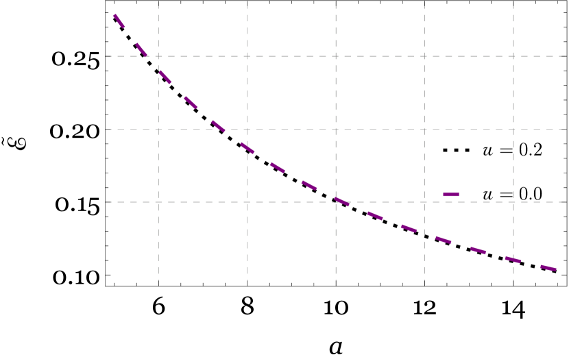
(a) Behaviour of ergotropy in NR limit.

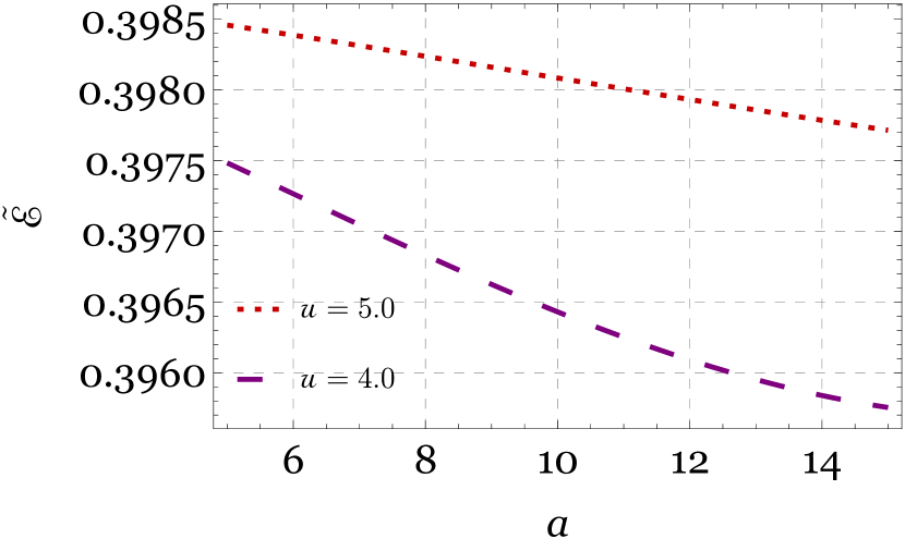
(b) Behaviour of ergotropy in UR limit.

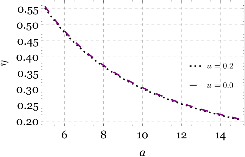
(c) Behaviour of charging efficiency in NR limit.

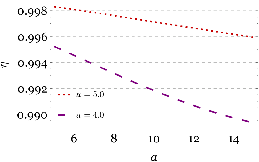
(d) Behaviour of charging efficiency in UR limit.

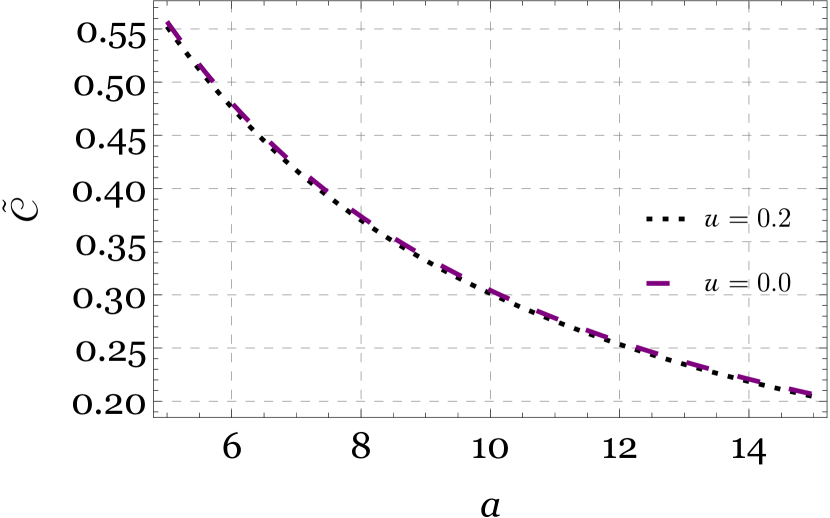
(e) Behaviour of capacity in NR limit.

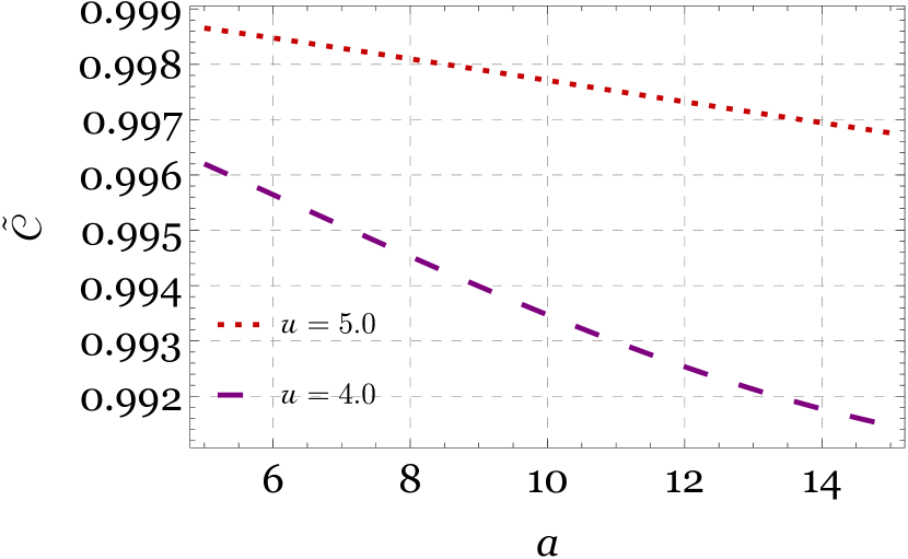
(f) Behaviour of capacity in UR limit.

Figure 1: Behaviour of different battery parameters with respect to $a$ in quadratic coupling scenario.

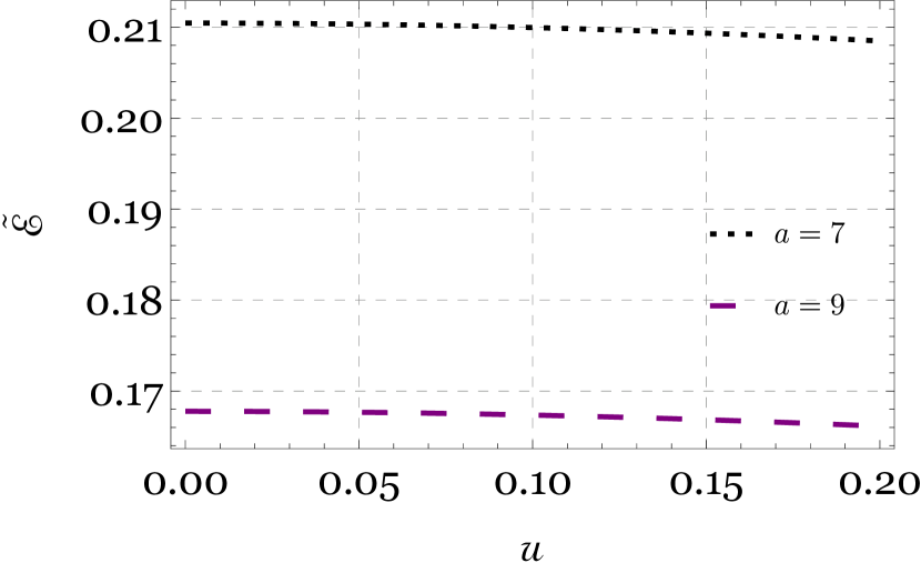
(a) Behaviour of ergotropy in NR limit.

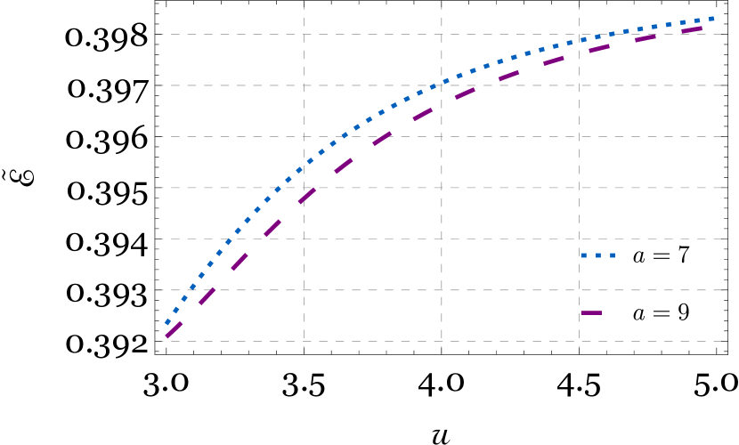
(b) Behaviour of ergotropy in UR limit.

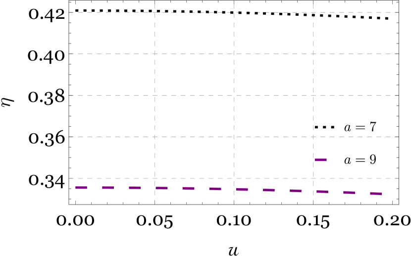
(c) Behaviour of charging efficiency in NR limit.

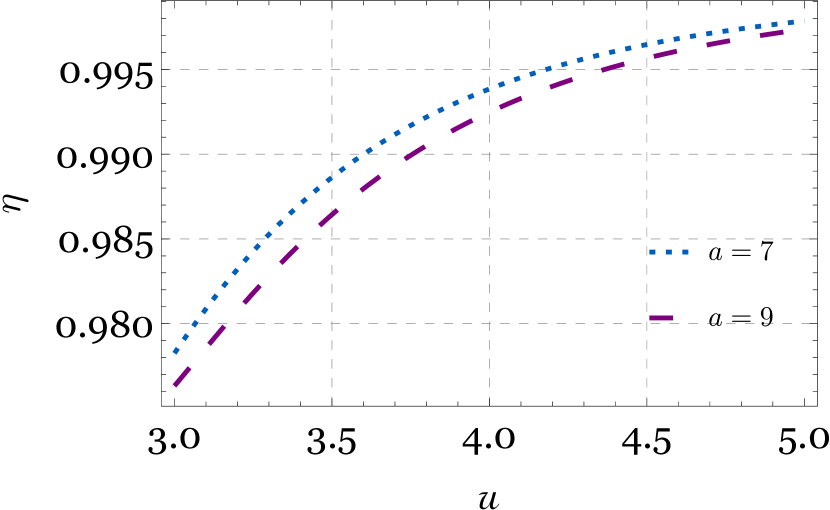
(d) Behaviour of charging efficiency in UR limit.

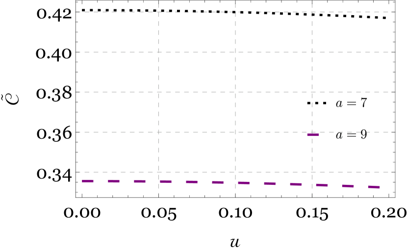
(e) Behaviour of capacity in NR limit.

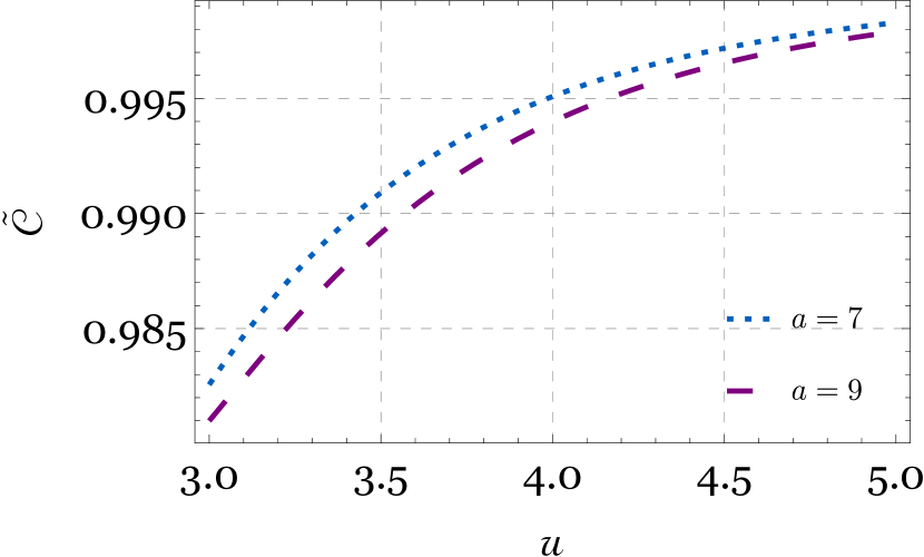
(f) Behaviour of capacity in UR limit.

Figure 2: Behaviour of different battery parameters with respect to $\mathcal{u}$.

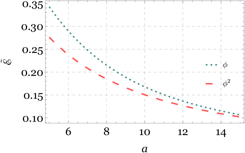
(a) Behaviour of ergotropy in NR limit, $\mathcal{u}=0.2$.

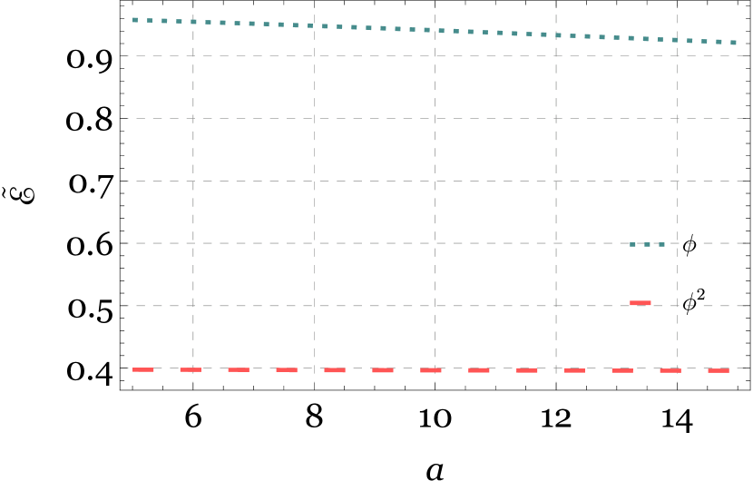
(b) Behaviour of ergotropy in UR limit, $\mathcal{u}=4$.

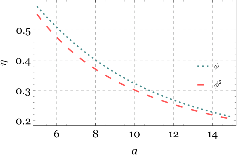
(c) Behaviour of charging efficiency in NR limit, $\mathcal{u}=0.2$.

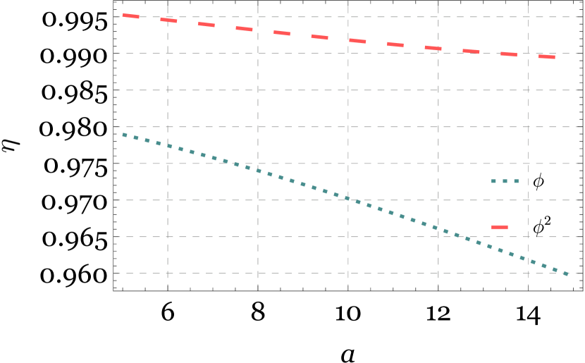
(d) Behaviour of charging efficiency in UR limit, $\mathcal{u}=4$.

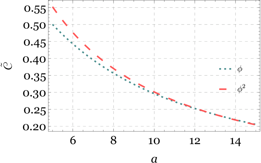
(e) Behaviour of capacity in NR limit, $\mathcal{u}=0.2$.

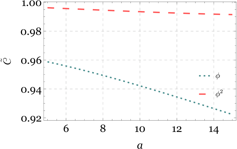
(f) Behaviour of capacity in UR limit, $\mathcal{u}=4$.

Figure 3: Behaviour of different battery parameters with respect to $a$ for the two coupling scenarios.

For both the limiting case, we choose two different $\mathcal{u}$ values. For the entire analysis values of $\mathcal{u}$ can be fixed using the relation $\mathcal{u}=\frac{\mathit{v}}{\sqrt{1-\mathit{v}^{2}}}$, where $\mathit{v}$ is the magnitude of the battery velocity. In the following Figures, we consider all the battery parameters and velocity $\mathcal{u}$ as dimensionless parameters. Other than this, we consider the dimensionless parameters $\tilde{a}$, $\tilde{\tau}$ as $a$, and $\tau$ respectively.

In Figs. (1(a), 1(b)), variation of the scaled ergotropy has been plotted for the NR and the UR limit, respectively.

From Fig. 1(a), we observe that when the velocity of the battery $\mathit{v}=0\,(\mathcal{u}=0)$, the ergotropy gradually decreases when we increase the acceleration. The decreasing trend in ergotropy is associated with decoherence resulting from the interaction between the battery and the massless scalar field. Taking into account, the effect of the velocity on the performance of the battery, we observe that for a fixed value of acceleration, increase in the velocity of the battery is unable to impact the value of ergotropy. Therefore, in the non-relativistic case, velocity of the battery can not suppress the decreasing trend in ergotropy. From Fig. 1(b), we observe a decreasing trend in ergotropy as the acceleration increases. In this scenario, we choose the battery velocities $\mathit{v}=0.97\,(\mathcal{u}=4)$ and $\mathit{v}=0.99\,(\mathcal{u}=5)$, respectively. We find that at very high velocities, the rate of change of ergotropy with respect to acceleration is much slower compared to the non-relativistic case. Furthermore, for a fixed acceleration, increasing the battery’s velocity from $\mathit{v}=0.97$ to $0.99\,(\mathcal{u}=4\rightarrow 5)$ leads to a significant increase in ergotropy. Therefore, in the UR limit, incorporating velocity effects enhances the performance of the quantum battery.

In Figs. (1(c), 1(d)) 1(f)) variation of the charging efficiency of the quantum battery is plotted for the NR and the UR limit, respectively. Similarly, in Figs. Fig. (1(e), 1(f)) variation of the capacity of the quantum battery is plotted for the NR and the UR limit, respectively. From the behaviour of the charging efficiency and the capacity, we observe a similar pattern of fall-off with respect to acceleration for both NR and UR limits. For a fixed value of acceleration, the value of both the charging efficiency and the capacity remains unaffected in the NR limit same even if we increases the value of the velocity. However, in the UR limit, we observe that decoherence effect on both the battery parameters is suppressed due to the effect of the four velocity. Moreover, for a fixed value of acceleration, here the increase of velocity leads to a significant enhancement in the battery efficiency and capacity.

VI.0.2 Behaviour of the quantum battery parameters with respect to velocity

In Fig. 2, the effect of the velocity on various quantum battery parameters is illustrated for both the NR and UR limits. For both the limiting case, we choose two different $a$ values.

In Fig. (2(a), 2(b)), variation of the scaled ergotropy is plotted for the NR and the UR limit, respectively. From Fig. 2(a), we observe that in the NR limit the ergotropy remains unaffected when we increase the value of $\mathcal{u}$, which is consistent with the result of Fig. 1(a). Next, in the UR limit we observe that for a fixed value of velocity, the value of ergotropy decreases when we increase the acceleration of the battery $a=7$ to $9$. From the Unruh effect, increase in acceleration leads to the system effectively interacting with a hotter thermal bath. Therefore, the thermal fluctuations act as a noisy environment, introducing randomness into the system’s quantum state and causing it to lose coherence. From Fig. 2(b), we observe that ergotropy significantly increases when we increase the velocity of the battery. In this scenario, we also observe that for a fixed value of velocity, the value of ergotropy decreases if we increase the acceleration of the battery.

In Figs. (2(c), 2(d)) variation of the charging efficiency of the quantum battery has been shown for the NR and the UR limit, respectively. Similarly, in Figs. (2(e), 2(f)) variation of the capacity of the quantum battery has been shown for the NR and the UR limit, respectively. From the behaviour of the charging efficiency and the capacity with respect to velocity for both NR and UR limits, we observe a similar trend with the ergotropy. There is hardly any impact in the NR limit. However, all the battery parameters rise significantly with increase of velocity in the UR limit. From the behaviour of all the quantum battery parameters, it is clearly observed that taking into account the velocity in a planeorthogonal to the acceleration leads to suppression of the decoherence effect on the system and hence, the overall performance of the quantum battery enhances significantly.

VI.0.3 Comparison between the linear and quadratic couplings

In order to compare the effect of the linear and the quadratic environmental coupling on the quantum battery, we study the three quantum battery parameters in both the NR and the UR regimes. In Fig. 3, the effect of the coupling on the different quantum battery parameters is plotted with respect to the acceleration $a$ in both the NR and UR regimes.

In Fig. 3(a), we study the behaviour of the scaled ergotropy in the NR regime. We observe that for a fixed value of the quantum battery velocity in the NR regime, for both linear and quadratic coupling the ergotropy gradually decreases when we increase the acceleration. The curves for the linear and quadratic cases are seen to approach each other for higher values of acceleration, showing that the nature of the field coupling doesn’t impact the dynamics significantly in the NR limit.

For the UR case, from Fig. 3(b), we observe that for a fixed value of the quantum battery velocity, the ergotrop decreases very slowly with acceleration for the linear coupling scenario. However, in case of quadratic coupling, we find that the ergotropy remains nearly unchanged. The latter behaviour indicates that in case of quadratic coupling if the battery velocity is high enough ($\mathit{v}\sim 0.97$), then there is no decoherence effect, and the quantum battery effectively behaves as a closed system. Such behaviour can also be observed if we place the quantum battery coupled with an environment in a cavity set-up [63]. Preservation of quantum coherence is crucial for the efficient operation of quantum devices like batteries.

In Figs. (3(c), 3(d)), we study the behaviour of the charging efficiency in the NR and UR regime, respectively. From Fig. 3(c) we observe that for a fixed value of the quantum battery velocity in the NR regime, for both linear and quadratic coupling the charging efficiency shows a similar trend like ergotropy. Charging efficiency gradually decreases when we increase the acceleration. For larger values of the acceleration, the dependency on the nature of the coupling reduces. In the UR regime, from Fig. 3(d), we observe that for a fixed value of the quantum battery velocity in the linear coupling scenario, the charging efficiency drops with the the acceleration. However, for quadratic coupling, we find that the charging efficiency reduces comparatively slowly. For a fixed value of $a$ and $\mathcal{u}$, we observe that the value of the charging efficiency is higher for the quadratic coupling than for the linear coupling. Therefore, this behaviour indicates that the quantitative enhancement of the performance of the quantum battery through quadratic coupling improves further with acceleration.

In Figs. (3(e), 3(f)), we study the behaviour of the battery capacity in the NR and UR regime, respectively. From Fig. 3(e), we again observe that in the NR regime, the nature of the environmental coupling is unable to impact much the battery performance. However, in the UR limit from Fig. 3(f), we observe that the battery capacity for the quadratic coupling turns out to be considerably higher compared to the case of linear coupling. This difference again grows with increase of acceleration, signifying that the performance of the quantum battery can be considerably enhanced through quadratic scalar field coupling.

VII Conclusions

In this study we investigate the relativistic effects on the performance of a quantum battery given in terms of the battery parameters, ergotropy, charging efficiency, and capacity. The quantum battery comprises a Unruh-De Witt detector which is charged through a coherent classical pulse [45, 46, 47]. At the time of charging, the battery interacts with the environment of a massless quantum scalar field. The trajectory of the battery is composed of uniform acceleration along one direction, combined with constant four-velocity components in the orthogonal plane to the acceleration. To explore the effect of the environment of the quantum battery, here we consider a nonlinear quadratic coupling between the quantum battery and the massless quantum scalar field [4, 52, 53, 54], and compare the results obtained with the linear coupling scenario.

A generic feature of quantum dynamics is the degradation of quantum resources such as coherence and entanglement in the relativistic arena [29, 30, 31, 32, 33, 34, 35, 36, 37, 38, 39]. The Uhruh effect implies an effective heat bath for accelerated systems resulting in deceoherence of quantum states. This trend is clearly observed through our computation of the battery parameters, all of which are seen to fall with acceleration. However, the presence of velocity components orthogonal to the direction of the acceleration enable reduction in the rate of loss of coherence, as again evident through our evaluation of the battery ergodicity, capacity and charging efficiency. Such a feature is absent in the non-relativistic limit where it is shown that battery velocity is unable to ward off the decohering effects of acceleration.

The role of the quadratic scalar field coupling becomes remarkably evident in the ultrarelativistic limit, leading to significant improvement in battery performance over that obtained through a linear environmental coupling. Though in absolute terms, the magnitude of the battery ergodicity for linear coupling exceeds that in the case of quadratic coupling, this effect seems to be more than compensated by the behaviour of antiergodicity. The quantum battery capacity, taking into account both the ergodicity and antiergodicity, encodes the overall figure of merit for storing energy [44]. Our results show that battery capacity is much better preserved through quadratic coupling under acceleration.

Similarly, we find that the difference in the charging efficiency between the quadratic and linear coupling scenarios grows with acceleration, again providing a striking example of enhancement of the quantum battery performance through quadratic environmental coupling in the relativistic scenario. The analysis contained in the present work inspires related investigations into the behavior of other quantities of interest in quantum thermodynamics [64] in the presense of nonlinear environmental couplings. Moreover, in the upcoming scenario for development of quantum technologies, formulation of techniques to preserve quantum coherence through environmental engineering is likely to play a key role [55, 56]. Our results should motivate further studies on different types of environmental couplings for quantum heat engines in relativistic regimes.

References

- [1] R. Kosloff, “Quantum thermodynamics: A dynamical viewpoint”, Entropy 15[6] (2013) 2100, URL.
- [2] S. Vinjanampathy and J. Anders, “Quantum thermodynamics”, Contemporary Physics 57[4] (2016) 545–579.
- [3] S. Bhattacharjee and A. Dutta, “Quantum thermal machines and batteries”, The European Physical Journal B 94[12] (2021) 239.
- [4] R. Alicki and M. Fannes, “Entanglement boost for extractable work from ensembles of quantum batteries”, Phys. Rev. E 87 (2013) 042123.
- [5] F. Campaioli, F. A. Pollock and S. Vinjanampathy, “Quantum Batteries”, in Thermodynamics in the Quantum Regime: Fundamental Aspects and New Directions (edited by F. Binder, L. A. Correa, C. Gogolin, J. Anders and G. Adesso), p. 207–225, Springer International Publishing, Cham 2018.
- [6] M. Campisi, P. Hänggi and P. Talkner, “Colloquium: Quantum fluctuation relations: Foundations and applications”, Rev. Mod. Phys. 83 (2011) 771.
- [7] M. Horodecki and J. Oppenheim, “Fundamental limitations for quantum and nanoscale thermodynamics”, Nature Communications 4[1] (2013) 2059.
- [8] J. Goold, M. Huber, A. Riera, L. del Rio and P. Skrzypczyk, “The role of quantum information in thermodynamics—a topical review”, Journal of Physics A: Mathematical and Theoretical 49[14] (2016) 143001.
- [9] F. C. Binder, S. Vinjanampathy, K. Modi and J. Goold, “Quantacell: powerful charging of quantum batteries”, New Journal of Physics 17[7] (2015) 075015.
- [10] F. Campaioli, F. A. Pollock, F. C. Binder, L. Céleri, J. Goold, S. Vinjanampathy and K. Modi, “Enhancing the Charging Power of Quantum Batteries”, Phys. Rev. Lett. 118 (2017) 150601.
- [11] D. Farina, G. M. Andolina, A. Mari, M. Polini and V. Giovannetti, “Charger-mediated energy transfer for quantum batteries: An open-system approach”, Phys. Rev. B 99 (2019) 035421.
- [12] Y.-Y. Zhang, T.-R. Yang, L. Fu and X. Wang, “Powerful harmonic charging in a quantum battery”, Phys. Rev. E 99 (2019) 052106.
- [13] J. Carrasco, J. R. Maze, C. Hermann-Avigliano and F. Barra, “Collective enhancement in dissipative quantum batteries”, Phys. Rev. E 105 (2022) 064119.
- [14] R. R. Rodríguez, B. Ahmadi, P. Mazurek, S. Barzanjeh, R. Alicki and P. Horodecki, “Catalysis in charging quantum batteries”, Phys. Rev. A 107 (2023) 042419.
- [15] G. Gemme, G. M. Andolina, F. M. D. Pellegrino, M. Sassetti and D. Ferraro, “Off-Resonant Dicke Quantum Battery: Charging by Virtual Photons”, Batteries 9[4], URL.
- [16] G. Gemme, M. Grossi, S. Vallecorsa, M. Sassetti and D. Ferraro, “Qutrit quantum battery: Comparing different charging protocols”, Phys. Rev. Res. 6 (2024) 023091.
- [17] W.-L. Song, H.-B. Liu, B. Zhou, W.-L. Yang and J.-H. An, “Remote Charging and Degradation Suppression for the Quantum Battery”, Phys. Rev. Lett. 132 (2024) 090401.
- [18] J. Q. Quach, K. E. McGhee, L. Ganzer, D. M. Rouse, B. W. Lovett, E. M. Gauger, J. Keeling, G. Cerullo, D. G. Lidzey and T. Virgili, “Superabsorption in an organic microcavity: Toward a quantum battery”, Science Advances 8[2] (2022) eabk3160.
- [19] G. Gemme, M. Grossi, D. Ferraro, S. Vallecorsa and M. Sassetti, “IBM Quantum Platforms: A Quantum Battery Perspective”, Batteries 8[5], URL.
- [20] C.-K. Hu, J. Qiu, P. J. P. Souza, J. Yuan, Y. Zhou, L. Zhang, J. Chu, X. Pan, L. Hu, J. Li, Y. Xu, Y. Zhong, S. Liu, F. Yan, D. Tan, R. Bachelard, C. J. Villas-Boas, A. C. Santos and D. Yu, “Optimal charging of a superconducting quantum battery”, Quantum Science and Technology 7[4] (2022) 045018.
- [21] I. Maillette de Buy Wenniger, S. E. Thomas, M. Maffei, S. C. Wein, M. Pont, N. Belabas, S. Prasad, A. Harouri, A. Lemaître, I. Sagnes, N. Somaschi, A. Auffèves and P. Senellart, “Experimental Analysis of Energy Transfers between a Quantum Emitter and Light Fields”, Phys. Rev. Lett. 131 (2023) 260401.
- [22] M. Carrega, A. Crescente, D. Ferraro and M. Sassetti, “Dissipative dynamics of an open quantum battery”, New Journal of Physics 22[8] (2020) 083085.
- [23] F. T. Tabesh, F. H. Kamin and S. Salimi, “Environment-mediated charging process of quantum batteries”, Phys. Rev. A 102 (2020) 052223.
- [24] C.-Y. Lu, Y. Cao, C.-Z. Peng and J.-W. Pan, “Micius quantum experiments in space”, Rev. Mod. Phys. 94 (2022) 035001.
- [25] D. Ribezzo, M. Zahidy, I. Vagniluca, N. Biagi, S. Francesconi, T. Occhipinti, L. K. Oxenløwe, M. Lončarić, I. Cvitić, M. Stipčević, Ž. Pušavec, R. Kaltenbaek, A. Ramšak, F. Cesa, G. Giorgetti, F. Scazza, A. Bassi, P. De Natale, F. S. Cataliotti, M. Inguscio, D. Bacco and A. Zavatta, “Deploying an Inter-European Quantum Network”, Advanced Quantum Technologies 6[2] (2023) 2200061.
- [26] S. A. Fulling, “Nonuniqueness of Canonical Field Quantization in Riemannian Space-Time”, Phys. Rev. D 7 (1973) 2850.
- [27] P. C. W. Davies, “Scalar production in Schwarzschild and Rindler metrics”, Journal of Physics A: Mathematical and General 8[4] (1975) 609.
- [28] W. G. Unruh, “Notes on black-hole evaporation”, Phys. Rev. D 14 (1976) 870.
- [29] M. Ahmadi, D. E. Bruschi and I. Fuentes, “Quantum metrology for relativistic quantum fields”, Phys. Rev. D 89 (2014) 065028.
- [30] A. G. S. Landulfo and G. E. A. Matsas, “Sudden death of entanglement and teleportation fidelity loss via the Unruh effect”, Phys. Rev. A 80 (2009) 032315.
- [31] Y. Huang, K. Yan, Y. Wu and X. Hao, “Decoherence of quantum parameter estimation for open Dirac particle in Garfinkle–Horowitz–Strominger dilation black hole”, The European Physical Journal C 79[11] (2019) 974.
- [32] Z. Zhao, Q. Pan and J. Jing, “Quantum estimation of acceleration and temperature in open quantum system”, Phys. Rev. D 101 (2020) 056014.
- [33] H. Du and R. B. Mann, “Fisher information as a probe of spacetime structure: relativistic quantum metrology in (A)dS”, Journal of High Energy Physics 2021[5] (2021) 112.
- [34] X. Liu, J. Jing, Z. Tian and W. Yao, “Does relativistic motion always degrade quantum Fisher information?”, Phys. Rev. D 103 (2021) 125025.
- [35] F. Benatti and R. Floreanini, “Entanglement generation in uniformly accelerating atoms: Reexamination of the Unruh effect”, Phys. Rev. A 70 (2004) 012112.
- [36] B. L. Hu, S.-Y. Lin and J. Louko, “Relativistic quantum information in detectors–field interactions”, Classical and Quantum Gravity 29[22] (2012) 224005.
- [37] D. Moustos and C. Anastopoulos, “Non-Markovian time evolution of an accelerated qubit”, Phys. Rev. D 95 (2017) 025020.
- [38] R. Chatterjee and A. S. Majumdar, “Preservation of quantum coherence under Lorentz boost for narrow uncertainty wave packets”, Phys. Rev. A 96 (2017) 052301.
- [39] B. Sokolov, J. Louko, S. Maniscalco and I. Vilja, “Unruh effect and information flow”, Phys. Rev. D 101 (2020) 024047.
- [40] E. Arias, T. R. de Oliveira and M. Sarandy, “The unruh quantum otto engine”, Journal of High Energy Physics 2018[2].
- [41] A. Mukherjee, S. Gangopadhyay and A. S. Majumdar, “Unruh quantum Otto engine in the presence of a reflecting boundary”, Journal of High Energy Physics 2022[9] (2022) 105.
- [42] A. E. Allahverdyan, R. Balian and T. M. Nieuwenhuizen, “Maximal work extraction from finite quantum systems”, Europhysics Letters 67[4] (2004) 565.
- [43] S. Julià-Farré, T. Salamon, A. Riera, M. N. Bera and M. Lewenstein, “Bounds on the capacity and power of quantum batteries”, Phys. Rev. Res. 2 (2020) 023113.
- [44] X. Yang, Y.-H. Yang, M. Alimuddin, R. Salvia, S.-M. Fei, L.-M. Zhao, S. Nimmrichter and M.-X. Luo, “Battery Capacity of Energy-Storing Quantum Systems”, Phys. Rev. Lett. 131 (2023) 030402.
- [45] B. Mojaveri, R. Jafarzadeh Bahrbeig, M. A. Fasihi and S. Babanzadeh, “Enhancing the direct charging performance of an open quantum battery by adjusting its velocity”, Scientific Reports 13[1] (2023) 19827.
- [46] X. Hao, K. Yan, J. Tan and Q.-Y. Wu, “Quantum work extraction of an accelerated Unruh-DeWitt battery in relativistic motion”, Phys. Rev. A 107 (2023) 012207.
- [47] S. Abdolrahimi, “Velocity effects on an accelerated Unruh–DeWitt detector”, Classical and Quantum Gravity 31[13] (2014) 135009.
- [48] B. DeWitt, General Relativity: An Einstein Centenary Survey, Cambridge University Press, Cambridge, U.K. 1979.
- [49] W. G. Unruh and R. M. Wald, “What happens when an accelerating observer detects a Rindler particle”, Phys. Rev. D 29 (1984) 1047.
- [50] A. Pozas-Kerstjens and E. Martín-Martínez, “Entanglement harvesting from the electromagnetic vacuum with hydrogenlike atoms”, Phys. Rev. D 94 (2016) 064074.
- [51] D. Wu, S.-C. Tang and Y. Shi, “Birth and death of entanglement between two accelerating Unruh-DeWitt detectors coupled with a scalar field”, Journal of High Energy Physics 2023[12] (2023) 37.
- [52] D. Hümmer, E. Martín-Martínez and A. Kempf, “Renormalized Unruh-DeWitt particle detector models for boson and fermion fields”, Phys. Rev. D 93 (2016) 024019.
- [53] A. Sachs, R. B. Mann and E. Martín-Martínez, “Entanglement harvesting and divergences in quadratic Unruh-DeWitt detector pairs”, Phys. Rev. D 96 (2017) 085012.
- [54] F. Gray and R. B. Mann, “Scalar and fermionic Unruh Otto engines”, Journal of High Energy Physics 2018[11] (2018) 174.
- [55] C. P. Koch, “Controlling open quantum systems: tools, achievements, and limitations”, Journal of Physics: Condensed Matter 28[21] (2016) 213001.
- [56] C. Uchiyama, W. J. Munro and K. Nemoto, “Environmental engineering for quantum energy transport”, npj Quantum Information 4[1] (2018) 33.
- [57] M. O. Scully and M. S. Zubairy, Quantum optics, Cambridge university press 1997, URL.
- [58] N. D. Birrell and P. Davies, Quantum fields in curved space, Cambridge university press 1984, URL.
- [59] R. Chatterjee, S. Gangopadhyay and A. S. Majumdar, “Violation of equivalence in an accelerating atom-mirror system in the generalized uncertainty principle framework”, Phys. Rev. D 104 (2021) 124001.
- [60] A. Mukherjee, S. Gangopadhyay and A. S. Majumdar, “Fulling-Davies-Unruh effect for accelerated two-level single and entangled atomic systems”, Phys. Rev. D 108 (2023) 085018.
- [61] V. Gorini, A. Kossakowski and E. C. G. Sudarshan, “Completely positive dynamical semigroups of N‐level systems”, Journal of Mathematical Physics 17[5] (1976) 821.
- [62] G. Lindblad, “On the generators of quantum dynamical semigroups”, Communications in Mathematical Physics 48[2] (1976) 119.
- [63] Y. Jin and H. Yu, “Electromagnetic shielding in quantum metrology”, Phys. Rev. A 91 (2015) 022120.
- [64] N. M. Myers, O. Abah and S. Deffner, “Quantum thermodynamic devices: From theoretical proposals to experimental reality”, AVS Quantum Science 4[2] (2022) 027101.