Study of $B\rightarrow\rho\eta$, $\rho\eta^{\prime}$ decays in the modified perturbative QCD approach

Abstract

We study the decay processes of $B\rightarrow\rho\eta$, $\rho\eta^{\prime}$ in perturbative QCD approach with a few improvements incorproated in it, where the contributions with large momentum transfer are calculated perturbatively, and the contributions with lower energy scale are treated by introuducing soft transition form factors. In addition, color-octet conributions are introduced which are essentially long-distance contributions. With resonanble input parameters selected, we find that the theoretical results of the branching ratios and $CP$ violations are all consistent with experimental data. We also predict some unmeasured quantities, which can be tested by experiment in the future.

I Introduction

$B$ decays are important for testing the standard model about the properties of weak interaction. It is not only weak interaction but also strong interactiosn are involved in $B$ decays. So it is very challenging for developing theoretical method to deal with strong interactions in $B$ decays. Several methods of treating QCD effects have been developed in theory several decades before, such as perturbative QCD (PQCD) approach based on $k_{t}$ factorization PQCD1 ; PQCD2 ; PQCD3 and QCD factorization (QCDF) approach base on collinear factorization QCDf1 ; QCDf2 ; QCDf3 ; QCDf4 etc. As more and more precise data having been collected by $B$ factories PDG2024 , several deviations between theoretical predictions for branching ratios and $CP$ violations of nonleptonic decays and experimantal data have been found, which are called $B\to K\pi$ and $B\to\pi\pi$ puzzles BFRS2003 ; LMS2005 ; LM2011 ; LM2014 . Including QCD effeccts of next-to-leading order can partially solve these problems and partially not in PQCD LMS2005 ; ZLFCX2014 ; Baietall2014 and QCDF BY2006 ; BJ2006 ; Bell2008 ; Pilipp2008 ; BHL2010 . There are also deviations between theory and experimental data in other nonleptonic two-body decay modes of $B$ meson C2022 . New ingredients or nonperturbative inputs are needed to diminish these deviations CC2009a ; CC2009b ; CCSYL2014 ; LLJ2016 .

Previously new mecnanisms were developed based on the PQCD approach LY2021 ; LY2023 ; WY2023 ; LWY2024 , where $B$ meson wave function from relativistic potential model is used, the infrared cutoff scale $\mu_{c}$, the soft transition form factros and color-octet contributions are introduced. The contributions with the scale higher than the cutoff scale $\mu_{c}$ are calculated with PQCD approach, while the contributions with the scale lower than $\mu_{c}$ are considered in terms of the soft form factors. The calculations based on the modified PQCD approacn can well explain the experimental data of all the $B\to PP$ decay modes LWY2024 , where $P$ stands for pseudoscale meons.

In this work we study the $B\rightarrow\rho\eta$, $\rho\eta^{\prime}$ decays in this modified perturbative QCD approach. The branching ratios and $CP$ violations are calculated. With resonable input parameters taken, the theoretical result can be well consistent with experimental measurement. We also predict some unmeasured branching ratios and $CP$ violations, which can be tested in experiment in the future.

The remaining part of this paper is organized as follows. The hard contributions of leading oder in QCD are given in Sec. II. The perturbation contributions of next-to-leading oder in QCD are presented in Sec. III. The contribution of soft transition form factors can be found in sec. IV. Section V is for contributions of color-octet quark-antiquark pairs that finally form the final state mesons. Section VI is the numerical result and discusions. Finally section VII is a brief summary.

II The hard amplitude of leading-order in perturbative QCD

II.1 The Effective Hamiltonian

The effective Hamiltonian of charmless hadronic weak decay of $B$ meson caused by the $b\rightarrow d$ transition is Hamiltanion1996

$$\mathcal{H}_{\mathrm{eff}} = \frac{G_{F}}{\sqrt{2}}[V_{u}(C_{1}O_{1}^{u}+C_{2}O_{2}^{u})$$ (1)

$$-V_{t}\sum_{i=3}^{10}C_{i}O_{i}-V_{t}C_{8g}O_{8g}],$$

where $V_{u}=V_{ub}V_{ud}^{*}$ and $V_{t}=V_{tb}V_{td}^{*}$ are products of Cabibbo-Kobayashi-Maskawa (CKM) matrix elements, $G_{F}=1.16638\times 10^{-5}~{}\mathrm{GeV}^{-2}$ is the Fermi constant, and $C_{i}$’s are the Wilson coefficients. The operators in the effective Hamiltonian are given as

$$O_{1}^{u}=\bar{d}_{\alpha}\gamma^{\mu}(1-\gamma_{5})u_{\beta}\bar{u}_{\beta}\gamma_{\mu}(1-\gamma_{5})b_{\alpha},$$

$$O_{2}^{u}=\bar{d}_{\alpha}\gamma^{\mu}(1-\gamma_{5})u_{\alpha}\bar{u}_{\beta}\gamma_{\mu}(1-\gamma_{5})b_{\beta},$$

$$O_{3}=\bar{d}_{\alpha}\gamma^{\mu}(1-\gamma_{5})b_{\alpha}\sum_{q^{\prime}}\bar{q}^{\prime}_{\beta}\gamma_{\mu}(1-\gamma_{5})q^{\prime}_{\beta},$$

$$O_{4}=\bar{d}_{\alpha}\gamma^{\mu}(1-\gamma_{5})b_{\beta}\sum_{q^{\prime}}\bar{q}^{\prime}_{\beta}\gamma_{\mu}(1-\gamma_{5})q^{\prime}_{\alpha},$$

$$O_{5}=\bar{d}_{\alpha}\gamma^{\mu}(1-\gamma_{5})b_{\alpha}\sum_{q^{\prime}}\bar{q}^{\prime}_{\beta}\gamma_{\mu}(1+\gamma_{5})q^{\prime}_{\beta},$$

$$O_{6}=\bar{d}_{\alpha}\gamma^{\mu}(1-\gamma_{5})b_{\beta}\sum_{q^{\prime}}\bar{q}^{\prime}_{\beta}\gamma_{\mu}(1+\gamma_{5})q^{\prime}_{\alpha},$$

$$O_{7}=\frac{3}{2}\bar{d}_{\alpha}\gamma^{\mu}(1-\gamma_{5})b_{\alpha}\sum_{q^{\prime}}e_{q^{\prime}}\bar{q}^{\prime}_{\beta}\gamma_{\mu}(1+\gamma_{5})q^{\prime}_{\beta},$$

$$O_{8}=\frac{3}{2}\bar{d}_{\alpha}\gamma^{\mu}(1-\gamma_{5})b_{\beta}\sum_{q^{\prime}}e_{q^{\prime}}\bar{q}^{\prime}_{\beta}\gamma_{\mu}(1+\gamma_{5})q^{\prime}_{\alpha},$$

$$O_{9}=\frac{3}{2}\bar{d}_{\alpha}\gamma^{\mu}(1-\gamma_{5})b_{\alpha}\sum_{q^{\prime}}e_{q^{\prime}}\bar{q}^{\prime}_{\beta}\gamma_{\mu}(1-\gamma_{5})q^{\prime}_{\beta},$$

$$O_{10}=\frac{3}{2}\bar{d}_{\alpha}\gamma^{\mu}(1-\gamma_{5})b_{\beta}\sum_{q^{\prime}}e_{q^{\prime}}\bar{q}^{\prime}_{\beta}\gamma_{\mu}(1-\gamma_{5})q^{\prime}_{\alpha},$$

$$O_{8\textsl{g}}=\frac{g_{s}}{8\pi^{2}}m_{b}\bar{d}_{\alpha}\sigma^{\mu\nu}(1+\gamma_{5})T^{a}_{\alpha\beta}b_{\beta}G_{\mu\nu}^{a},$$ (2)

where $\alpha$ and $\beta$ are color indices. The summation of $q^{\prime}$ includes $u,d,s,c$ and $b$ quarks.

II.2 The Factorization of Decay Amplitude and The Meson Wave Functions

In $B$ decays, when the momentum of the gluons exchanged between quarks exceeds the critical cutoff scale $\mu_{c}$ which used to separate the soft and hard contributions, the decay amplitude can be factorized as the convolution of hard scattering amplitude and meson wave functions

$$\mathcal{M} = \int d^{3}k\int d^{3}k_{1}\int d^{3}k_{2}\Phi^{B}(\vec{k},\mu)C(\mu)$$ (3)

$$\times H(k,k_{1},k_{2},\mu)\Phi^{\eta_{q(s)}}(k_{1},\mu)\Phi^{\rho}(k_{2},\mu),$$

where $H$ is the hard scattering amplitude that can be calculated by using perturbative theory, $C(\mu)$ are the Wilson coefficients. $\Phi^{B},\Phi^{\eta_{q(s)}}$ and $\Phi^{\rho}$ are the meson wave functions which can be used to absorb non-perturbative soft interactions.

The $B$ meson spinor wave function can be defined by the matrix element $\langle 0|\bar{q}(z)_{\beta}[z,0]b(0)_{\alpha}|\bar{B}\rangle$ as

$$\langle 0|\bar{q}(z)_{\beta}[z,0]b(0)_{\alpha}|\bar{B}\rangle=\int d^{3}k\Phi^{B}_{\alpha\beta}(\vec{k})e^{-ik\cdot z},$$ (4)

where $[z,0]={\cal P}\exp[-ig_{s}T^{a}\int_{0}^{1}d\alpha z^{\mu}A_{\mu}^{a}(\alpha z)]$, which is the path-ordered exponential introduced to maintain the gauge invariance of the spinor wave function.

In the rest-frame of the $B$ meson, the wave function $\Phi^{B}_{\alpha\beta}(\vec{k})$ can be obtained by solving the bound-state equation within the QCD-inspired relativistic potential model Yang2012 ; LY2014 ; LY2015 ; SY2017 ; SY2019 , which is

$$\Phi_{\alpha\beta}^{B}(\vec{k}) = \frac{-if_{B}m_{B}}{4}K(\vec{k})$$ (5)

$$\cdot\Bigg{\{}(E_{Q}+m_{Q})\frac{1+\not{v}}{2}\Bigg{[}\Bigg{(}\frac{k^{+}}{\sqrt{2}}+\frac{m_{q}}{2}\Bigg{)}\not{n}_{+}$$

$$+\Bigg{(}\frac{k^{-}}{\sqrt{2}}+\frac{m_{q}}{2}\Bigg{)}\not{n}_{-}-k_{\perp}^{\mu}\gamma_{\mu}\Bigg{]}\gamma^{5}$$

$$-(E_{q}+m_{q})\frac{1-\not{v}}{2}\Bigg{[}\Bigg{(}\frac{k^{+}}{\sqrt{2}}-\frac{m_{q}}{2}\Bigg{)}\not{n}_{+}$$

$$+\Bigg{(}\frac{k^{-}}{\sqrt{2}}-\frac{m_{q}}{2}\Bigg{)}\not{n}_{-}-k_{\perp}^{\mu}\gamma_{\mu}\Bigg{]}\gamma^{5}\Bigg{\}}_{\alpha\beta},$$

where $f_{B}$ is the decay constant of $B$ meson, $m_{B}$ the meson mass, and $Q$ and $q$ represent the $b$ and light quarks in $B$ meson, respectively. $v$ is the four-speed which satisfies $v^{\mu}=(1,0,0,0)$. $n_{\pm}^{\mu}=(1,0,0,\mp 1)$ are two lightlike vectors. $k_{\pm}$ and $k_{\perp}$ are defined by

$$k_{\pm}=\dfrac{k^{0}\pm k^{3}}{\sqrt{2}},k_{\perp}^{\mu}=(0,k^{1},k^{2},0),$$ (6)

where $k$ is the momentum of the light quark in the rest-frame of $B$ meson.

$\Psi_{0}(\vec{k})$ represents the wave function of $B$ meson in its rest-frame

$$\Psi_{0}(\vec{k})=a_{1}e^{a_{2}|\vec{k}|^{2}+a_{3}|\vec{k}|+a_{4}},$$ (7)

where the parameters are SY2017

$$a_{1}=4.55_{-0.30}^{+0.40}\,\mathrm{GeV}^{-3/2},\quad\;a_{2}=-0.39_{-0.20}^{+0.15}\,\mathrm{GeV}^{-2},$$

$$a_{3}=-1.55\pm 0.20\,\mathrm{GeV}^{-1},\quad a_{4}=-1.10_{-0.05}^{+0.10}.$$ (8)

The function $K(\vec{k})$ represents a quantity involving the wave function of $B$ meson

$$K(\vec{k})=\frac{2N_{B}\Psi_{0}(\vec{k})}{\sqrt{E_{q}E_{Q}(E_{q}+m_{q})(E_{Q}+m_{Q})}},$$ (9)

where $N_{B}=\dfrac{1}{f_{B}}\sqrt{\dfrac{3}{(2\pi)^{3}m_{B}}}$ is the normalization constant.

The definition of the light-cone wave functions for the $\eta_{q}$ and $\eta_{s}$ mesons is similar to that of the $\pi$ meson bra1990 ; bal1999

$$\langle\eta_{q(s)}(p_{\eta_{q(s)}})|\bar{q}(y)_{\gamma}q^{\prime}(0)_{\delta}|0\rangle = \int dxd^{2}k_{q\perp}e^{i(xp_{\eta_{q(s)}}\cdot y-y_{\perp}\cdot k_{q\perp})}$$ (10)

$$\times\Phi^{\eta_{q(s)}}_{\delta\gamma}.$$

In the momentum space, the spinor wave function $\Phi^{\eta_{q(s)}}_{\delta\gamma}$ can be written as bf2001 ; wy2002

$$\Phi^{\eta_{q(s)}}_{\delta\gamma} = \frac{if_{q(s)}}{4}\Bigg{\{}\not{p}_{\eta_{q(s)}}\gamma_{5}\phi_{\eta_{q(s)}}(x,k_{q\perp})-\mu_{\eta_{q(s)}}\gamma_{5}$$ (11)

$$\times\Bigg{[}\phi^{\eta_{q(s)}}_{P}(x,k_{q\perp})$$

$$-i\sigma_{\mu\nu}\frac{p_{\eta_{q(s)}}^{\mu}\bar{p}_{\eta_{q(s)}}^{\nu}}{p_{\eta_{q(s)}}\cdot\bar{p}_{\eta_{q(s)}}}\frac{\phi^{\prime\eta_{q(s)}}_{\sigma}(x,k_{q\perp})}{6}$$

$$+i\sigma_{\mu\nu}p_{\eta_{q(s)}}^{\mu}\frac{\phi^{\eta_{q(s)}}_{\sigma}(x,k_{q\perp})}{6}\frac{\partial}{\partial k_{q\perp\nu}}\Bigg{]}\Bigg{\}}_{\delta\gamma},$$

where $f_{q(s)}$ is the decay constant for the $\eta_{q(s)}$ meson. $\mu_{\eta_{q(s)}}$ is the chiral mass. $\phi_{\eta_{q(s)}}$, $\phi^{\eta_{q(s)}}_{P}$ and $\phi^{\eta_{q(s)}}_{\sigma}$ are twist-2 and twist-3 distribution amplitudes, respectively. $\bar{p}_{\eta_{q(s)}}=(E_{\eta_{q(s)}},-\vec{p}_{\eta_{q(s)}})$ with $E_{\eta_{q(s)}}$ and $\vec{p}_{\eta_{q(s)}}$ are the energy and momentum of $\eta_{q(s)}$ meson. In addition, $\phi^{\prime\eta_{q(s)}}_{\sigma}(x,k_{q\perp})=\partial\phi^{\eta_{q(s)}}_{\sigma}(x,k_{q\perp})/\partial x$.

In $B\rightarrow\rho\eta^{(\prime)}$ decays, the $\rho$ meson is longitudinally polarized and its wave function in longitudinal polarization can be defined as TK-HNL ; Ball-Braun1998

$$\langle\rho(p_{\rho},\epsilon_{L})|\bar{q}(y)_{\gamma}q^{\prime}(0)_{\delta}|0\rangle = \int dxd^{2}k_{q\perp}e^{i(xp_{\rho}\cdot y-y_{\perp}\cdot k_{q\perp})}$$ (12)

$$\times\Phi^{\rho}_{\delta\gamma},$$

where

$$\varPhi_{\delta\gamma}^{\rho} = \dfrac{f_{\rho}^{||}}{4}[\epsilon\!\!\!/_{L}m_{\rho}\phi_{\rho}(x,k_{q\perp})+r_{f}\epsilon\!\!\!/_{L}p\!\!\!/_{\rho}\phi_{\rho}^{t}(x,k_{q\perp})$$ (13)

$$+r_{f}m_{\rho}\phi_{\rho}^{s}(x,k_{q\perp})]_{\delta\gamma},$$

with $r_{f}=f_{\rho}^{\perp}/f_{\rho}^{||}$. $f_{\rho}^{||}$ and $f_{\rho}^{\perp}$ are the longitudinal and transverse decay constants for $\rho$ meson, and $m_{\rho}$ is the meson mass. $\epsilon_{L}$ is the longitudinal polarization vector for $\rho$ meson. $\phi_{\rho}$, $\phi_{\rho}^{t}$ and $\phi_{\rho}^{s}$ are twist-2 and twist-3 distribution amplitudes, respectively.

II.3 The Mixing Scheme of $\eta-\eta^{\prime}$

We consider the mixing scheme of $\eta$ and $\eta^{\prime}$ mesons suggested by Feldmann, Kroll and Stech FKS1 ; FKS2 . The physical states $\ket{\eta}$ and $\ket{\eta^{\prime}}$ are expressed as a linear combination of orthogonal quark-flavor basis

$$\left(\begin{array}[]{c}\eta\\ \eta^{\prime}\end{array}\right)=\left(\begin{array}[]{cc}\cos\phi&-\sin\phi\\ \sin\phi&\cos\phi\end{array}\right)\left(\begin{array}[]{l}\eta_{q}\\ \eta_{s}\end{array}\right),$$ (14)

where $\eta_{q}=(u\bar{u}+d\bar{d})/\sqrt{2}$, $\eta_{s}=s\bar{s}$, and $\phi$ is the mixing angle. The decay constants for $\eta_{q}$ and $\eta_{s}$ are defined as follows

$$\langle 0|j^{q\mu}_{5}|\eta_{q}(p)\rangle=if_{q}p^{\mu},~{}~{}~{}\langle 0|j^{s\mu}_{5}|\eta_{s}(p)\rangle=if_{s}p^{\mu},$$ (15)

where $j^{q\mu}_{5}=\frac{\bar{u}\gamma^{\mu}\gamma_{5}u+\bar{d}\gamma^{\mu}\gamma_{5}d}{\sqrt{2}}$, $j^{s\mu}_{5}=\bar{s}\gamma^{\mu}\gamma_{5}s$, and

$$\begin{array}[]{ll}\langle 0|\bar{q}\gamma^{\mu}\gamma_{5}q|\eta(p)\rangle=if_{\eta}^{q}p^{\mu},&\langle 0|j^{s\mu}_{5}|\eta(p)\rangle=if_{\eta}^{s}p^{\mu},\\ \langle 0|\bar{q}\gamma^{\mu}\gamma_{5}q|\eta^{\prime}(p)\rangle=if_{\eta^{\prime}}^{q}p^{\mu},&\langle 0|j^{s\mu}_{5}|\eta^{\prime}(p)\rangle=if_{\eta^{\prime}}^{s}p^{\mu},\end{array}$$ (16)

here $q=u,d$. The relations between the decay constants are

$$\begin{array}[]{ll}f_{\eta}^{q}=\frac{f_{q}}{\sqrt{2}}\cos\phi,&f_{\eta}^{s}=-f_{s}\sin\phi,\\ &\\ f_{\eta^{\prime}}^{q}=\frac{f_{q}}{\sqrt{2}}\sin\phi,&f_{\eta^{\prime}}^{s}=f_{s}\cos\phi.\end{array}$$ (17)

The values of the decay constants and the mixing angle are taken as FKS1 ; FKS2

$$\begin{gathered}f_{q}=(1.07\pm 0.02)f_{\pi},\quad f_{s}=(1.34\pm 0.06)f_{\pi},\\ \phi=39.3^{\circ}\pm 1.0^{\circ},\end{gathered}$$ (18)

where $f_{\pi}=0.130\;\mathrm{GeV}$. The chiral masses for $\eta_{q}$ and $\eta_{s}$ mesons are $\mu_{\eta_{q}}=1.07\;\mathrm{GeV}$ and $\mu_{\eta_{s}}=1.82\;\mathrm{GeV}$ respectively, which can be obtained by FKS1 ; FKS2

$$\mu_{\eta_{q}}=\frac{1}{2m_{q}}\left(U_{11}-\frac{\sqrt{2}f_{s}}{f_{q}}U_{12}\right),$$

$$\mu_{\eta_{s}}=\frac{1}{2m_{s}}\left(U_{22}-\frac{f_{q}}{\sqrt{2}f_{s}}U_{21}\right),$$ (19)

where

$$U_{11}=m_{\eta}^{2}\cos^{2}\phi+m_{\eta^{\prime}}^{2}\sin^{2}\phi,$$

$$U_{12}=U_{21}=\left(m_{\eta^{\prime}}^{2}-m_{\eta}^{2}\right)\cos\phi\sin\phi,$$

$$U_{22}=m_{\eta}^{2}\sin^{2}\phi+m_{\eta^{\prime}}^{2}\cos^{2}\phi,$$ (20)

with $m_{\eta}=0.548\;\mathrm{GeV}$ and $m_{\eta^{\prime}}=0.958\;\mathrm{GeV}$. The masses of quarks are $m_{q}=0.0056\mathrm{GeV}$ and $m_{s}=0.137\mathrm{GeV}$ Ball-Braun2006 .

II.4 The Leading Order Contribution

Fig.1 displays eight types of diagrams at leading-order that contribute to $B\rightarrow\rho\eta^{(\prime)}$ decays. We retain the transverse momentum of quarks and gluons in our calculations. When the momentum fraction $x$ of the quarks or gluons tends to 0, double logarithms divergent terms such as $\alpha_{s}(\mu)\mbox{ln}^{2}k_{\perp}/\mu$ and $\alpha_{s}(\mu)\mbox{ln}^{2}x$ in higher-order radiative corrections of QCD will appear. The divergent terms can be resummed to Sudakov factors and the threshold factors as shown in Refs. liyu1996-1 ; liyu1996-2 ; lihn2002 . These factors can suppress the infrared contributions stemmed in the end-point regions, thereby enhancing the applicability of the perturbative calculations. For the sake of convenience in subsequent calculations, we will convert the light-cone distribution amplitudes of mesons into $b$-space, here $b$ is the conjugate variable of the transverse momentum $k_{\perp}$, which can be found in Appendix B.

Figs. 1(a) and 1(b) are factorizable transition diagrams, and Figs. 1(g) and 1(h) are factorizable annihilation diagrams. Figs 1(c) $\sim$ 1(f) are nonfactorizable diagrams. If $M_{1}$ is $\rho$ meson, Figs. 1(a) and 1(b) contribute to the $B\rightarrow\rho$ form factor. The amplitude contributed by Figs. 1(a) and 1(b) with the insertion of operators of $(V-A)(V-A)$ is

$$F_{e\rho\eta_{q(s)}}= i2\pi^{2}\dfrac{C_{F}}{N_{c}}f_{B}f_{\rho}^{||}f_{q(s)}m_{B}^{2}\int_{\xi_{u}}^{\xi_{d}}d\xi\int_{0}^{1}dx_{1}\int_{0}^{\infty}b_{1}db_{1}b_{3}db_{3}\int dk_{\perp}k_{\perp}(\dfrac{m_{B}}{2}+\dfrac{|\vec{k_{\perp}}|^{2}}{2\xi^{2}m_{B}})K(\vec{k})(E_{Q}+m_{Q})$$ (21)

$$\times J_{0}(k_{\perp}b_{3})\{\alpha_{s}(t_{e}^{1})[-((x_{1}-2)E_{q}-x_{1}k^{3})\phi_{\rho}(x_{1},b_{1})+r_{\rho}r_{f}((1-2x_{1})E_{q}+k^{3})(\phi_{\rho}^{s}(x_{1},b_{1})$$

$$-\phi_{\rho}^{t}(x_{1},b_{1}))]h_{e}(\xi,1-x_{1},b_{3},b_{1})S_{t}(x_{1})exp[-S_{B}(t_{e}^{1})-S_{\rho}(t_{e}^{1})]+\alpha_{s}(t_{e}^{2})[-2r_{\rho}r_{f}(E_{q}-k^{3})$$

$$\times\phi_{\rho}^{s}(x_{1},b_{1})]h_{e}(1-x_{1},\xi,b_{1},b_{3})S_{t}(\xi)exp[-S_{B}(t_{e}^{2})-S_{\rho}(t_{e}^{2})]\},$$

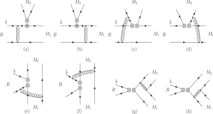
Figure 1: The Feynman diagrams of $B\rightarrow M_{1}M_{2}$ decays.

Due to the $\bra{\rho}V-A\ket{B}\bra{\eta_{q(s)}}V-A\ket{0}=-\bra{\rho}V-A\ket{B}\bra{\eta_{q(s)}}V+A\ket{0}$, the contribution of $(V-A)(V+A)$ operators is

$$F_{e\rho\eta_{q(s)}}^{R}=-F_{e\rho\eta_{q(s)}}.$$ (22)

The contribution of $(S+P)(S-P)$ operators which comes from Fierz transformation of $(V-A)(V+A)$ operators is

$$F_{e\rho\eta_{q(s)}}^{P}= i2\pi^{2}\dfrac{C_{F}}{N_{c}}f_{B}f_{\rho}^{||}f_{q(s)}m_{B}^{2}\int_{\xi_{u}}^{\xi_{d}}d\xi\int_{0}^{1}dx_{1}\int_{0}^{\infty}b_{1}db_{1}b_{3}db_{3}\int dk_{\perp}k_{\perp}(\dfrac{m_{B}}{2}+\dfrac{|\vec{k_{\perp}}|^{2}}{2\xi^{2}m_{B}})K(\vec{k})(E_{Q}+m_{Q})$$ (23)

$$\times J_{0}(k_{\perp}b_{3})\{\alpha_{s}(t_{e}^{1})[-2r_{\eta_{q(s)}}(E_{q}+k^{3})\phi_{\rho}(x_{1},b_{1})-2r_{\rho}r_{\eta_{q(s)}}r_{f}((x_{1}-3)E_{q}+(1-x_{1})k^{3})\phi_{\rho}^{s}(x_{1},b_{1})$$

$$-2r_{\rho}r_{\eta_{q(s)}}r_{f}((x_{1}-1)E_{q}-(x_{1}+1)k^{3})\phi_{\rho}^{t}(x_{1},b_{1})]h_{e}(\xi,1-x_{1},b_{3},b_{1})S_{t}(x_{1})exp[-S_{B}(t_{e}^{1})-S_{\rho}(t_{e}^{1})]$$

$$+\alpha_{s}(t_{e}^{2})[4r_{\rho}r_{\eta_{q(s)}}r_{f}(E_{q}-k^{3})\phi_{\rho}^{s}(x_{1},b_{1})]h_{e}(1-x_{1},\xi,b_{1},b_{3})S_{t}(\xi)exp[-S_{B}(t_{e}^{2})-S_{\rho}(t_{e}^{2})]\}.$$

The contributions of Figs. 1(c) and 1(d) are

$$M_{e\rho\eta_{q(s)}}= i2\pi^{2}\dfrac{C_{F}}{N_{c}}f_{B}f_{\rho}^{||}f_{q(s)}m_{B}^{2}\int_{\xi_{u}}^{\xi_{d}}d\xi\int_{0}^{1}dx_{1}dx_{2}\int_{0}^{\infty}b_{2}db_{2}b_{3}db_{3}\int dk_{\perp}k_{\perp}(\dfrac{m_{B}}{2}+\dfrac{|\vec{k_{\perp}}|^{2}}{2\xi^{2}m_{B}})K(\vec{k})(E_{Q}+m_{Q})$$ (24)

$$\times J_{0}(k_{\perp}b_{3})\{\alpha_{s}(t_{d}^{1})[x_{2}(E_{q}+k^{3})\phi_{\rho}(x_{1},b_{3})\phi_{\eta_{q(s)}}(x_{2},b_{2})-r_{\rho}r_{f}(x_{1}-1)(E_{q}-k^{3})(\phi_{\rho}^{s}(x_{1},b_{3})+\phi_{\rho}^{t}(x_{1},b_{3}))$$

$$\times\phi_{\eta_{q(s)}}(x_{2},b_{2})]h_{d}(\xi,x_{2},1-x_{1},b_{3},b_{2})exp[-S_{B}(t_{d}^{1})-S_{\rho}(t_{d}^{1})|_{b_{1}\rightarrow b_{3}}-S_{\eta_{q(s)}}(t_{d}^{1})]+\alpha_{s}(t_{d}^{2})[((x_{1}+x_{2}-2)E_{q}$$

$$+(x_{2}-x_{1})k^{3})\phi_{\rho}(x_{1},b_{3})\phi_{\eta_{q(s)}}(x_{2},b_{2})+r_{\rho}r_{f}(x_{1}-1)(E_{q}+k^{3})(\phi_{\rho}^{s}(x_{1},b_{3})-\phi_{\rho}^{t}(x_{1},b_{3}))\phi_{\eta_{q(s)}}(x_{2},b_{2})]$$

$$\times h_{d}(\xi,1-x_{2},1-x_{1},b_{3},b_{2})exp[-S_{B}(t_{d}^{2})-S_{\rho}(t_{d}^{2})|_{b_{1}\rightarrow b_{3}}-S_{\eta_{q(s)}}(t_{d}^{2})]\},$$

$$M_{e\rho\eta_{q(s)}}^{R}= i2\pi^{2}\dfrac{C_{F}}{N_{c}}f_{B}f_{\rho}^{||}f_{q(s)}m_{B}^{2}\int_{\xi_{u}}^{\xi_{d}}d\xi\int_{0}^{1}dx_{1}dx_{2}\int_{0}^{\infty}b_{2}db_{2}b_{3}db_{3}\int dk_{\perp}k_{\perp}(\dfrac{m_{B}}{2}+\dfrac{|\vec{k_{\perp}}|^{2}}{2\xi^{2}m_{B}})K(\vec{k})(E_{Q}+m_{Q})$$ (25)

$$\times J_{0}(k_{\perp}b_{3})\{\alpha_{s}(t_{d}^{1})[r_{\eta_{q(s)}}x_{2}(E_{q}+k^{3})\phi_{\rho}(x_{1},b_{3})(\dfrac{1}{6}\phi_{\sigma}^{\prime\eta_{q(s)}}(x_{2},b_{2})-\phi_{p}^{\eta_{q(s)}}(x_{2},b_{2}))+r_{\rho}r_{\eta_{q(s)}}r_{f}$$

$$\times((x_{1}+x_{2}-1)E_{q}-(x_{1}-x_{2}-1)k^{3})(\phi_{\rho}^{t}(x_{1},b_{3})\phi_{p}^{\eta_{q(s)}}(x_{2},b_{2})-\dfrac{1}{6}\phi_{\rho}^{s}(x_{1},b_{3})\phi_{\sigma}^{\prime\eta_{q(s)}}(x_{2},b_{2}))$$

$$+r_{\rho}r_{\eta_{q(s)}}r_{f}((x_{1}-x_{2}-1)E_{q}-(x_{1}+x_{2}-1)k^{3})(\dfrac{1}{6}\phi_{\rho}^{t}(x_{1},b_{3})\phi_{\sigma}^{\prime\eta_{q(s)}}(x_{2},b_{2})-\phi_{\rho}^{s}(x_{1},b_{3})$$

$$\times\phi_{p}^{\eta_{q(s)}}(x_{2},b_{2}))]h_{d}(\xi,x_{2},1-x_{1},b_{3},b_{2})exp[-S_{B}(t_{d}^{1})-S_{\rho}(t_{d}^{1})|_{b_{1}\rightarrow b_{3}}-S_{\eta_{q(s)}}(t_{d}^{1})]+\alpha_{s}(t_{d}^{2})$$

$$\times[-r_{\eta_{q(s)}}(x_{2}-1)(E_{q}+k^{3})\phi_{\rho}(x_{1},b_{3})(\phi_{p}^{\eta_{q(s)}}(x_{2},b_{2}))+\dfrac{1}{6}\phi_{\sigma}^{\prime\eta_{q(s)}}(x_{2},b_{2}))+r_{\rho}r_{\eta_{q(s)}}r_{f}((x_{1}+x_{2}-2)E_{q}$$

$$+(x_{2}-x_{1})k^{3})(\phi_{\rho}^{s}(x_{1},b_{3})\phi_{p}^{\eta_{q(s)}}(x_{2},b_{2})+\dfrac{1}{6}\phi_{\rho}^{t}(x_{1},b_{3})\phi_{\sigma}^{\prime\eta_{q(s)}}(x_{2},b_{2}))+r_{\rho}r_{\eta_{q(s)}}r_{f}((x_{2}-x_{1})E_{q}$$

$$+(x_{1}+x_{2}-2)k^{3})(\phi_{\rho}^{t}(x_{1},b_{3})\phi_{p}^{\eta_{q(s)}}(x_{2},b_{2})+\dfrac{1}{6}\phi_{\rho}^{s}(x_{1},b_{3})\phi_{\sigma}^{\prime\eta_{q(s)}}(x_{2},b_{2})]h_{d}(\xi,1-x_{2},1-x_{1},b_{3},b_{2})$$

$$\times exp[-S_{B}(t_{d}^{2})-S_{\rho}(t_{d}^{2})|_{b_{1}\rightarrow b_{3}}-S_{\eta_{q(s)}}(t_{d}^{2})]\},$$

$$M_{e\rho\eta_{q(s)}}^{P}= i2\pi^{2}\dfrac{C_{F}}{N_{c}}f_{B}f_{\rho}^{||}f_{q(s)}m_{B}^{2}\int_{\xi_{u}}^{\xi_{d}}d\xi\int_{0}^{1}dx_{1}dx_{2}\int_{0}^{\infty}b_{2}db_{2}b_{3}db_{3}\int dk_{\perp}k_{\perp}(\dfrac{m_{B}}{2}+\dfrac{|\vec{k_{\perp}}|^{2}}{2\xi^{2}m_{B}})K(\vec{k})(E_{Q}+m_{Q})$$ (26)

$$\times J_{0}(k_{\perp}b_{3})\{\alpha_{s}(t_{d}^{1})[((x_{1}-x_{2}-1)E_{q}-(x_{1}+x_{2}-1)k^{3})\phi_{\rho}(x_{1},b_{3})\phi_{\eta_{q(s)}}(x_{2},b_{2})+r_{\rho}r_{f}(x_{1}-1)$$

$$\times(E_{q}+k^{3})(\phi_{\rho}^{s}(x_{1},b_{3})-\phi_{\rho}^{t}(x_{1},b_{3}))\phi_{\eta_{q(s)}}(x_{2},b_{2})]h_{d}(\xi,x_{2},1-x_{1},b_{3},b_{2})exp[-S_{B}(t_{d}^{1})-S_{\rho}(t_{d}^{1})|_{b_{1}\rightarrow b_{3}}$$

$$-S_{\eta_{q(s)}}(t_{d}^{1})]+\alpha_{s}(t_{d}^{2})[-(x_{2}-1)(E_{q}+k^{3})\phi_{\rho}(x_{1},b_{3})\phi_{\eta_{q(s)}}(x_{2},b_{2})-r_{\rho}r_{f}(x_{1}-1)(E_{q}-k^{3})$$

$$\times(\phi_{\rho}^{s}(x_{1},b_{3})+\phi_{\rho}^{t}(x_{1},b_{3}))\phi_{\eta_{q(s)}}(x_{2},b_{2})]h_{d}(\xi,1-x_{2},1-x_{1},b_{3},b_{2})exp[-S_{B}(t_{d}^{2})-S_{\rho}(t_{d}^{2})|_{b_{1}\rightarrow b_{3}}$$

$$-S_{\eta_{q(s)}}(t_{d}^{2})]\}.$$

The amplitudes of Figs. 1(e) and 1(f) are

$$M_{a\rho\eta_{q(s)}}= i2\pi^{2}\dfrac{C_{F}}{N_{c}}f_{B}f_{\rho}^{||}f_{q(s)}m_{B}^{2}\int_{\xi_{u}}^{\xi_{d}}d\xi\int_{0}^{1}dx_{1}dx_{2}\int_{0}^{\infty}b_{2}db_{2}b_{3}db_{3}\int dk_{\perp}k_{\perp}(\dfrac{m_{B}}{2}+\dfrac{|\vec{k_{\perp}}|^{2}}{2\xi^{2}m_{B}})K(\vec{k})(E_{Q}+m_{Q})$$ (27)

$$\times J_{0}(k_{\perp}b_{3})\{\alpha_{s}(t_{f}^{1})[x_{1}(E_{q}-k^{3})\phi_{\rho}(x_{1},b_{2})\phi_{\eta_{q(s)}}(x_{2},b_{2})-r_{\rho}r_{\eta_{q(s)}}r_{f}((x_{1}-x_{2}+1)E_{q}$$

$$-(x_{1}+x_{2}-1)k^{3})(\dfrac{1}{6}\phi_{\rho}^{t}(x_{1},b_{2})\phi_{\sigma}^{\prime\eta_{q(s)}}(x_{2},b_{2})-\phi_{\rho}^{s}(x_{1},b_{2})\phi_{p}^{\eta_{q(s)}}(x_{2},b_{2}))-r_{\rho}r_{\eta_{q(s)}}r_{f}((x_{1}+x_{2}-1)E_{q}$$

$$-(x_{1}-x_{2}+1)k^{3})(\dfrac{1}{6}\phi_{\rho}^{s}(x_{1},b_{2})\phi_{\sigma}^{\prime\eta_{q(s)}}(x_{2},b_{2})-\phi_{\rho}^{t}(x_{1},b_{2})\phi_{p}^{\eta_{q(s)}}(x_{2},b_{2}))]h_{f}^{1}(1-x_{2},x_{1},b_{3},b_{2})$$

$$\times exp[-S_{B}(t_{f}^{1})-S_{\rho}(t_{f}^{1})|_{b_{1}\rightarrow b_{2}}-S_{\eta_{q(s)}}(t_{f}^{1})]+\alpha_{s}(t_{f}^{2})[(x_{2}-1)(E_{q}+k^{3})\phi_{\rho}(x_{1},b_{2})\phi_{\eta_{q(s)}}(x_{2},b_{2})$$

$$-r_{\rho}r_{\eta_{q(s)}}r_{f}((x_{1}-x_{2}+3)E_{q}-(x_{1}+x_{2}-1)k^{3})\phi_{\rho}^{s}(x_{1},b_{2})\phi_{p}^{\eta_{q(s)}}(x_{2},b_{2})+r_{\rho}r_{\eta_{q(s)}}r_{f}((x_{1}+x_{2}-1)E_{q}$$

$$-(x_{1}-x_{2}-1)k^{3})\phi_{\rho}^{t}(x_{1},b_{2})\phi_{p}^{\eta_{q(s)}}(x_{2},b_{2})-\dfrac{1}{6}r_{\rho}r_{\eta_{q(s)}}r_{f}((x_{1}+x_{2}-1)E_{q}-(x_{1}-x_{2}+3)k^{3})$$

$$\times\phi_{\rho}^{s}(x_{1},b_{2})\phi_{\sigma}^{\prime\eta_{q(s)}}(x_{2},b_{2})+\dfrac{1}{6}r_{\rho}r_{\eta_{q(s)}}r_{f}((x_{1}-x_{2}-1)E_{q}-(x_{1}+x_{2}-1)k^{3})\phi_{\rho}^{t}(x_{1},b_{2})\phi_{\sigma}^{\prime\eta_{q(s)}}(x_{2},b_{2})]$$

$$\times h_{f}^{2}(1-x_{2},x_{1},b_{3},b_{2})exp[-S_{B}(t_{f}^{2})-S_{\rho}(t_{f}^{2})|_{b_{1}\rightarrow b_{2}}-S_{\eta_{q(s)}}(t_{f}^{2})]\},$$

$$M_{a\rho\eta_{q(s)}}^{R}= i2\pi^{2}\dfrac{C_{F}}{N_{c}}f_{B}f_{\rho}^{||}f_{q(s)}m_{B}^{2}\int_{\xi_{u}}^{\xi_{d}}d\xi\int_{0}^{1}dx_{1}dx_{2}\int_{0}^{\infty}b_{2}db_{2}b_{3}db_{3}\int dk_{\perp}k_{\perp}(\dfrac{m_{B}}{2}+\dfrac{|\vec{k_{\perp}}|^{2}}{2\xi^{2}m_{B}})K(\vec{k})(E_{Q}+m_{Q})$$ (28)

$$\times J_{0}(k_{\perp}b_{3})\{\alpha_{s}(t_{f}^{1})[r_{\rho}r_{f}x_{1}(E_{q}+k_{3})(\phi_{\rho}^{s}(x_{1},b_{2})+\phi_{\rho}^{t}(x_{1},b_{2}))\phi_{\eta_{q(s)}}(x_{2},b_{2})+r_{\eta_{q(s)}}(x_{2}-1)(E_{q}-k^{3})$$

$$\times\phi_{\rho}(x_{1},b_{2})(\phi_{p}^{\eta_{q(s)}}(x_{2},b_{2})-\dfrac{1}{6}\phi_{\sigma}^{\prime\eta_{q(s)}}(x_{2},b_{2}))]h_{f}^{1}(1-x_{2},x_{1},b_{3},b_{2})exp[-S_{B}(t_{f}^{1})-S_{\rho}(t_{f}^{1})|_{b_{1}\rightarrow b_{2}}$$

$$-S_{\eta_{q(s)}}(t_{f}^{1})]+\alpha_{s}(t_{f}^{2})[-r_{\rho}r_{f}((x_{1}-2)E_{q}-x_{1}k^{3})(\phi_{\rho}^{s}(x_{1},b_{2})+\phi_{\rho}^{t}(x_{1},b_{2}))\phi_{\eta_{q(s)}}(x_{2},b_{2})$$

$$-r_{\eta_{q(s)}}((x_{2}+1)E_{q}+(x_{2}-1)k^{3})\phi_{\rho}(x_{1},b_{2})(\phi_{p}^{\eta_{q(s)}}(x_{2},b_{2})-\dfrac{1}{6}\phi_{\sigma}^{\prime\eta_{q(s)}}(x_{2},b_{2}))]h_{f}^{2}(1-x_{2},x_{1},b_{3},b_{2})$$

$$\times exp[-S_{B}(t_{f}^{2})-S_{\rho}(t_{f}^{2})|_{b_{1}\rightarrow b_{2}}-S_{\eta_{q(s)}}(t_{f}^{2})]\},$$

$$M_{a\rho\eta_{q(s)}}^{P}= i2\pi^{2}\dfrac{C_{F}}{N_{c}}f_{B}f_{\rho}^{||}f_{q(s)}m_{B}^{2}\int_{\xi_{u}}^{\xi_{d}}d\xi\int_{0}^{1}dx_{1}dx_{2}\int_{0}^{\infty}b_{2}db_{2}b_{3}db_{3}\int dk_{\perp}k_{\perp}(\dfrac{m_{B}}{2}+\dfrac{|\vec{k_{\perp}}|^{2}}{2\xi^{2}m_{B}})K(\vec{k})(E_{Q}+m_{Q})$$ (29)

$$\times J_{0}(k_{\perp}b_{3})\{\alpha_{s}(t_{f}^{1})[(x_{2}-1)(E_{q}+k^{3})\phi_{\rho}(x_{1},b_{2})\phi_{\eta_{q(s)}}(x_{2},b_{2})+r_{\rho}r_{\eta_{q(s)}}r_{f}((x_{1}+x_{2}-1)E_{q}$$

$$-(x_{1}-x_{2}+1)k^{3})(\phi_{\rho}^{t}(x_{1},b_{2})\phi_{p}^{\eta_{q(s)}}(x_{2},b_{2})-\dfrac{1}{6}\phi_{\rho}^{s}(x_{1},b_{2})\phi_{\sigma}^{\prime\eta_{q(s)}}(x_{2},b_{2}))+r_{\rho}r_{\eta_{q(s)}}r_{f}((x_{1}-x_{2}+1)E_{q}$$

$$-(x_{1}+x_{2}-1)k^{3})(\dfrac{1}{6}\phi_{\rho}^{t}(x_{1},b_{2})\phi_{\sigma}^{\prime\eta_{q(s)}}(x_{2},b_{2})-\phi_{\rho}^{s}(x_{1},b_{2})\phi_{p}^{\eta_{q(s)}}(x_{2},b_{2}))]h_{f}^{1}(1-x_{2},x_{1},b_{3},b_{2})$$

$$\times exp[-S_{B}(t_{f}^{1})-S_{\rho}(t_{f}^{1})|_{b_{1}\rightarrow b_{2}}-S_{\eta_{q(s)}}(t_{f}^{1})]+\alpha_{s}(t_{f}^{2})[x_{1}(E_{q}-k^{3})\phi_{\rho}(x_{1},b_{2})\phi_{\eta_{q(s)}}(x_{2},b_{2})$$

$$+r_{\rho}r_{\eta_{q(s)}}r_{f}((x_{1}-x_{2}+3)E_{q}-(x_{1}+x_{2}-1)k^{3})\phi_{\rho}^{s}(x_{1},b_{2})\phi_{p}^{\eta_{q(s)}}(x_{2},b_{2})+r_{\rho}r_{\eta_{q(s)}}r_{f}((x_{1}+x_{2}-1)E_{q}$$

$$-(x_{1}-x_{2}+3)k^{3})\phi_{\rho}^{t}(x_{1},b_{2})\phi_{p}^{\eta_{q(s)}}(x_{2},b_{2})-\dfrac{1}{6}r_{\rho}r_{\eta_{q(s)}}r_{f}((x_{1}+x_{2}-1)E_{q}-(x_{1}-x_{2}-1)k^{3})\phi_{\rho}^{s}(x_{1},b_{2})$$

$$\times\phi_{\sigma}^{\prime\eta_{q(s)}}(x_{2},b_{2})-\dfrac{1}{6}r_{\rho}r_{\eta_{q(s)}}r_{f}((x_{1}-x_{2}-1)E_{q}-(x_{1}+x_{2}-1)k^{3})\phi_{\rho}^{t}(x_{1},b_{2})\phi_{\sigma}^{\prime\eta_{q(s)}}(x_{2},b_{2})]$$

$$\times h_{f}^{2}(1-x_{2},x_{1},b_{3},b_{2})exp[-S_{B}(t_{f}^{2})-S_{\rho}(t_{f}^{2})|_{b_{1}\rightarrow b_{2}}-S_{\eta_{q(s)}}(t_{f}^{2})]\}.$$

If $M_{1}$ is $\eta^{(\prime)}$ meson, then Figs. 1(a) and 1(b) contribute to $B\rightarrow\eta_{q(s)}$ form factor. The corresponding amplitude contributed by Figs. 1(a) and 1(b) with the insertion of operators of $(V-A)(V-A)$ is

$$F_{e\eta_{q(s)}\rho}= i2\pi^{2}\dfrac{C_{F}}{N_{c}}f_{B}f_{\rho}^{||}f_{q(s)}m_{B}^{2}\int_{\xi_{u}}^{\xi_{d}}d\xi\int_{0}^{1}dx_{1}\int_{0}^{\infty}b_{1}db_{1}b_{3}db_{3}\int dk_{\perp}k_{\perp}(\dfrac{m_{B}}{2}+\dfrac{|\vec{k_{\perp}}|^{2}}{2\xi^{2}m_{B}})K(\vec{k})(E_{Q}+m_{Q})$$ (30)

$$\times J_{0}(k_{\perp}b_{3})\{\alpha_{s}(t_{e}^{1})[-((x_{1}-2)E_{q}-x_{1}k^{3})\phi_{\eta_{q(s)}}(x_{1},b_{1})+r_{\eta_{q(s)}}((1-2x_{1})E_{q}+k^{3})(\dfrac{1}{6}\phi_{\sigma}^{\prime\eta_{q(s)}}(x_{1},b_{1})$$

$$-\phi_{p}^{\eta_{q(s)}}(x_{1},b_{1}))]h_{e}(\xi,1-x_{1},b_{3},b_{1})S_{t}(x_{1})exp[-S_{B}(t_{e}^{1})-S_{\eta_{q(s)}}(t_{e}^{1})]+\alpha_{s}(t_{e}^{2})[2r_{\eta_{q(s)}}(E_{q}-k^{3})$$

$$\times\phi_{p}^{\eta_{q(s)}}(x_{1},b_{1})]h_{e}(1-x_{1},\xi,b_{1},b_{3})S_{t}(\xi)exp[-S_{B}(t_{e}^{2})-S_{\eta_{q(s)}}(t_{e}^{2})]\},$$

Due to the relation $\bra{\eta_{q(s)}}V-A\ket{B}\bra{\rho}V-A\ket{0}=\bra{\eta_{q(s)}}V-A\ket{B}\bra{\rho}V+A\ket{0}$, the contribution of $(V-A)(V+A)$ operators is

$$F_{e\eta_{q(s)}\rho}^{R}=F_{e\eta_{q(s)}\rho}.$$ (31)

The contribution of $(S+P)(S-P)$ operators is $F_{e\eta_{q(s)\rho}}^{P}=0$ on account of $\bra{\rho}S+P\ket{0}=0$.

Similarly, the contributions of Figs. 1(c) and 1(d) are

$$M_{e\eta_{q(s)}\rho}= i2\pi^{2}\dfrac{C_{F}}{N_{c}}f_{B}f_{\rho}^{||}f_{q(s)}m_{B}^{2}\int_{\xi_{u}}^{\xi_{d}}d\xi\int_{0}^{1}dx_{1}dx_{2}\int_{0}^{\infty}b_{2}db_{2}b_{3}db_{3}\int dk_{\perp}k_{\perp}(\dfrac{m_{B}}{2}+\dfrac{|\vec{k_{\perp}}|^{2}}{2\xi^{2}m_{B}})K(\vec{k})(E_{Q}+m_{Q})$$ (32)

$$\times J_{0}(k_{\perp}b_{3})\{\alpha_{s}(t_{d}^{1})[x_{2}(E_{q}+k^{3})\phi_{\eta_{q(s)}}(x_{1},b_{3})\phi_{\rho}(x_{2},b_{2})+r_{\eta_{q(s)}}(x_{1}-1)(E_{q}-k^{3})(\phi_{p}^{\eta_{q(s)}}(x_{1},b_{3})$$

$$+\dfrac{1}{6}\phi_{\sigma}^{\prime\eta_{q(s)}}(x_{1},b_{3}))\phi_{\rho}(x_{2},b_{2})]h_{d}(\xi,x_{2},1-x_{1},b_{3},b_{2})exp[-S_{B}(t_{d}^{1})-S_{\rho}(t_{d}^{1})-S_{\eta_{q(s)}}(t_{d}^{1})|_{b_{1}\rightarrow b_{3}}]$$

$$+\alpha_{s}(t_{d}^{2})[((x_{1}+x_{2}-2)E_{q}+(x_{2}-x_{1})k^{3})\phi_{\eta_{q(s)}}(x_{1},b_{3})\phi_{\rho}(x_{2},b_{2})-r_{\eta_{q(s)}}(x_{1}-1)(E_{q}+k^{3})$$

$$\times(\phi_{p}^{\eta_{q(s)}}(x_{1},b_{3})-\dfrac{1}{6}\phi_{\sigma}^{\prime\eta_{q(s)}}(x_{1},b_{3}))\phi_{\rho}(x_{2},b_{2})]h_{d}(\xi,1-x_{2},1-x_{1},b_{3},b_{2})$$

$$\times exp[-S_{B}(t_{d}^{2})-S_{\rho}(t_{d}^{2})-S_{\eta_{q(s)}}(t_{d}^{2})|_{b_{1}\rightarrow b_{3}}]\},$$

$$M_{e\eta_{q(s)}\rho}^{R}= i2\pi^{2}\dfrac{C_{F}}{N_{c}}f_{B}f_{\rho}^{||}f_{q(s)}m_{B}^{2}\int_{\xi_{u}}^{\xi_{d}}d\xi\int_{0}^{1}dx_{1}dx_{2}\int_{0}^{\infty}b_{2}db_{2}b_{3}db_{3}\int dk_{\perp}k_{\perp}(\dfrac{m_{B}}{2}+\dfrac{|\vec{k_{\perp}}|^{2}}{2\xi^{2}m_{B}})K(\vec{k})(E_{Q}+m_{Q})$$ (33)

$$\times J_{0}(k_{\perp}b_{3})\{\alpha_{s}(t_{d}^{1})[-r_{\rho}r_{f}x_{2}(E_{q}+k^{3})\phi_{\eta_{q(s)}}(x_{1},b_{3})(\phi_{\rho}^{s}(x_{2},b_{2})-\phi_{\rho}^{t}(x_{2},b_{2}))+r_{\rho}r_{\eta_{q(s)}}r_{f}((x_{1}+x_{2}-1)E_{q}$$

$$-(x_{1}-x_{2}-1)k^{3})(\phi_{p}^{\eta_{q(s)}}(x_{1},b_{3})\phi_{\rho}^{t}(x_{2},b_{2})-\dfrac{1}{6}\phi_{\sigma}^{\prime\eta_{q(s)}}(x_{1},b_{3})\phi_{\rho}^{s}(x_{2},b_{2}))+r_{\rho}r_{\eta_{q(s)}}r_{f}((x_{1}-x_{2}-1)E_{q}$$

$$-(x_{1}+x_{2}-1)k^{3})(\phi_{p}^{\eta_{q(s)}}(x_{1},b_{3})\phi_{\rho}^{s}(x_{2},b_{2})-\dfrac{1}{6}\phi_{\sigma}^{\prime\eta_{q(s)}}(x_{1},b_{3})\phi_{\rho}^{t}(x_{2},b_{2}))]h_{d}(\xi,x_{2},1-x_{1},b_{3},b_{2})$$

$$\times exp[-S_{B}(t_{d}^{1})-S_{\rho}(t_{d}^{1})-S_{\eta_{q(s)}}(t_{d}^{1})|_{b_{1}\rightarrow b_{3}}]+\alpha_{s}(t_{d}^{2})[-r_{\rho}r_{f}(x_{2}-1)(E_{q}+k^{3})\phi_{\eta_{q(s)}}(x_{1},b_{3})(\phi_{\rho}^{s}(x_{2},b_{2}))$$

$$+\phi_{\rho}^{t}(x_{2},b_{2}))-r_{\rho}r_{\eta_{q(s)}}r_{f}((x_{1}+x_{2}-2)E_{q}+(x_{2}-x_{1})k^{3})(\phi_{p}^{\eta_{q(s)}}(x_{1},b_{3})\phi_{\rho}^{s}(x_{2},b_{2})$$

$$+\dfrac{1}{6}\phi_{\sigma}^{\prime\eta_{q(s)}}(x_{1},b_{3})\phi_{\rho}^{t}(x_{2},b_{2})-r_{\rho}r_{\eta_{q(s)}}r_{f}((x_{2}-x_{1})E_{q}+(x_{1}+x_{2}-2)k^{3})(\phi_{p}^{\eta_{q(s)}}(x_{1},b_{3})\phi_{\rho}^{t}(x_{2},b_{2})$$

$$+\dfrac{1}{6}\phi_{\sigma}^{\prime\eta_{q(s)}}(x_{1},b_{3})\phi_{\rho}^{s}(x_{2},b_{2})]h_{d}(\xi,1-x_{2},1-x_{1},b_{3},b_{2})exp[-S_{B}(t_{d}^{2})-S_{\rho}(t_{d}^{2})-S_{\eta_{q(s)}}(t_{d}^{2})|_{b_{1}\rightarrow b_{3}}]\},$$

$$M_{e\eta_{q(s)}\rho}^{P}= i2\pi^{2}\dfrac{C_{F}}{N_{c}}f_{B}f_{\rho}^{||}f_{q(s)}m_{B}^{2}\int_{\xi_{u}}^{\xi_{d}}d\xi\int_{0}^{1}dx_{1}dx_{2}\int_{0}^{\infty}b_{2}db_{2}b_{3}db_{3}\int dk_{\perp}k_{\perp}(\dfrac{m_{B}}{2}+\dfrac{|\vec{k_{\perp}}|^{2}}{2\xi^{2}m_{B}})K(\vec{k})(E_{Q}+m_{Q})$$ (34)

$$\times J_{0}(k_{\perp}b_{3})\{\alpha_{s}(t_{d}^{1})[-((x_{1}-x_{2}-1)E_{q}-(x_{1}+x_{2}-1)k^{3})\phi_{\eta_{q(s)}}(x_{1},b_{3})\phi_{\rho}(x_{2},b_{2})-r_{\eta_{q(s)}}(x_{1}-1)$$

$$\times(E_{q}+k^{3})(\dfrac{1}{6}\phi_{\sigma}^{\prime\eta_{q(s)}}(x_{1},b_{3})-\phi_{p}^{\eta_{q(s)}}(x_{1},b_{3}))\phi_{\rho}(x_{2},b_{2})]h_{d}(\xi,x_{2},1-x_{1},b_{3},b_{2})$$

$$\times exp[-S_{B}(t_{d}^{1})-S_{\rho}(t_{d}^{1})-S_{\eta_{q(s)}}(t_{d}^{1})|_{b_{1}\rightarrow b_{3}}]+\alpha_{s}(t_{d}^{2})[(x_{2}-1)(E_{q}+k^{3})\phi_{\eta_{q(s)}}(x_{1},b_{3})\phi_{\rho}(x_{2},b_{2})$$

$$-r_{\eta_{q(s)}}(x_{1}-1)(E_{q}-k^{3})(\phi_{p}^{\eta_{q(s)}}(x_{1},b_{3})+\dfrac{1}{6}\phi_{\sigma}^{\prime\eta_{q(s)}}(x_{1},b_{3}))\phi_{\rho}(x_{2},b_{2})]h_{d}(\xi,1-x_{2},1-x_{1},b_{3},b_{2})$$

$$\times exp[-S_{B}(t_{d}^{2})-S_{\rho}(t_{d}^{2})-S_{\eta_{q(s)}}(t_{d}^{2})|_{b_{1}\rightarrow b_{3}}]\}.$$

The amplitudes of Figs. 1(e) and 1(f) are

$$M_{a\eta_{q(s)}\rho}= i2\pi^{2}\dfrac{C_{F}}{N_{c}}f_{B}f_{\rho}^{||}f_{q(s)}m_{B}^{2}\int_{\xi_{u}}^{\xi_{d}}d\xi\int_{0}^{1}dx_{1}dx_{2}\int_{0}^{\infty}b_{2}db_{2}b_{3}db_{3}\int dk_{\perp}k_{\perp}(\dfrac{m_{B}}{2}+\dfrac{|\vec{k_{\perp}}|^{2}}{2\xi^{2}m_{B}})K(\vec{k})(E_{Q}+m_{Q})$$ (35)

$$\times J_{0}(k_{\perp}b_{3})\{\alpha_{s}(t_{f}^{1})[x_{1}(E_{q}-k^{3})\phi_{\eta_{q(s)}}(x_{1},b_{2})\phi_{\rho}(x_{2},b_{2})-r_{\rho}r_{\eta_{q(s)}}r_{f}((x_{1}-x_{2}+1)E_{q}$$

$$-(x_{1}+x_{2}-1)k^{3})(\phi_{p}^{\eta_{q(s)}}(x_{1},b_{2})\phi_{\rho}^{s}(x_{2},b_{2})-\dfrac{1}{6}\phi_{\sigma}^{\prime\eta_{q(s)}}(x_{1},b_{2})\phi_{\rho}^{t}(x_{2},b_{2}))-r_{\rho}r_{\eta_{q(s)}}r_{f}((x_{1}+x_{2}-1)E_{q}$$

$$-(x_{1}-x_{2}+1)k^{3})(\dfrac{1}{6}\phi_{\sigma}^{\prime\eta_{q(s)}}(x_{1},b_{2})\phi_{\rho}^{s}(x_{2},b_{2})-\phi_{p}^{\eta_{q(s)}}(x_{1},b_{2})\phi_{\rho}^{t}(x_{2},b_{2}))]h_{f}^{1}(1-x_{2},x_{1},b_{3},b_{2})$$

$$\times exp[-S_{B}(t_{f}^{1})-S_{\rho}(t_{f}^{1})-S_{\eta_{q(s)}}(t_{f}^{1})|_{b_{1}\rightarrow b_{2}}]+\alpha_{s}(t_{f}^{2})[(x_{2}-1)(E_{q}+k^{3})\phi_{\eta_{q(s)}}(x_{1},b_{2})\phi_{\rho}(x_{2},b_{2})$$

$$+r_{\rho}r_{\eta_{q(s)}}r_{f}((x_{1}-x_{2}+3)E_{q}-(x_{1}+x_{2}-1)k^{3})\phi_{p}^{\eta_{q(s)}}(x_{1},b_{2})\phi_{\rho}^{s}(x_{2},b_{2})+r_{\rho}r_{\eta_{q(s)}}r_{f}((x_{1}+x_{2}-1)E_{q}$$

$$-(x_{1}-x_{2}+3)k^{3})\phi_{p}^{\eta_{q(s)}}(x_{1},b_{2})\phi_{\rho}^{t}(x_{2},b_{2})-\dfrac{1}{6}r_{\rho}r_{\eta_{q(s)}}r_{f}((x_{1}+x_{2}-1)E_{q}-(x_{1}-x_{2}-1)k^{3})$$

$$\times\phi_{\sigma}^{\prime\eta_{q(s)}}(x_{1},b_{2})\phi_{\rho}^{s}(x_{2},b_{2})-\dfrac{1}{6}r_{\rho}r_{\eta_{q(s)}}r_{f}((x_{1}-x_{2}-1)E_{q}-(x_{1}+x_{2}-1)k^{3})$$

$$\times\phi_{\sigma}^{\prime\eta_{q(s)}}(x_{1},b_{2})\phi_{\rho}^{t}(x_{2},b_{2})]h_{f}^{2}(1-x_{2},x_{1},b_{3},b_{2})exp[-S_{B}(t_{f}^{2})-S_{\rho}(t_{f}^{2})-S_{\eta_{q(s)}}(t_{f}^{2})|_{b_{1}\rightarrow b_{2}}]\},$$

$$M_{a\eta_{q(s)}\rho}^{R}= i2\pi^{2}\dfrac{C_{F}}{N_{c}}f_{B}f_{\rho}^{||}f_{q(s)}m_{B}^{2}\int_{\xi_{u}}^{\xi_{d}}d\xi\int_{0}^{1}dx_{1}dx_{2}\int_{0}^{\infty}b_{2}db_{2}b_{3}db_{3}\int dk_{\perp}k_{\perp}(\dfrac{m_{B}}{2}+\dfrac{|\vec{k_{\perp}}|^{2}}{2\xi^{2}m_{B}})K(\vec{k})(E_{Q}+m_{Q})$$ (36)

$$\times J_{0}(k_{\perp}b_{3})\{\alpha_{s}(t_{f}^{1})[-r_{\eta_{q(s)}}x_{1}(E_{q}+k_{3})(\phi_{p}^{\eta_{q(s)}}(x_{1},b_{2})+\dfrac{1}{6}\phi_{\sigma}^{\prime\eta_{q(s)}}(x_{1},b_{2}))\phi_{\rho}(x_{2},b_{2})+r_{\rho}r_{f}(x_{2}-1)$$

$$\times(E_{q}-k^{3})\phi_{\eta_{q(s)}}(x_{1},b_{2})(\phi_{\rho}^{s}(x_{2},b_{2})-\phi_{\rho}^{t}(x_{2},b_{2}))]h_{f}^{1}(1-x_{2},x_{1},b_{3},b_{2})exp[-S_{B}(t_{f}^{1})-S_{\rho}(t_{f}^{1})$$

$$-S_{\eta_{q(s)}}(t_{f}^{1})|_{b_{1}\rightarrow b_{2}}]+\alpha_{s}(t_{f}^{2})[r_{\eta_{q(s)}}((x_{1}-2)E_{q}-x_{1}k^{3})(\phi_{p}^{\eta_{q(s)}}(x_{1},b_{2})+\dfrac{1}{6}\phi_{\sigma}^{\prime\eta_{q(s)}}(x_{1},b_{2}))\phi_{\rho}(x_{2},b_{2})$$

$$-r_{\rho}r_{f}((x_{2}+1)E_{q}+(x_{2}-1)k^{3})\phi_{\eta_{q(s)}}(x_{1},b_{2})(\phi_{\rho}^{s}(x_{2},b_{2})-\phi_{\rho}^{t}(x_{2},b_{2}))]h_{f}^{2}(1-x_{2},x_{1},b_{3},b_{2})$$

$$\times exp[-S_{B}(t_{f}^{2})-S_{\rho}(t_{f}^{2})-S_{\eta_{q(s)}}(t_{f}^{2})|_{b_{1}\rightarrow b_{2}}]\},$$

$$M_{a\eta_{q(s)}\rho}^{P}= i2\pi^{2}\dfrac{C_{F}}{N_{c}}f_{B}f_{\rho}^{||}f_{q(s)}m_{B}^{2}\int_{\xi_{u}}^{\xi_{d}}d\xi\int_{0}^{1}dx_{1}dx_{2}\int_{0}^{\infty}b_{2}db_{2}b_{3}db_{3}\int dk_{\perp}k_{\perp}(\dfrac{m_{B}}{2}+\dfrac{|\vec{k_{\perp}}|^{2}}{2\xi^{2}m_{B}})K(\vec{k})(E_{Q}+m_{Q})$$ (37)

$$\times J_{0}(k_{\perp}b_{3})\{\alpha_{s}(t_{f}^{1})[(x_{2}-1)(E_{q}+k^{3})\phi_{\eta_{q(s)}}(x_{1},b_{2})\phi_{\rho}(x_{2},b_{2})+r_{\rho}r_{\eta_{q(s)}}r_{f}((x_{1}+x_{2}-1)E_{q}$$

$$-(x_{1}-x_{2}+1)k^{3})(\phi_{p}^{\eta_{q(s)}}(x_{1},b_{2})\phi_{\rho}^{t}(x_{2},b_{2})-\dfrac{1}{6}\phi_{\sigma}^{\prime\eta_{q(s)}}(x_{1},b_{2})\phi_{\rho}^{s}(x_{2},b_{2}))+r_{\rho}r_{\eta_{q(s)}}r_{f}((x_{1}-x_{2}+1)E_{q}$$

$$-(x_{1}+x_{2}-1)k^{3})(\phi_{p}^{\eta_{q(s)}}(x_{1},b_{2})\phi_{\rho}^{s}(x_{2},b_{2})-\dfrac{1}{6}\phi_{\sigma}^{\prime\eta_{q(s)}}(x_{1},b_{2})\phi_{\rho}^{t}(x_{2},b_{2}))]h_{f}^{1}(1-x_{2},x_{1},b_{3},b_{2})$$

$$\times exp[-S_{B}(t_{f}^{1})-S_{\rho}(t_{f}^{1})-S_{\eta_{q(s)}}(t_{f}^{1})|_{b_{1}\rightarrow b_{2}}]+\alpha_{s}(t_{f}^{2})[x_{1}(E_{q}-k^{3})\phi_{\eta_{q(s)}}(x_{1},b_{2})\phi_{\rho}(x_{2},b_{2})$$

$$-r_{\rho}r_{\eta_{q(s)}}r_{f}((x_{1}-x_{2}+3)E_{q}-(x_{1}+x_{2}-1)k^{3})\phi_{p}^{\eta_{q(s)}}(x_{1},b_{2})\phi_{\rho}^{s}(x_{2},b_{2})+r_{\rho}r_{\eta_{q(s)}}r_{f}$$

$$\times((x_{1}+x_{2}-1)E_{q}-(x_{1}-x_{2}-1)k^{3})\phi_{p}^{\eta_{q(s)}}(x_{1},b_{2})\phi_{\rho}^{t}(x_{2},b_{2})-\dfrac{1}{6}r_{\rho}r_{\eta_{q(s)}}r_{f}((x_{1}+x_{2}-1)E_{q}$$

$$-(x_{1}-x_{2}+3)k^{3})\phi_{\sigma}^{\prime\eta_{q(s)}}(x_{1},b_{2})\phi_{\rho}^{s}(x_{2},b_{2})+\dfrac{1}{6}r_{\rho}r_{\eta_{q(s)}}r_{f}((x_{1}-x_{2}-1)E_{q}-(x_{1}+x_{2}-1)k^{3})$$

$$\times\phi_{\sigma}^{\prime\eta_{q(s)}}(x_{1},b_{2})\phi_{\rho}^{t}(x_{2},b_{2})]h_{f}^{2}(1-x_{2},x_{1},b_{3},b_{2})exp[-S_{B}(t_{f}^{2})-S_{\rho}(t_{f}^{2})-S_{\eta_{q(s)}}(t_{f}^{2})|_{b_{1}\rightarrow b_{2}}]\}.$$

Particularly, there are no contributions from Figs. 1(g) and 1(h) in the decay modes of $B\rightarrow\rho\eta^{(\prime)}$. In Eqs. (21)$-$(37) we have defined $N_{c}=3$, $C_{F}=4/3$, $r_{\eta_{q(s)}}=\mu_{\eta_{q(s)}}/m_{B}$ and $r_{\rho}=m_{\rho}/m_{B}$. The exponential $\exp[-S_{B,\rho,\eta_{q(s)}}(t)]$ is the Sudakov factors and $S_{t}(x)$ the threshold factor which are given in Appendix A. The functions $h_{i}$’s are given as

$$h_{e}(x_{1},x_{2},b_{1},b_{2}) = K_{0}(\sqrt{x_{1}x_{2}}m_{B}b_{1})[\theta(b_{1}-b_{2})I_{0}(\sqrt{x_{2}}m_{B}b_{2})K_{0}(\sqrt{x_{2}}m_{B}b_{1})$$

$$+\theta(b_{2}-b_{1})I_{0}(\sqrt{x_{2}}m_{B}b_{1})K_{0}(\sqrt{x_{2}}m_{B}b_{2})],$$

$$h_{a}(x_{1},x_{2},b_{1},b_{2}) = K_{0}(-i\sqrt{x_{1}x_{2}}m_{B}b_{1})[\theta(b_{1}-b_{2})I_{0}(-i\sqrt{x_{2}}m_{B}b_{2})K_{0}(-i\sqrt{x_{2}}m_{B}b_{1})$$

$$+\theta(b_{2}-b_{1})I_{0}(-i\sqrt{x_{2}}m_{B}b_{1})K_{0}(-i\sqrt{x_{2}}m_{B}b_{2})],$$

$$h_{d}(x_{1},x_{2},x_{3},b_{1},b_{2}) = K_{0}(-i\sqrt{x_{2}x_{3}}m_{B}b_{2})[\theta(b_{1}-b_{2})I_{0}(\sqrt{x_{1}x_{3}}m_{B}b_{2})K_{0}(\sqrt{x_{1}x_{3}}m_{B}b_{1})$$

$$+\theta(b_{2}-b_{1})I_{0}(\sqrt{x_{1}x_{3}}m_{B}b_{1})K_{0}(\sqrt{x_{1}x_{3}}m_{B}b_{2})],$$

$$h_{f}^{1}(x_{1},x_{2},b_{1},b_{2}) = K_{0}(-i\sqrt{x_{1}x_{2}}m_{B}b_{1})[\theta(b_{1}-b_{2})I_{0}(-i\sqrt{x_{1}x_{2}}m_{B}b_{2})K_{0}(-i\sqrt{x_{1}x_{2}}m_{B}b_{1})$$

$$+\theta(b_{2}-b_{1})I_{0}(-i\sqrt{x_{1}x_{2}}m_{B}b_{1})K_{0}(-i\sqrt{x_{1}x_{2}}m_{B}b_{2})],$$

$$h_{f}^{2}(x_{1},x_{2},b_{1},b_{2}) = K_{0}(\sqrt{x_{1}+x_{2}-x_{1}x_{2}}m_{B}b_{1})[\theta(b_{1}-b_{2})I_{0}(-i\sqrt{x_{1}x_{2}}m_{B}b_{2})K_{0}(-i\sqrt{x_{1}x_{2}}m_{B}b_{1})$$

$$+\theta(b_{2}-b_{1})I_{0}(-i\sqrt{x_{1}x_{2}}m_{B}b_{1})K_{0}(-i\sqrt{x_{1}x_{2}}m_{B}b_{2})].$$

In order to suppress the large logarithmic terms in higher-order corrections, the hard scales are tanke as the maximum mass scales in the amplitudes

$$t_{e}^{1} = max(\sqrt{1-x_{1}}m_{B},1/b_{3},1/b_{1}),$$

$$t_{e}^{2} = max(\sqrt{\xi}m_{B},1/b_{3},1/b_{1}),$$

$$t_{a}^{1} = max(\sqrt{x_{1}}m_{B},1/b_{1},1/b_{2}),$$

$$t_{a}^{2} = max(\sqrt{1-x_{2}}m_{B},1/b_{1},1/b_{2}),$$

$$t_{d}^{1} = max(\sqrt{(1-x_{1})x_{2}}m_{B},\sqrt{(1-x_{1})\xi}m_{B},1/b_{3},1/b_{2}),$$

$$t_{d}^{2} = max(\sqrt{(1-x_{1})(1-x_{2})}m_{B},\sqrt{(1-x_{1})\xi}m_{B},1/b_{3},1/b_{2}),$$

$$t_{f}^{1} = max(\sqrt{x_{1}(1-x_{2})}m_{B},1/b_{3},1/b_{2}),$$

$$t_{f}^{2} = max(\sqrt{x_{1}(1-x_{2})}m_{B},\sqrt{x_{1}+(1-x_{2})-x_{1}(1-x_{2})}m_{B},1/b_{3},1/b_{2}).$$ (43)

The decay amplitudes of the $B\rightarrow\rho\eta^{(\prime)}$ can be written as

$$\sqrt{2}\mathcal{M}(B^{-}\rightarrow\rho^{-}\eta_{q}) = \{V_{u}(C_{1}+\dfrac{C_{2}}{N_{c}})-V_{t}[(2+\dfrac{1}{N_{c}})C_{3}+(1+\dfrac{2}{N_{c}})C_{4}\ +(1-\dfrac{1}{N_{c}})\dfrac{1}{2}C_{9}-(1-\dfrac{1}{N_{c}})\dfrac{1}{2}C_{10}]\}F_{e\rho\eta_{q}}$$ (44)

$$-V_{t}(2C_{5}+2\dfrac{C_{6}}{N_{c}}+\dfrac{1}{2}C_{7}+\dfrac{1}{2}\dfrac{C_{8}}{N_{c}})F_{e\rho\eta_{q}}^{R}-V_{t}(\dfrac{C_{5}}{N_{c}}+C_{6}-\dfrac{1}{2}\dfrac{C_{7}}{N_{c}}-\dfrac{1}{2}C_{8})F_{e\rho\eta_{q}}^{P}$$

$$+[V_{u}(\dfrac{C_{1}}{N_{c}}+C_{2})-V_{t}(\dfrac{C_{3}}{N_{c}}+C_{4}+\dfrac{C_{9}}{N_{c}}+C_{10})]F_{e\eta_{q}\rho}-V_{t}(\dfrac{C_{5}}{N_{c}}+C_{6}+\dfrac{C_{7}}{N_{c}}+C_{8})F_{e\eta_{q}\rho}^{P}$$

$$+[V_{u}\dfrac{C_{2}}{N_{c}}-V_{t}\dfrac{1}{N_{c}}(C_{3}+2C_{4}-\dfrac{1}{2}C_{9}+\dfrac{1}{2}C_{10})]M_{e\rho\eta_{q}}-V_{t}\dfrac{1}{N_{c}}(C_{5}-\dfrac{1}{2}C_{7})M_{e\rho\eta_{q}}^{R}$$

$$-V_{t}\dfrac{1}{N_{c}}(2C_{6}+\dfrac{1}{2}C_{8})M_{e\rho\eta_{q}}^{P}+[V_{u}\dfrac{C_{1}}{N_{c}}-V_{t}\dfrac{1}{N_{c}}(C_{3}+C_{9})](M_{e\eta_{q}\rho}+M_{a\rho\eta_{q}}+M_{a\eta_{q}\rho})$$

$$-V_{t}\dfrac{1}{N_{c}}(C_{5}+C_{7})(M_{e\eta_{q}\rho}^{R}+M_{a\rho\eta_{q}}^{R}+M_{a\eta_{q}\rho}^{R}),$$

$$\mathcal{M}(B^{-}\rightarrow\rho^{-}\eta_{s}) = -V_{t}(C_{3}+\dfrac{C_{4}}{N_{c}}-\dfrac{1}{2}C_{9}-\dfrac{1}{2}\dfrac{C_{10}}{N_{c}})F_{e\rho\eta_{s}}-V_{t}(C_{5}+\dfrac{C_{6}}{N_{c}}-\dfrac{1}{2}C_{7}-\dfrac{1}{2}\dfrac{C_{8}}{N_{c}})F_{e\rho\eta_{s}}^{R}$$ (45)

$$-V_{t}\dfrac{1}{N_{c}}(C_{4}-\dfrac{1}{2}C_{10})M_{e\rho\eta_{s}}-V_{t}\dfrac{1}{N_{c}}(C_{6}-\dfrac{1}{2}C_{8})M_{e\rho\eta_{s}}^{P}.$$

$$2\mathcal{M}(\bar{B^{0}}\rightarrow\rho^{0}\eta_{q}) = -\{V_{u}(C_{1}+\dfrac{C_{2}}{N_{c}})-V_{t}[(2+\dfrac{1}{N_{c}})C_{3}+(1+\dfrac{2}{N_{c}})C_{4}+(1-\dfrac{1}{N_{c}})\dfrac{1}{2}C_{9}-(1-\dfrac{1}{N_{c}})\dfrac{1}{2}C_{10}]\}F_{e\rho\eta_{q}}$$ (46)

$$+\{V_{u}(C_{1}+\dfrac{C_{2}}{N_{c}})-V_{t}[-\dfrac{C_{3}}{N_{c}}-C_{4}+(3+\dfrac{1}{N_{c}})\dfrac{1}{2}C_{9}+(1+\dfrac{3}{N_{c}})\dfrac{1}{2}C_{10}]\}F_{e\eta_{q}\rho}$$

$$+V_{t}(2C_{5}+2\dfrac{C_{6}}{N_{c}}+\dfrac{1}{2}C_{7}+\dfrac{1}{2}\dfrac{C_{8}}{N_{c}})F_{e\rho\eta_{q}}^{R}-V_{t}(\dfrac{3}{2}C_{7}+\dfrac{3}{2}\dfrac{C_{8}}{N_{c}})F_{e\eta_{q}\rho}^{R}$$

$$+V_{t}(\dfrac{C_{5}}{N_{c}}+C_{6}-\dfrac{1}{2}\dfrac{C_{7}}{N_{c}}-\dfrac{1}{2}C_{8})(F_{e\rho\eta_{q}}^{P}+F_{e\eta_{q}\rho}^{P})$$

$$-[V_{u}\dfrac{C_{2}}{N_{c}}-V_{t}\dfrac{1}{N_{c}}(C_{3}+2C_{4}-\dfrac{1}{2}C_{9}+\dfrac{1}{2}C_{10})]M_{e\rho\eta_{q}}$$

$$+[V_{u}\dfrac{C_{2}}{N_{c}}-V_{t}\dfrac{1}{N_{c}}(-C_{3}+\dfrac{1}{2}C_{9}+\dfrac{3}{2}C_{10})](M_{e\eta_{q}\rho}+M_{a\rho\eta_{q}}+M_{a\eta_{q}\rho})$$

$$+V_{t}\dfrac{1}{N_{c}}(C_{5}-\dfrac{1}{2}C_{7})(M_{e\rho\eta_{q}}^{R}+M_{e\eta_{q}\rho}^{R}+M_{a\rho\eta_{q}}^{R}+M_{a\eta_{q}\rho}^{R})+V_{t}\dfrac{1}{N_{c}}(2C_{6}+\dfrac{1}{2}C_{8})M_{e\rho\eta_{q}}^{P}$$

$$-V_{t}\dfrac{1}{N_{c}}\dfrac{3}{2}C_{8}(M_{e\eta_{q}\rho}^{P}+M_{a\rho\eta_{q}}^{P}+M_{a\eta_{q}\rho}^{P}),$$

$$\sqrt{2}\mathcal{M}(\bar{B^{0}}\rightarrow\rho^{0}\eta_{s}) = V_{t}(C_{3}+\dfrac{C_{4}}{N_{c}}-\dfrac{1}{2}C_{9}-\dfrac{1}{2}\dfrac{C_{10}}{N_{c}})F_{e\rho\eta_{s}}+V_{t}(C_{5}+\dfrac{C_{6}}{N_{c}}-\dfrac{1}{2}C_{7}-\dfrac{1}{2}\dfrac{C_{8}}{N_{c}})F_{e\rho\eta_{s}}^{R}$$ (47)

$$+V_{t}\dfrac{1}{N_{c}}(C_{4}-\dfrac{1}{2}C_{10})M_{e\rho\eta_{s}}+V_{t}\dfrac{1}{N_{c}}(C_{6}-\dfrac{1}{2}C_{8})M_{e\rho\eta_{s}}^{P}.$$

Mix them to obtain

$$\mathcal{M}(B^{-}\rightarrow\rho^{-}\eta)=\cos\phi\cdot\mathcal{M}(B^{-}\rightarrow\rho^{-}\eta_{q})-\sin\phi\cdot\mathcal{M}(B^{-}\rightarrow\rho^{-}\eta_{s}),$$ (48)

$$\mathcal{M}(B^{-}\rightarrow\rho^{-}\eta^{\prime})=\sin\phi\cdot\mathcal{M}(B^{-}\rightarrow\rho^{-}\eta_{q})+\cos\phi\cdot\mathcal{M}(B^{-}\rightarrow\rho^{-}\eta_{s}).$$ (49)

$$\mathcal{M}(\bar{B^{0}}\rightarrow\rho^{0}\eta)=\cos\phi\cdot\mathcal{M}(\bar{B^{0}}\rightarrow\rho^{0}\eta_{q})-\sin\phi\cdot\mathcal{M}(\bar{B^{0}}\rightarrow\rho^{0}\eta_{s}),$$ (50)

$$\mathcal{M}(\bar{B^{0}}\rightarrow\rho^{0}\eta^{\prime})=\sin\phi\cdot\mathcal{M}(\bar{B^{0}}\rightarrow\rho^{0}\eta_{q})+\cos\phi\cdot\mathcal{M}(\bar{B^{0}}\rightarrow\rho^{0}\eta_{s}).$$ (51)

The decay width is calculated by

$$\Gamma(B\rightarrow\rho\eta^{(\prime)})=\frac{G_{F}^{2}m_{B}^{3}}{128\pi}|\mathcal{M}(B\rightarrow\rho\eta^{(\prime)})|^{2}.$$ (52)

Branching ratios and direct $CP$ violations are

$$Br(B\rightarrow\rho\eta^{(\prime)})=\Gamma(B\rightarrow\rho\eta^{(\prime)})/\Gamma_{B},$$ (53)

$$A_{CP}(B^{+}(B^{0})\rightarrow\rho\eta^{(\prime)})$$

$$=\dfrac{\Gamma(B^{-}(\bar{B^{0}})\rightarrow\rho\eta^{(\prime)})-\Gamma(B^{+}(B^{0})\rightarrow\rho\eta^{(\prime)})}{\Gamma(B^{-}(\bar{B^{0}})\rightarrow\rho\eta^{(\prime)})+\Gamma(B^{+}(B^{0})\rightarrow\rho\eta^{(\prime)})}.$$ (54)

III The Contribution of Next-to-Leading-Order Corrections

We consider vertex corrections, quark loops, and magnetic penguins, which are the most important next-to-leading-order(NLO) corrections to the decay amplitudes LMS2005 . The NLO corrections affect the amplitudes by modifying the Wilson coefficients. we define the combinations of Wilson coefficients as

$$a_{1}(\mu)=C_{2}(\mu)+\frac{C_{1}(\mu)}{N_{c}},$$

$$a_{2}(\mu)=C_{1}(\mu)+\frac{C_{2}(\mu)}{N_{c}},$$

$$a_{i}(\mu)=C_{i}(\mu)+\frac{C_{i\pm 1}(\mu)}{N_{c}},$$ (55)

with $i=3-10$. When $i$ is odd(even), take a plus(minus) sign.

III.1 Vertex Corrections

For vertex corrections, we only consider the contributions to the factorizable diagrams, namely Figs. 1(a) and 1(b), which will change the Wilson coefficients to QCDf1 ; QCDf2 ; QCDf3 ; LMS2005

$$a_{1}(\mu)\rightarrow a_{1}(\mu)+\frac{\alpha_{s}(\mu)}{4\pi}C_{F}\frac{C_{1}(\mu)}{N_{c}}V_{1}(M),$$

$$a_{2}(\mu)\rightarrow a_{2}(\mu)+\frac{\alpha_{s}(\mu)}{4\pi}C_{F}\frac{C_{2}(\mu)}{N_{c}}V_{2}(M),$$ (56)

$$a_{i}(\mu)\rightarrow a_{i}(\mu)+\frac{\alpha_{s}(\mu)}{4\pi}C_{F}\frac{C_{i\pm 1}(\mu)}{N_{c}}V_{i}(M),$$

with $i=3-10$ and $M$ represents the meson which is emitted. When $M$ is a pseudoscalar meson, in the naive dimensional regularization (NDR) scheme the function $V_{i}(M)$ are given by QCDf1 ; QCDf2 ; QCDf3

$$V_{i}(M)=\left\{\begin{aligned} &\int_{0}^{1}dx\phi_{M}^{A}(x)[12\ln(\frac{m_{b}}{\mu})-18+g(x)],&\mathrm{for}\;i=1-4,9,10,\\ &\int_{0}^{1}dx\phi_{M}^{A}(x)[-12\ln(\frac{m_{b}}{\mu})+6-g(1-x)],&\mathrm{for}\;i=5,7,\\ &\int_{0}^{1}dx\phi_{P}^{M}(x)[-6+h(1-x)],&\mathrm{for}\;i=6,8\end{aligned}\right.$$ (57)

where $\phi_{M}^{A}(x)$ and $\phi^{P}_{M}(x)$ are the twist-2 and twist-3 distribution amplitudes of the emitted meson, respectively. When $M$ is a vector meson, $\phi_{M}^{A}(\phi^{P}_{M})$ is replaced by $\phi_{M}(-\phi^{s}_{M})$ HNli-SM2006 . The hard kernels $g(x)$ and $h(x)$ are defined by

$$g(x)=3(\dfrac{1-2x}{1-x}\ln x-i\pi)+[2\mathrm{Li}_{2}(x)-\ln^{2}x+\dfrac{2\ln x}{1-x}-(3+2i\pi)\ln x-(x\leftrightarrow 1-x)],$$ (58)

$$h(x)=2\mathrm{Li}_{2}(x)-\ln^{2}x-(1+2i\pi)\ln x-(x\leftrightarrow 1-x).$$ (59)

III.2 Quark Loops

The effective Hamiltonian of the virtual quark loops for $b\rightarrow d$ transition is LMS2005

$$\mathcal{H}_{\mathrm{eff}}= - \sum_{q=u,c,t}\sum_{q^{\prime}}\frac{G_{F}}{\sqrt{2}}V_{qb}V_{qd}^{*}\frac{\alpha_{s}(\mu)}{2\pi}C^{(q)}(\mu,l^{2})$$ (60)

$$\times (\bar{d}\gamma_{\sigma}(1-\gamma_{5})T^{a}b)(\bar{q}^{\prime}\gamma^{\sigma}T^{a}q^{\prime}),$$

where $l^{2}$ is the momentum squared of the virtual gluon. When $q=u$ or $c$, the function $C^{(q)}(\mu,l^{2})$ is

$$C^{(q)}(\mu,l^{2})=\left[G^{(q)}(\mu,l^{2})-\frac{2}{3}\right]C_{2}(\mu),$$ (61)

and when $q=t$, the function is

$$C^{(t)}(\mu,l^{2}) = \left[G^{(d)}(\mu,l^{2})-\frac{2}{3}\right]C_{3}(\mu)$$

$$+\sum_{q^{\prime\prime}=u,d,s,c}G^{(q^{\prime\prime})}(\mu,l^{2})\left[C_{4}(\mu)+C_{6}(\mu)\right].$$

The function $G^{(q)}(\mu,l^{2})$ corresponding to the quark $q$ is

$$G^{(q)}(\mu,l^{2})=-4\int_{0}^{1}dxx(1-x)\ln\frac{m_{q}^{2}-x(1-x)l^{2}-i\varepsilon}{\mu^{2}},$$ (63)

where $m_{q}$ is the mass of quarks for $q=u,d,s,c$.

Due to the topological structure of the quark loop being similar to that of the penguin diagram, its contributions can be absorbed into the Wilson coefficients $a_{4}$ and $a_{6}$,

$$a_{4,6}(\mu)\rightarrow a_{4,6}(\mu)+\frac{\alpha_{s}(\mu)}{9\pi}\sum_{q=u,c,t}\frac{V_{qb}V_{qd}^{*}}{V_{tb}V_{td}^{*}}C^{(q)}(\mu,\left<l^{2}\right>),$$ (64)

where $\left<l^{2}\right>=m_{b}^{2}/4$ is the mean-value of the momentum squared of the virtual gluon, which is a reasonable value in the numerical analysis of $B$ decays.

III.3 Magnetic Penguins

The effective Hamiltonian for the magnetic penguins in the $b\rightarrow d\textsl{g}$ transition is

$$\mathcal{H}_{\mathrm{eff}}=-\frac{G_{F}}{\sqrt{2}}V_{tb}V_{td}^{*}C_{8\textsl{g}}O_{8\textsl{g}},$$ (65)

where the magnetic penguin operator is

$$O_{8\textsl{g}}=\frac{g}{8\pi^{2}}m_{b}\bar{d}_{i}\sigma_{\mu\nu}(1+\gamma_{5})T_{ij}^{a}G^{a\mu\nu}b_{j}.$$ (66)

Because of the similarity in topological structures, we can absorb the contributions of the magnetic penguin operator into the Wilson coefficients $a_{4}$ and $a_{6}$ LMS2005 , just like the case of the quark loops,

$$a_{4,6}(\mu)\rightarrow a_{4,6}(\mu)-\frac{\alpha_{s}(\mu)}{9\pi}\frac{2m_{B}}{\sqrt{\left<l^{2}\right>}}C_{8\textsl{g}}^{\mathrm{eff}}(\mu),$$ (67)

where the effective Wilson coefficient $C_{8\textsl{g}}^{\mathrm{eff}}=C_{8\textsl{g}}+C_{5}$ Hamiltanion1996 .

III.4 Spectator Hard Scattering Mechanism With $g^{*}g^{*}\rightarrow\eta(\eta^{\prime})$

In our work, we also consider the contributions of the spectator hard scattering mechanism (SHSM), specifically the contributions from the $g^{*}g^{*}\rightarrow\eta(\eta^{\prime})$ transition process DKY1998 ; AKS1998 ; DuY1998 ; MutaY2000 ; YY2001 . Compareby with previous studies, the transverse momenta of quarks and gluons are included in our calculation. Fig. 2 illustrates the transition process of $g^{*}g^{*}\rightarrow\eta(\eta^{\prime})$.

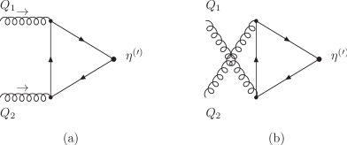
Figure 2: The Feynman diagrams of $g^{*}g^{*}\rightarrow\eta(\eta^{\prime})$ transition.

$g^{*}g^{*}\rightarrow\eta(\eta^{\prime})$ includes two different types of contributions. One is the contribution of diagram of the magnetic penguin operator, and the other is the quark-loop diagram as shown in Fig. 3.

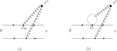
Figure 3: The Feynman diagrams for $B\rightarrow\rho\eta^{(\prime)}$ decays when considering SHSM. The solid dots represent $g^{*}g^{*}\rightarrow\eta(\eta^{\prime})$ transition as shown in Fig. 2.

The amplitude of the magnetic penguin operator is

$$F_{O_{8g}}^{q(s)} =-i\dfrac{2}{N_{c}^{3}}f_{B}f_{\rho}^{||}f_{q(s)}m_{B}^{4}\int_{0}^{1}du\int dx_{1}dx_{2}\int b_{2}db_{2}$$ (68)

$$\times b_{3}db_{3}\int_{0}^{2\pi}d\theta\int d\xi dk_{\perp}k_{\perp}(\dfrac{m_{B}}{2}+\dfrac{|\vec{k_{\perp}}|^{2}}{2\xi^{2}m_{B}})K(\vec{k})$$

$$\times(E_{Q}+m_{Q})J_{0}(k_{\perp}b_{3})\alpha_{s}^{2}(\mu^{\prime})(1-x_{1})\phi_{\eta_{q(s)}}(x_{2},b_{2})$$

$$\times\{(E_{q}-k^{3})\phi_{\rho}(x_{1},b_{3})+r_{\rho}r_{f}[x_{1}E_{q}-(x_{1}-2)k^{3}]$$

$$\times\phi_{\rho}^{s}(x_{1},b_{3})+r_{\rho}r_{f}[(x_{1}-2)E_{q}-x_{1}k^{3}]\phi_{\rho}^{t}(x_{1},b_{3})\}$$

$$\times h^{\prime}(\xi,1-x_{1},1-x_{2},b_{3},b_{2},\theta,u,m_{B})S_{t}(x_{1})$$

$$\times exp[-S_{B}(\mu^{\prime})-S_{\eta_{q(s)}}(\mu^{\prime})-S_{\rho}(\mu^{\prime})|_{{b_{1}}\rightarrow{b_{3}}}].$$

The amplitude of the quark loop is

$$F_{QL}^{q(s)} =i\dfrac{2\pi}{N_{c}^{3}}f_{B}f_{\rho}^{||}f_{q(s)}m_{B}^{2}\int_{0}^{1}du\int dx_{1}dx_{2}\int b_{2}db_{2}$$ (69)

$$\times b_{3}db_{3}\int_{0}^{2\pi}d\theta\int d\xi dk_{\perp}k_{\perp}(\dfrac{m_{B}}{2}+\dfrac{|\vec{k_{\perp}}|^{2}}{2\xi^{2}m_{B}})K(\vec{k})$$

$$\times(E_{Q}+m_{Q})J_{0}(k_{\perp}b_{3})\alpha_{s}^{2}(\mu^{\prime})(1-x_{1})(1-\xi)$$

$$\times\phi_{\eta_{q(s)}}(x_{2},b_{2})\{(E_{q}-k^{3})\phi_{\rho}(x_{1},b_{3})+2r_{\rho}r_{f}k^{3}$$

$$\times\phi_{\rho}^{s}(x_{1},b_{3})-2r_{\rho}r_{f}E_{q}\phi_{\rho}^{t}(x_{1},b_{3})\}$$

$$\times h_{d}(\xi,1-x_{2},1-x_{1},b_{3},b_{2})S_{t}(x_{1})$$

$$\times exp[-S_{B}(\mu^{\prime})-S_{\eta_{q(s)}}(\mu^{\prime})-S_{\rho}(\mu^{\prime})|_{{b_{1}}\rightarrow{b_{3}}}].$$

where

$$h^{\prime}(\xi,1-x_{1},1-x_{2},b_{3},b_{2},\theta,u,m_{B})=\left\{\begin{aligned} \dfrac{\sqrt{b_{2}^{2}+b_{3}^{2}-2b_{2}b_{3}\cos\theta}}{2\sqrt{(1-x_{1})(\xi-u)}m_{B}}&K_{-1}(\sqrt{(1-x_{1})(\xi-u)}m_{B}\sqrt{b_{2}^{2}+b_{3}^{2}-2b_{2}b_{3}\cos\theta})&\\ \times&K_{0}(-i\sqrt{(1-x_{1})(1-x_{2})}m_{B}b_{2}),&\\ &\quad\quad\quad\quad\quad\quad\quad\quad\quad\quad\quad\quad\quad\quad\quad\quad\quad\mathrm{for}\;\xi\geq u,\\ &&\\ i\dfrac{\sqrt{b_{2}^{2}+b_{3}^{2}-2b_{2}b_{3}\cos\theta}}{2\sqrt{(1-x_{1})(u-\xi)}m_{B}}&K_{-1}(-i\sqrt{(1-x_{1})(u-\xi)}m_{B}\sqrt{b_{2}^{2}+b_{3}^{2}-2b_{2}b_{3}\cos\theta})&\\ \times&K_{0}(-i\sqrt{(1-x_{1})(1-x_{2})}m_{B}b_{2}),&\\ &\quad\quad\quad\quad\quad\quad\quad\quad\quad\quad\quad\quad\quad\quad\quad\quad\quad\mathrm{for}\;\xi\leq u,\end{aligned}\right.$$ (70)

$$\mu^{\prime}=\mbox{max}(\sqrt{1-x_{1}}m_{B},\dfrac{1}{b_{3}},\dfrac{1}{b_{2}}).$$ (71)

For the decay channels we considered in this work, the additional contributions from the SHSM to decay amplitudes are

$$\mathcal{M}_{g^{*}g^{*}\rightarrow\eta(\eta^{\prime})}(B^{-}\rightarrow\rho^{-}\eta) = -V_{t}C^{\mathrm{eff}}_{8g}(\mu^{\prime})(\sqrt{2}\cos\phi\cdot F_{O_{8g}}^{q}-\sin\phi\cdot F_{O_{8g}}^{s})$$ (72)

$$+\sum_{q^{\prime}=u,c,t}V_{q^{\prime}}C^{(q^{\prime})}(\mu^{\prime},\langle l^{2}\rangle)(\sqrt{2}\cos\phi\cdot F_{QL}^{q}-\sin\phi\cdot F_{QL}^{s}),$$

$$\mathcal{M}_{g^{*}g^{*}\rightarrow\eta(\eta^{\prime})}(B^{-}\rightarrow\rho^{-}\eta^{\prime}) = -V_{t}C^{\mathrm{eff}}_{8g}(\mu^{\prime})(\sqrt{2}\sin\phi\cdot F_{O_{8g}}^{q}+\cos\phi\cdot F_{O_{8g}}^{s})$$ (73)

$$+\sum_{q^{\prime}=u,c,t}V_{q^{\prime}}C^{(q^{\prime})}(\mu^{\prime},\langle l^{2}\rangle)(\sqrt{2}\sin\phi\cdot F_{QL}^{q}+\cos\phi\cdot F_{QL}^{s}),$$

$$\sqrt{2}\mathcal{M}_{g^{*}g^{*}\rightarrow\eta(\eta^{\prime})}(\bar{B^{0}}\rightarrow\rho^{0}\eta) = V_{t}C^{\mathrm{eff}}_{8g}(\mu^{\prime})(\sqrt{2}\cos\phi\cdot F_{O_{8g}}^{q}-\sin\phi\cdot F_{O_{8g}}^{s})$$ (74)

$$-\sum_{q^{\prime}=u,c,t}V_{q^{\prime}}C^{(q^{\prime})}(\mu^{\prime},\langle l^{2}\rangle)(\sqrt{2}\cos\phi\cdot F_{QL}^{q}-\sin\phi\cdot F_{QL}^{s}),$$

$$\sqrt{2}\mathcal{M}_{g^{*}g^{*}\rightarrow\eta(\eta^{\prime})}(\bar{B^{0}}\rightarrow\rho^{0}\eta^{\prime}) = V_{t}C^{\mathrm{eff}}_{8g}(\mu^{\prime})(\sqrt{2}\sin\phi\cdot F_{O_{8g}}^{q}+\cos\phi\cdot F_{O_{8g}}^{s})$$ (75)

$$-\sum_{q^{\prime}=u,c,t}V_{q^{\prime}}C^{(q^{\prime})}(\mu^{\prime},\langle l^{2}\rangle)(\sqrt{2}\sin\phi\cdot F_{QL}^{q}+\cos\phi\cdot F_{QL}^{s}),$$

where $V_{u}=V_{ub}V_{ud}^{*}$, $V_{c}=V_{cb}V_{cd}^{*}$ and $V_{t}=V_{tb}V_{td}^{*}$.

IV The Contribution of Soft Transition Form Factors

In the numberical calculations, we take the critical infrared cutoff scale as $\mu_{c}=1\;\mathrm{GeV}$, at which the soft and hard contributions in QCD are seaprated LY2021 ; LY2023 ; WY2023 ; LWY2024 . Contributions with energy scale $\mu>\mu_{c}$ can be calculated with perturbative QCD. While, for contributions with the scale $\mu<\mu_{c}$, $B\rho$, $B\eta_{q}$, $B\eta_{s}$ soft transition form factors and $\rho\eta_{q}$, $\rho\eta_{s}$ soft production form factors are introduced to describe these soft contributions. It has been shown in Ref. WY2023 that the physical results only slightly depend on the choice of the value of $\mu_{c}$ around 1 GeV. Therefore, it is resonable to choose the infrared cutoff scale as $\mu_{c}=1\;\mathrm{GeV}$.

We find that among the eight types of Feynman diagrams shown in Fig. 1, the non-perturbative soft contributions from Figs. 1(c)-(f) are very small and can be neglected. For $B\rightarrow\rho\eta^{(\prime)}$ decays, contributions from the soft production form factors in Figs. 1(g) and 1(h) alway cancel between the diagrams interchanging $\rho$ and $\eta^{(\prime)}$ in the final state. Therefore, only the contributions from the soft transition form factors corresponding to Figs. 1(a) and 1(b) remaines.

Due to the quark composition of $\eta_{s}$, we only consider the transition form factors of $B\rightarrow\eta_{q}$ and $B\rightarrow\rho$. The form factors can be divided into two parts

$$\begin{split}&F_{+}^{B\eta_{q}}=h_{+}^{B\eta_{q}}+\xi_{+}^{B\eta_{q}},\\ &A_{0}^{B\rho}=h_{A_{0}}^{B\rho}+\xi_{A_{0}}^{B\rho},\end{split}$$ (76)

where $h_{+}^{B\eta_{q}}$ and $h_{A_{0}}^{B\rho}$ are the hard form factors that are contributed by hard interactions, and $\xi_{+}^{B\eta_{q}}$ and $\xi_{A_{0}}^{B\rho}$ the soft form factors that are dominated by soft dynamics. Thus, the amplitude is modified as

$$\mathcal{M}(B^{-}\rightarrow\rho^{-}\eta) \rightarrow \mathcal{M}(B^{-}\rightarrow\rho^{-}\eta)+\cos\phi\dfrac{1}{\sqrt{2}}$$ (77)

$$\times[2if_{\rho}^{||}V_{\mathrm{CKM}}C_{\eta_{q}\rho}(\mu_{c})\xi_{+}^{B\eta_{q}}$$

$$+2if_{q}V_{\mathrm{CKM}}C_{\rho\eta_{q}}(\mu_{c})\xi_{A_{0}}^{B\rho}$$

$$-\sin\phi[2if_{s}V_{\mathrm{CKM}}C_{\rho\eta_{s}}\xi_{A_{0}}^{B\rho}],$$

where $V_{\mathrm{CKM}}$ and $C_{\rho\eta}(\mu_{c})$ represent the product of CKM matrix elements and the combination of the Wilson coefficients relevant to the operators $(V-A)(V-A)$, $(V-A)(V+A)$ and $(S+P)(S-P)$, respectively. For $\bar{B^{0}}\rightarrow\rho^{0}\eta$ decay, $\cos\phi\dfrac{1}{\sqrt{2}}(\sin\phi)$ should be replaced by $\cos\phi\dfrac{1}{2}(\sin\phi\dfrac{1}{\sqrt{2}})$. When considering decays in $\eta^{\prime}$, only the relevant mixing pattern should be changed.

V The Contribution of Color-Octet quark-antiquark pairs in the long-range within the final state

Since the quark-antiquark pair in mesons should be in color-singlet state, the contributions of quark-antiquark pair in color-octet state in the final state is not considered in $B$ meson decays in general. In principle, as the quark-antiquark pair in color-octet state moves away from each other to the hadronic scale, they can change to color-singlet state by exchanging soft gluons. Therefore, the contributions of color-octet quark-antiquark pairs in the final state of $B$ decays may not be zero. Previously, we have applied the color-octet mechanism to $B\rightarrow PP$ decays LWY2024 . In this work, we will consider the colot-octet contribution in decays of $B\rightarrow\rho\eta^{(\prime)}$.

Utilizing the relation for the generators of the color SU(3) group

$$T^{a}_{ij}T^{a}_{kl}=-\dfrac{1}{2N_{c}}\delta_{ij}\delta_{kl}+\dfrac{1}{2}\delta_{il}\delta_{kj},$$ (78)

we can separate the contributions of color-singlet and color-octet states LWY2024 .

Taking Figs. 1(a) and 1(b) as example, we briefly explain the main steps. Let’s consider the operator insertion of $(\bar{b}_{j}q_{i})(\bar{q}^{\prime}_{i}q^{\prime}_{j})$ in Fig. 4.

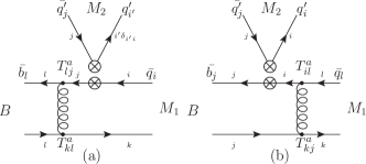
Figure 4: Factorizable diagrams with the insertion of $(\bar{b}_{j}q_{i})(\bar{q}^{\prime}_{i}q^{\prime}_{j})$ operator, where $i,j,k,l$ are color indices, adn the specific type of the current in the operators are ommitted.

The color factors in Fig. 4(a) is

$$\begin{split}\sum_{ijkli^{\prime}}T_{kl}^{a}T_{lj}^{a}\delta_{i^{\prime}i}&=\sum_{ijki^{\prime}}C_{F}\delta_{kj}\delta_{i^{\prime}i}\\ &=\sum_{ijki^{\prime}}C_{F}\left(\dfrac{1}{N_{c}}\delta_{ki}\delta_{i^{\prime}j}+2T_{ki}^{a}T_{i^{\prime}j}^{a}\right),\end{split}$$ (79)

while for Fig. 4(b), the color factor becomes

$$\begin{split}&\sum_{ijkl}T_{il}^{a}T_{kj}^{a}=\sum_{ijkl}\left[-\dfrac{1}{2N_{c}}\delta_{il}\delta_{kj}+\dfrac{1}{2}\delta_{ij}\delta_{kl}\right]\\ &\quad=\sum_{ijkl}\left[-\dfrac{1}{2N_{c}}\left(\dfrac{1}{N_{c}}\delta_{ij}\delta_{kl}+2T_{ij}^{b}T_{kl}^{b}\right)+\dfrac{1}{2}\delta_{ij}\delta_{kl}\right]\\ &\quad=\sum_{ijkl}\left(\dfrac{C_{F}}{N_{c}}\delta_{ij}\delta_{kl}-\dfrac{1}{N_{c}}T_{ij}^{b}T_{kl}^{b}\right),\end{split}$$ (80)

where the first and second terms represent the contributions of color-singlet and color-octet states, respectively. If we consider the insertion of the operator $(\bar{b}_{i}q_{i})(\bar{q}^{\prime}_{j}q^{\prime}_{j})$ in Fig. 4, there are no contributions of the color-octet state. In addition, we need to introduce phenomenological parameters $Y^{8}_{F}$ and $Y^{8}_{M}$ to characterize the magnitude of color-octet contributions for factorizable and nonfactorizable diagrams, respectively. For the Figs. 4(a) and 4(b), the result is

$$Y^{8}_{F}F_{e}^{(R,P)8},$$ (81)

where $F_{e}^{(R,P)8}\equiv 2N_{c}^{2}F_{e}^{(R,P)a}-\dfrac{N_{c}}{C_{F}}F_{e}^{(R,P)b}$. The symbel without the superscript $(R,P)$ represents the result of $(V-A)(V-A)$ current, while the superscript $R$ and $P$ represent the currents of $(V-A)(V+A)$ and $(S+P)(S-P)$ operators, respectively. Here the distribution amplitudes of quark-antiquark pairs in color-octet state are assumed as the same as that of color-singlet state.

In $B\rightarrow\rho\eta^{(\prime)}$ decays, there are no extral color-octet contributions from Figs. 1(g) and 1(h), all the soft contributions can be included into the soft form factros. The contributions of Fis. 1(c), 1(d), 1(e) and 1(f) are

$$Y^{8}_{M}M_{e}^{(R,P)\prime 8},\;Y^{8}_{M}M_{e}^{(R,P)8},\;Y^{8}_{M}M_{a}^{(R,P)8},$$ (82)

where

$$M_{e}^{(R,P)\prime 8}\equiv\dfrac{N_{c}^{2}}{C_{F}}M_{e}^{(R,P)},M_{a}^{(R,P)8}\equiv-\dfrac{N_{c}}{C_{F}}M_{a}^{(R,P)},$$

$$M_{e}^{(R,P)8}\equiv 2N_{c}^{2}M_{e}^{(R,P)c}-\dfrac{N_{c}}{C_{F}}M_{e}^{(R,P)d},$$ (83)

where $F_{e}^{(R,P)a}$, $F_{e}^{(R,P)b}$, $M_{e}^{(R,P)}$, $M_{e}^{(R,P)c}$, $M_{e}^{(R,P)d}$ and $M_{a}^{(R,P)}$ are the hard amplitudes given in Eqs. (21)$-$(37). The decay amplitudes in Eqs. (44)-(47) are modified as

$$\sqrt{2}\mathcal{M}(B^{-}\rightarrow\rho^{-}\eta_{q}) \rightarrow \sqrt{2}\mathcal{M}(B^{-}\rightarrow\rho^{-}\eta_{q})+[V_{u}{C_{2}}-V_{t}(C_{3}+2C_{4}-\dfrac{1}{2}C_{9}+\dfrac{1}{2}C_{10})]Y^{8\rho\eta_{q}}_{F}F^{8}_{e\rho\eta_{q}}$$ (84)

$$-V_{t}(2C_{6}+\dfrac{1}{2}C_{8})Y^{8\rho\eta_{q}}_{F}F_{e\rho\eta_{q}}^{R8}-V_{t}(C_{5}-\dfrac{1}{2}C_{7})Y^{8\rho\eta_{q}}_{F}F_{e\rho\eta_{q}}^{P8}$$

$$+[V_{u}C_{1}-V_{t}(C_{3}+C_{9})]Y^{8\rho\eta_{q}}_{F}F^{8}_{e\eta_{q}\rho}-V_{t}(C_{5}+C_{7})Y^{8\rho\eta_{q}}_{F}F_{e\eta_{q}\rho}^{P8}$$

$$+[V_{u}C_{2}-V_{t}(C_{3}+2C_{4}-\dfrac{1}{2}C_{9}+\dfrac{1}{2}C_{10})]Y^{8\rho\eta_{q}}_{M}M^{8}_{e\rho\eta_{q}}-V_{t}(C_{5}-\dfrac{1}{2}C_{7})Y^{8\rho\eta_{q}}_{M}M_{e\rho\eta_{q}}^{R8}$$

$$+[V_{u}C_{1}-V_{t}(C_{4}+2C_{3}-\dfrac{1}{2}C_{10}+\dfrac{1}{2}C_{9})]Y^{8\rho\eta_{q}}_{M}M^{\prime 8}_{e\rho\eta_{q}}-V_{t}(C_{6}-\dfrac{1}{2}C_{8})Y^{8\rho\eta_{q}}_{M}M_{e\rho\eta_{q}}^{R\prime 8}$$

$$-V_{t}(2C_{6}+\dfrac{1}{2}C_{8})Y^{8\rho\eta_{q}}_{M}M_{e\rho\eta_{q}}^{P8}-V_{t}(2C_{5}+\dfrac{1}{2}C_{7})Y^{8\rho\eta_{q}}_{M}M_{e\rho\eta_{q}}^{P\prime 8}$$

$$+[V_{u}C_{1}-V_{t}(C_{3}+C_{9})]Y^{8\rho\eta_{q}}_{M}M^{8}_{e\eta_{q}\rho}+[V_{u}C_{2}-V_{t}(C_{4}+C_{10})]Y^{8\rho\eta_{q}}_{M}M^{\prime 8}_{e\eta_{q}\rho}$$

$$-V_{t}(C_{5}+C_{7})Y^{8\rho\eta_{q}}_{M}M_{e\eta_{q}\rho}^{R8}-V_{t}(C_{6}+C_{8})Y^{8\rho\eta_{q}}_{M}M_{e\eta_{q}\rho}^{R\prime 8}$$

$$+[V_{u}C_{1}-V_{t}(C_{3}+C_{9})]Y^{8\rho\eta_{q}}_{M}(M^{8}_{a\rho\eta_{q}}+M^{8}_{a\eta_{q}\rho})-V_{t}(C_{5}+C_{7})Y^{8\rho\eta_{q}}_{M}(M_{a\rho\eta_{q}}^{R8}+M_{a\eta_{q}\rho}^{R8}),$$

$$\mathcal{M}(B^{-}\rightarrow\rho^{-}\eta_{s}) \rightarrow \mathcal{M}(B^{-}\rightarrow\rho^{-}\eta_{q})-V_{t}(C_{4}-\dfrac{1}{2}C_{10})Y^{8\rho\eta_{s}}_{F}F^{8}_{e\rho\eta_{s}}-V_{t}(C_{6}-\dfrac{1}{2}C_{8})Y^{8\rho\eta_{s}}_{F}F_{e\rho\eta_{s}}^{R8}$$ (85)

$$-V_{t}(C_{4}-\dfrac{1}{2}C_{10})Y^{8\rho\eta_{s}}_{M}M^{8}_{e\rho\eta_{s}}-V_{t}(C_{3}-\dfrac{1}{2}C_{9})Y^{8\rho\eta_{s}}_{M}M^{\prime 8}_{e\rho\eta_{s}}$$

$$-V_{t}(C_{6}-\dfrac{1}{2}C_{8})Y^{8\rho\eta_{s}}_{M}M_{e\rho\eta_{s}}^{P8}-V_{t}(C_{5}-\dfrac{1}{2}C_{7})Y^{8\rho\eta_{s}}_{M}M_{e\rho\eta_{s}}^{P\prime 8},$$

$$2\mathcal{M}(\bar{B^{0}}\rightarrow\rho^{0}\eta_{q}) \rightarrow 2\mathcal{M}(\bar{B^{0}}\rightarrow\rho^{0}\eta_{q})-[V_{u}{C_{2}}-V_{t}(C_{3}+2C_{4}-\dfrac{1}{2}C_{9}+\dfrac{1}{2}C_{10})]Y^{8\rho\eta_{q}}_{F}F^{8}_{e\rho\eta_{q}}$$ (86)

$$+V_{t}(2C_{6}+\dfrac{1}{2}C_{8})Y^{8\rho\eta_{q}}_{F}F_{e\rho\eta_{q}}^{R8}+V_{t}(C_{5}-\dfrac{1}{2}C_{7})Y^{8\rho\eta_{q}}_{F}F_{e\rho\eta_{q}}^{P8}-V_{t}\dfrac{3}{2}C_{8}Y^{8\rho\eta_{q}}_{F}F_{e\eta_{q}\rho}^{R8}$$

$$+[V_{u}C_{2}-V_{t}(-C_{3}+\dfrac{1}{2}C_{9}+\dfrac{3}{2}C_{10})]Y^{8\rho\eta_{q}}_{F}F^{8}_{e\eta_{q}\rho}+V_{t}(C_{5}-\dfrac{1}{2}C_{7})Y^{8\rho\eta_{q}}_{F}F_{e\eta_{q}\rho}^{P8}$$

$$-[V_{u}C_{2}-V_{t}(C_{3}+2C_{4}-\dfrac{1}{2}C_{9}+\dfrac{1}{2}C_{10})]Y^{8\rho\eta_{q}}_{M}M^{8}_{e\rho\eta_{q}}+V_{t}(C_{5}-\dfrac{1}{2}C_{7})Y^{8\rho\eta_{q}}_{M}M_{e\rho\eta_{q}}^{R8}$$

$$-[V_{u}C_{1}-V_{t}(C_{4}+2C_{3}-\dfrac{1}{2}C_{10}+\dfrac{1}{2}C_{9})]Y^{8\rho\eta_{q}}_{M}M^{\prime 8}_{e\rho\eta_{q}}+V_{t}(C_{6}-\dfrac{1}{2}C_{8})Y^{8\rho\eta_{q}}_{M}M_{e\rho\eta_{q}}^{R\prime 8}$$

$$+V_{t}(2C_{6}+\dfrac{1}{2}C_{8})Y^{8\rho\eta_{q}}_{M}M_{e\rho\eta_{q}}^{P8}+V_{t}(2C_{5}+\dfrac{1}{2}C_{7})Y^{8\rho\eta_{q}}_{M}M_{e\rho\eta_{q}}^{P\prime 8}$$

$$+[V_{u}C_{2}-V_{t}(-C_{3}+\dfrac{1}{2}C_{9}+\dfrac{3}{2}C_{10})]Y^{8\rho\eta_{q}}_{M}M^{8}_{e\eta_{q}\rho}+V_{t}(C_{5}-\dfrac{1}{2}C_{7})Y^{8\rho\eta_{q}}_{M}M_{e\eta_{q}\rho}^{R8}$$

$$+[V_{u}C_{1}-V_{t}(-C_{4}+\dfrac{1}{2}C_{10}+\dfrac{3}{2}C_{9})]Y^{8\rho\eta_{q}}_{M}M^{\prime 8}_{e\eta_{q}\rho}+V_{t}(C_{6}-\dfrac{1}{2}C_{8})Y^{8\rho\eta_{q}}_{M}M_{e\eta_{q}\rho}^{R\prime 8}$$

$$-V_{t}\dfrac{3}{2}C_{8}Y^{8\rho\eta_{q}}_{M}M_{e\eta_{q}\rho}^{P8}-V_{t}\dfrac{3}{2}C_{7}Y^{8\rho\eta_{q}}_{M}M_{e\eta_{q}\rho}^{P\prime 8}$$

$$+[V_{u}C_{2}-V_{t}(-C_{3}+\dfrac{1}{2}C_{9}+\dfrac{3}{2}C_{10})]Y^{8\rho\eta_{q}}_{M}(M^{8}_{a\rho\eta_{q}}+M^{8}_{a\eta_{q}\rho})$$

$$+V_{t}(C_{5}-\dfrac{1}{2}C_{7})Y^{8\rho\eta_{q}}_{M}(M_{a\rho\eta_{q}}^{R8}+M_{a\eta_{q}\rho}^{R8})-V_{t}\dfrac{3}{2}C_{8}Y^{8\rho\eta_{q}}_{M}(M_{a\rho\eta_{q}}^{P8}+M_{a\eta_{q}\rho}^{P8}),$$

$$\sqrt{2}\mathcal{M}(\bar{B^{0}}\rightarrow\rho^{0}\eta_{s}) \rightarrow \sqrt{2}\mathcal{M}(\bar{B^{0}}\rightarrow\rho^{0}\eta_{s})+V_{t}(C_{4}-\dfrac{1}{2}C_{10})Y^{8\rho\eta_{s}}_{F}F^{8}_{e\rho\eta_{s}}+V_{t}(C_{6}-\dfrac{1}{2}C_{8})Y^{8\rho\eta_{s}}_{F}F_{e\rho\eta_{s}}^{R8}$$ (87)

$$+V_{t}(C_{4}-\dfrac{1}{2}C_{10})Y^{8\rho\eta_{s}}_{M}M^{8}_{e\rho\eta_{s}}+V_{t}(C_{3}-\dfrac{1}{2}C_{9})Y^{8\rho\eta_{s}}_{M}M^{\prime 8}_{e\rho\eta_{s}}$$

$$+V_{t}(C_{6}-\dfrac{1}{2}C_{8})Y^{8\rho\eta_{s}}_{M}M_{e\rho\eta_{s}}^{P8}+V_{t}(C_{5}-\dfrac{1}{2}C_{7})Y^{8\rho\eta_{s}}_{M}M_{e\rho\eta_{s}}^{P\prime 8}.$$

VI Numerical Result and Discussion

In the numerical calculations, besides the parameters in the meson wave functions, the other non-perturbative parameters are the soft transition form factors $\xi_{+}^{B\eta_{q}}$, $\xi_{A_{0}}^{B\rho}$ and the color-octet parameters $Y^{8\rho\eta_{q}}_{F}$, $Y^{8\rho\eta_{s}}_{F}$, $Y^{8\rho\eta_{q}}_{M}$ and $Y^{8\rho\eta_{s}}_{M}$.

At the energy scale $\mu>\mu_{c}$, the hard transition form factors can be calculated by using PQCD approach, we have

$$h_{+}^{B\eta_{q}}=0.17\pm 0.01,$$

$$h_{A_{0}}^{B\rho}\ =0.18\pm 0.01.$$ (88)

From the experimental data of semileptonic decays of $B$ meson, as well as the calculation results from nonperturbative method, such as light-cone sum rules (LCSR), etc., the complete transition form factors can be extracted PDG2024 ; PB-RZ2005 ; AK-TM-NO2007 ; AB-DMS-RZ2021 ; NG-AK-DVD2020 ; JG-CDL-YLS-YMW-YBW2020 ; MAI-JGK-SGK-CDR2007 ; MAI-JGK-SGK-PS-GGS2012

$$F_{+}^{B\eta_{q}}=0.23\pm 0.03,$$

$$A_{0}^{B\rho}\ =0.32\pm 0.05.$$ (89)

The value of $F_{+}^{B\eta_{q}}$ is obtained by using the experimental data on the branching ratios of semileptonic decays of $B$ meson PDG2024 . The numerical value of $A_{0}^{B\rho}$ is derived as the average of calculated results from LCSR, SCET and Quark Model PB-RZ2005 ; AK-TM-NO2007 ; AB-DMS-RZ2021 ; NG-AK-DVD2020 ; JG-CDL-YLS-YMW-YBW2020 ; MAI-JGK-SGK-CDR2007 ; MAI-JGK-SGK-PS-GGS2012 . Based on the above results, we can obtain the values of soft transition form factors

$$\xi_{+}^{B\eta_{q}}=0.06\pm 0.02,$$

$$\xi_{A_{0}}^{B\rho}\ =0.14\pm 0.04.$$ (90)

For the color-octet parameters, since perturbative method cannot be applied for calculating them, their values are determined by fitting the experimental data of $B\rightarrow\rho\eta^{(\prime)}$ decays. We find that there are two different parameter solutions that can all yield the best results, and we denote them as $a$ and $b$. The obtained results are given in Table I.

Table 1: The values of color-octet parameters.

	$Y^{8\rho\eta_{q}}_{F}$	$Y^{8\rho\eta_{s}}_{F}$	$Y^{8\rho\eta_{q}}_{M}$	$Y^{8\rho\eta_{s}}_{M}$
$a$	$(0.171^{+0.039}_{-0.078})e^{i\pi(1.394^{+0.106}_{-0.058})}$	$(0.172^{+0.038}_{-0.075})e^{i\pi(1.625^{+0.159}_{-0.284})}$	$(0.187^{+0.020}_{-0.038})e^{i\pi(1.159^{+0.054}_{-0.043})}$	$(0.196^{+0.013}_{-0.031})e^{i\pi(0.860^{+0.114}_{-0.057})}$
$b$	$(0.163^{+0.009}_{-0.008})e^{i\pi(0.174^{+0.032}_{-0.028})}$	$(0.017^{+0.019}_{-0.014})e^{i\pi(0.289^{+0.146}_{-0.204})}$	$(0.165^{+0.008}_{-0.004})e^{i\pi(0.203^{+0.029}_{-0.030})}$	$(0.205^{+0.002}_{-0.002})e^{i\pi(0.286^{+0.021}_{-0.019})}$

The comparison of the theoretical results and experimental data for the branching ratios and direct $CP$ violations of $B\rightarrow\rho\eta^{(\prime)}$ decays are presented in Table II.

Column “$\mathrm{LO_{NLOWC}}$” in Table II represents the leading-order contribution of QCD with NLO Wilson coefficients. Column “NLO” represents the contribution up to next-to-leading-order in QCD including the vertex corrections, quark loops and magnetic penguin contributions. In Column “NLO+$g^{*}g^{*}$”, the contribution of SHSM is included. In Column “NLO+$g^{*}g^{*}+\xi^{B\rho}+\xi^{B\eta_{q}}$”, the contributions of NLO, SHSM of $g^{*}g^{*}$ fusion and soft transition form factors are included. “soft” denotes the contributions of soft transition form factors and color-octet parameters.

The first uncertainty in the theoretical result comes from the uncertainties of soft transition form factors and color-octet parameters. The second and third uncertainties originate from the uncertainties of the parameters in $B$ and light meson wave functions, respectively.

Table 2: $B\rightarrow\rho\eta^{(\prime)}$ branching ratios and $CP$ violations.

	$\mathrm{LO_{NLOWC}}$	NLO	NLO+$g^{*}g^{*}$	$\begin{aligned} &\text{NLO}+g^{*}g^{*}\\ &+\xi^{B\rho}+\xi^{B\eta_{q}}\end{aligned}$	NLO+$g^{*}g^{*}$+softa	NLO+$g^{*}g^{*}$+softb	Data PDG2024
Br($B^{0}\rightarrow\rho^{0}\eta$)$\times 10^{-6}$	0.002	0.01	0.01	0.05	$0.15\pm 0.09^{+0.00+0.00}_{-0.00-0.00}$	$0.28\pm 0.04^{+0.00+0.00}_{-0.00-0.00}$	$<$1.5
Br($B^{+}\rightarrow\rho^{+}\eta$)$\times 10^{-6}$	3.45	3.66	3.68	6.49	$9.35\pm 2.02^{+0.14+0.29}_{-0.23-0.29}$	$9.42\pm 1.51^{+0.14+0.29}_{-0.23-0.29}$	7.0$\pm$2.9
Br($B^{0}\rightarrow\rho^{0}\eta^{\prime}$)$\times 10^{-6}$	0.01	0.01	0.02	0.07	$1.21\pm 0.20^{+0.00+0.00}_{-0.00-0.00}$	$1.26\pm 0.08^{+0.00+0.00}_{-0.00-0.00}$	$<$1.3
Br($B^{+}\rightarrow\rho^{+}\eta^{\prime}$)$\times 10^{-6}$	2.08	1.84	1.94	2.58	$7.83\pm 1.38^{+0.07+0.14}_{-0.11-0.14}$	$7.69\pm 1.07^{+0.07+0.14}_{-0.11-0.14}$	9.7$\pm$2.2
$A_{CP}$($B^{0}\rightarrow\rho^{0}\eta$)	0.94	0.84	0.82	0.22	$-0.72\pm 0.35^{+0.01+0.07}_{-0.01-0.09}$	$-0.51\pm 0.30^{+0.01+0.07}_{-0.01-0.09}$	-
$A_{CP}$($B^{+}\rightarrow\rho^{+}\eta$)	0.00	$-$0.08	$-$0.09	$-$0.14	$0.14\pm 0.08^{+0.00+0.00}_{-0.00-0.00}$	$0.15\pm 0.07^{+0.00+0.00}_{-0.00-0.00}$	0.11$\pm$0.11
$A_{CP}$($B^{0}\rightarrow\rho^{0}\eta^{\prime}$)	0.69	0.67	0.62	0.04	$-0.29\pm 0.33^{+0.02+0.08}_{-0.03-0.09}$	$-0.35\pm 0.33^{+0.02+0.08}_{-0.03-0.09}$	-
$A_{CP}$($B^{+}\rightarrow\rho^{+}\eta^{\prime}$)	0.10	0.20	0.16	0.34	$0.14\pm 0.11^{+0.00+0.03}_{-0.00-0.03}$	$0.17\pm 0.11^{+0.00+0.03}_{-0.00-0.03}$	0.26$\pm$0.17

Comparing the results in the first and seond coloumns in Table 2, one can see that the NLO contributions only slightly affect the decay amplitudes. The branching ratios are only changed by less than 10% for most decay modes. Only for $B^{0}\rightarrow\rho^{0}\eta$ decay, the effect of NLO contribution is dramatically large. This is because the leading order contribution is doubly suppressed by the color and isospin structures of the tree-level diagrams for this decy mode. The SHSM effect from $g^{*}g^{*}$ fusion process is also very small. Only the soft transition form factors and especially the color-octet contributions can enhance the branching ratios effectively, which is important for explaining the experimental data. For the experimental measured decay modes, the calculated branching ratios and $CP$ violations can be in good agreement with eperimental data. We also predict the branching raios and $CP$ violations for $B^{0}\rightarrow\rho^{0}\eta$ and $\rho^{0}\eta^{\prime}$ decays, which have not been well measured yet in experiment. These predictions can be tested in experiment in the future.

VII Summary

We study $B\rightarrow\rho\eta$, $\rho\eta^{\prime}$ decays in the modified perturbative QCD approach, where a critical infrared cutoff scale $\mu_{c}$ is introduced. For contributions at scales larger than $\mu_{c}$, PQCD approach can be applied. For contributions at scale $\mu<\mu_{c}$, soft transition form factors are introduced to describe these contributions. In addition, color-octet contribution is introduced, where the quark-antiquark pairs in $B$ decay can be in color-octet state after short-distance interactions, then color-octet quark-antiquark pairs can be changed to color-singlet state by exchanging soft gluons at long-distance of hadronic scale. By selecting reasonable input parameters, we find the experimental data can be well explained by the modified PQCD approach. We also predict branching ratios and $CP$ violations for two decay modes which have not been well detected in experiment. These predictions can be testet in experiment in future.

Appendix A Threshold and Sudakov factor

Threshold factor $S_{t}(x)$ can be found in Ref. lihn2002 as

$$S_{t}(x)=\frac{2^{1+2c}\Gamma(3/2+c)}{\sqrt{\pi}\Gamma(1+c)}[x(1-x)]^{c},$$ (91)

where $c=0.3$.

The exponentials $\exp[-S_{B,\eta_{q(s)},\rho}(\mu)]$ include the Sudakov factors associated with the mesons and the relevant single ultraviolet logarithms. The exponent parts are

$$S_{B}(\mu)=s(x,b,m_{B})-\frac{1}{\beta_{1}}\ln\frac{\ln(\mu/\Lambda_{\mbox{QCD}})}{\ln(1/(b\Lambda_{\mbox{QCD}}))},$$ (92)

$$S_{\eta_{q(s)},\rho}(\mu) = s(x,b,m_{B})+s(1-x,b,m_{B})$$ (93)

$$\;\;-\frac{1}{\beta_{1}}\ln\frac{\ln(\mu/\Lambda_{\mbox{QCD}})}{\ln(1/(b\Lambda_{\mbox{QCD}}))},$$

where $s(x,b,Q)$ up to next-to-leading order is Li1995

$$s(x,b,Q)=\frac{A^{(1)}}{2\beta_{1}}\hat{q}\ln\left(\frac{\hat{q}}{\hat{b}}\right)-\frac{A^{(1)}}{2\beta_{1}}\left(\hat{q}-\hat{b}\right)+\frac{A^{(2)}}{4\beta_{1}^{2}}\left(\frac{\hat{q}}{\hat{b}}-1\right)-\left[\frac{A^{(2)}}{4\beta_{1}^{2}}-\frac{A^{(1)}}{4\beta_{1}}\ln\left(\frac{e^{2\gamma_{E}-1}}{2}\right)\right]\ln\left(\frac{\hat{q}}{\hat{b}}\right)$$

$$+\frac{A^{(1)}\beta_{2}}{4\beta_{1}^{3}}\hat{q}\left[\frac{\ln(2\hat{q})+1}{\hat{q}}-\frac{\ln(2\hat{b})+1}{\hat{b}}\right]+\frac{A^{(1)}\beta_{2}}{8\beta_{1}^{3}}\left[\ln^{2}(2\hat{q})-\ln^{2}(2\hat{b})\right]$$

$$+\frac{A^{(1)}\beta_{2}}{8\beta_{1}^{3}}\ln\left(\frac{e^{2\gamma_{E}-1}}{2}\right)\left[\frac{\ln(2\hat{q})+1}{\hat{q}}-\frac{\ln(2\hat{b})+1}{\hat{b}}\right]-\frac{A^{(1)}\beta_{2}}{16\beta_{1}^{4}}\left[\frac{2\ln(2\hat{q})+3}{\hat{q}}-\frac{2\ln(2\hat{b})+3}{\hat{b}}\right]$$

$$-\frac{A^{(1)}\beta_{2}}{16\beta_{1}^{4}}\frac{\hat{q}-\hat{b}}{\hat{b}^{2}}\left[2\ln(2\hat{b})+1\right]+\frac{A^{(2)}\beta_{2}^{2}}{432\beta_{1}^{6}}\frac{\hat{q}-\hat{b}}{\hat{b}^{3}}\left[9\ln^{2}(2\hat{b})+6\ln(2\hat{b})+2\right]$$

$$+\frac{A^{(2)}\beta_{2}^{2}}{1728\beta_{1}^{6}}\left[\frac{18\ln^{2}(2\hat{q})+30\ln(2\hat{q})+19}{\hat{q}^{2}}-\frac{18\ln^{2}(2\hat{b})+30\ln(2\hat{b})+19}{\hat{b}^{2}}\right],$$ (94)

with $\hat{q}$ and $\hat{b}$ being defined as

$${\hat{q}}\equiv{\rm ln}\left(xQ/(\sqrt{2}\Lambda_{QCD})\right),~{}{\hat{b}}\equiv{\rm ln}(1/b\Lambda_{QCD}).$$ (95)

The coefficients $\beta_{i}$ and $A^{(i)}$ are

$$\beta_{1}=\frac{33-2n_{f}}{12}\;,\;\;\;\beta_{2}=\frac{153-19n_{f}}{24}\;,A^{(1)}=\frac{4}{3}\;,$$

$$A^{(2)}=\frac{67}{9}-\frac{\pi^{2}}{3}-\frac{10}{27}n_{f}+\frac{8}{3}\beta_{1}\ln\left(\frac{e^{\gamma_{E}}}{2}\right)\;,$$ (96)

where $\gamma_{E}$ is the Euler constant.

Appendix B Light Meson Distribution Amplitudes

The light-cone distribution amplitudes of the light mesons are $\phi_{\eta_{q(s)}}(x,k_{\perp})$, $\phi^{\eta_{q(s)}}_{P}(x,k_{\perp})$, $\phi^{\eta_{q(s)}}_{\sigma}(x,k_{\perp})$, $\phi_{\rho}(x,k_{\perp})$, $\phi_{\rho}^{t}(x,k_{\perp})$ and $\phi_{\rho}^{s}(x,k_{\perp})$. Assuming the dependence of transverse momentum takes the form of Gaussian distribution, when transforming the function to b-space, we have wy2002

$$\phi(x,b)=\phi(x)\exp\left(-\frac{b^{2}}{4\beta^{2}}\right).$$ (97)

For the distribution amplitudes of $\eta_{q(s)}$ and $\rho$ mesons we use $\beta=4.0\;\mathrm{GeV}^{-1}$ wy2002 ; JK93 . For $\eta_{q(s)}$ meson, the twist-2 and twist-3 distribution amplitudes are given by Ball-Braun2006

$$\phi_{\eta_{q(s)}}(x)=6x(1-x)\biggl{[}1+a_{1}^{\eta_{q(s)}}C_{1}^{3/2}(t)+a_{2}^{\eta_{q(s)}}C_{2}^{3/2}(t)\biggr{]},$$ (98)

$$\phi_{P}^{\eta_{q(s)}}(x)=1+a_{0P}^{\eta_{q(s)}}+a_{1P}^{\eta_{q(s)}}C_{1}^{1/2}(t)+a_{2P}^{\eta_{q(s)}}C_{2}^{1/2}(t)+a_{3P}^{\eta_{q(s)}}C_{3}^{1/2}(t)+a_{4P}^{\eta_{q(s)}}C_{4}^{1/2}(t)+b_{1P}^{\eta_{q(s)}}\ln(x)+b_{2P}^{\eta_{q(s)}}\ln(1-x),$$ (99)

$$\begin{split}\phi_{\sigma}^{\eta_{q(s)}}(x)&=6x(1-x)\biggl{[}1+a_{0\sigma}^{\eta_{q(s)}}+a_{1\sigma}^{\eta_{q(s)}}C_{1}^{3/2}(t)+a_{2\sigma}^{\eta_{q(s)}}C_{2}^{3/2}(t)+a_{3\sigma}^{\eta_{q(s)}}C_{3}^{3/2}(t)\biggr{]}\\ &\quad+9x(1-x)\biggl{[}b_{1\sigma}^{\eta_{q(s)}}\ln(x)+b_{2\sigma}^{\eta_{q(s)}}\ln(1-x)\biggr{]},\\ \end{split}$$ (100)

where $t=2x-1$ and $C$ functions are Gegenbauer polynomials. The coefficients in distribution amplitudes are as follows,

$$\begin{split}&a_{1}^{\eta_{q}}=0,\quad a_{2}^{\eta_{q}}=0.25\pm 0.15,\\ &a_{0P}^{\eta_{q}}=0.079\pm 0.028,\quad a_{2P}^{\eta_{q}}=0.95\pm 0.33,\\ &a_{4P}^{\eta_{q}}=0.14\pm 0.11,\quad a_{1P}^{\eta_{q}}=a_{3P}^{\eta_{q}}=0,\\ &b_{1P}^{\eta_{q}}=b_{2P}^{\eta_{q}}=0.039\pm 0.014,\\ &a_{0\sigma}^{\eta_{q}}=0.055\pm 0.024,\quad a_{2\sigma}^{\eta_{q}}=0.18\pm 0.07,\\ &a_{1\sigma}^{\eta_{q}}=a_{3\sigma}^{\eta_{q}}=0,\quad b_{1\sigma}^{\eta_{q}}=b_{2\sigma}^{\eta_{q}}=0.026\pm 0.009,\\ \end{split}$$ (101)

for the $\eta_{q}$ meson, and

$$\begin{split}&a_{1}^{\eta_{s}}=0,\quad a_{2}^{\eta_{s}}=0.25\pm 0.15,\\ &a_{0P}^{\eta_{s}}=1.13\pm 0.41,\quad a_{2P}^{\eta_{s}}=0.99\pm 0.48,\\ &a_{4P}^{\eta_{s}}=0.06\pm 0.05,\quad a_{1P}^{\eta_{s}}=a_{3P}^{\eta_{s}}=0,\\ &b_{1P}^{\eta_{s}}=b_{2P}^{\eta_{s}}=0.56\pm 0.20,\\ &a_{0\sigma}^{\eta_{s}}=0.79\pm 0.34,\quad a_{2\sigma}^{\eta_{s}}=0.14\pm 0.07,\\ &a_{1\sigma}^{\eta_{s}}=a_{3\sigma}^{\eta_{s}}=0,\quad b_{1\sigma}^{\eta_{s}}=b_{2\sigma}^{\eta_{s}}=0.38\pm 0.14,\\ \end{split}$$ (102)

for the $\eta_{s}$ meson.

For $\rho$ meson, the twist-2 and twist-3 distribution amplitudes are given by PB-GWJ2007

$$\phi_{\rho}(x)=6x(1-x)[1+a_{1}^{||}C_{1}^{3/2}(t)+a_{2}^{||}C_{2}^{3/2}(t)],$$ (103)

$$\begin{split}\phi_{\rho}^{t}(x)=&3t^{2}+\dfrac{3}{2}a_{1}^{\perp}t(3t^{2}-1)+\dfrac{3}{2}a_{2}^{\perp}t^{2}(5t^{2}-3)+(\dfrac{15}{2}\kappa_{3}^{\perp}-\dfrac{3}{4}\lambda_{3}^{\perp})t(5t^{2}-3)+\dfrac{5}{8}\omega_{3}^{\perp}(35t^{4}-30t^{2}+3)\\ &+\dfrac{3}{2}\dfrac{m_{q}+m_{q}}{m_{\rho}}\dfrac{f_{\rho}^{||}}{f_{\rho}^{\perp}}\biggl{\{}1+8a_{1}^{||}t+3a_{2}^{||}[7-30x(1-x)]+t(1+3a_{1}^{||}+6a_{2}^{||})\ln(1-x)\\ &-t(1-3a_{1}^{||}+6a_{2}^{||})\ln x\biggr{\}},\\ \end{split}$$ (104)

$$\begin{split}\Psi_{3}^{||}(x)=&6x(1-x)\biggl{[}1+(\dfrac{1}{3}a_{1}^{\perp}+\dfrac{5}{3}\kappa_{3}^{\perp})C_{1}^{3/2}(t)+(\dfrac{1}{6}a_{2}^{\perp}+\dfrac{5}{18}\omega_{3}^{\perp})C_{2}^{3/2}(t)-\dfrac{1}{20}\lambda_{3}^{\perp}C_{3}^{3/2}(t)\biggr{]}\\ &+3\dfrac{m_{q}+m_{q}}{m_{\rho}}\dfrac{f_{\rho}^{||}}{f_{\rho}^{\perp}}\biggl{\{}x(1-x)[1+2a_{1}^{||}t+3a_{2}^{||}(7-5x(1-x))]+(1+3a_{1}^{||}+6a_{2}^{||})(1-x)\ln(1-x)\\ &+(1-3a_{1}^{||}+6a_{2}^{||})x\ln x\biggr{\}},\\ \end{split}$$ (105)

where $t=2x-1$, $C$ functions are Gegenbauer polynomials and $\phi_{\rho}^{s}(x)=\dfrac{1}{2}\dfrac{d\Psi_{3}^{||}(x)}{dx}$. The coefficients in distribution amplitudes are as follows,

$$\begin{split}&a_{1}^{||}=0,\quad a_{2}^{||}=0.15\pm 0.07,\\ &a_{1}^{\perp}=0,\quad a_{2}^{\perp}=0.14\pm 0.06,\\ &\kappa_{3}^{\perp}=0,\quad\omega_{3}^{\perp}=0.55\pm 0.25,\\ &\lambda_{3}^{\perp}=0,\quad m_{q}=0.0056\pm 0.0016\end{split}$$ (106)

The above parameters are determined at the renormalization scale of $\mu=1.0~{}\mathrm{GeV}$. The Gegenbauer polynomials are given by

$$C_{1}^{1/2}(t)=t,\quad C_{2}^{1/2}(t)=\frac{1}{2}\left(3t^{2}-1\right),\quad C_{3}^{1/2}(t)=\frac{1}{2}t\left(5t^{2}-3\right),\quad C_{4}^{1/2}(t)=\frac{1}{8}\left(35t^{4}-30t^{2}+3\right),\quad$$ (107)

and

$$C_{1}^{3/2}(t)=3t,\quad C_{2}^{3/2}(t)=\frac{3}{2}\left(5t^{2}-1\right),\quad C_{3}^{3/2}(t)=\frac{5}{2}t\left(7t^{2}-3\right),\quad C_{4}^{3/2}(t)=\frac{15}{8}\left(21t^{4}-14t^{2}+1\right).\quad$$ (108)

References

- (1) Y. Y. Keum, H. N. Li, and A. I. Sanda, Phys. Lett. B 504, 6 (2001).
- (2) Y. Y. Keum, H. N. Li, and A. I. Sanda, Phys. Rev. D 63, 054008 (2001).
- (3) C. D. Lü, K. Ukai, and M. Z. Yang, Phys. Rev. D 63, 074009 (2001).
- (4) M. Beneke, G. Buchalla, M. Neubert, and C.T. Sachrajda, Phys. Rev. Lett. 83, 1914 (1999).
- (5) M. Beneke, G. Buchalla, M. Neubert, and C.T. Sachrajda, Nucl. Phys. B591, 313 (2000).
- (6) M. Beneke, G. Buchalla, M. Neubert, and C.T. Sachrajda, Nucl. Phys. B606, 245 (2001).
- (7) M. Beneke and M. Neubert, Nucl. Phys. B675, 333 (2003).
- (8) S. Navas et al. (Particle Data Group), Phys. Rev. D 110, 030001 (2024).
- (9) A.J. Buras, R. Fleischer, S. Recksiegel, and F. Schwab, Eur. Phys. J. C 32, 45 (2003).
- (10) H.N. Li, S. Mishima, and A.I. Sanda, Phys. Rev. D 72, 114005 (2005).
- (11) H.N. Li and S. Mishima, Phys. Rev. D 83, 034023 (2011).
- (12) H.N. Li and S. Mishima, Phys. Rev. D 90, 074018 (2014).
- (13) Y.L. Zhang, Y.Y. Liu, Y.Y. Fan, S. Cheng, and Z. J. Xiao, Phys. Rev. D 90, 014029 (2014).
- (14) W. Bai, M. Liu, Y. Y. Fan, W. F. Wang, S. Cheng, and Z. J. Xiao, Chin. Phys. C 38, 033101 (2014).
- (15) M. Beneke and D. Yang, Nucl. Phys. B 736, 34 (2006).
- (16) M.Beneke and S. Jager, Nucl. Phys. B 751, 160 (2006).
- (17) G. Bell, Nucl. Phys. B 795, 1 (2008).
- (18) V. Pilipp, Nucl. Phys. B 794,154 (2008).
- (19) M. Beneke, T. Huber, and X. Q. Li, Nucl. Phys. B 832, 109 (2010).
- (20) J. Chai, S. Cheng, Y. H. Ju, D. C. Yan, C. D. L, and Z. J. Xiao, Chin. Phys. C 46, 123103 (2022).
- (21) H. Y. Cheng and C. K. Chua, Phys. Rev. D 80, 074031 (2009).
- (22) H. Y. Cheng and C. K. Chua, Phys. Rev. D 80, 114008 (2009).
- (23) Q. Chang, J. Sun, Y. Yang, and X. Li, Phys. Rev. D 90, 054019 (2014).
- (24) X. Liu, H. N. Li, and Z. J. Xiao, Phys. Rev. D 93, 014024 (2016).
- (25) S. Lü and M. Z. Yang, Nucl. Phys. B 972, 115550 (2021).
- (26) S. Lü and M. Z. Yang, Phys. Rev. D 107, 013004 (2023).
- (27) R. X. Wang and M. Z. Yang, Phys. Rev. D 108, 013003 (2023).
- (28) S. Lü, R. X. Wang and M. Z. Yang, Phys. Rev. D 110, 056025 (2024).
- (29) G. Buchalla, A.J. Buras, M.E. Lautenbacher, Rev. Mod. Phys. 68, 1125 (1996).
- (30) M.Z. Yang, Eur. Phys. J. C 72, 1880 (2012).
- (31) J.B. Liu and M.Z. Yang, J. High Energy Phys. 07 (2014) 106.
- (32) J.B. Liu and M.Z. Yang, Phys. Rev. D 91, 094004 (2015).
- (33) H.K. Sun and M.Z. Yang, Phys. Rev. D 95, 113001 (2017).
- (34) H. K. Sun and M. Z. Yang, Phys. Rev. D 99, 093002 (2019).
- (35) V.M. Braun, I.E. Filyanov, Z. Phys. C 48, 239 (1990).
- (36) P. Ball, J. High Energy Phys. 01 (1999) 010.
- (37) M. Beneke, T. Feldmann, Nucl. Phys. B 592, 3 (2001).
- (38) Z.T. Wei, M.Z. Yang, Nucl. Phys. B 642, 263 (2002).
- (39) T. Kurimoto, H.n. Li and A.I. Sanda, Phys.Rev.D 65, 014007 (2002)
- (40) P. Ball, V.M. Braun, Y. Koike, K. Tanaka, Nucl. Phys. B 529, 323 (1998).
- (41) Th. Feldmann, P. Kroll, B. Stech, Phys. Rev. D 58, 114006 (1998).
- (42) Th. Feldmann, P. Kroll, B. Stech, Phys. Lett. B 449, 339 (1999).
- (43) P. Ball, V.M. Braun, and A. Lenz, J. High Energy Phys. 05 (2006) 004.
- (44) H.N. Li and H.L. Yu, Phys. Rev. D 53, 2480 (1996).
- (45) H.N. Li and H.L. Yu, Phys. Rev. D 53, 4970 (1996).
- (46) H.N. Li, Phys. Rev. D 66, 094010 (2002).
- (47) H.N. Li and S. Mishima Phys. Rev. D 74, 094020(2006).
- (48) D.S. Du, C.S. Kim, Y.D. Yang, Phys. Lett. B 426, 133 (1998).
- (49) M.R. Ahmady, E. Kou, A. Sugamoto, Phys. Rev. D 58, 014015 (1998).
- (50) D.S. Du and M.Z. Yang,Phys. Rev. D 57, 5332 (1998).
- (51) T. Muta and M.Z. Yang,Phys. Rev. D 61, 054007 (2000).
- (52) M.Z. Yang and Y.D. Yang,Nucl. Phys. B 609, 469 (2001).
- (53) P. Ball and R. Zwicky, Phys. Rev. D 71, 014029 (2005).
- (54) A. Khodjamirian, T. Mannel, and N. Offen, Phys. Rev. D 75, 054013 (2007).
- (55) A. Bharucha, D. M. Straub, and R. Zwicky, J. High Energy Phys. 08 (2021) 098.
- (56) N. Gubernari, A. Kokulu, and D. van Dyk, J. High Energy Phys. 01 (2020) 150.
- (57) J. Gao, C.D. Lü, Y.L. Shen, Y.M. Wang, and Y.B.Wei, Phys. Rev. D 101, 074035 (2020).
- (58) M.A. Ivanov, J.G. Korner, S.G. Kovalenko, and C. D. Roberts, Phys. Rev. D 76, 034018 (2007).
- (59) M.A. Ivanov, J.G. Korner, S.G. Kovalenko, P. Santorelli, and G.G. Saidullaeva, Phys. Rev. D 85, 034004 (2012).
- (60) H.N. Li, Phys. Rev. D 52, 3958 (1995).
- (61) R. Kakob, P. Kroll, Phys. Lett. B 315, 463 (1993).
- (62) P. Ball and G.W. Jones, J. High Energy Phys. 03 (2007) 069.