Mixtures of In-Context Learners

Abstract

In-context learning (ICL) adapts LLMs by providing demonstrations without fine-tuning the model parameters; however, it does not differentiate between demonstrations and quadratically increases the complexity of Transformer LLMs, exhausting the memory. As a solution, we propose Mixtures of In-Context Learners (MoICL), a novel approach to treat subsets of demonstrations as experts and learn a weighting function to merge their output distributions based on a training set. In our experiments, we show performance improvements on 5 out of 7 classification datasets compared to a set of strong baselines (up to +13% compared to ICL and LENS). Moreover, we enhance the Pareto frontier of ICL by reducing the inference time needed to achieve the same performance with fewer demonstrations. Finally, MoICL is more robust to out-of-domain (up to +11%), imbalanced (up to +49%), or noisy demonstrations (up to +38%) or can filter these out from datasets. Overall, MoICL is a more expressive approach to learning from demonstrations without exhausting the context window or memory.

Mixtures of In-Context Learners

Giwon Hong¹ Emile van Krieken¹ Edoardo M. Ponti¹ Nikolay Malkin¹ Pasquale Minervini^{1,2 1}University of Edinburgh, United Kingdom   ²Miniml.AI, United Kingdom {giwon.hong, p.minervini}@ed.ac.uk

1 Introduction

In-context learning (ICL), where we condition a large language model (LLM) on a set of input–output examples (demonstrations) to perform a wide range of tasks (Brown et al., 2020; Wei et al., 2022), is a transformative technique in NLP. However, in ICL, the context length of the model severely limits the maximum number of in-context demonstrations (Wei et al., 2022), and its effectiveness can vary significantly depending on what demonstrations are selected (Lu et al., 2022; Chen et al., 2023). Current methods for selecting demonstrations are largely heuristic and do not adequately quantify the influence of individual examples on the generalisation properties of the model (Lu et al., 2024).

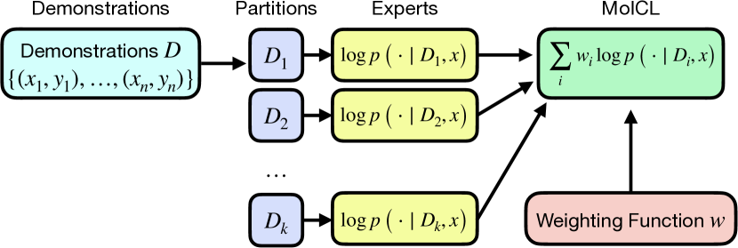
Figure 1: A Mixture of In-Context Learners (MoICL) first partitions a set of demonstrations $D$ in $k$ partitions to create $k$ experts trained via in-context learning, and then combines their next-token predictions via a trainable weighting function.

In general settings, demonstrations are often selected randomly over different seeds or based on simple criteria (Xu et al., 2024), which can lead to suboptimal performance. But is each demonstration high quality and useful, or merely noise? And can we automate this distinction? We propose Mixtures of In-Context Learners (MoICL), a method for dynamically learning how different sets of examples contribute to the prediction task. MoICL prompts an LLM with multiple subsets of examples, and combines their next-token distributions via a weighting function that can be trained via gradient-based optimisation methods; Fig. 1 shows a high-level outline of the method.

We analyse the generalisation properties of MoICL in the following settings: (1) presence of out-of-distribution (OOD) demonstrations, where some in-context demonstrations are sourced from a different dataset; and (2) label imbalance, where the training label distribution is significantly skewed towards a subset of labels. (3) noised demonstrations, where the labels of some demonstrations are perturbed to be completely incorrect. In all three cases, we find that MoICL produces significantly more accurate results than ICL.

Furthermore, MoICL does not require access to the internal parameters of the LLM, making it applicable to black-box LLMs, and it significantly reduces the complexity issues arising from the quadratic time and memory complexity in sequence length of self-attention since it allows the distribution of the training samples among multiple experts. We also show that the method can be made more efficient by sparsifying the mixing weights.

We summarise our contributions as follows:

• We introduce the Mixture of In-Context Learners (MoICL), which assigns weights to each demonstration subset and learns from them, dynamically identifying the optimal experts and anti-experts via gradient-based optimisation.

• We demonstrate that MoICL is competitive with standard ICL while being significantly more data, memory, and computationally efficient.

• We show that MoICL is resilient to noisy demonstrations and label imbalance.

2 Mixtures of In-Context Learners

2.1 In-context Learning

Given a large language model (LLM) with next-token distribution $p(\cdot)$, a set of $n$ demonstrations $D$ = {$(x_{1},y_{1})...(x_{n},y_{n})$} and an input text $x$, the model generates a response $y$ when prompted with the concatenation of the examples in $D$ and the input text $x$:

$$y \sim p(y\mid x_{1},y_{1},\dots,x_{n},y_{n},x)$$ (1)

$$=p(y\mid D,x),$$

we refer to the model in Eq. 1 as concat-based ICL (Min et al., 2022a). With concat-based ICL, given a demonstration set $D$, the model can generate a response $y$ for the input text $x$ without needing task-specific fine-tuning or access to the model parameters. However, concat-based ICL is still problematic: recent works show that it is very sensitive to the choice of the prompts and in-context demonstrations (Voronov et al., 2024); the number of demonstrations is bounded by the maximum context size (Brown et al., 2020); and, in Transformer-based LLMs, the cost of self-attention operations grows quadratically with the number of in-context samples (Liu et al., 2022).

2.2 Mixtures of In-Context Learners

We propose Mixtures of In-Context Learners (MoICL), a method for addressing the limitations of concat-based ICL (Section 2.1). We first partition (Section B.1) the set of demonstrations $D$ into $k$ disjoint subsets $D_{1},\ldots,D_{k}$:

$$D=D_{1}\sqcup D_{2}\sqcup\ldots\sqcup D_{k}.$$ (2)

Then, each demonstration subset $D_{i}\subseteq D$ is passed to the LLM along with the input text $x$, and we denote these as experts. The next-token distributions of the experts are combined using a vector of mixing weights $w\in\mathbb{R}^{k}$:

$$p\left(y\mid D,x\right)\propto\exp\left[\sum_{i=1}^{k}w_{i}\log p\left(y\mid D_{i},x\right)\right]$$ (3)

where each $w_{i}\in\mathbb{R}$ represents the contribution of the expert denoted by $p\left(y\mid D_{i},x\right)$ to the final next-token distribution $p\left(y\mid D,x\right)$, and each expert $p\left(y\mid D_{i},x\right)$ is trained via concat-based ICL, as in Eq. 1. 

Weighting Functions.

We consider the following weighting functions for calculating the weight $w_{i}\in\mathbb{R}$ of the $i$-th expert in MoICL:

Scalar weights.

Use a vector of trainable parameters $w\in\mathbb{R}^{k}$, where $w_{i}$ denotes the weight associated to the $i$-th expert. The weights $w$ are initialised as $\forall i:w_{i}=1/k$.

Hyper-network.

Use a hyper-network (Ha et al., 2017) $h_{\phi}(\cdot)$ with parameters $\phi$ to generate the weights of each expert $w_{i}$, given all in-context demonstration subsets concatenated: $w_{1},\ldots,w_{k}=h_{\phi}(D_{1},\ldots,D_{k})$.

We learn the parameters of the weighting function $w$ by maximising the conditional log-likelihood of a training set $D_{T}$. One advantage of using a hyper-network $h_{\phi}$ for dynamically computing the weights $w$ over having $w$ as a set of parameters is that the model can provide weights for sets of demonstrations not seen during training.

Sparsifying the Mixture Weights

One limitation of MoICL is that, for each token, it requires invoking the base LLM $k$ times, one for each expert with a different set of in-context examples. To solve this issue, we propose to sparsify the weighting coefficients $w\in\mathbb{R}^{k}$ so that only $k^{\prime}<k$ of them have non-zero values. To achieve this, we define the output of the weighting function as:

$$w=w^{\prime}\odot\text{top-}k^{\prime}(m),$$ (4)

where $w^{\prime}\in\mathbb{R}^{k}$ are scalar weights for the $k$ experts, $m\in\mathbb{R}^{k}$ is a set of masking coefficients, $\text{top-}k^{\prime}:\mathbb{R}^{k}\mapsto\{0,1\}^{k}$ is a function that produces a mask that selects the highest $k^{\prime}$ elements of a $k$-dimensional input vector, and $\odot$ is the element-wise product. To back-propagate through the rationale extraction process, we use Implicit Maximum Likelihood Estimation (IMLE; Niepert et al., 2021; Minervini et al., 2023), a gradient estimation method for back-propagating through continuous-discrete functions like $\text{top-}k^{\prime}$ into neural architectures. More specifically, let $\widehat{m}=\text{top-}k^{\prime}(m)\in\{0,1\}^{k}$ denote the $\text{top-}k^{\prime}$ mask. In our experiments using IMLE, we estimate the gradient of the loss w.r.t. the masking coefficients $\nabla_{m}\mathcal{L}$ as $\nabla_{m}\mathcal{L}\approx\text{top-}k^{\prime}(m)-\text{top-}k^{\prime}(m+\lambda\nabla_{\widehat{m}}\mathcal{L})$, where $\lambda\in\mathbb{R}_{+}$ is a hyperparameter selected by the user.

Method $\downarrow$ Dataset $\rightarrow$ Offensive Hate SST2 RTE FEVER PAWS QNLI Concat-based ICL 76.44$\pm$2.48 53.54$\pm$4.29 95.46$\pm$0.14 86.43$\pm$1.26 80.63$\pm$0.49 78.12$\pm$0.77 89.08$\pm$0.44 Random Search 77.88$\pm$1.14 58.09$\pm$1.93 95.76$\pm$0.18 86.57$\pm$1.43 82.13$\pm$0.10 78.88$\pm$0.57 89.99$\pm$0.26 Ensemble-based ICL (Min et al., 2022a) 73.35$\pm$0.44 53.68$\pm$4.27 95.48$\pm$0.12 86.43$\pm$1.34 80.63$\pm$0.46 65.27$\pm$0.48 88.57$\pm$0.21 LENS Li and Qiu (2023) 78.70$\pm$0.67 53.20$\pm$3.11 93.81$\pm$0.16 84.98$\pm$0.74 80.07$\pm$0.29 75.60$\pm$0.72 89.04$\pm$0.40 PEFT (LoRA, Hu et al., 2022) 79.79$\pm$4.07 53.76$\pm$4.98 85.89$\pm$6.32 88.88$\pm$2.78 59.78$\pm$0.62 54.82$\pm$3.08 57.24$\pm$4.77 Mixture of ICL (uniform)    $k=5$ 73.77$\pm$1.60 59.29$\pm$1.23 95.39$\pm$0.30 83.10$\pm$1.28 80.12$\pm$0.64 75.37$\pm$0.53 89.65$\pm$0.22    $k=10$ 74.00$\pm$0.87 61.70$\pm$1.61 94.91$\pm$0.19 79.93$\pm$0.81 77.47$\pm$0.89 73.49$\pm$0.46 89.65$\pm$0.14    $k=30$ 73.37$\pm$0.34 59.12$\pm$0.47 94.17$\pm$0.21 77.26$\pm$1.02 79.46$\pm$0.36 65.29$\pm$0.51 88.66$\pm$0.25 Mixture of ICL (scalar)    $k=5$ 78.35$\pm$1.49 66.03$\pm$3.31 95.46$\pm$0.35 84.12$\pm$1.07 81.43$\pm$0.90 77.56$\pm$0.53 89.99$\pm$0.44    $k=10$ 79.42$\pm$1.48 66.52$\pm$2.62 95.32$\pm$0.27 83.32$\pm$1.60 82.04$\pm$0.98 79.42$\pm$0.79 90.44$\pm$0.27    $k=30$ 81.33$\pm$0.69 63.45$\pm$1.69 94.79$\pm$0.34 79.93$\pm$0.93 82.66$\pm$0.38 79.50$\pm$0.33 90.11$\pm$0.20

Table 1: Comparison between baseline methods and the proposed Mixture of In-Context Learners across classification tasks using Llama-3-8B-Instruct. $k$ represents the number of demonstrations subset, where the total number of demonstrations is 30. Bold text signifies the highest accuracy for each task.

3 Experimental Setup

Models

For our experiments, we primarily used Llama-3-8B and its instruction-tuned models, Llama-3-8B-Instruct (AI@Meta, 2024) as our base LLMs. We use Llama-3-8B-Instruct for classification tasks, and Llama-3-8B was used for an open-ended generation task; we use greedy decoding for generating from MoICL. Furthermore, we use Llama-2-7b-chat, 13b-chat, and 70b-chat (Touvron et al., 2023) for analysing the influence of model scale in  Section 4.9. For the hyper-network, in our experiments, we used the T5 models (efficient-tiny, efficient-mini, t5-small, t5-base) (Raffel et al., 2020).

Datasets

To study how well MoICL performs on classification tasks, we use the TweetEval (Barbieri et al., 2020) offensive/hate, SST2 (Socher et al., 2013), RTE (Bentivogli et al., 2009), FEVER (Thorne et al., 2018), PAWS (Zhang et al., 2019), and QNLI (Wang et al., 2018) datasets. For SST2, RTE, FEVER, and QNLI, we report the performance on the development set. For a generation task, we use Natural Questions (NQ; Kwiatkowski et al., 2019) with an open-book setting (Lee et al., 2019).

Baselines

We compare MoICL with the following baselines. Concat-based ICL refers to the standard ICL introduced in  Section 2.1 where all demonstrations are concatenated into a single sequence and passed as input to the LLM along with the input text. Random Search samples random subsets from the demonstration pool, concatenates them, and utilizes them in the same manner as Concat-based ICL. Specifically, we sample $k$ random subsets and select the one that performs best on the training set. Here, $k$ is the maximum number of subsets used in MoICL, and the size of each subset is a random number between 1 and the number of demonstrations $n$. After finding the best subset, we evaluate it on the test set. Ensemble-based ICL (Min et al., 2022a) and LENS (Li and Qiu, 2023) were adjusted in terms of tasks and models to fit our experimental setup. We also report the results of fine-tuning the target model using a parameter-efficient fine-tuning method, namely LoRA (Hu et al., 2022); this is a strong baseline that requires access to the model weights. Finally, we study MoICL Uniform, an ablation that simply weights all experts equally, i.e. $\forall i:w_{i}=1/k$.

Evaluation Metrics

For classification tasks, we use accuracy as the evaluation metric. For generation tasks, we use EM (Exact Match) for NQ-open.

More detailed settings, including dataset statistics, hyperparameters, and implementation details, are provided in Appendix A. Furthermore, in Section B.1, we show that our method is not significantly affected by the choice of partitioning methods. Therefore, we applied static partitioning in all experiments.

4 Results

In our experiments, we aim to answer the following research questions: (1) Does MoICL demonstrate general performance improvements over concat-based ICL and other baselines? (Section 4.1 and  Section 4.2) (2) Is MoICL resilient to problem settings involving label imbalance and noise? (Section 4.4,  Section 4.5 and Section 4.6) (3) Can we select demonstrations (experts) based on the tuned weights? (Section 4.7) (4) Can MoICL handle demonstrations that were not seen during fine-tuning? (Section 4.8) (5) Is MoICL more efficient in terms of data, time, and memory compared to traditional concat-based ICL? (Section 5)

4.1 MoICL in Classification Tasks

To determine the effectiveness of MoICL across various datasets, we compare it with baseline methods in  Table 1. In this experiment, we set the total number of demonstrations ($n$) as 30, and the number of subsets ($k$) as 5, 10, and 30. MoICL outperformed the Baseline ICL on the Offensive, Hate, FEVER, PAWS, and QNLI datasets. The exceptions are SST2 and RTE, where MoICL performs similarly to concat-based ICL in SST2 and shows lower performance in RTE. Surprisingly, MoICL scalar achieved the highest performance with $k$=10 (e.g. in Hate MoICL achieves 66.52, which is about 10 points increase compared to the concat-based ICl) or $k$=30 (e.g. in Offensive MoICL achieves 81.33), rather than $k$=5, in all tasks except for SST2 and RTE. Considering that a larger $k$ reduces the context length (which will be further discussed in Section 5), MoICL manages to capture both efficiency and effectiveness.

4.2 Impact of Partitioning Size

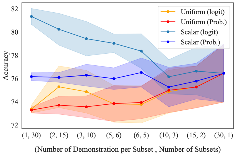
Figure 2: Accuracy according to the number of demonstrations per subset on TweetEval offensive dataset. The shaded area represents the standard deviation. We also compare mixing logits to mixing probabilities; see Section B.2.

In  Fig. 2, we present the performance changes on the test set of TweetEval offensive when varying the number of subsets, $k$. Since the total number of demonstrations is fixed at 30, each subset contains $30/k$ demonstrations, which corresponds to the x-axis of the Figure. Note that when the number of demonstrations per subset is 30 ($k=1$), it corresponds to the standard Concat-based ICL. We observe that Uniform Weights and scalar exhibit distinctly different patterns. With Uniform Weights, as the number of demonstrations per subset decreases, performance tends to decline, which is an expected outcome for ICL. However, with scalar, performance surprisingly increases. This seems to be because the decrease in the number of demonstrations per subset is outweighed by the increased flexibility afforded by having more subsets, each assigned tuned weights by scalar.

4.3 Impact of Non-Negative Weights

MoICL Method ($n,k$=30)	Offensive
uniform	76.44$\pm$2.48
scalar	81.33$\pm$0.69
- Positive Weights Only	76.05$\pm$0.55

Table 2: How important is it to be able to detect anti-experts? Results on the TweetEval Offensive Test set using Llama-3-8B-Instruct. “Positive Weights Only” limits the weights of subsets to positive values, preventing subsets from acting as anti-experts. The number of subsets $k$ and the total number of demonstrations $n$ is 30.

Inspired by Liu et al. (2024), we made an assumption that each expert could also serve as an anti-expert, by allowing the expert weights to be negative. If the weight becomes negative during the training process, this indicates that the expert is not only unhelpful, but is actively being used as an anti-expert in generating the response. To verify this, in  Table 2, we compare the performance when we restrict the weights to be positive. We observe that restricting the weights to be positive, thereby eliminating the possibility for anti-experts, significantly degrades performance. This is because certain demonstrations or their subsets can be useful when utilised as anti-experts. This also greatly aids in interpreting the usefulness of experts, as seen in the experiments from  Section 4.4 and  Section 4.6.

Method ($n,k=30$)	$\mathbf{p}$=0.0	$\mathbf{p}$=0.5	$\mathbf{p}$=0.7
Concat-based ICL	76.44$\pm$2.48	70.67$\pm$5.06	68.49$\pm$4.34
Mixture of ICL
- uniform	73.37$\pm$0.34	72.07$\pm$0.38	70.79$\pm$0.56
- scalar	81.33$\pm$0.69	80.95$\pm$0.65	80.19$\pm$0.37

Table 3: Analysis of out-of-domain (OOD) demonstrations on TweetEval offensive test set using Llama-3-8B-Instruct. Here, $p$ represents the proportion of OOD demonstrations sampled from the SST2 dataset. The number of subsets $k$ and the total number of demonstrations $n$ was set to 30. Bold text signifies the highest accuracy for each $p$.

4.4 Handling Out-of-domain Demonstrations

By learning to associate a weight to each expert, MoICL can be used to identify whether demonstrations are relevant to the task. To analyse this, in Table 3, we present the accuracy of MoICL on the TweetEval offensive test set, using a mix of demonstrations sampled from the SST dataset and those from the TweetEval offensive dataset. We observe that as $p$ (the proportion of OOD demonstrations) increases, the performance of standard ICL methods decreases. However, MoICL (with scalar) effectively mitigates this by reducing the influence of these OOD demonstrations, resulting in the smallest performance drop. This becomes even more apparent when analysing the weights of actual OOD demonstrations. When $p=0.5$ (i.e. the number of OOD and in-domain demonstrations is equal), the average weight of in-domain demonstrations is 0.0108$\pm$0.0025, while the average weight for OOD demonstrations is -0.0059$\pm$0.0027. For $p=0.7$, the average weight of in-domain demonstrations is 0.0127$\pm$0.0052, while the average weight for OOD demonstrations is -0.0019$\pm$0.0016.

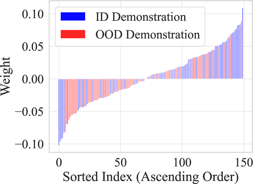
(a) 50% OOD

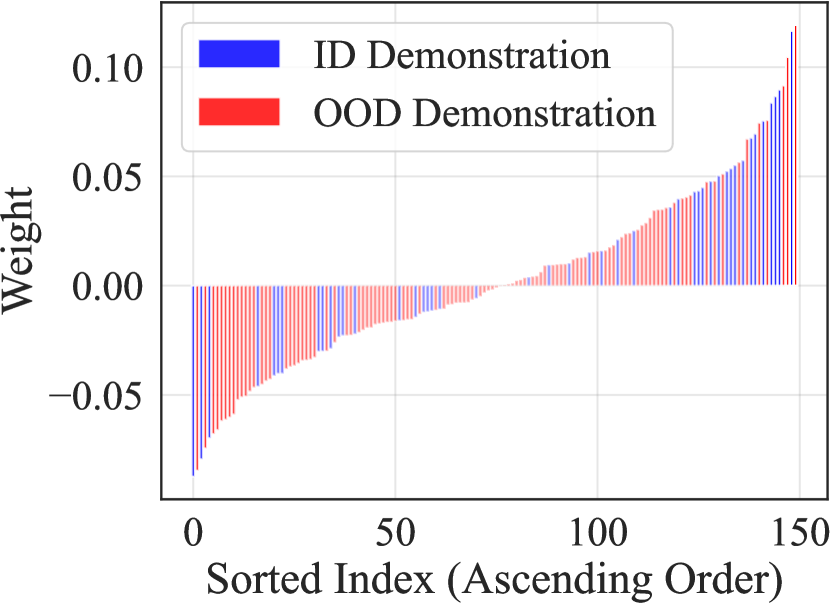
(b) 70% OOD

Figure 3: Visualisation of the tuned weights when (a) 50% and (b) 70% of demonstrations are OOD. The y-axis indicates the weights, whereas the x-axis represents the index of demonstrations sorted in ascending order (across five different seeds). Blue bars correspond to in-domain (ID) demonstrations, and red bars correspond to out-of-domain (OOD) demonstrations.

In  Fig. 3, we visualise how the weights of in-domain demonstrations (blue bars) and OOD demonstrations (red bars) are distributed. We observed a general trend where in-domain demonstrations typically receive positive weights, while OOD demonstrations tend to receive negative weights. This provides evidence that our proposed method successfully mitigates the OOD demonstrations.

4.5 Mitigating Label Imbalance

Method ($n,k=30$)	Original	Imbalanced
Concat-based ICL	76.44$\pm$2.48	28.49$\pm$0.86
Mixture of ICL
- uniform	73.37$\pm$0.34	40.19$\pm$2.32
- scalar	81.33$\pm$0.69	77.77$\pm$1.20

Table 4: Analysis of imbalanced demonstrations on the TweetEval Offensive Test set using Llama-3-8B-Instruct. “Imbalanced” refers to a condition where only one out of 30 demonstrations has a “neutral” label, while the rest are “offensive”.

To determine whether our proposed method can handle label imbalance, on the TweetEval Offensive dataset, we set up 29 “offensive” label demonstrations and one ‘non-offensive’ label demonstration out of 30 demonstrations. Since the TweetEval Offensive dataset has a “non-offensive” to “offensive” label ratio of about 7:3, such imbalanced demonstrations would be detrimental to performance. As seen in  Table 4, such imbalanced demonstrations caused a significant performance drop in standard ICL methods. However, our proposed method (scalar) showed the least performance drop, successfully mitigating the effects of label imbalance.

4.6 Filtering Noisy Demonstrations

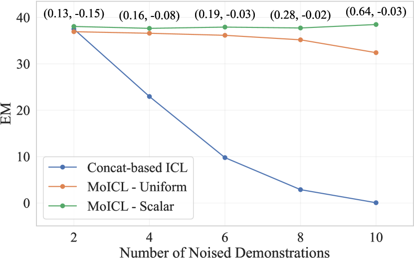
Figure 4: Resilience of ICL to adding noisy demonstration. We report the EM based on the number of noised demonstrations out of the total 12 demonstrations in NQ. For the case of scalar, we also present the average weights of standard and noisy demonstrations as (standard, noisy).

Method $\downarrow$ Subset $\rightarrow$	$k^{\prime}=5$	$k^{\prime}=10$	$k^{\prime}=20$	$k^{\prime}=30$	$k^{\prime}=90$
Concat-based ICL ($n=k^{\prime}$)	72.19$\pm$2.63	74.12$\pm$2.24	74.84$\pm$1.88	76.44$\pm$2.48	75.67$\pm$2.33
MoICL ($n,k=k^{\prime}$)
uniform	73.05$\pm$0.52	73.42$\pm$0.76	73.42$\pm$0.49	73.37$\pm$0.34	73.26$\pm$0.16
scalar	76.26$\pm$1.11	78.16$\pm$0.91	80.16$\pm$1.23	81.33$\pm$0.69	83.35$\pm$0.41
w/ scalar ($n,k=90$)
Highest $k^{\prime}$ Weights	75.58$\pm$0.81	75.56$\pm$0.46	74.42$\pm$0.61	74.33$\pm$0.38	-
Highest $k^{\prime}$ Weights (abs)	69.79$\pm$14.84	60.53$\pm$21.84	71.58$\pm$14.67	72.93$\pm$13.14	-
IMLE Top-$k^{\prime}$ mask	76.07$\pm$0.64	75.93$\pm$0.69	76.35$\pm$0.35	76.44$\pm$0.64	-

Table 5: Analysis of selecting useful demonstrations with the proposed MoICL on the TweetEval Offensive test set on Llama-3-8b-Instruct. ‘Highest $k^{\prime}$ Weights’ refers to selecting the $k^{\prime}$ subsets with the largest weights out of 90 weights of MoICL scalar, while ‘Highest $k^{\prime}$ Weights (abs)’ uses absolute weights instead.

One of the benefits of assigning weights to each demonstration or its subsets is the ability to handle low-quality, or more specifically, noisy demonstrations. To verify this, in NQ-Open, we created noisy demonstrations (see Section B.3 for the result of NQ-open without noised demonstrations) by randomly changing the answers to one of (yes, no, foo, bar), where the total number of demonstration is 12, and each subset has one demonstration ($n$, $k=12$). The results in  Fig. 4 show that our proposed method effectively handles noisy demonstrations. While the performance of the concat-based ICL significantly decreases as the number of noisy demonstrations increases, the MoICL methods can maintain performance. Additionally, without tuning the weights (Uniform Weights), performance gradually declines as the number of noisy demonstrations increases, but with tuning (scalar), the performance remains stable (more than +35% with 10 noised demonstrations). This is clearly evident when analysing the learned weights. In the figure, the average weights of normal and noisy demonstrations are displayed in the form (normal weights, noise weights) for scalar, showing a noticeable difference.

4.7 Selecting Demonstration Subsets

We now analyse the impact of sparsifying the mixture weights $w\in\mathbb{R}^{k}$ in MoICL. Results are available in Table 5 — “Highest $n$ Weights” refers to selecting the subsets with the $n$ largest $w$ weights (or $|w|$ in the case of “abs”), while IMLE Top-$k^{\prime}$ mask refers to the method introduced in Section 2.2, using $\lambda=1$ following the default hyper-parameters proposed by Niepert et al. (2021). While MoICL scalar achieved the highest accuracy, the need to learn them for each $m$ and $k$ makes selection methods that tune weights for a large $n$ and then select $m$ of them more practical. Notably, “Highest $n$ Weights (abs)” is high-variance, indicating the difficulty in effectively leveraging anti-experts (Section 4.3). In contrast, IMLE, which uses a mask, demonstrated stable performance, achieving the best results, particularly with a few demonstrations (when $k^{\prime}=5$).

4.8 Generalization to Unseen Demonstrations

Method $\downarrow$ Dataset $\rightarrow$	Offensive	Hate
Concat-based ICL ($n=30$)	76.44$\pm$2.48	53.54$\pm$4.29
Mixture of ICL ($n,k$=30)
- uniform	73.37$\pm$0.34	59.12$\pm$0.47
- Hyper-network	76.65$\pm$1.31	65.07$\pm$5.22

Table 6: Comparison of MoICL methods, including scalar and Hyper-network, on the TweetEval Offensive and Hate, using Llama-3-8b-Instruct.

While Mixture of ICL with scalar is simpler and less costly, it has the disadvantage of requiring a fixed set of demonstration subsets. This is an inherent limitation of the method itself, which assigns weights to each subset and learns from them. A solution to overcome this limitation is to utilise a smaller, fine-tuned hyper-network (Hyper-network) that calculates the weights for arbitrary demonstration subsets.  Table 6 compares the performance of MoICL methods, where the demonstration set $D$ was not available during the training process. In this situation, scalar, which assumes that the experts and their corresponding demonstrations are fixed, cannot be tuned. However, the Hyper-network fine-tuned on the available demonstrations, can generalize well when presented with unseen demonstration $D$.

4.9 Impact of Model Size

Method $\downarrow$ Model $\rightarrow$	ll2-chat-7b	ll2-chat-13b	ll2-chat-70b
Concat-based ICL	73.09$\pm$3.21	63.09$\pm$3.85	69.42$\pm$1.78
MoICL
- uniform	79.35$\pm$0.22	63.60$\pm$1.84	67.88$\pm$1.03
- scalar	79.16$\pm$0.60	80.49$\pm$1.01	82.26$\pm$0.65

Table 7: Comparison on the TweetEval Offensive Test set across different sizes of the Llama-2 models.

Considering the ongoing trend of scaling up LLMs, it is essential to analyse how the proposed method is affected by model size. In  Table 7, we compare the accuracy of our proposed method on the TweetEval Offensive task when using Llama-2-chat models in various sizes (7B, 13B, 70B) as the target LLM. Although the performance of the Llama-2-7B-chat model is somewhat unusual compared to the other two models, we observed that MoICL consistently outperforms concat-based ICL across all three model sizes.

Hyper-network Model	Offensive	Hate
t5-efficient-tiny (16M)	69.32$\pm$2.07 | 74.60$\pm$2.03	67.32$\pm$0.66 | 60.48$\pm$4.56
t5-efficient-mini (31M)	68.50$\pm$2.01 | 73.74$\pm$1.43	66.00$\pm$1.51 | 56.61$\pm$0.90
t5-small (60M)	71.01$\pm$1.09 | 76.65$\pm$1.31	70.20$\pm$1.53 | 65.07$\pm$5.22
t5-base (220M)	69.14$\pm$1.01 | 74.40$\pm$2.39	68.24$\pm$0.75 | 63.23$\pm$4.51

Table 8: Comparison on the TweetEval Offensive/hate Dev|Test set using Llama-3-8b-Instruct as a target LLM across different sizes of the hyper-network. The numbers in parentheses indicate the number of parameters.

We also analysed the impact of hyper-network model size.  Table 8 compares the dev/test set accuracy on the TweetEval hate/offensive task based on the size of the T5 model used as the hyper-network. From analysing the dev set results, we found that even with a very small model size (16M–60M), the hyper-network performed relatively well, leading us to decide on using T5-small as our hyper-network.

5 Data and Compute Efficiency

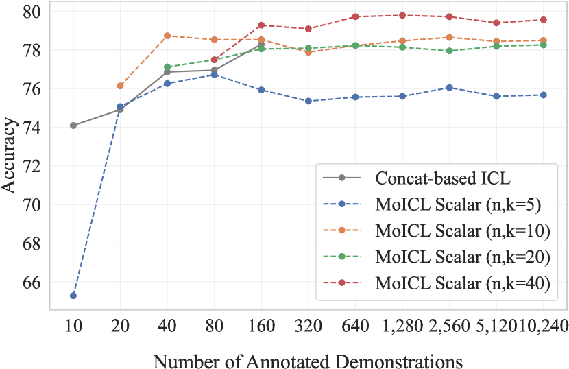
(a) TweetEval Offensive

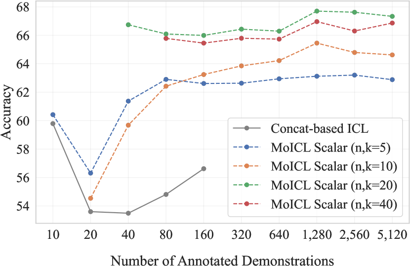
(b) TweetEval Hate

Figure 5: An analysis of MoICL’s data efficiency on the TweetEval offensive/hate test set using Llama-3-8B-Instruct. Concat-based ICL concatenated all available demonstrations (x-axis), though more than 160 exceeded the context length. MoICL Scalar Weights ($k=n$) assigned the designated demonstrations to the experts while using the remaining available demonstrations for fine-tuning.

One potential limitation of MoICL is that it requires training instances for weight tuning, which can be problematic when such training data is unavailable. To analyse the data efficiency of MoICL, we present the accuracy on TweetEval Offensive and Hate test set in  Fig. 5 under scenarios where the number of training instances (Number of Annotated Demonstrations) is limited. In this experiment, we set $n=k$, so each expert is assigned one demonstration and weight tuning is performed using the number of training instances minus $k$ (e.g., when the x-axis is at 40, MoICL with $k=10$ is tuned with 30 training instances). We observed that MoICL is highly data-efficient, achieving better performance than concat-based ICL with only around 20 annotated demonstrations. In contrast, concat-based ICL showed lower performance when given the same number of annotated demonstrations and particularly struggled when the number of demonstrations exceeded 160, as this surpassed the context length limit.

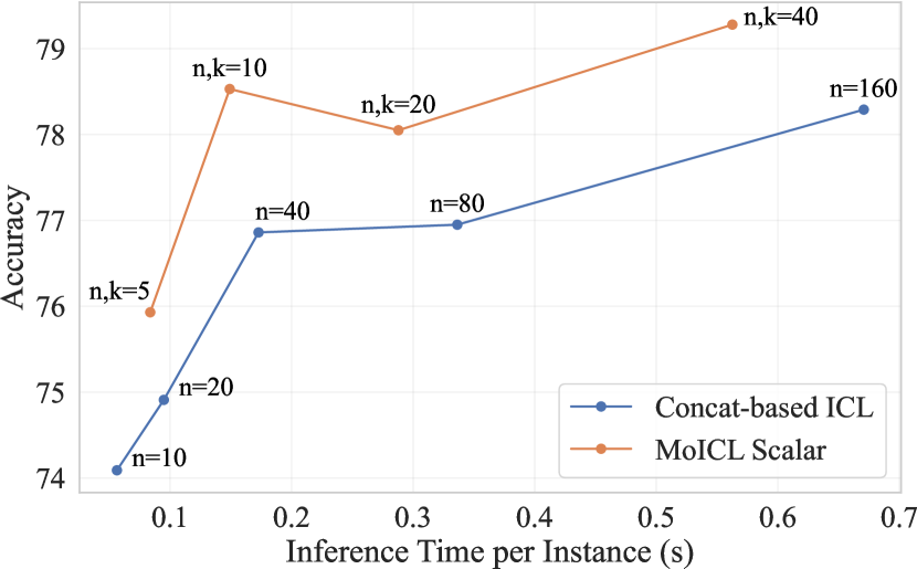
(a) TweetEval Offensive

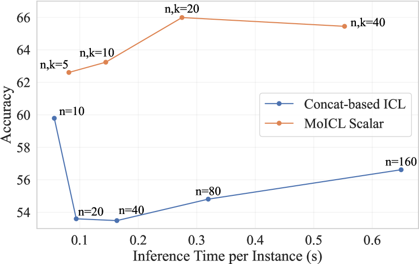
(b) TweetEval Hate

Figure 6: An analysis of the inference time efficiency of MoICL on the TweetEval offensive/hate test set using Llama-3-8B-Instruct. The total number of demonstrations available to MoICL scalar is 160, the same as the maximum number of demonstrations that concat-based ICL can use within the context length limit.

Furthermore, we also analysed whether MoICL could be more time-efficient compared to concat-based ICL under the same settings.  Fig. 6 compares the performance in terms of the average inference time (in seconds) per instance when up to 160 annotated demonstrations (which is the context length limit for concat-based ICL) are provided. We observed that MoICL consistently showed higher accuracy compared to concat-based ICL relative to inference time, demonstrating that MoICL is not only data-efficient but also time-efficient.

Method	Complexity
Concat-based ICL	$(n+1)^{2}\cdot C_{\text{LLM}}$
Ensemble-based ICL	$n\cdot(1+1)^{2}\cdot C_{\text{LLM}}$
Mixture of ICL
- uniform	$k\cdot(\frac{n}{k}+1)^{2}\cdot C_{\text{LLM}}$
- scalar	$k\cdot(\frac{n}{k}+1)^{2}\cdot C_{\text{LLM}}$
- Hyper-network	$k\cdot(\frac{n}{k}+1)^{2}\cdot C_{\text{LLM}}+n^{2}\cdot C_{\text{Hyper}}$

Table 9: Comparison of the computational complexity at inference time between MoICL Methods and Baseline ICL Methods. $C_{\text{LLM}}$ and $C_{\text{Hyper}}$ refer to the unit computation complexity for one demonstration and one forward pass for an LLM and Hyper-network, respectively. $n$ and $k$ refer to the number of demonstrations and the number of subsets.

Complexity

The proposed MoICL method partitions demonstrations into subsets rather than concatenating them, thereby reducing the input context length for LLMs. This reduction is beneficial in Transformer-based architectures, where computational load increases quadratically with the context length. In Table 9, we analyse the computation cost based on the unit computation cost (one forward pass for one example) of LLM and Hyper-network, namely $C_{\text{LLM}}$ and $C_{\text{Hyper}}$.

Concat-based ICL exhibits the highest cost by concatenating all demonstrations and the test input $(n+1)$, whereas Ensemble-based ICL shows the lowest cost by concatenating each demonstration with the test input $(1+1)$. MoICL lies in-between, with the cost determined by the number of subsets, $k$. Hyper-network takes all subsets as input and outputs the weight for each subset, thereby adding a cost of $(n+1)^{2}\cdot C_{\text{Hyper}}$. Since $C_{\text{LLM}}$ is usually much larger than $C_{\text{Hyper}}$, this approach still offers a computational advantage. Furthermore, the weights of the subsets only need to be computed once and can be reused for future inputs, which means $n^{2}\cdot C_{\text{Hyper}}$ is a one-time process.

6 Related Work

In-Context Learning

In-context learning (ICL) is an approach to few-shot learning by concatenating the training examples and providing them as input to the model before the actual test example. Being able to perform ICL is an emerging ability of very large models, such as GPT-3 (Brown et al., 2020) and PaLM (Chowdhery et al., 2023). One characteristic of ICL is that increasing the number of demonstrations tends to increase the downstream task accuracy (Brown et al., 2020; Lu et al., 2022). However, Agarwal et al. (2024) show that, after a given number of demonstrations, performance saturates and additional examples might even decrease the downstream task accuracy. Furthermore, in Transformer-based LLMs, increasing the number of ICL demonstrations can be too computationally demanding due to the complexity of self-attention operations growing quadratically with the context size (Liu et al., 2022). Finally, ICL is sensitive to out-of-domain demonstrations (Min et al., 2022b) or label imbalance, underscoring the importance of the selection of the in-context demonstrations to use (Zhao et al., 2021; Fei et al., 2023).

Ensembles of Demonstrations

Min et al. (2022a) introduce ensemble-based demonstrations as an alternative to concat-based ICL (Section 2.1), where each demonstration $(x_{i},y_{i})$ is provided to a language model along with the input $x$ to obtain a next-token distribution $p\left(y\mid x_{i},y_{i},x\right)$; such next-token distributions are then combined in a product-of-experts to produce the final next-token distribution: $p\left(y\mid x_{1},y_{1},\ldots,x\right)=\prod_{i}p\left(y\mid x_{i},y_{i},x\right)$. Le et al. (2022) propose Mixtures of In-Context Experts for anaphora resolution, where the weights for each expert were calculated based on the cosine similarity between the embeddings of the test input and the demonstrations. Ye et al. (2023) extend the models by Le et al. (2022) and analyse the impact of merging the expert activations at different stages, both in terms of efficiency and downstream task performance.

Our proposed Mixture of In-Context Learners (MoICL) extends such approaches by learning a weighting function assigning specific weights to each expert. Our experiments show that this approach allows us to tackle various challenges in ICL (such as label imbalance, out-of-distribution demonstrations, and sample selection) without requiring access to the model weights.

7 Conclusions

We proposed Mixture of In-Context Learners (MoICL), a method for dynamically learning to combine multiple models, each trained via ICL, via gradient-based optimisation methods. We show that MoICL significantly improves accuracy compared to a set of strong baselines. Furthermore, we show that MoICL is robust to out-of-domain and noisy demonstrations, can help mitigate label imbalance, and can be used for selecting sets of demonstrations.

Limitations

Although MoICL does not require direct access to the model parameters, it requires access to the logits of the distribution over the vocabulary or answers produced by the model, both to train the experts and to calculate the final prediction at inference time, which prevents its use with black-box models like GPT-4. Future work can consider black-box optimisation methods to address this limitation.

An important direction for future work, though not explored in this study, is extending the learned weights to the demonstrations across the entire training set. Currently, we sample $n$ demonstrations from the training set and assign them to experts, tuning their weights. Extending this to all demonstrations in the training set would require progressively expanding the experts and their tuned weights. One possible approach for future work is to incorporate the search and relevance heuristics proposed by Li and Qiu (2023) as inductive biases in our proposed hyper-network.

Additionally, due to computational resource limitations, we conducted our experiments on the Llama-2 models (Llama-2-7B-chat, Llama-2-13B-chat, Llama-2-70B-chat) and Llama-3 models (Llama-3-8B, Llama-3-8B-Instruct) as target LLMs, and T5-models (T5-efficient-tiny, T5-efficient-mini, T5-small, T5-base) as hyper-networks. However, our method is not limited to specific LMs and can be applied across various models.

Acknowledgments

Giwon Hong was supported by the ILCC PhD program (School of Informatics Funding Package) at the University of Edinburgh, School of Informatics. Pasquale Minervini and Emile van Krieken were partially funded by ELIAI (The Edinburgh Laboratory for Integrated Artificial Intelligence), EPSRC (grant no. EP/W002876/1). Additionally, Pasquale Minervini was partially funded by an industry grant from Cisco, and a donation from Accenture LLP. This work was supported by the Edinburgh International Data Facility (EIDF) and the Data-Driven Innovation Programme at the University of Edinburgh.

Split	Offensive	Hate	SST2	RTE	FEVER	PAWS	QNLI
Train set	11,916	9,000	66,349	2,190	54,550	49,401	99,743
Dev set	1,324	1,000	1,000	300	5,000	8,000	5,000
Test set	860	2,970	872	277	13,332	8,000	5463

Table 10: Statistics of the classification datasets used in our experiments.

Appendix A Detailed Experiment Settings

A.1 Datasets

TweetEval (Barbieri et al., 2020) offensive/hate datasets are originally from Zampieri et al. (2019) and  Basile et al. (2019), respectively. PAWS (Zhang et al., 2019) is released under a custom license from Google LLC. For SST-2 (Socher et al., 2013), RTE (Bentivogli et al., 2009), FEVER (Thorne et al., 2018), and QNLI (Wang et al., 2018), we used the original validation/development set as the test set and sampled a portion of the training set to construct a new validation set.  Table 10 presents the dataset split statistics for all classification datasets used in our experiments. For NQ-open (Lee et al., 2019), we used the top 1 retrieved documents as a context. The dataset contains 79,168 train instances, 8,757 validation instances, and 3,610 test instances.

A.2 Hyperparameters

We used five seeds $[31,42,65,438,991]$ in all experiments except for NQ-open, which were applied to every possible aspect, including dataset shuffle, demonstration pooling and partition, and Hyper-network fine-tuning, and baseline results. For NQ-open, we only use seed 42. Also, we set the batch size to 1, the gradient accumulation steps to 12 and the learning rate to 0.0001, without performing a hyperparameter search for these settings. For the PEFT  (LoRA, Hu et al., 2022) baseline, we set $r$=16 (rank), alpha=32 (scale factor), and dropout=0.1. We did not perform a search for these LoRA hyperparameters as we utilised the default settings provided by Mangrulkar et al. (2022). Unless otherwise specified, a total of 30 demonstrations were used along with Static partitioning. Both scalar and Hyper-network were tuned for 5 epochs.

For the data efficiency analysis on Fig. 5 in Section 5, we applied the same training step (10,240) to all different MoICL settings.

A.3 Implementation Details

MoICL

For all datasets used in the experiments, we fine-tuned all the MoICL weights and hyper-network on the training set and evaluated them on the validation/development set at each epoch, selecting the ones with the highest performance. The results reported in all experiments were measured on the test set. For scalar, we first sampled $D$ from the training set based on the different seeds and used the remaining training instances as $D_{T}$ (Section 2.2). For hyper-network, $D$ is not available during training and is used only during evaluation. We further separate $D_{T}$ into $D_{pool}$ and $D_{pair}$ randomly at each epoch, where demonstrations are sampled from $D_{pool}$ and $(x,y)\in D_{pair}$. While any model that produces weights can be used for the hyper-network, we attach a linear layer on top of a pre-trained encoder-decoder T5-small (Raffel et al., 2020) model.

Baselines

For PEFT fine-tuned on RTE, we applied early stopping based on the dev set accuracy, as we observed that the training process was highly unstable. Both Ensemble-based ICL (Min et al., 2022a) and LENS Li and Qiu (2023) used the Direct method instead of the Channel method, which also applied for MoICL as well. For LENS, We first apply Progressive Example Filtering to select 30 demonstrations, then perform Diversity-Guided Search to obtain 5 permutations of the examples, and report the average and standard deviation based on these 5 permutations.

Appendix B Additional Analyses

B.1 Partitioning a Demonstration set $D$.

In this work, we analyse the following partitioning strategies: Static, Random Size, and BM25. Static means partitioning $n$ demonstrations into $k$ subsets, with each subset containing $n/k$ demonstrations. Random Size refers to partitioning into $k$ subsets, each containing a random number of elements. BM25 apply $k$-NN clustering based on BM25 scores on demonstrations (Robertson et al., 2009) to partition into them $k$ subsets.

MoICL Method	Static	Random Size	BM25
uniform
$k=3$	74.86$\pm$1.84	74.74$\pm$1.90	74.79$\pm$1.79
$k=5$	73.77$\pm$1.60	74.09$\pm$1.35	73.47$\pm$2.19
$k=10$	74.00$\pm$0.87	73.37$\pm$0.94	74.40$\pm$0.82
scalar
$k=3$	76.14$\pm$1.48	77.37$\pm$1.97	77.21$\pm$2.02
$k=5$	78.35$\pm$1.49	77.67$\pm$2.69	78.37$\pm$1.62
$k=10$	79.42$\pm$1.48	78.72$\pm$0.87	79.70$\pm$1.32

Table 11: Analysis of partitioning methods. Random and BM25 represent random clustering and clustering based on BM25 scores, respectively. Bold text signifies the highest accuracy for each method.

Table 11 compares the performance of MoICL methods and different partitioning methods (Static, Random, BM25) for the same $k$ (number of subsets). In uniform, there is little difference between Static and Random and only a slight performance improvement with BM25. However, there is a common performance enhancement when MoICL scalar are applied. This indicates that our proposed method is not significantly affected by partitioning methods and can be applied in a complementary manner across them. As such, we decided to use only the Static method in the other experiments.

B.2 Logits vs. Probabilities for Mixing Experts

As stated in Section 2.2, we mix the experts in the log domain. However, it is also possible—and perhaps more appropriate—to use a regular mixture of probabilities, as in Eq. 5.

$$p\left(y\mid D,x\right)\propto\left[\sum_{i=1}^{k}w_{i}p\left(y\mid D_{i},x\right)\right]$$ (5)

Accordingly, in Fig. 2, we compare the accuracy trends based on partitioning size when using weighting in the probability and logit domains. In uniform, whether logits or probabilities were used did not make a significant difference, but in scalar, the impact was substantial. This is likely because distinct differences in the distribution patterns among experts (and thus useful information in the mixture) get diluted during the normalisation process when using probabilities.

B.3 MoICL in a Generation Task

Methods ($n=12$)	NQ-open (EM)
Concat-based ICL	0.4083
Ensemble-based ICL (Min et al., 2022a)	0.3753
Random Search	0.4008
Mixture of ICL (uniform)
$k=6$	0.3864
$k=12$	0.3753
Mixture of ICL (uniform)
$k=6$	0.3861
$k=12$	0.3742
Mixture of ICL (Hyper-network)
$k=6$	0.3848
$k=12$	0.3842

Table 12: Comparison between baseline methods and MoICL on NQ-open using Llama-3-8B. $k$ represents the number of demonstrations subset, where the total number of demonstrations ($n$) is 12

In addition to the classification tasks in  Section 4.1, we also apply our MoICL on a generation task, NQ-open (Lee et al., 2019), in  Table 12. However, unlike in classification tasks, MoICL did not show significant EM improvements over baseline approaches. Nevertheless, as seen in  Section 4.6, MoICL exhibited strong robustness in situations involving noised demonstrations, proving the usefulness of the expert’s tuned weights.

Appendix C Prompt Templates

Table 13 presents the corresponding metric and prompt template for all tasks included in the experiments. For NQ, CNN/DM, and XSum, the delimiter for ICL demonstrations was ‘\n\n’. For the remaining tasks, ‘\n’ was used as the delimiter.

Table 13: Prompt template setting details for the tasks. The double curly braces "{{}}" signify input data.

Task	Metric	Prompt Template
TweetEval Offensive	Accuracy	Classify tweets that are offensive as offensive, and tweets that are not offensive as neutral. {{ICL Demonstrations}} Tweet: {{tweet}} Label:
TweetEval Hate	Accuracy	Classify tweets that are hateful against immigrants or women as hate and tweets that are not hateful against immigrants or women as neutral. {{ICL Demonstrations}} Tweet: {{tweet}} Label:
SST2	Accuracy	Classify sentences that are negative as negative and sentences that are positive as positive. {{ICL Demonstrations}} Sentence: {{sentence}} Label:
RTE	Accuracy	Classify two sentences that entail each other as true and two sentences that do not entail each other as false. {{ICL Demonstrations}} Sentence1: {{first sentence}} Sentence2: {{second sentence}} Label:
FEVER	Accuracy	Classify claims that are false as refuted, and tweets that are true as supported. {{ICL Demonstrations}} Claim: {{claim}} Label:
PAWS	Accuracy	Classify the two sentences as yes if they are paraphrases of each other, and if not, classify them as no. {{ICL Demonstrations}} sentence1: {{first sentence}} sentence2: {{second sentence}} label:
QNLI	Accuracy	Classify as yes if the sentence contains the answer to the question, if not, classify as no. {{ICL Demonstrations}} sentence: {{sentence}} question: {{question}} label:
NQ	EM	{{ICL Demonstrations}} title: {{title}} text: {{text}} Question: {{question}} Answer:

Appendix D Computation Details

The experiments were conducted using NVIDIA A100 40GBs and 80GBs with 120GB of RAM. The GPU hours vary depending on the models and tasks; tuning MoICL scalar weights ($n,k=30$) on TweetEval offensive takes approximately 1 hour and 20 minutes per epoch.

References

- Agarwal et al. (2024) Rishabh Agarwal, Avi Singh, Lei M Zhang, Bernd Bohnet, Luis Rosias, Stephanie CY Chan, Biao Zhang, Aleksandra Faust, and Hugo Larochelle. 2024. Many-shot in-context learning. In ICML 2024 Workshop on In-Context Learning.
- AI@Meta (2024) AI@Meta. 2024. Llama 3 model card.
- Barbieri et al. (2020) Francesco Barbieri, Jose Camacho-Collados, Luis Espinosa Anke, and Leonardo Neves. 2020. TweetEval: Unified benchmark and comparative evaluation for tweet classification. In Findings of the Association for Computational Linguistics: EMNLP 2020, pages 1644–1650, Online. Association for Computational Linguistics.
- Basile et al. (2019) Valerio Basile, Cristina Bosco, Elisabetta Fersini, Debora Nozza, Viviana Patti, Francisco Manuel Rangel Pardo, Paolo Rosso, and Manuela Sanguinetti. 2019. SemEval-2019 task 5: Multilingual detection of hate speech against immigrants and women in Twitter. In Proceedings of the 13th International Workshop on Semantic Evaluation, pages 54–63, Minneapolis, Minnesota, USA. Association for Computational Linguistics.
- Bentivogli et al. (2009) Luisa Bentivogli, Peter Clark, Ido Dagan, and Danilo Giampiccolo. 2009. The fifth pascal recognizing textual entailment challenge. TAC, 7(8):1.
- Brown et al. (2020) Tom Brown, Benjamin Mann, Nick Ryder, Melanie Subbiah, Jared D Kaplan, Prafulla Dhariwal, Arvind Neelakantan, Pranav Shyam, Girish Sastry, Amanda Askell, Sandhini Agarwal, Ariel Herbert-Voss, Gretchen Krueger, Tom Henighan, Rewon Child, Aditya Ramesh, Daniel Ziegler, Jeffrey Wu, Clemens Winter, Chris Hesse, Mark Chen, Eric Sigler, Mateusz Litwin, Scott Gray, Benjamin Chess, Jack Clark, Christopher Berner, Sam McCandlish, Alec Radford, Ilya Sutskever, and Dario Amodei. 2020. Language models are few-shot learners. In Advances in Neural Information Processing Systems, volume 33, pages 1877–1901. Curran Associates, Inc.
- Chen et al. (2023) Yanda Chen, Chen Zhao, Zhou Yu, Kathleen McKeown, and He He. 2023. On the relation between sensitivity and accuracy in in-context learning. In 2023 Findings of the Association for Computational Linguistics: EMNLP 2023, pages 155–167. Association for Computational Linguistics (ACL).
- Chowdhery et al. (2023) Aakanksha Chowdhery, Sharan Narang, Jacob Devlin, Maarten Bosma, Gaurav Mishra, Adam Roberts, Paul Barham, Hyung Won Chung, Charles Sutton, Sebastian Gehrmann, Parker Schuh, Kensen Shi, Sasha Tsvyashchenko, Joshua Maynez, Abhishek Rao, Parker Barnes, Yi Tay, Noam Shazeer, Vinodkumar Prabhakaran, Emily Reif, Nan Du, Ben Hutchinson, Reiner Pope, James Bradbury, Jacob Austin, Michael Isard, Guy Gur-Ari, Pengcheng Yin, Toju Duke, Anselm Levskaya, Sanjay Ghemawat, Sunipa Dev, Henryk Michalewski, Xavier Garcia, Vedant Misra, Kevin Robinson, Liam Fedus, Denny Zhou, Daphne Ippolito, David Luan, Hyeontaek Lim, Barret Zoph, Alexander Spiridonov, Ryan Sepassi, David Dohan, Shivani Agrawal, Mark Omernick, Andrew M. Dai, Thanumalayan Sankaranarayana Pillai, Marie Pellat, Aitor Lewkowycz, Erica Moreira, Rewon Child, Oleksandr Polozov, Katherine Lee, Zongwei Zhou, Xuezhi Wang, Brennan Saeta, Mark Diaz, Orhan Firat, Michele Catasta, Jason Wei, Kathy Meier-Hellstern, Douglas Eck, Jeff Dean, Slav Petrov, and Noah Fiedel. 2023. Palm: Scaling language modeling with pathways. J. Mach. Learn. Res., 24:240:1–240:113.
- Fei et al. (2023) Yu Fei, Yifan Hou, Zeming Chen, and Antoine Bosselut. 2023. Mitigating label biases for in-context learning. In Proceedings of the 61st Annual Meeting of the Association for Computational Linguistics (Volume 1: Long Papers), pages 14014–14031, Toronto, Canada. Association for Computational Linguistics.
- Ha et al. (2017) David Ha, Andrew M. Dai, and Quoc V. Le. 2017. Hypernetworks. In ICLR (Poster). OpenReview.net.
- Hu et al. (2022) Edward J Hu, Yelong Shen, Phillip Wallis, Zeyuan Allen-Zhu, Yuanzhi Li, Shean Wang, Lu Wang, and Weizhu Chen. 2022. LoRA: Low-rank adaptation of large language models. In International Conference on Learning Representations.
- Kwiatkowski et al. (2019) Tom Kwiatkowski, Jennimaria Palomaki, Olivia Redfield, Michael Collins, Ankur Parikh, Chris Alberti, Danielle Epstein, Illia Polosukhin, Jacob Devlin, Kenton Lee, et al. 2019. Natural questions: a benchmark for question answering research. Transactions of the Association for Computational Linguistics, 7:453–466.
- Le et al. (2022) Nghia T. Le, Fan Bai, and Alan Ritter. 2022. Few-shot anaphora resolution in scientific protocols via mixtures of in-context experts. In Findings of the Association for Computational Linguistics: EMNLP 2022, pages 2693–2706, Abu Dhabi, United Arab Emirates. Association for Computational Linguistics.
- Lee et al. (2019) Kenton Lee, Ming-Wei Chang, and Kristina Toutanova. 2019. Latent retrieval for weakly supervised open domain question answering. In Proceedings of the 57th Annual Meeting of the Association for Computational Linguistics, pages 6086–6096, Florence, Italy. Association for Computational Linguistics.
- Li and Qiu (2023) Xiaonan Li and Xipeng Qiu. 2023. Finding support examples for in-context learning. In Findings of the Association for Computational Linguistics: EMNLP 2023, pages 6219–6235.
- Liu et al. (2024) Alisa Liu, Xiaochuang Han, Yizhong Wang, Yulia Tsvetkov, Yejin Choi, and Noah A. Smith. 2024. Tuning language models by proxy. In First Conference on Language Modeling.
- Liu et al. (2022) Haokun Liu, Derek Tam, Mohammed Muqeeth, Jay Mohta, Tenghao Huang, Mohit Bansal, and Colin Raffel. 2022. Few-shot parameter-efficient fine-tuning is better and cheaper than in-context learning.
- Lu et al. (2022) Yao Lu, Max Bartolo, Alastair Moore, Sebastian Riedel, and Pontus Stenetorp. 2022. Fantastically ordered prompts and where to find them: Overcoming few-shot prompt order sensitivity. In Proceedings of the 60th Annual Meeting of the Association for Computational Linguistics (Volume 1: Long Papers), pages 8086–8098, Dublin, Ireland. Association for Computational Linguistics.
- Lu et al. (2024) Yao Lu, Jiayi Wang, Raphael Tang, Sebastian Riedel, and Pontus Stenetorp. 2024. Strings from the library of babel: Random sampling as a strong baseline for prompt optimisation. In NAACL-HLT, pages 2221–2231. Association for Computational Linguistics.
- Mangrulkar et al. (2022) Sourab Mangrulkar, Sylvain Gugger, Lysandre Debut, Younes Belkada, Sayak Paul, and Benjamin Bossan. 2022. Peft: State-of-the-art parameter-efficient fine-tuning methods. https://github.com/huggingface/peft.
- Min et al. (2022a) Sewon Min, Mike Lewis, Hannaneh Hajishirzi, and Luke Zettlemoyer. 2022a. Noisy channel language model prompting for few-shot text classification. In Proceedings of the 60th Annual Meeting of the Association for Computational Linguistics (Volume 1: Long Papers), pages 5316–5330, Dublin, Ireland. Association for Computational Linguistics.
- Min et al. (2022b) Sewon Min, Xinxi Lyu, Ari Holtzman, Mikel Artetxe, Mike Lewis, Hannaneh Hajishirzi, and Luke Zettlemoyer. 2022b. Rethinking the role of demonstrations: What makes in-context learning work? In Proceedings of the 2022 Conference on Empirical Methods in Natural Language Processing, pages 11048–11064, Abu Dhabi, United Arab Emirates. Association for Computational Linguistics.
- Minervini et al. (2023) Pasquale Minervini, Luca Franceschi, and Mathias Niepert. 2023. Adaptive perturbation-based gradient estimation for discrete latent variable models. In AAAI, pages 9200–9208. AAAI Press.
- Niepert et al. (2021) Mathias Niepert, Pasquale Minervini, and Luca Franceschi. 2021. Implicit mle: backpropagating through discrete exponential family distributions. Advances in Neural Information Processing Systems, 34:14567–14579.
- Raffel et al. (2020) Colin Raffel, Noam Shazeer, Adam Roberts, Katherine Lee, Sharan Narang, Michael Matena, Yanqi Zhou, Wei Li, and Peter J. Liu. 2020. Exploring the limits of transfer learning with a unified text-to-text transformer. Journal of Machine Learning Research, 21(140):1–67.
- Robertson et al. (2009) Stephen Robertson, Hugo Zaragoza, et al. 2009. The probabilistic relevance framework: Bm25 and beyond. Foundations and Trends® in Information Retrieval, 3(4):333–389.
- Socher et al. (2013) Richard Socher, Alex Perelygin, Jean Wu, Jason Chuang, Christopher D. Manning, Andrew Ng, and Christopher Potts. 2013. Recursive deep models for semantic compositionality over a sentiment treebank. In Proceedings of the 2013 Conference on Empirical Methods in Natural Language Processing, pages 1631–1642, Seattle, Washington, USA. Association for Computational Linguistics.
- Thorne et al. (2018) James Thorne, Andreas Vlachos, Christos Christodoulopoulos, and Arpit Mittal. 2018. Fever: a large-scale dataset for fact extraction and verification. In Proceedings of the 2018 Conference of the North American Chapter of the Association for Computational Linguistics: Human Language Technologies, Volume 1 (Long Papers), pages 809–819.
- Touvron et al. (2023) Hugo Touvron, Louis Martin, Kevin Stone, Peter Albert, Amjad Almahairi, Yasmine Babaei, Nikolay Bashlykov, Soumya Batra, Prajjwal Bhargava, Shruti Bhosale, et al. 2023. Llama 2: Open foundation and fine-tuned chat models. arXiv preprint arXiv:2307.09288.
- Voronov et al. (2024) Anton Voronov, Lena Wolf, and Max Ryabinin. 2024. Mind your format: Towards consistent evaluation of in-context learning improvements. In ACL (Findings), pages 6287–6310. Association for Computational Linguistics.
- Wang et al. (2018) Alex Wang, Amanpreet Singh, Julian Michael, Felix Hill, Omer Levy, and Samuel Bowman. 2018. Glue: A multi-task benchmark and analysis platform for natural language understanding. In Proceedings of the 2018 EMNLP Workshop BlackboxNLP: Analyzing and Interpreting Neural Networks for NLP, pages 353–355.
- Wei et al. (2022) Jason Wei, Yi Tay, Rishi Bommasani, Colin Raffel, Barret Zoph, Sebastian Borgeaud, Dani Yogatama, Maarten Bosma, Denny Zhou, Donald Metzler, et al. 2022. Emergent abilities of large language models. Transactions on Machine Learning Research.
- Xu et al. (2024) Xin Xu, Yue Liu, Panupong Pasupat, Mehran Kazemi, et al. 2024. In-context learning with retrieved demonstrations for language models: A survey. arXiv preprint arXiv:2401.11624.
- Ye et al. (2023) Qinyuan Ye, Iz Beltagy, Matthew Peters, Xiang Ren, and Hannaneh Hajishirzi. 2023. FiD-ICL: A fusion-in-decoder approach for efficient in-context learning. In Proceedings of the 61st Annual Meeting of the Association for Computational Linguistics (Volume 1: Long Papers), pages 8158–8185, Toronto, Canada. Association for Computational Linguistics.
- Zampieri et al. (2019) Marcos Zampieri, Shervin Malmasi, Preslav Nakov, Sara Rosenthal, Noura Farra, and Ritesh Kumar. 2019. Semeval-2019 task 6: Identifying and categorizing offensive language in social media (offenseval). In Proceedings of the 13th International Workshop on Semantic Evaluation, pages 75–86.
- Zhang et al. (2019) Yuan Zhang, Jason Baldridge, and Luheng He. 2019. PAWS: Paraphrase adversaries from word scrambling. In Proceedings of the 2019 Conference of the North American Chapter of the Association for Computational Linguistics: Human Language Technologies, Volume 1 (Long and Short Papers), pages 1298–1308, Minneapolis, Minnesota. Association for Computational Linguistics.
- Zhao et al. (2021) Zihao Zhao, Eric Wallace, Shi Feng, Dan Klein, and Sameer Singh. 2021. Calibrate before use: Improving few-shot performance of language models. In International conference on machine learning, pages 12697–12706. PMLR.