The formulation presented in Section LABEL:bncrpptu:sec:rpptucgf models Rural Postman Problem with Temporal Unavailability (RPP-TU) with binary spatial variables and continuous (non-negative real) temporal variables. We propose a branch-and-cut algorithm that evaluates an upper and a lower bounds of an optimal solution at every node, by solving iteratively modified versions of the formulation for RPP-TU. At each node, these modifications made to the formulation are generated by reducing the feasible region using additional constraints, and then relaxing all the remaining binary variables.

In this subsection, we first discuss the branching strategy to exhaustively obtain all possible solutions to the spatial sub-problem of the presented formulation (binary variables only). Next, we discuss the iteratively modified versions of this formulation, solved at each node of the branch-and-cut algorithm, to improve the upper and lower bound computations. A pseudo-code is provided with a step-wise explanation, along with a separation algorithm for implementing a family of valid inequalities as cutting-planes. Lastly, the polyhedral properties of the RPP-TRU are studied to establish that the proposed cutting-planes are facet-defining.

0.1 Branching over service arcs

The philosophy of branching is to implement an exhaustive search for an optimal solution in a finite set, hence terminating at the exact solution. The spatial problem of the formulation (denoted as $F_{X}$) is binary programming and hence composed of a finite number of feasible solutions. One approach for implementing a branching strategy, in a single-agent case, is by generating one child node for each available service arc, as presented in [calogiuri]. However, the branching strategy in multi-agent problems is not as direct. In this subsection, we introduce a procedure to branch over service arcs of a layered graph that addresses a multi-agent routing problem.

Branches

At each parent node, one branch is assigned for each available service arc to only one agent, and one extra branch is added to represent no assignment of service arcs to this agent (i.e. another agent will be involved next). In particular, excluding the extra branch, all other branches are assigned for each available (previously unassigned) service arc in a layer (starting from the smallest layer in $\mathcal{L}$) to only one agent (preferred based on fractional solution of $F_{X}$). Figure 1 shows $3$ generations of exhaustive branching for the example problem from [lannez] (the example graph is shown in Figure LABEL:fig:prelim_fig2) whose replicated graph is shown in Figure LABEL:fig:prelim_fig3 for $3$ agent case. Note that, in a replicated graph, if all service arc of a particular layer of agent-sub-graph are unassigned, then no succeeding layers can be assigned to this agent i.e. this agent is not available for further assignment.

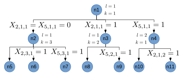
justification=centering

Figure 1: Illustration of branching for example graph in Figure LABEL:fig:prelim_fig2. At node $n1$, the branching is done for $l=1,k=1$; resulting in three child nodes with binary restrictions shown at the connecting branches. Assuming fractional solution is observed in $X_{2,3,1}$, the branching at node $n_{2}$ is performed for $l=1,k=3$. Similarly, assuming that fractional solution is observed in $X_{5,2,2}$, node $n3$ is evaluated for $l=1,k=2$ (no branching for arc $a_{2}$ as it has already been assigned in its parent node). If no fractional solution is achieved (say at node $n4$), then a new layer is explored for the same agent-sub-graph i.e. $l=1,k=1$.

The objective of branching is to eliminate fractional solutions, hence the branching is performed on the smallest unassigned layer of any of the $|\mathcal{K}|$ agent-sub-graphs with priority for arcs with fractional spatial solution. In other words, if one of the service arcs of the smallest unassigned layers is fractional ($X_{2,3,1}$ at node $n2$ in Figure 1) then branching is performed for this particular layer $l=1$ and agent-sub-graph $k=3$. If none of the service arcs of the smallest unassigned layer of any of the agent-sub-graphs are fractional, then either (a) the spatial solution is completely binary, and hence the branching is performed for any of the service arc of the smallest layer of an available agent-sub-graph ($n4$ in Figure 1); or (b) there are fractional solutions in later layers ($X_{5,2,2}$ at node $n3$ in Figure 1), hence the smallest unused layer $l=1$ of this agent-sub-graph $k=2$ is preferred for branching.

In order to implement this branching strategy, two pieces of information are recorded at every node, (1) list of available service arcs and (2) list of available agents, for evaluating future generations of these nodes. Now, based on our branching strategy, $|A_{*}|+1$ child branches are generated at the root node, if the number of available agents is of size greater than $1$; otherwise there is one less child branch i.e. only $|A_{*}|$ branches at the root node for single-agent case. In particular, the extra branch, representing no assignment of service arcs of a layer, is not generated if the number of available agents is $1$. For each child node, if a service arc has been assigned in the previous generation of branches then the number of branches reduces by one because the list of available service arcs is shortened. If a particular child node is attached to the extra branch where no service arc of a layer was assigned, then this agent is removed from the list of available agents, and the number of child branches is same as the previous generation of branching; provided the list of available agent is of size greater than $1$. Note that, with this strategy, the number of generations in this branch-and-cut algorithm (depth of the branch-and-node search-tree) must be at most $|A_{*}|+|\mathcal{K}|$.

Nodes

The branching strategy iteratively adds nodes to a branch-and-cut search-tree. Some of these nodes are freshly added, and hence have no branches or child nodes in that iteration. These non-evaluated (unsolved) child nodes of the current iteration are also called leaf nodes. At each iteration of the branch-and-cut algorithm, one of the leaf node with the smallest lower bound is selected and evaluated. This evaluation process involves branching to produce child nodes, and solving a modified versions of the formulation for obtaining a lower and upper bound. The modifications are due to binary relaxation, selection of service arcs in previous generations, and some improvement strategies for faster convergence to optimal solution.

The binary relaxations convert the underlying Mixed Integer Linear Programming (MILP) problem at the node to Linear Programming (LP) problem, thus simplifying the computation. Service arc assignment to an agent is useful in reducing the number of decisions, hence further simplifying the problem to be solved at the current node. This reduction in decision variables occur because, once a service arc is selected while branching, the fastest paths to these service arcs are inherently optimal in this scenario. Hence, for each child node of the current node, a fastest path algorithm (shortest path algorithm with running time and unavailability data, using base graph $G$) is solved, and all the arcs involved in this path are forced as $1$. All the iterative modifications are discussed in detail in Subsection 0.2. This subsection also discusses the steps for computation of an upper bound, at the current node. Note that, if the upper bound is larger than or equal to the smallest lower bound among the leaf nodes, the algorithm terminates (optimal solution is achieved).

0.2 Iterative modification of the formulation at the nodes

Each modification of the formulation has spatial and temporal variables, which are solved separately. Observe that, given a spatial binary solution $\bar{X}$, one may substitute it into the running-time and unavailability constraints, given by Equation (LABEL:form:run) and Equation (LABEL:form:unav) respectively, to obtain constraints that depend on temporal variables $\Gamma$ only. Let $\bar{\Gamma}$ be the lowest cost temporal solution for a given binary spatial solution $\bar{X}$, then the cost of the solution $(\bar{X},\bar{\Gamma})$ is set as the upper bound of the optimal solution. In case given $\bar{X}$ is binary but has no feasible temporal solution $\bar{\Gamma}$, or the given $\bar{X}$ is fractional, then the upper bound is set as the parent or the initialized upper bound. The lower bound, in all these cases, is the optimal cost of the spatial sub-problem. This method of solving the spatial and temporal parts separately reduces a larger problem to two smaller sub-problems. Moreover, given spatial solution $\bar{X}$, the either-or representation of unavailability constraints, given by Equation (LABEL:form:unav) becomes non-disjoint. This simplification is observed because one of the either-or constraints is ineffective if the spatial variable is known.

The modifications in the basic formulation framework is contributed by (1) an improvement strategy that leads to better lower and upper bounds, and (2) the branching strategy described earlier that reduces the problem size by allocating decisions to some of the arcs before solving the resulting linear programming problem.

[align=right,labelwidth=0.8cm,leftmargin=1.0cm, labelsep=0.2cm,itemsep=0.9cm]

The improvement strategy is incorporated into the proposed branch-and-cut algorithm to reduce the number of iterations and hence the overall computation time. Cutting-planes derived from a family of proposed valid inequalities is one such strategy. The cutting-planes reduces the number of fractional solutions in the relaxation, thus reducing the number of iterations. The family of valid inequalities used as cutting-planes for $F_{X}$ are given in Theorem 1.

The presented branching strategy introduces another modification to our formulation, which contributes in determining a better lower bound using $|\mathcal{K}|$ additional constraints. These constraints are based on paths generated while assigning service arcs, in the branching process of the parent generations. These paths connects each agent’s source vertex to various service arcs of the agents. Let these paths be denoted by $\mathcal{P}_{k}$, for $k\in\mathcal{K}$. Since all these path starts from the source vertex, the starting time is assumed as zero, and the total delay due to unavailabilities (difference between actual traversal time and the total running time of the paths) are computed greedily using the fastest path algorithm mentioned in the previous subsection. This time value is denoted by $d_{k}$, where $k\in\mathcal{K}$, and the constraints due to these paths are given by Equation (1).

$$\aligned\hat{\gamma}\geq&\sum_{a_{qkl}\in(\mathcal{A}_{R}\cup\mathcal{A}_{l})\backslash\mathcal{P}}W_{q}X_{qkl}\\ +\sum_{a_{qkl}\in\mathcal{P}_{k}}W_{q}+d_{k},\\ \textit{where, }\mathcal{P}=\cup_{k\in\mathcal{K}}\mathcal{P}_{k}$$ (1)

The variable $\hat{\gamma}$ acts as an estimate for the temporal cost, which produces valid lower bounds for fractional spatial solutions also. Note that, if the entire path of an agent from source to sink vertex is given, then the lower bound computed by the spatial-problem is same as the total cost (spatial cost $+$ temporal cost) of the solution.

Evidently, the temporal sub-problem is expressed as:

$$\tag{P_{T}}\aligned\underset{}{\text{min}}&\gamma\\ \text{s.t.}\textit{Equation (\ref{form:cost}), Equation (\ref{form:run}) and }\\ ~{}~{}\textit{Equation (\ref{form:unav})}\\ \textit{given $X$ from the spatial }\\ ~{}~{}\textit{ sub-problem }\\ \Gamma\geq 0$$

Similarly, the spatial-problem to be solved in each branch-and-cut iteration is of the form:

$$\tag{P_{S}}\aligned\underset{}{\text{min}}&\sum_{a_{qkl}\in(\mathcal{A}_{R}\cup\mathcal{A}_{l})\backslash\mathcal{P}}W_{q}X_{qkl}+\hat{\gamma}\\ \text{s.t.}\textit{Equations (\ref{form:flow})-(\ref{form:serv}) }\\ \textit{cutting-planes introduced iteratively }\\ \textit{branching constraints introduced }\\ ~{}~{}\textit{ iteratively }\\ \textit{temporal cost estimate $\hat{\gamma}$ given in }\\ ~{}~{}\textit{ Equation (\ref{eqn:lb}) updated iteratively }\\ 0\leq X_{qkl}\leq 1,\forall a_{qkl}\in(\mathcal{A}_{R}\cup\mathcal{A}_{l})\backslash\mathcal{P}\\$$

The temporal sub-problem is only evaluated if the corresponding spatial sub-problem produces binary solution and its spatial cost is smaller than the current upper bound.

0.3 Pseudo-code for the proposed branch-and-cut method

Algorithm 0.3 shows a pseudo-code to implement the proposed branch-and-cut method. Cost and constraint matrices of the presented formulation are input to the algorithm, while the output is an optimal solution. The search-tree is initialized with the input problem formulation as root node, and correspondingly, an entry of $-\infty$ is added to a queue recording lower bound of the leaf nodes, called lbLeafNodes. At each node of the search-tree, data is recorded, e.g. upper bound (initialized using parent upper bound), spatial and temporal solutions (initialized as empty), forced integer variables (due to branching), parent node identity, etc. The best upper bound $ub_{best}$, and the valid inequalities are stored as common data, and updated iteratively. After adding the root node, the algorithm enters a loop which is composed of eight steps $S1-S8$ in sequence unless specified.

[align=right,labelwidth=0.7cm,leftmargin=0.9cm, labelsep=0.2cm,itemsep=0.1cm]

S1.

The first step $S1$ picks the lowest entry in lbLeafNodes which is indicative of the best lower bound so far, using function LoadNodeWithSmallestLB. A breaking condition is also added in this step using function BreakingCondition, which terminates the search if the duality gap between the best upper bound $ub_{best}$ and best lower bound in lbLeafNodes is zero.

S2.

In step $S2$, the relaxation problem 0.2 is solved using function SolveLPrelaxation, and the corresponding search-tree data is updated, including updating the corresponding entry in lbLeafNodes as $\infty$ to avoid re-selection in step $S1$. This update also ensures that the best lower bound mentioned in $S1$ is a non-decreasing function.

S3.

Next, in step $S3$, if this lower bound is larger than the best upper bound $ub_{best}$, the algorithm returns to step $S1$ for re-selection of a better node, otherwise it jumps to next step.

S4.

The spatial solution is checked for fractional terms in step $S4$. In case its an all integer spatial solution, the algorithm moves to step $S5$, otherwise the algorithm jumps to step $S7$ to search for valid inequalities.

S5.

In step $S5$, a temporal solution is computed using (0.2), and an upper bound (the true spatio-temporal cost of the solution) is also generated, as shown by function SolveForUB. If a temporal solution doesn’t exist for this spatial solution, then its upper bound is set as the parent upper bound.

S6.

For the feasible temporal solution scenario, if the upper bound is smaller than the best upper bound $ub_{best}$, then the $ub_{best}$ is replaced in step $S6$, otherwise it jumps to step $S8$ for branching.

S7.

In the next step $S7$, valid inequalities are identified using function FindCuts, also see Algorithm 1. If found, the algorithm jumps to step $S1$ to re-evaluate the relaxation problem, otherwise branch nodes are generated in step $S8$.

S8.

This branching step $S8$ is evaluated irrespective of the spatial solution being fractional or purely integer, using function GenerateChildNodes. Preference is given to fractional service arcs or agent-sub-graph with fractional arcs, in that order. The details of the branching strategy has been described in Subsection 0.1.

1.05 mycommfont Continuecontinue solverelaxnSolveLPrelaxation isintgrIsAllInteger solvubSolveForUB getleafindxLoadNodeWithSmallestLB lookforcutsSeparationAlgorithm optfoundBreakingCondition genBranchesGenerateChildNodes validcutsFindCuts Inputinput InOut Outputoutput $P$ (An MILP formulation for RPP-TU), $X_{opt},\Gamma_{opt}$ Initialize $T\leftarrow P$ *add the formulation problem to search tree as root node $\textit{vcuts}\leftarrow\emptyset$ *all discovered valid cuts $\textit{lbLeafNodes}\leftarrow-\infty$ *to store lower bound of all branch-and-cut nodes $ub_{best}\leftarrow\infty$ *best upper bound Main loop lbLeafNodes is not entirely infinity S1: Pick the best leaf node from $T$, and check if optimal is found $P,\textit{lbLeafNodes}\leftarrow$ (lbLeafNodes)   ($lbLeafNodes,ub_{best}$) *$ub_{best}$ is at least as large as the current best lower bound $min(lbLeafNodes)$ S2: Solve the relaxation problem and set corresponding lbLeafNodes as infinity $lb,X,T,\textit{lbLeafNodes}\leftarrow$ (lbLeafNodes)   S3: Check if $lb$ of the current node is worth processing $lb\geq ub_{best}$ *goto Step $S1$ S4: Check if all spatial variables in $X$ are integers ($X$) S5: Compute upper bound and temporal solution $ub,\Gamma\leftarrow$($P$)  S6: Update optimal solution and $ub_{best}$ $ub\leq ub_{best}$ $ub_{best}\leftarrow ub$  $X_{opt},\Gamma_{opt}\leftarrow X,\Gamma$ S7: Find cutting-planes and add to tree $T$ $T,\textit{lbLeafNodes},\textit{vcuts}\leftarrow$ ($T,\textit{lbLeafNodes},\textit{vcuts},P,X,lb$) *see Algorithm 1 new valid inequalities are found *goto Step $S1$ S8: Select an agent and generate child nodes for each service arc in the smallest available layer $T,\textit{lbLeafNodes}\leftarrow$ ($P,\textit{lbLeafNodes}$) *add child nodes in tree $T$, and corresponding leaf nodes using parent lower bound crpptu; A branch-and-cut algorithm for RPP-TU

Separation algorithm

The number of branch exploration is reduced by adding cutting-planes to eliminate one or more fractional solutions from the LP relaxation of the current branch-and-cut node. Since this family of inequalities is exponentially large, a valid inequality is selected as a cutting plane only if a violation is identified. This violation of the cutting plane is implemented using a separation algorithm. The family of valid inequalities used in this work are stated in Theorem 1.

Theorem 1.

Given a service arc $a_{\breve{q}}\in A_{*}$ and $|\mathcal{K}|\geq 1$, the inequalities,

$$\sum_{a_{qkl}\in\delta^{+}(S)}X_{qkl}\geq 1-\sum_{a_{\breve{q}kl}\in H_{\breve{q}}\cap A(\mathcal{V}\backslash S)}X_{qkl}$$

are valid for the feasible spatial-polyhedron of $F_{X}$ that eliminate some of the fractional solutions in $F_{X}$, if

• $S\subseteq\mathcal{V}\backslash\{d\}$

• $\mathcal{G}:=G(\mathcal{V})$ and $G(\mathcal{V}\backslash S)$ are strongly connected

• $\mathcal{A}_{q}\cap(A(S)\cup\delta(S))=\{\emptyset\}$ for $q\neq\breve{q}$

• in the sub-graph composed of arcs $A(S)\cup\delta(S)$, each component must have at least one arc from $H_{\breve{q}}$ i.e. $H_{\breve{q}}\cap(A(S_{i})\cup\delta(S_{i}))\neq\{\emptyset\}$.

We show that the proposed inequalities are valid by proving that they are facet-defining in Theorem 4. Next, the following example proves that the proposed inequalities eliminate some of the fractional solutions from RPP-TU. Given a fractional (spatial) solution for $F_{X}$ as $X_{\breve{q},1,1}=X_{3,1,2}=X_{\breve{q},1,2}=0.5$ (related to path $\{a_{\breve{q},1,1},a_{3,1,2},a_{\breve{q},1,2}\}$ that connects two copies of service arc $a_{\breve{q}}$), then the set $S$ is constructed by selecting all the vertices composing the path. This set satisfies the properties stated in Theorem 1, and the given fractional solution violates the inequality proposed in this Theorem. This violation is apparent from the following expressions: $\sum_{a_{qkl}\in\delta^{+}(S)}X_{qkl}=0.5$ implying outgoing arc from this set has decision $0.5$, and $\sum_{a_{\breve{q}kl}\in H_{\breve{q}}\cap A(\mathcal{V}\backslash S)}X_{qkl}=0$ (because $\sum_{a_{\breve{q}kl}\in H_{\breve{q}}\cap A(S)}X_{qkl}=1$ implying all decisions related to arc $a_{\breve{q}kl}$ inside the set $S$ sum up to $1$).

Theorem 1 is useful for improving the computation time of our algorithm. The steps for finding this set $S$ and determining the inequality are as follows:

[align=right,labelwidth=1.5cm,leftmargin=1.7cm, labelsep=0.2cm,itemsep=0.1cm]

Step 1.

For every agent-sub-graph, check if more than one copy of service arc $a_{a^{\prime}}\in A_{*}$ has a fractional solution i.e. $X_{\breve{q}kl}=\epsilon$ for more than one arc in set $H_{\breve{q}}$; for some $\epsilon\in(0,1)$.

Step 2.

Look for path connecting the two such arcs with fractional solution, and define its vertices as set $S$.

Step 3.

The cutting plane is given as: sum of the arc decisions connecting the vertices of the set $S$ and the required arcs in $H_{\breve{q}}$ must be greater than or equal to $1$, i.e. $\sum_{a_{qkl}\in\delta_{+}(S)}X_{qkl}+\sum_{a_{qkl}\in H_{\breve{q}}\cap A(\mathcal{V}\backslash S)}X_{qkl}\geq 1$.

The pseudo-code shown in Algorithm 1 utilizes the SeparationAlgorithm function to identify inequalities violated by spatial solution $X$ with respect to the problem formulation $P$. This search for a valid inequality is terminated if no such violations were found. In case a violation is found, the function UpdateTree adds an extra node in search-tree $T$. Furthermore, the queue lbLeafNodes is updated with parent lower bound $lb$, and the valid inequalities are saved as cutting-planes in vcuts.

mycommfont updateTreeUpdateTree lookforcutsSeparationAlgorithm Inputinput InOut Outputoutput $T,\textit{lbLeafNodes},\textit{vcuts},P,X,lb$ $T,\textit{lbLeafNodes},\textit{vcuts}$ $true$ $cuts\leftarrow$ (P, X)   $cuts$ is empty break *breaks only if no more valid cuts are found $\textit{vcuts}\leftarrow\{\textit{vcuts},cuts\}$   $T\leftarrow$ ($T$)   $\textit{lbLeafNodes}\leftarrow\{\textit{lbLeafNodes},lb\}$   validcuts; Algorithm to find valid cuts

0.4 Polyhedral study

In this section, the attributes of the feasible polyhedron are studied to prove that the valid inequalities in Theorem 1 are facet-defining. We first introduce a relaxation of the RPP-TRU called Cascaded Graph Formulation (CGF). Such relaxations are useful for building the theoretical base as observed in our literature survey in Section LABEL:bncrpptu:sec:intro. The relaxation only allows for multiple servicing and deadhead traversals, hence the optimal solutions of both formulations are the same.

This study first establishes the dimension of the CGF_X polyhedron in Lemma 2. Next, Lemma 3 shows a family of facet-defining inequalities based on the dimension claim. Lastly, the Theorem 4 shows that the family of valid inequalities proposed in Theorem 1 is facet-defining. A sketch of the proofs for the above three theoretical results is discussed in this section, while the detailed proof is included in the Appendix (see Section LABEL:bncrpptu:sec:apdx). An illustrative proof using a simple example graph is also included in the Appendix for brevity.

0.4.1 Cascaded Graph Formulation (CGF)

The CGF is a relaxation of the three-index RPP-TRU formulation in Section LABEL:bncrpptu:sec:cgf. In particular, the servicing equality constraints in Equation form:serv are replaced with inequality constraints shown in Equation form:serv:cgf to allow multiple servicing, and the integer spatial constraints are relaxed to permit multiple deadhead traversals of the agents as shown in Equation form:intlin:cgf.

$$\aligned&\sum_{a_{qkl}\in\mathcal{A}_{q}}X_{qkl}\geq 1,\ \ \forall a_{m}\in A_{*}\\ ~{}~{}~{}~{}~{}~{}~{}\text{where,}\mathcal{A}_{q}=\{a_{qkl}\in\mathcal{A}_{R}\ |\ k\in\mathcal{K},l\in\mathcal{L}\}\\$$ (2)

$$\aligned&X_{qkl}\in\{0,1,2,\dots\},\Gamma_{jkl}\geq 0$$ (3)

The spatial-only formulation of CGF is expressed as:

$$\tag{CGF_{X}}\aligned\underset{}{\text{min}}&\sum_{q,k,l}c_{qkl}X_{qkl}\\ \text{s.t.}\textit{Equations (\ref{form:flow}), (\ref{form:src}) and }\\ ~{}~{}~{}~{}~{}~{}~{}~{}~{}~{}~{}~{}~{}~{}~{}\textit{(\ref{form:serv:cgf}) holds}\\ X_{qkl}\in\{0,1,2,\dots\}$$

The binary constraints in Expression form:intlin:cgf is relaxed to all non-negative integers i.e. $X_{qkl}\in\{0,1,\dots\}$. Additionally, the mathematical framework of CGF limits (upper bounds) the decision for all outgoing arcs at the source vertices by $1$ (refer to source constraints given by Equation (LABEL:form:src)).

0.4.2 The main theoretical results

Lemma 2, Lemma 3 and Theorem 4 are the three main results of the polyhedral study.

Lemma 2.

For $|\mathcal{K}|\geq 2$, $dim(\text{CGF}_{X})=|\mathcal{A}|-|\mathcal{V}|$.

The dimension claim in Lemma 2 is proved by deriving an upper and a lower bound on the dimension of the feasible polyhedron of CGF_X, where both bounds equal $|\mathcal{A}|-|\mathcal{V}|$. The upper bound is proved by showing $|\mathcal{V}|$ linearly independent constraints in the formulation for CGF_X. Hence, the upper bound on $dim(\text{CGF}_{X})$ is $|\mathcal{A}|-|\mathcal{V}|$. The lower bound is proved by finding $|\mathcal{A}|-|\mathcal{V}|+1$ affinely independent solutions, which implies there exists a subset in CGF_X of dimension $|\mathcal{A}|-|\mathcal{V}|$. For counting the affinely independent solutions, the key idea adopted is to use two base solutions to ensure feasibility, and then build more solutions by modifying the base solutions. The proof is included in the Appendix, see Section LABEL:bncrpptu:sec:apdx, along with an illustrative example of the construction of a lower bound on dimension using affinely independent solutions. Next, a family of facet-defining inequalities is shown in Lemma 3.

Lemma 3.

Given a service arc $a_{q^{\prime}}\in A_{*}$ and $|\mathcal{K}|\geq 2$, the inequalities:

$$\sum_{a_{qkl}\in\delta^{+}(S)}X_{qkl}\geq 1$$

are facet inducing for CGF_X polyhedron if

• $S\subseteq\mathcal{V}\backslash\{d\}$

• $\mathcal{G}:=G(\mathcal{V})$ and $G(\mathcal{V}\backslash S)$ are strongly connected

• $\exists\mathcal{A}_{q^{\prime}}\subseteq A(S)\cup\delta(S)$, and $\mathcal{A}_{q}\cap(A(S)\cup\delta(S))=\{\emptyset\}$ for $m\neq m^{\prime}$

• in the sub-graph composed of arcs $A(S)\cup\delta(S)$, each component must have at least one arc from $\mathcal{A}_{q^{\prime}}$ i.e. $\mathcal{A}_{q^{\prime}}\cap(A(S_{i})\cup\delta(S_{i}))\neq\{\emptyset\}$.

The claim in Lemma 3 is proved by determining $|\mathcal{A}|-|\mathcal{V}|$ affinely independent solutions that satisfy the expression in the claim as equality. Note that set $S$ is disjoint, and the proof has to be carefully constructed considering the graphs $G(\mathcal{V}\backslash S)$, $G(S)$, and the boundary arcs $\delta(S)$. The detailed proof, along with an illustrative example of the construction of affinely independent solutions, is presented in the Appendix, see Section LABEL:bncrpptu:sec:apdx.

Lastly, using the results form Lemma 2 and Lemma 3, we show in Theorem 4 that the vaild-inequlities proposed in Theorem 1 are facet-defining.

Theorem 4.

The valid inequalities proposed in Theorem 1 are facet-defining for CGF_X.

The conditions for set $S$ in this claim is same as that of Lemma 3 if $\mathcal{A}_{q^{\prime}}\subseteq A(S)\cup\delta(S)$ i.e. $\mathcal{A}^{\prime}:=\mathcal{A}_{q^{\prime}}\cap A(\mathcal{V}\backslash S)=\{\emptyset\}$. For this case, $\sum_{a_{q^{\prime}kl}\in\mathcal{A}^{\prime}}X_{qkl}=0$, implying that the claimed inequality $\sum_{a_{qkl}\in\delta^{+}(S^{\prime})}X_{qkl}\geq 1-\sum_{a_{q^{\prime}kl}\in\mathcal{A}^{\prime}}X_{q^{\prime}kl}$ simplifies to $\sum_{a_{qkl}\in\delta^{+}(S)}X_{qkl}\geq 1$, which is a facet-defining inequality as per Lemma 3.

In the complementary case, when $\mathcal{A}^{\prime}:=\mathcal{A}_{q^{\prime}}\cap A(\mathcal{V}\backslash S)\neq\{\emptyset\}$, lets assume a subset $S^{\prime}:=\tilde{S}\cup S$ (for some arbitrary $\tilde{S}$) that satisfies the properties stated in Lemma 3. This implies $S^{\prime}$ is expressed as the union of vertex subsets $S_{i}$ forming disconnected graphs i.e. $S^{\prime}=\cup_{1\leq i\leq r}S^{\prime}_{i}$. The property $\mathcal{A}_{q^{\prime}}\cap A(\mathcal{V}\backslash S^{\prime})=\{\emptyset\}$ is also true for $S^{\prime}$, thus resulting in $|\mathcal{A}|-|\mathcal{V}|$ affinely independent solutions that satisfy the equality $\sum_{a_{qkl}\in\delta^{+}(S^{\prime})}X_{qkl}=1-\sum_{a_{qkl}\in\mathcal{A}_{q}\cap\mathcal{A}_{R}(\mathcal{V\backslash S^{\prime}})}X_{qkl}$, where $\sum_{a_{qkl}\in\mathcal{A}_{q}\cap\mathcal{A}_{R}(\mathcal{V\backslash S^{\prime}})}X_{qkl}=0$. Observe that $\mathcal{A}^{\prime}$ is contained in the set $A(\tilde{S})\cup\delta(\tilde{S})$, because $\mathcal{A}^{\prime}\subset\mathcal{A}_{q^{\prime}}\subset(A(S^{\prime})\cup\delta(S^{\prime}))$ and $\mathcal{A}^{\prime}\cap(A(S)\cup\delta(S))=\{\emptyset\}$ (i.e. $\mathcal{A}^{\prime}\subset A(\mathcal{V}\backslash S)$ as per the definition of $\mathcal{A}^{\prime}$). In every affinely independent solution, from Lemma 3, the following is true:

$$\aligned&\sum_{a_{qkl}\in\delta^{+}(S^{\prime})}X_{qkl}=1\\ \iff\sum_{a_{qkl}\in\delta^{+}(S)}X_{qkl}+\sum_{a_{qkl}\in\delta^{+}(\tilde{S})}X_{qkl}=1\\ \iff\sum_{a_{qkl}\in\delta^{+}(S)}X_{qkl}=1-\sum_{a_{qkl}\in\delta^{+}(\tilde{S})}X_{qkl}$$

Recall that all the affinely independent (integer) solutions traverse only one of the required arcs in $\mathcal{A}_{q^{\prime}}$ by visiting only one of the disconnected subsets $S^{\prime}_{i}$. In particular, $\sum_{a_{qkl}\in\delta^{+}(\tilde{S})}X_{qkl}$ is same as $\sum_{a_{q^{\prime}kl}\in\mathcal{A}^{\prime}}X_{q^{\prime}kl}$, which is equal to $1$, if any vertex in the set $\tilde{S}$ is visited. Hence, $\sum_{a_{qkl}\in\delta^{+}(S)}X_{qkl}=1-\sum_{a_{q^{\prime}kl}\in\mathcal{A}^{\prime}}X_{q^{\prime}kl}$ is true for all the affinely independent solutions. The statement says: either all required arcs of the set $\mathcal{A}^{\prime}$ are unoccupied resulting in $\sum_{a_{qkl}\in\delta^{+}(S)}X_{qkl}=1$ and $\sum_{a_{q^{\prime}kl}\in\mathcal{A}^{\prime}}X_{q^{\prime}kl}=0$, or one of the required arc of the set $\mathcal{A}^{\prime}$ is occupied and no arc in $\delta^{+}(S)$ is traversed i.e. $\sum_{a_{qkl}\in\delta^{+}(S)}X_{qkl}=0$ and $\sum_{a_{q^{\prime}kl}\in\mathcal{A}^{\prime}}X_{q^{\prime}kl}=1$.

This results in $|\mathcal{A}|-|\mathcal{V}|$ affinely independent solutions (same number as the dimension of CGF_X), satisfying the facet-defining expression $\sum_{a_{qkl}\in\delta^{+}(S)}X_{qkl}\geq 1-\sum_{a_{q^{\prime}kl}\in\mathcal{A}_{q^{\prime}}\cap A(\mathcal{V\backslash S})}X_{qkl}$ as an equality.

Lemma 3 and Theorem 4 represent the same facet of the polyhedron CGF_X. However, algorithmically, it is easier to select a set $S$ based on Theorem 4, as it is not necessary to contain any set $\mathcal{A}_{q}$ entirely in $A(S)\cup\delta(S)$.