Cosmology with Binary Neutron Stars: Does the Redshift Evolution of the Mass Function Matter?

Abstract

Next-generation gravitational wave detectors are expected to detect millions of compact binary mergers across cosmological distances. The features of the mass distribution of these mergers, combined with gravitational wave distance measurements, will enable precise cosmological inferences, even without the need for electromagnetic counterparts. However, achieving accurate results requires modeling the mass spectrum, particularly considering possible redshift evolution. Binary neutron star (BNS) mergers are thought to be less influenced by changes in metallicity compared to binary black holes (BBH) or neutron star-black hole (NSBH) mergers. This stability in their mass spectrum over cosmic time reduces the chances of introducing biases in cosmological parameters caused by redshift evolution. In this study, we use the population synthesis code COMPAS to generate astrophysically motivated catalogs of BNS mergers and explore whether assuming a non-evolving BNS mass distribution with redshift could introduce biases in cosmological parameter inference. Our findings demonstrate that, despite large variations in the BNS mass distribution across binary physics assumptions and initial conditions in COMPAS, the mass function remains redshift-independent, allowing a 2% unbiased constraint on the Hubble constant — sufficient to address the Hubble tension. Additionally, we show that in the fiducial COMPAS setup, the bias from a non-evolving BNS mass model is less than $0.5\%$ for the Hubble parameter measured at redshift $0.4$. These results establish BNS mergers as strong candidates for spectral siren cosmology in the era of next-generation gravitational wave detectors.

1 Introduction

Gravitational waves (GW) from compact binary coalescences (CBC) can measure the expansion rate of the Universe, denoted as $H(z)$ (where $z$ is redshift). This has gained significant interest in the scientific community, particularly due to its potential to address the $\sim 5\sigma$ tension in the Hubble constant, $H_{0}$ (Aghanim et al., 2020; Riess et al., 2022), without relying on the cosmic distance ladder (Schutz, 1986; Holz & Hughes, 2005; Farr et al., 2019). Currently, $H_{0}$ is constrained to approximately $20\%$ based on $47$ confident detections of CBCs after the third gravitational wave transient (GWTC-3) catalog (Abbott et al., 2023a) by the LIGO-Virgo-KAGRA (LVK) collaboration (The LIGO Scientific Collaboration et al., 2015; Acernese et al., 2015; Akutsu et al., 2020). The current measurements are dominated by the bright siren GW170817 (Abbott et al., 2017), with the coincident detection of its electromagnetic counterpart significantly improving sky localization and facilitating the estimation of the redshift of the host galaxy. However, the probability of coincident detection is low and further restricts us to a smaller sky volume, even in the era of next generation (xG) GW detectors. Consequently, in the absence of an electromagnetic counterpart or galaxy catalog, alternative techniques become necessary to estimate redshift solely from GWs.

Estimating redshift only from GWs is not immune to systematic uncertainties. One of the most promising techniques rely on the fact that GWs redshift mass scales (for an alternative approach using neutron star equation of state to infer redshift, see Messenger & Read (2012)). Identifying features, such as peaks or dips, in the mass distribution at different luminosity distances can estimate redshifts from a catalog of CBCs (Chernoff & Finn, 1993; Taylor et al., 2012; Taylor & Gair, 2012; Farr et al., 2019), a method known as the spectral-siren method (Ezquiaga & Holz, 2022):

$$z=\frac{m^{\text{det}}}{m}-1$$ (1)

Here, ‘$m$’ represents the source-frame mass in proximity to the feature, while ‘$m^{\text{det}}$’ indicates the detected mass obtained using GWs near the said feature. This approach assumes that the mass distribution features do not change with redshift (Farr et al., 2019; Mastrogiovanni et al., 2021). However, this assumption is likely to be violated at some level, as features in the mass spectra of CBCs are influenced by various astrophysical conditions that vary with redshifts (e.g., Mapelli et al., 2019; van Son et al., 2022a; Mapelli et al., 2022; Mukherjee, 2022; Karathanasis et al., 2023; Ye & Fishbach, 2024). Such variation can introduce bias in the redshift measurement, leading to an erroneous inference of $H(z)$ with a sufficient number of observations (Ezquiaga & Holz, 2022; Pierra et al., 2023).

To address bias from the redshift evolution of the mass spectrum, we can model the fully correlated population of masses and redshifts, denoted as $\pi(M_{c},q,z)$. Here, $M_{c}$ is the source-frame chirp mass, $q$ is the mass ratio, and we exclude spins since we are focusing on binary neutron star mergers, where spins are expected to be small (see section 4.3 of Chattopadhyay et al. (2020), this is also consistent with galactic observations, see Zhu et al. (2018) and Zhu & Ashton (2020)). However, there is no universally accepted astrophysics-driven model for $\pi(M_{c},q,z)$ due to significant uncertainties in the astrophysical processes and quantities that govern the population. Without a model for redshift evolution, analyses often default to a simplifying assumption, treating mass models as redshift-independent, where $\pi(M_{c},q,z)=\pi(M_{c},q)\pi(z)$, where $\pi(M_{c},q)$ and $\pi(z)$ represent the uncorrelated population distributions of $M_{c}$ and $q$, and $z$, respectively.

Several astrophysical indicators suggest that the mass distribution of BNS evolves much less with redshift compared to the binary black hole (BBH) and neutron star-black hole (NSBH) merger populations. In this paper, we aim to test whether assuming redshift independence in the BNS mass population introduces biases in the inferred cosmological parameters. It is, at present, impossible to observationally assess the redshift evolution of the BNS population because GWTC-3 contains only the two BNS mergers GW170817 and GW190425 (Abbott et al., 2023b). The limited sensitivity, and associated small search volumes, for the present generation of detectors will make measurements of redshift evolution difficult even with larger catalogs.

Next-generation (xG) observatories are expected to overcome this limitation, as their higher sensitivity will produce vastly more BNS detections to significantly greater distances. Given current rate estimates and the strong preference for BNS systems in the initial mass function, BNS mergers could dominate CBC detections in the xG era (cf. Broekgaarden et al., 2024). The expected large number of BNS detections, combined with their relative insensitivity to redshift evolution (unlike BBH/NSBH systems), makes BNS mergers strong candidates for spectral siren cosmology.

In this paper, we address two key questions:

1. Is a redshift-evolving mass function for BNS mergers necessary to address the Hubble tension?

2. At which redshift can we best measure the Hubble parameter, and can a redshift-unevolving mass function provide an unbiased, sub-percent estimate of it there?

To explore these questions, we generated multiple astrophysically motivated BNS catalogs using the population synthesis code COMPAS (Stevenson et al., 2017; Vigna-Gómez et al., 2018; Broekgaarden et al., 2019; Riley et al., 2022), varying the physical assumptions and initial parameters. For each catalog, we simulated observations with xG observatories and estimated cosmological parameters using models of the mass function that do not evolve with redshift to assess whether the true values were accurately recovered.

We want to clarify that in this paper we do not infer population together with cosmology. Our focus is different: we test whether cosmological parameters inferred from the injected population remain consistent with the assumption of a non-evolving mass distribution. The BNS mass distribution varies significantly with binary physics (see, for example, Fig. 1 in van Son et al., in prep), and there is currently no astrophysically motivated parametric model that covers all BNS mass distributions produced by population synthesis frameworks. Additionally, mass measurements from both electromagnetic and gravitational wave observations are still too sparse to confirm which synthesized mass distribution is correct (see Appendix A). Here, we investigate whether, despite variations in the BNS mass distribution under different initial conditions and binary physics choices in COMPAS, it remains redshift-independent to address the Hubble tension.

2 Redshift Evolution of Features in Mass Distribution

There are several key astrophysical clues that suggest that the mass distribution of BNS mergers will evolve much less with redshift than the BBH and NSBH mass distributions.

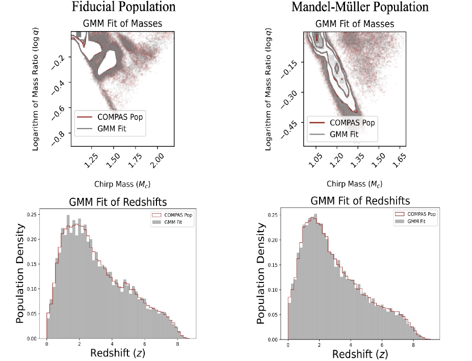
Figure 6: The corner plots and histograms display the marginalized distributions of masses and redshift for both the fiducial and Mandel-Müller populations, along with their GMM fits. Code to generate these plots is available: here.

Firstly, there are fewer formation channels that contribute to the population of BNS mergers. While BBH mergers are anticipated to form through a wide range of channels including dynamical interactions, homogeneous evolution, and classical isolated binary evolution (e.g., Mandel & Farmer, 2022), the formation channels for BNS mergers are much more constrained. Specifically, BNSs are expected to form primarily (if not exclusively) from isolated binary channels involving at least one common envelope event (see e.g., Fig. 1 from Wagg et al. 2022 and, Fig. 6 from Iorio et al. 2023). The reason behind this is that BNS mergers are not expected to form through the ‘stable mass transfer channel’ due to limitations imposed by the critical mass ratio required for this channel (e.g., van Son et al., 2022b; Picco et al., 2024). This implies that we primarily need to focus on the redshift dependence and delay-time distribution of the ‘common envelope channel,’ which is expected to produce relatively short delay times peaking around 1 Gyr (e.g., Fishbach & van Son, 2023), leading to a BNS merger rate that closely tracks the overall star formation rate.

Second, BNS formation (or the yield per unit of star formation) has been shown to be much less sensitive to, or even unaffected by, the formation metallicity. This is in stark contrast to BBH formation, that has repeatedly been shown to drop at high metallicities. This behavior is consistently observed across various population synthesis models with a very broad variation of physics assumptions (including BPASS, MOBSE, StarTrack, COMPAS, SEVN Eldridge & Stanway, 2016; Giacobbo & Mapelli, 2018; Giacobbo et al., 2018; Klencki et al., 2018; Neijssel et al., 2019; Santoliquido et al., 2021; Broekgaarden et al., 2022; Iorio et al., 2023; Fishbach & van Son, 2023). DCO formation through the CE channel is influenced by metallicity-dependent winds, which reduce the progenitor core masses. For BBHs, lower-mass BHs receive larger natal kicks because these kicks are assumed to scale inversely with mass. Hence this leads to a loss of potential BBHs at high metallicities. In contrast, neutron star progenitors are not assumed to experience mass-scaled natal kicks, and thus BNS formation is not sensitive to metallicity in the same way (see van Son et al., in prep for a more in depth discussion of the origin and robustness of this result). This lack of metallicity dependence suggests that the BNS mass distribution will be less impacted by the changing metallicity distribution of star formation across redshifts (Chruślińska, 2024).

Given the single formation channel with a relatively short delay time, and an approximately metallicity-independent yield when marginalized over masses, we expect features in the BNS mass spectrum to be far less dependent on redshift compared to those in the NSBH and BBH mass spectra. As a result, inferring redshift from detector-frame masses under the assumption of a non-evolving mass model becomes less prone to bias.

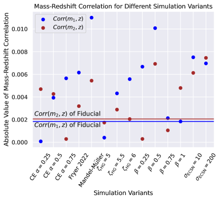
Figure 1: The absolute value of the Pearson correlation coefficient (linear correlation) between mass and redshift for the primary (blue) and secondary (red) neutron star masses across population synthesis variations. Simulation variant names are detailed in the text. The absolute linear correlation remains below 0.02 for all variations. Among these, the Mandel-Müller model shows the highest correlation between primary mass and redshift. Code to generate these plots is available here.

To verify this expectation, we explore variations in uncertain astrophysical parameters that govern BNS mergers, as shown in Figure 1. We focus on physics variations that are expected to have a potentially significant impact on the population of BNS mergers. The population synthesis variations considered are:

1. Common-envelope efficiency, CE $\alpha=0.25,~{}0.5,~{}0.75$.

2. Prescription for the distribution of remnant-masses, and the accompanying natal kick: Fryer et al. (2022), Mandel & Müller (2020).

3. Mass transfer stability parameter for Hertzsprung gap donors, $\zeta_{\text{HG}}=5,~{}5.5,~{}6$ (see Riley et al., 2022, for more details).

4. Mass transfer efficiency; i.e., the fraction of donated mass that is accreted during stable mass transfer $\beta=0.25,~{}0.5,~{}0.75,~{}1$.

5. Width of the Maxwellian distribution of the kick velocity for electron capture supernovae, $\sigma_{\text{ECSN}}=10,~{}200$ (km/s).

As outlined in the COMPAS methods paper (Riley et al., 2022), the fiducial model assumes CE $\alpha$=1, $\zeta_{\text{HG}}=6.5$, and $\sigma_{\text{ECSN}}=30$ (km/s). It adopts the ‘Delayed’ prescriptions from Fryer et al. (2012) for the remnant masses and natal kicks, and has an accretion efficiency $\beta$, that is limited by the thermal timescale of the donor star. To calculate the star formation rate density (SFRD) as a function of redshift and metallicity, we use the cosmic integrator from the COMPAS suite (Neijssel et al., 2019), following the parameters outlined in van Son et al. (2023).

The absolute value of the mass-redshift correlation can increase up to $10$ times compared to the fiducial population (see Figure 1), with the Mandel & Müller (2020) kick prescription. However, this correlation remains below $0.02$ for all variations explored, and including non-linear correlations does not impact the results (see full contour plots here). The low correlation observed between mass and redshift across these models supports our assumption that the mass distribution is nearly independent of redshift.

3 Spectral Siren Cosmology with an Evolving BNS Mass Spectrum

To test whether assuming a redshift-independent BNS mass population biases our cosmological inference, we conduct an injection-recovery campaign by generating mock GW data for BNS mergers. The mock GW data is generated in Cosmic Explorer sensitivity (Evans et al., 2021), with the injected population assumed to be fiducial and Mandel-Müller. We select the Mandel-Müller model because it exhibits the highest mass-redshift correlation (see Fig. 1). If this model still allows for unbiased cosmological parameter inference, then the other models should also be safe.

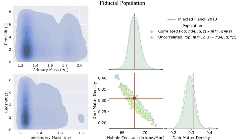
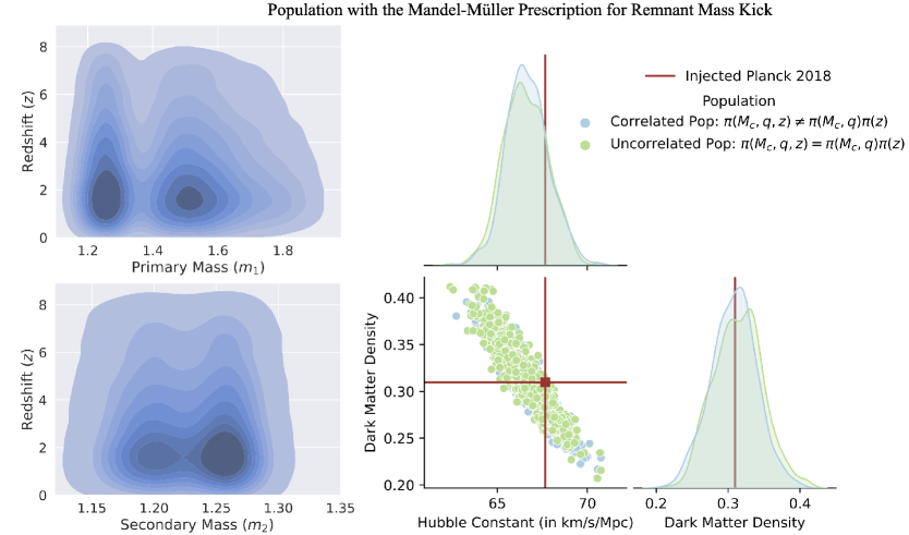
Figure 2: Injection-recovery results for the fiducial model (top) and the Mandel & Müller (2020) remnant-mass and natal kick prescription (bottom). Left: Kernel density estimates of the $m_{1}$ - $z$ and $m_{2}$ - $z$ populations from COMPAS simulations. In both models, peaks and dips remain stationary with redshift, changing only in absolute merger rate based on star formation, suggesting that the BNS mass function is roughly redshift-independent. Right: Inferred matter density and Hubble constant values for both correlated (blue) and uncorrelated (green) populations. Our framework accurately recovers cosmological parameters using both evolving and non-evolving mass models, based on mock data from $800$ binary neutron stars (about 6 days of xG observations at the median BNS merger rate (Abbott et al., 2023b)). For both the fiducial and Mandel & Müller (2020) models, we achieve $\sim 2\%$ constraints on the Hubble constant, which is sufficient to address the Hubble tension. Code to generate these plots is available here and here.

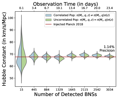
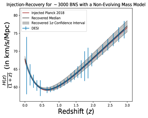
Figure 3: The posterior distribution of the Hubble constant for different numbers of detected BNSs. Left: The evolving (blue) and non-evolving (green) mass models are consistent with each other up to approximately $3,000$ BNS observations, which corresponds to one month of data. We achieve percent-level precision in the Hubble constant within this timeframe when we fix the population. For larger numbers of BNS observations, the width of the posterior does not change significantly, indicating it is suppressed by $1/\sqrt{N}$, where $N$ is the number of BNS observations. Right: The inferred redshift evolution of the Hubble parameter, $H(z)$, divided by $(1+z)$. $H(z)$ is best constrained near $z=0.4$, achieving less than $0.5\%$ error bar. We accurately recover the true curve when we fix the population to the non-evolving mass model. The forecasted error bars from the DESI Collaboration et al. (2016) are also overlaid. Code to generate these plots is available: here.

Our population synthesis simulations provide discrete three-dimensional samples of masses and redshifts. We first fit the population with a three-dimensional Gaussian Mixture Model in chirp mass, mass ratio, and redshift space, and then resample from it. We apply a signal-to-noise ratio (SNR) cut of 8 and adopt the Planck 2018 cosmology (Aghanim et al., 2020) to convert this into the detected population. Additionally, we incorporate parameter estimation (PE) uncertainties from GWs to obtain samples of detector-frame masses and luminosity distances for each BNS binary. See Appendix C for details about the mock data generation.

We validate our cosmological inference framework using the injected fully correlated population of masses and redshift, represented by $\pi(M_{c},q,z)$. Subsequently, we test the assumption of an uncorrelated population, where $\pi(M_{c},q,z)\approx\pi(M_{c},q)\pi(z)$. To model the uncorrelated mass and redshift populations, $\pi(M_{c},q)$ & $\pi(z)$, respectively, we fit them individually using Gaussian Mixture Models with marginalized samples of $M_{c}$, $q$ and $z$ obtained from the injected distribution. Here and throughout our models are assuming that the population distribution is perfectly known. This produces maximally precise cosmological inferences and is therefore more sensitive to biases from unmodeled mass-redshift correlation. A realistic analysis that simultaneously fits the population distribution and cosmology will be even less sensitive to these biases at the cost of additional uncertainty in the cosmological parameters. For further details regarding the inference framework, please refer to Appendix D.

Fig. 2 presents the injection-recovery results for mock data generated under fiducial assumptions and the Mandel-Müller prescription for 800 detected BNS mergers. For both the fiducial and Mandel-Müller data, the joint posterior distributions of the Hubble constant ($H_{0}$) and matter density parameter ($\Omega_{M}$), derived using the assumption of non-evolving mass spectra (uncorrelated case), align with the results obtained when considering the injected population (which may exhibit mass-redshift correlations, i.e., the correlated case). Both methods accurately recover the injected Planck 2018 values with $\sim 2\%$ precision in $H_{0}$, suggesting that a redshift-evolving BNS mass model is not required to address the Hubble tension across all astrophysical variations considered in Section 2.

In Fig. 3, we extend the injection-recovery campaign using fiducial mock data to cover up to one month of observation time with cosmic explorer. No bias is observed when using a non-evolving population model for inference, achieving a $1.14\%$ constraint on $H_{0}$. For $3,000$ BNS mergers in the fiducial universe, the Hubble parameter, $H(z)$, is best constrained at $z=0.4$, with less than $0.5\%$ bias from any redshift evolution in the mass function. This suggests that we can make sub-percent level conclusions about the cosmic history of our universe if it follows the fiducial setup of COMPAS.

Chen et al. (2024) have achieved a percent-level constraint on $H_{0}$ using 50,000 BNS mergers in xG detectors, jointly inferring population and cosmology with a non-evolving uniform mass model. In contrast, by fixing the mass function first to the injected model and then to the non-evolving model, we obtain tighter constraints than Chen et al. (2024). Based on the constraints from Chen et al. (2024), we may expect the lack of bias from a non-evolving mass model to remain valid over a year of observation time if we simultaneously infer population and cosmology. The degree of additional uncertainty from this simultaneous inference also depends on the complexity of the population model. Nonetheless, our study suggests that accurately modeling the true mass population marginalized over redshift will not introduce biases in cosmological parameters across various astrophysically motivated BNS catalogs, even at percent-level precision in the Hubble constant.

4 Conclusion and Future Work

In this paper, we have evaluated BNS populations as spectral sirens, specifically examining the bias introduced by assuming a redshift-uncorrelated population, $\pi(M_{c},q)\pi(z)$, compared to the injected population, $\pi(M_{c},q,z)$. Our analysis shows that using a non-evolving mass model allows us to recover the injected Hubble constant and matter density parameter accurately (see Fig. 2), across a range of realistic population synthesis models, including a fairly extreme example of mass-redshift correlation in the Mandel-Müller kick prescription. Our results indicate that a redshift-evolving mass model is not required to achieve a $2\%$ constraint on the Hubble constant under reasonable physical assumptions about the evolution of the BNS mass function with redshift. This level of precision in $H_{0}$ is sufficient to make a significant contribution toward resolving the Hubble tension. Extending our injection-recovery campaign to one month of Cosmic Explorer data, we have found that a redshift-evolving mass model is not required to achieve sub-percent level precision in the Hubble constant provided BNS mergers in our universe are similar to those of the fiducial setup of COMPAS.

In this study, we have focused on variations of binary physics parameters that are both widely regarded as uncertain, and that we expect could significantly affect the metallicity dependence of the BNS mass distribution. However, our analysis is by no means exhaustive. The BNS mass distribution may still depend on metallicity, and therefore evolve with redshift, if parameters like the neutron star natal kick distribution or common envelope physics vary intrinsically with metallicity. In future work, we plan to explore such variations to determine whether the BNS distribution can be made redshift-dependent. Nonetheless, we anticipate that the BNS mass distribution is far less prone to redshift evolution than the BBH/NSBH mass distribution (see section 2).

We have performed the COMPAS simulation using the median rate provided by the LVK collaboration (Abbott et al., 2023b). However, the BNS rate reported by LVK has a wide uncertainty range, which could affect the accuracy of our mapping from observation time to the number of detections. In the ongoing fourth LVK observing run, no BNS mergers have been detected yet. Although the GWTC-4-informed BNS rate is not publicly available, depending on the actual rate, verifying the existence of Hubble tension with Cosmic Explorer may require more or less than one month of observation time, assuming the population model is fixed.

5 Data Release and Software

The data used in this work is available on Zenodo under an open-source Creative Commons Attribution license at https://zenodo.org/records/14031505 (catalog 10.5281/zenodo.14031505). The corresponding codes are available here: https://github.com/SoumendraRoy/RedevolBNS.

This work made use of the following software packages: COMPAS version v02.46.01 (Stevenson et al., 2017; Vigna-Gómez et al., 2018; Riley et al., 2022), astropy (Astropy Collaboration et al., 2013, 2018, 2022), matplotlib (Hunter, 2007), numpy (Harris et al., 2020), pandas (Wes McKinney, 2010; pandas development team, 2023), python (Van Rossum & Drake, 2009), scipy (Virtanen et al., 2020; Gommers et al., 2023), corner.py (Foreman-Mackey, 2016; Foreman-Mackey et al., 2021), Cython (Behnel et al., 2011), h5py (Collette, 2013; Collette et al., 2023), JAX (Bradbury et al., 2018), numpyro (Phan et al., 2019; Bingham et al., 2019), Jupyter (Perez & Granger, 2007; Kluyver et al., 2016), and seaborn (Waskom, 2021).

Software citation information aggregated using The Software Citation Station (Wagg & Broekgaarden, 2024, 2024).

Appendix A Comparison of Astrophysical Observations with the BNS Population in COMPAS

Although the BNS mass function is roughly redshift-independent in our models, its shape varies significantly depending on binary physics choices and initial conditions (see, for example, Fig. 1 in van Son et al. (in prep) and the primary-secondary mass corner plot for simulation variations in Section 2: link). Here, we compare the mass function for the fiducial COMPAS setup with observed astrophysical neutron star mass measurements. We note that this fiducial population aligns with the galactic binary pulsar population inferred by Farrow et al. (2019) and with binary neutron star merger populations observed in GW events (Abbott et al., 2023b).

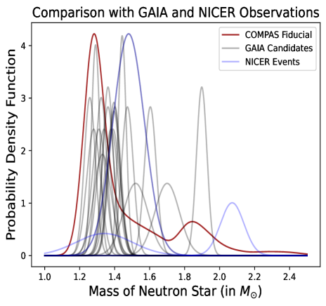
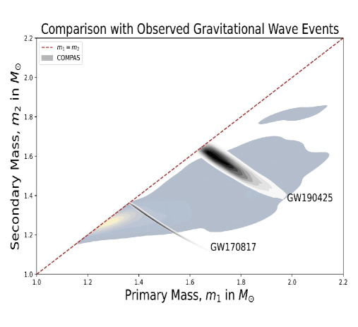
Figure 4: Comparison of individual neutron star mass measurements with the BNS mass population from the fiducial setup in COMPAS. Left: Mass measurements from GAIA and NICER are overlaid on the fiducial mass spectrum. Here y-axis is scaled arbitrarily. Right: Parameter estimation contours for GW170817 and GW190425 are shown against the fiducial population. Code to generate these plots is available: here.

In Fig. 4, we show neutron star mass measurements for $21$ GAIA candidates (El-Badry et al., 2024) and three NICER observations: PSR J0030+0451 (Riley et al., 2019), PSR J0740+6620 (Riley et al., 2021), and PSR J0437–4715 (Choudhury et al., 2024). We also display parameter estimation contours of the two BNS events detected through GWs so far: GW170817 (Abbott et al., 2017) and GW190425 (Abbott et al., 2020), analyzed with the IMRPhenomPv2_NRTidal waveform model and low-spin prior. As shown in Fig. 4, the range of masses covered by these events are broadly consistent with the fiducial BNS mass spectrum in COMPAS.

Appendix B Gaussian Mixture Model Fitting of the True Binary Neutron Star Population

We draw $10^{5}$ samples of source-frame chirp mass ($M_{c}$), logarithm of mass ratio ($\log q$), and redshift ($z$) from COMPAS population using a bounded kernel density estimator with the reflection technique (Gasser & Müller, 1979; Hall & Wehrly, 1991). The bounds are,

$$M_{c}=(-\infty,\infty),~{}\log q=(-\infty,0],~{}z=[0,\infty)$$

While $M_{c}$ should theoretically be bounded between $[0,\infty)$, in practice, no sample falls below $1M_{\odot}$. Therefore, treating $M_{c}$ as unbounded is sufficient.

From these, we first split off $50\%$, of the samples data as the “train” set, and fit GMMs with varying numbers of components with them. Then we evaluate the likelihood of the rest $50\%$ “test” set samples to optimize number of GMM components. We denote the normalized population fitted by the GMM as $f^{\text{GMM}}_{\text{3D}}(M_{c},q,z)$. This $f^{\text{GMM}}_{\text{3D}}(M_{c},q,z)$ is a representation of the true population generated by COMPAS.

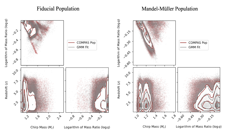
Figure 5: The corner plots show the COMPAS populations of masses and redshifts for both the fiducial setup and the Mandel-Müller kick prescription for remnant mass, along with the GMM fit of these populations. Code to generate these plots is available: here.

Appendix C Mock Data Generation

We summarize the mock data generation process for detector-frame chirp mass ($M_{c}^{\text{det}}$), mass-ratio ($q$), and luminosity distance ($D_{L}$) as follows:

1. COMPAS provides the number of merging BNSs per unit volume per unit merging time for discrete three-dimensional source-frame samples of masses and redshift. By multiplying the number of merging BNSs per unit volume per unit merging time by $4\pi\frac{dV_{c}}{dz}\frac{T_{\text{obs}}}{(1+z)}$, we obtain the expected number of BNS mergers, $N_{\text{exp}}$. Here we assume the Planck 2018 cosmology (Aghanim et al., 2020), with $V_{c}$ and $T_{\text{obs}}$ representing the comoving volume and observation time, respectively. We then perform a Poisson draw with a mean of $N_{\text{exp}}$ to estimate the number of BNS mergers, $N_{\text{obs}}$, that would be observed within the specified observation time, assuming no selection effects,

   $$N_{\text{obs}}\sim\operatorname{Poisson}(N_{\text{exp}})$$

2. Given $N_{\text{obs}}$, we generate the true values of $M_{c}^{t}$, $q^{t}$, and $z^{t}$ by resampling from the true population $f^{\text{GMM}}_{\text{3D}}(M_{c}^{t},q^{t},z^{t})$:

   $$M_{c}^{t},~{}q^{t},~{}z^{t}\sim f^{\text{GMM}}_{\text{3D}}(M_{c}^{t},q^{t},z^{t})$$

   We convert these to the detector-frame values by multiplying $M_{c}^{t}$ by $(1+z^{t})$ and calculating the luminosity distance, $D_{L}^{t}$ for $z^{t}$ using Planck 2018 cosmology:

   $$M^{\text{det},t}_{c}=M_{c}^{t}(1+z),~{}D_{L}^{t}=D_{L}^{t}(z^{t};~{}\text{Planck 2018})$$

   We sample the Finn and Chernoff parameter (Finn & Chernoff, 1993), $\Theta^{t}$, from a $\texttt{Beta}(2,4)$ distribution, which approximates the actual distribution closely:

   $$\Theta^{t}\sim\texttt{Beta}(2,4)$$

3. To obtain PE samples of $M_{c}^{\text{det},t}$, $q^{t}$, and $D_{L}^{t}$ for each BNS observation, we should create a ‘true’ waveform and inject it into the noise of an xG detector. The resulting signal with added noise provides us ‘mock’ GW data, and we perform a full PE analysis on it. Given the computational expense and the lack of fully established techniques for PE in the next-generation multi-detector setup, we resort to an approximate PE approach (Fishbach et al., 2020; Fairhurst et al., 2023; Farah et al., 2023; Essick & Fishbach, 2023).

   We first calculate the true SNR, $\rho^{t}$, using $M^{\text{det},t}_{c}$, $q^{t}$, $\Theta^{t}$, and $D_{L}^{t}$ for each BNS merger:

   $$\rho^{t}=\Bigg{[}4\int_{0}^{\infty}df\frac{|h(M^{\text{det},t}_{c},q^{t},\Theta^{t},D_{L}^{t};f)|^{2}}{S_{n}(f)}\Bigg{]}^{\frac{1}{2}}$$ (C1)

   Here, $h(M^{\text{det},t}_{c},q^{t},\Theta^{t},D_{L}^{t};f)$ is the waveform model, and $S_{n}(f)$ is the power spectral density of Cosmic Explorer with a $40$ km baseline (Srivastava et al., 2022). We use the single-spin precessing waveform model IMRPhenomPv2 (Husa et al., 2016; Khan et al., 2016) with all individual spin components set to zero. Evaluating the integral in equation (C1) is computationally intensive, especially across the parameter space of BNSs. Therefore, we pre-compute the integral for a two-dimensional grid of face-on masses at a reference distance $D_{L}^{t}=1$ Gpc and interpolate for the desired masses. We then find $\rho^{t}$ at our required Finn and Chernoff parameter and luminosity distance by scaling:

   $$\rho^{t}(M^{\text{det},t}_{c},q^{t},\Theta^{t},D_{L}^{t})=\frac{\Theta^{t}}{D_{L}^{t}}\times\rho^{t}(M^{\text{det},t}_{c},q^{t},\Theta^{t}=1,D_{L}^{t}=1~{}\text{Gpc})$$

   We determine the observed SNR, $\rho_{\text{obs}}$, by adding Gaussian noise with a standard deviation of $1$ to $\rho^{t}$:

   $$\rho^{\text{obs}}\sim\operatorname{N}(\rho^{t},1)$$ (C2)

   Finally, we apply a selection cut by retaining only BNS mergers with $\rho^{\text{obs}}>8$.

4. For BNS mergers above the selection threshold, we aim to create and sample from the joint posterior distribution of the parameters: detector-frame chirp mass, logarithm of mass ratio, Finn and Chernoff parameter, and luminosity distance. The posterior distribution is given by:

   $$P(M^{\text{det}}_{c},\log q,\Theta,D_{L}|M^{\text{det},\text{obs}}_{c},\log q^{\text{obs}},\Theta^{\text{obs}},D^{L,\text{obs}})\propto\Big{|}\frac{\partial\rho}{\partial D_{L}}\Big{|}\times\pi(M^{\text{det}}_{c},\log q,\Theta,\rho)\times$$

   $$\mathcal{L}(M^{\text{det},\text{obs}}_{c},\log q^{\text{obs}},\Theta^{\text{obs}},\rho^{\text{obs}}|M^{\text{det}}_{c},\log q,\Theta,\rho)$$ (C3)

   where $\pi(M^{\text{det}}_{c},\log q,\Theta,\rho)$ represents the joint prior over the parameters, and $M^{\text{det},\text{obs}}_{c},\log q^{\text{obs}},\Theta^{\text{obs}},\rho^{\text{obs}}$ are the observed values of these parameters.

   To draw samples of $M^{\text{det}}_{c}$, $\log q$, $\Theta$, and $D_{L}$ from Equation (C3), we proceed as follows:

   1. Calculate Observed PE Uncertainty: We determine the PE uncertainties by scaling the benchmark values from Vitale & Evans (2017) according to the observed SNR ($\rho^{\text{obs}}$). We denote the error bars on $M^{\text{det}}_{c},\log q,$ and $\Theta$ as $\sigma_{M^{\text{det}}_{c}},\sigma_{\log q},$ and $\sigma_{\Theta}$, respectively.

   2. Draw Observed Quantities: For each event, draw one sample of the observed quantities:

      $$M^{\text{det},\text{obs}}_{c}\sim\operatorname{N}(M^{\text{det}}_{c},\sigma_{M^{\text{det}}_{c}}),~{}\log q^{\text{obs}}\sim\operatorname{N}_{(-\infty,0]}(\log q,\sigma_{\log q}),~{}\Theta^{\text{obs}}\sim\operatorname{N}_{[0,0.25]}(\Theta,\sigma_{\Theta})$$ (C4)

      where for $\operatorname{N}_{[a,b]}(\mu,\sigma)$ is a truncated normal distribution with mean $\mu$ and standard deviation $\sigma$ within the bounds $[a,b]$.

      One notable difference between our mock data generation process and that of Fishbach et al. (2020) is that while Fishbach et al. (2020) assumed $M^{\text{det}}_{c}$ follows a lognormal distribution to avoid negative values of $M^{\text{det},\text{obs}}_{c}$, we verified that for our values of $\sigma_{M^{\text{det}}_{c}}$, $M^{\text{det},\text{obs}}_{c}$ is never negative.

   3. Generate Multiple Samples: For each observed event, generate $N_{\text{samp}}$ samples (ranging from 1000 to 8000, depending on the number of events):

      $$M^{\text{det}}_{c}\sim\operatorname{N}(M^{\text{det},\text{obs}}_{c},\sigma_{M^{\text{det}}_{c}}),~{}\log q\sim\frac{\operatorname{N}_{(-\infty,0]}(\log q^{\text{obs}},\sigma_{\log q})}{\Phi\big{(}\frac{-\log q}{\sigma_{\log q}}\big{)}},~{}\Theta\sim\frac{\operatorname{N}_{[0,0.25]}(\Theta^{\text{obs}},\sigma_{\Theta})}{\Big{[}\Phi\big{(}\frac{0.25-\Theta}{\sigma_{\Theta}}\big{)}-\Phi\big{(}-\frac{\Theta}{\sigma_{\Theta}}\big{)}\Big{]}},~{}\rho\sim\operatorname{N}(\rho^{\text{obs}},1)$$ (C5)

      $\Phi(.)$ represents the cumulative distribution for normal distribution.

   4. Calculate Luminosity Distance: Using the samples of $M^{\text{det}}_{c},\log q,\Theta$, and $\rho$ from (C5), determine $D_{L}$ for each event as:

      $$D_{L}=\frac{\Theta}{\rho}\times\rho^{t}(M^{\text{det}}_{c},\log q,\Theta=1,D^{\text{fid}}_{L}=1\text{Gpc})$$ (C6)

   5. Reweight Samples: Reweight the samples by:

      $$w=\Big{|}\frac{\partial\rho}{\partial D_{L}}\Big{|}=\frac{\rho}{D_{L}}$$ (C7)

   Finally, for each of the $N_{obs}$ BNS mergers, we obtain $N_{\text{samp}}$ samples of $M^{\text{det}}_{c}$, $\log q$, $\Theta$, and $D_{L}$ which together represent the posterior distribution of PE using a uniform PE prior.

Appendix D Method

In Appendices B and C, we discussed generating mock data to represent PE samples in Cosmic Explorer for different true population distributions. Next, we estimate the cosmological parameters, $\vec{\Omega}_{C}$, using these datasets. To achieve this, we deconvolve the error bars induced by PE (Bovy et al., 2011). This process yields the rate-marginalized posterior distribution of $\vec{\Omega}_{C}$, incorporating a hierarchical prior proportional to the inverse of the rate (Essick & Farr, 2022).

The posterior distribution of $\vec{\Omega}_{C}$ is approximately given by (Loredo, 2004; Mandel et al., 2019):

$$\text{Posterior of}~{}\vec{\Omega}_{C}~{}~{}~{}~{}\stackrel{{\scriptstyle\mathclap{\mbox{approx}}}}{{\propto}}~{}~{}~{}~{}\pi(\vec{\Omega}_{C})\xi^{-N_{\text{\text{obs}}}}\prod\limits_{i}^{N_{\text{\text{obs}}}}\sum\limits_{M_{c}^{\text{det},i},q^{i},D_{L}^{i}}\frac{1}{\pi_{\text{PE}}(M_{c}^{\text{det}},q,D_{L})}.\frac{\frac{dz}{dD_{L}}}{1+z}.\pi(M_{c},q,z)\Bigg{|}_{M_{c}=\frac{M_{c}^{\text{det}}}{1+z(D_{L},\vec{\Omega}_{C})},~{}z=z(D_{L},\vec{\Omega}_{C})}$$ (D1)

Here, $\pi(\vec{\Omega}_{C})$ represents the hierarchical prior for $\vec{\Omega}_{C}$ and $\xi$ is the selection function corresponding to the SNR cut of $8$ in Cosmic Explorer noise. $M_{c}^{\text{det},i}$, $q^{i}$, and $D_{L}^{i}$ are the samples from the $i$-th event’s PE posterior. We also fully marginalize over the Finn and Chernoff parameter, $\Theta$ since its population is independent of masses and redshift and fixed by isotropy.

We calculate the selection function, $\xi$, by generating injections in the detector frame and performing a Monte Carlo summation in the detector frame (Tiwari, 2018; Farr, 2019),

$$\xi~{}(\vec{\Omega}_{C})\approx\frac{1}{N_{\text{draw}}}\sum\limits_{M_{c}^{\text{det},\text{inj}},q^{\text{inj}},D_{L}^{\text{inj}}}\frac{1}{p_{\text{draw}}(M_{c}^{\text{det}},q,D_{L})}.\frac{\frac{dz}{dD_{L}}}{1+z}.\pi(M_{c},q,z)\Bigg{|}_{M_{c}=\frac{M_{c}^{\text{det}}}{1+z(D_{L},\vec{\Omega}_{C})},~{}z=z(D_{L},\vec{\Omega}_{C})}$$ (D2)

Here, $p_{\text{draw}}$ is the distribution from which the injections are sampled, and $M_{c}^{\text{det},\text{inj}},q^{\text{inj}},D_{L}^{\text{inj}}$ are the injections that meet the detection threshold of the SNR cut of $8$. In Equations (D1) and (D2), $dz/dD_{L}$ and $1/(1+z)$ are Jacobians to convert the population density in the source frame into a density over the samples in the detector frame. We also ensure that the effective number of samples is greater than four times the number of observed BNS mergers (Farr, 2019; Essick & Farr, 2022).

For the correlated case, we use the injected population $f^{\text{GMM}}_{\text{3D}}(M_{c},q,z)$ as described in Appendix B:

$$\pi_{\text{corr}}(M_{c},q,z)=\pi_{\text{inj}}(M_{c},q,z)=f^{\text{GMM}}_{\text{3D}}(M_{c},q,z)$$ (D3)

where $\pi_{\text{corr}}(M_{c},q,z)$ and $\pi_{\text{inj}}(M_{c},q,z)$ represent the correlated and injected populations, respectively.

For the uncorrelated case, we model the mass population, marginalized over redshift, using a two-dimensional Gaussian Mixture Model, $f^{\text{GMM}}_{\text{2D}}(M_{c},q)$, and the redshift population, marginalized over masses, using a one-dimensional Gaussian Mixture Model, $f^{\text{GMM}}_{\text{1D}}(z)$. The uncorrelated population is then given by:

$$\pi_{\text{uncorr}}(M_{c},q,z)=\Big{(}\int_{\forall z}dz~{}\pi_{\text{inj}}(M_{c},q,z)\Big{)}\Big{(}\int_{\forall M_{c},q}dM_{c}~{}dq~{}\pi_{\text{inj}}(M_{c},q,z)\Big{)}=f^{\text{GMM}}_{\text{2D}}(M_{c},q)f^{\text{GMM}}_{\text{1D}}(z)$$ (D4)

Here, $\pi_{\text{uncorr}}(M_{c},q,z)$ represents the uncorrelated mass-redshift population. The population drops to zero beyond mass ratio $1$ and below redshift $0$. The GMM underpredicts the probability density near these hard cutoffs. To compensate for this, we use the reflection technique (Gasser & Müller, 1979; Hall & Wehrly, 1991).

To model the distance ($D_{L}$)–redshift ($z$) relationship, we adopt a flat $\Lambda$CDM cosmology with a radiation density parameter set to zero:

$$D_{L}=\frac{c}{H_{0}}(1+z)\int_{0}^{z}dz^{\prime}\frac{1}{\sqrt{\Omega_{M}(1+z^{\prime})^{3}+(1-\Omega_{M})}}$$ (D5)

We assume uniform priors for the dimensionless Hubble constant ($H_{0}/100~{}\text{km s}^{-1}\text{Mpc}^{-1}$), ranging from $0.2$ to $1.5$, and for the matter density parameter ($\Omega_{M}$), ranging from $0$ to $1$. These priors are applied to both evolving and non-evolving mass models. We use the No-U-Turn Sampler (NUTS) in combination with NumPyro (Phan et al., 2019; Bingham et al., 2019) and JAX (Bradbury et al., 2018) for sampling the cosmological parameters. JAX enables compatibility with automatic differentiation, facilitating efficient sampling.

References

- Abbott et al. (2017) Abbott, B., Abbott, R., Abbott, T., et al. 2017, Physical Review Letters, 119, doi: 10.1103/physrevlett.119.161101
- Abbott et al. (2020) Abbott, B. P., Abbott, R., Abbott, T. D., et al. 2020, The Astrophysical Journal Letters, 892, L3, doi: 10.3847/2041-8213/ab75f5
- Abbott et al. (2023a) Abbott, R., Abe, H., Acernese, F., et al. 2023a, The Astrophysical Journal, 949, 76, doi: 10.3847/1538-4357/ac74bb
- Abbott et al. (2023b) Abbott, R., Abbott, T. D., Acernese, F., et al. 2023b, Phys. Rev. X, 13, 011048, doi: 10.1103/PhysRevX.13.011048
- Acernese et al. (2015) Acernese, F., Agathos, M., Agatsuma, K., et al. 2015, Classical and Quantum Gravity, 32, 024001, doi: 10.1088/0264-9381/32/2/024001
- Aghanim et al. (2020) Aghanim, N., Akrami, Y., Ashdown, M., et al. 2020, Astronomy & Astrophysics, 641, A6, doi: 10.1051/0004-6361/201833910
- Akutsu et al. (2020) Akutsu, T., Ando, M., Arai, K., et al. 2020, Progress of Theoretical and Experimental Physics, 2021, 05A101, doi: 10.1093/ptep/ptaa125
- Astropy Collaboration et al. (2013) Astropy Collaboration, Robitaille, T. P., Tollerud, E. J., et al. 2013, A&A, 558, A33, doi: 10.1051/0004-6361/201322068
- Astropy Collaboration et al. (2018) Astropy Collaboration, Price-Whelan, A. M., Sipőcz, B. M., et al. 2018, AJ, 156, 123, doi: 10.3847/1538-3881/aabc4f
- Astropy Collaboration et al. (2022) Astropy Collaboration, Price-Whelan, A. M., Lim, P. L., et al. 2022, ApJ, 935, 167, doi: 10.3847/1538-4357/ac7c74
- Behnel et al. (2011) Behnel, S., Bradshaw, R., Citro, C., et al. 2011, Computing in Science Engineering, 13, 31, doi: 10.1109/MCSE.2010.118
- Bingham et al. (2019) Bingham, E., Chen, J. P., Jankowiak, M., et al. 2019, J. Mach. Learn. Res., 20, 28:1. http://jmlr.org/papers/v20/18-403.html
- Bovy et al. (2011) Bovy, J., Hogg, D. W., & Roweis, S. T. 2011, The Annals of Applied Statistics, 5, doi: 10.1214/10-aoas439
- Bradbury et al. (2018) Bradbury, J., Frostig, R., Hawkins, P., et al. 2018, JAX: composable transformations of Python+NumPy programs, 0.3.13. http://github.com/google/jax
- Broekgaarden et al. (2024) Broekgaarden, F. S., Banagiri, S., & Payne, E. 2024, ApJ, 969, 108, doi: 10.3847/1538-4357/ad4709
- Broekgaarden et al. (2019) Broekgaarden, F. S., Justham, S., de Mink, S. E., et al. 2019, MNRAS, 490, 5228, doi: 10.1093/mnras/stz2558
- Broekgaarden et al. (2022) Broekgaarden, F. S., Berger, E., Stevenson, S., et al. 2022, MNRAS, 516, 5737, doi: 10.1093/mnras/stac1677
- Chattopadhyay et al. (2020) Chattopadhyay, D., Stevenson, S., Hurley, J. R., Rossi, L. J., & Flynn, C. 2020, Monthly Notices of the Royal Astronomical Society, 494, 1587–1610, doi: 10.1093/mnras/staa756
- Chen et al. (2024) Chen, H.-Y., Ezquiaga, J. M., & Gupta, I. 2024, Cosmography with next-generation gravitational wave detectors. https://arxiv.org/abs/2402.03120
- Chernoff & Finn (1993) Chernoff, D. F., & Finn, L. S. 1993, The Astrophysical Journal, 411, L5, doi: 10.1086/186898
- Choudhury et al. (2024) Choudhury, D., Salmi, T., Vinciguerra, S., et al. 2024, The Astrophysical Journal Letters, 971, L20, doi: 10.3847/2041-8213/ad5a6f
- Chruślińska (2024) Chruślińska, M. 2024, Annalen der Physik, 536, 2200170, doi: 10.1002/andp.202200170
- Collaboration et al. (2016) Collaboration, D., Aghamousa, A., Aguilar, J., et al. 2016, The DESI Experiment Part I: Science,Targeting, and Survey Design. https://arxiv.org/abs/1611.00036
- Collette (2013) Collette, A. 2013, Python and HDF5 (O’Reilly)
- Collette et al. (2023) Collette, A., Kluyver, T., Caswell, T. A., et al. 2023, h5py/h5py: 3.8.0, 3.8.0, Zenodo, doi: 10.5281/zenodo.7560547
- El-Badry et al. (2024) El-Badry, K., Rix, H.-W., Latham, D. W., et al. 2024, The Open Journal of Astrophysics, 7, doi: 10.33232/001c.121261
- Eldridge & Stanway (2016) Eldridge, J. J., & Stanway, E. R. 2016, MNRAS, 462, 3302, doi: 10.1093/mnras/stw1772
- Essick & Farr (2022) Essick, R., & Farr, W. 2022, Precision Requirements for Monte Carlo Sums within Hierarchical Bayesian Inference. https://arxiv.org/abs/2204.00461
- Essick & Fishbach (2023) Essick, R., & Fishbach, M. 2023, DAGnabbit! Ensuring Consistency between Noise and Detection in Hierarchical Bayesian Inference. https://arxiv.org/abs/2310.02017
- Evans et al. (2021) Evans, M., Adhikari, R. X., Afle, C., et al. 2021, A Horizon Study for Cosmic Explorer: Science, Observatories, and Community. https://arxiv.org/abs/2109.09882
- Ezquiaga & Holz (2022) Ezquiaga, J. M., & Holz, D. E. 2022, Physical Review Letters, 129, doi: 10.1103/physrevlett.129.061102
- Fairhurst et al. (2023) Fairhurst, S., Hoy, C., Green, R., Mills, C., & Usman, S. A. 2023, Phys. Rev. D, 108, 082006, doi: 10.1103/PhysRevD.108.082006
- Farah et al. (2023) Farah, A. M., Edelman, B., Zevin, M., et al. 2023, The Astrophysical Journal, 955, 107, doi: 10.3847/1538-4357/aced02
- Farr (2019) Farr, W. M. 2019, Research Notes of the AAS, 3, 66, doi: 10.3847/2515-5172/ab1d5f
- Farr et al. (2019) Farr, W. M., Fishbach, M., Ye, J., & Holz, D. E. 2019, The Astrophysical Journal Letters, 883, L42, doi: 10.3847/2041-8213/ab4284
- Farrow et al. (2019) Farrow, N., Zhu, X.-J., & Thrane, E. 2019, The Astrophysical Journal, 876, 18, doi: 10.3847/1538-4357/ab12e3
- Finn & Chernoff (1993) Finn, L. S., & Chernoff, D. F. 1993, Phys. Rev. D, 47, 2198, doi: 10.1103/PhysRevD.47.2198
- Fishbach et al. (2020) Fishbach, M., Farr, W. M., & Holz, D. E. 2020, The Astrophysical Journal Letters, 891, L31, doi: 10.3847/2041-8213/ab77c9
- Fishbach & van Son (2023) Fishbach, M., & van Son, L. 2023, The Astrophysical Journal Letters, 957, L31, doi: 10.3847/2041-8213/ad0560
- Foreman-Mackey (2016) Foreman-Mackey, D. 2016, The Journal of Open Source Software, 1, 24, doi: 10.21105/joss.00024
- Foreman-Mackey et al. (2021) Foreman-Mackey, D., Price-Whelan, A., Vousden, W., et al. 2021, dfm/corner.py: corner.py v.2.2.1, v2.2.1, Zenodo, doi: 10.5281/zenodo.4592454
- Fryer et al. (2012) Fryer, C. L., Belczynski, K., Wiktorowicz, G., et al. 2012, The Astrophysical Journal, 749, 91, doi: 10.1088/0004-637X/749/1/91
- Fryer et al. (2022) Fryer, C. L., Olejak, A., & Belczynski, K. 2022, The Astrophysical Journal, 931, 94, doi: 10.3847/1538-4357/ac6ac9
- Gasser & Müller (1979) Gasser, T., & Müller, H.-G. 1979, in Smoothing Techniques for Curve Estimation, ed. T. Gasser & M. Rosenblatt (Berlin, Heidelberg: Springer Berlin Heidelberg), 23–68
- Giacobbo & Mapelli (2018) Giacobbo, N., & Mapelli, M. 2018, MNRAS, 480, 2011, doi: 10.1093/mnras/sty1999
- Giacobbo et al. (2018) Giacobbo, N., Mapelli, M., & Spera, M. 2018, MNRAS, 474, 2959, doi: 10.1093/mnras/stx2933
- Gommers et al. (2023) Gommers, R., Virtanen, P., Burovski, E., et al. 2023, scipy/scipy: SciPy 1.11.0, v1.11.0, Zenodo, doi: 10.5281/zenodo.8079889
- Hall & Wehrly (1991) Hall, P., & Wehrly, T. E. 1991, Journal of the American Statistical Association, 86, 665, doi: 10.1080/01621459.1991.10475092
- Harris et al. (2020) Harris, C. R., Millman, K. J., van der Walt, S. J., et al. 2020, Nature, 585, 357, doi: 10.1038/s41586-020-2649-2
- Holz & Hughes (2005) Holz, D. E., & Hughes, S. A. 2005, ApJ, 629, 15, doi: 10.1086/431341
- Hunter (2007) Hunter, J. D. 2007, Computing in Science & Engineering, 9, 90, doi: 10.1109/MCSE.2007.55
- Husa et al. (2016) Husa, S., Khan, S., Hannam, M., et al. 2016, Phys. Rev. D, 93, 044006, doi: 10.1103/PhysRevD.93.044006
- Iorio et al. (2023) Iorio, G., Mapelli, M., Costa, G., et al. 2023, Monthly Notices of the Royal Astronomical Society, 524, 426–470, doi: 10.1093/mnras/stad1630
- Karathanasis et al. (2023) Karathanasis, C., Mukherjee, S., & Mastrogiovanni, S. 2023, Monthly Notices of the Royal Astronomical Society, 523, 4539–4555, doi: 10.1093/mnras/stad1373
- Khan et al. (2016) Khan, S., Husa, S., Hannam, M., et al. 2016, Phys. Rev. D, 93, 044007, doi: 10.1103/PhysRevD.93.044007
- Klencki et al. (2018) Klencki, J., Moe, M., Gladysz, W., et al. 2018, A&A, 619, A77, doi: 10.1051/0004-6361/201833025
- Kluyver et al. (2016) Kluyver, T., Ragan-Kelley, B., Pérez, F., et al. 2016, in ELPUB, 87–90
- Loredo (2004) Loredo, T. J. 2004, in AIP Conference Proceedings (AIP), doi: 10.1063/1.1835214
- Mandel & Farmer (2022) Mandel, I., & Farmer, A. 2022, Phys. Rep., 955, 1, doi: 10.1016/j.physrep.2022.01.003
- Mandel et al. (2019) Mandel, I., Farr, W. M., & Gair, J. R. 2019, Monthly Notices of the Royal Astronomical Society, 486, 1086, doi: 10.1093/mnras/stz896
- Mandel & Müller (2020) Mandel, I., & Müller, B. 2020, Monthly Notices of the Royal Astronomical Society, 499, 3214–3221, doi: 10.1093/mnras/staa3043
- Mapelli et al. (2022) Mapelli, M., Bouffanais, Y., Santoliquido, F., Arca Sedda, M., & Artale, M. C. 2022, MNRAS, 511, 5797, doi: 10.1093/mnras/stac422
- Mapelli et al. (2019) Mapelli, M., Giacobbo, N., Santoliquido, F., & Artale, M. C. 2019, MNRAS, 487, 2, doi: 10.1093/mnras/stz1150
- Mastrogiovanni et al. (2021) Mastrogiovanni, S., Leyde, K., Karathanasis, C., et al. 2021, Phys. Rev. D, 104, 062009, doi: 10.1103/PhysRevD.104.062009
- Messenger & Read (2012) Messenger, C., & Read, J. 2012, Physical Review Letters, 108, doi: 10.1103/physrevlett.108.091101
- Mukherjee (2022) Mukherjee, S. 2022, Monthly Notices of the Royal Astronomical Society, 515, 5495–5505, doi: 10.1093/mnras/stac2152
- Neijssel et al. (2019) Neijssel, C. J., Vigna-Gómez, A., Stevenson, S., et al. 2019, MNRAS, 490, 3740, doi: 10.1093/mnras/stz2840
- pandas development team (2023) pandas development team, T. 2023, pandas-dev/pandas: Pandas, v2.1.2, Zenodo, doi: 10.5281/zenodo.10045529
- Perez & Granger (2007) Perez, F., & Granger, B. E. 2007, Computing in Science and Engineering, 9, 21, doi: 10.1109/MCSE.2007.53
- Phan et al. (2019) Phan, D., Pradhan, N., & Jankowiak, M. 2019, arXiv e-prints, arXiv:1912.11554, doi: 10.48550/arXiv.1912.11554
- Picco et al. (2024) Picco, A., Marchant, P., Sana, H., & Nelemans, G. 2024, A&A, 681, A31, doi: 10.1051/0004-6361/202347090
- Pierra et al. (2023) Pierra, G., Mastrogiovanni, S., Perriès, S., & Mapelli, M. 2023, A Study of Systematics on the Cosmological Inference of the Hubble Constant from Gravitational Wave Standard Sirens. https://arxiv.org/abs/2312.11627
- Riess et al. (2022) Riess, A. G., Yuan, W., Macri, L. M., et al. 2022, The Astrophysical Journal Letters, 934, L7, doi: 10.3847/2041-8213/ac5c5b
- Riley et al. (2022) Riley, J., Agrawal, P., Barrett, J. W., et al. 2022, The Astrophysical Journal Supplement Series, 258, 34, doi: 10.3847/1538-4365/ac416c
- Riley et al. (2022) Riley, J., Agrawal, P., Barrett, J. W., et al. 2022, ApJS, 258, 34, doi: 10.3847/1538-4365/ac416c
- Riley et al. (2019) Riley, T. E., Watts, A. L., Bogdanov, S., et al. 2019, The Astrophysical Journal Letters, 887, L21, doi: 10.3847/2041-8213/ab481c
- Riley et al. (2021) Riley, T. E., Watts, A. L., Ray, P. S., et al. 2021, The Astrophysical Journal Letters, 918, L27, doi: 10.3847/2041-8213/ac0a81
- Santoliquido et al. (2021) Santoliquido, F., Mapelli, M., Giacobbo, N., Bouffanais, Y., & Artale, M. C. 2021, MNRAS, 502, 4877, doi: 10.1093/mnras/stab280
- Schutz (1986) Schutz, B. F. 1986, Nature, 323, 310, doi: 10.1038/323310a0
- Srivastava et al. (2022) Srivastava, V., Davis, D., Kuns, K., et al. 2022, The Astrophysical Journal, 931, 22, doi: 10.3847/1538-4357/ac5f04
- Stevenson et al. (2017) Stevenson, S., Vigna-Gómez, A., Mandel, I., et al. 2017, Nature Communications, 8, 14906, doi: 10.1038/ncomms14906
- Taylor & Gair (2012) Taylor, S. R., & Gair, J. R. 2012, Physical Review D, 86, doi: 10.1103/physrevd.86.023502
- Taylor et al. (2012) Taylor, S. R., Gair, J. R., & Mandel, I. 2012, Physical Review D, 85, doi: 10.1103/physrevd.85.023535
- The LIGO Scientific Collaboration et al. (2015) The LIGO Scientific Collaboration, Aasi, J., Abbott, B. P., et al. 2015, Classical and Quantum Gravity, 32, 074001, doi: 10.1088/0264-9381/32/7/074001
- Tiwari (2018) Tiwari, V. 2018, Classical and Quantum Gravity, 35, 145009, doi: 10.1088/1361-6382/aac89d
- Van Rossum & Drake (2009) Van Rossum, G., & Drake, F. L. 2009, Python 3 Reference Manual (Scotts Valley, CA: CreateSpace)
- van Son et al. (2023) van Son, L. A. C., de Mink, S. E., Chruślińska, M., et al. 2023, ApJ, 948, 105, doi: 10.3847/1538-4357/acbf51
- van Son et al. (2022a) van Son, L. A. C., de Mink, S. E., Callister, T., et al. 2022a, The Astrophysical Journal, 931, 17, doi: 10.3847/1538-4357/ac64a3
- van Son et al. (2022b) van Son, L. A. C., de Mink, S. E., Renzo, M., et al. 2022b, The Astrophysical Journal, 940, 184, doi: 10.3847/1538-4357/ac9b0a
- Vigna-Gómez et al. (2018) Vigna-Gómez, A., Neijssel, C. J., Stevenson, S., et al. 2018, Monthly Notices of the Royal Astronomical Society, 481, 4009, doi: 10.1093/mnras/sty2463
- Virtanen et al. (2020) Virtanen, P., Gommers, R., Oliphant, T. E., et al. 2020, Nature Methods, 17, 261, doi: 10.1038/s41592-019-0686-2
- Vitale & Evans (2017) Vitale, S., & Evans, M. 2017, Phys. Rev. D, 95, 064052, doi: 10.1103/PhysRevD.95.064052
- Wagg & Broekgaarden (2024) Wagg, T., & Broekgaarden, F. 2024, The Software Citation Station, Zenodo, doi: 10.5281/zenodo.11292917
- Wagg & Broekgaarden (2024) Wagg, T., & Broekgaarden, F. S. 2024, arXiv e-prints, arXiv:2406.04405. https://arxiv.org/abs/2406.04405
- Wagg et al. (2022) Wagg, T., Broekgaarden, F. S., de Mink, S. E., et al. 2022, The Astrophysical Journal, 937, 118, doi: 10.3847/1538-4357/ac8675
- Waskom (2021) Waskom, M. L. 2021, Journal of Open Source Software, 6, 3021, doi: 10.21105/joss.03021
- Wes McKinney (2010) Wes McKinney. 2010, in Proceedings of the 9th Python in Science Conference, ed. Stéfan van der Walt & Jarrod Millman, 56 – 61, doi: 10.25080/Majora-92bf1922-00a
- Ye & Fishbach (2024) Ye, C. S., & Fishbach, M. 2024, ApJ, 967, 62, doi: 10.3847/1538-4357/ad3ba8
- Zhu et al. (2018) Zhu, X., Thrane, E., Osłowski, S., Levin, Y., & Lasky, P. D. 2018, Phys. Rev. D, 98, 043002, doi: 10.1103/PhysRevD.98.043002
- Zhu & Ashton (2020) Zhu, X.-J., & Ashton, G. 2020, The Astrophysical Journal Letters, 902, L12, doi: 10.3847/2041-8213/abb6ea