Benchmarking XAI Explanations with Human-Aligned Evaluations

Abstract

In this paper, we introduce PASTA (Perceptual Assessment System for explanaTion of Artificial intelligence), a novel framework for a human-centric evaluation of XAI techniques in computer vision. Our first key contribution is a human evaluation of XAI explanations on four diverse datasets—COCO, Pascal Parts, Cats Dogs Cars, and MonumAI—which constitutes the first large-scale benchmark dataset for XAI, with annotations at both the image and concept levels. This dataset allows for robust evaluation and comparison across various XAI methods. Our second major contribution is a data-based metric for assessing the interpretability of explanations. It mimics human preferences, based on a database of human evaluations of explanations in the PASTA-dataset. With its dataset and metric, the PASTA framework provides consistent and reliable comparisons between XAI techniques, in a way that is scalable but still aligned with human evaluations. Additionally, our benchmark allows for comparisons between explanations across different modalities, an aspect previously unaddressed. Our findings indicate that humans tend to prefer saliency maps over other explanation types. Moreover, we provide evidence that human assessments show a low correlation with existing XAI metrics that are numerically simulated by probing the model.

1 Introduction

As Deep Neural Networks (DNNs) systems are being used in increasingly high stakes domains (e.g., legal, medical) (Surden, 2021; Litjens et al., 2017), it is essential that humans are able to interpret how they reach their conclusions. (Bender et al., 2021). Their lack of transparency has led them to be characterized as “black boxes” (Castelvecchi, 2016), which is particularly problematic in critical applications where understanding the decision-making process is essential for trust and accountability (Vereschak et al., 2024), leading to the creation of a relatively new field: explainable AI (XAI) (Gunning et al., 2019). XAI aims to make the workings of deep learning models more transparent and interpretable. XAI methods fall into two main categories: post-hoc techniques (Selvaraju et al., 2017; Ribeiro et al., 2016; Lundberg & Lee, 2017) and ante-hoc techniques (Bennetot et al., 2022; Koh et al., 2020). Post-hoc techniques generally explain the output of a frozen, pretrained DNN, while ante-hoc techniques modify the architecture of the DNN to improve its interpretability from the outset. Each of these categories can be further subdivided into various sub-families, offering a wide array of XAI approaches.

The diversity of XAI techniques calls for an effort to standardize their evaluation and comparison. Although there are toolkits in computer vision that offer a range of computational evaluation techniques (Hedström et al., 2023; Fel et al., 2022a), to our knowledge there has been no effort to standardize their evaluation from a perceptual point of view (Nauta et al., 2023), i.e., the way the explanation is perceived by the human for whom it was intended. Currently, prevalent approaches (Dawoud et al., 2023; Colin et al., 2022) to evaluating XAI techniques involve human annotators assessing and ranking their interpretability. This approach aligns with XAI’s goal of improving the human interpretability of DNN models. Yet, this method is costly since it requires paying annotators and is impractical for widespread use, as each new XAI technique necessitates a fresh round of human evaluation. It is also at risk of being inconsistent and unreliable since evaluations may differ from one annotator to another and depend on factors such as fatigue and even the time of day (Schmidt et al., 2007).

To address the challenges associated with evaluating XAI techniques, we propose the Perceptual Assessment System for explanaTion of Artificial intelligence (PASTA). PASTA aims to automate the evaluation of XAI techniques by providing an evaluation metric that mimics human assessments.

The first component of PASTA is a dataset composed of four diverse datasets (COCO, Pascal Part, Cats Dogs Cars, and Monumai), which includes both image and concept annotations. Using this dataset, we compare 21 XAI methods across multiple model architectures. We subject the resulting explanations to a rigorous evaluation by human annotators, along a comprehensive set of criteria that cover a variety of desired properties.

The second component of PASTA is a metric designed to replicate human evaluation on the PASTA-dataset. While there are benchmarks that focus on perceptual evaluation of XAI methods (Colin et al., 2022; Dawoud et al., 2023), to the best of our knowledge, we are the first to integrate both saliency-based and concept-based explanations into a unified framework. Additionally, our approach addresses multiple dimensions of human assessment by incorporating a diverse set of questions for users. The primary contributions of this paper are as follows:

• Comprehensive XAI Benchmark: We establish a dataset, the PASTA-dataset, designed to evaluate XAI methods across various modalities, including image and concept-based explanations (Sect. 3.1).

• Extensive Evaluation of XAI Methods: We conduct a large-scale evaluation of 21 XAI methods, comparing both post-hoc and ante-hoc approaches across multiple datasets (Sect. 3.2—3.4). Our findings indicate that saliency and input perturbation-based techniques, such as LIME and SHAP, are favored for their effectiveness in interpreting model predictions (Sect. 3.5).

• Human-AI Correlation: Our findings reveal a low correlation between widely used XAI metrics and human assessments, suggesting that these metrics cover complementary aspects (Sect 3.6).

• Human-aligned Perception Metric for Explanations: We introduce a novel, data-based metric, which we call the PASTA-metric, that automates the scoring of XAI techniques along human-like interpretability criteria (Sect. 4).

Automated yet human-aligned metrics such as the PASTA-metric may serve not only to streamline the evaluation process of XAI techniques but also to foster a more transparent and trustworthy AI ecosystem, where deep learning models are comprehensible and their decisions justifiable. The complete PASTA framework (code, annotation, and models) will be released after the reviews.

2 Related Work

Automated scoring.

Automated scoring involves developing models that assign scores to inputs based on a reference dataset, often derived from human ratings. A particularly active area of research in this domain is automated essay scoring. Traditionally, this has been addressed through handcrafted feature extraction (Yannakoudakis et al., 2011), but modern methods tend to be closer to model as a judge (Lee et al., 2024; Taghipour & Ng, 2016; Chiang et al., 2024). More recently, there has been a growing interest in using embeddings from large language models (LLMs) as features for scoring. The first successful attempt in this direction was made by Yang et al. (2020). Building on this trend, other approaches have incorporated LLM embeddings with models like LSTMs (Wang et al., 2022b), integrated text generation into the training loop (Xiao et al., 2024), or introduced multi-scale aspects to enhance performance (Li et al., 2023a).

Explainable AI.

Explainability refers to computational models designed to provide specific details or reasons to ensure clarity and ease of understanding regarding their functioning (Arrieta et al., 2020). While this issue is not new, there is a growing interest in this field due to the significant role that opaque deep learning models have assumed in various research domains. Traditional machine learning models, such as linear regression or decision trees, inherently offer explanations by providing a computation process simple enough to be understood by humans (Rudin et al., 2022). However, the increasing complexity of state-of-the-art models has necessitated the development of new methods to provide explanations. This has led to the emergence of post-hoc and ante-hoc methods, in this work, we do not propose a new XAI method but a new benchmark that can be used to evaluate new approaches. Additionally, we differentiate between XAI methods, which refer to the processes that generate explanations for various inference models, and XAI techniques, which involve the application of a specific XAI method to a fixed architecture.

Post-hoc methods aim to explain black-box models in human-understandable terms. In computer vision, common techniques include saliency maps (Draelos & Carin, 2020), feature importances (Yuksekgonul et al., 2022), and visual counterfactuals (Augustin et al., 2022). GradCAM (Selvaraju et al., 2017) generates saliency maps from gradient activations, while LIME (Ribeiro et al., 2016) and SHAP (Lundberg & Lee, 2017) use input perturbations to create local model approximations and estimate feature importances, respectively. Selecting fair post-hoc indicators (i.e., that do not mislead interpretation) can be a difficult task (Roy et al., 2022). Ante-hoc explanations offer a compelling alternative, as they incorporate explanations within their design. One approach is to ensure that the latent variables are user-understandable, as seen in Concept Bottleneck Models (CBMs) (Koh et al., 2020), which transform inputs into interpretable concepts before inference. Another method is Chain of Thought reasoning (Ge et al., 2023), which decomposes processing into interpretable subprocesses.

XAI Evaluation.

With the growing interest in XAI, a significant challenge has emerged in comparing existing methods (Lopes et al., 2022). According to Nauta et al. (2023), the absence of standardized benckmarks has limited evaluations to qualitative analyses, often relying on illustrative examples to demonstrate the effectiveness of explanations. Efforts have been made to define key properties for a good explanation, especially regarding audience comprehension. The literature highlights multiple factors influencing explanation quality, leading to various proposed axioms or desiderata, partly due to the task’s subjectivity(Liao et al., 2022). In our work, we consolidate these properties into the following desiderata (more details can be found in Sect. 3.4 and Appendix B.1): faithfulness (Arrieta et al., 2020; Fel et al., 2022b), complexity (Nauta et al., 2023), robustness (Doshi-Velez & Kim, 2017), and objectivity (Bennetot et al., 2022).

Various unsupervised metrics have been developed to provide quantitative values reflecting expected behaviors for specific datasets and methods. For example, Relative Input Stability (Agarwal et al., 2022a) assesses explanation stability under input perturbations, while the deletion metric (Petsiuk et al., 2018) evaluates how removing influential features impacts the model’s prediction. Sparseness (Chalasani et al., 2020), supported by Bénard et al. (2021), argues that good explanations should be concise. Given the range of desiderata for explanations, assessing XAI techniques with a single metric is difficult. Thus, these metrics are often grouped into frameworks like Xplique (Fel et al., 2022a) or Quantus (Hedström et al., 2023), which provide evaluation results across multiple tests.

While automated metrics are useful for evaluating explanations in relation to the model, they inherently overlook the perceptual aspect. As a result, many works involve human annotators who assess methods by selecting preferred explanations for specific examples (Chen et al., 2018; Shu et al., 2019). Notably, significant efforts have been made in the medical field (Miró-Nicolau et al., 2022; Muddamsetty et al., 2021). However, this approach is costly, time-consuming, and hinders reproducibility. To address these issues, benchmarks have been developed to standardize human assessment across various modalities, such as graphical neural networks (Rathee et al., 2022), tabular data (Agarwal et al., 2022b), and language (DeYoung et al., 2020; Wang et al., 2022a). For image processing, solutions for evaluating saliency maps have been proposed by Colin et al. (2022); Mohseni et al. (2021); Dawoud et al. (2023), with Li et al. (2023b) extending this to include textual inputs. However, unlike traditional methods that compare explanations to assumed perfect ground truths, we propose using the model itself as the evaluator. This aligns more closely with human judgment and allows for multimodal explanations, combining concept-based and attribution methods. Moreover, we introduce a multi-value scoring system to better capture users’ diverse expectations.

3 Creating a human preference dataset on XAI interpretability

To evaluate the quality of XAI explanations from a human-centric point of view, we proceed along the following steps, which are detailed in the subsections below. First, we constitute a dataset from annotated images. Using our codebase of classifiers and XAI techniques, we compute label predictions along with XAI explanations. The explanations are then evaluated by human annotators following a rigorous evaluation protocol. Finally, we compare the different XAI techniques with the human evaluations to assess quality of their explanations. We also investigate how human scores correlate with popular automated XAI metrics to see whether they are complementary.

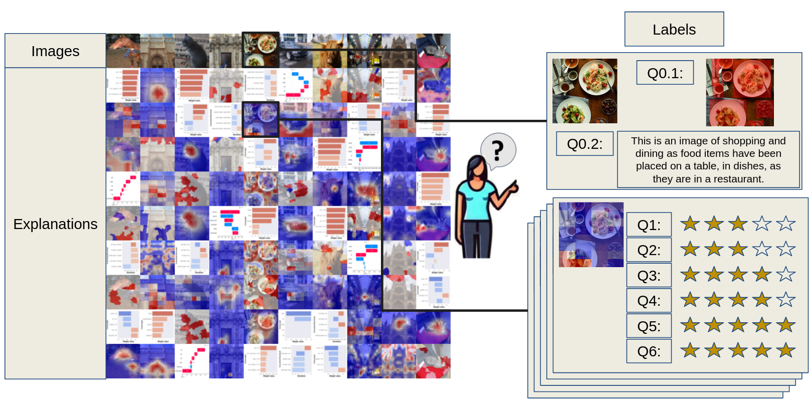
Figure 1: Overview of the human evaluation of the PASTA-dataset. Each image is paired with multiple computed explanations, which are then annotated by human evaluators, first with baseline questions Q0.1 and Q0.2 and then regarding their interpretability and usefulness, using the questions Q1—Q6 outlined in Section 3.4.

3.1 Dataset Composition

To evaluate the performance of different perceptual metrics, we collect a large-scale dataset composed of images of four highly heterogeneous datasets: COCO (Lin et al., 2014), Pascal Part (Chen et al., 2014), Cats Dogs Cars (Kazmierczak et al., 2024), and Monumai (Lamas et al., 2021). This collection is referred to as the classifier’s dataset A.1.1. It is important to distinguish this from the PASTA-dataset, which comprises the final set of images, annotations, labels, and explanations obtained through our evaluation process. Each dataset includes two levels of annotations: image-based annotations and concept-based annotations. This dual-level annotation framework allows for the application of Concept-Based and other XAI methods, enabling a robust evaluation across different approaches. For this, we use for the computation of explanations a subset of 25 images of the classifier’s dataset test split per dataset, resulting in a comprehensive evaluation of 100 images, that serve as the basis of the PASTA-dataset. This diverse selection ensures a broader generalization of the XAI techniques across datasets being assessed. Note that, unlike traditional datasets, our benchmark dataset comprises a triplet of images, explanations, and labels. This triplet enables us to quantitatively assess the quality of XAI techniques (see Figure 1).

3.2 XAI Methods

To ensure representativity, we consider two distinct types of explanations. The first type comprises saliency methods, which generate explanations by assigning an importance score to each pixel of the input image, indicating the significance of each pixel in the prediction process. The second type consists of concept-based explanations, which highlight the importance of human-understandable concepts in the explanation. A detailed list of the methods and more details on each technique are given in Appendix A.2.

Among saliency-based methods, we consider model-agnostic explanations (LIME (Ribeiro et al., 2016) and SHAP (Lundberg & Lee, 2017)), gradient-based (FullGrad (Srinivas & Fleuret, 2019)) and model-specific techniques. The model-specific methods include GradCAM (Selvaraju et al., 2017), HiResCAM (Draelos & Carin, 2020), GradCAMElementWise (Pillai & Pirsiavash, 2021), GradCAM++ (Chattopadhay et al., 2018), XGradCAM (Fu et al., 2020), AblationCAM (Ramaswamy et al., 2020), ScoreCAM (Wang et al., 2020), EigenCAM (Muhammad & Yeasin, 2020), EigenGradCAM (Muhammad & Yeasin, 2020), LayerCAM (Jiang et al., 2021), Deep Feature Factorizations (Collins et al., 2018), and BCos (Böhle et al., 2024).

Among concept-based methods, we explore those that produce explanations through counterfactuals (CLIP-QDA-sample (Kazmierczak et al., 2024)), and feature importance (X-NeSyL (Díaz-Rodríguez et al., 2022), LaBo (Yang et al., 2023), CLIP-linear (Yan et al., 2023), LIME-CBM (Kazmierczak et al., 2024), RISE (Petsiuk et al., 2018) and SHAP-CBM (Kazmierczak et al., 2024)). Additionally, we employ various strategies for concept extraction: zero-shot methods, training from concept annotations, and training from bounding boxes.

3.3 Training Classifiers and Computing the XAI Dataset

The initial phase in constructing the sample set involves training the various classifier models on which explanations will be generated. Specifically, we utilize ResNet50 (He et al., 2016), ViT-B (Dosovitskiy, 2020), ResNet50-BCos (Böhle et al., 2024), CLIP-Linear (Yan et al., 2023), CLIP-QDA (Kazmierczak et al., 2024), X-NeSyL (Díaz-Rodríguez et al., 2022), and ConceptBottleneck (Koh et al., 2020). These models are trained separately on the four datasets. Further details regarding the datasets and training procedures are provided in Section A.1 . The final assessment of XAI techniques is conducted on samples of the test set. To provide a diverse range of explanations, our framework incorporates both black-box models, explained using post-hoc methods, and ante-hoc methods, specifically CBMs. The specific details regarding these two families of methods are presented in Appendix A.1.2.

Our codebase includes the 21 XAI methods described in Sect. 3.2 and the 7 backbone models described above. Some XAI methods are incompatible with certain backbones, see Table 6, this leaves 46 distinct combinations of XAI methods and backbones, which we refer to as XAI techniques. We apply each technique to 100 images. This leads to an XAI dataset of 4600 instances, each of which is associated with an image and its ground truth label, the label prediction from a classifier instance, and the explanation from a particular XAI technique. In the next section, we present an approach for evaluating the human perception of these instances.

3.4 Human evaluation protocol

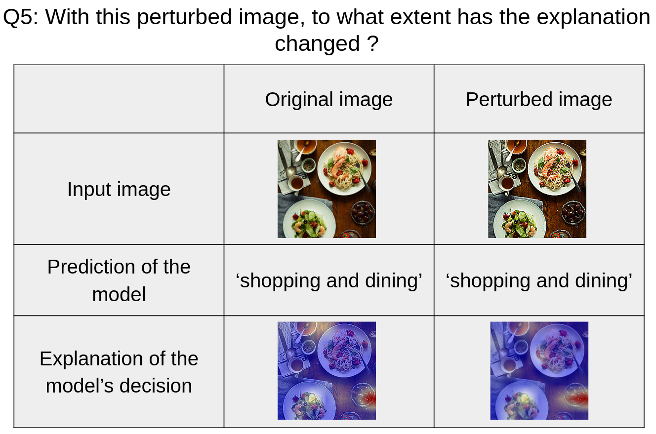
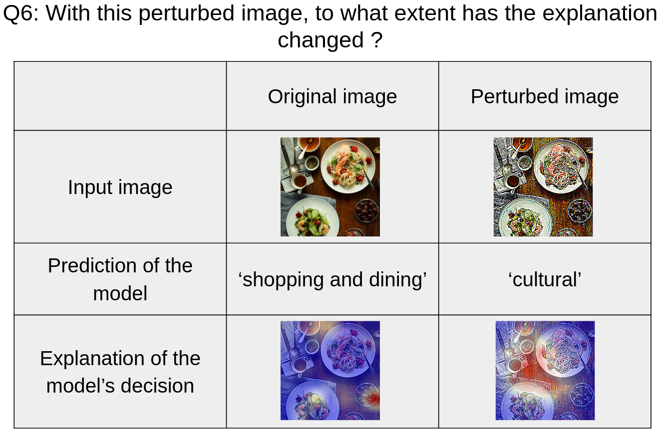
Figure 2: Samples corresponding to questions 5 and 6. On the left, a light perturbation is applied, resulting in no label change. On the right, a strong perturbation is applied, leading to a label change.

We aim to quantify the interpretability and usefulness of XAI techniques accurately, using a human evaluation of the quality of evaluations. The resulting dataset serves as a benchmark, enabling us to compare and validate current and future XAI methods. Our human-centric approach complements existing approaches that focus primarily on assessing the model’s internal behavior. For example, traditional evaluations of faithfulness measure how closely an explanation corresponds to the model’s true functioning while we assess in our dataset how the explanation fit human expectations.

We take a structured approach to ensure that the explanations are not only technically sound but also align with human cognitive processes and expectations, fostering the development of more transparent and interpretable AI systems. First, we establish a comprehensive set of assessment criteria that are evaluated on a graded scale. Then, we apply a meticulous evaluation protocol, developed with the help of a psychologist, to ensure that annotators fully understand the task and the expectations. This includes annotator training and close monitoring throughout the process.

Evaluation Criteria

We consolidate different criteria from the literature into the following set of desiderata for XAI explanations that we wish to evaluate (for details, see Appendix B.1):

• Faithfulness (Arrieta et al., 2020; Fel et al., 2022b) measures the extent to which an explanation accurately reflects the true behavior of the model.

• Robustness (Doshi-Velez & Kim, 2017) assesses the stability and relevance of the explanation across a broad range of models and inputs.

• Complexity (Nauta et al., 2023) checks whether the explanation is both simple and informative, balancing clarity and detail.

• Objectivity (Bennetot et al., 2022) evaluates whether the explanation is interpreted consistently by the majority within a given audience.

Evaluation Protocol

Gathering human preferences from surveys is an active field of research in psychology (Fowler Jr, 2013), but also in the field of machine learning e.g., with the recent advent of reinforcement learning from human feedback (RLHF) (Kaufmann et al., 2023). Interfaces, as well as the formulation of questions, play a key role in the quality of the annotations (Pommeranz et al., 2012), and their design must be considered seriously in order to avoid cognitive biases. The following human evaluation protocol has been designed with the help of a psychologist. The formulation of the questions has been carefully chosen to ensure that they are fully understood by each annotator.

To maintain consistency and reliability, all annotators undergo a training session before starting the actual annotation task. This training familiarizes them with the XAI techniques, evaluation criteria, rating scale, and datasets, ensuring a uniform understanding of the task and the expectations. More details about the annotation protocol are given in Appendix A.3, including an example of how questions are presented to the annotators (Fig. 9).

During the evaluation process, annotators are shown an image, a prediction, and an explanation. They are then asked a list of questions that we now describe in more detail. A first set of questions aims at having annotators establish a baseline, i.e., by interpreting and explaining what makes an image recognizable as a specific object or class. This prompts the human annotator to think about what they are relying on to classify the image themselves, before having to evaluate explanations produced by the XAI techniques. The first two questions in the annotation process are:

• Q0.1: What part makes you classify this image as ***? (write an explanation extracting concepts)

• Q0.2: What part of the input helps the prediction? (draw bounding boxes on the image)

Each explanation generated by the XAI techniques is then evaluated regarding each of the desiderata given above (indicated in italics):

• Q1: The provided explanation is consistent with how I would explain the predicted class? Fidelity

• Q2: Overall the explanation provided for the model prediction can be trusted? Complexity

• Q3: Is the explanation easy to understand? Complexity

• Q4: The explanation can be understood by a large number of people, independently of their demographics (age, gender, country, etc.) and culture? Objectivity

• Q5: With this perturbed image, to what extent has the explanation changed ? (Examples with good predictions and light perturbations) Robustness

• Q6: With this perturbed image, to what extent has the explanation changed? (Examples with bad predictions and strong perturbations) Robustness

Annotators evaluate how well the explanations conform to their expectations (Q1), whether the explanations are clear (Q2 and Q3), and if they would rely on these explanations (Q4). They also assess how much the explanations change when the images are perturbed (Q5 and Q6), for both accurate and inaccurate predictions, as studied by (Fel et al., 2022b). An example is shown in Figure 2. Each explanation is rated on a scale from one to five stars, where one star indicates the explanation is entirely uncorrelated with the annotator’s reasoning, and five stars represent perfect correlation. This star rating system allows for a nuanced assessment of the quality of the explanations, reflecting how closely they align with human understanding.

3.5 Human Evaluation and Results

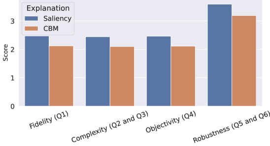
(a) Scores for each question, for saliency-based and CBM-based explanation

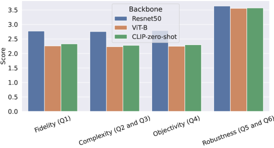
(b) Scores for each question, for different backbones of saliency methods

Figure 3: Comparison of explanation methods and backbones: Overall, saliency methods are preferred over CBM-based explanations. As backbones for saliency methods, ViT-B and CLIP obtain overall similar results, while Resnet50 has better scores.

We now present a brief summary of the human evaluations obtained in the PASTA-dataset, using the previously described protocol. Full results and values are available in Appendices B.2 and B.3. Our XAI dataset, described in Sect. 3.3, contains 4600 instances with images, predictions, and explanations. From this set, we select 2200 samples randomly for the saliency maps as detailed in Appendix A.1 and let them be evaluated by humans according to the protocol above. Each instance receives five evaluations from different annotators. We aggregate these evaluations using majority voting to favor consensus opinions.

As illustrated by Figure 3(a), we observe that these results indicate a preference for image-based techniques, suggesting that saliency maps are perceived as more interpretable than CBMs. Additionally, Figure 3(b) shows the average score among techniques that share the same backbone. Interestingly, CLIP and ViT have similar scores, likely due to the architectural similarities between the two models. ResNet 50, which played a pivotal role in the development of many XAI methods, consistently scores higher. This could suggest a potential bias toward ResNet 50 in the design and effectiveness of current XAI methods.

3.6 Correlation with other metrics.

We turn to the question of how the human scores in the PASTA-dataset correlate with standard XAI metrics. An analysis based on the Pearson Correlation Coefficient and the Spearman rank Correlation Coefficient for different perturbation strategies, shown in Table 1 indicates a rather weak correlation between human scores and ROAD (Rong et al., 2022), a popular metric to evaluate faithfulness. We conclude that our human scores indeed cover an aspect of explanation quality unrelated to that of perceptual quality, as predicted by Biessmann & Refiano (2021). Additional results, including results for other axioms, are available in Appendix B.1 and B.2.

Table 1: Pearson Correlation Coefficient (PCC) and Spearman rank Correlation Coefficient (SCC) between faithfulness computed with different perturbation strategies and human scores. In parentheses, the respective p-values.

	ROAD		Black patches		Uniform noise		Gaussian noise
	PCC	SCC	PCC	SCC	PCC	SCC	PCC	SCC
Q1	0.01 (0.62)	-0.04 (0.12)	0.06 (0.02)	0.05 (0.04)	0.07 (0.01)	0.03 (0.24)	0.07 (0.02)	0.02 (0.38)
Q2	-0.01 (0.88)	-0.03 (0.20)	0.04 (0.19)	0.04 (0.17)	0.06 (0.04)	0.02 (0.45)	0.05 (0.08)	0.01 ( 0.63)
Q3	0.03 (0.33)	-0.03 (0.34)	0.04 (0.10)	0.04 (0.16)	0.08 (0.01)	0.04 (0.13)	0.06 (0.02)	0.03 (0.30)
Q4	0.03 (0.25)	-0.04 (0.17)	0.04 (0.19)	0.03 (0.33)	0.08 (0.01)	0.03 (0.21)	0.06 (0.02)	0.02 (0.41)
Q5	-0.05 (0.05)	0.02 (0.41)	0.01 (0.93)	0.04 (0.14)	-0.05 (0.07)	-0.01 (0.78)	-0.04 (0.16)	0.01 (0.95)
Q6	-0.02 (0.37)	0.06 (0.03)	-0.13 (1e-5)	-0.08 (0.01)	-0.04 (0.16)	-0.01 (0.68)	-0.04 (0.13)	-0.01 (0.79)

4 Developing a Metric for Perceptual Evaluation

Our human preference dataset contains evaluations of the fidelity, complexity, objectivity, and robustness of each evaluation. These scores were painstakingly attributed by human annotators. To provide a tool for measuring human assessment of XAI techniques, we introduce a model, the PASTA-metric, which simulates human evaluation. The global pipeline is illustrated in Figure 4. More precisely, the PASTA-metric is composed of an embedding network (Section 4.1), that processes both CBM outputs or saliency maps, and a scoring network (Section 4.2), that computes scores from the embeddings. Further details on the implementation are given in Appendix C.1. Using the data collected in Section 3, the PASTA-metric aims at predicting the human scores for questions 1 to 6, aggregated by majority voting.

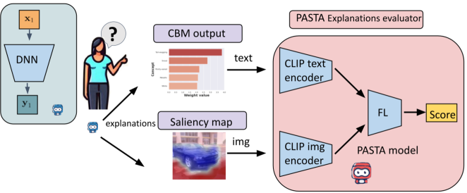
Figure 4: Pipeline of the PASTA-metric. Initially, embeddings are computed based on the explanations. Then a scoring network, trained on labels provided by the Benchmark Dataset, generates a final score.

4.1 Computation of embeddings

Drawing inspiration from recent literature in automated scoring (Yang et al., 2020; Wang et al., 2022b), we use a foundation model to generate embeddings. Given its multimodal capabilities, we select CLIP (Yan et al., 2023) as the embedding model. This choice allows for a unified integration of both concept-based explanations, which can be transformed into text, and saliency map-based explanations, which can be projected into the same embedding space.

Let us denote by ${\bm{x}}_{i}\in\mathbb{R}^{H\times W\times 3}$ the $i$-th test image of height $H$ and width $W$ in the dataset and by ${\bm{e}}_{i}^{saliency}\in\mathbb{R}^{H\times W}$ any explanation produced by a saliency-based XAI method for this image. We also note the CLIP image encoder as $\text{CLIP}_{\text{image}}$. For saliency explanations, the resulting embedding based on a saliency map can be obtained using the following formula:

$$\phi_{\text{image}}({\bm{e}}_{i}^{saliency})=\text{CLIP}_{\text{image}}(Heatmap({\bm{x}}_{i},{\bm{e}}_{i}^{saliency})),$$ (1)

where $Heatmap$ is the process generating the saliency related heatmap to the image. More details are given in Appendix C.3.1.

For CBMs, let us denote with ${\bm{e}}_{i}^{CBM}\in\mathbb{R}^{K}$ any explanation produced by a saliency-based XAI method for this image ${\bm{x}}_{i}$, where $K$ is the length of the concept set. These attributions are converted into a sentence, which is then embedded. Let $\text{CLIP}_{\text{text}}$ denote the CLIP text encoder and $Sentence$ the process of converting the CBM explanation into text, more details about which $Sentence$ are given in Appendix C.3.1. The resulting embedding is:

$$\phi_{\text{text}}({\bm{e}}_{i}^{CBM})=\text{CLIP}_{\text{text}}(Sentence({\bm{e}}_{i}^{CBM}))\,.$$ (2)

4.2 Scoring network

Once the embeddings are computed, a scoring network composed of a linear layer is used to predict scores. Inspired by Automated Essay Scoring  (Yang et al., 2020; Wang et al., 2022b), we use a loss $L$ that combines a similarity loss $L_{s}$, a mean squared error (MSE) loss $L_{mse}$, and a ranking loss $L_{r}$. From a set of ground truth scores obtained from majority voting $\{m_{k}\}_{k\in[0,N_{s}]}$ and the predictions given by the scoring network $\{\hat{m}_{k}\}_{k\in[0,N_{s}]}$, the resulting loss is defined as:

$$L=\alpha L_{s}+\beta L_{mse}+\gamma L_{r},$$ (3)

where $\alpha$, $\beta$, and $\gamma$ are hyperparameters controlling the relative importance of each component. Details about the different losses are given in Appendix C.3

4.3 Classifier results

In all experiments, we employed the Adam optimizer with a batch size of 128, training for 500 epochs at a learning rate of 0.001. Additionally, we configured the parameters as follows: $\alpha$ was set to 1, $\beta$ to 0.01, and $\gamma$ to 0.1. We split our dataset in $1540$ training samples, $330$ validation samples, and $330$ testing samples. The experiments were conducted using a V100-16GB GPU. The training and inference times are summarized in Table 2. It is important to note that, for both inference and testing, the majority of the computational time is dedicated to precomputing CLIP embeddings, as the scoring network itself is relatively lightweight and requires minimal computational resources.

Table 2: Training and Inference Times on GPU and CPU.

Device	Training Time (s)	Inference Time (s)
GPU	214.18	8.89
CPU	1308.84	57.52

For questions 1 to 6 in Section 3, we calculated the Mean Square Error (MSE), Quadratic Weighted Kappa (QWK), and Spearman Correlation Coefficient (SCC) between the predicted and ground truth labels on the test set. The results are presented in Table 3. Additional details about these computations can be found in Appendix C.1.2. For comparison, we also include the scores from a linear regression model and report the inter-annotator agreement values, which correspond to the metrics computed between a randomly selected annotator’s score and the mode. Additional experiments, including ablation studies, are presented in Appendix C.2.

Table 3: Mean Square Error, Quadratic Weighted Kappa and Spearman Correlation Coefficient for each question. Each value is the average result on 5 runs with the standard deviation. Human here stands for the inter-annotator agreement.

Regressor	Quest.	MSE	QWK	SCC
CLIP+Linear Regression	Q1	1.48 $\pm$ 0.13	0.37 $\pm$ 0.04	0.19 $\pm$ 0.19
PASTA	Q1	0.85 $\pm$ 0.06	0.55 $\pm$ 0.04	0.28 $\pm$ 0.28
Human	Q1	0.53 $\pm$ 0.03	0.73 $\pm$ 0.03	0.37 $\pm$ 0.37
CLIP+Linear Regression	Q2	1.45 $\pm$ 0.14	0.36 $\pm$ 0.04	0.19 $\pm$ 0.19
PASTA	Q2	0.86 $\pm$ 0.06	0.54 $\pm$ 0.03	0.28 $\pm$ 0.28
Human	Q2	0.51 $\pm$ 0.05	0.74 $\pm$ 0.02	0.38 $\pm$ 0.38
CLIP+Linear Regression	Q3	1.55 $\pm$ 0.14	0.33 $\pm$ 0.03	0.17 $\pm$ 0.17
PASTA	Q3	0.96 $\pm$ 0.10	0.51 $\pm$ 0.05	0.26 $\pm$ 0.26
Human	Q3	0.74 $\pm$ 0.03	0.63 $\pm$ 0.02	0.33 $\pm$ 0.33
CLIP+Linear Regression	Q4	1.46 $\pm$ 0.10	0.34 $\pm$ 0.05	0.18 $\pm$ 0.18
PASTA	Q4	0.90 $\pm$ 0.05	0.52 $\pm$ 0.03	0.27 $\pm$ 0.27
Human	Q4	0.72 $\pm$ 0.02	0.62 $\pm$ 0.02	0.33 $\pm$ 0.33
CLIP+Linear Regression	Q5	2.82 $\pm$ 0.22	0.14 $\pm$ 0.05	0.10 $\pm$ 0.08
PASTA	Q5	1.86 $\pm$ 0.16	0.29 $\pm$ 0.08	0.15 $\pm$ 0.16
Human	Q5	1.00 $\pm$ 0.06	0.65 $\pm$ 0.03	0.34 $\pm$ 0.34
CLIP+Linear Regression	Q6	1.02 $\pm$ 0.06	0.32 $\pm$ 0.05	0.15 $\pm$ 0.16
PASTA	Q6	0.67 $\pm$ 0.09	0.51 $\pm$ 0.08	0.25 $\pm$ 0.26
Human	Q6	0.52 $\pm$ 0.03	0.59 $\pm$ 0.02	0.29 $\pm$ 0.29

4.4 Generalization capabilities of the PASTA-metric

In the main study, to constitute training, validation, and test sets, we shuffled all the samples without considering the XAI technique or the dataset they belong to. This means that the same images with different XAI techniques, or the same XAI techniques applied to different images, possibly from the same dataset, could be found in the training and test set. In this section, we investigate the impact of shuffling solely the image indices and the explanation indices. By doing so, we ensure that samples from the same image (resp. same XAI technique) cannot be in two different splits. This will help us investigate the generalization capabilities of the model in two distinct ways: can it generalize to new XAI techniques, and to new images? The results of the two setups for Q1 are shown in Table 4. The results indicate a decrease of 0.04 in QWK when shuffling across XAI techniques and a more significant drop of 0.07 when shuffling across image IDs. This opens a discussion on the potential for applying the PASTA-metric to other image datasets. Regarding the generalization to new XAI methods, the relatively moderate drop in performance supports the feasibility of testing our metric on novel XAI techniques.

Table 4: Summary of results for different restrictions applied during dataset splitting. The label No indicates no restrictions, Img id denotes that the same image indices $i$ are maintained across splits, and XAI id indicates that the same explanation indices $j$ are preserved in different splits. Each value is the average result on 5 runs with the standard deviation.

Restriction split	MSE	QWK	SCC
No	0.85 $\pm$ 0.06	0.55 $\pm$ 0.04	0.28 $\pm$ 0.28
xai_id	0.96 $\pm$ 0.10	0.51 $\pm$ 0.05	0.26 $\pm$ 0.26
img_id	1.06 $\pm$ 0.05	0.48 $\pm$ 0.05	0.25 $\pm$ 0.25

5 Conclusions

In this paper, we introduce PASTA, a novel perceptual assessment system designed to benchmark explainable AI (XAI) techniques in a human-centric manner. We integrate four diverse datasets — COCO, Pascal Parts, Cats Dogs Cars, and Monumai — to form a large-scale benchmark dataset for XAI, and used it for an assessment of XAI explanations by human annotators. We also develop an automated evaluation metric that mimics human preferences based on a comprehensive database of human evaluations. This framework offers a scalable and reliable way to compare different XAI methods, facilitating robust evaluations across modalities previously unaddressed.

Our findings demonstrate a clear preference for saliency-based explanations, particularly techniques such as LIME and SHAP, which align well with human intuition. These results affirm the scalability and reliability of our perceptual metric, which provides consistency with human assessment while automating much of the evaluation process.

However, there are limitations to our approach. The current study focuses on a fixed set of datasets and XAI techniques. Human evaluations can be influenced by subjective factors that may affect the consistency of results. Furthermore, annotators can inadvertently introduce biases. Perceptual metrics like the ones proposed here are therefore not intended to serve as absolute measures of XAI performance. Rather, we consider them simply as complementary to other XAI metrics.

Looking ahead, dynamic scoring approaches could be explored to capture the evolving nature of XAI techniques and their use in real-world applications. In conclusion, PASTA intends to take a step towards creating a transparent and trustworthy AI ecosystem. By aligning AI explanations with human cognitive processes, we aim to foster the development of more interpretable AI systems that can be understood and trusted by users across various domains.

1

Table of Contents - Supplementary Material

Appendix A PASTA-dataset: process

A.1 Classifier training

A.1.1 Dataset

The dataset used in PASTA is designed to provide a benchmark for evaluating a wide range of XAI techniques across different explanation modalities. To ensure robustness and versatility, we have built a benchmark dataset consisting of four diverse, publicly available datasets, each bringing distinct characteristics in terms of visual content and concept annotations. Choosing which task to focus on is a tough question. We have chosen to focus on the image classification task. This task can be performed in many different domains, but in order not to be too domain-specific, we decided to work on general datasets. These datasets enable the evaluation of both image-based and concept-based XAI methods.

The dataset used to train our inference model integrates four datasets, each chosen for its unique attributes that align with the requirements of evaluating explainability methods. The datasets are as follows:

• COCO: A widely-used dataset known for its complexity and variety, containing 117k training images, 4.5k validation images annotated with 80 object categories, which we consider to be concepts in the images. The task we focus on is indoor scene labeling, to do so, we took the subset of images of indoor scenes (53,051 images). Then, we labeled the images using a scene label DNN trained on the MIT SUN.

• Pascal Part: This dataset focuses on detailed part-level annotations, providing fine-grained insights into object structure and component relationships. It is composed of 13,192 training images, 39 concepts, and 16 classes.

• Cats Dogs Cars: A curated dataset featuring images of cats, dogs, and cars. The goal of this dataset is to explore if color biases are present in the model or not. It is composed of 3,858 training images, 39 concepts, and 3 classes. Since this network does not include annotated concepts, we used Grounding DINO (Liu et al., 2023) as an annotator.

• Monumai: A specialized dataset containing images of monuments, with annotations that include both the overall structures and specific architectural features. It is composed of 908 images, 15 concepts, and 4 classes.

Each dataset in the classifier’s training datasets is annotated at two levels:

• Image-level annotations: These are traditional class labels or object categories that describe the primary content of the image.

• Concept-level annotations: These describe specific, human-understandable features within the image, enabling the application of Concept Bottleneck Models (CBMs) and other concept-based XAI methods. The list of concepts for each dataset is detailed in Table LABEL:table:table_concepts.

Table 5: List of concepts used in all our CBMs. For each Dataset used, we choose a different set to fit the annotations.

Dataset	Concepts
catsdogscars, pascalpart	engine, artifact_wing, animal_wing, stern, tail, locomotive, arm, hair, wheel, chain_wheel, handlebar, hand, headlight, saddle, body, bodywork, beak, head, eye, foot, leg, neck, torso, cap, license_plate, door, mirror, window, ear, muzzle, horn, nose, hoof, mouth, eyebrow, plant, pot, coach, screen
monumai	horseshoe-arch, lobed-arch, pointed-arch, ogee-arch, trefoil-arch, serliana, solomonic-column, pinnacle-gothic, porthole, broken-pediment, rounded-arch, flat-arch, segmental-pediment, triangular-pediment, lintelled-doorway
coco	person, backpack, umbrella, handbag, tie, suitcase, bicycle, car, motorcycle, airplane, bus, train, truck, boat, traffic light, fire hydrant, stop sign, parking meter, bench, bird, cat, dog, horse, sheep, cow, elephant, bear, zebra, giraffe, frisbee, skis, snowboard, sports ball, kite, baseball bat, baseball glove, skateboard, surfboard, tennis racket, bottle, wine glass, cup, fork, knife, spoon, bowl, banana, apple, sandwich, orange, broccoli, carrot, hot dog, pizza, donut, cake, chair, couch, potted plant, bed, dining table, toilet, tv, laptop, mouse, remote, keyboard, cell phone, microwave, oven, toaster, sink, refrigerator, book, clock, vase, scissors, teddy bear, hair drier, toothbrush

This dual-level annotation setup ensures that XAI methods can be evaluated not only for their ability to explain class predictions but also for how well they handle concept-based explanations. The presence of both granular (part-level, concept) and holistic (object, scene-level) annotations provides a comprehensive evaluation environment for various XAI methods.

In Figure 5, we observe the class distribution across the different datasets. While the distributions are not perfectly uniform, they generally reflect the original composition of the datasets, ensuring that the diversity of the data is preserved in the evaluation process.

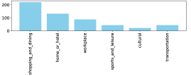
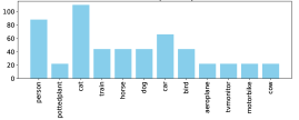
COCO	Pascal Part
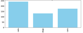
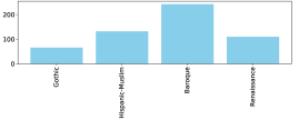
Cats Dogs Cars	Monumai

Figure 5: Class distribution across the different test sets.

A.1.2 Specific procedures for CBMs and black boxes models.

To explain the various training procedures for our CBMs, we decompose them into two components: the concept extractor and the classifier. The concept extractor generates an embedding from an input image, with each element representing a concept, while the classifier predicts the label from this embedding. We categorize the CBMs we use based on the training methods for these two components. For CLIP-based CBMs (LaBo, CLIP-linear, and CLIP-QDA), the concept extraction is performed in a zero-shot manner i.e., we only use the training images and labels to train the classifier. For CBMs that require training the concept extractor, we use the concept annotations provided by each dataset.

For explanations that involve the application of post-hoc techniques on black-box models, we selected the following DNNs: ResNet 50, ViT, and CLIP (zero-shot). For ResNet 50 and ViT, a separate network was trained for each dataset. For CLIP (zero-shot), we followed the standard procedure proposed by Radford et al. (2021), which classifies by selecting the highest similarity score between the image embedding and all the text embeddings. For post-hoc explanations, we directly extract the explanation after training.

A.1.3 Results

As illustrated in Figure 6, the models used in this study achieve an accuracy of at least 59%. Notably, one of the models, the zero-shot CLIP, exhibits difficulty specifically with the Monumai dataset, which explains some of the performance variability. Despite this, the overall accuracy of the models remains relatively consistent across datasets. For CBMs, achieving high accuracy across all models required certain compromises, particularly with respect to the concepts used. Although for uniformity we used the same concept sets across different models, it was not always guaranteed that the trained model is the best model.

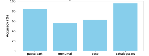
Figure 6: Accuracy across the different test sets of the different models.

A.2 XAI techniques

Table 6 presents an overview of the different XAI methods integrated into the dataset. A brief description of each method is provided below to summarize their key features and mechanisms.

Table 6: XAI methods included in our dataset. Name denotes the identifier of the utilized XAI method. Functioning specifies the mechanism of the explanation computation, including methods that rely on gradient weighting (Gradient), probing reactions to localized perturbations (Perturbation), abstracting activations through factorization (Factorization), leveraging directly interpretable latent spaces (Interpretable latent space), or searching for counterfactuals (Counterfactual). Attribution indicates the data type on which the attribution weights are applied: either on input images (Image) or on a computed representation of the image as concepts (Concepts). Stage indicates whether the explanation is produced by a ante-hoc or a post-hoc process.

Name	Functioning	Attribution on	Stage	Applied on
BCos (Böhle et al., 2024)	Interpretable latent space	Image	Ante-hoc	ResNet50-BCos
GradCAM (Selvaraju et al., 2017)	Gradient	Image	Post-hoc	ViT, ResNet50, CLIP (zero-shot)
HiResCAM (Draelos & Carin, 2020)	Gradient	Image	Post-hoc	ViT, ResNet50, CLIP (zero-shot)
GradCAMElementWise (Pillai & Pirsiavash, 2021)	Gradient	Image	Post-hoc	ViT, ResNet50, CLIP (zero-shot)
GradCAM++ (Chattopadhay et al., 2018)	Gradient	Image	Post-hoc	ViT, ResNet50, CLIP (zero-shot)
XGradCAM (Fu et al., 2020)	Gradient	Image	Post-hoc	ViT, ResNet50, CLIP (zero-shot)
AblationCAM (Ramaswamy et al., 2020)	Perturbation	Image	Post-hoc	ViT, ResNet50, CLIP (zero-shot)
ScoreCAM (Wang et al., 2020)	Perturbation	Image	Post-hoc	ViT, ResNet50
EigenCAM (Muhammad & Yeasin, 2020)	Factorization	Image	Post-hoc	ViT, ResNet50, CLIP (zero-shot)
EigenGradCAM (Muhammad & Yeasin, 2020)	Gradient+Factorization	Image	Post-hoc	ViT, ResNet50, CLIP (zero-shot)
LayerCAM (Jiang et al., 2021)	Gradient	Image	Post-hoc	ViT, ResNet50, CLIP (zero-shot)
FullGrad (Srinivas & Fleuret, 2019)	Gradient	Image	Post-hoc	ViT, ResNet50
Deep Feature Factorizations (Collins et al., 2018)	Factorization	Image	Post-hoc	ViT, ResNet50, CLIP (zero-shot)
SHAP (Lundberg & Lee, 2017)	Perturbation	Image	Post-hoc	ViT, ResNet50, CLIP (zero-shot)
LIME (Ribeiro et al., 2016)	Perturbation	Image	Post-hoc	ViT, ResNet50, CLIP (zero-shot)
X-NeSyL (Díaz-Rodríguez et al., 2022)	Interpretable latent space	Concepts	Ante-hoc	X-NeSyL
CLIP-linear-sample (Yan et al., 2023)	Interpretable latent space	Concepts	Ante-hoc	CLIP-linear
CLIP-QDA-sample (Kazmierczak et al., 2024)	Counterfactual	Concepts	Ante-hoc	CLIP-QDA
LIME-CBM (Kazmierczak et al., 2024)	Perturbation	Concepts	Post-hoc	CLIP-QDA, ConceptBottleneck
SHAP-CBM (Kazmierczak et al., 2024)	Perturbation	Concepts	Post-hoc	CLIP-QDA, ConceptBottleneck
RISE (Petsiuk et al., 2018)	Perturbation	Concepts	Post-hoc	ConceptBottleneck

LIME (Local Interpretable Model-agnostic Explanations): LIME explains individual predictions of any classifier by approximating it locally with an interpretable model. It perturbs the input and observes how the predictions change, identifying the most influential parts of the input for the prediction. This is a saliency-based XAI method, visualizing the important regions in an image that the DNN relies on.

SHAP (SHapley Additive exPlanations): SHAP is a unified approach to interpreting model predictions based on Shapley values from cooperative game theory. It assigns each feature an importance value for a particular prediction, offering a sound measure of feature importance. This is a saliency-based XAI method, visualizing the important regions in an image that the DNN relies on.

GradCAM (Gradient-weighted Class Activation Mapping): GradCAM visualizes the regions in an image that contribute to the classification. It uses the gradients of the target concept (e.g., a specific class) flowing into the final convolutional layer to produce a coarse localization map highlighting important regions. This is a saliency-based XAI method.

AblationCAM: AblationCAM improves GradCAM by iteratively removing parts of the input and observing the output effect to identify important regions. This is a saliency-based XAI method, visualizing the crucial regions in an image that the DNN relies on.

EigenCAM: EigenCAM applies PCA to the activations of the last convolutional layer to produce a saliency map. It highlights the directions in which activations show the most variance, identifying critical features. This is a saliency-based XAI method.

FullGrad: FullGrad computes gradients of the output with respect to both the input and intermediate layer outputs, aggregating these gradients to generate a comprehensive saliency map. It is a saliency-based XAI method that visualizes key regions in an image.

GradCAMPlusPlus: GradCAMPlusPlus improves GradCAM with a refined weighting scheme for the gradients, allowing better handling of multiple occurrences of the target concept. This is a saliency-based XAI method.

GradCAMElementWise: GradCAMElementWise extends GradCAM by considering element-wise multiplications of gradients and activations, producing more precise visual explanations. This is a saliency-based XAI method.

HiResCAM: HiResCAM improves on class activation mapping by using higher-resolution feature maps for more detailed visual explanations. This is a saliency-based XAI method.

ScoreCAM: ScoreCAM improves CAM methods by using output scores to weight the activation maps’ importance, providing a more faithful saliency map without relying on gradients. This is a saliency-based XAI method.

XGradCAM: XGradCAM integrates cross-layer information to combine saliency maps from different layers, producing a more comprehensive explanation. This is a saliency-based XAI method.

DeepFeatureFactorization: This method decomposes feature representations learned by a deep model into interpretable factors. It provides insights into how features contribute to the model’s decisions, being a saliency-based XAI method.

CLIP-QDA-sample: This model uses the CLIP framework and applies Quadratic Discriminant Analysis (QDA) for classification. It links visual and concept-based representations to provide interpretable explanations. This is a concept bottleneck model (CBM).

CLIP-Linear-sample: Similar to CLIP-QDA, this model leverages the CLIP framework but applies logistic regression for classification, providing interpretable explanations based on concept representations. This is a CBM.

X-NeSyL: X-NeSyL identifies concepts using object detection and applies a small DNN to these concepts, using the weights assigned to each concept for explanation.

LIME CBM: This model generates a list of concepts and applies logistic regression. It uses LIME to highlight the most important concepts for classification.

SHAP CBM: This model generates a list of concepts and applies logistic regression, using SHAP to emphasize the most crucial concepts in classification.

Labo: Labo extracts human-interpretable concepts and maps them to the model’s internal representations for more comprehensible decision-making explanations.

RISE (Randomized Input Sampling for Explanation): RISE generates heatmaps by perturbing input regions and measuring their impact on model outputs. This technique identifies the most influential regions in the model’s decision-making process.

BCos: BCos introduces specific layers to encourage alignment between weights and activation maps, which can then be used for explainability.

Finally, Figure 7 shows the distribution of XAI techniques applied across the datasets. To enhance the generalizability of our results, we increased the diversity of XAI techniques used. This was achieved by not applying every technique to every image uniformly, allowing for a more diverse set of explanations to be generated. This variability ensures that our analysis captures a broad spectrum of interpretability techniques, providing deeper insights into the performance of XAI techniques across different datasets and models.

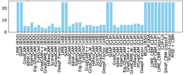
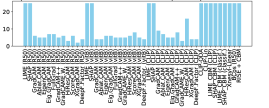
COCO	Pascal Part
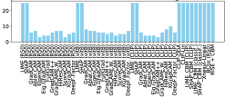
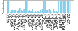
Cats Dogs Cars	Monumai

Figure 7: Distribution across the different XAI techniques across the different datasets.

A.3 Dataset Annotation process

The annotation process took place via an online web application, created and deployed by a contracting company. 15 participants were recruited to take part in the annotation process. These participants ranged in age from 19 to 37 (mean age 25.9, standard deviation 5.5). Figure 8 shows the age distribution. Among the participants, 5 identified themselves as male, 10 as female, 0 as non-binary, 0 did not wish to say. All participants were based in India.

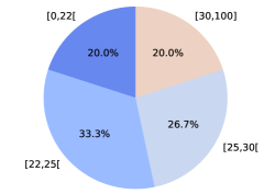
Figure 8: Age distribution of the annotators.

Each participant’s task was to annotate 147 explanations. For each image, participants had to explain what led them to classify the displayed image as the model’s prediction. Participants responded openly using a text form. Similarly, they were asked to describe the elements of the image that helped them make the decision to classify the image as the model did. These two questions (Q0.1 and Q0.2) are used to establish a baseline for interpreting what makes an image recognizable as a specific object or class, and what are the salient features of the images that would explain this choice.

Once they had answered these two questions, they moved on to the next screen, where they had to answer a series of 6 questions (see Figure 9 showing a screenshot of the interface with the original image slightly perturbed). The questions concerned different sections of the screen. The first four questions (Q1 to Q4) concerned Section 1, which showed the original image on the left and the explanation on the right. These first four questions enabled participants to assess the levels of reliability, complexity and objectivity of the explanation. The fifth question (Q5) concerned Section 2, showing the slightly disturbed original image and the corresponding explanation. The sixth question (Q6) concerned Section 3, showing a more disturbed image and the corresponding explanation. These last two questions were intended to assess the robustness of the XAI technique. For each question, participants had to answer with a 5-point Likert scale.

All questions were formulated in collaboration with psychologists to enhance the quality of human feedback. Our aim was to avoid influencing responses and to eliminate any ambiguities that could lead to inaccurate answers. Human decision-making, especially when it involves assessing the quality of explanations, is complex. To address this, we provided training on deep learning and various XAI techniques, ensuring the content was clearly understandable by the annotators. After the initial training, the annotators answered the questions, and we held weekly meetings to clarify any confusion they encountered

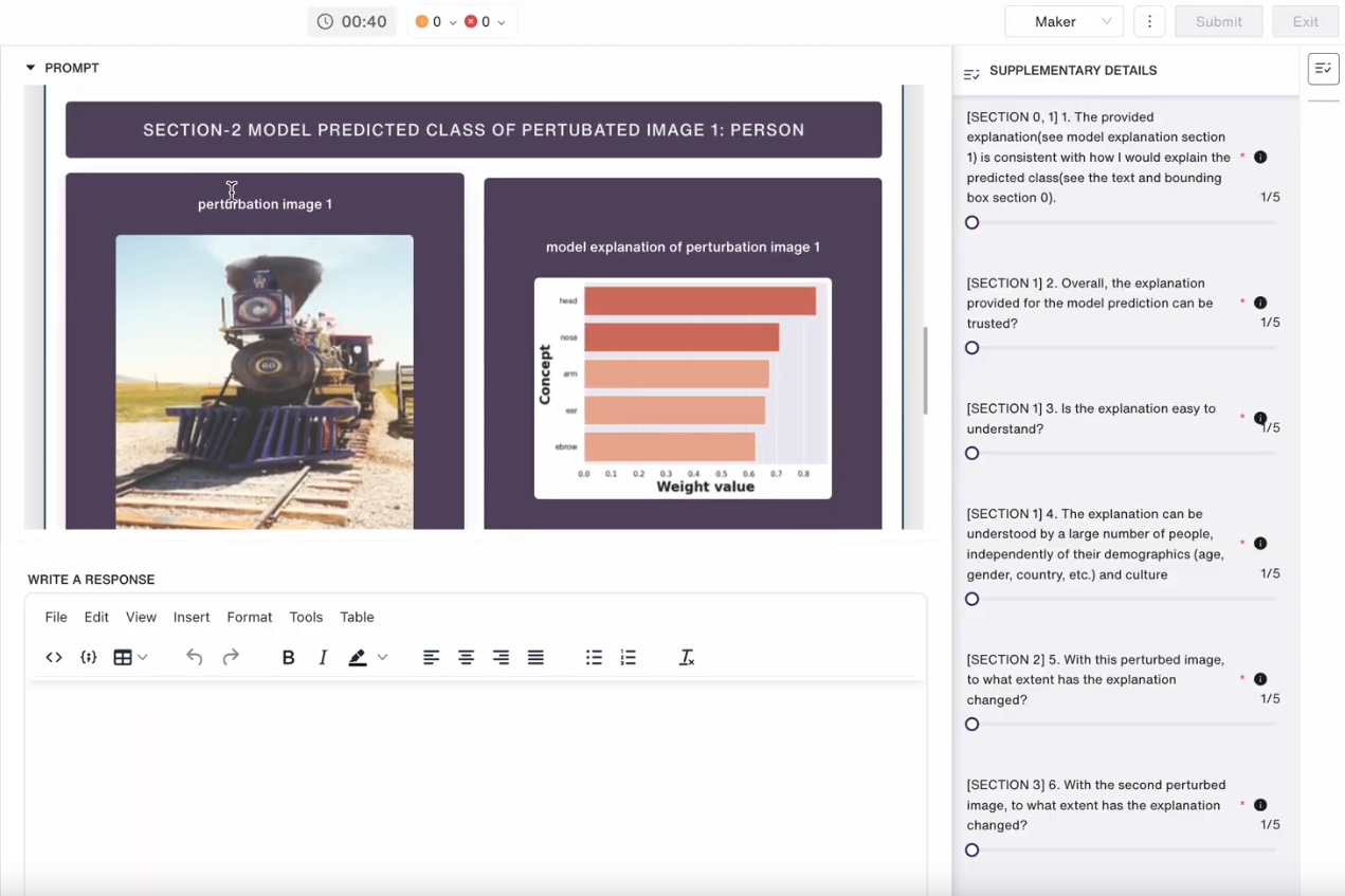
Figure 9: Screenshot of the annotation interface. Questions are on the right-part of the interface. Middle panel shows Section 2: slightly disturbed original image with the explanation.

Appendix B PASTA-dataset: additional experiments

B.1 Comparison with existing metrics

Evaluating the quality of an explanation typically involves estimating different and potentially orthogonal aspects of it. In addition to the perceptual quality addressed in this work, others can be numerically simulated by having access to model weights. In this additional analysis, we consider some of those aspects and measure how much they correlate with human scores. The results cover only image-level attribution methods (see Table 6), as CBMs do not support such kinds of input-level manipulations.

Faithfulness:

How much does the explanation describe the true behavior of the model? A number of different ways to compute faithfulness exist, but they all broadly fit the same framework of measuring how much model predictions change in response to input perturbations (Bhatt et al., 2021; Alvarez-Melis & Jaakkola, 2018a; Yeh et al., 2019; Rieger & Hansen, 2020; Arya et al., 2019; Nguyen & Martínez, 2020; Bach et al., 2015; Samek et al., 2016; Montavon et al., 2018; Ancona et al., 2017; Dasgupta et al., 2022). Intuitively, an explanation is faithful if perturbing regions deemed irrelevant by the explanation bring little to no change in model output, whereas perturbing regions deemed relevant bring a considerable change. In this analysis, we resort to the evaluation protocol outlined in Azzolin et al. (2024), which generalized a number of common faithfulness metrics into a common mold. Specifically, faithfulness is estimated as the harmonic mean of sufficiency and necessity, which account for the degree of prediction changes after perturbing irrelevant or relevant portions of the input, respectively. There is no unique way of applying perturbations to an image, and different techniques are oftentimes reported to give different interpretations (Hase et al., 2024; Rong et al., 2022). To avoid this confounding effect, we report the results for three different baseline perturbations, namely uniform and Gaussian noise, and black patches, along with a more advanced information-theoretic strategy named ROAD (Rong et al., 2022). Since explanations are oftentimes in the form of soft relevance scores over the entire input, a threshold is needed to tell apart relevant from irrelevant image regions. To avoid relying upon this hard-to-define hyperparameter, we aggregate the scores across multiple thresholds keeping only the best value. Therefore, for each threshold value, pixels are sorted based on their relevance and progressively perturbed until reaching the fixed threshold value, while leaving the others unchanged. Then, we measure the absolute difference in class-predicted confidence between clean and perturbed images, normalizing the results to ensure that both are the higher the better. The area under the curve is finally computed, indicating how fast the model changes its predictions with respect to the amount of perturbed pixels.

Robustness:

Robustness roughly refers to how stable the explanation is to small input perturbations. Different ways to estimate it exist (Alvarez-Melis & Jaakkola, 2018b; Montavon et al., 2018; Yeh et al., 2019; Dasgupta et al., 2022; Agarwal et al., 2022a). In our analysis, we focused on MaxSensitivity (Yeh et al., 2019), which applies random input perturbations to the entire image and measures the pixel-wise difference between the original explanation, and the one obtained on the perturbed sample. Again, different perturbation techniques can be applied, and we resort to the two simple baselines, namely uniform and Gaussian noise. No normalization is applied, therefore the values are the higher the worse. More advanced techniques like ROAD (Rong et al., 2022) cannot be applied in this context, since the perturbation is applied uniformly over the entire image. In Table 7, we report the correlation between MaxSensitivity and human scores, outlining a non-significant correlation with the metric and some questions. Surprisingly, the most correlated questions are Q1-4, which are not requesting humans to assess the stability of the explanation, something instead partially addressed by Q5 and Q6. However, the correlation is very weak anyway, questioning any further claims.

Table 7: Pearson Correlation Coefficient (PCC) and Spearman rank Correlation Coefficient (SCC) between MaxSensitivity computed with different perturbation strategies and human scores. In parentheses, the respective p-values.

	Uniform noise		Gaussian noise
	PCC	SCC	PCC	SCC
Q1	-0.30 (1e-5)	-0.37 (1e-5)	-0.30 (1e-5)	-0.35 (0.04)
Q2	-0.30 (1e-5)	-0.36 (1e-5)	-0.28 (1e-5)	-0.33 (0.17)
Q3	-0.30 (1e-5)	-0.36 (1e-5)	-0.29 (1e-5)	-0.34 (0.16)
Q4	-0.29 (1e-5)	-0.36 (1e-5)	-0.28 (0.19)	-0.33 (0.33)
Q5	0.01 (0.72)	0.01 (0.80)	-0.04 (0.89)	-0.09 (0.01)
Q6	0.10 (1e-3)	0.10 (1e-3)	0.09 (0.01)	0.10 (2e-3)

Complexity:

As humans have an implicit tendency to favor simple alternatives when facing a comparison between different hypotheses, providing simple and compact explanations is vital for human-machine synergy (Cowan, 2001). Alternative methods for estimating the complexity of an explanation are available, from simple above-threshold counting to more advanced information-theoretic techniques (Chalasani et al., 2020; Bhatt et al., 2021; Nguyen & Martínez, 2020). To test whether those metrics are correlated to human scores, we report in Table 8 the correlation between human votes and Sparseness (Chalasani et al., 2020), which estimates explanation complexity as the Gini Index (Hurley & Rickard, 2009) of the absolute values of the image attribution. The result is a metric value in the range $[0,1]$, where higher values indicate more sparseness.

Table 8: Pearson Correlation Coefficient (PCC) and Spearman rank Correlation Coefficient (SCC) between Sparseness and human scores. In parentheses the respective p-values.

	Complexity
	PCC	SCC
Q1	-0.17 (1e-10)	-0.15 (1e-8)
Q2	-0.17 (1e-10)	-0.15 (1e-8)
Q3	-0.15 (1e-9)	-0.13 (1e-7)
Q4	-0.15 (1e-7)	-0.13 (1e-6)
Q5	-0.21 (1e-15)	-0.22 (1e-17)
Q6	0.02 (0.45)	0.05 (0.09)

We used the Quantus library (Hedström et al., 2023) for implementing the previous metrics, and we present the raw metric values in Table 9, aggregated by explainer and model. Overall, none of the above metrics exhibit a significant correlation with user scores.

Table 9: Raw metric values averaged for each explainer and model. Each value is the average result on 5 runs with the standard deviation.

Saliency Method	Model	Faithfulness (ROAD)	Robustness (Gaussian noise)	Sparseness
GradCAM	resnet50	0.08 $\pm$ 0.16	0.79 $\pm$ 0.45	0.68 $\pm$ 0.11
GradCAM	vitB	0.02 $\pm$ 0.04	1.11 $\pm$ 0.96	0.41 $\pm$ 0.19
AblationCAM	vitB	0.02 $\pm$ 0.02	1.83 $\pm$ 1.68	0.77 $\pm$ 0.23
AblationCAM	CLIP-zero-shot	0.01 $\pm$ 0.01	1.46 $\pm$ 0.44	0.83 $\pm$ 0.15
EigenCAM	resnet50	0.11 $\pm$ 0.19	0.94 $\pm$ 0.46	0.80 $\pm$ 0.05
EigenCAM	vitB	0.02 $\pm$ 0.03	0.98 $\pm$ 0.35	0.59 $\pm$ 0.06
EigenCAM	CLIP-zero-shot	0.02 $\pm$ 0.02	0.76 $\pm$ 0.37	0.54 $\pm$ 0.08
EigenGradCAM	resnet50	0.11 $\pm$ 0.18	0.94 $\pm$ 0.70	0.78 $\pm$ 0.10
EigenGradCAM	vitB	0.02 $\pm$ 0.03	2.10 $\pm$ 1.38	0.88 $\pm$ 0.11
EigenGradCAM	CLIP-zero-shot	0.03 $\pm$ 0.02	1.55 $\pm$ 1.27	0.73 $\pm$ 0.17
FullGrad	resnet50	0.05 $\pm$ 0.14	0.43 $\pm$ 0.06	0.43 $\pm$ 0.07
FullGrad	vitB	0.02 $\pm$ 0.02	1.30 $\pm$ 0.46	0.39 $\pm$ 0.06
GradCAM	CLIP-zero-shot	0.03 $\pm$ 0.03	1.29 $\pm$ 0.65	0.60 $\pm$ 0.16
GradCAMPlusPlus	resnet50	0.08 $\pm$ 0.13	0.62 $\pm$ 0.20	0.63 $\pm$ 0.09
GradCAMPlusPlus	vitB	0.02 $\pm$ 0.03	2.45 $\pm$ 1.90	0.69 $\pm$ 0.24
GradCAMPlusPlus	CLIP-zero-shot	0.01 $\pm$ 0.01	1.53 $\pm$ 0.97	0.65 $\pm$ 0.23
GradCAMElementWise	resnet50	0.07 $\pm$ 0.16	0.70 $\pm$ 0.34	0.58 $\pm$ 0.08
GradCAMElementWise	vitB	0.02 $\pm$ 0.03	1.17 $\pm$ 0.37	0.61 $\pm$ 0.11
GradCAMElementWise	CLIP-zero-shot	0.03 $\pm$ 0.03	0.73 $\pm$ 0.16	0.38 $\pm$ 0.07
HiResCAM	resnet50	0.12 $\pm$ 0.19	0.86 $\pm$ 0.32	0.65 $\pm$ 0.11
HiResCAM	vitB	0.02 $\pm$ 0.02	1.71 $\pm$ 0.83	0.70 $\pm$ 0.22
HiResCAM	CLIP-zero-shot	0.02 $\pm$ 0.03	1.45 $\pm$ 0.41	0.68 $\pm$ 0.13
LIME	resnet50	0.13 $\pm$ 0.20	0.50 $\pm$ 0.07	0.12 $\pm$ 0.04
ScoreCAM	resnet50	0.07 $\pm$ 0.17	0.85 $\pm$ 0.43	0.56 $\pm$ 0.09
ScoreCAM	vitB	0.03 $\pm$ 0.04	1.24 $\pm$ 0.80	0.46 $\pm$ 0.18
XGradCAM	resnet50	0.14 $\pm$ 0.19	1.00 $\pm$ 0.41	0.71 $\pm$ 0.10
XGradCAM	vitB	0.02 $\pm$ 0.02	1.32 $\pm$ 0.16	0.61 $\pm$ 0.06
XGradCAM	CLIP-zero-shot	0.03 $\pm$ 0.03	1.31 $\pm$ 0.12	0.58 $\pm$ 0.04
DeepFeatureFactorization	resnet50	0.07 $\pm$ 0.17	1.28 $\pm$ 0.54	0.34 $\pm$ 0.11
DeepFeatureFactorization	vitB	0.02 $\pm$ 0.03	0.62 $\pm$ 0.21	0.28 $\pm$ 0.05
DeepFeatureFactorization	CLIP-zero-shot	0.03 $\pm$ 0.05	0.73 $\pm$ 0.36	0.36 $\pm$ 0.09
LIME	vitB	0.02 $\pm$ 0.03	0.50 $\pm$ 0.05	0.15 $\pm$ 0.03
BCos	resnet50-bcos	0.17 $\pm$ 0.25	0.85 $\pm$ 0.32	0.50 $\pm$ 0.09
LIME	CLIP-zero-shot	0.03 $\pm$ 0.04	0.61 $\pm$ 0.10	0.16 $\pm$ 0.05
SHAP	resnet50	0.12 $\pm$ 0.20	1.38 $\pm$ 0.55	0.50 $\pm$ 0.11
SHAP	vitB	0.02 $\pm$ 0.03	1.05 $\pm$ 0.48	0.40 $\pm$ 0.10
SHAP	CLIP-zero-shot	0.02 $\pm$ 0.03	1.31 $\pm$ 0.52	0.48 $\pm$ 0.11
AblationCAM	resnet50	0.12 $\pm$ 0.22	0.95 $\pm$ 0.48	0.59 $\pm$ 0.12

B.2 Dataset analysis

To thoroughly analyze the dataset and evaluate potential biases, we conducted several tests. First, we experimented with various aggregation techniques, ultimately selecting the majority voting method as the most effective.

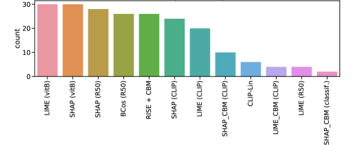
Figure 10: Histogram showing the top-12 XAI techniques preferred by each annotator.

To further explore annotator preferences, we identified the top-12 XAI techniques selected by each annotator and visualized the results in the histogram shown in Figure 10. From this figure, we observe that classical methods such as LIME and SHAP stand out as the most frequently preferred. This suggests a strong preference for well-established saliency-based methods. Additionally, there is a notable inclination towards methods that probe the model’s reaction to input perturbations. A distinct aspect is the inclusion of B-cos, which generates explanations through the incorporation of a dedicated layer, offering a unique mechanism compared to other perturbation-based techniques. Of the 11 most popular techniques among annotators, only four are based on Concept Bottleneck Models (CBMs), indicating a general preference for saliency maps over concept-based explanations. Unlike Table 10, this analysis focuses on the top-12 techniques per annotator, removing the influence of votes among the top-12 techniques to reduce noise and better capture annotator preferences.

Next, we aggregated the scores using majority voting and calculated QWC scores to measure the agreement between individual annotators and the aggregated score. We further analyzed the QWC scores by gender and age groups to assess any systematic differences in interpretation. As shown in Figure 12, the kappa scores indicate that there is generally consistent agreement across different age and sex groups, although older annotators show slightly less consistency. This highlights that while demographic factors may introduce some variation, they do not substantially impact the overall interpretability evaluation.

We also investigated potential biases in the annotations themselves by examining the differences in how annotators approached CBM-based and saliency-based explanations. For CBM explanations, we focused on the text written by annotators in response to question Q0.1, assessing whether annotators preferred explanations that closely resembled their own textual responses. To quantify this, we transformed CBM explanations into text by concatenating the top concepts used in the explanation and calculated the BLEU (Papineni et al., 2002) and ROUGE scores (Lin, 2004) between these explanations and the annotators’ text responses. As shown in Figure 11, the ROUGE score reveals a slight correlation between the explanations and the annotators’ expectations for questions Q1, Q2, Q3, and Q4. This suggests that annotators are inclined to favor explanations that align with their preconceived notions, potentially introducing a bias toward consistency with their initial answers.

Moreover, we observed that questions Q1, Q2, Q3, and Q4 exhibit high intercorrelation, as do questions Q5 and Q6. This clustering indicates that annotators tend to evaluate explanations similarly across these sets of questions, which may reflect underlying patterns in how different types of explanations are perceived.

For saliency-based explanations, we analyzed the bounding boxes provided by annotators in response to question Q0.2. We evaluated the correlation between various metrics and the annotators’ answers, including:

1. the total sum of pixel intensities in the saliency map (“SUM_all”),

2. the sum of pixel intensities within the area of the image identified by the bounding box (“SUM_pos”),

3. the sum of pixel intensities outside the bounding box (“SUM_neg”),

4. the entropy of the saliency map (“Entropy”).

Figure 11 shows that questions Q1, Q2, Q3, and Q4 are highly correlated with each other, as are questions Q5 and Q6. Additionally, all metrics except for “SUM_pos” show some correlation with questions Q1–Q4. This suggests that annotators may focus heavily on background features and salient objects when answering these questions, potentially overlooking finer details in the bounding box area.

Overall, these analyses highlight several potential biases in the dataset. Annotators exhibit a preference for certain types of explanations, particularly saliency maps, and tend to favor explanations that align with their expectations, as evidenced by the correlation between their text responses and the explanations. Additionally, while demographic factors such as age and gender do not significantly impact the overall evaluation, the slight decrease in consistency among older annotators warrants further investigation. The study involved 15 annotators, all from the same cultural background, which may introduce some shared perspectives or biases. To mitigate this, future studies could benefit from a more diverse group of annotators.

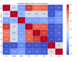
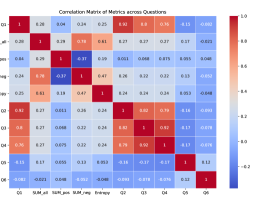
CBM	Saliency map

Figure 11: Correlation between the various questions and key metrics for saliency and CBM explanations. For CBM, the criteria used are the BLEU (Papineni et al., 2002) and ROUGE scores (Lin, 2004) scores between the explanation and the text from question Q0.1. For saliency maps, the metrics include the total pixel sum (SUM_all), the sum of pixels within the annotator-provided bounding box (SUM_pos) from question Q0.2, the sum of pixels outside the bounding box (SUM_neg), and the entropy of the saliency map (Entropy).

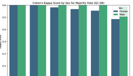
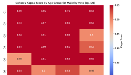
Figure 12: Cohen’s kappa statistics showing agreement between annotators, aggregated by sex and age groups.

B.3 Additional results of the human evaluations

In Table 10, we present the average mode of votes for each XAI technique. the first observation is that it is difficult to observe clear differences among XAI methods. This is mainly due to the fact XAI methods are highly sensible to the backbone they are applied on, as noticed in Section 3.5. We observe also that the average score for saliency-based techniques across fidelity related questions is 2.47, while for CBMs, the average score is lower at 2.12. For saliency-based techniques across complexity related questions is 2.44, while for CBMs, the average score is also lower at 2.10. For saliency-based techniques across objectivity related questions is 2.46, while for CBMs, the average score is also lower at 2.11. For robustness related questions, the average scores are 3.59 for saliency-based techniques and 3.20 for CBMs.

Table 10: XAI techniques with aggregated scores across different evaluation metrics.

	Fidelity	Complexity	Objectivity	Robustness
XAI Technique	(Q1)	(Q2-Q3)	(Q4)	(Q5-Q6)
GradCAM (ResNet50)	2.50	2.53	2.60	3.83
GradCAM (ViT-B)	2.77	2.86	3.00	3.57
GradCAM (CLIP-zero-shot)	1.86	1.78	1.76	3.90
LIME (ResNet50)	2.16	2.08	2.13	4.28
LIME (ViT-B)	3.06	2.98	2.99	3.89
LIME (CLIP-zero-shot)	2.48	2.49	2.51	4.25
SHAP (ResNet50)	2.63	2.66	2.65	3.74
SHAP (ViT-B)	2.87	2.85	2.89	3.64
SHAP (CLIP-zero-shot)	2.55	2.52	2.47	3.70
AblationCAM (ResNet50)	2.78	2.96	2.91	3.14
AblationCAM (ViT-B)	1.75	1.75	1.75	3.84
AblationCAM (CLIP-zero-shot)	1.27	1.34	1.36	3.64
EigenCAM (ResNet50)	2.23	2.23	2.41	3.21
EigenCAM (ViT-B)	3.31	3.25	3.15	3.39
EigenCAM (CLIP-zero-shot)	3.68	3.68	3.64	3.28
EigenGradCAM (ResNet50)	2.81	2.91	3.10	3.24
EigenGradCAM (ViT-B)	1.41	1.21	1.21	3.86
EigenGradCAM (CLIP-zero-shot)	2.29	2.10	2.05	3.67
FullGrad (ResNet50)	3.65	3.68	3.65	3.26
FullGrad (ViT-B)	1.65	1.50	1.65	4.00
GradCAMPlusPlus (ResNet50)	2.55	2.60	2.60	3.45
GradCAMPlusPlus (ViT-B)	2.19	2.00	1.90	3.93
GradCAMPlusPlus (CLIP-zero-shot)	1.80	1.88	1.85	4.13
GradCAMElementWise (ResNet50)	3.04	2.78	2.74	3.59
GradCAMElementWise (ViT-B)	1.47	1.53	1.53	3.90
GradCAMElementWise (CLIP-zero-shot)	2.39	2.33	2.35	3.24
HiResCAM (ResNet50)	2.96	2.77	2.83	3.52
HiResCAM (ViT-B)	1.45	1.30	1.30	4.10
HiResCAM (CLIP-zero-shot)	1.83	1.79	1.92	3.85
ScoreCAM (ResNet50)	2.68	2.55	2.45	3.36
ScoreCAM (ViT-B)	3.00	3.00	3.00	3.63
XGradCAM (ResNet50)	2.57	2.72	2.86	3.50
XGradCAM (ViT-B)	2.00	2.18	2.18	4.02
XGradCAM (CLIP-zero-shot)	2.50	2.31	2.21	4.34
DeepFeatureFactorization (ResNet50)	3.50	3.40	3.33	3.25
DeepFeatureFactorization (ViT-B)	2.46	2.66	2.69	3.45
DeepFeatureFactorization (CLIP-zero-shot)	2.94	2.92	3.22	3.61
BCos (ResNet50-BCos)	2.91	2.84	2.77	3.34
CLIP-QDA-sample	1.71	1.69	1.66	4.04
CLIP-Linear-sample	2.19	2.17	2.27	2.89
LIME_CBM (CLIP-QDA)	2.22	2.20	2.25	4.27
SHAP_CBM (CLIP-QDA)	2.44	2.33	2.29	3.81
LIME_CBM (CBM-classifier-logistic)	1.66	1.66	1.65	3.53
SHAP_CBM (CBM-classifier-logistic)	1.98	2.01	1.94	3.30
Xnesyl-Linear	1.72	1.77	1.77	3.82
RISE (CBM-classifier-logistic)	2.65	2.57	2.62	2.70

B.4 Evaluation Questions

In addition to annotating the samples that comprise the PASTA-dataset, each participant in the study was asked to respond to the following questions:

• Q7: Could you rank the different qualities of the explanation in order of importance? Expectedness, Trustworthy, Complexity, Robustness, Objectivity.

• Q8: Can you please order the different questions from Q1, Q2, Q3, Q4, Q5, and Q6 from the less important to the more important questions to assess the quality of the explanation?

• Q9: Can you please order the different questions from Q1, Q2, Q3, Q4, Q5 and Q6 from the most difficult to the easiest?

The results for Q7 are presented in Table 11. The data indicate that evaluators place a higher value on Trustworthiness and Complexity, while Objectivity is ranked significantly lower. This finding aligns with the work of Liao et al. (2022), which poses a similar question but focuses on a pool of experts.

Table 12 summarizes the results for Q8 and Q9. According to user feedback, Q1 is deemed the most important question. Notably, there is a strong correlation between the responses to Q8 and Q9: the questions perceived as easiest to answer are also regarded as the most important. Interestingly, there is a low correlation between the importance assigned to each question and the axioms they represent, highlighting a distinction between the perception of an axiom and the execution of the associated task. Furthermore, both Q8 and Q9 reveal a separation in ranking among Q1 to Q4 and Q5 and Q6, which resonates with the dataset analysis discussed in Section B.2.

Table 11: Average positions of axioms for question 7. Lower rankings indicate that the axiom is considered more important by evaluators, while higher rankings suggest the axiom is considered less important. Results sorted by ascending order.

Axiom	Average Position (Q7) $\downarrow$
Trustworthy	2.47 $\pm$ 1.48
Complexity	2.53 $\pm$ 1.58
Robustness	2.97 $\pm$ 1.06
Expectedness	3.20 $\pm$ 1.05
Objectivity	3.77 $\pm$ 1.36

Table 12: Average positions of questions 1 to 6 for Q8 and Q9. For Q8, higher rankings indicate that the question is considered more important by evaluators, while lower rankings suggest the question is considered less important. For Q9, lower rankings indicate that the question is considered more difficult to evaluate, while lower rankings suggest the question is considered less difficult.

Question	Average Position (Q8) $\uparrow$	Average Position (Q9) $\downarrow$
Q1	4.10 $\pm$ 1.32	4.00 $\pm$ 1.21
Q2	3.90 $\pm$ 1.29	4.23 $\pm$ 1.35
Q3	4.03 $\pm$ 1.77	4.53 $\pm$ 1.70
Q4	3.13 $\pm$ 1.41	3.67 $\pm$ 1.40
Q5	2.63 $\pm$ 1.66	1.80 $\pm$ 0.57
Q6	3.00 $\pm$ 1.95	2.54 $\pm$ 1.72

Appendix C PASTA-metric

C.1 Implementation details

C.1.1 Aggregation of the votes.

In the dataset, we have access to 5 votes per question. Then, if we denote the set of votes as $\{m_{i}^{j}[a]\}_{a=1}^{N_{a}}$, where $N_{a}=5$ is the number of annotations:

$$\text{Mode}(m_{i}^{j})=\underset{a}{\arg\max}\;\text{Count}(m_{i}^{j}[a])\,,$$ (4)

where $\text{Count}(m_{i}^{j}[a])$ represents the frequency of each vote $a$ in the set.

C.1.2 Evaluation metrics

The quadratic weighted Cohen’s Kappa (QWK) measures inter-rater agreement, adjusting for chance and penalizing disagreement based on its magnitude. The formula is:

$$\text{QWK}=\frac{\sum_{i,j}w_{ij}O_{ij}-\sum_{i,j}w_{ij}E_{ij}}{1-\sum_{i,j}w_{ij}E_{ij}},$$ (5)

where:

• $O_{ij}$ and $E_{ij}$ are the observed and expected frequencies, respectively.

• $w_{ij}=1-\frac{(i-j)^{2}}{(k-1)^{2}}$ is the quadratic weight for categories $i$ and $j$.

The Mean Squared Error (MSE) measures the average squared difference between predicted and actual values. It is given by:

$$\text{MSE}=\frac{1}{N_{s}}\sum_{k=1}^{N_{s}}(m_{k}-\hat{m}_{k})^{2}\,.$$ (6)

The Spearman Correlation Coefficient (SCC) measures the rank correlation between two variables. It is calculated using the ranks of the data points and is given by:

$$\text{SCC}=1-\frac{6\sum_{i}d_{i}^{2}}{N_{s}(N_{s}^{2}-1)},$$ (7)

where $d_{i}$ is the difference between the ranks of each pair of values.

C.2 Ablation studies

C.2.1 Aggregation of the votes

Given the subjective nature of the annotations and the presence of multiple responses to the same question (five answers per question), we explored different methods for determining the ground truth. In Table 13, we tested how PASTA-metric training is affected when using the mean, mode, or median as the ground truth. Since this parameter significantly impacts the dispersion of the samples, it is not surprising that the results vary, particularly when using the mean. However, in all our experiments, we opted to use the mode, as phenomena of high non-consensus were observed (see Appendix B.2).

Table 13: Comparison of the influence of ground truth generation methods. Each value is the average result on 5 runs with the standard deviation.

Label Type	MSE	QWK	SCC
Mean	0.51 $\pm$ 0.03	0.53 $\pm$ 0.04	0.27 $\pm$ 0.27
Mode	0.84 $\pm$ 0.06	0.56 $\pm$ 0.05	0.28 $\pm$ 0.29
Median	0.73 $\pm$ 0.06	0.55 $\pm$ 0.06	0.28 $\pm$ 0.28

C.2.2 Losses

C.3 Loss Functions

Here we define the tree losses used to train our PASTA-model.

The Cosine Similarity Loss measures the cosine similarity between the predicted explanations $\hat{m}_{k}$ and the ground truth explanations $m_{k}$, ensuring alignment in their direction:

$$L_{s}=1-\frac{\sum_{k=1}^{N_{s}}\hat{m}_{k}m_{k}}{\sqrt{\sum_{k=1}^{N_{s}}\hat{m}_{k}^{2}}\sqrt{\sum_{k=1}^{N_{s}}m_{k}^{2}}}$$ (8)

The Mean Squared Error (MSE) loss measures the squared difference between predicted and true explanations, penalizing larger errors more heavily:

$$L_{mse}=\frac{1}{N_{s}}\sum_{k=1}^{N_{s}}(\hat{m}_{k}-m_{k})^{2}$$ (9)

This Ranking Loss ensures the correct ranking of explanations by penalizing cases where the predicted ranking contradicts the true ranking:

$$L_{r}=\frac{1}{\hat{N_{s}}}\sum_{k_{1},k_{2}}\max(0,-(\hat{m}_{k_{1}}-\hat{m}_{k_{2}})(m_{k_{1}}-m_{k_{2}}))$$ (10)

Here, $\hat{N_{s}}$ represents the total number of pairs considered for the ranking loss.

C.3.1 Explanation embeddings

Saliency

Regarding saliency-based explanations, a key question arises about what should be considered as the image representing the explanation. Two variants were considered: using the heatmap visualization that is presented to users, as shown in Equation 1, or the input image as defined as:

$$\phi_{\text{image}}({\bm{e}}_{i}^{j})=\text{CLIP}_{\text{image}}({\bm{x}}_{i}\times{\bm{e}}_{i}^{j})$$ (11)

The element-wise multiplication of the input image with the saliency map selectively blurs the image, with regions corresponding to lower activation values being blurred, while areas with higher activation values remain clear.

The results are presented in Table 14, where a slight improvement is observed in favor of using the image as a heatmap. This can be attributed to the fact that, despite being more computationally ambiguous, the heatmap display reveals the entire image. Additionally, this representation closely resembles the format of the samples provided to annotators.

Table 14: Influence of the saliency computation process. Heatmap refers to the process defined in Equation 1 and Masked image refers to the process defined in Equation 11. Each value is the average result on 5 runs with the standard deviation.

Embedded Image	MSE	QWK	SCC
Heatmap	0.85 $\pm$ 0.06	0.55 $\pm$ 0.04	0.28 $\pm$ 0.28
Masked image	0.89 $\pm$ 0.09	0.54 $\pm$ 0.05	0.27 $\pm$ 0.28

CBM

Concerning concept bottleneck explanation, which basically can be interpreted as a dictionary attributing a scalar for each concept. One crucial step is converting CBM activations to CLIP embeddings. We tested two ways do do so:

• By considering the raw text of concepts, ordered by importance (Equation 2)

• By using a sum of all the CLIP embeddings of text, weightened by its activations:

  $$\phi_{text}({\bm{e}}_{i}^{j})=\frac{1}{||{\bm{e}}_{i}^{j}||}\sum_{k}^{N_{k}}{\bm{e}}_{i}^{j}[k]~{}CLIP_{text}(concept_{i}[k])$$ (12)

If we use the first solution, there is questions about the number of concepts to keep, that we note as the parameters $N_{top}$. Table 15 presents the influence of $N_{top}$ while 16 presents the influence of diffetents ways to compute the embedings.

Table 15: Influence of the number of words selected as an input text $N_{top}$. Each value is the average result on 5 runs with the standard deviation.

$N_{top}$	MSE	QWK	SCC
5	0.86 $\pm$ 0.06	0.53 $\pm$ 0.06	0.27 $\pm$ 0.27
10	0.87 $\pm$ 0.04	0.54 $\pm$ 0.05	0.27 $\pm$ 0.27
15	0.89 $\pm$ 0.05	0.54 $\pm$ 0.03	0.27 $\pm$ 0.27
20	0.85 $\pm$ 0.06	0.55 $\pm$ 0.04	0.28 $\pm$ 0.28
25	0.84 $\pm$ 0.05	0.54 $\pm$ 0.03	0.28 $\pm$ 0.28
30	0.85 $\pm$ 0.06	0.53 $\pm$ 0.05	0.27 $\pm$ 0.27

Table 16: Influence of the CBM explanation embedding process. Weightened refers to the process described in Equation 12, Sentence refers to the process described in Equation 2, preceded with the template noted in Template. Each value is the average result on 5 runs with the standard deviation.

Computation	MSE	QWK	SCC	Template
Weightened	0.86 $\pm$ 0.06	0.53 $\pm$ 0.05	0.27 $\pm$ 0.28	–
Sentence	0.85 $\pm$ 0.06	0.55 $\pm$ 0.04	0.28 $\pm$ 0.28	“ ”
Sentence	0.82 $\pm$ 0.08	0.54 $\pm$ 0.06	0.27 $\pm$ 0.28	“The model’s prediction is motivated by the concepts: ”

References

- Agarwal et al. (2022a) Chirag Agarwal, Nari Johnson, Martin Pawelczyk, Satyapriya Krishna, Eshika Saxena, Marinka Zitnik, and Himabindu Lakkaraju. Rethinking stability for attribution-based explanations. arXiv preprint arXiv:2203.06877, 2022a.
- Agarwal et al. (2022b) Chirag Agarwal, Satyapriya Krishna, Eshika Saxena, Martin Pawelczyk, Nari Johnson, Isha Puri, Marinka Zitnik, and Himabindu Lakkaraju. Openxai: Towards a transparent evaluation of model explanations. Advances in Neural Information Processing Systems, 35:15784–15799, 2022b.
- Alvarez-Melis & Jaakkola (2018a) David Alvarez-Melis and Tommi Jaakkola. Towards robust interpretability with self-explaining neural networks. Advances in Neural Information Processing Systems, 31, 2018a.
- Alvarez-Melis & Jaakkola (2018b) David Alvarez-Melis and Tommi S. Jaakkola. On the robustness of interpretability methods. arXiv preprint arXiv:1806.08049, 2018b.
- Ancona et al. (2017) Marco Ancona, Enea Ceolini, Cengiz Öztireli, and Markus Gross. Towards better understanding of gradient-based attribution methods for deep neural networks. arXiv preprint arXiv:1711.06104, 2017.
- Arrieta et al. (2020) Alejandro Barredo Arrieta, Natalia Díaz-Rodríguez, Javier Del Ser, Adrien Bennetot, Siham Tabik, Alberto Barbado, Salvador García, Sergio Gil-López, Daniel Molina, Richard Benjamins, et al. Explainable artificial intelligence (XAI): Concepts, taxonomies, opportunities and challenges toward responsible ai. Information Fusion, 58:82–115, 2020.
- Arya et al. (2019) Vijay Arya, Rachel K.E. Bellamy, Pin-Yu Chen, Amit Dhurandhar, Michael Hind, Samuel C. Hoffman, Stephanie Houde, Q. Vera Liao, Ronny Luss, Aleksandra Mojsilović, et al. One explanation does not fit all: A toolkit and taxonomy of ai explainability techniques. arXiv preprint arXiv:1909.03012, 2019.
- Augustin et al. (2022) Maximilian Augustin, Valentyn Boreiko, Francesco Croce, and Matthias Hein. Diffusion visual counterfactual explanations. Advances in Neural Information Processing Systems, 35:364–377, 2022.
- Azzolin et al. (2024) Steve Azzolin, Antonio Longa, Stefano Teso, and Andrea Passerini. Perks and pitfalls of faithfulness in regular, self-explainable and domain invariant GNNs. arXiv preprint arXiv:2406.15156, 2024.
- Bach et al. (2015) Sebastian Bach, Alexander Binder, Grégoire Montavon, Frederick Klauschen, Klaus-Robert Müller, and Wojciech Samek. On pixel-wise explanations for non-linear classifier decisions by layer-wise relevance propagation. PloS One, 10(7):e0130140, 2015.
- Bénard et al. (2021) Clément Bénard, Gérard Biau, Sébastien Da Veiga, and Erwan Scornet. Interpretable random forests via rule extraction. In International Conference on Artificial Intelligence and Statistics, pp. 937–945, 2021.
- Bender et al. (2021) Emily M Bender, Timnit Gebru, Angelina McMillan-Major, and Shmargaret Shmitchell. On the dangers of stochastic parrots: Can language models be too big? In Proceedings of the 2021 ACM conference on fairness, accountability, and transparency, pp. 610–623, 2021.
- Bennetot et al. (2022) Adrien Bennetot, Gianni Franchi, Javier Del Ser, Raja Chatila, and Natalia Diaz-Rodriguez. Greybox XAI: A neural-symbolic learning framework to produce interpretable predictions for image classification. Knowledge-Based Systems, 258:109947, 2022.
- Bhatt et al. (2021) Umang Bhatt, Adrian Weller, and José M. F. Moura. Evaluating and aggregating feature-based model explanations. In Proceedings of the Twenty-Ninth International Joint Conference on Artificial Intelligence, IJCAI’20, 2021.
- Biessmann & Refiano (2021) Felix Biessmann and Dionysius Refiano. Quality metrics for transparent machine learning with and without humans in the loop are not correlated. arXiv preprint arXiv:2107.02033, 2021.
- Böhle et al. (2024) Moritz Böhle, Navdeeppal Singh, Mario Fritz, and Bernt Schiele. B-cos alignment for inherently interpretable CNNs and vision transformers. IEEE Transactions on Pattern Analysis and Machine Intelligence, 2024.
- Castelvecchi (2016) Davide Castelvecchi. Can we open the black box of AI? Nature News, 538(7623):20, 2016.
- Chalasani et al. (2020) Prasad Chalasani, Jiefeng Chen, Amrita Roy Chowdhury, Xi Wu, and Somesh Jha. Concise explanations of neural networks using adversarial training. In International Conference on Machine Learning, pp. 1383–1391, 2020.
- Chattopadhay et al. (2018) Aditya Chattopadhay, Anirban Sarkar, Prantik Howlader, and Vineeth N. Balasubramanian. Grad-cam++: Generalized gradient-based visual explanations for deep convolutional networks. In 2018 IEEE Winter Conference on Applications of Computer Vision (WACV), pp. 839–847. IEEE, 2018.
- Chen et al. (2018) Chong Chen, Min Zhang, Yiqun Liu, and Shaoping Ma. Neural attentional rating regression with review-level explanations. In Proceedings of the 2018 World Wide Web Conference, pp. 1583–1592, 2018.
- Chen et al. (2014) Xianjie Chen, Roozbeh Mottaghi, Xiaobai Liu, Sanja Fidler, Raquel Urtasun, and Alan Yuille. Detect what you can: Detecting and representing objects using holistic models and body parts. In Proceedings of the IEEE Conference on Computer Vision and Pattern Recognition, pp. 1971–1978, 2014.
- Chiang et al. (2024) Wei-Lin Chiang, Lianmin Zheng, Ying Sheng, Anastasios Nikolas Angelopoulos, Tianle Li, Dacheng Li, Hao Zhang, Banghua Zhu, Michael Jordan, Joseph E. Gonzalez, and Ion Stoica. Chatbot arena: An open platform for evaluating LLMs by human preference, 2024.
- Colin et al. (2022) Julien Colin, Thomas Fel, Rémi Cadène, and Thomas Serre. What I cannot predict, I do not understand: A human-centered evaluation framework for explainability methods. Advances in Neural Information Processing Systems, 35:2832–2845, 2022.
- Collins et al. (2018) Edo Collins, Radhakrishna Achanta, and Sabine Susstrunk. Deep feature factorization for concept discovery. In Proceedings of the European Conference on Computer Vision (ECCV), pp. 336–352, 2018.
- Cowan (2001) Nelson Cowan. The magical number 4 in short-term memory: A reconsideration of mental storage capacity. Behavioral and Brain Sciences, 24(1):87–114, 2001.
- Dasgupta et al. (2022) Sanjoy Dasgupta, Nave Frost, and Michal Moshkovitz. Framework for evaluating faithfulness of local explanations. In International Conference on Machine Learning, pp. 4794–4815, 2022.
- Dawoud et al. (2023) Karam Dawoud, Wojciech Samek, Peter Eisert, Sebastian Lapuschkin, and Sebastian Bosse. Human-centered evaluation of XAI methods. In 2023 IEEE International Conference on Data Mining Workshops (ICDMW), pp. 912–921. IEEE, 2023.
- DeYoung et al. (2020) Jay DeYoung, Sarthak Jain, Nazneen Fatema Rajani, Eric Lehman, Caiming Xiong, Richard Socher, and Byron C. Wallace. Eraser: A benchmark to evaluate rationalized NLP models. In Proceedings of the 58th Annual Meeting of the Association for Computational Linguistics, pp. 4443–4458, 2020.
- Díaz-Rodríguez et al. (2022) Natalia Díaz-Rodríguez, Alberto Lamas, Jules Sanchez, Gianni Franchi, Ivan Donadello, Siham Tabik, David Filliat, Policarpo Cruz, Rosana Montes, and Francisco Herrera. Explainable neural-symbolic learning (x-nesyl) methodology to fuse deep learning representations with expert knowledge graphs: The monumai cultural heritage use case. Information Fusion, 79:58–83, 2022.
- Doshi-Velez & Kim (2017) Finale Doshi-Velez and Been Kim. Towards a rigorous science of interpretable machine learning. arXiv preprint arXiv:1702.08608, 2017.
- Dosovitskiy (2020) Alexey Dosovitskiy. An image is worth 16x16 words: Transformers for image recognition at scale. arXiv preprint arXiv:2010.11929, 2020.
- Draelos & Carin (2020) Rachel Lea Draelos and Lawrence Carin. Use hirescam instead of grad-cam for faithful explanations of convolutional neural networks. arXiv preprint arXiv:2011.08891, 2020.
- Fel et al. (2022a) Thomas Fel, Lucas Hervier, David Vigouroux, Antonin Poche, Justin Plakoo, Remi Cadene, Mathieu Chalvidal, Julien Colin, Thibaut Boissin, Louis Bethune, Agustin Picard, Claire Nicodeme, Laurent Gardes, Gregory Flandin, and Thomas Serre. Xplique: A deep learning explainability toolbox. Workshop on Explainable Artificial Intelligence for Computer Vision (CVPR), 2022a.
- Fel et al. (2022b) Thomas Fel, David Vigouroux, Rémi Cadène, and Thomas Serre. How good is your explanation? algorithmic stability measures to assess the quality of explanations for deep neural networks. In Proceedings of the IEEE/CVF Winter Conference on Applications of Computer Vision, pp. 720–730, 2022b.
- Fowler Jr (2013) Floyd J. Fowler Jr. Survey Research Methods. Sage Publications, 2013.
- Fu et al. (2020) Ruigang Fu, Qingyong Hu, Xiaohu Dong, Yulan Guo, Yinghui Gao, and Biao Li. Axiom-based grad-cam: Towards accurate visualization and explanation of CNNs. arXiv preprint arXiv:2008.02312, 2020.
- Ge et al. (2023) Jiaxin Ge, Hongyin Luo, Siyuan Qian, Yulu Gan, Jie Fu, and Shanghang Zhang. Chain of thought prompt tuning in vision language models. arXiv preprint arXiv:2304.07919, 2023.
- Gunning et al. (2019) David Gunning, Mark Stefik, Jaesik Choi, Timothy Miller, Simone Stumpf, and Guang-Zhong Yang. Xai—explainable artificial intelligence. Science Robotics, 4(37):eaay7120, 2019.
- Hase et al. (2024) Peter Hase, Harry Xie, and Mohit Bansal. The out-of-distribution problem in explainability and search methods for feature importance explanations. In Proceedings of the 35th International Conference on Neural Information Processing Systems, 2024.
- He et al. (2016) Kaiming He, Xiangyu Zhang, Shaoqing Ren, and Jian Sun. Deep residual learning for image recognition. In Proceedings of the IEEE conference on computer vision and pattern recognition, pp. 770–778, 2016.
- Hedström et al. (2023) Anna Hedström, Leander Weber, Daniel Krakowczyk, Dilyara Bareeva, Franz Motzkus, Wojciech Samek, Sebastian Lapuschkin, and Marina Marina M.-C. Höhne. Quantus: An explainable AI toolkit for responsible evaluation of neural network explanations and beyond. Journal of Machine Learning Research, 24(34):1–11, 2023.
- Hurley & Rickard (2009) Niall Hurley and Scott Rickard. Comparing measures of sparsity. IEEE Transactions on Information Theory, 55(10):4723–4741, 2009.
- Jiang et al. (2021) Peng-Tao Jiang, Chang-Bin Zhang, Qibin Hou, Ming-Ming Cheng, and Yunchao Wei. Layercam: Exploring hierarchical class activation maps for localization. IEEE Transactions on Image Processing, 30:5875–5888, 2021.
- Kaufmann et al. (2023) Timo Kaufmann, Paul Weng, Viktor Bengs, and Eyke Hüllermeier. A survey of reinforcement learning from human feedback. arXiv preprint arXiv:2312.14925, 2023.
- Kazmierczak et al. (2024) Rémi Kazmierczak, Eloïse Berthier, Goran Frehse, and Gianni Franchi. CLIP-QDA: An explainable concept bottleneck model. Transactions on Machine Learning Research Journal, 2024.
- Koh et al. (2020) Pang Wei Koh, Thao Nguyen, Yew Siang Tang, Stephen Mussmann, Emma Pierson, Been Kim, and Percy Liang. Concept bottleneck models. In International Conference on Machine Learning, pp. 5338–5348, 2020.
- Lamas et al. (2021) Alberto Lamas, Siham Tabik, Policarpo Cruz, Rosana Montes, Álvaro Martinez-Sevilla, Teresa Cruz, and Francisco Herrera. Monumai: Dataset, deep learning pipeline and citizen science based app for monumental heritage taxonomy and classification. Neurocomputing, 420:266–280, 2021.
- Lee et al. (2024) Seongyun Lee, Seungone Kim, Sue Hyun Park, Geewook Kim, and Minjoon Seo. Prometheusvision: Vision-language model as a judge for fine-grained evaluation. arXiv preprint arXiv:2401.06591, 2024.
- Li et al. (2023a) Feng Li, Xuefeng Xi, Zhiming Cui, Dongyang Li, and Wanting Zeng. Automatic essay scoring method based on multi-scale features. Applied Sciences, 13(11):6775, 2023a.
- Li et al. (2023b) Xuhong Li, Mengnan Du, Jiamin Chen, Yekun Chai, Himabindu Lakkaraju, and Haoyi Xiong. M4: A unified XAI benchmark for faithfulness evaluation of feature attribution methods across metrics, modalities and models. Advances in Neural Information Processing Systems, 36:1630–1643, 2023b.
- Liao et al. (2022) Q. Vera Liao, Yunfeng Zhang, Ronny Luss, Finale Doshi-Velez, and Amit Dhurandhar. Connecting algorithmic research and usage contexts: a perspective of contextualized evaluation for explainable AI. In Proceedings of the AAAI Conference on Human Computation and Crowdsourcing, volume 10, pp. 147–159, 2022.
- Lin (2004) Chin-Yew Lin. Rouge: A package for automatic evaluation of summaries. In Text summarization branches out, pp. 74–81, 2004.
- Lin et al. (2014) Tsung-Yi Lin, Michael Maire, Serge Belongie, James Hays, Pietro Perona, Deva Ramanan, Piotr Dollár, and C. Lawrence Zitnick. Microsoft COCO: Common objects in context. In Computer Vision–ECCV 2014: 13th European Conference, Zurich, Switzerland, September 6-12, 2014, Proceedings, Part V 13, pp. 740–755. Springer, 2014.
- Litjens et al. (2017) Geert Litjens, Thijs Kooi, Babak Ehteshami Bejnordi, Arnaud Arindra Adiyoso Setio, Francesco Ciompi, Mohsen Ghafoorian, Jeroen Awm Van Der Laak, Bram Van Ginneken, and Clara I. Sánchez. A survey on deep learning in medical image analysis. Medical Image Analysis, 42:60–88, 2017.
- Liu et al. (2023) Shilong Liu, Zhaoyang Zeng, Tianhe Ren, Feng Li, Hao Zhang, Jie Yang, Chunyuan Li, Jianwei Yang, Hang Su, Jun Zhu, et al. Grounding dino: Marrying dino with grounded pre-training for open-set object detection. arXiv preprint arXiv:2303.05499, 2023.
- Lopes et al. (2022) Pedro Lopes, Eduardo Silva, Cristiana Braga, Tiago Oliveira, and Luís Rosado. XAI systems evaluation: A review of human and computer-centred methods. Applied Sciences, 12(19):9423, 2022.
- Lundberg & Lee (2017) Scott M. Lundberg and Su-In Lee. A unified approach to interpreting model predictions. Advances in Neural Information Processing Systems, 30, 2017.
- Miró-Nicolau et al. (2022) Miquel Miró-Nicolau, Gabriel Moyà-Alcover, and Antoni Jaume-i Capó. Evaluating explainable artificial intelligence for x-ray image analysis. Applied Sciences, 12(9):4459, 2022.
- Mohseni et al. (2021) Sina Mohseni, Jeremy E. Block, and Eric Ragan. Quantitative evaluation of machine learning explanations: A human-grounded benchmark. In 26th International Conference on Intelligent User Interfaces, pp. 22–31, 2021.
- Montavon et al. (2018) Grégoire Montavon, Wojciech Samek, and Klaus-Robert Müller. Methods for interpreting and understanding deep neural networks. Digital Signal Processing, 73:1–15, 2018.
- Muddamsetty et al. (2021) Satya M. Muddamsetty, Mohammad N.S. Jahromi, and Thomas B. Moeslund. Expert level evaluations for explainable AI (XAI) methods in the medical domain. In International Conference on Pattern Recognition, pp. 35–46. Springer, 2021.
- Muhammad & Yeasin (2020) Mohammed Bany Muhammad and Mohammed Yeasin. Eigen-cam: Class activation map using principal components. In 2020 International Joint Conference on Neural Networks (IJCNN), pp. 1–7. IEEE, 2020.
- Nauta et al. (2023) Meike Nauta, Jan Trienes, Shreyasi Pathak, Elisa Nguyen, Michelle Peters, Yasmin Schmitt, Jörg Schlötterer, Maurice van Keulen, and Christin Seifert. From anecdotal evidence to quantitative evaluation methods: A systematic review on evaluating explainable AI. ACM Computing Surveys, 55(13s):1–42, 2023.
- Nguyen & Martínez (2020) An-phi Nguyen and María Rodríguez Martínez. On quantitative aspects of model interpretability. arXiv preprint arXiv:2007.07584, 2020.
- Papineni et al. (2002) Kishore Papineni, Salim Roukos, Todd Ward, and Wei-Jing Zhu. Bleu: a method for automatic evaluation of machine translation. In Proceedings of the 40th annual meeting of the Association for Computational Linguistics, pp. 311–318, 2002.
- Petsiuk et al. (2018) Vitali Petsiuk, Abir Das, and Kate Saenko. Rise: Randomized input sampling for explanation of black-box models. arXiv preprint arXiv:1806.07421, 2018.
- Pillai & Pirsiavash (2021) Vipin Pillai and Hamed Pirsiavash. Explainable models with consistent interpretations. In Proceedings of the AAAI Conference on Artificial Intelligence, volume 35, pp. 2431–2439, 2021.
- Pommeranz et al. (2012) Alina Pommeranz, Joost Broekens, Pascal Wiggers, Willem-Paul Brinkman, and Catholijn M. Jonker. Designing interfaces for explicit preference elicitation: a user-centered investigation of preference representation and elicitation process. User Modeling and User-Adapted Interaction, 22:357–397, 2012.
- Radford et al. (2021) Alec Radford, Jong Wook Kim, Chris Hallacy, Aditya Ramesh, Gabriel Goh, Sandhini Agarwal, Girish Sastry, Amanda Askell, Pamela Mishkin, Jack Clark, et al. Learning transferable visual models from natural language supervision. In International Conference on Machine Learning, pp. 8748–8763, 2021.
- Ramaswamy et al. (2020) Harish Guruprasad Ramaswamy et al. Ablation-cam: Visual explanations for deep convolutional network via gradient-free localization. In Proceedings of the IEEE/CVF Winter Conference on Applications of Computer Vision, pp. 983–991, 2020.
- Rathee et al. (2022) Mandeep Rathee, Thorben Funke, Avishek Anand, and Megha Khosla. Bagel: A benchmark for assessing graph neural network explanations. arXiv preprint arXiv:2206.13983, 2022.
- Ribeiro et al. (2016) Marco Tulio Ribeiro, Sameer Singh, and Carlos Guestrin. “Why should I trust you?”: Explaining the predictions of any classifier. In Proceedings of the 22nd ACM SIGKDD International Conference on Knowledge Discovery and Data Mining, San Francisco, CA, USA, August 13-17, 2016, pp. 1135–1144, 2016.
- Rieger & Hansen (2020) Laura Rieger and Lars Kai Hansen. Irof: a low resource evaluation metric for explanation methods. arXiv preprint arXiv:2003.08747, 2020.
- Rong et al. (2022) Yao Rong, Tobias Leemann, Vadim Borisov, Gjergji Kasneci, and Enkelejda Kasneci. A consistent and efficient evaluation strategy for attribution methods. arXiv preprint arXiv:2202.00449, 2022.
- Roy et al. (2022) Saumendu Roy, Gabriel Laberge, Banani Roy, Foutse Khomh, Amin Nikanjam, and Saikat Mondal. Why don’t XAI techniques agree? characterizing the disagreements between post-hoc explanations of defect predictions. In 2022 IEEE International Conference on Software Maintenance and Evolution (ICSME), pp. 444–448. IEEE, 2022.
- Rudin et al. (2022) Cynthia Rudin, Chaofan Chen, Zhi Chen, Haiyang Huang, Lesia Semenova, and Chudi Zhong. Interpretable machine learning: Fundamental principles and 10 grand challenges. Statistic Surveys, 16:1–85, 2022.
- Samek et al. (2016) Wojciech Samek, Alexander Binder, Grégoire Montavon, Sebastian Lapuschkin, and Klaus-Robert Müller. Evaluating the visualization of what a deep neural network has learned. IEEE Transactions on Neural Networks and Learning Systems, 28(11):2660–2673, 2016.
- Schmidt et al. (2007) Christina Schmidt, Fabienne Collette, Christian Cajochen, and Philippe Peigneux. A time to think: circadian rhythms in human cognition. Cognitive neuropsychology, 24(7):755–789, 2007.
- Selvaraju et al. (2017) Ramprasaath R. Selvaraju, Michael Cogswell, Abhishek Das, Ramakrishna Vedantam, Devi Parikh, and Dhruv Batra. Grad-cam: Visual explanations from deep networks via gradient-based localization. In Proceedings of the IEEE International Conference on Computer Vision, pp. 618–626, 2017.
- Shu et al. (2019) Kai Shu, Limeng Cui, Suhang Wang, Dongwon Lee, and Huan Liu. defend: Explainable fake news detection. In Proceedings of the 25th ACM SIGKDD International Conference on Knowledge Discovery & Data Mining, pp. 395–405, 2019.
- Srinivas & Fleuret (2019) Suraj Srinivas and François Fleuret. Full-gradient representation for neural network visualization. Advances in Neural Information Processing Systems, 32, 2019.
- Surden (2021) Harry Surden. Machine learning and law: An overview. Research Handbook on Big Data Law, pp. 171–184, 2021.
- Taghipour & Ng (2016) Kaveh Taghipour and Hwee Tou Ng. A neural approach to automated essay scoring. In Proceedings of the 2016 Conference on Empirical Methods in Natural Language Processing, pp. 1882–1891, 2016.
- Vereschak et al. (2024) Oleksandra Vereschak, Fatemeh Alizadeh, Gilles Bailly, and Baptiste Caramiaux. Trust in AI-assisted decision making: Perspectives from those behind the system and those for whom the decision is made. In Proceedings of the CHI Conference on Human Factors in Computing Systems, pp. 1–14, 2024.
- Wang et al. (2020) Haofan Wang, Zifan Wang, Mengnan Du, Fan Yang, Zijian Zhang, Sirui Ding, Piotr Mardziel, and Xia Hu. Score-cam: Score-weighted visual explanations for convolutional neural networks. In Proceedings of the IEEE/CVF Conference on Computer Vision and Pattern Recognition Workshops, pp. 24–25, 2020.
- Wang et al. (2022a) Lijie Wang, Yaozong Shen, Shuyuan Peng, Shuai Zhang, Xinyan Xiao, Hao Liu, Hongxuan Tang, Ying Chen, Hua Wu, and Haifeng Wang. A fine-grained interpretability evaluation benchmark for neural NLP. In Proceedings of the 26th Conference on Computational Natural Language Learning (CoNLL), pp. 70–84, 2022a.
- Wang et al. (2022b) Yongjie Wang, Chuan Wang, Ruobing Li, and Hui Lin. On the use of BERT for automated essay scoring: Joint learning of multi-scale essay representation. arXiv preprint arXiv:2205.03835, 2022b.
- Xiao et al. (2024) Changrong Xiao, Wenxing Ma, Sean Xin Xu, Kunpeng Zhang, Yufang Wang, and Qi Fu. From automation to augmentation: Large language models elevating essay scoring landscape. arXiv preprint arXiv:2401.06431, 2024.
- Yan et al. (2023) An Yan, Yu Wang, Yiwu Zhong, Chengyu Dong, Zexue He, Yujie Lu, William Yang Wang, Jingbo Shang, and Julian McAuley. Learning concise and descriptive attributes for visual recognition. In Proceedings of the IEEE/CVF International Conference on Computer Vision, pp. 3090–3100, 2023.
- Yang et al. (2020) Ruosong Yang, Jiannong Cao, Zhiyuan Wen, Youzheng Wu, and Xiaodong He. Enhancing automated essay scoring performance via fine-tuning pre-trained language models with combination of regression and ranking. In Findings of the Association for Computational Linguistics: EMNLP 2020, pp. 1560–1569, 2020.
- Yang et al. (2023) Yue Yang, Artemis Panagopoulou, Shenghao Zhou, Daniel Jin, Chris Callison-Burch, and Mark Yatskar. Language in a bottle: Language model guided concept bottlenecks for interpretable image classification. In Proceedings of the IEEE/CVF Conference on Computer Vision and Pattern Recognition, pp. 19187–19197, 2023.
- Yannakoudakis et al. (2011) Helen Yannakoudakis, Ted Briscoe, and Ben Medlock. A new dataset and method for automatically grading esol texts. In Proceedings of the 49th Annual Meeting of the Association for Computational Linguistics: Human Language Technologies, pp. 180–189, 2011.
- Yeh et al. (2019) Chih-Kuan Yeh, Cheng-Yu Hsieh, Arun Suggala, David I. Inouye, and Pradeep K. Ravikumar. On the (in) fidelity and sensitivity of explanations. Advances in Neural Information Processing Systems, 32, 2019.
- Yuksekgonul et al. (2022) Mert Yuksekgonul, Maggie Wang, and James Zou. Post-hoc concept bottleneck models. arXiv preprint arXiv:2205.15480, 2022.
1