See it, Think it, Sorted: Large Multimodal Models are Few-shot Time Series Anomaly Analyzers

Abstract.

Time series anomaly detection (TSAD) is becoming increasingly vital due to the rapid growth of time series data across various sectors. Anomalies in web service data, for example, can signal critical incidents such as system failures or server malfunctions, necessitating timely detection and response. However, most existing TSAD methodologies rely heavily on manual feature engineering or require extensive labeled training data, while also offering limited interpretability. To address these challenges, we introduce a pioneering framework called the Time series Anomaly Multimodal Analyzer (TAMA), which leverages the power of Large Multimodal Models (LMMs) to enhance both the detection and interpretation of anomalies in time series data. By converting time series into visual formats that LMMs can efficiently process, TAMA leverages few-shot in-context learning capabilities to reduce dependence on extensive labeled datasets. Our methodology is validated through rigorous experimentation on multiple real-world datasets, where TAMA consistently outperforms state-of-the-art methods in TSAD tasks. Additionally, TAMA provides rich, natural language-based semantic analysis, offering deeper insights into the nature of detected anomalies. Furthermore, we contribute one of the first open-source datasets that includes anomaly detection labels, anomaly type labels, and contextual descriptions—facilitating broader exploration and advancement within this critical field. Ultimately, TAMA not only excels in anomaly detection but also provide a comprehensive approach for understanding the underlying causes of anomalies, pushing TSAD forward through innovative methodologies and insights.

1. Introduction

Web services have undergone significant expansion and advancement in recent years (Bouasker et al., 2020; Yuan et al., 2022). This expansion has led to the generation of vast amounts of time series data, including key performance indicators (KPIs) from cloud center and wireless base stations (Xu et al., 2018; Yu et al., 2024). Anomalies—defined as unexpected deviations from typical patterns in this data—can signal critical events such as device malfunctions and system failures. Consequently, time series anomaly detection (TSAD) techniques for web services have attracted considerable attention (Chen et al., 2024; Nam et al., 2024), demonstrating significant practical value in monitoring web systems and ensuring service quality. Despite the advancements in TSAD methodologies, existing approaches often struggle with several key challenges.

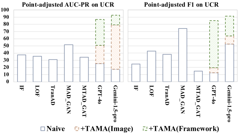
Figure 1. Comparison of AUC-PR and F1 with PA on the UCR dataset. Models include the machine learning (IF, LOF), the deep learning (TranAD, MAD_GAN, MTAD_GAT), and LMMs  (GPT-4o, Gemini-1.5-pro)

Firstly, different methods specialize in different datasets (Zamanzadeh Darban et al., 2024; Rewicki et al., 2023), and an ”one-size-fits-all” universal solution is missing in the filed of TSAD (Schmidl et al., 2022). Diverse approaches in TSAD demonstrate ongoing advancements, each contributing unique methodologies to tackle the inherent challenges of this field. Classical machine learning (ML) methods (Liu et al., 2008; Feng et al., 2019; Ramaswamy et al., 2000; Yairi et al., 2001; Chen and Guestrin, 2016; Huang et al., 2013) are frequently based on strong assumptions or require empirically crafted manual features (Usmani et al., 2022). In contrast, deep learning  (DL) techniques are heavily reliant on hyper-parameters and are either supervised or semi-supervised (Liu et al., 2023; Chalapathy and Chawla, 2019; Pang et al., 2022), necessitating normal data for training— except for (Audibert et al., 2020; Zong et al., 2018; Xu et al., 2018) where other forms of training are required. Noticing that for most real-world datasets, assumptions needed by ML techniques usually do not hold, and training data without anomaly for DL methods are often undesirable, rare, or even unavailable.

Secondly, most existing techniques offer insufficient interpretability, providing a limited understanding of the reasons behind how the anomalies are identified (Jacob et al., 2021). Recently, more works have discussed and attempted to improve the explainability of TSAD algorithms (Jacob et al., 2021; Lee et al., 2023), which is also considered a critical disadvantage of most deep learning methods. Toward this topic, the taxonomy of anomalies has been often mentioned in previous works (Blázquez-García et al., 2021; Choi et al., 2021), where anomalies are categorized into two general types (point and pattern) and several fertilized types (Lai et al., 2021). However, due to the lack of high quality classification labels, few studies have achieved the semantic classification of anomalous data (Kiersztyn et al., 2022; Pang et al., 2022).

Large language models  (LLMs) have revolutionized natural language processing by demonstrating extraordinary capabilities in generalizing across numerous tasks (Naveed et al., 2023; Min et al., 2023). LLMs can function as few-shot or even zero-shot learners (Brown et al., 2020; Gruver et al., 2024), which effectively mitigates the challenge of limited availability of anomaly-free training datasets in TSAD. While LLMs are suitable for solving general problems, there have been attempts to apply them to time series analysis (Jin et al., 2023; Su et al., 2024; Gruver et al., 2024), particularly for forecasting tasks, by trivially feed time series data into LLMs as text (Liu et al., 2024). However, studies have shown that LLMs without fine-tuning fail to achieve comparable results to existing task-specific approaches in time series tasks (Merrill et al., 2024), especially TSAD (Elhafsi et al., 2023; Alnegheimish et al., 2024). One interpretation for this is that LLMs are trained on text data and are insensitive to numerical values (Qian et al., 2022; Ye et al., 2024), making them inherently unsuitable for capturing anomalies with small changes in amplitude (Choi et al., 2021).

To overcome the limitations of LLMs in handling numerical time series data, we introduce an innovative approach: first converting time series into images (“see it”), then utilizing Large Multimodal Models (LMMs) to analyze the visualized time series (“think it”), and finally detecting anomalous intervals with detailed explanations (“sorted”). Recent advancements reveal that LMMs can serve as multimodal reasoners, capable of integrating and analyzing diverse data types such as text, images, and audio (Wang et al., 2024; Zhang et al., 2024c). This allows LMMs to perform complex tasks, including abstraction of images (e.g., tables and charts) (Zhang et al., 2024a). With these capabilities, LMMs can effectively analyze visualized time series.

Building upon these advancements, we present a novel LMM-based framework named Time series Anomaly Multimodal Analyzer (TAMA). TAMA goes beyond traditional TSAD approaches by not only identifying anomalies but also providing comprehensive anomaly type classification and supporting its decisions with detailed reasoning. This framework converts time series into chart inputs for LMMs, enabling effective analysis and interpretability. Our proposed anomaly analysis pipeline consists of three stages: Multimodal Reference Learning, Multimodal Analyzing, and Multi-scaled Self-reflection. This innovative framework enhances the analytical capabilities of LMMs, paving the way for more efficient, generalized, and interpretable anomaly detection in time series.

Our contributions are summarized as follows: (i) A novel framework hybrid with the LMM: we introduce a powerful LMM-based framework with an innovative series analysis pipeline designed for TSAD, while providing robust descriptions and semantic classifications. (ii) An open-sourced dataset: we have constructed and open-sourced one of the first dataset that includes anomaly detection labels, classification labels, and contextual descriptions associated with time series data. (iii) Superior performance: Extensive experiments across multiple TSAD datasets from various domains demonstrate that our proposed framework outperforms state-of-the-art methods.

2. Relate Works

2.1. Time Series Anomaly Detection.

Many surveys (Chalapathy and Chawla, 2019; Pang et al., 2022; Blázquez-García et al., 2021; Choi et al., 2021) are available in the field of TSAD. Classical methods (Ramaswamy et al., 2000; Yairi et al., 2001; Chen and Guestrin, 2016), especially unsupervised methods such as Isolation Forest  (IF) (Liu et al., 2008; Bandaragoda et al., 2014), and Local Outlier Factor  (LoF) (Huang et al., 2013) are introduced into TSAD in early stages. There are also variants of these classical ML algorithms like Deep Isolation Forest  (DIF) (Xu et al., 2023), which enhances IF by introducing non-linear partitioning. ML methods methods perform exceptionally well on many TASD datasets (Wu and Keogh, 2021; Rewicki et al., 2023), have been applied widely in industry (Usmani et al., 2022), and serve as strong baselines in recent researches.

Deep learning methods focus on learning a comprehensive representation of the entire time series by reconstructing the original input or forecasting using latent variables. Among all reconstructing-based models, MAD-GAN (Li et al., 2019) is an LSTM-based network enhanced by adversarial training. Similarly, USAD (Audibert et al., 2020) is an autoencoder-based framework that also utilizes adversarial training. MSCRED (Zhang et al., 2018) is designed to capture complex inter-modal correlations and temporal information within multivariate time series. OmniAnomaly (Su et al., 2019) addresses multivariate time series by using stochastic recurrent neural networks to model normal patterns, providing robustness against variability in the data. MTAD-GAT (Zhao et al., 2020) employs a graph-attention network based on GRU to model both feature and temporal correlations. TranAD (Tuli et al., 2022), a transformer-based model, utilizes an encoder-decoder architecture that facilitates rapid training and high detection performance. Except reconstructing-based method, GDN (Deng and Hooi, 2021) is a forecasting-based model that utilizes attention-based forecasting and deviation scoring to output anomaly scores. Additionally, LARA (Chen et al., 2024), is a light-weight approach based on deep variational auto-encoders.The novel ruminate block and retraining process makes LARA exceptionally suitable for online applications like web services monitoring.

The aforementioned approaches have their strengths and weaknesses, with every model excelling in specific types of datasets while also exhibiting limitations. For instance, the ML techniques have been foundational, but they often require extensive feature engineering and struggle with complex datasets (Chalapathy and Chawla, 2019). For DL approaches, reconstruction or forecasting-based models rely on reconstruction error to identify anomalies, they are more sensitive to large amplitude anomalies and may fail to detect subtle pattern differences or anomalies with small amplitude (Lee et al., 2023). In contrast, our proposed method can effectively capture anomalies with slight fluctuations by converting time series into images, and archive accurate few-shot detection result exploiting LMMs’ splendid generalization ability.

2.2. Time Series Anomaly Analysis.

Through a review of existing literature, we found that there is a lack of analysis on anomalies in current research. Common methods for analyzing anomalies identified by models involve visualizing the learned anomaly scores or parameters in relation to the ground truth (Dai and Chen, 2022; Lee et al., 2023), as well as taxonomy of the anomalies (Blázquez-García et al., 2021; Choi et al., 2021; Fahim and Sillitti, 2019). Yet, limited research has investigated the efficacy of proposed models in classifying different types of anomalies. For instance, (León-López et al., 2022) introduced a framework based on Hidden Markov Models for anomaly detection, supplemented by an additional supervised classifier to identify potential anomaly types. GIN (Wang and Liu, 2024) employs a two-stage algorithm that first detects anomalies using an informer-based framework enhanced with graph attention embedding, followed by classification of the detected anomalies through prototypical networks. Both aforementioned models rely on supervised training for their anomaly classification processes; consequently, the corresponding experiments conducted in these studies are limited to single classification datasets. In contrast, leveraging the capabilities of LLMs allows for not only the identification of anomalous data points but also the provision of specific classifications and potential underlying causes for these anomalies, articulated in natural language and achieved in an unsupervised manner.

2.3. LLMs for time series.

Being pre-trained on enormous amounts of data, LLMs hold general knowledge that can be applied to numerous downstream tasks (Naveed et al., 2023; Min et al., 2023; Chang et al., 2024). Many researchers attempted to leverage the powerful generalization capabilities of LLMs to address challenges in time series tasks (Jin et al., 2023; Su et al., 2024; Li et al., 2024; Elhafsi et al., 2023). For instance, Gruver et al. (Gruver et al., 2024) developed a time series pre-processing scheme designed to align more effectively with the tokenizer used by LLMs. This approach can be illustrated as follows:

$$0.123,1.23,12.3,123.0\rightarrow\text{" 1 2 , 1 2 3 , 1 2 3 0 , 1 2 3 0 0"}.$$

Additionally, LSTPrompt (Liu et al., 2024) customizes prompts specifically for short-term and long-term forecasting tasks. Meanwhile, Time-LLM (Jin et al., 2023) reprograms input time series data using text prototypes and introduces the Prompt-as-Prefix (PaP) technique to further enhance the integration of textual and numerical information. Similarly, SIGLLM (Alnegheimish et al., 2024) is an LLM-based framework for anomaly detection with a moudle to convert time series data into language modality. Most of these efforts focus primarily on forecasting tasks and are largely confined to textual modalities.

Existing works remain constrained by the limited availability of sequential samples in the training datasets of LLMs (Merrill et al., 2024) and the models’ inherent insensitivity to numerical data (Qian et al., 2022; Ye et al., 2024). Consequently, LLMs struggle to capture subtle changes in time series, making it difficult to produce reliable results (Merrill et al., 2024). Consequently, while we recognize that natural language is a modality in which LLMs excel, it may not be the most effective format for processing time series data.

2.4. Time series as images

The concept of transforming time series data into images has gained significant attention in recent years. One prominent method (Cao et al., 2021) highlights the effectiveness of this approach, demonstrating its ability to improve recognition rates by utilizing hierarchical feature representations from raw data. Another innovative work (Wang and Oates, 2014) introduced Gramian Angular Fields (GAF) and Markov Transition Fields (MTF) as methods to encode time series data into images, and this technique is further explored in (Wang and Oates, 2015). (Li et al., 2023) presents a novel perspective by converting irregularly sampled time series into line graph images, and utilizing pre-trained vision transformers for classification. Additionally, TimesNet (Wu et al., 2023) is a time series analysis foundation model that exploit CV advancing techniques by converting time-series to 2D tensors.

With the emergence of LMMs (Zhang et al., 2024c), there is potential for enhanced reasoning capabilities that can accommodate a broader range of tasks beyond single-modal textual inputs (Wang et al., 2024; Zhang et al., 2024b). Some research has indicated that these models possess analytical abilities for interpreting charts (Zhang et al., 2024a); however, no studies have yet applied them to the domain of anomaly detection in time series data. This gap highlights the need for further exploration into how LMMs can be effectively utilized to detect and analyze anomalies based on visualized time series data.

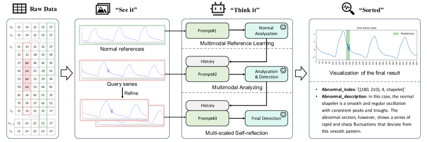
Figure 2. Our framework converts time series into images for visual interpretation (“See it”). Then, LMMs are employed to analyze the visualized time series through Multimodal Reference Learning, Multimodal Analyzing, and Multi-scaled Self-reflection, ensuring self-consistency and stability in the analysis (”Think it”). Finally, the detected anomalous intervals are processed into the output format required for TSAD, providing descriptions and possible reasons for each anomaly (”Sorted”).

3. Methodology

Previous TSAD methods often rely on manual feature extraction or require large amounts of high-quality training data, along with extensive parameter tuning tailored to specific tasks. This reliance can lead to suboptimal performance and inefficiency. To overcome these limitations, we leverage the perceptual and reasoning capabilities of pretrained LMMs. Our approach transforms time series data into visual representations, enabling few-shot, high-performance, and robust anomaly detection. In this section, we first introduce the necessary preliminaries, followed by a detailed presentation of the TAMA framework.

3.1. Preliminary

Time series anomaly detection and classification . Consider a time series data $\mathbf{x}=(x_{1},\dots,x_{T})\in R^{T}$, where $x_{t}$ represents the sampled value at timestamp $t$. In this paper, we focus on univariate time series, while multivariate data will be converted into multiple univariate series. The goal of time series anomaly detection is to identify anomalous points or intervals within the time series $\mathbf{x}$. Specifically, an anomaly detection model outputs a sequence of anomaly scores $\mathbf{s}=(s_{1},\dots,s_{T})$, where $s_{t}$ indicates the anomaly score corresponding to the data point $x_{t}$. A higher anomaly score suggests that the model perceives a greater likelihood of the point being anomalous, while a lower score indicates a higher probability of the point being normal. By setting a threshold, the set of anomalous points can be obtained from the score sequence $\mathbf{s}$. Anomaly classification is a multi-class classification task designed to categorize identified anomalous points into specific types of anomalies. These anomaly types can provide insights into the characteristics and possibly the underlying causes of the detected anomalies.

Preprocessing. We follow common practice by applying mean-variance normalization to preprocess the time series, resulting in normalized data $\overline{\mathbf{x}}=(\overline{x}_{1},\dots,\overline{x}_{T})$, where $\overline{x}_{t}=\frac{x_{t}-\mu(\mathbf{x})}{\sigma(\mathbf{x})},$ with $\mu(\cdot)$ and $\sigma(\cdot)$ denoting the mean and standard deviation functions, respectively. Then we utilize overlapped sliding windows to segment the normalized data into a collection of sequence segmentations $\mathcal{P}=\{\hat{\mathbf{x}}_{1},\dots,\hat{\mathbf{x}}_{l}\}$, where $\hat{\mathbf{x}}_{k}=(\overline{x}_{k\cdot L_{s}},\dots,\overline{x}_{k\cdot L_{s}+L_{w}-1})$. $L_{s}$ and $L_{w}$ are hyperparameters representing the step size and width of the sliding window, respectively. The overlap ratio is defined as $r_{o}=L_{s}/L_{w}$. In this work, we choose $r_{o}<1$ to allow the same segment of the sequence to be considered across multiple windows.

Image Conversion. To leverage the multimodal reasoning capabilities of the pretrained LMMs, we convert the time series data into graphs, serving as image modality inputs for the model. To accommodate the token limitations of the model, we impose a resolution constraint on the images. Further details can be found in Appendix A.3.

3.2. Time Series Anomaly Analyzer  (TAMA)

The proposed TAMA framework is illustrated in Figure 2. TAMA comprises three sections that involve the participation of the LMM: Multimodal Reference Learning, Multimodal Analyzing, and Multi-scaled Self-reflection. Within these sections, we utilize specific prompts to guide the LMM in executing designated operations. A post-processing module is employed to integrate the model’s outputs and obtain the final results. All prompts used in the experiments are detailed in Appendix A.1. Below, we provide a detailed explanation of TAMA’s workflow.

Multimodal Reference Learning. This section leverages the few-shot in-context learning (ICL) capabilities of pretrained LMMs to capture the patterns of normal sequences. The model is provided with a set of normal images $\mathcal{I}=\{\mathbf{I}_{i}\mid i\in\{1,\dots,n_{r}\}\}$, where $n_{r}$ denotes the number of reference images. These reference images are accompanied by prompts indicating that they represent normal sequences without anomalies. The model is then tasked with generating descriptive outputs for these normal images. These descriptions will be used in subsequent interactions with the model, helping it to better focus on normal patterns and improving its ability to detect anomalous sequences.

Multimodal Analyzing. This section utilizes the normal data patterns learned by the LMMs during reference learning to identify anomalies in new samples. Specifically, the LMMs is driven to accomplish two tasks: anomaly detection and classification.

For the $k^{\text{th}}$ sliding window, the anomaly interval detection task requires the model to output a set of anomaly intervals $\mathcal{A}_{k}=\{(t_{s},t_{e})^{i}\}_{i=1}^{m_{k}}$, where $(t_{s},t_{e})^{i}$ represents the $i$th anomaly interval, and $m_{k}$ is the number of detected anomaly intervals within the sliding window. We require $t_{s}\leq t_{e}$ ($t_{s}=t_{e}$ indicates a point anomaly). Note that the intervals output by the LMMs are the indices within the sliding window, which will be converted to global indices during post-processing.

Based on the results of anomaly detection, the model is then tasked with classifying each detected interval. Following (Lai et al., 2021), anomalies are categorized into four types: point, shapelet, seasonal, and trend. We inform the LMMs about the characteristics of each type through natural language descriptions (see Prompt A.3 in Appendix). The LMMs will output an anomaly set $\mathcal{Y}_{k}=\{y_{i}\}_{i=1}^{m_{k}}$, where $y_{i}$ corresponds to the anomaly classification result for the interval $(t_{s},t_{e})^{i}$. Moreover, we also require the LMMs to provide a confidence score and an explanation for each detected anomaly interval, denoted as $\mathcal{C}_{k}=\{c_{i}\}_{i=1}^{m_{k}}$ and $\mathcal{T}_{k}=\{\text{E}_{i}\}_{i=1}^{m_{k}}$, respectively. Thus, traversing all sliding windows, the total output from the model is given by

$$\mathcal{Z}_{\text{raw}}=\{(\mathcal{A}_{k},\mathcal{Y}_{k},\mathcal{C}_{k},\mathcal{T}_{k})\}_{k=1}^{N},$$

where $N$ is the total number of sliding windows.

Multi-scaled Self-reflection. This section motivates the LMMs to correct some of its own errors, thereby enhancing the robustness and accuracy of anomaly detection. We provide the LMMs with the outputs from the previous sections, along with zoomed-in images of the detected anomaly regions. The zooming in on the anomaly areas helps prevent the model from repeatedly generating the same results due to viewing identical images. To save tokens, this operation is conducted only within the windows where some anomaly intervals are detected.

Results Aggregation. In the post-processing stage, we need to consolidate the overlapped sliding windows and establish a threshold to determine the final detected anomaly points. First, we convert the indices of the anomaly intervals within the windows to a unified set of global indices. Next, we perform pointwise addition of all predicted confidence scores, i.e., if a point is detected in multiple intervals, its confidence score is the sum of the confidence scores of all these intervals. As a result, we obtain a confidence sequence $\tilde{\mathbf{c}}=(\tilde{c}_{1},\dots,\tilde{c}_{T})$ that enjoys the same length as the original sequence. Similarly, a pointwise anomaly classification sequence $\tilde{\mathbf{y}}=(\tilde{y}_{1},\dots,\tilde{y}_{T})$ is obtained, where the classification result for each point is determined by a voting mechanism from all the anomaly intervals that contain the point. Finally, by setting a threshold $c_{0}$, we obtain the final set of anomaly points $\mathcal{R}=\{i\ |\ 1\leq i\leq T,\tilde{c}_{i}\geq c_{0}\}$.

Table 1. Quantitative results across six datasets use metrics point-adjusted F1%, AUC-PR%, and AUC-ROC%. Best and second-best results are in bold and underlined, respectively. TAMA represents our framework, and TAMA* represents our framework without self-reflection. Each unit in the table contains two value: mean and maxima of all series.

Dataset	UCR						NASA-SMAP						NASA-MSL
Metric	F1%		AUC-PR%		AUC-ROC%		F1%		AUC-PR%		AUC-ROC%		F1%		AUC-PR%		AUC-ROC%
IF	24.7	77.3	37.7	44.6	24.4	25.3	54.2	94.2	58.9	77.1	65.0	87.7	47.6	88.6	53.6	80.4	68.7	88.7
LOF	42.8	100	35.6	50.0	92.8	99.9	62.2	100	43.4	61.4	60.1	99.9	36.4	66.8	44.5	66.0	58.6	99.8
TranAD	38.2	93.7	30.9	51.0	77.0	99.9	59.0	99.6	36.8	73.9	74.4	100	64.6	99.1	49.2	79.6	82.5	99.9
GDN	71.4	80.6	33.4	59.0	87.1	99.9	76.4	100	40.8	66.2	86.1	100	85.1	100	38.7	56.7	93.8	100
MAD_GAN	74.2	85.0	51.5	65.9	99.4	99.9	61.3	100	39.9	72.3	83.3	100	96.0	100	46.4	50.0	95.7	100
MSCRED	32.6	96.0	28.9	45.9	94.2	99.9	57.0	97.9	40.8	61.7	77.0	100	63.0	92.2	39.5	51.8	73.2	98.1
MTAD_GAT	14.8	36.6	34.2	38.9	84.6	94.4	78.3	100	40.2	58.0	77.0	100	90.6	100	49.2	67.8	81.2	100
OmniAnomaly	34.5	95.7	26.0	45.9	85.6	99.9	57.1	100	43.6	63.2	77.5	100	71.4	100	40.0	74.9	85.0	99.9
USAD	57.6	100	33.1	50.0	97.1	99.9	72.8	100	43.6	63.2	93.9	100	91.6	99.9	42.6	60.8	94.2	100
TimesNet	32.8	45.8	15.4	23.5	98.4	99.4	97.7	100	51.4	90.3	99.8	100	97.4	100	52.9	79.7	99.8	100
SIGLLM (GPT-4o)	23.1	44.6	7.40	15.5	93.5	96.5	69.0	97.8	29.1	49.2	95.5	99.8	70.7	97.9	72.4	100	90.0	100
TAMA	92.5	97.6	93.0	97.7	99.8	99.9	94.5	100	95.5	100	98.4	100	97.5	100	99.4	100	99.8	100
TAMA*	92.5	97.6	93.0	97.7	99.8	99.9	87.8	100	89.2	100	97.0	100	96.1	100	97.7	100	99.0	100
Dataset	SMD						ECG						Dodgers
Metric	F1%		AUC-PR%		AUC-ROC%		F1%		AUC-PR%		AUC-ROC%		F1%		AUC-PR%		AUC-ROC%
IF	83.9	100	73.8	97.0	99.5	100	80.8	99.0	73.4	92.2	97.2	100	48.4	48.4	52.2	52.2	89.4	89.4
LOF	27.8	75.2	39.9	64.6	52.9	59.3	21.8	39.8	41.4	60.7	56.3	84.2	45.3	45.3	40.8	40.8	63.0	63.0
TranAD	77.0	99.6	70.9	91.0	96.8	100	69.1	98.9	74.7	97.7	94.9	100	38.2	38.2	33.9	33.9	74.6	74.6
GDN	76.9	99.7	55.0	88.6	77.0	100	75.2	96.2	76.6	97.4	96.9	99.9	37.0	37.0	31.3	31.3	74.2	74.2
MAD_GAN	67.1	92.6	61.7	87.5	91.7	100	79.1	99.3	79.2	97.6	96.9	100	32.2	32.2	28.6	28.6	74.7	74.7
MSCRED	69.4	95.7	55.8	96.2	95.0	100	66.4	99.0	73.8	97.2	88.7	100	37.8	37.8	30.6	30.6	74.6	74.6
MTAD_GAT	69.7	95.3	59.5	90.4	90.6	99.7	67.5	100	73.5	98.8	82.5	100	39.1	39.1	36.0	36.0	74.9	74.9
OmniAnomaly	66.0	96.4	61.6	91.8	87.7	100	76.8	98.6	76.4	97.5	93.5	100	33.6	33.6	35.4	35.4	60.3	60.3
USAD	72.2	99.7	67.8	93.5	94.4	100	71.5	96.9	75.2	98.3	94.9	100	37.8	37.8	33.1	33.1	74.6	74.6
TimesNet	82.8	100	57.3	99.9	95.4	100	92.4	96.6	90.0	97.6	99.4	100	48.1	48.1	73.0	73.0	83.7	83.7
SIGLLM (GPT-4o)	42.9	59.8	30.4	53.1	68.8	77.8	19.2	50.4	71.0	87.6	94.2	96.9	48.1	48.1	60.7	60.7	83.2	83.2
TAMA	77.8	100	87.9	100	98.9	100	81.3	87.5	84.5	90.0	95.4	99.4	65.6	65.6	74.0	74.0	85.2	85.2
TAMA*	62.8	93.0	78.6	97.2	99.7	99.7	78.1	88.0	83.4	91.1	94.7	99.1	64.5	64.5	73.6	73.6	85.3	85.3

4. Experiments

In this section, we conduct extensive experiments to evaluate TAMA. The experiments include Anomaly Detection and Anomaly Classification, and Ablation Study.

Experimental Settings. We select GPT-4o (OpenAI et al., 2024) TAMA’s default model, and the specific version we used is ”gpt-4o-2024-05-13”. To ensure the stability of TAMA and the reproducibility of the results, we set the temperature to 0.1 and set the top_p to 0.3. Besides, we use the JSON mode of GPT-4o to facilitate subsequent result analysis. All the prompts can be found in Appendix A.1. The detailed settings of image conversion has also been provided and discussed in Appendix A.3.

Datasets. As shown in Table 2, we use a diverse set of real-world datasets across multiple domains for both anomaly detection and anomaly classification tasks. These domains include Web service: SMD (Su et al., 2019), industry: UCR (Wu and Keogh, 2021), NormA (Boniol et al., 2021), NASA-SMAP (Hundman et al., 2018), and NASA-MSL (Hundman et al., 2018), health care: ECG (Paparrizos et al., 2022), and transportation: Dodgers (Hutchins, 2006). All datasets are univariate except for SMD, which is originally multivariate. We convert SMD into a univariate dataset by splitting it channel-wise for our anomaly detection experiment. The full experimental results are available in Appendix A.4.

Due to the limited availability of datasets with anomaly classification labels, we created an anomaly classification dataset by combining four real-world datasets (UCR, NASA-SMAP, NASA-MSL, and NormA) with manually labeled anomaly types, along with a synthetic dataset generated using GutenTAG (Wenig et al., 2022). To ensure the accuracy of the anomaly type annotations, cross-validation on the labels of the four real-world datasets was conducted by experts in each field. The synthetic dataset contains 7200 samples, and the anomaly types in this dataset are point, trend, and frequency, as derived from the work of Lai et al. (Lai et al., 2021). A visualization of each typical anomaly type is included in Appendix 7.

4.1. Anomaly Detection

In this section, we evaluate the anomaly detetcion capability of TAMA.

Table 2. Details of all datasets. Datasets with classification labels include real-world datasets we labeled (marked with ⁺) and a synthetic dataset (marked with ^∗) we generated using GutenTAG (Wenig et al., 2022). ”-” denotes corresponding training data does not exist or missing classification labels.

Dataset	#Train	#Test (labeled)	Anomaly%
			Point	Shapelet	Seasonal	Trend	Total
UCR+	1,200-3,000	4,500-6,301	0.04	1.05	0	0	1.10
SMAP+	312-2,881	4,453-8,640	0	7.0	0.2	0.1	7.3
MSL+	439-4,308	1,096-6,100	1.3	6.2	0	3.0	10.5
NormA+	-	104,000-196,000	0	18.6	4.1	1.2	24.0
Synthetic∗	3,600	3,600	0.3	0	3.4	1.4	5.1
SMD	23,687-28,743	23,687-28,743	-	-	-	-	4.2
Dodgers	-	50,400	-	-	-	-	11.1
ECG	227,900-267,228	227,900-267,228	-	-	-	-	7.9

Baselines. The baseline models used in our experiments include both machine learning algorithms  (IF (Liu et al., 2008), LOF (Huang et al., 2013)) and deep learning  (TranAD (Tuli et al., 2022), GDN (Deng and Hooi, 2021), MAD_GAN (Li et al., 2019), MSCRED (Zhang et al., 2018), MTAD_GAT (Zhao et al., 2020), OminiAnomaly (Su et al., 2019), USAD (Audibert et al., 2020) and TimesNet (Wu et al., 2023)). Besides, the SIGLLM (Alnegheimish et al., 2024) is a baseline model based on the LLM. We reproduce it with GPT-4o. All baseline models has been run with the default configurations. For those datasets without default configurations, we managed to optimize the performance by searching the best parameters.

Metrics. Following the mainstream of TSAD, we evaluated TAMA and other baselines by the point-adjusted F1 (Xu et al., 2018). Point adjustment (PA) is a widely used adjustment method in TSAD tasks (Kim et al., 2021; Blázquez-García et al., 2021), but it can significantly overestimate the models’ performances (especially F1), making it a subject of much debate. A detailed explanation and further discussion of are available in Appendix A.2.

To fully assess how the models’ performance at different levels of sensitivity and specificity, we also adopted two threshold-agnostic metrics, namely AUC-PR and AUC-ROC. We would like to highlight AUC-PR as it is more robust to scenarios with highly imbalanced classes (like TSAD) comparing to AUC-ROC (Sofaer et al., 2019).

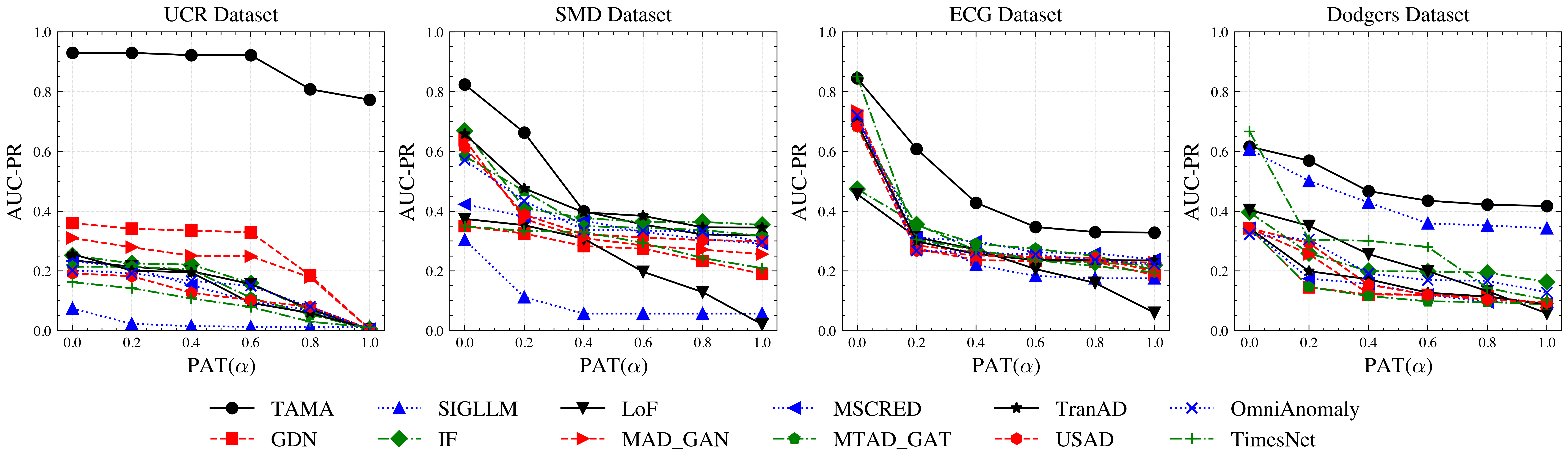
Figure 3. The AUC-PR of all models at various point-adjustment threshold $\alpha$ (PAT, defined in Appendix A.2).

Main Results. The experiment results are shown in Table 1. Each metric in the table contains two value: mean and maxima. The mean refers to the average of all sub-series, while the maxima represents the best result among all sub-series. For the maxima value, our method (TAMA) generates comparable results as other baseline models, even better in some datasets. TAMA outperforms almost all baseline models across every dataset in terms of mean metrics, especially on industry and transportation datasets. The exceptional performance of the mean suggests that our approach exhibits superior stability across a broader range of data. In contrast, most baseline models are sensitive to their hyper-parameters, leading to limited generalization.

Self-reflection. In order to improve the stability, we add the self-reflection to TAMA. The results are presented in Table 1. TAMA* represents the method without self-reflection. We can find that in most datasets, the maxima of TAMA* is very close to that of TAMA. However, there are obvious drops of mean in most datasets, especially in NASA-SMAP. These drops demonstrate the efficacy of self-reflection in stability.

The impact of point-adjustment. Under the point-adjustment, if a single point is predicted correctly in an interval, the entire interval is considered to be right, which greatly overestimates the model’s performance. To address this, we re-evaluate all models using point-adjustment with a threshold $\alpha$ (PAT, defined in Appendix A.2).

The results are shown in Figure 3 (full results in Appendix A.5.). We only present results of four datasets due to the limitation of the space, the full results are available in Appendix A.5. The UCR, SMD, ECG, and Dodgers datasets originate from the domains of industry, web services, healthcare, and transportation, respectively.

Based on the experimental results, we can find that the performance of all models declines as the PAT increases, indicating that full point-adjustment ($\alpha$=0) has overestimated the model performance. However, compared to other baseline methods, TAMA demonstrates excellent performance across all PATs, showing that TAMA can identify the anomaly more accurately.

Overall, the results of anomaly detection in Table 1 reveals that the LMM is an excellent and stable anomaly detector. The ability of multimodal reasoning can be utilized in analyzing the image of time series data and achieve an impressive standard.

4.2. Anomaly Classification

In practical applications, it is preferable not only to detect anomaly intervals but also to provide a brief classification indicating their causes. To fully demonstrate the strong reasoning capabilities of the proposed framework and enhance the interpretability of detection results, we conduct classification on the anomaly data.

Table 3. Classification results are detailed for each anomaly type, with ‘total’ representing the overall performance.

Type	Point	Shapelet	Seasonal	Trend	Total
Accuracy%	81.0	99.2	29.0	74.5	78.5
Support	100	246	100	94	567

The overall results presented in Table 3 indicate that TAMA, guided by the provided prompts (outlined in Appendix A.1), demonstrates a reliable understanding of each type of anomaly and can accurately classify most anomalies, with the exception of seasonal anomalies. TAMA performs exceptionally well in classifying shapelet anomalies, suggesting that it effectively captures the shape of the input sequences. However, it is evident that the framework struggles with seasonal anomalies. We interpret this difficulty as stemming from a lack of relevant materials in the LMM’s pre-training stage, which results in a weak understanding of concepts such as ”seasonality” or ”frequency”. More discussion on TAMA’s behavior to each anomaly type is included in Appendix A.6.

Table 4. Comparison of different pre-trained LMMs using the average AUC-PR% without PA as the metric. We compare results with (+TAMA) and without our framework (Naive).

LMM	Naive	+TAMA
GPT-4o	41.8	80.2 (+38.4)
GPT-4o-mini	11.8	51.1 (+39.3)
Gemini-1.5-pro	25.4	87.8 (+62.4)
Gemini-1.5-flash	17.9	36.4 (+18.5)
qwen-vl-max-0809	61.7	80.5 (+18.8)

4.3. Ablation Study

There are many hyperparameters affecting the performance of our framework. In this section, some ablation experiments are conducted to evaluate the impact of each hyperparameter, including LMM Selection, Reference Number and Window Size.

LMM Selection. In this section, we valid that the design of TAMA enhances the capability of LMMs in anomaly detection task. We conduct experiments on the UCR dataset with various LMMs, including GPT-4o, GPT-4o-mini, Gemini-1.5-pro, Gemini-1.5-flash, and Qwen-vl-max. For each LMM, we conduct experiments both with  (+TAMA) and without  (Naive) TAMA framework. Due to budget constraints, we only conduct this experiment on the UCR dataset. However, we believe the experimental results can, to some extent, reflect real-world scenarios.

The experimental results are presented in the Table 4. To better evaluate the efficacy of our framework (TAMA), we use the original AUC-PR without point-adjustment as the metric in this experiment. The findings reveal that all LMMs exhibit a substantial enhancement in performance on the UCR dataset following their integration into TAMA. This not only validates that TAMA improves the LMMs’ abilities in anomaly detection but also confirms the generalizability of TAMA’s framework.

Reference Number. As mentioned earlier in Section 3.2, we provide some normal images $\mathbf{I}=\{I_{i}|i\in[1,N]\}$ as references to help the LMM learn the distribution of normal data. In this ablation experiment, we investigate the impact of the number of reference images $N$. The ablation experiment is conducted on UCR and NASA-SMAP datasets. The ablation experiment is conducted on the UCR and NASA-SMAP datasets. To more clearly highlight the differences in performance, we used metrics without PA. Moreover, to avoid interference from other modules and more realistically demonstrate the role of Multimodal Reference Learning, self-reflection is not added in this ablation experiment.

As shown in the Figure 4, when the Reference Number is set to 0, which indicates that no reference is provided in the framework, the performance has a significant drop. As the number of Reference Number increases, although there are some fluctuations, it remains relatively stable, and the performance is considerably improved to the case without references.

Our results show that using Reference Learning is highly necessary, as it can significantly improve the method’s performance and stability. At the same time, from the experimental results, we also find that the quantity of references, from 1 to 4, does not seem to have a clear relationship with the final results. However, in case of the random sampling of normal data, setting the Reference Number to 3 can enhance overall robustness.

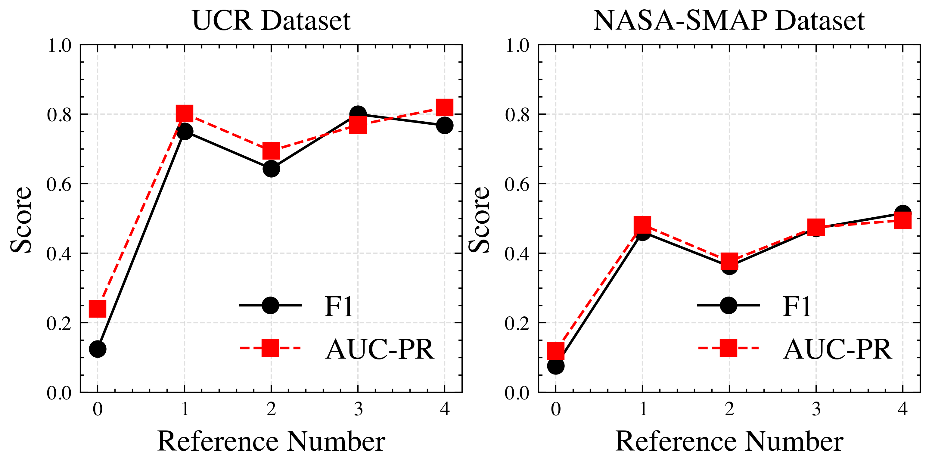
Figure 4. Results (without PA) of reference number ablation experiments.

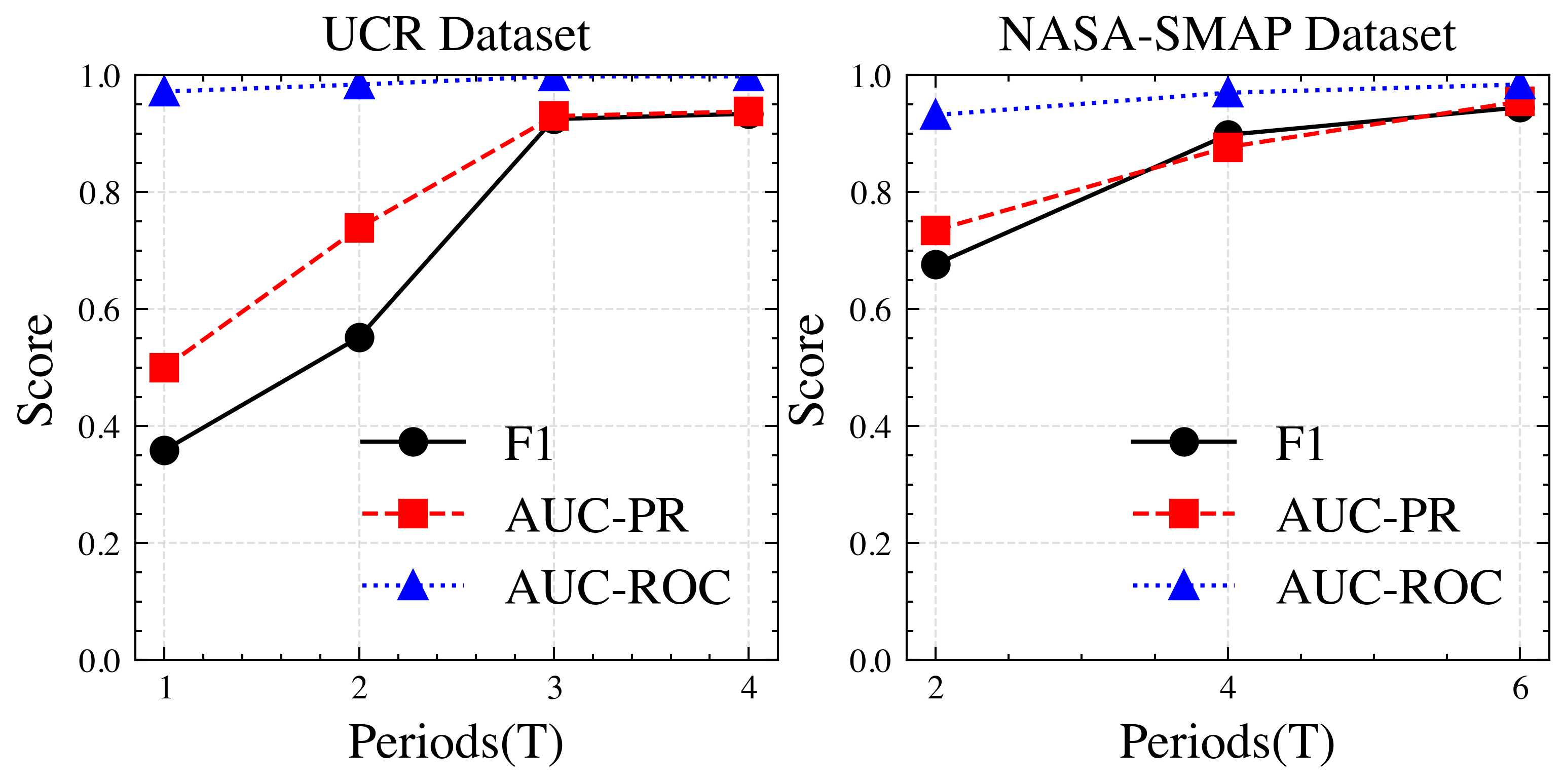
Figure 5. Results of window size ablation experiments. For the period of two datasets, $T_{UCR}\approx 200$, $T_{NASA-SMAP}\approx 100$

Window Size. In TAMA, as it shown before (in Section 3.1), we use sliding window in the data pre-processing stage. To accommodate different time series data with varying periods, we report the window size in multiples of the data period.

The results presented in Figure 5 reveal that the performance of our method is positively correlated with the window size. This is because the LMMs struggles to identify periodic patterns when given only single-period images, resulting in incorrectly classifying periodic features and truncated features as anomalies. Therefore, we ultimately set the window size to approximately $3T$ for the experiments detailed in Section 4.1.

5. Discussion

In this section. we reflect on the design of TAMA and seek to answer the following research questions:

RQ1: Is the image modality better than text modality for LMMs in the time series anomaly detection task? (Section 5.1)

RQ2: How does the additional information on images affect the LMM’s analysis? (Section 5.2)

RQ3: Dose the LMM truly learn the reference data during the multimodal Rederence Learning. (Section 5.3)

5.1. Modality

To investigate whether the success of our framework comes from the more advanced model (GPT-4o) we choose or the image-modality. we conduct an experiment in NASA-MSL and NASA-SMAP datasets, which both are real-world datasets and have more complex patterns than the UCR dataset.

The results are shown in Table 5. We choose different modalities for testing while trying to keep the prompts and procedures as the same. To maintain fairness, we do not add the self-reflection in TAMA. Meanwhile, we also include the results of SIGLLM (Alnegheimish et al., 2024), which uses Mistral-7B, as a reference. Compared to methods using text-modality, TAMA  (Image), which use image-modality, has made significant improvement, with a 37.9% increase on NASA-MSL and a 36.9% increase on NASA-SMAP. This result indicates that for anomaly detection tasks, allowing the model to ”see” time series data  (using image modality) is more beneficial. It also demonstrates that multimodal reasoning has tremendous promise in time series anomaly detection tasks.

Table 5. The performance comparison of image and text modalities, using the average PA F1% as the metric. TAMA (Image) and TAMA (Text) are based on TAMA but using image-modality and text-modality respectively.

Modality	NASA-MSL	NASA-SMAP
TAMA (Image)	97.5	94.5
TAMA (Text)	70.7	69.0
SIGLLM (Text) (Alnegheimish et al., 2024)	42.9	43.1

5.2. Additional Information in Images

The transformation of raw data into visual formats, such as images, adds crucial information, including plot orientation and auxiliary lines. This study investigates how these elements influence TAMA’s performance in identifying abnormal intervals based on plot scales. We conducted two experiments: the first involved rotating images by 90 degrees before inputting them into TAMA, while the second examined the impact of auxiliary lines, which are perpendicular to the x-axis and align with the scale to aid in locating data points.

Both experiments are performed on the UCR and NASA-SMAP datasets. Results are presented in Table 6, where TAMA represents the original model, TAMA-R indicates performance with rotated images, and TAMA-A reflects performance without auxiliary lines. We evaluated using the AUC-PR without point adjustment. The findings demonstrate a notable decline in TAMA-R’s performance with rotated images, suggesting that the LMMs are sensitive to image orientation. Despite the rotation of axis is disturbed in prompts, the LMM struggles to interpret rotated images accurately, leading to reduced anomaly detection. In contrast, TAMA-A experiences only a slight performance decrease across both datasets, indicating that LMMs can better identify abnormal intervals when auxiliary lines are present.

These experiments reveal that LMMs perceive time series images similarly to humans— uxiliary lines enhance anomaly localization accuracy, while image rotation negatively affects performance. This sensitivity may result from the tokenizer’s responsiveness to orientation or insufficient training data and guidance.

Table 6. The average AUC-PR% performance of TAMA with different additional information in images.

Datasets	TAMA	TAMA-R	TAMA-A
UCR	83.0	32.9 (-50.1)	75.6 (-7.60)
NASA-SMAP	72.9	28.6 (-44.3)	66.4 (-6.50)

Table 7. The performance comparison in different reference images, using the AUC-PR% without PA as the metric.

Dataset	normal	abnormal
UCR	83.0	46.8 (-36.2)
NASA-SMAP	72.9	48.5 (-24.4)

5.3. Multimodal Reference Learning

We provide a set of images for LMMs, helping LMMs to better focus on normal pattern and improving the ability to detect anomalous intervals (Section 3.2). To study whether the LMM truly learns from the reference images, we conduct this experiment on the UCR and NASA-SMAP datasets, replacing the normal data with abnormal data, and Multi-scaled Self-reflection is not enabled in this experiment. The results are presented in Table 7. In the table, normal refers to using the normal data as the reference data, while abnormal indicates using abnormal data as reference data. The experimental results under different reference data conditions are evaluated by the AUC-PR without point-adjustment. We can find that normal performs better than abnormal on both UCR and NASA-SMAP datasets, showing that the content for reference learning can notably impact the model’s performance, which suggests the LMM can truly learn normal representation from the reference data.

6. Conclusion

In this paper, we introduced TAMA, a novel framework that leverages large multimodal models for effective time series anomaly analysis. Comprehensive evaluation across multiple metrics demonstrates that TAMA not only surpasses state-of-the-art methods but also provides valuable semantic classifications and insights into detected anomalies. By converting time series data into visual representations, we have, for the first time, applied large multimodal models to this domain, enabling stronger generalization and more robust interpretative analysis. In summary, TAMA represents a significant advancement in anomaly detection methodologies, with practical implications for real-world applications and new opportunities for future research in multidimensional anomaly detection.

However, some limitations should be noted. Firstly, the proposed approach primarily relies on the pre-trained LMMs without fine-tuning. Additionally, in this work, we only consider univariate time-series anomaly detection tasks, whereas in real-world scenarios, it’s necessary to incorporate multiple time series for comprehensive judgment. In future works, we plan to explore deploying large models locally and fine-tuning them to achieve better performance and enhanced data security. Furthermore, we are considering the incorporation of multidimensional time series anomaly detection in our subsequent research efforts.

Appendix A Appendices

A.1. Prompts

The design of prompts is based on the documentation of OpenAI. Writing the steps out explicitly can make it easier for the model to follow them. In our task, we separate the whole task into three specific tasks: Multimodal Reference Learning (see Prompt A.3), multimodal Analyzing (see Prompt A.3) and Multi-scaled Self-reflection (see Prompt A.3). Besides, we also provide some background information, such as siliding windows and additional information of images. With the JSON mode output of GPT-4o, it is very convenient for us to process the output results, requiring a detailed description of the output format in prompts. Based on our practical experience, we find that clear descriptions and a structured format significantly are very helpful for LMM to understand.

A.2. Point Adjustment Metrics

Given a set of real anomalous intervals $\mathcal{A}_{\text{T}}=\{(t_{s},t_{e})^{i}_{\text{T}}\}_{i=1}^{m_{T}}$ and a set of predicted anomalous intervals $\mathcal{A}_{\text{P}}=\{(t_{s},t_{e})^{i}_{\text{P}}\}_{i=1}^{m_{P}}$, the point-adjusted prediction $\mathcal{A}_{\text{PA}}$ is defined as:

(1) $$\mathcal{A}_{\text{PA}}=\mathcal{A}_{\text{P}}\cup\{t|t\in(t_{s},t_{e})^{i}_{\text{T}},|(t_{s},t_{e})^{i}_{\text{T}}\cap(t_{s},t_{e})^{j}_{\text{P}}|>0\},$$

where the $\mathcal{A}_{\text{PA}}$ is a set of points, $m_{T}$ and $m_{P}$ refer to the total number of real anomalous intervals and the total number of the LLM’s prediction, respectively. After point-adjustment, the point-adjusted Recall, Precision and F1 can be calculated as:

(2) $$R =\emph{Recall}~{}(\mathcal{A}_{\text{T}},\mathcal{A}_{\text{PA}}),$$

(3) $$P =\emph{Precision}~{}(\mathcal{A}_{\text{T}},\mathcal{A}_{\text{PA}}),$$

(4) F1 $$={2~{}(R+P)}/{~{}(R\cdot P)},$$

The point-adjustment with threshold $\alpha$ is defined as:

(5) $$\mathcal{A}_{\text{PA}}(\alpha) =\mathcal{A}_{\text{P}}\cup\{t|t\in(t_{s},t_{e})^{i}_{\text{T}},$$

$$\quad|(t_{s},t_{e})^{i}_{\text{T}}\cap(t_{s},t_{e})^{j}_{\text{P}}|>\alpha\cdot L((t_{s},t_{e})^{i}_{\text{T}})\}.$$

where $\alpha$ refers to the point-adjustment threshold (PAT) from 0 to 1, where 0 represents full point-adjustment $\mathcal{A}_{\text{PA}}$ and 1 represents original prediction $\mathcal{A}_{\text{P}}$, and the $L((t_{s},t_{e})^{i}_{\text{T}})$ refers to the length of $(t_{s},t_{e})^{i}_{\text{T}}$.

A.3. Some Suggestions about TAMA

In this paper, we propose a framework named TAMA to utilize the LMM to analyze time series images. However, we have tried multiple versions and gained valuable practical experience during the development process. Based on our practical experience, we provide some suggestions.

• To better parse the output results, choosing the LMM which supports JSON mode output or structured output can be very convenient. If the LMM does not support these output format, we can use GPT-4o, which supports structured output, to format the output text.

• Assume the period of series data is $T$, it is recommended to set the sliding window length to at least $3T$.

• The LMM marks the interval with anomaly based on the scale of the plot. Therefore, the scale of axis should be clear enough. However, the rotation of scale does not matter.

• Grid-like auxiliary lines can be added to enhance the accuracy of the anomaly intervals output by the LMM.

• According to the documentation of OpenAI, in order to use high revolution mode, the figure size should not larger than 2000x768 pixels. All images in TAMA will be limited to this size.

[hb]

[ht]

[t]

A.4. Full Results of Anomaly Detection across All Datasets

In this section, we present the full results of all datasets in Table 8. Due to the limitation of the space, we only present some of them in the main body. Meanwhile, we also present the variance in this table. Most of datasets contain more than one sub-sequence, to fully present and compare the performance, we evaluate all metrics in all sub-sequence and calculate three values: mean, variance and maxima. In this table, mean and variance are formated as ”mean $\pm$ variance”.

Table 8. Quantitative results across six datasets use metrics point-adjusted F1, AUC-PR, and AUC-ROC. Best and second-best results are in bold and underlined, respectively. TAMA represents our framework, and TAMA* represents our framework without self-reflection. Each unit in the table contains two value: mean and maxima of all series. The number following the mean represents the standard deviation (std) computed over all sequences.

Dataset	UCR						NASA-SMAP						NASA-MSL
Metric	F1%		AUC-PR%		AUC-ROC%		F1%		AUC-PR%		AUC-ROC%		F1%		AUC-PR%		AUC-ROC%
IF	24.7 $\pm$ 31.6	77.3	37.7 $\pm$ 15.0	44.6	24.4 $\pm$ 9.80	25.3	54.2 $\pm$ 36.4	94.2	58.9 $\pm$ 18.9	77.1	65.0 $\pm$ 6.10	87.7	47.6 $\pm$ 8.00	88.6	53.6 $\pm$ 4.80	80.4	68.7 $\pm$ 9.40	88.7
LOF	42.8 $\pm$ 1.10	100	35.6 $\pm$ 1.00	50.0	92.8 $\pm$ 19.2	99.9	62.2 $\pm$ 12.1	100	43.4 $\pm$ 12.9	61.4	60.1 $\pm$ 19.9	99.9	36.4 $\pm$ 25.3	66.8	44.5 $\pm$ 9.90	66.0	58.6 $\pm$ 0.50	99.8
TranAD	38.2 $\pm$ 40.7	93.7	30.9 $\pm$ 6.40	51.0	77.0 $\pm$ 26.8	99.9	59.0 $\pm$ 39.9	99.6	36.8 $\pm$ 19.1	73.9	74.4 $\pm$ 27.7	100	64.6 $\pm$ 38.6	99.1	49.2 $\pm$ 20.4	79.6	82.5 $\pm$ 18.3	99.9
GDN	71.4 $\pm$ 43.1	80.6	33.4 $\pm$ 0.40	59.0	87.1 $\pm$ 24.1	99.9	76.4 $\pm$ 38.5	100	40.8 $\pm$ 19.1	66.2	86.1 $\pm$ 27.7	100	85.1 $\pm$ 26.1	100	38.7 $\pm$ 9.90	56.7	93.8 $\pm$ 0.50	100
MAD_GAN	74.2 $\pm$ 40.4	85.0	51.5 $\pm$ 0.80	65.9	99.4 $\pm$ 1.30	99.9	61.3 $\pm$ 41.3	100	39.9 $\pm$ 19.1	72.3	83.3 $\pm$ 15.1	100	96.0 $\pm$ 5.60	100	46.4 $\pm$ 17.5	50.0	95.7 $\pm$ 7.10	100
MSCRED	32.6 $\pm$ 37.9	96.0	28.9 $\pm$ 2.70	45.9	94.2 $\pm$ 3.60	99.9	57.0 $\pm$ 44.2	97.9	40.8 $\pm$ 19.1	61.7	77.0 $\pm$ 28.2	100	63.0 $\pm$ 37.0	92.2	39.5 $\pm$ 16.3	51.8	73.2 $\pm$ 16.1	98.1
MTAD_GAT	14.8 $\pm$ 13.2	36.6	34.2 $\pm$ 4.80	38.9	84.6 $\pm$ 7.60	94.4	78.3 $\pm$ 37.7	100	40.2 $\pm$ 22.9	58.0	77.0 $\pm$ 12.3	100	90.6 $\pm$ 27.7	100	49.2 $\pm$ 9.70	67.8	81.2 $\pm$ 21.9	100
OmniAnomaly	34.5 $\pm$ 32.7	95.7	26.0 $\pm$ 0.30	45.9	85.6 $\pm$ 10.3	99.9	57.1 $\pm$ 39.9	100	43.6 $\pm$ 20.5	63.2	77.5 $\pm$ 24.8	100	71.4 $\pm$ 36.5	100	40.0 $\pm$ 17.2	74.9	85.0 $\pm$ 18.7	99.9
USAD	57.6 $\pm$ 35.6	100	33.1 $\pm$0.40	50.0	97.1 $\pm$ 4.20	99.9	72.8 $\pm$ 35.8	100	43.6 $\pm$ 22.5	63.2	93.9 $\pm$ 9.10	100	91.6 $\pm$ 26.2	99.9	42.6 $\pm$ 9.90	60.8	94.2 $\pm$ 0.70	100
TimesNet	32.8 $\pm$ 8.30	45.8	15.4 $\pm$ 5.20	23.5	98.4 $\pm$ 1.10	99.4	97.7 $\pm$ 3.50	100	51.4 $\pm$ 2.80	90.3	99.8 $\pm$ 0.09	100	97.4 $\pm$ 4.70	100	52.9 $\pm$ 8.10	79.7	99.8 $\pm$ 0.50	100
SIGLLM (GPT-4o)	23.1 $\pm$ 19.7	44.6	7.40 $\pm$ 6.70	15.5	93.5 $\pm$ 16.9	96.5	69.0 $\pm$ 34.4	97.8	29.1 $\pm$ 28.4	49.2	95.5 $\pm$ 3.60	99.8	70.7 $\pm$ 44.8	97.9	72.4 $\pm$ 28.6	100	90.0 $\pm$ 15.3	100
TAMA	92.5 $\pm$ 17.9	97.6	93.0 $\pm$ 12.1	97.7	99.8 $\pm$ 0.10	99.9	94.5 $\pm$ 7.20	100	95.5 $\pm$ 9.30	100	98.4 $\pm$ 4.60	100	97.5 $\pm$ 2.10	100	99.4 $\pm$ 17.8	100	99.8 $\pm$ 0.20	100
TAMA*	92.5 $\pm$ 17.9	97.6	93.0 $\pm$ 12.1	97.7	99.8 $\pm$ 0.10	99.9	87.8 $\pm$ 31.3	100	89.2 $\pm$ 16.6	100	97.0 $\pm$ 4.10	100	96.1$\pm$ 4.30	100	97.7 $\pm$ 18.2	100	99.0 $\pm$ 0.20	100
Dataset	SMD						ECG						Dodgers
Metric	F1%		AUC-PR%		AUC-ROC%		F1%		AUC-PR%		AUC-ROC%		F1%		AUC-PR%		AUC-ROC%
IF	83.9 $\pm$ 13.2	100	73.8 $\pm$ 17.3	97.0	99.5 $\pm$ 0.50	100	80.8 $\pm$ 20.5	99.0	73.4 $\pm$ 18.8	92.2	97.2 $\pm$ 4.70	100	48.4 $\pm$ 0.00	48.4	52.2 $\pm$ 0.00	52.2	89.4 $\pm$ 0.00	89.4
LOF	27.8 $\pm$ 6.60	75.2	39.9 $\pm$ 1.90	64.6	52.9 $\pm$ 2.60	59.3	21.8 $\pm$ 12.0	39.8	41.4 $\pm$ 4.40	60.7	56.3 $\pm$ 10.8	84.2	45.3 $\pm$ 0.00	45.3	40.8 $\pm$ 0.00	40.8	63.0 $\pm$ 0.00	63.0
TranAD	77.0 $\pm$ 33.0	99.6	70.9 $\pm$ 31.9	91.0	96.8 $\pm$ 13.3	100	69.1 $\pm$ 23.2	98.9	74.7 $\pm$ 22.9	97.7	94.9 $\pm$ 6.30	100	38.2 $\pm$ 0.00	38.2	33.9 $\pm$ 0.00	33.9	74.6 $\pm$ 0.00	74.6
GDN	76.9 $\pm$ 0.90	99.7	55.0 $\pm$ 35.5	88.6	77.0 $\pm$ 1.60	100	75.2 $\pm$ 17.6	96.2	76.6 $\pm$ 17.5	97.4	96.9 $\pm$ 3.70	99.9	37.0 $\pm$ 0.00	37.0	31.3 $\pm$ 0.00	31.3	74.2 $\pm$ 0.00	74.2
MAD_GAN	67.1 $\pm$ 1.30	92.6	61.7 $\pm$ 37.2	87.5	91.7 $\pm$ 1.60	100	79.1 $\pm$ 19.5	99.3	79.2 $\pm$ 19.4	97.6	96.9 $\pm$ 3.80	100	32.2 $\pm$ 0.00	32.2	28.6 $\pm$ 0.00	28.6	74.7 $\pm$ 0.00	74.7
MSCRED	69.4 $\pm$ 30.2	95.7	55.8 $\pm$ 36.7	96.2	95.0 $\pm$ 14.5	100	66.4 $\pm$ 26.3	99.0	73.8 $\pm$ 22.6	97.2	88.7 $\pm$ 13.5	100	37.8 $\pm$ 0.00	37.8	30.6 $\pm$ 0.00	30.6	74.6 $\pm$ 0.00	74.6
MTAD_GAT	69.7 $\pm$ 18.5	95.3	59.5 $\pm$ 33.8	90.4	90.6 $\pm$ 6.00	99.7	67.5 $\pm$ 29.2	100	73.5 $\pm$ 23.8	98.8	82.5 $\pm$ 17.1	100	39.1 $\pm$ 0.00	39.1	36.0 $\pm$ 0.00	36.0	74.9 $\pm$ 0.00	74.9
OmniAnomaly	66.0 $\pm$ 6.80	96.4	61.6 $\pm$ 34.2	91.8	87.7 $\pm$ 2.60	100	76.8 $\pm$ 21.3	98.6	76.4 $\pm$ 24.0	97.5	93.5 $\pm$ 8.80	100	33.6 $\pm$ 0.00	33.6	35.4 $\pm$ 0.00	35.4	60.3 $\pm$ 0.00	60.3
USAD	72.2 $\pm$ 0.30	99.7	67.8 $\pm$ 35.6	93.5	94.4 $\pm$ 1.60	100	71.5 $\pm$ 20.8	96.9	75.2 $\pm$ 18.9	98.3	94.9 $\pm$ 5.90	100	37.8 $\pm$ 0.00	37.8	33.1 $\pm$ 0.00	33.1	74.6 $\pm$ 0.00	74.6
TimesNet	82.8 $\pm$ 25.3	100	57.3 $\pm$ 21.2	99.9	95.4 $\pm$ 11.3	100	92.4 $\pm$ 3.70	96.6	90.0 $\pm$ 5.60	97.6	99.4 $\pm$ 0.40	100	48.1 $\pm$ 0.00	48.1	73.0 $\pm$ 0.00	73.0	83.7 $\pm$ 0.00	83.7
SIGLLM (GPT-4o)	42.9 $\pm$ 27.9	59.8	30.4 $\pm$ 21.0	53.1	68.8 $\pm$ 12.8	77.8	19.2 $\pm$ 13.7	50.4	71.0 $\pm$ 25.3	87.6	94.2 $\pm$ 3.20	96.9	48.1 $\pm$ 0.00	48.1	60.7 $\pm$ 0.00	60.7	83.2 $\pm$ 0.00	83.2
TAMA	77.8 $\pm$ 17.1	100	87.9 $\pm$ 10.4	100	98.9 $\pm$ 1.40	100	81.3 $\pm$ 19.1	87.5	84.5 $\pm$ 15.4	90.0	95.4 $\pm$ 2.30	99.4	65.6 $\pm$ 0.00	65.6	74.0 $\pm$ 0.00	74.0	85.2 $\pm$ 0.00	85.2
TAMA*	62.8 $\pm$ 24.5	93.0	78.6 $\pm$ 14.1	97.2	99.7 $\pm$ 1.50	99.7	78.1 $\pm$ 19.8	88.0	83.4 $\pm$ 14.6	91.1	94.7 $\pm$ 2.50	99.1	64.5 $\pm$ 0.00	64.5	73.6 $\pm$ 0.00	73.6	85.3 $\pm$ 0.00	85.3
Dataset	NormA
Metric	F1%		AUC-PR%		AUC-ROC%
IF	56.8 $\pm$ 19.2	86.3	52.3 $\pm$ 21.9	81.2	57.9 $\pm$ 1.00	68.7
LOF	54.5 $\pm$ 17.8	77.9	68.8 $\pm$ 9.30	92.4	95.1 $\pm$ 2.90	97.9
TranAD	38.0 $\pm$ 15.8	76.0	49.7 $\pm$ 21.3	78.9	53.6 $\pm$ 2.00	83.6
GDN	38.5 $\pm$ 14.8	74.7	50.9 $\pm$ 20.2	78.3	54.2 $\pm$ 2.10	82.2
MAD_GAN	38.5 $\pm$ 14.3	74.7	51.1 $\pm$ 19.8	77.8	54.1 $\pm$ 2.90	81.9
MSCRED	38.4 $\pm$ 16.1	74.6	49.7 $\pm$ 20.9	77.7	53.8 $\pm$ 2.00	81.8
MTAD_GAT	49.7 $\pm$ 13.7	93.8	50.1 $\pm$ 21.3	95.6	66.6 $\pm$ 3.30	94.2
OminiAnomaly	43.2 $\pm$ 17.9	74.8	53.5 $\pm$ 20.3	79.1	49.8 $\pm$ 1.70	89.9
USAD	38.6 $\pm$ 15.9	75.6	53.3 $\pm$ 20.9	78.5	54.1 $\pm$ 1.70	82.9
SIGLLM (GPT-4o)	82.8 $\pm$ 30.0	94.6	93.8 $\pm$ 21.4	98.9	97.9 $\pm$ 2.50	99.1
TAMA	80.7 $\pm$ 4.70	89.2	95.0 $\pm$ 7.60	98.5	98.1 $\pm$ 0.70	99.2
TAMA*	83.9 $\pm$ 10.0	85.5	93.9 $\pm$ 10.8	98.7	97.4 $\pm$ 1.00	98.6

A.5. Full Results of the PAT Experiment

In Section 4.1, in order to study the impact of point-adjustment, we re-evaluate the results using the point-adjustment with a threshold $\alpha$ (See Appendix A.2). Due to the limitation of the space, we only present results of some datasets in the main body. The full results are presented in Figure 6. As the figure presented, our framework achieves outstanding AUC-PR across all datasets at various $\alpha$, showing that our framwork has better robustness and stability.

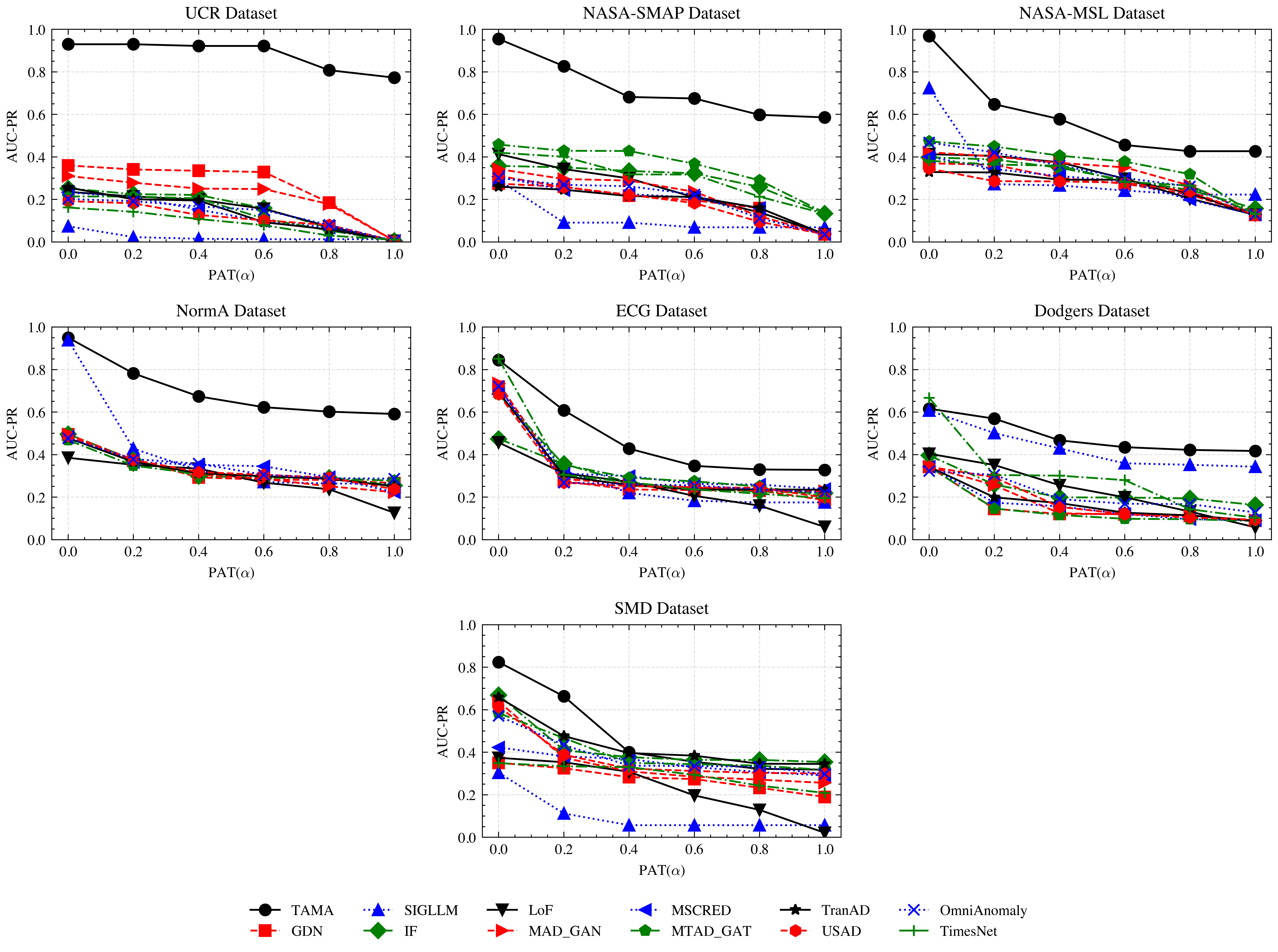
Figure 6. The full AUC-PR results of all models across all datasets at various point-adjustment threshold $\alpha$ (PAT, see Appendix A.2).

A.6. Performance Evaluation of Type-Specific Anomaly Detection Methods

Table 9. Quantitative results on each specific anomaly category across five datasets using F1-score% without point-adjustment. Best and second-best results are in bold and underlined, respectively. TAMA represents our framework (Some datasets include more than one series. To present the true performance of each method as much as possible, each unit in the table contains two values: maxima / mean. The maxima represents the best result among all sub-series, while the mean refers to the average of all sub-series.).

Dataset	NASA-MSL			NASA-SMAP			UCR
Category	Point	Shapelet	Trend	Shapelet	Seasonal	Trend	Point	Shapelet
TranAD	23.2 / 10.4	14.9 / 13.5	33.7 / 33.7	1.00 / 0.60	1.40 / 1.40	0.30 / 0.30	0.30 / 0.30	10.5 / 3.60
GDN	3.80 / 2.30	17.6 / 8.60	1.20 / 1.20	6.30 / 2.10	1.20 / 1.20	0.30 / 0.30	22.2 / 22.2	53.0 / 20.6
MAD_GAN	3.90 / 2.00	17.6 / 8.50	1.60 / 1.60	10.2 / 3.00	1.20 / 1.20	0.65 / 0.65	14.0 / 14.0	36.8 / 15.0
MSCRED	61.9 / 23.0	16.6 / 8.00	23.4 / 23.4	1.00 / 0.60	0.70 / 0.70	0.30 / 0.30	0.45 / 0.45	2.40 / 0.80
MTAD_GAT	69.8 / 46.3	16.6 / 8.00	73.9 / 73.9	52.0 / 24.0	2.10 / 2.10	0.95 / 0.95	0.80 / 0.80	2.70 / 1.45
OmniAnomaly	5.40 / 1.80	3.70 / 1.80	2.80 / 2.80	1.00 / 0.40	0.65 / 0.65	0.45 / 0.45	0.55 / 0.55	3.00 / 1.00
USAD	13.0 / 7.50	16.6 / 8.10	4.30 / 4.30	0.60 / 0.30	1.20 / 1.20	1.25 / 1.25	5.30 / 5.30	11.9 / 4.50
IF	35.0 / 24.2	30.0 / 22.9	31.6 / 31.6	30.2 / 17.1	1.10 / 1.10	1.45 / 1.45	0.55 / 0.55	2.70 / 1.85
LoF	22.9 / 10.1	33.4 / 22.4	33.3 / 33.3	14.0 / 7.80	0.60 / 0.60	4.60 / 4.60	0.45 / 0.45	2.05 / 1.35
TimesNet	23.2 / 10.9	12.5 / 8.30	22.4 / 10.8	20.4 / 8.95	1.35 / 1.35	25.6 / 25.6	0.40 / 0.40	1.80 / 1.20
SIGLLM	10.8 / 5.70	1.60 / 0.80	23.9 / 23.9	30.3 / 12.6	20.2 / 20.2	2.65 / 2.65	0.85 / 0.85	11.2 / 4.80
TAMA	70.2 / 31.9	26.2 / 11.4	22.4 / 13.5	77.4 / 47.9	0.10 / 0.10	84.5 / 84.5	20.0 / 20.0	92.3 / 81.0
Dataset	NormA			Synthetic
Category	Shapelet	Seasonal	Trend	Point	Seasonal	Trend
TranAD	4.00 / 2.30	3.30 / 2.20	3.90 / 2.50	0.55 / 0.35	8.90 / 1.90	13.5 / 7.90
GDN	4.10 / 2.30	3.30 / 2.20	3.90 / 2.50	0.50 / 0.35	13.6 / 2.10	12.4 / 6.50
MAD_GAN	4.10 / 2.30	3.30 / 2.20	3.90 / 2.50	0.55 / 0.35	8.50 / 1.60	13.9 / 8.00
MSCRED	4.10 / 2.30	3.30 / 2.20	3.90 / 2.50	0.55 / 0.35	8.50 / 1.60	10.5 / 5.20
MTAD_GAT	4.90 / 1.40	1.30 / 0.90	1.70 / 1.10	0.55 / 0.40	6.30 / 1.80	13.3 / 6.25
OmniAnomaly	12.6 / 5.70	11.5 / 7.50	11.4 / 7.30	30.3 / 19.8	9.30 / 1.70	11.2 / 7.80
USAD	4.10 / 2.40	3.30 / 2.20	3.90 / 2.50	0.55 / 0.35	8.90 / 1.70	12.6 / 7.30
IF	21.4 / 13.2	17.0 / 12.9	13.9 / 11.9	36.2 / 21.6	10.4 / 9.05	10.9 / 7.20
LoF	30.7 / 16.8	25.7 / 18.6	21.5 / 16.9	0.50 / 0.50	10.9 / 9.10	5.35 / 5.25
TimesNet	10.2 / 9.05	5.25 / 5.20	1.79 / 1.60	37.5 / 25.5	11.9 / 9.50	10.6 / 5.70
SIGLLM	6.50 / 3.10	3.70 / 2.50	0.90 / 0.60	0.60 / 0.35	10.9 / 7.95	14.0 / 6.50
TAMA	56.8 / 37.1	38.8 / 28.1	45.2 / 34.3	3.90 / 1.80	27.1 / 18.4	14.1 / 8.20

Table 9 presents the type-specific anomaly detection performances. To maintain readability, only the F1-score without point adjustment is reported. The results highlight TAMA’s outstanding performance in identifying pattern anomalies, including shapelet, seasonal, and trend types, while most baseline models struggle in this aspect without point adjustment. For instance, on the UCR-shapelet dataset, TAMA outperformed the second-best detector (GDN) by a substantial margin of 293% in terms of the mean F1-score. This superiority stems from TAMA’s inherent ability to detect anomalous intervals. However, this characteristic may lead to lower F1-scores in the detection of point anomalies. In the synthetic dataset we generated, labels for point anomalies were strictly defined. While TAMA’s interval detection always encompassed the ground-truth anomalies, it also produced a significant number of false positives.

A.7. Visualization of anomaly classification

In Section 4.2, we make a new dataset for anomaly classification by labeling some real-world datasets and generating sequence. We also provide some visualization of these anomalies to better understand the different types of anomalies. The visualization of anomaly classification is shown in Figure 7. The dataset contain four classification: Point, Shapelet, Seasonal and Trend, which are referenced from the work (Lai et al., 2021).

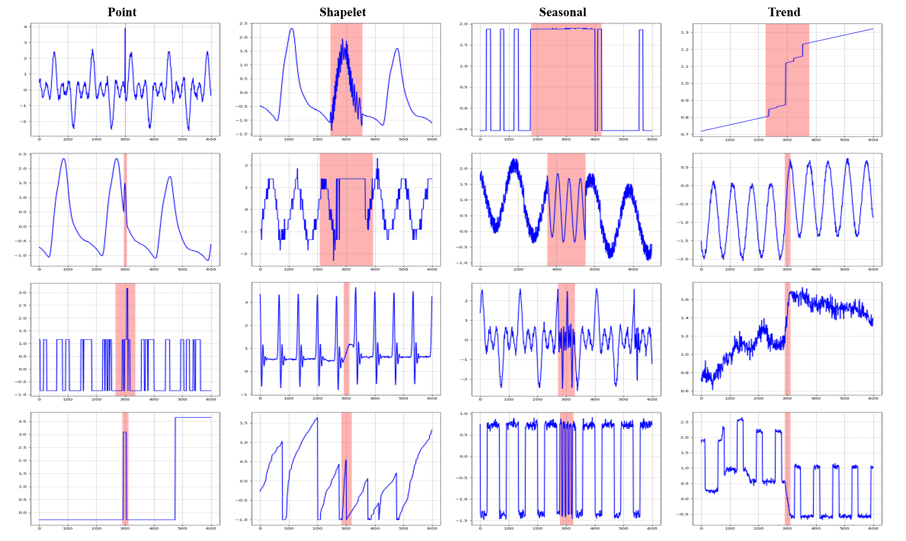
Figure 7. Visualization of anomalies. Each row displays sequences from different datasets that contain the same type of anomaly.

References

- (1)
- Alnegheimish et al. (2024) Sarah Alnegheimish, Linh Nguyen, Laure Berti-Equille, and Kalyan Veeramachaneni. 2024. Large language models can be zero-shot anomaly detectors for time series? https://arxiv.org/abs/2405.14755 _eprint: 2405.14755.
- Audibert et al. (2020) Julien Audibert, Pietro Michiardi, Frédéric Guyard, Sébastien Marti, and Maria A. Zuluaga. 2020. USAD: UnSupervised Anomaly Detection on Multivariate Time Series. In Proceedings of the 26th ACM SIGKDD International Conference on Knowledge Discovery & Data Mining (KDD ’20). Association for Computing Machinery, New York, NY, USA, 3395–3404. https://doi.org/10.1145/3394486.3403392 event-place: Virtual Event, CA, USA TLDR: A fast and stable method called UnSupervised Anomaly Detection for multivariate time series (USAD) based on adversely trained autoencoders capable of learning in an unsupervised way is proposed..
- Bandaragoda et al. (2014) Tharindu R. Bandaragoda, Kai Ming Ting, David Albrecht, Fei Tony Liu, and Jonathan R. Wells. 2014. Efficient Anomaly Detection by Isolation Using Nearest Neighbour Ensemble. In 2014 IEEE International Conference on Data Mining Workshop. 698–705. https://doi.org/10.1109/ICDMW.2014.70
- Blázquez-García et al. (2021) Ane Blázquez-García, Angel Conde, Usue Mori, and Jose A. Lozano. 2021. A Review on Outlier/Anomaly Detection in Time Series Data. ACM Comput. Surv. 54, 3 (April 2021). https://doi.org/10.1145/3444690 Place: New York, NY, USA Publisher: Association for Computing Machinery.
- Boniol et al. (2021) Paul Boniol, Michele Linardi, Federico Roncallo, Themis Palpanas, Mohammed Meftah, and Emmanuel Remy. 2021. Unsupervised and scalable subsequence anomaly detection in large data series. The VLDB Journal 30, 6 (Nov. 2021), 909–931. https://doi.org/10.1007/s00778-021-00655-8
- Bouasker et al. (2020) Taycir Bouasker, Mahjoub Langar, and Riadh Robbana. 2020. QoS monitor as a service. Software Quality Journal 28, 3 (Sept. 2020), 1279–1301. https://doi.org/10.1007/s11219-020-09514-1
- Brown et al. (2020) Tom B. Brown, Benjamin Mann, Nick Ryder, Melanie Subbiah, Jared Kaplan, Prafulla Dhariwal, Arvind Neelakantan, Pranav Shyam, Girish Sastry, Amanda Askell, Sandhini Agarwal, Ariel Herbert-Voss, Gretchen Krueger, Tom Henighan, Rewon Child, Aditya Ramesh, Daniel M. Ziegler, Jeffrey Wu, Clemens Winter, Christopher Hesse, Mark Chen, Eric Sigler, Mateusz Litwin, Scott Gray, Benjamin Chess, Jack Clark, Christopher Berner, Sam McCandlish, Alec Radford, Ilya Sutskever, and Dario Amodei. 2020. Language Models are Few-Shot Learners. https://arxiv.org/abs/2005.14165 _eprint: 2005.14165.
- Cao et al. (2021) Wenjie Cao, Cheng Zhang, Zhenzhen Xiong, Ting Wang, Junchao Chen, and Bengong Zhang. 2021. Image Classification of Time Series Based on Deep Convolutional Neural Network. In 2021 40th Chinese Control Conference (CCC). 8488–8491. https://doi.org/10.23919/CCC52363.2021.9550095
- Chalapathy and Chawla (2019) Raghavendra Chalapathy and Sanjay Chawla. 2019. Deep Learning for Anomaly Detection: A Survey. arXiv:1901.03407 [cs, stat] (Jan. 2019). http://arxiv.org/abs/1901.03407 arXiv: 1901.03407.
- Chang et al. (2024) Yupeng Chang, Xu Wang, Jindong Wang, Yuan Wu, Linyi Yang, Kaijie Zhu, Hao Chen, Xiaoyuan Yi, Cunxiang Wang, Yidong Wang, Wei Ye, Yue Zhang, Yi Chang, Philip S. Yu, Qiang Yang, and Xing Xie. 2024. A Survey on Evaluation of Large Language Models. ACM Trans. Intell. Syst. Technol. 15, 3 (March 2024). https://doi.org/10.1145/3641289 Place: New York, NY, USA Publisher: Association for Computing Machinery.
- Chen et al. (2024) Feiyi Chen, Zhen Qin, Mengchu Zhou, Yingying Zhang, Shuiguang Deng, Lunting Fan, Guansong Pang, and Qingsong Wen. 2024. LARA: A Light and Anti-overfitting Retraining Approach for Unsupervised Time Series Anomaly Detection. In Proceedings of the ACM Web Conference 2024 (WWW ’24). Association for Computing Machinery, New York, NY, USA, 4138–4149. https://doi.org/10.1145/3589334.3645472 event-place: Singapore, Singapore TLDR: In LARA, the retraining process is designed as a convex problem such that overfitting is prevented and the retraining process can converge fast, and it is mathematically and experimentally proved that when fine-tuning the latent vector and reconstructed data, the linear formations can achieve the least adjusting errors between the ground truths and the fine-tuned ones..
- Chen and Guestrin (2016) Tianqi Chen and Carlos Guestrin. 2016. XGBoost: A Scalable Tree Boosting System. In Proceedings of the 22nd ACM SIGKDD International Conference on Knowledge Discovery and Data Mining (KDD ’16). Association for Computing Machinery, New York, NY, USA, 785–794. https://doi.org/10.1145/2939672.2939785 event-place: San Francisco, California, USA.
- Choi et al. (2021) Kukjin Choi, Jihun Yi, Changhwa Park, and Sungroh Yoon. 2021. Deep Learning for Anomaly Detection in Time-Series Data: Review, Analysis, and Guidelines. IEEE Access 9 (2021), 120043–120065. https://doi.org/10.1109/ACCESS.2021.3107975
- Dai and Chen (2022) Enyan Dai and Jie Chen. 2022. Graph-Augmented Normalizing Flows for Anomaly Detection of Multiple Time Series. ArXiv abs/2202.07857 (2022). https://api.semanticscholar.org/CorpusID:246867225
- Deng and Hooi (2021) Ailin Deng and Bryan Hooi. 2021. Graph Neural Network-Based Anomaly Detection in Multivariate Time Series. In AAAI Conference on Artificial Intelligence. https://api.semanticscholar.org/CorpusID:231646473
- Elhafsi et al. (2023) Amine Elhafsi, Rohan Sinha, Christopher Agia, Edward Schmerling, Issa A. D. Nesnas, and Marco Pavone. 2023. Semantic anomaly detection with large language models. Autonomous Robots 47, 8 (Dec. 2023), 1035–1055. https://doi.org/10.1007/s10514-023-10132-6
- Fahim and Sillitti (2019) Muhammad Fahim and Alberto Sillitti. 2019. Anomaly Detection, Analysis and Prediction Techniques in IoT Environment: A Systematic Literature Review. IEEE Access 7 (2019), 81664–81681. https://doi.org/10.1109/ACCESS.2019.2921912 TLDR: This paper presents the results of a systematic literature review about anomaly detection techniques except for these dominant research areas, published from 2000 to 2018 in the application areas of intelligent inhabitant environments, transportation systems, health care systems, smart objects, and industrial systems..
- Feng et al. (2019) Cheng Feng, Venkata Reddy Palleti, Aditya P. Mathur, and Deeph Chana. 2019. A Systematic Framework to Generate Invariants for Anomaly Detection in Industrial Control Systems. Proceedings 2019 Network and Distributed System Security Symposium (2019). https://api.semanticscholar.org/CorpusID:142503744
- Gruver et al. (2024) Nate Gruver, Marc Finzi, Shikai Qiu, and Andrew Gordon Wilson. 2024. Large Language Models Are Zero-Shot Time Series Forecasters. https://doi.org/10.48550/arXiv.2310.07820 arXiv:2310.07820 [cs] TLDR: This work proposes procedures for effectively tokenizing time series data and converting discrete distributions over tokens into highly flexible densities over continuous values and shows how LLMs can naturally handle missing data without imputation through non-numerical text, accommodate textual side information, and answer questions to help explain predictions..
- Huang et al. (2013) Tian Huang, Yan Zhu, Qiannan Zhang, Yongxin Zhu, Dongyang Wang, Meikang Qiu, and Lei Liu. 2013. An LOF-Based Adaptive Anomaly Detection Scheme for Cloud Computing. In 2013 IEEE 37th Annual Computer Software and Applications Conference Workshops. 206–211. https://doi.org/10.1109/COMPSACW.2013.28 TLDR: This work presents an adaptive anomaly detection scheme for cloud computing based on LOF, which learns behaviors of applications both in training and detecting phase and enables the ability to detect contextual anomalies..
- Hundman et al. (2018) Kyle Hundman, Valentino Constantinou, Christopher Laporte, Ian Colwell, and Tom Soderstrom. 2018. Detecting Spacecraft Anomalies Using LSTMs and Nonparametric Dynamic Thresholding. In Proceedings of the 24th ACM SIGKDD International Conference on Knowledge Discovery & Data Mining (KDD ’18). Association for Computing Machinery, New York, NY, USA, 387–395. https://doi.org/10.1145/3219819.3219845 event-place: London, United Kingdom TLDR: The effectiveness of Long Short-Term Memory networks, a type of Recurrent Neural Network, in overcoming issues using expert-labeled telemetry anomaly data from the Soil Moisture Active Passive (SMAP) satellite and the Mars Science Laboratory (MSL) rover, Curiosity is demonstrated..
- Hutchins (2006) Jon Hutchins. 2006. Dodgers Loop Sensor. Published: UCI Machine Learning Repository.
- Jacob et al. (2021) Vincent Jacob, Fei Song, Arnaud Stiegler, Bijan Rad, Yanlei Diao, and Nesime Tatbul. 2021. Exathlon: a benchmark for explainable anomaly detection over time series. Proc. VLDB Endow. 14, 11 (July 2021), 2613–2626. https://doi.org/10.14778/3476249.3476307 Publisher: VLDB Endowment.
- Jin et al. (2023) Ming Jin, Shiyu Wang, Lintao Ma, Zhixuan Chu, James Y. Zhang, Xiaoming Shi, Pin-Yu Chen, Yuxuan Liang, Yuan-Fang Li, Shirui Pan, and Qingsong Wen. 2023. Time-LLM: Time Series Forecasting by Reprogramming Large Language Models. https://arxiv.org/abs/2310.01728v2
- Kiersztyn et al. (2022) Adam Kiersztyn, Paweł Karczmarek, Krystyna Kiersztyn, and Witold Pedrycz. 2022. Detection and Classification of Anomalies in Large Datasets on the Basis of Information Granules. IEEE Transactions on Fuzzy Systems 30, 8 (2022), 2850–2860. https://doi.org/10.1109/TFUZZ.2021.3076265
- Kim et al. (2021) Siwon Kim, Kukjin Choi, Hyun-Soo Choi, Byunghan Lee, and Sungroh Yoon. 2021. Towards a Rigorous Evaluation of Time-series Anomaly Detection. In AAAI Conference on Artificial Intelligence. https://api.semanticscholar.org/CorpusID:237490301
- Lai et al. (2021) Kwei-Herng Lai, Daochen Zha, Junjie Xu, Yue Zhao, Guanchu Wang, and Xia Hu. 2021. Revisiting Time Series Outlier Detection: Definitions and Benchmarks. In Thirty-fifth Conference on Neural Information Processing Systems Datasets and Benchmarks Track. https://openreview.net/forum?id=r8IvOsnHchr
- Lee et al. (2023) Daesoo Lee, Sara Malacarne, and Erlend Aune. 2023. Explainable time series anomaly detection using masked latent generative modeling. Pattern Recognit. 156 (2023), 110826. https://api.semanticscholar.org/CorpusID:265308538
- León-López et al. (2022) Kareth M. León-López, Florian Mouret, Henry Arguello, and Jean-Yves Tourneret. 2022. Anomaly Detection and Classification in Multispectral Time Series Based on Hidden Markov Models. IEEE Transactions on Geoscience and Remote Sensing 60 (2022), 1–11. https://doi.org/10.1109/TGRS.2021.3101127
- Li et al. (2019) Dan Li, Dacheng Chen, Baihong Jin, Lei Shi, Jonathan Goh, and See-Kiong Ng. 2019. MAD-GAN: Multivariate Anomaly Detection for Time Series Data with Generative Adversarial Networks. In Artificial Neural Networks and Machine Learning – ICANN 2019: Text and Time Series: 28th International Conference on Artificial Neural Networks, Munich, Germany, September 17–19, 2019, Proceedings, Part IV. Springer-Verlag, Berlin, Heidelberg, 703–716. https://doi.org/10.1007/978-3-030-30490-4_56 event-place: Munich, Germany TLDR: The proposed MAD-GAN framework considers the entire variable set concurrently to capture the latent interactions amongst the variables and is effective in reporting anomalies caused by various cyber-intrusions compared in these complex real-world systems..
- Li et al. (2023) Zekun Li, Shiyang Li, and Xifeng Yan. 2023. Time Series as Images: Vision Transformer for Irregularly Sampled Time Series. https://arxiv.org/abs/2303.12799 _eprint: 2303.12799.
- Li et al. (2024) Zhonghang Li, Lianghao Xia, Jiabin Tang, Yong Xu, Lei Shi, Long Xia, Dawei Yin, and Chao Huang. 2024. UrbanGPT: Spatio-Temporal Large Language Models. In Proceedings of the 30th ACM SIGKDD Conference on Knowledge Discovery and Data Mining (KDD ’24). Association for Computing Machinery, New York, NY, USA, 5351–5362. https://doi.org/10.1145/3637528.3671578 event-place: Barcelona, Spain.
- Liu et al. (2008) Fei Tony Liu, Kai Ming Ting, and Zhi-Hua Zhou. 2008. Isolation Forest. In 2008 Eighth IEEE International Conference on Data Mining. 413–422. https://doi.org/10.1109/ICDM.2008.17 TLDR: The use of isolation enables the proposed method, iForest, to exploit sub-sampling to an extent that is not feasible in existing methods, creating an algorithm which has a linear time complexity with a low constant and a low memory requirement..
- Liu et al. (2024) Haoxin Liu, Zhiyuan Zhao, Jindong Wang, Harshavardhan Kamarthi, and B. Aditya Prakash. 2024. LSTPrompt: Large Language Models as Zero-Shot Time Series Forecasters by Long-Short-Term Prompting. ArXiv abs/2402.16132 (2024). https://api.semanticscholar.org/CorpusID:267938863
- Liu et al. (2023) Ya Liu, Yingjie Zhou, Kai Yang, and Xin Wang. 2023. Unsupervised Deep Learning for IoT Time Series. IEEE Internet of Things Journal 10, 16 (2023), 14285–14306. https://doi.org/10.1109/JIOT.2023.3243391
- Merrill et al. (2024) Mike A. Merrill, Mingtian Tan, Vinayak Gupta, Tom Hartvigsen, and Tim Althoff. 2024. Language Models Still Struggle to Zero-shot Reason about Time Series. ArXiv abs/2404.11757 (2024). https://api.semanticscholar.org/CorpusID:269214004
- Min et al. (2023) Bonan Min, Hayley Ross, Elior Sulem, Amir Pouran Ben Veyseh, Thien Huu Nguyen, Oscar Sainz, Eneko Agirre, Ilana Heintz, and Dan Roth. 2023. Recent Advances in Natural Language Processing via Large Pre-trained Language Models: A Survey. ACM Comput. Surv. 56, 2 (Sept. 2023). https://doi.org/10.1145/3605943 Place: New York, NY, USA Publisher: Association for Computing Machinery.
- Nam et al. (2024) Youngeun Nam, Susik Yoon, Yooju Shin, Minyoung Bae, Hwanjun Song, Jae-Gil Lee, and Byung Suk Lee. 2024. Breaking the Time-Frequency Granularity Discrepancy in Time-Series Anomaly Detection. In Proceedings of the ACM Web Conference 2024 (WWW ’24). Association for Computing Machinery, New York, NY, USA, 4204–4215. https://doi.org/10.1145/3589334.3645556 event-place: Singapore, Singapore TLDR: A TSAD framework that simultaneously uses both the time and frequency domains while breaking the time-frequency granularity discrepancy is proposed, which outperforms state-of-the-art methods by 12.0–147%, as demonstrated by experimental results..
- Naveed et al. (2023) Humza Naveed, Asad Ullah Khan, Shi Qiu, Muhammad Saqib, Saeed Anwar, Muhammad Usman, Nick Barnes, and Ajmal S. Mian. 2023. A Comprehensive Overview of Large Language Models. ArXiv abs/2307.06435 (2023). https://api.semanticscholar.org/CorpusID:259847443
- OpenAI et al. (2024) OpenAI, Josh Achiam, Steven Adler, Sandhini Agarwal, Lama Ahmad, Ilge Akkaya, Florencia Leoni Aleman, Diogo Almeida, Janko Altenschmidt, Sam Altman, Shyamal Anadkat, Red Avila, Igor Babuschkin, Suchir Balaji, Valerie Balcom, Paul Baltescu, Haiming Bao, Mohammad Bavarian, Jeff Belgum, Irwan Bello, Jake Berdine, Gabriel Bernadett-Shapiro, Christopher Berner, Lenny Bogdonoff, Oleg Boiko, Madelaine Boyd, Anna-Luisa Brakman, Greg Brockman, Tim Brooks, Miles Brundage, Kevin Button, Trevor Cai, Rosie Campbell, Andrew Cann, Brittany Carey, Chelsea Carlson, Rory Carmichael, Brooke Chan, Che Chang, Fotis Chantzis, Derek Chen, Sully Chen, Ruby Chen, Jason Chen, Mark Chen, Ben Chess, Chester Cho, Casey Chu, Hyung Won Chung, Dave Cummings, Jeremiah Currier, Yunxing Dai, Cory Decareaux, Thomas Degry, Noah Deutsch, Damien Deville, Arka Dhar, David Dohan, Steve Dowling, Sheila Dunning, Adrien Ecoffet, Atty Eleti, Tyna Eloundou, David Farhi, Liam Fedus, Niko Felix, Simón Posada Fishman, Juston Forte, Isabella Fulford, Leo Gao, Elie Georges, Christian Gibson, Vik Goel, Tarun Gogineni, Gabriel Goh, Rapha Gontijo-Lopes, Jonathan Gordon, Morgan Grafstein, Scott Gray, Ryan Greene, Joshua Gross, Shixiang Shane Gu, Yufei Guo, Chris Hallacy, Jesse Han, Jeff Harris, Yuchen He, Mike Heaton, Johannes Heidecke, Chris Hesse, Alan Hickey, Wade Hickey, Peter Hoeschele, Brandon Houghton, Kenny Hsu, Shengli Hu, Xin Hu, Joost Huizinga, Shantanu Jain, Shawn Jain, Joanne Jang, Angela Jiang, Roger Jiang, Haozhun Jin, Denny Jin, Shino Jomoto, Billie Jonn, Heewoo Jun, Tomer Kaftan, Łukasz Kaiser, Ali Kamali, Ingmar Kanitscheider, Nitish Shirish Keskar, Tabarak Khan, Logan Kilpatrick, Jong Wook Kim, Christina Kim, Yongjik Kim, Jan Hendrik Kirchner, Jamie Kiros, Matt Knight, Daniel Kokotajlo, Łukasz Kondraciuk, Andrew Kondrich, Aris Konstantinidis, Kyle Kosic, Gretchen Krueger, Vishal Kuo, Michael Lampe, Ikai Lan, Teddy Lee, Jan Leike, Jade Leung, Daniel Levy, Chak Ming Li, Rachel Lim, Molly Lin, Stephanie Lin, Mateusz Litwin, Theresa Lopez, Ryan Lowe, Patricia Lue, Anna Makanju, Kim Malfacini, Sam Manning, Todor Markov, Yaniv Markovski, Bianca Martin, Katie Mayer, Andrew Mayne, Bob McGrew, Scott Mayer McKinney, Christine McLeavey, Paul McMillan, Jake McNeil, David Medina, Aalok Mehta, Jacob Menick, Luke Metz, Andrey Mishchenko, Pamela Mishkin, Vinnie Monaco, Evan Morikawa, Daniel Mossing, Tong Mu, Mira Murati, Oleg Murk, David Mély, Ashvin Nair, Reiichiro Nakano, Rajeev Nayak, Arvind Neelakantan, Richard Ngo, Hyeonwoo Noh, Long Ouyang, Cullen O’Keefe, Jakub Pachocki, Alex Paino, Joe Palermo, Ashley Pantuliano, Giambattista Parascandolo, Joel Parish, Emy Parparita, Alex Passos, Mikhail Pavlov, Andrew Peng, Adam Perelman, Filipe de Avila Belbute Peres, Michael Petrov, Henrique Ponde de Oliveira Pinto, Michael, Pokorny, Michelle Pokrass, Vitchyr H. Pong, Tolly Powell, Alethea Power, Boris Power, Elizabeth Proehl, Raul Puri, Alec Radford, Jack Rae, Aditya Ramesh, Cameron Raymond, Francis Real, Kendra Rimbach, Carl Ross, Bob Rotsted, Henri Roussez, Nick Ryder, Mario Saltarelli, Ted Sanders, Shibani Santurkar, Girish Sastry, Heather Schmidt, David Schnurr, John Schulman, Daniel Selsam, Kyla Sheppard, Toki Sherbakov, Jessica Shieh, Sarah Shoker, Pranav Shyam, Szymon Sidor, Eric Sigler, Maddie Simens, Jordan Sitkin, Katarina Slama, Ian Sohl, Benjamin Sokolowsky, Yang Song, Natalie Staudacher, Felipe Petroski Such, Natalie Summers, Ilya Sutskever, Jie Tang, Nikolas Tezak, Madeleine B. Thompson, Phil Tillet, Amin Tootoonchian, Elizabeth Tseng, Preston Tuggle, Nick Turley, Jerry Tworek, Juan Felipe Cerón Uribe, Andrea Vallone, Arun Vijayvergiya, Chelsea Voss, Carroll Wainwright, Justin Jay Wang, Alvin Wang, Ben Wang, Jonathan Ward, Jason Wei, C. J. Weinmann, Akila Welihinda, Peter Welinder, Jiayi Weng, Lilian Weng, Matt Wiethoff, Dave Willner, Clemens Winter, Samuel Wolrich, Hannah Wong, Lauren Workman, Sherwin Wu, Jeff Wu, Michael Wu, Kai Xiao, Tao Xu, Sarah Yoo, Kevin Yu, Qiming Yuan, Wojciech Zaremba, Rowan Zellers, Chong Zhang, Marvin Zhang, Shengjia Zhao, Tianhao Zheng, Juntang Zhuang, William Zhuk, and Barret Zoph. 2024. GPT-4 Technical Report. https://arxiv.org/abs/2303.08774 _eprint: 2303.08774.
- Pang et al. (2022) Guansong Pang, Chunhua Shen, Longbing Cao, and Anton van den Hengel. 2022. Deep Learning for Anomaly Detection: A Review. Comput. Surveys 54, 2 (March 2022), 1–38. https://doi.org/10.1145/3439950 arXiv:2007.02500 [cs, stat].
- Paparrizos et al. (2022) John Paparrizos, Yuhao Kang, Paul Boniol, Ruey S. Tsay, Themis Palpanas, and Michael J. Franklin. 2022. TSB-UAD: an end-to-end benchmark suite for univariate time-series anomaly detection. Proc. VLDB Endow. 15, 8 (April 2022), 1697–1711. https://doi.org/10.14778/3529337.3529354 Publisher: VLDB Endowment TLDR: This work thoroughly studied over one hundred papers to identify, collect, process, and systematically format datasets proposed in the past decades to establish a leaderboard of univariate time-series anomaly detection methods, and concludes that TSB-UAD provides a valuable, reproducible, and frequently updated resource..
- Qian et al. (2022) Jing Qian, Hong Wang, Zekun Li, Shiyang Li, and Xifeng Yan. 2022. Limitations of Language Models in Arithmetic and Symbolic Induction. https://arxiv.org/abs/2208.05051 _eprint: 2208.05051.
- Ramaswamy et al. (2000) Sridhar Ramaswamy, Rajeev Rastogi, and Kyuseok Shim. 2000. Efficient algorithms for mining outliers from large data sets. In Proceedings of the 2000 ACM SIGMOD International Conference on Management of Data (SIGMOD ’00). Association for Computing Machinery, New York, NY, USA, 427–438. https://doi.org/10.1145/342009.335437 event-place: Dallas, Texas, USA.
- Rewicki et al. (2023) Ferdinand Rewicki, Joachim Denzler, and Julia Niebling. 2023. Is It Worth It? Comparing Six Deep and Classical Methods for Unsupervised Anomaly Detection in Time Series. Applied Sciences 13, 3 (2023). https://doi.org/10.3390/app13031778
- Schmidl et al. (2022) Sebastian Schmidl, Phillip Wenig, and Thorsten Papenbrock. 2022. Anomaly Detection in Time Series: A Comprehensive Evaluation. Proc. VLDB Endow. 15, 9 (may 2022), 1779–1797. https://doi.org/10.14778/3538598.3538602
- Sofaer et al. (2019) Helen R. Sofaer, Jennifer A. Hoeting, and Catherine S. Jarnevich. 2019. The area under the precision-recall curve as a performance metric for rare binary events. Methods in Ecology and Evolution 10, 4 (2019), 565–577. https://doi.org/10.1111/2041-210X.13140 _eprint: https://besjournals.onlinelibrary.wiley.com/doi/pdf/10.1111/2041-210X.13140.
- Su et al. (2024) Jing Su, Chufeng Jiang, Xin Jin, Yuxin Qiao, Tingsong Xiao, Hongda Ma, Rong Wei, Zhi Jing, Jiajun Xu, and Junhong Lin. 2024. Large Language Models for Forecasting and Anomaly Detection: A Systematic Literature Review. ArXiv abs/2402.10350 (2024). https://api.semanticscholar.org/CorpusID:267740683
- Su et al. (2019) Ya Su, Youjian Zhao, Chenhao Niu, Rong Liu, Wei Sun, and Dan Pei. 2019. Robust Anomaly Detection for Multivariate Time Series through Stochastic Recurrent Neural Network. Proceedings of the 25th ACM SIGKDD International Conference on Knowledge Discovery & Data Mining (2019). https://api.semanticscholar.org/CorpusID:196175745
- Tuli et al. (2022) Shreshth Tuli, Giuliano Casale, and Nicholas R. Jennings. 2022. TranAD: Deep Transformer Networks for Anomaly Detection in Multivariate Time Series Data. Proc. VLDB Endow. 15, 6 (feb 2022), 1201–1214. https://doi.org/10.14778/3514061.3514067
- Usmani et al. (2022) Usman Ahmad Usmani, Ari Happonen, and Junzo Watada. 2022. A Review of Unsupervised Machine Learning Frameworks for Anomaly Detection in Industrial Applications. In Intelligent Computing, Kohei Arai (Ed.). Springer International Publishing, Cham, 158–189.
- Wang and Liu (2024) Chaoyang Wang and Guangyu Liu. 2024. From anomaly detection to classification with graph attention and transformer for multivariate time series. Advanced Engineering Informatics 60 (2024), 102357. https://doi.org/10.1016/j.aei.2024.102357
- Wang et al. (2024) Yiqi Wang, Wentao Chen, Xiaotian Han, Xudong Lin, Haiteng Zhao, Yongfei Liu, Bohan Zhai, Jianbo Yuan, Quanzeng You, and Hongxia Yang. 2024. Exploring the Reasoning Abilities of Multimodal Large Language Models (MLLMs): A Comprehensive Survey on Emerging Trends in Multimodal Reasoning. ArXiv abs/2401.06805 (2024). https://api.semanticscholar.org/CorpusID:266999728
- Wang and Oates (2014) Zhiguang Wang and Tim Oates. 2014. Encoding Time Series as Images for Visual Inspection and Classification Using Tiled Convolutional Neural Networks. https://api.semanticscholar.org/CorpusID:16409971
- Wang and Oates (2015) Zhiguang Wang and Tim Oates. 2015. Imaging Time-Series to Improve Classification and Imputation. In International Joint Conference on Artificial Intelligence. https://api.semanticscholar.org/CorpusID:125644
- Wenig et al. (2022) Phillip Wenig, Sebastian Schmidl, and Thorsten Papenbrock. 2022. TimeEval: a benchmarking toolkit for time series anomaly detection algorithms. Proc. VLDB Endow. 15, 12 (Aug. 2022), 3678–3681. https://doi.org/10.14778/3554821.3554873 Publisher: VLDB Endowment.
- Wu et al. (2023) Haixu Wu, Tengge Hu, Yong Liu, Hang Zhou, Jianmin Wang, and Mingsheng Long. 2023. TimesNet: Temporal 2D-Variation Modeling for General Time Series Analysis. In The Eleventh International Conference on Learning Representations. https://openreview.net/forum?id=ju_Uqw384Oq
- Wu and Keogh (2021) Renjie Wu and Eamonn Keogh. 2021. Current time series anomaly detection benchmarks are flawed and are creating the illusion of progress. IEEE Transactions on Knowledge and Data Engineering (2021).
- Xu et al. (2018) Haowen Xu, Wenxiao Chen, Nengwen Zhao, Zeyan Li, Jiahao Bu, Zhihan Li, Ying Liu, Youjian Zhao, Dan Pei, Yang Feng, Jie Chen, Zhaogang Wang, and Honglin Qiao. 2018. Unsupervised Anomaly Detection via Variational Auto-Encoder for Seasonal KPIs in Web Applications. Proceedings of the 2018 World Wide Web Conference (2018). https://api.semanticscholar.org/CorpusID:3636669
- Xu et al. (2023) Hongzuo Xu, Guansong Pang, Yijie Wang, and Yongjun Wang. 2023. Deep Isolation Forest for Anomaly Detection. IEEE Transactions on Knowledge and Data Engineering (2023), 1–14. https://doi.org/10.1109/TKDE.2023.3270293 arXiv:2206.06602 [cs] TLDR: A new representation scheme that utilises casually initialised neural networks to map original data into random representation ensembles, where random axis-parallel cuts are subsequently applied to perform the data partition, encouraging a unique synergy between random representations and random partition-based isolation..
- Yairi et al. (2001) Takehisa Yairi, Yoshikiyo Kato, and Koichi Hori. 2001. Fault Detection by Mining Association Rules from House-keeping Data. https://api.semanticscholar.org/CorpusID:17400289
- Ye et al. (2024) Chao Ye, Haobo Wang, Liyao Li, Sai Wu, Gang Chen, and Junbo Zhao. 2024. Towards Cross-Table Masked Pretraining for Web Data Mining. In Proceedings of the ACM Web Conference 2024 (WWW ’24). Association for Computing Machinery, New York, NY, USA, 4449–4459. https://doi.org/10.1145/3589334.3645707 event-place: Singapore, Singapore TLDR: This work first identifies the crucial challenges behind tabular data pretraining, particularly overcoming the cross-table hurdle, and proposes an innovative, generic, and efficient cross-table pretraining framework, dubbed as CM2, where the core to it comprises a semantic-aware tabular neural network that uniformly encodes heterogeneous tables without much restriction..
- Yu et al. (2024) Zhaoyang Yu, Shenglin Zhang, Mingze Sun, Yingke Li, Yankai Zhao, Xiaolei Hua, Lin Zhu, Xidao Wen, and Dan Pei. 2024. Supervised Fine-Tuning for Unsupervised KPI Anomaly Detection for Mobile Web Systems. In Proceedings of the ACM Web Conference 2024 (WWW ’24). Association for Computing Machinery, New York, NY, USA, 2859–2869. https://doi.org/10.1145/3589334.3645392 event-place: Singapore, Singapore.
- Yuan et al. (2022) Haitao Yuan, Jing Bi, and MengChu Zhou. 2022. Energy-Efficient and QoS-Optimized Adaptive Task Scheduling and Management in Clouds. IEEE Transactions on Automation Science and Engineering 19, 2 (2022), 1233–1244. https://doi.org/10.1109/TASE.2020.3042409
- Zamanzadeh Darban et al. (2024) Zahra Zamanzadeh Darban, Geoffrey I. Webb, Shirui Pan, Charu Aggarwal, and Mahsa Salehi. 2024. Deep Learning for Time Series Anomaly Detection: A Survey. ACM Comput. Surv. (Aug. 2024). https://doi.org/10.1145/3691338 Place: New York, NY, USA Publisher: Association for Computing Machinery TLDR: This survey provides a structured and comprehensive overview of state-of-the-art deep learning for time series anomaly detection and provides a taxonomy based on anomaly detection strategies and deep learning models..
- Zhang et al. (2018) Chuxu Zhang, Dongjin Song, Yuncong Chen, Xinyang Feng, Cristian Lumezanu, Wei Cheng, Jingchao Ni, Bo Zong, Haifeng Chen, and N. Chawla. 2018. A Deep Neural Network for Unsupervised Anomaly Detection and Diagnosis in Multivariate Time Series Data. In AAAI Conference on Artificial Intelligence. https://api.semanticscholar.org/CorpusID:53753975
- Zhang et al. (2024c) Duzhen Zhang, Yahan Yu, Chenxing Li, Jiahua Dong, Dan Su, Chenhui Chu, and Dong Yu. 2024c. MM-LLMs: Recent Advances in MultiModal Large Language Models. In Annual Meeting of the Association for Computational Linguistics. https://api.semanticscholar.org/CorpusID:267199815
- Zhang et al. (2024a) Wenqi Zhang, Zhenglin Cheng, Yuanyu He, Mengna Wang, Yongliang Shen, Zeqi Tan, Guiyang Hou, Mingqian He, Yanna Ma, Weiming Lu, and Yueting Zhuang. 2024a. Multimodal Self-Instruct: Synthetic Abstract Image and Visual Reasoning Instruction Using Language Model. arXiv:2407.07053 [cs.CV] https://arxiv.org/abs/2407.07053
- Zhang et al. (2024b) Wenqi Zhang, Zhenglin Cheng, Yuanyu He, Mengna Wang, Yongliang Shen, Zeqi Tan, Guiyang Hou, Mingqian He, Yanna Ma, Weiming Lu, and Yueting Zhuang. 2024b. Multimodal Self-Instruct: Synthetic Abstract Image and Visual Reasoning Instruction Using Language Model. https://arxiv.org/abs/2407.07053 _eprint: 2407.07053.
- Zhao et al. (2020) Hang Zhao, Yujing Wang, Juanyong Duan, Congrui Huang, Defu Cao, Yunhai Tong, Bixiong Xu, Jing Bai, Jie Tong, and Qi Zhang. 2020. Multivariate Time-Series Anomaly Detection via Graph Attention Network. In 2020 IEEE International Conference on Data Mining (ICDM). 841–850. https://doi.org/10.1109/ICDM50108.2020.00093
- Zong et al. (2018) Bo Zong, Qi Song, Martin Renqiang Min, Wei Cheng, Cristian Lumezanu, Dae-ki Cho, and Haifeng Chen. 2018. Deep Autoencoding Gaussian Mixture Model for Unsupervised Anomaly Detection. In International Conference on Learning Representations. https://api.semanticscholar.org/CorpusID:51805340