A Coverage-Guided Testing Framework for Quantum Neural Networks

Abstract

Quantum Neural Networks (QNNs) combine quantum computing and neural networks, leveraging quantum properties such as superposition and entanglement to improve machine learning models. These quantum characteristics enable QNNs to potentially outperform classical neural networks in tasks such as quantum chemistry simulations, optimization problems, and quantum-enhanced machine learning. However, they also introduce significant challenges in verifying the correctness and reliability of QNNs. To address this, we propose QCov, a set of test coverage criteria specifically designed for QNNs to systematically evaluate QNN state exploration during testing, focusing on superposition and entanglement. These criteria help detect quantum-specific defects and anomalies. Extensive experiments on benchmark datasets and QNN models validate QCov’s effectiveness in identifying quantum-specific defects and guiding fuzz testing, thereby improving QNN robustness and reliability.

1 Introduction

Quantum Neural Networks (QNNs) Cong et al. (2018) represent a significant advancement in computational technology, combining the principles of quantum mechanics with neural network mechanisms. By leveraging quantum properties such as superposition and entanglement, QNNs have the potential to solve complex problems more efficiently than classical neural networks, particularly in areas like image classification Li et al. (2022b); Shi et al. (2023); Henderson et al. (2019); Alam et al. (2021) and sequential data learning Bausch (2020); Yu et al. (2024). This quantum advantage positions QNNs as a promising tool for addressing challenges intractable for classical deep learning models. Despite this early success, similar to Deep Neural Networks (DNNs) LeCun et al. (1998a); He et al. (2015); Howard et al. (2017), QNNs have been shown to be vulnerable to adversarial Lu et al. (2019) and backdoor attacks Chu et al. (2023a; b), raising concerns about their security and robustness. A recent work, QuanTest Shi et al. (2024), introduced the first adversarial testing framework for QNNs, using an entanglement-guided optimization algorithm to generate adversarial inputs and capture erroneous behaviors. However, QuanTest focuses primarily on individual inputs, lacking a comprehensive evaluation of overall test adequacy for QNNs. Additionally, due to the complexity of the Hilbert space, which grows exponentially with the number of qubits, it is impractical to manually test QNNs thoroughly. This highlights the urgent need for a comprehensive testing framework to assess the test adequacy of QNNs.

To ensure system quality, numerous testing techniques have been developed for deep learning (DL) systems Zhang et al. (2020); Wang et al. (2024) and traditional quantum software Wang et al. (2021a; b); Fortunato et al. (2022a); Xia et al. (2024) from various perspectives. As the combination of quantum computing and DNNs, it might seem feasible to transfer existing approaches to QNNs. However, the quantum-specific properties and unique structures of QNNs distinguish them from DNNs and quantum software, rendering these approaches ineffective:

$\bullet$ Differences between DNNs and QNNs. First, a key distinction lies in the model architecture. DNNs typically comprise layers of neurons that progressively extract features, whereas QNNs operate with qubits and quantum circuits. Second, most white-box DL testing depends on neuron activities to analyze the logic of DNNs, while the internal behavior of QNNs is reflected in the measurement results of quantum states. Third, the solution space of QNNs is vast and governed by quantum-specific principles—such as the total probability of all basis states summing to 1—whereas DNNs are constrained by manually designed activation functions that limit the neuron output range.

$\bullet$ Differences between traditional quantum software and QNNs. Unlike the flexible and adaptable circuit structures used for inputs of different sizes in traditional quantum software, QNNs rely on parameterized quantum circuits (PQCs), whose structure remains relatively fixed regardless of input in a specific ML task. Moreover, the learnable parameters of QNNs are optimized through task-specified loss functions and the decision logic evolves during training compared to fixed gate parameters and logic pre-defined by engineers in traditional quantum software.

The ineffectiveness induced by these differences presents significant challenges in testing and validation for QNNs, necessitating the development of new testing methods. To address this, we propose QCov, a framework with multi-granularity testing coverage criteria specifically designed for QNNs. QCov introduces novel coverage metrics, including $k$-cell State Coverage (KSC), State Corner Coverage (SCC), Top-$k$ State Coverage (TSC), and $k$-cell Entanglement Coverage (KEC), which systematically evaluate QNN state exploration during testing. These criteria help detect quantum-specific defects and anomalies, providing a comprehensive assessment of QNN reliability. Extensive experiments validate QCov’s effectiveness in identifying subtle behavior changes of QNNs under different test suites, including a positive correlation with test diversity and sensitivity to defect-inducing inputs. The usefulness of QCov is further evaluated in a practical scenario, coverage-guided fuzz testing. This paper makes the following contributions:

• Coverage Criteria for QNNs: We propose QCov, a set of test coverage criteria designed to capture the unique quantum behaviors in QNNs. These criteria enable systematic evaluation of state exploration during testing and help identify quantum-specific defects and anomalies.

• Testing QNNs with Multiple Granularity: QCov provides a comprehensive and scalable framework for evaluating QNNs across different levels of granularity. It can be applied to various QNN architectures and quantum machine learning tasks, offering insights into the internal workings of QNNs while ensuring practicality in real-world applications.

• Evaluation Results: We validate QCov through extensive experiments on two widely -used datasets, four benchmark QNN architectures, and six adversarial test generation techniques. Our results show that QCov significantly improves the robustness and reliability of QNNs by detecting subtle defects and facilitating coverage-guided fuzz testing.

The rest of this paper is organized as follows: Section 2 provides the necessary background on quantum computing and QNNs. Section 3 introduces the proposed coverage criteria and their formal definitions. Section 4 presents the results of our experimental evaluation. Section 5 discusses related work, and concluding remarks are given in Section 6.

2 Background

2.1 Basic Concepts of Quantum Computing

Qubits. A quantum bit (qubit) is the basic unit of quantum computing analogous to classical bits. Unlike classical bits, which are either state 0 or 1, qubits can exist in a superposition of both computational states as a linear combination of them. A quantum state $|\phi\rangle$ of a qubit can be represented as:

$$|\phi\rangle=\alpha|0\rangle+\beta|1\rangle$$ (1)

where $\alpha,\beta\in\mathbb{C}^{2}$ are probability amplitudes of basis states and satisfy $|\alpha|^{2}+|\beta|^{2}=1$. A system with $n$ qubits exists in a superposition of $2^{n}$ basis states, meaning an exponential growth in the number of possible states. The superposition property is key to quantum parallel computing.

Quantum Logic Gates and Circuits. Quantum logic gates are used to perform quantum computations. These gates are unitary operations on qubits and can be represented by reversible unitary matrices $U$ satisfying $U^{{\dagger}}U=I$, transforming the qubit state. Gates like rotation and controlled gates manipulate superposition or create entanglement between qubits. Quantum circuits are sequences of quantum gates applied to multiple qubits with a strong ability to process information in parallel.

Quantum Measurement. Quantum measurement is a fundamental process at the end of a quantum circuit to obtain the numerical information stored in qubits. The act of measurement collapses the superposition by specified observables according to the quantum state probabilities. Mathematically, an observable is formulated as a Hermitian operator with eigenvalues of real numbers, which can be the measurement outcomes. Pauli matrices (i.e., $\sigma_{x},\sigma_{y},\sigma_{z}$) are commonly utilized observables that project state vectors to the corresponding axis of the Bloch sphere.

Entanglement. Entanglement is another significant property in quantum mechanics with no counterpart in classical systems, where the states of two or more qubits become correlated regardless of physical distance. When qubits are entangled, measuring the state of one qubit determines the state of the other simultaneously. A well-known entangled state is the Bell state, denoted as $|\phi\rangle=\frac{1}{\sqrt{2}}(|00\rangle+|11\rangle)$. Applying controlled gates to multiple qubits is one of the simplest and most widely used methods to generate entanglement. This property is crucial in realizing quantum algorithms and achieving quantum advantages over classical computing Shi et al. (2022); Peters et al. (2021).

2.2 Quantum Neural Networks

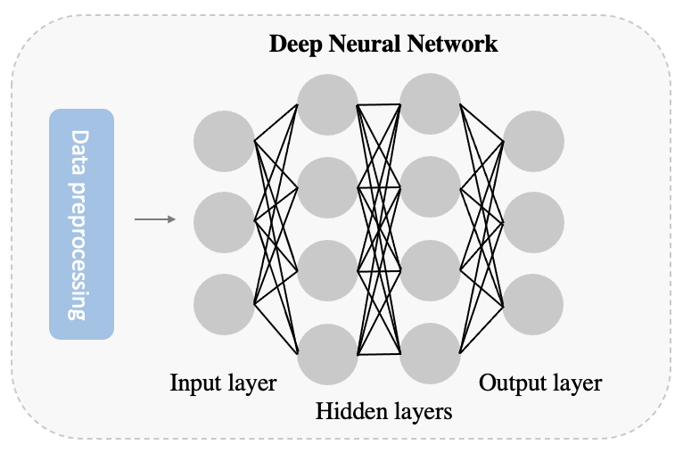
(a) DNN

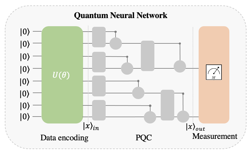
(b) QNN

Figure 1: The structures of DNN and QNN.

With advancements in quantum devices and simulators, quantum machine learning (QML) Schuld & Petruccione (2018) has gained attention by combining machine learning with quantum computing to enhance traditional machine learning algorithms, including clustering Maier et al. (2004), $k$-nearest neighbor ($k$-NN) Dang et al. (2018), support-vector machine (SVM) Rebentrost et al. (2013), principal component analysis (PCA) Cong & Duan (2015), and generative models Gao et al. (2018). Inspired by classical Deep Neural Networks (DNNs) LeCun et al. (1998a); He et al. (2015), Quantum Neural Networks (QNNs) have emerged as a promising branch of QML, capable of processing both classical and quantum data in fields like image classification Benedetti et al. (2019). The core of QNNs is parameterized quantum circuits (PQCs), composed of fixed gates with learnable parameters, making them suitable for optimization tasks like classification. Typically, QNNs consist of three parts: data encoding, parametric circuit, and measurement layers, as shown in Figure 1(b).

While the design of QNN structures is still evolving, many variants Cong et al. (2018); Mitarai et al. (2018); Schuld et al. (2018); Hur et al. (2021); Shi et al. (2023); Henderson et al. (2019); Alam et al. (2021); Li et al. (2022a); Fan et al. (2023) have been proposed. Current QNNs can be generally divided into two categories: pure-quantum models and classical-quantum hybrid models. The pure-quantum models Cong et al. (2018); Mitarai et al. (2018); Schuld et al. (2018); Hur et al. (2021) consist entirely of quantum circuits, while hybrid models Shi et al. (2023); Li et al. (2022a); Alam et al. (2021) integrate QNNs as a quantum layer into classical convolutional neural networks (CNNs). Due to the current limitations of quantum devices in the noisy intermediate-scale quantum (NISQ) era, hybrid models rely primarily on classical components, while pure-quantum models hold more potential as quantum hardware advances. Pure-quantum models can be further categorized by the role of quantum circuits: circuit-body QNNs, which use medium-sized quantum circuits (e.g., eight qubits) to process entire inputs Mitarai et al. (2018); Schuld et al. (2018); Cong et al. (2018); Hur et al. (2021), and quantum kernel-based QNNs, which use smaller circuits (e.g., two qubits) as kernels that slide over data regions to extract features Henderson et al. (2019); Fan et al. (2023), similar to convolutional kernels in DNNs. This paper focuses on circuit-body QNNs.

Although QNNs and DNNs share similarities in their training processes, key differences exist. First, QNNs require classical data encoded into quantum states before gate operations, while DNNs do not need such preprocessing. Second, in QNNs, only the rotation gate angles are adjustable compared to the many parameters in DNNs. Finally, QNN nonlinearity is introduced by quantum measurements rather than activation functions like ReLU Nair & Hinton (2010). These structural differences lead to different solution spaces, making DNN testing techniques inapplicable to QNNs.

3 Coverage criteria for Testing Quantum Neural Networks

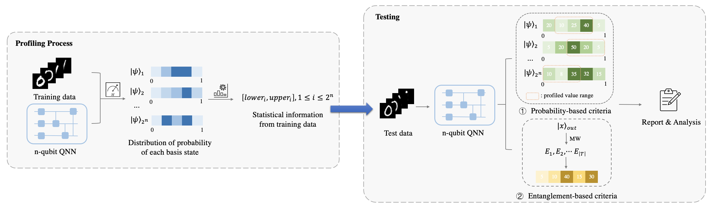
Figure 2: The Workflow of QCov. We profile major and corner-case regions of QNNs using training data. QCov evaluates the test suite and analyzes model behaviors based on probability and entanglement at the testing phase.

Several DNN-oriented test coverage criteria Pei et al. (2017); Ma et al. (2018a; 2019); Xie et al. (2022); Sun et al. (2018); Liu et al. (2023) have been proposed to assess test adequacy and detect defects based on neural behaviors and internal relationships of DNNs. However, research on QNN testing techniques is still in its early stages, lacking systematic guidance for analyzing QNN behaviors, especially errors and corner cases. To take the first step towards testing for QNNs, in this section, we draw inspiration from classical DNN coverage criteria Pei et al. (2017); Ma et al. (2018a) and introduce QCov, a set of QNN-specific testing criteria based on two quantum statistics: superposition and entanglement degree of quantum states. These criteria quantify test adequacy and optimize the detection of unusual behaviors across multiple granularities. To ensure transferability across datasets and circuit designs in different ML tasks, the criteria are designed to be simple to execute while accurately representing the states of quantum systems. Figure 2 shows the overall workflow of QCov.

3.1 Probability-based Coverage Criteria

The probability amplitudes of basis states are fundamental to describing a qubit’s superposition. The output state of a quantum circuit is influenced by both the input state and the operations of quantum gates. In QNNs, the measurement results are widely adopted to represent the model’s outputs, similar to the outputs of neurons in a hidden layer of DNNs.

However, the total number of basis states increases exponentially with the number of qubits, and the probability of each state ranges from 0 to 1 theoretically. This means an astonishing amount of all possible superpositions, making thorough testing challenging. As the model decision logic evolves during training, the probability distribution for each basis state is typically compressed into a smaller range than [0, 1], similar to neuron output boundaries in DNNs Ma et al. (2018a). In this work, we extract probability ranges of each basis state from training data to profile major and corner-case regions in QNNs. Inputs with a similar distribution to training data will have probabilities mostly located in the major regions, while corner-case regions are less frequently explored.

Let $\mathcal{S}=\{s_{1},s_{2},\ldots,s_{2^{n}}\}$ denote the set of basis states, and $\mathcal{T}=\{x_{1},x_{2},\ldots,x_{t}\}$ denote the test suite, where $n$ is the number of qubits and $t$ is the suite size. After analyzing the training dataset, the lower and upper boundaries of the probability for each basis state are derived, denoted as $lower$ and $upper$. During the evaluation, $P(s,x)$ represents the measured probability of basis state $s$ under input $x$.

3.1.1 $k$-cell State Coverage

Since the probability range of each basis state is continuous, we discretize it into finite intervals for quantification. Specifically, for basis state $s$, its probability range $[lower,upper]$ is derived from training data. We refer to this range as the major region of $s$ and divide it into $k$ equal cells, denoted as $\mathcal{C}^{s}=\{c_{1}^{s},c_{2}^{s},\ldots,c_{k}^{s}\}$, where $c_{i}^{s}$ represents the $i$-th sub-range (cell). If $P(s,x)\in c_{i}^{s}$, we consider this cell covered by input $x$. $k$-cell State Coverage (KSC) is defined as the ratio of the number of cells covered by the test suite $\mathcal{T}$ to the total number of cells:

$$KSC(\mathcal{T},k)=\frac{\sum_{s\in\mathcal{S}}|\{c_{i}^{s}\mid\exists{x}\in\mathcal{T},P(s,x)\in c_{i}^{s}\}|}{k*|S|}$$ (2)

KSC reflects how adequately the test suite covers major-region cells, providing a measure of test adequacy in covering the primary behaviors of QNNs.

3.1.2 State Corner Coverage

The corner-case regions of a basis state are those outside the major region, i.e., $(-\infty,lower)\vee(upper,+\infty)$. If a test case follows a distribution similar to the training data, it may cover only a small portion of the corner-case regions. However, it is essential to explore these regions thoroughly, as they may reveal hidden erroneous behaviors Ma et al. (2018a). To quantify the coverage of these regions, we propose State Corner Coverage (SCC), which counts the number of corner regions covered by the test suite. We consider both the lower and upper regions and compute SCC as:

$$SCC(\mathcal{T})=\frac{|\{s\in\mathcal{S}\mid\exists{x}\in\mathcal{T},P(s,x)\in(-\infty,lower)\}|+|\{s\in\mathcal{S}\mid\exists{x}\in\mathcal{T},P(s,x)\in(upper,+\infty)\}|}{2*|S|}$$ (3)

Intuitively, a higher SCC indicates that more previously uncovered regions (relative to the training data) have been explored. This increases the likelihood of detecting potential defects, including adversarial anomalies Lu et al. (2019) and Out-Of-Distribution (OOD) data Liu et al. (2023).

3.1.3 Top-$k$ State Coverage

At the evaluation step, basis states with the largest k probabilities are closely related to the model’s final outputs; we refer to these states as the Top-$k$ States. Besides the statistical information provided by KSC and SCC for individual states, we aim to highlight the comparative relationships between states. To this end, we define Top-$k$ State Coverage (TSC), which measures how many states have once been most influential for some input. TSC is calculated as the ratio of top-$k$ states to the total number of basis states:

$$TSC(\mathcal{T},k)=\frac{|\{s\in\mathcal{S}\mid\exists{x}\in\mathcal{T},s\in top_{k}(x)\}|}{|S|}$$ (4)

For two similarly distributed inputs, their top states are likely to overlap, leading to similar model decisions. To thoroughly test a QNN, the top states produced by the test suite should be as diverse as possible.

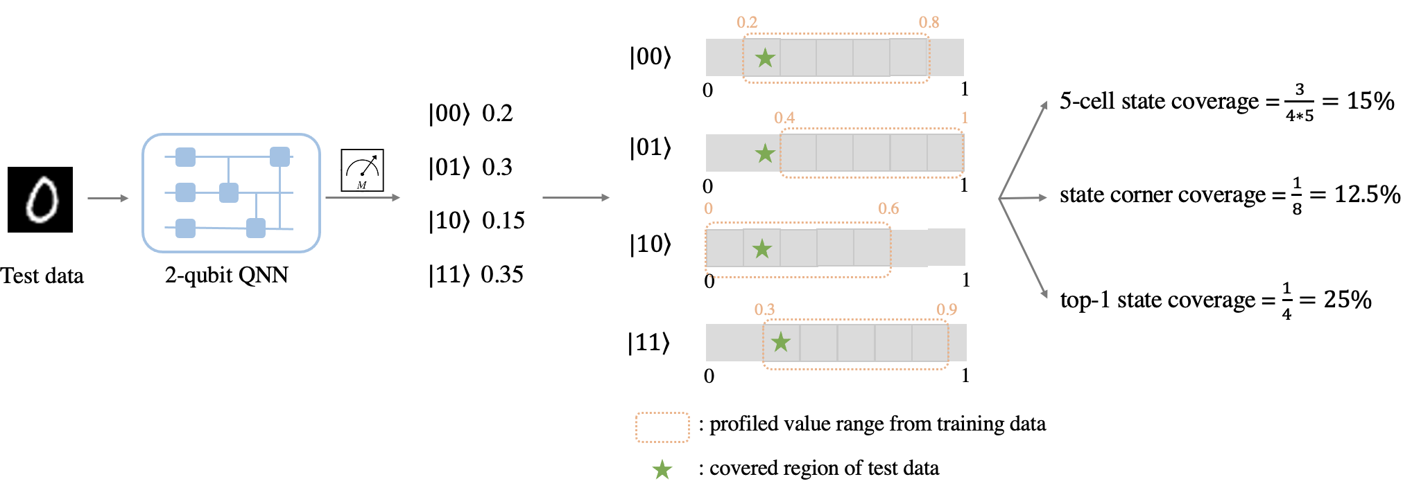
(a) Probability-based criteria

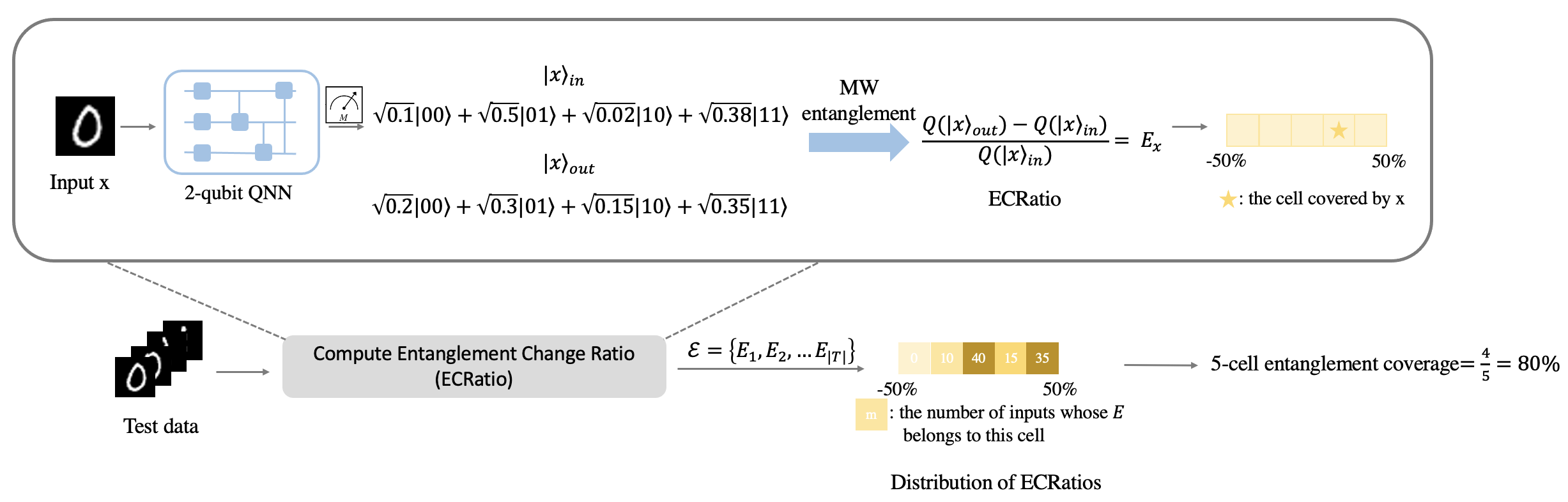
(b) Entanglement-based criterion

Figure 3: Examples of calculation of QCov.

Example 1.

We present an example of computing these criteria in Figure 3(a). Suppose a QNN contains two qubits and four basis states: $|00\rangle$, $|01\rangle$, $|10\rangle$, and $|11\rangle$. The probability range for each basis state, profiled from training data, is divided into five cells (e.g., [0.2, 0.8] for $|00\rangle$, with each cell length being 0.6/5=0.12). Given an input with output probabilities as (0.2, 0.3, 0.15, 0.35), it covers the first cell for $|00\rangle$, the second cell for $|10\rangle$, and the first cell for $|11\rangle$. The 5-KSC is thus 15%. For $|01\rangle$, 0.3 is in its lower region, making the SCC 12.5%. Although an input has only one top-1 state, always yielding a top-1 coverage of 25%, this criterion increases as more test inputs are aggregated.

3.2 Entanglement-based Coverage Criteria

In addition to fine-grained predictive information collected from individual basis states, quantum entanglement is another critical property in quantum computing. It focuses on the correlations between multiple qubits. In QNNs, complex entanglement is usually generated through controlled gates, allowing qubits to interact and influence subsequent quantum states jointly. This enables QNNs to learn feature correlations more effectively, with model performance linked to its entanglement capability Shi et al. (2024); Hur et al. (2021); Shi et al. (2023); Li et al. (2022b). We define an entanglement-based criterion called $k$-cell Entanglement Coverage (KEC) to evaluate model behaviors from the entanglement perspective. The calculation of KEC involves three steps: measuring the entanglement degree, computing the entanglement change ratio (ECRatio), and obtaining KEC.

The first step is to evaluate the entanglement adequacy of a given quantum state. For scalability and computational simplicity, we adopt the Meyer-Wallach (MW) entanglement measure Meyer & Wallach (2001), which quantifies the average entanglement between one qubit and the rest of the system. The measure $\mathcal{Q}$ is defined for a n-qubit quantum state $|\phi\rangle$ in Hilbert space $\mathcal{H}=(\mathbb{C}^{2})^{\otimes n}$. For qubit $i$ ($1\leq i\leq n$), the reduced density matrix $\rho_{i}$ is obtained by tracing out other qubits. The linear entropy $S_{i}$ is then used to quantify the entanglement for each qubit, where $Tr(\rho_{i}^{2})$ is the purity of $\rho_{i}$, and a higher purity indicates lower entanglement. Finally, $\mathcal{Q}(|\phi\rangle)$ is the average linear entropy across all qubits, ranging from 0 to 1, where 1 indicates maximal entanglement:

$$\rho_{i}=Tr_{all\ except\ i}(|\phi\rangle\langle\phi|),S_{i}=2(1-Tr(\rho_{i}^{2}))$$ (5)

$$\mathcal{Q}(|\phi\rangle)=\frac{1}{n}\sum_{i=1}^{n}S_{i}=\frac{2}{n}\sum_{i=1}^{n}(1-Tr(\rho_{i}^{2}))$$ (6)

To represent the runtime changes of input $x$ in entanglement through a QNN, similar to Shi et al. (2024), we adopt the difference between the entanglement of the input and output states, $\mathcal{Q}(|x\rangle_{out})-\mathcal{Q}(|x\rangle_{in})$.

We observed that the entanglement change is input-specific, meaning values from different inputs are not directly comparable. This is due to the fact that the input quantum state is encoded uniquely for each input. To alleviate this impact, we further compute a metric called Entanglement Change Ratio (ECRatio) to measure the relative change in qubit entanglement after an input passes through a QNN:

$$E_{x}=\frac{\mathcal{Q}(|x\rangle_{out})-\mathcal{Q}(|x\rangle_{in})}{\mathcal{Q}(|x\rangle_{in})}$$ (7)

Due to the poor comparability across inputs, we use a fixed range for ECRatio, e.g., [-50%, 50%], instead of profiling training data. The lower bound is negative since the output entanglement is not necessarily greater than the input.

Similar to KSC, the range $[lower,upper]$ is divided into $k$ equal cells $\mathcal{C}=\{c_{1},c_{2},\ldots,c_{k}\}$. A cell $c_{i}$, scaled as $[lower+(i-1)*\frac{upper-lower}{k},lower+i*\frac{upper-lower}{k}]$, is covered by input $x$ if $x$’s ECRatio is located in $c_{i}$. KEC is defined as the percentage of covered cells:

$$KEC(\mathcal{T},k)=\frac{|\{c_{i}\mid\exists{x}\in\mathcal{T},E_{x}\in c_{i}\}|}{k}$$ (8)

Although the boundary between major and corner-case regions is not clearly defined due to the fixed range, a more diverse test suite should contribute to a higher KEC, as discussed in Section 4.2.1.

Example 2.

To illustrate the KEC calculation process, we present a simple example in Figure 3(b). Given a test sample, its input and output states are measured, and the ECRatio is calculated by 7, covering one cell in the range. This process is repeated for each sample in $\mathcal{T}$. Ultimately, $\mathcal{T}$ covers 4 out of 5 cells, resulting in a 5-KEC of 80%.

4 Experiment

We implement QCov using Pytorch 2.1.2 Paszke et al. (2019) and PennyLane 0.32.0 Bergholm et al. (2018) and evaluate its effectiveness and usefulness in this section. In particular, we address the following research questions:

• RQ1: What is the relationship between different coverage criteria and test input diversity?

• RQ2: How effective are the proposed coverage criteria in identifying QNN defects?

• RQ3: Can QCov guide fuzz testing to retain fault-prone seeds and uncover more defects in QNNs?

• RQ4: How efficient is the computation of QCov?

4.1 Evaluation Setup

Table 1: Dataset and QNN architectures

Dataset	Task	Target classes	QNN	#parameter	Acc (%)
MNIST	Binary classification	digits 0 and 1	QCL	150	100.0
			CCQC	260	99.76
			QCNN	229	99.52
			HCQC_TTN	20	97.87
			HCQC_15	40	98.82
			HCQC_SO4	60	95.04
			HCQC_6	100	94.33
			HCQC_SU4	150	97.63
	Ternary classification	digits 2, 4 and 6	QCL	150	88.02
		digits 0, 1 and 2	CCQC	260	92.85
		digits 3, 7 and 9	QCNN	229	85.86
FashionMNIST	Binary classification	T-shirt and Trouser	QCL	150	92.5
			CCQC	260	94.4
			QCNN	229	93.25
			HCQC_TTN	20	88.75
			HCQC_15	40	91.75
			HCQC_SO4	60	92.25
			HCQC_6	100	93.0
			HCQC_SU4	150	92.25

4.1.1 Datasets

The MNIST dataset LeCun et al. (1998b), widely used in machine learning, consists of 70,000 grayscale images (0-9 digits) with $28\times 28$ pixels. It is split into 60,000 training images and 10,000 test images. The FashionMNIST dataset Xiao et al. (2017), a more complex alternative to MNIST, has a similar structure but contains ten categories of fashion articles.

Following previous work in image classification Hur et al. (2021); Shi et al. (2024), we implement binary and ternary classification on MNIST and binary classification on FashionMNIST. The detailed settings are listed in Table 1. Note that ternary classification is not included in HCQC Hur et al. (2021), which is designed for binary classification with one qubit as output. Consistent with prior research on QNNs Alam et al. (2021); Hur et al. (2021); Li et al. (2022a), the training and test dataset sizes are reduced to 20% due to the computational limitations of quantum simulators, resulting in 1200 training samples and 200 test samples per class. To profile QNNs and gather statistical information for the criteria, we sample 100 random images from each class, considering the smaller data size and time constraints.

4.1.2 QNN Architectures

• Quantum Circuit Learning (QCL) Mitarai et al. (2018) is a classical-quantum hybrid network designed for NISQ devices. It approximates nonlinear functions and solves machine learning tasks through iterative optimization of parameters.

• Circuit-centric Quantum Classifiers (CCQC) Schuld et al. (2018) is a low-depth quantum circuit with strong entangling power and good resilience to noise. The model consists of parameterized single and controlled gates designed to capture short and long-range correlations in input data.

• Quantum Convolutional Neural Network (QCNN) Cong et al. (2018) is a hierarchical quantum network motivated by classical CNNs, with convolutional, pooling and fully connected layers implemented by quantum circuits. Nonlinearities are introduced by measuring a subset of qubits in pooling layers to reduce freedom degrees.

• Hierarchical Circuit Quantum Classifier (HCQC) Hur et al. (2021) is another hierarchical network that reduces degrees of freedom as circuits deepen. HCQC traces out qubits through controlled gates and stacks invariant ansatzs translationally to build convolutional and pooling layers. This flexible architecture can be scaled using different two-qubit ansatzs. Five ansatzes are used in our experiments: U_TTN, U_15, U_SO4, U_6, and U_SU4, with 2, 4, 6, 10, and 15 learnable parameters, respectively.

4.1.3 Data Encoding

To adapt classical data for quantum computing, quantum data encoding is required to transform classical data into corresponding quantum states before executing QML tasks Hur et al. (2021). This is achieved by applying a unitary transformation $U(x):\mathcal{R}\mapsto\mathcal{H}$, where $\mathcal{R}$ is n-dimensional Euclidean space and $\mathcal{H}$ is a $2^{n}$-dimensional Hilbert space. We use a widely adopted Amplitude Encoding strategy Wiebe et al. (2012), which represents exponential classical features by encoding normalized input features as the probability amplitudes of basis states. For an input $x$ with $N$ dimensions, it is transformed into a n-qubit quantum state ($N=2^{n}$) as $U(x):x\mapsto\sum_{i=1}^{2^{n}}|i\rangle$, where $|i\rangle$ is the $i$-th computational basis state. Considering the image size, we use a 10-qubit circuit. The extra 240 $(2^{10}-28\times 28)$ amplitudes are set to 0, and the 1024 features are normalized to meet the constraint that the sum of squares equals one.

4.1.4 Adversarial Test Input Generation

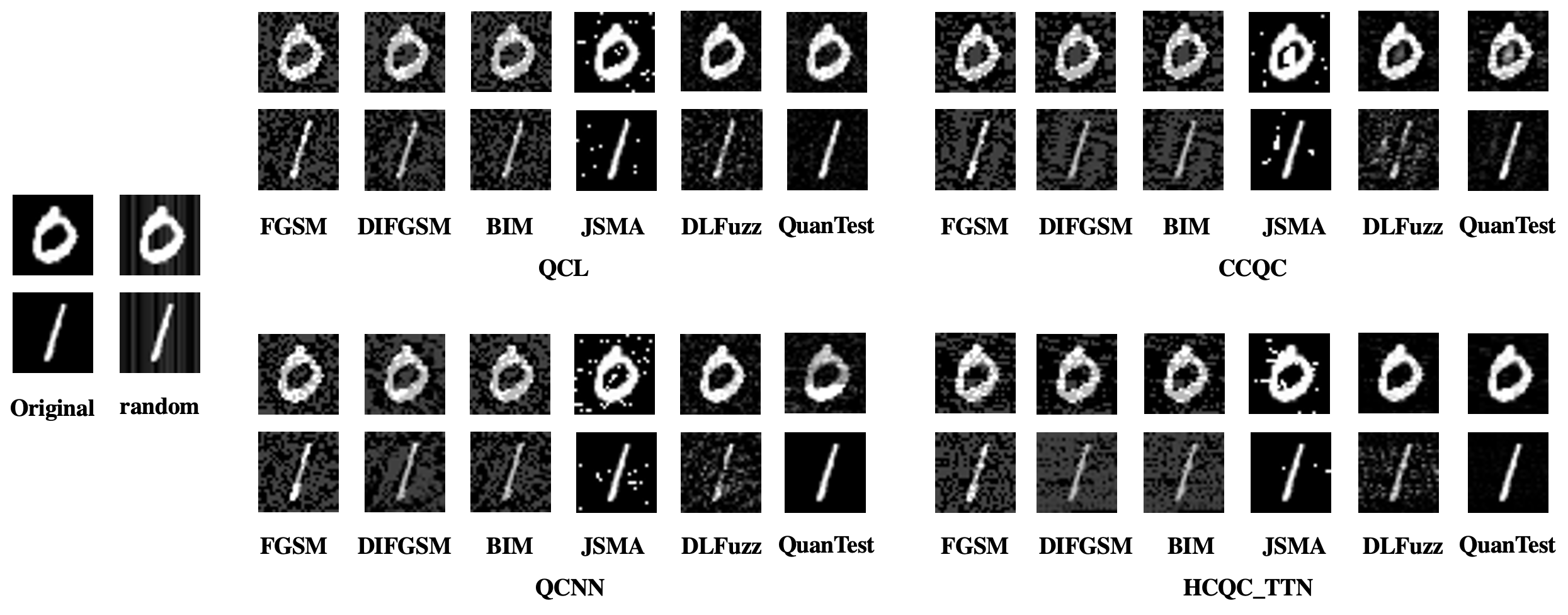
Figure 4: Examples of generated adversarial test inputs. Each attack is data- and model-dependent.

In addition to the original test data, we generate six types of adversarial test data using FGSM Goodfellow et al. (2014), DIFGSM Xie et al. (2018), BIM Kurakin et al. (2016), JSMA Papernot et al. (2015), DLFuzz Guo et al. (2018), and QuanTest Shi et al. (2024). We apply these algorithms to generate adversarial versions of each test case for each QNN and combine them with the original data. Due to time constraints, we select 50 seed inputs per class (100 in total) for each setting. This allows for a comparative study of how effectively our criteria detect abnormal test cases.

• FGSM (Fast Gradient Sign Method)Goodfellow et al. (2014) is a white-box, single-step attack that generates adversarial inputs by adding a gradient sign to the original input.

• DIFGSM (DI2-FGSM)Xie et al. (2018) enhances FGSM’s transferability across networks by applying random transformations to inputs at each iteration.

• BIM (iterative-FGSM)Kurakin et al. (2016) applies adversarial perturbation iteratively with a small step size, keeping the perturbation within a defined epsilon-neighborhood.

• JSMA (Jacobian Saliency Map Attack)Papernot et al. (2015) exploits forward derivatives to create adversarial saliency maps, iteratively modifying features until misclassification occurs.

• DLFuzzGuo et al. (2018) mutates inputs to maximize the difference between the loss of the original class and other classes via gradient ascent.

• QuanTestShi et al. (2024) generates adversarial inputs for QNNs by optimizing entanglement sufficiency to induce incorrect behaviors. The perturbation is applied directly to the input state vector.

Aside from QuanTest, the other five adversarial strategies were originally designed for DL systems. Since they rely on gradients of specific loss functions, we adapted them following Lu et al. (2019) to handle QNNs, where gradients are computed using the parameter shift rule Banchi & Crooks (2020). Figure 4 shows examples of adversarial inputs. Inputs generated by JSMA and QuanTest exhibit better visual quality with less noise, demonstrating more advanced attack stealthiness than other methods. Given a high attack success rate, the similarity between the original input and its adversarial counterpart is crucial for attackers. Effective testing criteria should be able to capture various adversarial inputs.

Table 2: Parameter settings for QCov

Criteria		Parameter Settings
Probability-based criteria	$k$-cell State Coverage (KSC)	$k$=100	$k$=500
	State Corner Coverage (SCC)	LB=$l$, UB=$u$	LB=$l-\sigma$, UB=$u+\sigma$
	Top-$k$ State Coverage (TSC)	top-$k$=1	top-$k$=2
Entanglement-based criterion	$k$-cell Entanglement Coverage (KEC)	$k$=100	$k$=500

4.1.5 Parameter Settings for Criteria

Table 2 provides the detailed parameter settings for QCov. For probability-based criteria, $k$ represents the total number of cells within a given range, while $l$ and $u$ are the lower and upper probability boundaries of each state obtained from the training data. $\sigma$ is the standard deviation of each state’s probability. To evaluate the criteria more thoroughly, we tighten corner-case regions by decreasing the LowerBoundary (LB) and increasing the UpperBoundary (UB), with an additional setting of LB=$l-\sigma$ and UB=$u+\sigma$. For the entanglement-based criterion, $k$ is the number of cells into which the range $[-50\%,50\%]$ is split.

4.2 Experimental Results

4.2.1 RQ1: Relationship with input diversity

Table 3: Coverage results of QCov on MNIST under two sampling strategies (%)

QNN	Sampling strategy		Criteria
			KSC ($k$=100)	CSC ($l$, $u$)	TSC (top-$k$=1)	KEC ($k$=500)
QCL		from 1 class	57.48	48.63	3.32	17.6
	source classes	from 2 classes	59.79	54.1	4.1	18.0
	suite sizes	50 per class	45.72	36.28	2.64	12.4
		100 per class	59.79	54.1	4.1	18.0
CCQC		from 1 class	56.38	49.51	2.44	13.8
	source classes	from 2 classes	58.34	53.91	2.44	16.6
	suite sizes	50 per class	44.54	38.43	1.76	11.8
		100 per class	58.34	53.91	2.44	16.6
QCNN		from 1 class	57.54	48.97	2.73	15.4
	source classes	from 2 classes	59.19	52.1	2.84	17.6
	suite sizes	50 per class	45.39	34.37	1.66	12.4
		100 per class	59.19	52.1	2.84	17.6
HCQC_TTN		from 1 class	44.14	46.04	0.59	8.8
	source classes	from 2 classes	45.19	53.42	1.76	10.8
	suite sizes	50 per class	33.07	35.3	1.27	8.6
		100 per class	45.19	53.42	1.76	10.8
HCQC_15		from 1 class	47.08	50.39	2.15	8.8
	source classes	from 2 classes	48.57	52.98	2.64	13.8
	suite sizes	50 per class	35.95	37.59	1.76	10.6
		100 per class	48.57	52.98	2.64	13.8
HCQC_SO4		from 1 class	46.37	50.78	0.78	10.2
	source classes	from 2 classes	49.29	53.03	1.76	11.6
	suite sizes	50 per class	36.43	37.06	0.97	9.2
		100 per class	49.29	53.03	1.76	11.6
HCQC_6		from 1 class	57.11	48.97	2.54	9.0
	source classes	from 2 classes	59.31	54.1	2.93	11.2
	suite sizes	50 per class	45.35	38.39	2.15	8.0
		100 per class	59.31	54.1	2.93	11.2
HCQC_SU4		from 1 class	53.06	47.12	1.86	8.0
	source classes	from 2 classes	55.11	54.39	2.64	13.8
	suite sizes	50 per class	42.11	38.28	1.95	10.2
		100 per class	55.11	54.39	2.64	13.8
QCL (3)		from 1 class	59.95	46.34	8.11	20.6
		from 2 classes	61.69	50.32	10.13	21.4
	source classes	from 3 classes	61.7	50.78	10.64	22.0
	suite sizes	50 per class	50.21	35.11	7.13	17.6
		100 per class	61.7	50.78	10.64	22.0
CCQC (3)		from 1 class	56.17	43.9	2.34	12.0
		from 2 classes	58.98	49.95	3.22	19.2
	source classes	from 3 classes	60.08	53.86	5.08	22.4
	suite sizes	50 per class	47.95	37.35	3.71	16.6
		100 per class	60.08	53.86	5.08	22.4
QCNN (3)		from 1 class	46.97	44.09	1.07	13.0
		from 2 classes	51.34	52.83	1.36	14.0
	source classes	from 3 classes	52.03	51.51	1.37	13.2
	suite sizes	50 per class	41.52	37.16	0.98	11.0
		100 per class	52.03	51.51	1.37	13.2

Table 4: Coverage results of QCov on FashionMNIST under two sampling strategies (%)

QNN	Sampling strategy		Criteria
			KSC ($k$=100)	CSC ($l$, $u$)	TSC (top-$k$=1)	KEC ($k$=500)
QCL		from 1 class	56.27	53.27	1.86	7.4
	source classes	from 2 classes	60.84	54.59	2.34	16.6
	suite sizes	50 per class	46.59	27.73	1.27	8.4
		100 per class	60.84	54.59	2.34	16.6
CCQC		from 1 class	55.98	73.83	0.88	19.4
	source classes	from 2 classes	60.26	73.88	1.27	24.8
	suite sizes	50 per class	42.05	32.47	1.17	15.8
		100 per class	60.26	73.88	1.27	24.8
QCNN		from 1 class	47.78	51.27	0.49	20
	source classes	from 2 classes	55.15	55.13	0.68	23.2
	suite sizes	50 per class	41.86	32.28	0.49	14.4
		100 per class	55.15	55.13	0.68	23.2
HCQC_TTN		from 1 class	37.73	52.83	0.39	14.8
	source classes	from 2 classes	44.58	55.18	0.49	16
	suite sizes	50 per class	33.02	32.91	0.39	10.4
		100 per class	44.58	55.18	0.49	16
HCQC_15		from 1 class	41.41	52.93	0.49	14.2
	source classes	from 2 classes	47.92	53.61	0.59	17
	suite sizes	50 per class	35.61	32.03	0.2	11.8
		100 per class	47.92	53.61	0.59	17
HCQC_SO4		from 1 class	45.54	53.81	0.68	16.8
	source classes	from 2 classes	50.47	54.88	0.78	19.2
	suite sizes	50 per class	37.97	32.32	0.49	14
		100 per class	50.47	54.88	0.78	19.2
HCQC_6		from 1 class	52.86	53.13	0.49	14.2
	source classes	from 2 classes	58.76	56.59	0.68	15.8
	suite sizes	50 per class	44.87	30.22	0.59	11.6
		100 per class	58.76	56.59	0.68	15.8
HCQC_SU4		from 1 class	50.82	53.66	0.29	16
	source classes	from 2 classes	56.61	56.44	0.29	20
	suite sizes	50 per class	43.23	30.91	0.2	14.2
		100 per class	56.61	56.44	0.29	20

Test diversity is crucial for assessing test case quality in both traditional software and DL testing. A test suite with limited categories or small size may fail to uncover various defects in QNNs. Effective criteria should be sensitive to test diversity, meaning more diverse inputs should cover more internal behaviors and result in higher coverage scores. We evaluate the relationship between the proposed criteria and test diversity using two sampling strategies. The first strategy collects inputs from either a single class or multiple classes, as inputs from more classes should increase diversity. The second strategy varies the suite size by increasing the sample number per class (e.g., 50 or 100 per class) to simulate more diverse test cases. To ensure fairness, all test suites have the same size: 200 for binary classification and 300 for ternary classification. We calculate the coverage for all settings, with results shown in Tables 3 and 4.

The results show that both probability-based and entanglement-based criteria increase with test diversity, demonstrating a positive correlation between QCov and test diversity. Key findings include:

(1) For probability-based criteria on MNIST, the correlation is stronger in ternary classification than in binary classification. Ternary classification involves measurement results of three qubits, leading to more output distributions and less overlap between outputs of different inputs. New inputs generated by both strategies often produce previously unseen outputs, resulting in higher coverage scores.

(2) Probability-based criteria increase more with the second strategy (increasing suite size) than with the first strategy (diversifying source classes). For instance, on MNIST with QCL, KSC ($k$=100) increases by 131% (from 45.72% to 59.79%) in the second strategy, compared to 104% (from 57.48% to 59.79%) in the first. This is because, while the first strategy adds class diversity, it also drops some input information under the constraint of the same suite size, limiting coverage improvement.

(3) KEC generally improves with both strategies. For example, on CCQC and MNIST, KEC ($k$=500) increases by 116% (from 13.8% to 16.6%) and 141% (from 11.8% to 16.6%), respectively, as new inputs induce more entanglement by encoding different states.

(4) In some cases, KEC shows a negative correlation with diversity. For example, on MNIST and QCNN (ternary classification), inputs from 2 classes (150 per class) yield a higher KEC (14%) than inputs from 3 classes (100 per class, KEC of 13.2%). This may result from dropping 50 inputs from the original two classes, which were more diverse than the added inputs from the new class. However, KEC for 2 and 3 classes is still higher than that for 1 class, indicating an overall positive trend.

(5) Probability-based criteria show a stronger correlation with test diversity than entanglement-based criteria, as the former provides a more fine-grained analysis of each basis state, while the latter focuses on the overall system state.

Table 5: Probability-based Coverage results on MNIST and erroneous inputs (%)

Criteria	QNN	Param.	Org.	Org.+Random	Org.+FGSM	Org.+DIFGSM	Org.+BIM	Org.+JSMA	Org.+DLFuzz	Org.+QuanTest
KSC	QCL	$k$=100	45.72	58.42	59.13	58.74	58.76	59.74	58.87	58.74
		$k$=500	16.05	26.84	26.75	26.62	26.52	26.98	26.62	26.61
	CCQC	$k$=100	44.54	56.96	58.43	57.13	57.17	58.73	57.93	57.77
		$k$=500	15.82	26.15	26.42	26.02	25.98	26.33	26.08	25.89
	QCNN	$k$=100	45.39	57.97	59.33	58.3	58.3	59.21	58.68	54.65
		$k$=500	16.0	26.51	26.64	26.47	26.3	26.78	26.4	23.4
	HCQC_TTN	$k$=100	33.07	43.56	45.7	42.9	43.45	45.27	44.1	43.77
		$k$=500	12.25	19.3	19.6	18.34	18.52	19.72	19.06	18.99
	HCQC_15	$k$=100	35.95	46.88	48.0	46.87	47.19	48.28	47.97	47.74
		$k$=500	13.19	20.94	20.77	20.3	20.31	21.14	20.78	20.85
	HCQC_SO4	$k$=100	36.43	46.49	46.79	45.48	45.65	49.18	47.93	48.29
		$k$=500	13.32	20.85	20.34	19.87	19.8	21.49	20.87	21.11
	HCQC_6	$k$=100	45.35	56.65	57.51	56.04	56.07	58.45	58.26	57.03
		$k$=500	15.96	26.08	25.97	25.31	25.36	26.3	26.33	25.0
	HCQC_SU4	$k$=100	42.11	53.93	55.85	54.06	54.55	55.44	54.93	54.15
		$k$=500	15.27	24.9	25.1	24.39	24.43	24.64	24.8	24.15
	QCL (3)*	$k$=100	50.21	59.9	61.41	60.96	61.17	61.23	61.38	59.46
		$k$=500	21.46	32.82	32.89	32.7	32.64	32.71	33.08	31.58
	CCQC (3)*	$k$=100	47.95	57.95	60.08	58.46	58.54	59.97	59.67	59.42
		$k$=500	20.54	31.01	31.65	30.88	30.94	31.41	31.42	31.2
	QCNN (3)*	$k$=100	41.52	50.06	53.24	50.57	52.02	53.15	51.94	46.63
		$k$=500	18.58	27.08	28.04	26.95	27.38	27.75	27.46	24.42
SCC	QCL	LB=$l$, UB=$u$	36.28	45.17	55.22	53.76	55.22	53.51	54.79	46.34
		$l-\sigma$, $u+\sigma$	7.13	8.59	16.36	16.06	17.63	13.96	16.65	9.91
	CCQC	LB=$l$, UB=$u$	38.43	47.85	57.03	53.86	54.93	56.15	56.79	50.29
		$l-\sigma$, $u+\sigma$	9.23	10.84	18.99	17.09	17.82	19.48	19.92	14.65
	QCNN	LB=$l$, UB=$u$	34.37	45.36	53.91	50.39	54.15	51.85	52.49	45.95
		$l-\sigma$, $u+\sigma$	6.49	8.79	17.43	13.13	16.94	15.38	17.33	14.11
	HCQC_TTN	LB=$l$, UB=$u$	35.3	46.09	55.66	55.96	56.55	51.86	52.44	44.73
		$l-\sigma$, $u+\sigma$	12.45	14.16	24.61	22.27	23.54	22.17	21.0	14.21
	HCQC_15	LB=$l$, UB=$u$	37.59	47.17	57.76	56.4	57.81	52.78	57.57	50.09
		$l-\sigma$, $u+\sigma$	12.6	14.06	24.9	22.61	24.61	20.46	25.49	18.31
	HCQC_SO4	LB=$l$, UB=$u$	37.06	45.95	57.76	55.22	55.66	54.44	57.03	47.65
		$l-\sigma$, $u+\sigma$	10.93	11.72	20.02	18.6	19.58	20.07	22.46	15.28
	HCQC_6	LB=$l$, UB=$u$	38.39	48.68	57.42	56.93	57.13	54.54	55.96	47.61
		$l-\sigma$, $u+\sigma$	8.98	10.69	17.82	17.58	17.63	18.31	18.6	12.84
	HCQC_SU4	LB=$l$, UB=$u$	38.28	47.41	56.3	55.08	58.89	56.25	56.79	50.05
		$l-\sigma$, $u+\sigma$	13.18	14.94	24.22	21.97	23.88	25.34	24.22	19.04
	QCL (3)*	LB=$l$, UB=$u$	35.11	43.55	53.37	52.34	55.86	48.88	50.98	41.26
		$l-\sigma$, $u+\sigma$	7.18	8.06	16.4	16.5	18.16	11.43	14.94	7.96
	CCQC (3)*	LB=$l$, UB=$u$	37.35	47.17	55.32	53.96	54.83	54.88	53.56	47.51
		$l-\sigma$, $u+\sigma$	10.79	11.72	19.38	18.6	19.09	21.14	18.6	15.53
	QCNN (3)*	LB=$l$, UB=$u$	37.16	44.73	54.59	50.0	56.2	55.08	55.32	43.26
		$l-\sigma$, $u+\sigma$	13.09	13.92	23.0	17.09	23.34	23.0	22.9	15.09
TSC	QCL	top-$k$=1	2.64	3.52	5.67	5.96	6.35	5.86	6.25	3.81
		top-$k$=2	5.96	7.52	9.96	10.55	11.04	10.94	10.55	8.59
	CCQC	top-$k$=1	1.76	1.95	2.25	2.64	2.54	3.12	2.25	2.25
		top-$k$=2	2.73	2.93	3.61	4.0	4.1	4.39	3.71	3.71
	QCNN	top-$k$=1	1.66	1.86	4.1	3.12	3.71	3.61	3.81	3.02
		top-$k$=2	3.42	3.81	6.64	5.86	6.54	6.35	6.54	5.37
	HCQC_TTN	top-$k$=1	1.27	1.37	1.27	1.37	1.37	1.76	1.37	1.37
		top-$k$=2	2.15	2.34	2.25	2.64	2.54	2.93	2.25	2.34
	HCQC_15	top-$k$=1	1.76	2.05	3.32	3.42	3.71	3.42	3.32	2.54
		top-$k$=2	3.52	3.71	5.66	5.76	6.05	5.86	5.57	4.49
	HCQC_SO4	top-$k$=1	0.97	0.98	0.98	1.17	1.07	1.76	1.17	1.37
		top-$k$=2	2.44	2.44	2.44	2.64	2.73	3.71	2.54	2.64
	HCQC_6	top-$k$=1	2.15	2.15	2.44	2.73	2.73	2.34	2.34	2.25
		top-$k$=2	3.13	3.22	3.42	3.52	3.61	4.1	3.32	3.32
	HCQC_SU4	top-$k$=1	1.95	2.05	2.05	2.64	2.54	3.12	2.64	2.34
		top-$k$=2	2.93	3.03	3.22	3.9	3.91	4.49	4.1	3.61
	QCL (3)*	top-$k$=1	7.13	8.11	10.94	10.35	11.23	9.57	11.23	8.5
		top-$k$=2	11.62	12.89	17.68	17.09	17.68	17.19	17.48	13.28
	CCQC (3)*	top-$k$=1	3.71	4.0	4.49	4.39	4.39	6.54	4.39	5.18
		top-$k$=2	5.66	5.86	6.54	6.35	6.25	8.69	6.74	6.84
	QCNN (3)*	top-$k$=1	0.98	1.07	1.27	1.17	1.27	1.27	1.37	1.17
		top-$k$=2	1.86	1.95	2.05	2.25	2.34	2.25	2.25	2.15

• model for ternary classification task.

Answer to RQ1: Both probability-based and entanglement-based criteria show a positive correlation with test diversity. This correlation can be influenced by the choice of dataset and model structure.

4.2.2 RQ2: Effectiveness in identifying defects

Table 6: Entanglement-based Coverage Results on MNIST and erroneous inputs (%)

Criteria	QNN	Param.	Org.	Org.+Random	Org.+FGSM	Org.+DIFGSM	Org.+BIM	Org.+JSMA	Org.+DLFuzz	Org.+QuanTest
KEC	QCL	$k$=100	26.0	37.0	35.0	36.0	35.0	29.0	28.0	31.0
		$k$=500	12.4	22.4	21.4	22.0	21.6	17.6	17.2	20.2
	CCQC	$k$=100	20.0	30.0	33.0	44.0	46.0	23.0	27.0	25.0
		$k$=500	11.8	19.0	20.6	25	25.6	14.4	17.0	17.2
	QCNN	$k$=100	23.0	34.0	33.0	39.0	34.0	25.0	28.0	30.0
		$k$=500	12.4	21.6	21.0	23.2	21.0	15.8	17.4	18.0
	HCQC_TTN	$k$=100	12.0	14.0	17.0	16.0	15.0	15.0	22.0	14.0
		$k$=500	8.6	10.6	13.2	11.8	11.8	11.2	14.8	11.4
	HCQC_15	$k$=100	17.0	23.0	23.0	28.99	25	18.0	21.0	20.0
		$k$=500	10.6	16.6	16.8	19.8	18.2	12.4	14.6	13.6
	HCQC_SO4	$k$=100	15.0	20.0	16.0	21.0	18.0	16.0	19.0	17.0
		$k$=500	9.2	14.0	12.2	15.0	13.8	10.6	13.8	11.8
	HCQC_6	$k$=100	14.0	18.0	17.0	20.0	19.0	15.0	17.0	16.0
		$k$=500	8.0	12.2	12.8	13.8	13.2	9.6	10.4	10.0
	HCQC_SU4	$k$=100	17.0	21.0	26.0	36.0	31.0	19.0	22.0	20.0
		$k$=500	10.2	14.6	16.8	20.6	19.8	13.2	14.6	14.0
	QCL (3)	$k$=100	28.0	40.0	36.0	37.0	37.0	32.0	30.0	36.0
		$k$=500	17.6	28.4	26.2	28.0	26.2	22.2	21.4	23.0
	CCQC (3)	$k$=100	29.00	37.0	40.0	47.0	46.0	35.0	31.0	36.0
		$k$=500	16.6	26.4	26.2	30.4	30.6	21.2	20.6	23.4
	QCNN (3)	$k$=100	15.0	26.0	30.0	32.0	30.0	20.0	19.0	22.0
		$k$=500	11.0	20.4	21.0	24.0	23.0	14.0	14.4	14.0

Table 7: Probability-based Coverage results on FashionMNIST and erroneous inputs (%)

Criteria	QNN	Param.	Org.	Org.+Random	Org.+FGSM	Org.+DIFGSM	Org.+BIM	Org.+JSMA	Org.+DLFuzz	Org.+QuanTest
KSC	QCL	$k$=100	46.59	57.87	61.8	59.93	61.46	61.25	60.02	58.45
		$k$=500	16.24	26.98	27.58	27.39	27.37	27.49	27.34	26.89
	CCQC	$k$=100	42.05	52.38	55.55	53.17	53.4	55.87	54.0	53.15
		$k$=500	15.42	24.86	25.67	24.91	24.93	25.52	25.18	24.92
	QCNN	$k$=100	41.86	52.0	55.4	52.84	53.37	55.03	54.07	52.3
		$k$=500	15.39	24.72	25.6	24.82	24.87	25.37	25.12	24.21
	HCQC_TTN	$k$=100	33.02	41.82	45.04	42.34	42.99	42.87	43.45	41.53
		$k$=500	12.49	19.4	19.99	18.94	19.1	19.24	19.66	18.8
	HCQC_15	$k$=100	35.61	44.27	47.65	45.81	46.51	47.43	46.78	46.28
		$k$=500	13.26	20.62	21.13	20.39	20.49	21.26	21.08	20.97
	HCQC_SO4	$k$=100	37.97	46.96	49.91	48.62	48.93	50.28	49.17	48.95
		$k$=500	13.91	21.89	22.22	21.63	21.65	22.54	22.35	22.25
	HCQC_6	$k$=100	44.87	54.79	58.79	58.24	58.2	58.05	57.21	56.49
	HCQC_SU4	$k$=100	43.23	52.9	56.19	54.5	54.87	56.28	55.03	54.32
		$k$=500	15.64	25.27	25.8	25.13	25.22	25.84	25.73	25.19
SCC	QCL	LB=$l$, UB=$u$	27.73	33.2	52.69	43.99	54.59	46.44	46.68	34.57
		$l-\sigma$, $u+\sigma$	3.61	4.1	16.6	9.38	18.26	10.4	12.35	4.79
	CCQC	LB=$l$, UB=$u$	32.47	40.53	53.96	51.46	52.2	51.07	49.76	41.89
		$l-\sigma$, $u+\sigma$	5.62	6.1	16.11	13.09	14.01	16.94	13.23	8.25
	QCNN	LB=$l$, UB=$u$	32.28	40.67	54.2	50.0	52.83	49.66	51.71	38.67
		$l-\sigma$, $u+\sigma$	5.52	6.05	17.77	11.28	15.09	12.74	14.55	7.03
	HCQC_TTN	LB=$l$, UB=$u$	32.91	40.92	54.69	54.93	56.59	48.0	49.51	42.87
		$l-\sigma$, $u+\sigma$	9.28	9.62	20.21	19.14	20.9	16.8	17.38	11.87
	HCQC_15	LB=$l$, UB=$u$	32.03	40.53	58.5	57.08	62.21	48.54	52.25	43.85
		$l-\sigma$, $u+\sigma$	7.57	7.36	23.05	22.85	26.76	15.77	18.6	11.57
	HCQC_SO4	LB=$l$, UB=$u$	32.32	40.72	57.71	57.37	59.38	50.24	50.49	43.41
		$l-\sigma$, $u+\sigma$	6.84	7.37	21.34	21.14	23.54	16.26	18.07	11.18
	HCQC_6	LB=$l$, UB=$u$	30.22	36.77	55.42	59.42	60.89	46.92	45.65	40.53
		$l-\sigma$, $u+\sigma$	5.42	5.71	16.26	19.34	21.24	13.04	11.72	8.3
	HCQC_SU4	LB=$l$, UB=$u$	30.91	37.79	58.5	57.13	58.79	48.44	44.68	39.89
		$l-\sigma$, $u+\sigma$	5.22	5.66	17.68	17.33	20.12	13.48	12.55	8.35
TSC	QCL	top-$k$=1	1.27	1.56	2.34	2.05	2.83	2.15	1.76	1.46
		top-$k$=2	2.34	2.54	4.3	3.71	4.39	3.32	3.52	2.83
	CCQC	top-$k$=1	1.17	1.17	1.37	1.37	1.37	1.17	1.38	1.17
		top-$k$=2	1.27	1.27	1.46	1.46	1.46	1.27	1.46	1.27
	QCNN	top-$k$=1	0.49	0.49	0.78	0.98	0.88	0.78	0.98	0.49
		top-$k$=2	0.78	0.88	1.17	1.17	1.17	0.98	1.17	0.78
	HCQC_TTN	top-$k$=1	0.39	0.39	0.39	0.59	0.59	0.39	0.39	0.39
		top-$k$=2	0.68	0.68	0.88	0.88	0.98	0.68	0.78	0.68
	HCQC_15	top-$k$=1	0.2	0.2	0.29	0.39	0.39	0.2	0.29	0.2
		top-$k$=2	0.39	0.39	0.59	0.88	0.68	0.49	0.59	0.39
	HCQC_SO4	top-$k$=1	0.49	0.49	0.59	0.88	0.98	0.49	0.59	0.49
		top-$k$=2	0.88	0.88	0.88	1.56	1.46	0.88	0.88	0.88
	HCQC_6	top-$k$=1	0.59	0.59	0.78	0.98	0.88	0.68	0.78	0.68
		top-$k$=2	0.98	0.98	1.17	1.76	1.66	0.98	1.17	0.98
	HCQC_SU4	top-$k$=1	0.2	0.2	0.39	0.29	0.29	0.39	0.2	0.2
		top-$k$=2	0.29	0.29	0.49	0.78	0.59	0.49	0.39	0.29

Table 8: Entanglement-based Coverage Results on FashionMNIST and erroneous inputs (%)

Criteria	QNN	Param.	Org.	Org.+Random	Org.+FGSM	Org.+DIFGSM	Org.+BIM	Org.+JSMA	Org.+DLFuzz	Org.+QuanTest
KEC	QCL	$k$=100	24.0	33.0	34.0	33.0	35.0	33.0	33.0	29.0
		$k$=500	8.4	15.2	17.6	14.6	17.6	15.6	14.4	14.6
	CCQC	$k$=100	37.0	38.0	39.0	38.0	38.0	39.0	39.0	39.0
		$k$=500	15.8	21.0	22.8	18.6	18.6	21.8	23.6	22.2
	QCNN	$k$=100	36.0	46.0	45.0	46.0	47.0	44.0	43.0	45.0
		$k$=500	14.4	23.4	24.8	26.0	24.4	22.8	23.4	24.2
	HCQC_TTN	$k$=100	20.0	24.0	29.0	32.0	33.0	21.0	28.0	29.0
		$k$=500	10.4	15.2	19.2	19.0	21.0	13.6	17.2	16.8
	HCQC_15	$k$=100	21.0	26.0	26.0	31.0	31.0	25.0	27.0	30.0
		$k$=500	11.8	17.0	17.6	19.4	19.8	17.4	18.2	18.4
	HCQC_SO4	$k$=100	25.0	32.0	27.0	32.0	33.0	27.0	28.0	28.0
		$k$=500	14.0	21.8	18.6	21.4	21.0	18.2	17.6	18.8
	HCQC_6	$k$=100	22.0	32.0	23.0	29.0	28.0	24.0	24.0	27.0
		$k$=500	11.6	20.2	15.6	18.6	20.8	16.4	17.0	17.4
	HCQC_SU4	$k$=100	27.0	34.0	30.0	40.0	40.0	32.0	32.0	37.0
		$k$=500	14.2	21.8	20.2	23.6	24.2	19.8	20.4	22.2

The coverage results for all combinations of original and generated adversarial inputs are listed in Tables 5, 6, 7, and 8. The coverage generally increases across all criteria when using different generation algorithms compared to the original test suite.

Probability-based criteria. For example, on MNIST with HCQC_15, QuanTest increases 100-KSC from 35.95% to 47.74% (a 32.8% increase), SCC from 37.59% to 50.09% (a 33.3% increase), and 1-TSC from 1.76% to 2.54% (a 44.3% increase). The improvement in both major regions (KSC) and corner-case regions (SCC) indicates that the proposed criteria effectively capture different behaviors between benign and adversarial inputs. This is because, adversarial inputs are designed to trigger underlying defects in QNNs, leading to outputs that deviate from benign inputs and improve coverage scores.

In addition to manually crafted adversarial inputs, we also want to detect potential natural errors using our criteria. To this end, we use random noise from a uniform distribution to generate another set of test suites, some of which are misclassified by the model. As shown in the ”Org.+random” column in Tables 5 and 7, the criteria also show a significant increase, indicating effectiveness in detecting natural errors. Compared to adversarial settings, the increase of SCC under random noise is less pronounced than that of KSC. For example, on FashionMNIST with QCNN, in columns ”Org.”, ”Org.+Random,” and ”Org.+FGSM,” the increase of KSC is close (from 41.86% to 52% and 55.4% respectively). However, the increase of SCC is from 32.28% to 40.67% in Random compared to 54.2% in FGSM. This suggests that natural errors are primarily located in major regions and less frequently in corner-case regions. Additionally, the relatively small increase in TSC, even combined with erroneous inputs, indicates the stability of top-basis states, providing insights into the abstract decision structure of QNNs. Nevertheless, adversarial data still enable exploration of more top-basis states and behaviors in many cases.

Entanglement-based criterion. The increasing trend of KEC is similar to that of probability-based criteria. For example, on FashionMNIST with QCL, BIM increases 500-KEC from 8.4% to 17.6%, a 110% increase. These results reflect the varied ECRatios of adversarial inputs. The generated noise perturbs the input state, activating more diverse activities of controlled gates and producing new output states. To provide a clearer view, Figure 5 shows a heatmap of ECRatios for different test suites, depicting the coverage density of each cell. In many cases, adversarial data show higher ECRatios than original data due to more active basis states, which result from some originally zero-valued amplitudes being converted to non-zero values by adversarial noise, triggering more activities in controlled gates. However, the increase in criteria is smaller on JSMA and QuanTest, as these attacks perturb fewer pixels and produce higher-quality adversarial inputs. Interestingly, natural-error inputs sometimes achieve higher KECs than adversarial inputs. For instance, on MNIST with HCQC_SO4 ($k$=500), ”Org.+random” achieves 14% KEC, compared to 12.2% for ”Org.+FGSM”. This is likely due to more random and larger perturbation regions in natural-error inputs, resulting in more non-zero amplitudes.

While QCov can help identify defects in QNNs, increasing coverage does not necessarily lead to discovering new defects. Similar to DNN testing Wang et al. (2024); Xie et al. (2022), the relationship between model robustness and coverage criteria requires further investigation.

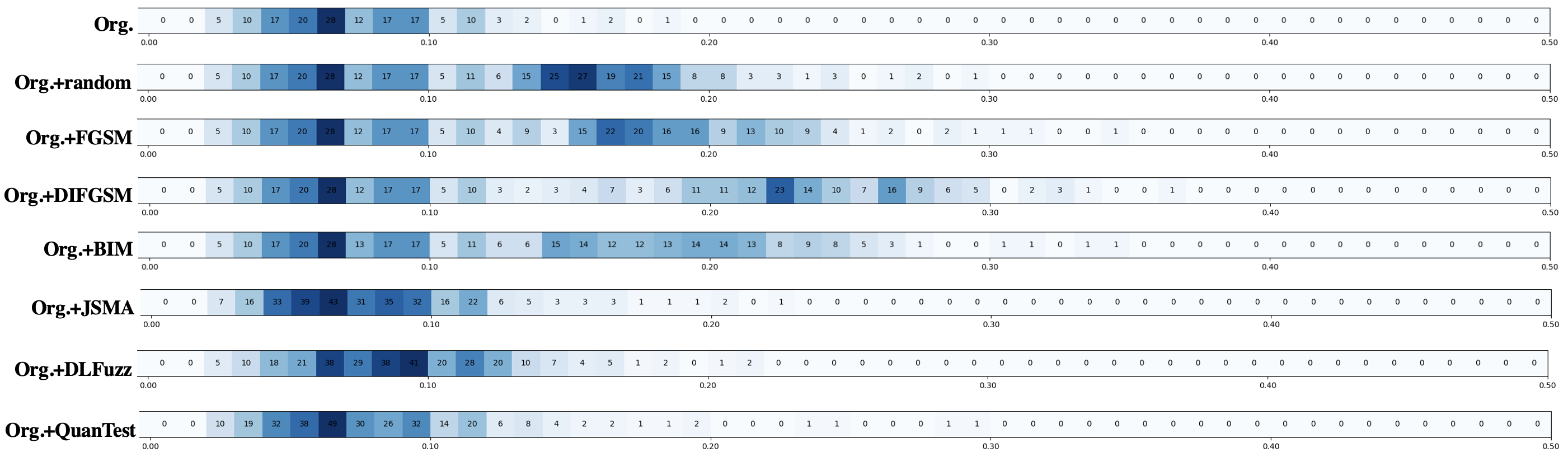
Figure 5: ECRatios of original MNIST test and adversarial inputs under QCNN (ternary classification). For illustration, we only present the right sub-interval [0, 50%] where almost all inputs are located. The number in each cell denotes the number of inputs whose ECRatio belongs to this sub-range.

Answer to RQ2: Overall, QCov demonstrates a strong ability to detect both natural and adversarial errors, effectively distinguishing the model’s behaviors in response to benign and abnormal inputs.

4.2.3 RQ3: Effectiveness in coverage-guided fuzz testing

To demonstrate the usefulness of QCov, we apply it to a practical application: Coverage-Guided Fuzz Testing (CGF). CGF Tian et al. (2017); Xie et al. (2019) explores the input space of models more efficiently by using coverage criteria to guide the fuzzing process. It provides feedback to retain generated seeds that are more likely to trigger misbehaviors in DNNs. Mutation operators generate mutants for testing, and those that increase coverage are enqueued back for further mutation until the budget is exhausted. In this experiment, we integrate QCov into the existing fuzzing framework DeepHunter Xie et al. (2019) to adapt CGF for QNN testing. DeepHunter generates valid, in-distribution transformed images through pixel-level metamorphic mutations, including pixel value and affine transformations. Algorithm 1 summarizes the CGF procedure guided by QCov. The seed queue $Q$ is initialized with $I$, and the defect queue $U$ starts empty. Fuzzing continues until no seeds remain for the mutation (Line 3). At each iteration, a seed $s$ is popped from $Q$ (Line 4), mutated to produce a mutant $m$ (Line 5), and checked for misbehavior. If $m$ triggers misclassification, it is added to the failed set (Line 7). If it passes and increases coverage, it is re-enqueued for further mutation (Line 9). Otherwise, it is discarded.

To conduct a comparative study, we use Random Testing (RT) without coverage guidance Xie et al. (2019) as the baseline and measure Test Success Rate (TSR, i.e., the proportion of misclassified cases generated from initial seeds) Xie et al. (2024). Due to space limitations, we report results for one parameter setting per criterion: $k$=100 for KSC, LB=$l$, UB=$u$ for SCC, top-$k$=1 for TSC, and $k$=500 for KEC. As shown in Figure 6, testing guided by the proposed criteria generates failed test cases more efficiently than random testing across all datasets and models. Compared to RT, the average TSRs of the proposed criteria increase by 110% on MNIST (from 20% to 42%) and by 100% on FashionMNIST (from 19% to 38%), demonstrating QCov’s effectiveness in retaining seeds with the potential to trigger defects.

Algorithm 1 Coverage-guided Fuzz Testing for QNNs

1:Input: $I:$ initial seeds, $QNN:$ target neural network

2:Output: $U:$ failed test cases

3:$U\leftarrow\emptyset$

4:$Q\leftarrow I$

5:while $|Q|>0$ do

6:     $s\leftarrow Q.pop()$

7:     $m\leftarrow Muatator(s)$

8:     if $isFailed(m,QNN)$ then

9:         $U\leftarrow U\cup\{m\}$

10:     else if $covIncrease(m,I\cup U)$ then

11:         $Q\leftarrow Q\cup\{m\}$      

12:return $U$

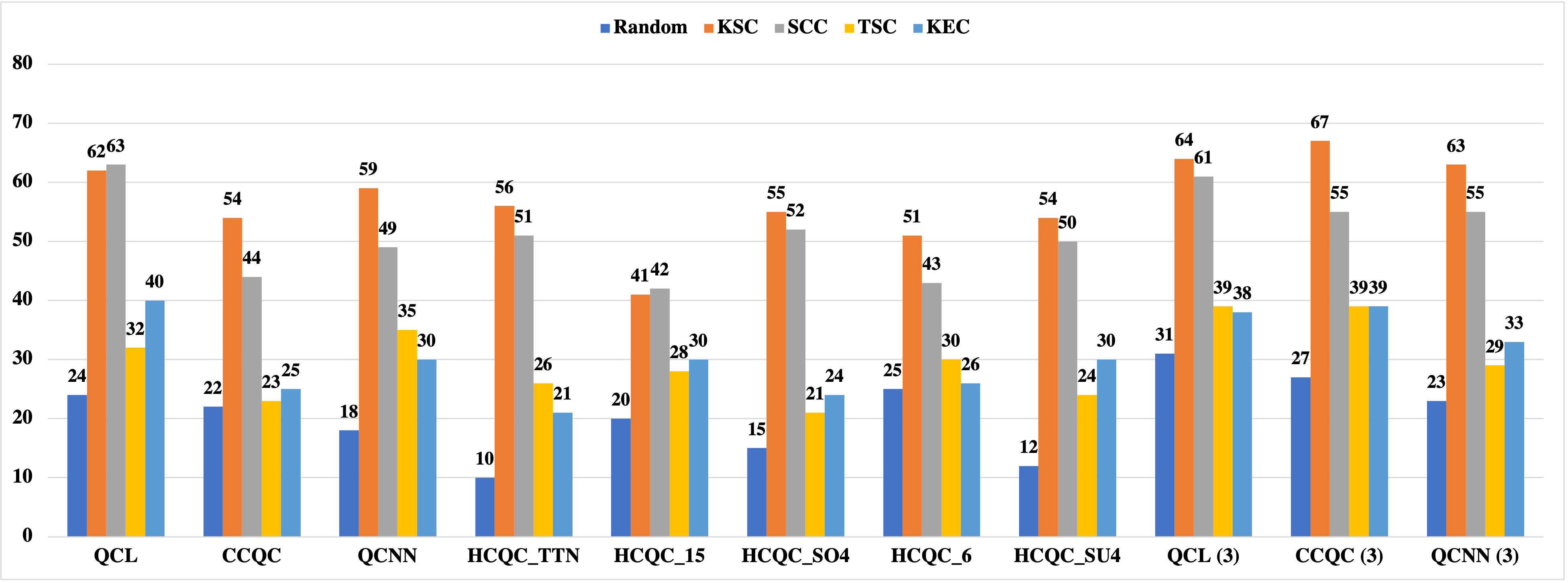
(a) MNIST

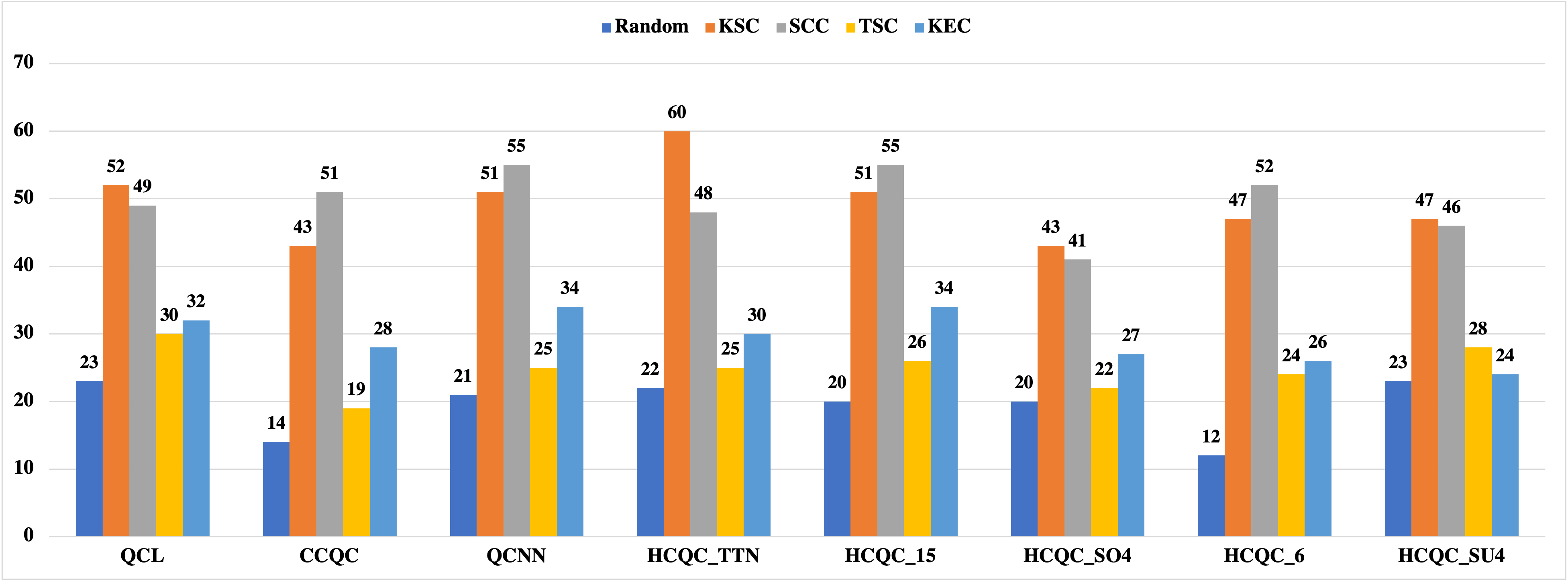
(b) FashionMNIST

Figure 6: Test success rate (TSR) (%) of coverage-guided testing. ”Random” refers to random testing. The x-axis is the testing guidance, and the y-axis is TSR.

In general, KSC and SCC show higher TSRs than TSC and KEC. For example, on MNIST with QCL, KSC achieves a TSR of 62%, while TSC achieves 32%. The reasons are:

(1) KSC involves major-region cells of all basis states, making improving coverage easier by covering just one new cell. It is also relatively simple to increase SCC by covering a new upper or lower region of some state.

(2) TSC measures possible combinations of $k$ basis states, which creates a vast search space, but as discussed in RQ2 (Section 4.2.2), top-$k$ states are relatively stable in QNNs, making it harder for mutants to increase TSC and more likely to be discarded.

(3) KEC’s granularity is limited by the hyperparameter $k$ (i.e., 500), and cells near the ECRatio boundaries (i.e., -50% and 50%) are difficult to cover while preserving image semantics in practice, restricting KEC improvements. In summary, KSC and SCC offer a broader search space for fuzz testing and have less strict requirements for re-enqueuing seeds, leading to higher TSRs.

Answer to RQ3: The experimental results show that QCov effectively guides fuzz testing to generate more defect-inducing cases across diverse datasets and QNNs compared to random testing. Criteria like KSC and SCC generally perform better due to their broader search space.

4.2.4 RQ4: Efficiency

Table 9: Efficiency of QCov (s)

Dataset	Model	Task	KSC	SCC	TKS	KEC
MNIST	QCL	binary	0.14	0.138	0.099	0.219
		ternary	0.138	0.13	0.096	0.223
	CCQC	binary	0.189	0.183	0.146	0.27
		ternary	0.187	0.184	0.147	0.279
	QCNN	binary	0.147	0.142	0.107	0.234
		ternary	0.149	0.143	0.109	0.234
	HCQC_TTN	binary	0.056	0.053	0.017	0.144
	HCQC_15		0.078	0.071	0.034	0.154
	HCQC_SO4		0.086	0.081	0.046	0.168
	HCQC_6		0.107	0.101	0.064	0.185
	HCQC_SU4		0.11	0.104	0.069	0.187
FashionMNIST	QCL	binary	0.134	0.132	0.096	0.228
	CCQC		0.19	0.182	0.146	0.27
	QCNN		0.148	0.143	0.108	0.237
	HCQC_TTN		0.063	0.056	0.017	0.142
	HCQC_15		0.072	0.066	0.033	0.155
	HCQC_SO4		0.088	0.082	0.047	0.17
	HCQC_6		0.103	0.098	0.063	0.188
	HCQC_SU4		0.11	0.104	0.068	0.195

We compute the average time needed by criteria to process a single input, as shown in Table 9. Results show that QCov is efficient overall. KEC takes more time since it requires more information, including MW entanglement and ECRatio. Note that probability-based criteria need to profile training data before evaluation. Considering that this preprocessing phase can be executed only once offline, we ignore the profiling time and only report the time for coverage calculation. Besides, we found that the time costs are more expensive on larger-scale models with more parameters. For example, QCov often needs more time to complete calculations for CCQC than QCL and QCNN. Among the series of HCQC, HCQC_SU4 with 150 parameters consumes the most time.

Answer to RQ4: Although probability-based and entanglement-based criteria involve detailed analysis of individual basis states and qubits, the time costs are not generally expensive.

4.3 Threats to Validity

The selection of datasets and QNN architectures may affect the evaluation. To mitigate this, we used commonly applied datasets, MNIST and FashionMNIST, and four representative QNN architectures with distinct characteristics. Another potential threat is the choice of hyper-parameters in the coverage criteria calculations. We addressed this by evaluating each criterion under multiple configurations, but the effectiveness of QCov still depends on parameters like $k$, which will require further exploration in future work. Randomness in data also affects validity. We repeated each experiment multiple times and reported average results to address this. We plan to scale up experiments in future work. Adversarial test generation also involves randomness, which we mitigated by following recommended settings from prior studies Goodfellow et al. (2014); Kurakin et al. (2016); Papernot et al. (2015); Guo et al. (2018); Shi et al. (2024) and making slight adjustments to balance attack success rates and image quality.

5 Related Work

Quantum Software Testing. Quantum software testing Wang et al. (2018; 2021a); Fortunato et al. (2022a; b); Xia et al. (2024) focuses on verifying the correctness and reliability of quantum programs. Early efforts Wang et al. (2021b); Kumar (2023) have adapted classical coverage criteria to the quantum domain. A recent work Fortunato et al. (2024) proposed Gate Branch Coverage based on quantum controlled gates. However, apart from quantum structural properties, unique coverage criteria focusing on the probabilistic and entangling nature of quantum systems, are still under development to evaluate test adequacy for quantum software. In contrast to existing work, our research focuses on QNNs, which introduce additional complexities due to their special structures. QCov proposes novel coverage criteria to address these challenges, extending beyond traditional quantum program testing by tailoring the criteria to QNN-specific behaviors.

Testing Techniques for DNNs: Test coverage criteria for DNNs have been extensively studied in classical machine learning, with metrics like neuron coverage Pei et al. (2017); Ma et al. (2018a); Liu et al. (2023); Zhou et al. (2021), layer coverage Sun et al. (2018); Ma et al. (2019); Sharma et al. (2021), and path coverage Wang et al. (2019); Xie et al. (2022) assessing input space exploration and network behavior. These metrics identify untested areas in networks, highlighting potential vulnerabilities. In addition, frameworks combining traditional software testing with DNN-specific properties—such as mutation testing Ma et al. (2018b); Humbatova et al. (2021), fuzz testing Guo et al. (2018), concolic testing Sun et al. (2019), metamorphic testing Tian et al. (2017), and combinatorial testing Chandrasekaran et al. (2021)—have proven effective in uncovering DNN defects, particularly when generating adversarial inputs to explore network weaknesses. However, the deterministic nature of DNNs contrasts with the probabilistic behavior of QNNs, requiring new coverage criteria to capture QNN complexities adequately.

Adversarial Robustness of QNNs. Adversarial attacks Goodfellow et al. (2014); Xie et al. (2018); Kurakin et al. (2016); Papernot et al. (2015) are a significant concern in DNNs, where crafted inputs deceive models into incorrect behaviors. Related studies on QNNs are also emerging Lu et al. (2019); Gong & Deng (2022); West et al. (2023); Liu & Wittek (2019). The probabilistic nature of quantum states can make QNNs more resilient to certain attacks Winderl et al. (2023); Guan et al. (2020), but it also introduces new vulnerabilities not found in classical networks Liu & Wittek (2019). QuanTest Shi et al. (2024) proposed the first adversarial testing framework for QNNs which designed a quantum entanglement adequacy (QEA) criterion to guide the adversarial input generation. The difference between our work and QuanTest lies in (1) QuanTest aims to uncover erroneous behaviors in QNNs by generating more adversarial inputs, while QCov focuses on assessing the test adequacy of QNNs and providing guidance for analyzing different model behaviors including major and corner-case ones. Moreover, QCov can detect not only adversarial but also natural-error inputs. (2) The key of the QuanTest method is the QEA, which quantifies the entanglement change for each individual input. QCov refines the original QEA by introducing ECRatio to alleviate the incomparability between inputs and evaluate overall test adequacy, as mentioned in Section 3.2. Beyond entanglement, QCov also utilizes basis state probability to measure the exploration of solution space, presenting a more systematic and comprehensive testing framework.

6 Concluding Remarks

This paper addresses the need for systematic QNN testing by introducing QCov, a set of multi-granularity coverage criteria specifically designed for QNNs. These criteria capture the unique behaviors of QNNs, considering their quantum characteristics such as superposition and entanglement. We evaluated QCov using two datasets, four benchmark QNN architectures, and six adversarial test generation techniques. The results show that QCov can effectively detect subtle changes in QNNs’ behaviors and generate more erroneous inputs by guiding the fuzz testing. These findings highlight QCov’s potential to enhance the robustness and reliability of QNNs, making it a valuable tool for QNN testing. In the future, we plan to evaluate QCov in a broader range of datasets and QNN architectures, focusing on kernel-based QNNs and Quantum Recurrent Neural Networks (QRNNs). We will also investigate the decomposition of quantum circuits to enable more fine-grained testing for QNNs to explore their robustness further.

References

- Alam et al. (2021) Maha Anis Alam, Satwik Kundu, Rasit Onur Topaloglu, and Swaroop Ghosh. Quantum-classical hybrid machine learning for image classification (iccad special session paper). 2021 IEEE/ACM International Conference On Computer Aided Design (ICCAD), pp. 1–7, 2021.
- Banchi & Crooks (2020) Leonardo Banchi and Gavin E. Crooks. Measuring analytic gradients of general quantum evolution with the stochastic parameter shift rule. Quantum, 5:386, 2020.
- Bausch (2020) Johannes Bausch. Recurrent quantum neural networks. ArXiv, abs/2006.14619, 2020.
- Benedetti et al. (2019) Marcello Benedetti, Erika Lloyd, Stefan H. Sack, and Mattia Fiorentini. Parameterized quantum circuits as machine learning models. Quantum Science and Technology, 4, 2019.
- Bergholm et al. (2018) Ville Bergholm, Josh A. Izaac, Maria Schuld, Christian Gogolin, Ankit Khandelwal, and Nathan Killoran. Pennylane: Automatic differentiation of hybrid quantum-classical computations. ArXiv, abs/1811.04968, 2018.
- Chandrasekaran et al. (2021) Jaganmohan Chandrasekaran, Yu Lei, Raghu N. Kacker, and D. Richard Kuhn. A combinatorial approach to testing deep neural network-based autonomous driving systems. 2021 IEEE International Conference on Software Testing, Verification and Validation Workshops (ICSTW), pp. 57–66, 2021.
- Chu et al. (2023a) Cheng Chu, Fan Chen, Philip Richerme, and Lei Jiang. Qdoor: Exploiting approximate synthesis for backdoor attacks in quantum neural networks. 2023 IEEE International Conference on Quantum Computing and Engineering (QCE), 01:1098–1106, 2023a.
- Chu et al. (2023b) Cheng Chu, Lei Jiang, Martin Swany, and Fan Chen. Qtrojan: A circuit backdoor against quantum neural networks. ICASSP 2023 - 2023 IEEE International Conference on Acoustics, Speech and Signal Processing (ICASSP), pp. 1–5, 2023b.
- Cong & Duan (2015) Iris Cong and Luming Duan. Quantum discriminant analysis for dimensionality reduction and classification. New Journal of Physics, 18, 2015.
- Cong et al. (2018) Iris Cong, Soonwon Choi, and Mikhail D. Lukin. Quantum convolutional neural networks. Nature Physics, 15:1273 – 1278, 2018.
- Dang et al. (2018) Yijie Dang, Nan Jiang, Hao Hu, Zhuoxiao Ji, and Wenyin Zhang. Image classification based on quantum k-nearest-neighbor algorithm. Quantum Information Processing, 17, 2018.
- Fan et al. (2023) Fan Fan, Yilei Shi, Tobias Guggemos, and Xiaoxiang Zhu. Hybrid quantum-classical convolutional neural network model for image classification. IEEE transactions on neural networks and learning systems, PP, 2023.
- Fortunato et al. (2022a) Daniel Fortunato, José Campos, and Rui Abreu. Mutation testing of quantum programs written in qiskit. 2022 IEEE/ACM 44th International Conference on Software Engineering: Companion Proceedings (ICSE-Companion), pp. 358–359, 2022a.
- Fortunato et al. (2022b) Daniel Fortunato, José Campos, and Rui Abreu. Qmutpy: a mutation testing tool for quantum algorithms and applications in qiskit. Proceedings of the 31st ACM SIGSOFT International Symposium on Software Testing and Analysis, 2022b.
- Fortunato et al. (2024) Daniel Fortunato, José Campos, and Rui Abreu. Gate branch coverage: A metric for quantum software testing. Proceedings of the 1st ACM International Workshop on Quantum Software Engineering: The Next Evolution, 2024.
- Gao et al. (2018) Xun Gao, Z.-Y. Zhang, Z.-Y. Zhang, Luming Duan, and Luming Duan. A quantum machine learning algorithm based on generative models. Science Advances, 4, 2018.
- Gong & Deng (2022) Weiyuan Gong and Dong-Ling Deng. Universal adversarial examples and perturbations for quantum classifiers. National Science Review, 9(6):nwab130, 2022.
- Goodfellow et al. (2014) Ian J. Goodfellow, Jonathon Shlens, and Christian Szegedy. Explaining and harnessing adversarial examples. CoRR, abs/1412.6572, 2014.
- Guan et al. (2020) Ji Guan, Wang Fang, and Mingsheng Ying. Robustness verification of quantum classifiers. In International Conference on Computer Aided Verification, 2020.
- Guo et al. (2018) Jianmin Guo, Yu Jiang, Yue Zhao, Quan Chen, and Jiaguang Sun. Dlfuzz: differential fuzzing testing of deep learning systems. Proceedings of the 2018 26th ACM Joint Meeting on European Software Engineering Conference and Symposium on the Foundations of Software Engineering, 2018.
- He et al. (2015) Kaiming He, X. Zhang, Shaoqing Ren, and Jian Sun. Deep residual learning for image recognition. 2016 IEEE Conference on Computer Vision and Pattern Recognition (CVPR), pp. 770–778, 2015.
- Henderson et al. (2019) Maxwell P. Henderson, Samriddhi Shakya, Shashindra Pradhan, and Tristan Cook. Quanvolutional neural networks: powering image recognition with quantum circuits. Quantum Machine Intelligence, 2, 2019.
- Howard et al. (2017) Andrew G. Howard, Menglong Zhu, Bo Chen, Dmitry Kalenichenko, Weijun Wang, Tobias Weyand, Marco Andreetto, and Hartwig Adam. Mobilenets: Efficient convolutional neural networks for mobile vision applications. ArXiv, abs/1704.04861, 2017.
- Humbatova et al. (2021) Nargiz Humbatova, Gunel Jahangirova, and Paolo Tonella. Deepcrime: mutation testing of deep learning systems based on real faults. Proceedings of the 30th ACM SIGSOFT International Symposium on Software Testing and Analysis, 2021.
- Hur et al. (2021) Tak Hur, Lee Yeong Kim, and Daniel Kyungdeock Park. Quantum convolutional neural network for classical data classification. Quantum Machine Intelligence, 4, 2021.
- Kumar (2023) Ajay Kumar. Formalization of structural test cases coverage criteria for quantum software testing. International Journal of Theoretical Physics, 62, 2023.
- Kurakin et al. (2016) Alexey Kurakin, Ian J. Goodfellow, and Samy Bengio. Adversarial examples in the physical world. ArXiv, abs/1607.02533, 2016.
- LeCun et al. (1998a) Yann LeCun, Léon Bottou, Yoshua Bengio, and Patrick Haffner. Gradient-based learning applied to document recognition. Proc. IEEE, 86:2278–2324, 1998a.
- LeCun et al. (1998b) Yann LeCun, Léon Bottou, Yoshua Bengio, and Patrick Haffner. Gradient-based learning applied to document recognition. Proc. IEEE, 86:2278–2324, 1998b.
- Li et al. (2022a) Wei Li, Peng-Cheng Chu, Guangchao Liu, Yanbing Tian, Tian-Hui Qiu, and Shumei Wang. An image classification algorithm based on hybrid quantum classical convolutional neural network. Quantum Eng., 2022:1–9, 2022a.
- Li et al. (2022b) Weikang Li, Zhide Lu, and Dong-Ling Deng. Quantum neural network classifiers: A tutorial. ArXiv, abs/2206.02806, 2022b.
- Liu & Wittek (2019) Nana Liu and Peter Wittek. Vulnerability of quantum classification to adversarial perturbations. Physical Review A, 2019.
- Liu et al. (2023) Y. Liu, Chris Xing Tian, Haoliang Li, Lei Ma, and Shiqi Wang. Neuron activation coverage: Rethinking out-of-distribution detection and generalization. ArXiv, abs/2306.02879, 2023.
- Lu et al. (2019) Sirui Lu, Luming Duan, and Dong-Ling Deng. Quantum adversarial machine learning. ArXiv, abs/2001.00030, 2019.
- Ma et al. (2018a) L. Ma, Felix Juefei-Xu, Fuyuan Zhang, Jiyuan Sun, Minhui Xue, Bo Li, Chunyang Chen, Ting Su, Li Li, Yang Liu, Jianjun Zhao, and Yadong Wang. Deepgauge: Multi-granularity testing criteria for deep learning systems. 2018 33rd IEEE/ACM International Conference on Automated Software Engineering (ASE), pp. 120–131, 2018a.
- Ma et al. (2018b) L. Ma, Fuyuan Zhang, Jiyuan Sun, Minhui Xue, Bo Li, Felix Juefei-Xu, Chao Xie, Li Li, Yang Liu, Jianjun Zhao, and Yadong Wang. Deepmutation: Mutation testing of deep learning systems. 2018 IEEE 29th International Symposium on Software Reliability Engineering (ISSRE), pp. 100–111, 2018b.
- Ma et al. (2019) L. Ma, Felix Juefei-Xu, Minhui Xue, Bo Li, Li Li, Yang Liu, and Jianjun Zhao. Deepct: Tomographic combinatorial testing for deep learning systems. 2019 IEEE 26th International Conference on Software Analysis, Evolution and Reengineering (SANER), pp. 614–618, 2019.
- Maier et al. (2004) Thomas Maier, Mark Jarrell, and Matthias H. Hettler. Quantum cluster theories. Reviews of Modern Physics, 77:1027–1080, 2004.
- Meyer & Wallach (2001) David A. Meyer and Nolan Wallach. Global entanglement in multiparticle systems. Journal of Mathematical Physics, 43:4273–4278, 2001.
- Mitarai et al. (2018) Kosuke Mitarai, Makoto Negoro, Masahiro Kitagawa, and Keisuke Fujii. Quantum circuit learning. Physical Review A, 2018.
- Nair & Hinton (2010) Vinod Nair and Geoffrey E. Hinton. Rectified linear units improve restricted boltzmann machines. In International Conference on Machine Learning, 2010.
- Papernot et al. (2015) Nicolas Papernot, Patrick Mcdaniel, Somesh Jha, Matt Fredrikson, Z. Berkay Celik, and Ananthram Swami. The limitations of deep learning in adversarial settings. 2016 IEEE European Symposium on Security and Privacy (EuroS&P), pp. 372–387, 2015.
- Paszke et al. (2019) Adam Paszke, Sam Gross, Francisco Massa, Adam Lerer, James Bradbury, Gregory Chanan, Trevor Killeen, Zeming Lin, Natalia Gimelshein, Luca Antiga, Alban Desmaison, Andreas Köpf, Edward Yang, Zach DeVito, Martin Raison, Alykhan Tejani, Sasank Chilamkurthy, Benoit Steiner, Lu Fang, Junjie Bai, and Soumith Chintala. Pytorch: An imperative style, high-performance deep learning library. ArXiv, abs/1912.01703, 2019.
- Pei et al. (2017) Kexin Pei, Yinzhi Cao, Junfeng Yang, and Suman Sekhar Jana. Deepxplore: Automated whitebox testing of deep learning systems. Proceedings of the 26th Symposium on Operating Systems Principles, 2017.
- Peters et al. (2021) Evan Peters, João Caldeira, Alan K. Ho, Stefan Leichenauer, Masoud Mohseni, Hartmut Neven, Panagiotis Spentzouris, Doug Strain, and Gabriel N. Perdue. Machine learning of high dimensional data on a noisy quantum processor. npj Quantum Information, 7, 2021.
- Rebentrost et al. (2013) Patrick Rebentrost, Masoud Mohseni, and Seth Lloyd. Quantum support vector machine for big feature and big data classification. Physical review letters, 113 13:130503, 2013.
- Schuld & Petruccione (2018) Maria Schuld and Francesco Petruccione. Quantum machine learning. 2018.
- Schuld et al. (2018) Maria Schuld, Alex Bocharov, Krysta Marie Svore, and Nathan Wiebe. Circuit-centric quantum classifiers. Physical Review A, 2018.
- Sharma et al. (2021) Alok Sharma, Artem Lysenko, Keith A. Boroevich, Edwin Vans, and Tatsuhiko Tsunoda. Deepfeature: feature selection in nonimage data using convolutional neural network. Briefings in Bioinformatics, 22, 2021.
- Shi et al. (2022) Jinjing Shi, Wenxuan Wang, Xiaoping Lou, Shenmin Zhang, and Xuelong Li. Parameterized hamiltonian learning with quantum circuit. IEEE Transactions on Pattern Analysis and Machine Intelligence, 45:6086–6095, 2022.
- Shi et al. (2024) Jinjing Shi, Zimeng Xiao, Heyuan Shi, Yu Jiang, and Xuelong Li. Quantest: Entanglement-guided testing of quantum neural network systems. ArXiv, abs/2402.12950, 2024.
- Shi et al. (2023) Mingrui Shi, Haozhen Situ, and Cai Zhang. Hybrid quantum neural network structures for image multi-classification. Physica Scripta, 99, 2023.
- Sun et al. (2018) Youcheng Sun, Xiaowei Huang, and Daniel Kroening. Testing deep neural networks. ArXiv, abs/1803.04792, 2018.
- Sun et al. (2019) Youcheng Sun, Xiaowei Huang, Daniel Kroening, James Sharp, Matthew Hill, and Rob Ashmore. Deepconcolic: Testing and debugging deep neural networks. 2019 IEEE/ACM 41st International Conference on Software Engineering: Companion Proceedings (ICSE-Companion), pp. 111–114, 2019.
- Tian et al. (2017) Yuchi Tian, Kexin Pei, Suman Sekhar Jana, and Baishakhi Ray. Deeptest: Automated testing of deep-neural-network-driven autonomous cars. 2018 IEEE/ACM 40th International Conference on Software Engineering (ICSE), pp. 303–314, 2017.
- Wang et al. (2019) Dong Wang, Ziyuan Wang, Chunrong Fang, Yanshan Chen, and Zhenyu Chen. Deeppath: Path-driven testing criteria for deep neural networks. 2019 IEEE International Conference On Artificial Intelligence Testing (AITest), pp. 119–120, 2019.
- Wang et al. (2018) Jiyuan Wang, Ming Gao, Yu Jiang, Jian-Guang Lou, Yue Gao, D. Zhang, and Jiaguang Sun. Quanfuzz: Fuzz testing of quantum program. ArXiv, abs/1810.10310, 2018.
- Wang et al. (2021a) Jiyuan Wang, Qian Zhang, Guoqing Harry Xu, and Miryung Kim. Qdiff: Differential testing of quantum software stacks. 2021 36th IEEE/ACM International Conference on Automated Software Engineering (ASE), pp. 692–704, 2021a.
- Wang et al. (2021b) Xinyi Wang, Paolo Arcaini, Tao Yue, and Sajid Ali. Quito: a coverage-guided test generator for quantum programs. 2021 36th IEEE/ACM International Conference on Automated Software Engineering (ASE), pp. 1237–1241, 2021b.
- Wang et al. (2024) Zhiyu Wang, Sihan Xu, Lingling Fan, Xiangrui Cai, Linyu Li, and Zheli Liu. Can coverage criteria guide failure discovery for image classifiers? an empirical study. ACM Transactions on Software Engineering and Methodology, 2024.
- West et al. (2023) Maxwell T. West, Shu Lok Tsang, Jia Shun Low, Charles D. Hill, Christopher Leckie, Lloyd C. L. Hollenberg, Sarah Monazam Erfani, and Muhammad Usman. Towards quantum enhanced adversarial robustness in machine learning. Nature Machine Intelligence, 5:581 – 589, 2023.
- Wiebe et al. (2012) Nathan Wiebe, Daniel Braun, and Seth Lloyd. Quantum algorithm for data fitting. Physical review letters, 109(5):050505, 2012.
- Winderl et al. (2023) David Winderl, Nicola Franco, and Jeanette Miriam Lorenz. Quantum neural networks under depolarization noise: Exploring white-box attacks and defenses. ArXiv, abs/2311.17458, 2023.
- Xia et al. (2024) Shangzhou Xia, Jianjun Zhao, Fuyuan Zhang, and Xiaoyu Guo. Concolic testing of quantum programs. ArXiv, abs/2405.04860, 2024.
- Xiao et al. (2017) Han Xiao, Kashif Rasul, and Roland Vollgraf. Fashion-mnist: a novel image dataset for benchmarking machine learning algorithms. ArXiv, abs/1708.07747, 2017.
- Xie et al. (2018) Cihang Xie, Zhishuai Zhang, Jianyu Wang, Yuyin Zhou, Zhou Ren, and Alan Loddon Yuille. Improving transferability of adversarial examples with input diversity. 2019 IEEE/CVF Conference on Computer Vision and Pattern Recognition (CVPR), pp. 2725–2734, 2018.
- Xie et al. (2019) Xiaofei Xie, L. Ma, Felix Juefei-Xu, Minhui Xue, Hongxu Chen, Yang Liu, Jianjun Zhao, Bo Li, Jianxiong Yin, and S. See. Deephunter: a coverage-guided fuzz testing framework for deep neural networks. Proceedings of the 28th ACM SIGSOFT International Symposium on Software Testing and Analysis, 2019.
- Xie et al. (2022) Xiaofei Xie, Tianlin Li, Jian Wang, L. Ma, Qing Guo, Felix Juefei-Xu, and Yang Liu. Npc: Neuron path coverage via characterizing decision logic of deep neural networks. ACM Transactions on Software Engineering and Methodology (TOSEM), 31:1 – 27, 2022.
- Xie et al. (2024) Xuan Xie, Jiayang Song, Yuheng Huang, Da Song, Fuyuan Zhang, Felix Juefei-Xu, and Lei Ma. Lecov: Multi-level testing criteria for large language models. 2024.
- Yu et al. (2024) Wenbin Yu, Lei Yin, Chengjun Zhang, Yadang Chen, and Alex X. Liu. Application of quantum recurrent neural network in low-resource language text classification. IEEE Transactions on Quantum Engineering, 5:1–13, 2024.
- Zhang et al. (2020) Jie M Zhang, Mark Harman, Lei Ma, and Yang Liu. Machine learning testing: Survey, landscapes and horizons. IEEE Transactions on Software Engineering, 48(1):1–36, 2020.
- Zhou et al. (2021) Zhiyang Zhou, Wensheng Dou, Jie Liu, Chenxin Zhang, Jun Wei, and Dan Ye. Deepcon: Contribution coverage testing for deep learning systems. 2021 IEEE International Conference on Software Analysis, Evolution and Reengineering (SANER), pp. 189–200, 2021.